CSE 676 · Module 11 · Week 8
Structured Distributions
Directed graphical models, factorization, conditional independence and d-separation, explaining away, naive Bayes, Markov blankets, and sequence models with hidden variables.
Companion reading: Bishop & Bishop, Deep Learning: Foundations and Concepts, chapter 11, “Structured Distributions”
By the end of this module you can
- Write down the joint distribution that a directed acyclic graph encodes, find a topological order, and count the parameters of full tables, chains, tied chains, and fully factorized models.
- Replace a conditional probability table by a logistic or neural conditional, and explain when the smaller model predicts better on held-out data.
- Derive the mean and covariance of a linear-Gaussian network by recursion, check them against the matrix formula and ancestral samples, and read the Markov blankets off its precision matrix.
- Draw a model with plates, deterministic parameters, latent and observed nodes, and turn the drawing into a log joint that code can evaluate.
- Verify the tail-to-tail, head-to-tail, and head-to-head rules numerically, explain explaining away with your own numbers, and implement d-separation and test it against brute-force independence checks.
- Derive the Markov blanket of a node, show numerically that it screens the node off from the rest of the graph, and describe the two “filters” a graph defines.
- Compare Markov chains of increasing order on real text, explain why their parameter counts explode, and show that a state-space model’s observations are not Markov at any order.
- Explain how neural networks parametrize the conditionals of a graph in the models of later modules, from autoregressive language models to VAEs and diffusion models.
Contents
A neural network classifier, as we built it in module 05 and module 06, defines a single conditional distribution, \(p(t \mid \mathbf{x}, \mathbf{w}) = y^{t}(1 - y)^{1 - t}\) with \(y = y(\mathbf{x}, \mathbf{w})\). The network may have millions of weights, but the distribution itself has a simple shape: one Bernoulli variable, given the input. Many of the models in the second half of this course are richer than that. A language model defines a distribution over whole sequences of tokens; a variational autoencoder has an unobserved code that generates an image; a diffusion model chains together many progressively noisier versions of an image. To describe such models we need a language for structured distributions: joint distributions over many variables that are built from small conditional pieces.
That language is the probabilistic graphical model. A graph shows at a glance which variables depend directly on which, it tells us which independence properties hold without any algebra, and it tells us how to sample from the model and how to write its log-likelihood, which is the loss we train with. Neural networks enter as the functions that parametrize the conditional pieces. This module develops the directed version of the language, the one used throughout deep learning.
Much of the material also appears in Intro to ML, module 08, which goes further: undirected graphs, factor graphs, and exact inference by message passing. Here we give a compact, self-contained account, check every claim with NumPy, and point out where each idea is used by the deep generative models of modules 12–20.
import os
import urllib.request
from itertools import combinations, product
import numpy as np
from scipy.special import expit, logsumexp

np.set_printoptions(precision=4, suppress=True)
rng = np.random.default_rng(11)
Graphical models
Everything we do with probabilities comes down to the sum rule and the product rule of module 02. A graph adds no new mathematics. What it adds is a picture of how a model is put together, which helps us design new models, read off their properties, and organize the computations of inference and learning.
Directed graphs
A graph consists of nodes (also called vertices) joined by links (also called edges). In a probabilistic graphical model every node stands for a random variable, or a group of variables, and the links say which variables are directly coupled. When every link carries an arrow we have a directed graphical model, also called a Bayesian network. Arrows are natural for describing how data are generated: a cause points to its effect, a latent code points to the image it produces.
There is also an undirected family, Markov random fields, whose links carry no arrows and express soft constraints between variables, such as neighboring pixels that tend to agree. Directed and undirected graphs are both special cases of factor graphs. We stay with directed graphs; the undirected ones are covered in Intro to ML, module 08.
Watch out. A neural network diagram and a graphical model look alike, with circles and arrows in both, but they mean different things. In a network diagram a node is a deterministic value computed from its inputs. In a graphical model a node is a random variable, and an arrow means “the distribution of this variable depends on that one”. The graph neural networks of module 13 operate on graphs whose nodes hold deterministic vectors, which is a third meaning again.
Factorization
Take any joint distribution \(p(a, b, c)\). Two applications of the product rule give
\[p(a, b, c) = p(c \mid a, b)\, p(a, b) = p(c \mid a, b)\, p(b \mid a)\, p(a).\]To draw this as a graph, make one node per variable, and for each factor draw an arrow into the variable on the left of the bar from each variable on the right. So \(a\) gets no incoming arrows, \(b\) gets one from \(a\), and \(c\) gets arrows from \(a\) and \(b\). If there is an arrow from \(a\) to \(b\), then \(a\) is a parent of \(b\) and \(b\) is a child of \(a\). The same trick works for \(K\) variables in any order:
\[p(x_1, \dots, x_K) = p(x_K \mid x_1, \dots, x_{K-1}) \cdots p(x_2 \mid x_1)\, p(x_1).\]Every node now receives an arrow from every node before it, so the graph is fully connected. This factorization holds for every distribution, which also means it says nothing about any particular one. Notice that the left side is symmetric in the variables while the right side is not: a different ordering would give a different, equally valid, graph.
The interesting information in a graph is carried by the missing arrows. Given any directed graph, we define the joint distribution as the product of one conditional per node, each conditioned only on that node’s parents:
Result. The joint distribution of a directed graphical model over \(x_1, \dots, x_K\) is
\[p(x_1, \dots, x_K) = \prod_{k=1}^{K} p(x_k \mid \mathrm{pa}(k)),\]where \(\mathrm{pa}(k)\) is the set of parents of node \(k\). If each conditional is normalized, so is the product.
To see the normalization, sum over the variables one at a time, starting with a node that has no children. That node appears in only one factor, its own conditional, and summing it out gives 1. Removing it leaves a smaller graph of the same kind, so we repeat until nothing is left. The argument needs a node without children at every step, and that is guaranteed by the one restriction we place on the graph: it must have no directed cycles, meaning no route that follows the arrows and returns to its start. Such a graph is a directed acyclic graph (DAG). Being acyclic is the same as having a topological order, a numbering of the nodes in which every arrow goes from a lower to a higher number. We use the same symbol for a node and its variable. Nodes can hold scalars, vectors, or whole images; nothing in the factorization changes.
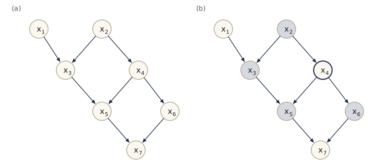
Our running example is the graph in the figure. We store a graph as a dictionary from each node to the tuple of its parents; the dictionary order is deliberately scrambled. Kahn’s algorithm finds a topological order by repeatedly emitting the nodes whose parents have all been emitted, and it reports a cycle if it gets stuck.
parents = {                      # node: its parents (the listing order is not topological)
    "x7": ("x5", "x6"),
    "x3": ("x1", "x2"),
    "x5": ("x3", "x4"),
    "x1": (),
    "x6": ("x4",),
    "x2": (),
    "x4": ("x2",),
}

def topological_order(parents):
    """Kahn's algorithm: emit every node whose parents have all been emitted; repeat."""
    order, done, remaining = [], set(), dict(parents)
    while remaining:
        ready = sorted(v for v, pa in remaining.items() if set(pa) <= done)
        if not ready:
            raise ValueError("directed cycle among " + ", ".join(sorted(remaining)))
        for v in ready:
            order.append(v)
            done.add(v)
            del remaining[v]
    return order

def factor_string(parents, order):
    return " ".join("p({}{})".format(v, " | " + ",".join(parents[v]) if parents[v] else "")
                    for v in order)

order = topological_order(parents)
print("topological order:", order)
print("p(x) =", factor_string(parents, order))
topological order: ['x1', 'x2', 'x3', 'x4', 'x5', 'x6', 'x7']
p(x) = p(x1) p(x2) p(x3 | x1,x2) p(x4 | x2) p(x5 | x3,x4) p(x6 | x4) p(x7 | x5,x6)
A graph with a cycle has no topological order and does not define a distribution this way:
topological_order({"a": ("c",), "b": ("a",), "c": ("b",)})
ValueError: directed cycle among a, b, c
Discrete variables
Suppose every variable is discrete. The conditional \(p(x_k \mid \mathrm{pa}(k))\) is then a conditional probability table (CPT): for each setting of the parents, a probability vector over the states of \(x_k\). We store it as an array with one axis per parent and a last axis for \(x_k\). Multiplying all the CPTs together, with each axis lined up with its variable, gives the joint table. np.einsum does exactly that product.
def random_cpts(parents, states, rng):
    """A random CPT per node, shape (states of each parent..., states of the node)."""
    return {v: rng.dirichlet(np.ones(states[v]), size=tuple(states[u] for u in pa))
            for v, pa in parents.items()}

def joint_table(parents, cpts, order):
    """p(x) = prod_k p(x_k | pa(k)) as a dense array with one axis per variable, in `order`."""
    axis = {v: i for i, v in enumerate(order)}
    args = []
    for v in order:
        args += [cpts[v], [axis[u] for u in parents[v]] + [axis[v]]]
    return np.einsum(*args, list(range(len(order))))

states = {v: 2 for v in parents}                 # all seven variables binary
cpts = random_cpts(parents, states, rng)
P = joint_table(parents, cpts, order)
print("joint table shape", P.shape, "  sum", f"{P.sum():.12f}")
print("p(x3 = 1 | x1, x2) from the CPT:\n", cpts["x3"][..., 1])
joint table shape (2, 2, 2, 2, 2, 2, 2)   sum 1.000000000000
p(x3 = 1 | x1, x2) from the CPT:
 [[0.7068 0.7019]
 [0.1131 0.4796]]
With binary variables the joint table has \(2^7 = 128\) entries, and the graph lets us specify it with far fewer numbers. Let us count them in general. A single variable with \(K\) states needs \(K - 1\) numbers, since its probabilities sum to one. A full joint table over \(M\) such variables needs \(K^M - 1\), which grows exponentially. A node with \(m\) parents, each with \(K\) states, needs \(K - 1\) numbers for each of the \(K^m\) parent settings, so a graph needs \(\sum_k (K - 1) K^{\lvert \mathrm{pa}(k) \rvert}\) numbers in total. Three graphs mark the range:
- Fully connected: node \(k\) has \(k - 1\) parents, and the counts add up to \(K^M - 1\). Any distribution can be represented.
- No links: \(M(K - 1)\) numbers, linear in \(M\), but the variables are forced to be independent.
- A chain \(x_1 \to x_2 \to \cdots \to x_M\): \(K - 1 + (M - 1)K(K - 1)\), still linear in \(M\), yet every variable can depend on every other through the chain.
A second way to save parameters is parameter sharing, also called tying: let all the conditionals \(p(x_i \mid x_{i-1})\) of the chain use one and the same table. The count drops to \(K - 1 + K(K - 1) = K^2 - 1\), independent of the length. Tying is everywhere in deep learning: a convolutional layer uses the same kernel at every position (module 10), and a language model uses the same network to predict every token.
def n_params(parents, K):
    """Free numbers in the CPTs when every variable has K states."""
    return sum((K - 1) * K ** len(pa) for pa in parents.values())

M, K = 10, 4
names = [f"v{i}" for i in range(1, M + 1)]
graphs = {
    "fully connected": {v: tuple(names[:i]) for i, v in enumerate(names)},
    "chain": {v: tuple(names[max(i - 1, 0):i]) for i, v in enumerate(names)},
    "no links": {v: () for v in names},
}
print(f"M = {M} variables with K = {K} states")
for name, pa in graphs.items():
    print(f"  {name:16s} {n_params(pa, K):>9,d}")
print(f"  {'tied chain':16s} {K - 1 + K * (K - 1):>9,d}")
print(f"  full joint table {K ** M - 1:>9,d}")
print(f"running example, binary: {n_params(parents, 2)} numbers instead of {2 ** 7 - 1}")
M = 10 variables with K = 4 states
  fully connected  1,048,575
  chain                  111
  no links                30
  tied chain              15
  full joint table 1,048,575
running example, binary: 18 numbers instead of 127
Conditionals as functions
Tables have a second problem besides their size. Consider a binary node \(y\) with \(M\) binary parents \(x_1, \dots, x_M\). Its CPT has \(2^M\) entries, one probability for each parent setting, and each entry is learned only from the training examples with exactly that setting. With \(M = 10\) there are 1024 settings, and a data set of a few hundred examples leaves most of them unseen.
The remedy is to make the conditional a function of the parents with a few parameters. The simplest choice is the logistic model of module 05:
\[p(y = 1 \mid x_1, \dots, x_M) = \sigma\Bigl(w_0 + \sum_{i=1}^{M} w_i x_i\Bigr) = \sigma(\mathbf{w}^{\mathrm{T}}\mathbf{x}),\]where \(\mathbf{x} = (1, x_1, \dots, x_M)^{\mathrm{T}}\) includes a constant for the bias. It has \(M + 1\) parameters, linear in \(M\) rather than exponential, at the price of a restricted family: the log-odds must be a sum of separate effects. Replacing \(\mathbf{w}^{\mathrm{T}}\mathbf{x}\) by a neural network \(a(\mathbf{x}, \mathbf{w})\) gives a family that can represent any table as the network grows, while a small network still has few parameters. This is the step that connects graphical models to deep learning: every conditional in a graph can be a neural network that takes the parents as input and outputs the parameters of a distribution over the child.
Let us test the three options. The true conditional has an interaction between \(x_1\) and \(x_2\) (each raises the log-odds alone, but together they roughly cancel), which the logistic model cannot express. We fit a table (with one pseudo-count per outcome, so unseen settings get probability 1/2), a logistic model, and a one-hidden-layer network with 8 tanh units. The logistic model and the network get a Gaussian prior of precision 3 on their weights, which acts as weight decay. We measure the average negative log-likelihood on 20,000 test examples.
M = 10
mu_x = rng.uniform(0.3, 0.7, size=M)                     # p(x_i = 1) for the parent nodes

def a_true(X):                                            # true log-odds of y given the parents
    return (-1.5 + 1.2 * X[:, 0] + 1.2 * X[:, 1] - 2.8 * X[:, 0] * X[:, 1]
            + 0.8 * X[:, 2] + 0.6 * X[:, 3] - 0.7 * X[:, 4])

def sample_xy(n, rng):
    X = (rng.random((n, M)) < mu_x).astype(float)
    y = (rng.random(n) < expit(a_true(X))).astype(float)
    return X, y

def nll(p, y):
    p = np.clip(p, 1e-12, 1 - 1e-12)
    return -np.mean(y * np.log(p) + (1 - y) * np.log(1 - p))

def fit_table(X, y):                                      # 2^M probabilities, one per setting
    idx = (X @ 2 ** np.arange(M)).astype(int)
    n1 = np.bincount(idx, weights=y, minlength=2 ** M)
    n = np.bincount(idx, minlength=2 ** M)
    return lambda Xq: ((n1 + 1) / (n + 2))[(Xq @ 2 ** np.arange(M)).astype(int)]

def fit_logistic(X, y, alpha=3.0, iters=25):         # Newton (IRLS), prior N(0, I / alpha)
    Phi = np.hstack([np.ones((len(X), 1)), X])
    w = np.zeros(M + 1)
    for _ in range(iters):
        p = expit(Phi @ w)
        g = Phi.T @ (p - y) + alpha * w
        H = (Phi * (p * (1 - p))[:, None]).T @ Phi + alpha * np.eye(M + 1)
        w -= np.linalg.solve(H, g)
    return lambda Xq: expit(w[0] + Xq @ w[1:])

def fit_mlp(X, y, H=8, alpha=3.0, steps=1500, lr=0.03, seed=0):
    """y = sigma(w2^T tanh(W1^T x + b1) + b2), trained full-batch with Adam."""
    r = np.random.default_rng(seed)
    params = [r.normal(0, M ** -0.5, (M, H)), np.zeros(H), r.normal(0, H ** -0.5, H), np.zeros(1)]
    m1 = [np.zeros_like(q) for q in params]
    m2 = [np.zeros_like(q) for q in params]
    lam = alpha / len(X)                                   # the prior, per example
    for t in range(1, steps + 1):
        W1, b1, w2, b2 = params
        Z = np.tanh(X @ W1 + b1)
        da = (expit(Z @ w2 + b2) - y) / len(X)             # dE/da for the mean cross-entropy
        dZ = np.outer(da, w2) * (1 - Z ** 2)
        grads = [X.T @ dZ + lam * W1, dZ.sum(0), Z.T @ da + lam * w2, da.sum(keepdims=True)]
        for i, g in enumerate(grads):
            m1[i] = 0.9 * m1[i] + 0.1 * g
            m2[i] = 0.999 * m2[i] + 0.001 * g * g
            params[i] = params[i] - lr * (m1[i] / (1 - 0.9 ** t)) / (
                np.sqrt(m2[i] / (1 - 0.999 ** t)) + 1e-8)
    W1, b1, w2, b2 = params
    return lambda Xq: expit(np.tanh(Xq @ W1 + b1) @ w2 + b2)

X_test, y_test = sample_xy(20000, rng)
print(f"true conditional: test NLL {nll(expit(a_true(X_test)), y_test):.4f}")
print(f"parameters: table {2 ** M}, logistic {M + 1}, network {M * 8 + 8 + 8 + 1}")
print("    N    table  logistic  network")
for N in [100, 1000, 5000]:
    X, y = sample_xy(N, np.random.default_rng(N))
    scores = [nll(fit(X, y)(X_test), y_test) for fit in (fit_table, fit_logistic, fit_mlp)]
    print(f"{N:5d}   " + "   ".join(f"{s:.4f}" for s in scores))
true conditional: test NLL 0.5700
parameters: table 1024, logistic 11, network 97
    N    table  logistic  network
  100   0.6880   0.6424   0.6837
 1000   0.6718   0.6184   0.5961
 5000   0.6249   0.6114   0.5772
The pattern is the usual trade-off between flexibility and data. With 100 examples the logistic model wins: it is wrong, but it is wrong in a way that only 11 numbers can be. With 1000 and 5000 examples the network wins clearly, because it can represent the interaction and has only 97 parameters to estimate. The table is unbiased but starved of data; even at 5000 examples it trails the network. The true conditional’s loss is the floor that none of them can beat.
Gaussian variables
Now let every node be a continuous variable with a Gaussian conditional whose mean is a linear function of the parents:
\[p(x_i \mid \mathrm{pa}(i)) = \mathcal{N}\Bigl(x_i \Bigm\vert \sum_{j \in \mathrm{pa}(i)} w_{ij} x_j + b_i,\; v_i\Bigr).\]This is a linear-Gaussian model. Probabilistic PCA and factor analysis (module 16) and the linear dynamical systems of Intro to ML, module 13 are all of this kind. The log of the joint distribution is a sum of the log conditionals,
\[\ln p(\mathbf{x}) = -\sum_{i=1}^{D} \frac{1}{2 v_i}\Bigl(x_i - \sum_{j \in \mathrm{pa}(i)} w_{ij} x_j - b_i\Bigr)^2 + \text{const},\]a quadratic function of \(\mathbf{x}\), so the joint distribution is a multivariate Gaussian. To find its mean and covariance, write each node as its conditional mean plus independent noise:
\[x_i = \sum_{j \in \mathrm{pa}(i)} w_{ij} x_j + b_i + \sqrt{v_i}\,\epsilon_i, \qquad \epsilon_i \sim \mathcal{N}(0, 1),\]where \(\epsilon_i\) is independent of all the nodes that come before \(i\) in a topological order. Taking expectations gives the mean one node at a time, parents first:
\[\mathbb{E}[x_i] = \sum_{j \in \mathrm{pa}(i)} w_{ij}\, \mathbb{E}[x_j] + b_i.\]For the covariance, multiply the expression for \(x_j\) by \(x_i - \mathbb{E}[x_i]\) and take expectations. If \(i\) comes before \(j\) in the order, the noise \(\epsilon_j\) is independent of \(x_i\) and drops out; if \(i = j\) it contributes \(v_j\). So
\[\mathrm{cov}[x_i, x_j] = \sum_{k \in \mathrm{pa}(j)} w_{jk}\, \mathrm{cov}[x_i, x_k] + I_{ij}\, v_j \qquad (i \text{ not after } j),\]which again runs through the nodes in order, since every \(k \in \mathrm{pa}(j)\) comes before \(j\). Stacking the nodes into a vector gives a check in closed form. With \(\mathbf{W}\) the matrix of weights \(w_{ij}\) (zero where there is no arrow), \(\mathbf{b}\) the offsets, and \(\mathbf{V} = \mathrm{diag}(v_i)\), the noise equation reads \(\mathbf{x} = \mathbf{W}\mathbf{x} + \mathbf{b} + \mathbf{V}^{1/2}\boldsymbol{\epsilon}\), so \(\mathbf{x} = (\mathbf{I} - \mathbf{W})^{-1}(\mathbf{b} + \mathbf{V}^{1/2}\boldsymbol{\epsilon})\) and
\[\mathbb{E}[\mathbf{x}] = (\mathbf{I} - \mathbf{W})^{-1}\mathbf{b}, \qquad \mathrm{cov}[\mathbf{x}] = (\mathbf{I} - \mathbf{W})^{-1}\mathbf{V}(\mathbf{I} - \mathbf{W})^{-\mathrm{T}}.\]In a topological order \(\mathbf{W}\) is strictly lower triangular, so \(\mathbf{I} - \mathbf{W}\) is always invertible. We put Gaussian nodes on our running graph, compute the moments both ways, and compare with 200,000 ancestral samples (drawn parents first, as in the noise equation).
def lg_moments(parents, order, W, b, v):
    """Mean and covariance of a linear-Gaussian network by the node-by-node recursions."""
    ix = {u: i for i, u in enumerate(order)}
    D = len(order)
    mu, S = np.zeros(D), np.zeros((D, D))
    for j, name in enumerate(order):
        pa = [ix[u] for u in parents[name]]
        mu[j] = W[j, pa] @ mu[pa] + b[j]
        for i in range(j):                                  # nodes before j
            S[i, j] = S[j, i] = W[j, pa] @ S[i, pa]
        S[j, j] = W[j, pa] @ S[j, pa] + v[j]
    return mu, S

def lg_sample(parents, order, W, b, v, n, rng):
    ix = {u: i for i, u in enumerate(order)}
    X = np.zeros((n, len(order)))
    for j, name in enumerate(order):
        pa = [ix[u] for u in parents[name]]
        X[:, j] = X[:, pa] @ W[j, pa] + b[j] + np.sqrt(v[j]) * rng.standard_normal(n)
    return X

D = len(order)
ix = {u: i for i, u in enumerate(order)}
W = np.zeros((D, D))
for name, pa in parents.items():
    for u in pa:
        W[ix[name], ix[u]] = rng.choice([-1, 1]) * rng.uniform(0.5, 1.5)
b = rng.normal(0, 1, D)
v = rng.uniform(0.3, 1.0, D)

mu, S = lg_moments(parents, order, W, b, v)
IW = np.eye(D) - W
mu_mat = np.linalg.solve(IW, b)
S_mat = np.linalg.solve(IW, np.linalg.solve(IW, np.diag(v)).T)
Xs = lg_sample(parents, order, W, b, v, 200_000, rng)
print("mean by recursion:", mu)
print(f"recursion vs matrix formula: mean {np.abs(mu - mu_mat).max():.1e}, "
      f"cov {np.abs(S - S_mat).max():.1e}")
print(f"recursion vs 200,000 samples: mean {np.abs(mu - Xs.mean(0)).max():.4f}, "
      f"cov {np.abs(S - np.cov(Xs.T)).max():.4f}")
mean by recursion: [ 0.8611  0.3034  0.5244 -1.4944  2.4179 -0.4485  2.531 ]
recursion vs matrix formula: mean 8.9e-16, cov 2.7e-15
recursion vs 200,000 samples: mean 0.0039, cov 0.0221
The recursion and the matrix formula agree to round-off, and the samples agree to within Monte Carlo error. The two extreme graphs are easy to read off. With no links, the mean is \(\mathbf{b}\) and the covariance is \(\mathrm{diag}(v_1, \dots, v_D)\): \(2D\) parameters, independent Gaussians. With a fully connected graph there are \(D(D-1)/2\) weights and \(D\) variances, \(D(D+1)/2\) numbers in all, exactly as many as a general symmetric covariance matrix. Graphs in between give Gaussians with partly constrained covariances. Nodes can also be vectors, with \(w_{ij}\) replaced by a matrix \(\mathbf{W}_{ij}\) and \(v_i\) by a covariance \(\boldsymbol{\Sigma}_i\); the joint is still Gaussian by the same argument.
Note. The noise equation \(x_i = \text{mean}(\mathrm{pa}(i)) + \sqrt{v_i}\,\epsilon_i\) is worth remembering. When the mean and variance are computed by neural networks from the parents, the joint is no longer Gaussian, but sampling works the same way, and because the sample is a differentiable function of the network outputs we can backpropagate through it. This is the reparameterization trick used by variational autoencoders (module 19) and diffusion models (module 20).
A binary classifier as a graph
Graphs are also a compact way to write down a whole learning problem. Take a two-class classifier \(y(\mathbf{x}, \mathbf{w})\) with a Gaussian prior over its weights. The training targets \(\mathbf{t} = (t_1, \dots, t_N)^{\mathrm{T}}\) and the weights are random variables; the inputs, collected in the data matrix \(\mathbf{X}\), and the prior variance \(\lambda\) are fixed. The joint distribution is
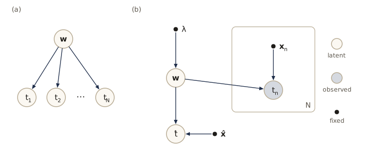
\[p(\mathbf{t}, \mathbf{w} \mid \mathbf{X}, \lambda) = p(\mathbf{w} \mid \lambda) \prod_{n=1}^{N} p(t_n \mid \mathbf{w}, \mathbf{x}_n), \qquad p(\mathbf{w} \mid \lambda) = \mathcal{N}(\mathbf{w} \mid \mathbf{0}, \lambda\mathbf{I}).\]Drawn literally, the graph has a node for \(\mathbf{w}\) with \(N\) arrows to the nodes \(t_1, \dots, t_N\). Writing \(N\) nodes is clumsy, so we use a plate: a box around one representative node \(t_n\), labeled \(N\), meaning “\(N\) copies of whatever is inside, one per \(n\)”. Arrows that cross into the plate go to every copy.
Parameters and observations
Panel (b) of the figure uses three conventions that we keep for the rest of the course.
- An open circle is a random variable we have not observed. An unobserved variable of interest is a latent variable or hidden variable; here \(\mathbf{w}\) and the prediction \(\hat{t}\) are latent.
- A shaded circle is a random variable set to an observed value, here the training targets \(t_n\).
- A small dot is a deterministic parameter: a fixed quantity with no distribution, such as \(\lambda\) or an input \(\mathbf{x}_n\).
For a new input \(\hat{\mathbf{x}}\) the joint distribution of all random variables is
\[p(\hat{t}, \mathbf{t}, \mathbf{w} \mid \hat{\mathbf{x}}, \mathbf{X}, \lambda) = p(\mathbf{w} \mid \lambda)\, p(\hat{t} \mid \mathbf{w}, \hat{\mathbf{x}}) \prod_{n=1}^{N} p(t_n \mid \mathbf{w}, \mathbf{x}_n),\]and the prediction we want is \(p(\hat{t} \mid \hat{\mathbf{x}}, \mathbf{t}, \mathbf{X}, \lambda)\), which the sum rule gives by integrating \(\mathbf{w}\) out against its posterior. For a deep network that integral is out of reach, and in practice we find the single most probable weight vector \(\mathbf{w}_{\mathrm{MAP}}\) and predict with \(p(\hat{t} \mid \mathbf{w}_{\mathrm{MAP}}, \hat{\mathbf{x}})\), as in module 02. With only two weights we can do both on a grid and see the difference. The graph tells us exactly what to compute: the log joint is the log prior plus one log-likelihood term per plate copy.
x_cls = rng.uniform(-2, 2, 10)
t_cls = (rng.random(10) < expit(-0.5 + 2.0 * x_cls)).astype(float)   # true w = (-0.5, 2.0)
lam = 4.0                                                             # prior variance

g = np.linspace(-8, 8, 321)
W0, W1 = np.meshgrid(g, g, indexing="ij")                            # grid over (w0, w1)
A = W0[..., None] + W1[..., None] * x_cls                            # activations, (321, 321, N)
log_joint = (-(W0 ** 2 + W1 ** 2) / (2 * lam)                        # ln p(w | lambda) + ...
             + np.sum(t_cls * -np.logaddexp(0, -A) + (1 - t_cls) * -np.logaddexp(0, A), axis=-1))
post = np.exp(log_joint - logsumexp(log_joint))                      # posterior on the grid
i, j = np.unravel_index(post.argmax(), post.shape)
print(f"w_MAP = ({g[i]:.2f}, {g[j]:.2f})")
print(" x_hat   p(t=1) with w_MAP   p(t=1) averaged over the posterior")
for xh in [-4.0, -1.0, 0.0, 1.0, 4.0]:
    bayes = np.sum(post * expit(W0 + W1 * xh))
    print(f"{xh:5.1f}   {expit(g[i] + g[j] * xh):12.3f}   {bayes:20.3f}")
w_MAP = (-1.15, 2.25)
 x_hat   p(t=1) with w_MAP   p(t=1) averaged over the posterior
 -4.0          0.000                  0.003
 -1.0          0.032                  0.042
  0.0          0.240                  0.259
  1.0          0.750                  0.739
  4.0          1.000                  0.983
Near the data the two predictions are close. Far from the data the plug-in prediction becomes very confident, while the Bayesian average stays more cautious, because it also counts the many weight vectors that fit ten points almost as well as \(\mathbf{w}_{\mathrm{MAP}}\). Intro to ML, module 04 develops the Laplace approximation that makes this averaging practical for larger models.
Bayes’ theorem on a graph
Observing some variables changes the distribution of the others; computing the new distributions is called inference. The smallest example is the graph \(x \to y\) with joint \(p(x)\,p(y \mid x)\). When \(y\) is observed, the sum rule gives \(p(y) = \sum_{x'} p(y \mid x')\, p(x')\) and Bayes’ theorem gives the posterior
\[p(x \mid y) = \frac{p(y \mid x)\, p(x)}{p(y)}.\]Now the same joint is written as \(p(y)\, p(x \mid y)\), the graph \(y \to x\). Inference reverses the arrow.
p_x = np.array([0.5, 0.3, 0.2])                     # three states of x
p_y_x = np.array([[0.9, 0.1], [0.4, 0.6], [0.2, 0.8]])  # p(y | x), rows x
joint_xy = p_x[:, None] * p_y_x                      # graph x -> y
p_y = joint_xy.sum(0)
p_x_y = joint_xy / p_y                               # Bayes' theorem, columns y
print("p(x | y = 1) =", p_x_y[:, 1])
print(f"joint rebuilt from the reversed graph y -> x: max difference "
      f"{np.abs(p_y[None, :] * p_x_y - joint_xy).max():.1e}")
p(x | y = 1) = [0.1282 0.4615 0.4103]
joint rebuilt from the reversed graph y -> x: max difference 6.9e-18
For a large graph, inference is still just the sum and product rules, but doing the sums naively costs time exponential in the number of variables. Exact message-passing algorithms exploit the graph to make it efficient on trees and chains; see Intro to ML, module 08. When the conditionals are neural networks, the reversed conditional \(p(\text{latent} \mid \text{data})\) has no closed form at all. Deep generative models then train a second network to approximate it, which is the encoder of a variational autoencoder in module 19.
Conditional independence
Variables \(a\) and \(b\) are conditionally independent given \(c\) if
\[p(a \mid b, c) = p(a \mid c), \quad \text{equivalently} \quad p(a, b \mid c) = p(a \mid c)\, p(b \mid c),\]for every value of \(c\) (the equivalence is one line of the product rule). We write \(a \perp\!\!\!\perp b \mid c\). Once \(c\) is known, \(b\) tells us nothing more about \(a\). Conditional independence makes models smaller and computations cheaper, and a graph lets us read it off directly.
To check such statements numerically we use the conditional mutual information
\[\mathrm{I}[a; b \mid c] = \sum_{a, b, c} p(a, b, c) \ln \frac{p(a, b \mid c)}{p(a \mid c)\, p(b \mid c)},\]the mutual information of module 02 averaged over \(c\). It is a KL divergence, so it is never negative, and it is zero exactly when \(a \perp\!\!\!\perp b \mid c\). With an empty \(c\) it is the ordinary mutual information.
def cmi(P, order, A, B, C=()):
    """I[A; B | C] in nats from a joint table P whose axes follow `order`."""
    axis = {v: i for i, v in enumerate(order)}
    sub = np.einsum(P, list(range(P.ndim)), [axis[v] for v in (*A, *B, *C)])
    sA = int(np.prod(sub.shape[:len(A)]))
    sB = int(np.prod(sub.shape[len(A):len(A) + len(B)]))
    pabc = sub.reshape(sA, sB, -1)
    pac, pbc, pc = pabc.sum(1, keepdims=True), pabc.sum(0, keepdims=True), pabc.sum((0, 1))
    ratio = np.where(pabc > 0, pabc * pc / (pac * pbc + 1e-300), 1.0)
    return max(float(np.sum(pabc * np.log(ratio))), 0.0)      # round-off can dip below zero
Three example graphs
Three graphs over three variables contain everything we need. In each, the question is whether \(a\) and \(b\) are independent, first with nothing observed and then with \(c\) observed. Relative to the path \(a - c - b\), the node \(c\) is tail-to-tail if both arrows leave it (\(a \leftarrow c \rightarrow b\)), head-to-tail if one arrow enters and one leaves (\(a \rightarrow c \rightarrow b\)), and head-to-head if both enter (\(a \rightarrow c \leftarrow b\)).
Tail-to-tail. The joint is \(p(a, b, c) = p(a \mid c)\, p(b \mid c)\, p(c)\). Summing out \(c\) gives \(p(a, b) = \sum_c p(a \mid c)\, p(b \mid c)\, p(c)\), which in general does not factorize: a common cause makes its effects dependent. Dividing by \(p(c)\) instead gives \(p(a, b \mid c) = p(a \mid c)\, p(b \mid c)\), so \(a \perp\!\!\!\perp b \mid c\).
Head-to-tail. The joint is \(p(a)\, p(c \mid a)\, p(b \mid c)\). Summing out \(c\) gives \(p(a)\, p(b \mid a)\), which in general does not factorize. Given \(c\), Bayes’ theorem turns \(p(a)\, p(c \mid a)\) into \(p(c)\, p(a \mid c)\), so \(p(a, b \mid c) = p(a \mid c)\, p(b \mid c)\) and again \(a \perp\!\!\!\perp b \mid c\). An intermediate step, once known, cuts the chain.
Head-to-head. The joint is \(p(a)\, p(b)\, p(c \mid a, b)\). Summing out \(c\) gives \(p(a)\, p(b)\) exactly, so \(a \perp\!\!\!\perp b\) with nothing observed. But \(p(a, b \mid c) = p(a)\, p(b)\, p(c \mid a, b)/p(c)\), which in general does not factorize, so observing \(c\) makes \(a\) and \(b\) dependent. A head-to-head node is also called a collider. The same happens if we observe any descendant of \(c\), a node reachable from \(c\) by following arrows: a noisy report of the effect is still evidence about the effect.
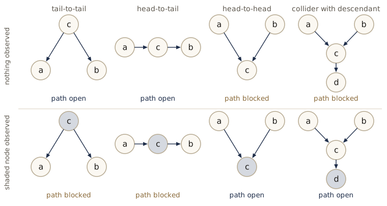
We now check all of this with our own tables. Each graph gets its own CPTs; for the collider we add a child \(d\) of \(c\).
def bern(p1):
    """CPT of a binary variable from p(x = 1), given for each parent setting."""
    p1 = np.asarray(p1, dtype=float)
    return np.stack([1 - p1, p1], axis=-1)

three = {
    "tail-to-tail": ({"c": (), "a": ("c",), "b": ("c",)},
                     {"c": bern(0.4), "a": bern([0.2, 0.7]), "b": bern([0.3, 0.9])}),
    "head-to-tail": ({"a": (), "c": ("a",), "b": ("c",)},
                     {"a": bern(0.35), "c": bern([0.1, 0.8]), "b": bern([0.25, 0.75])}),
    "head-to-head": ({"a": (), "b": (), "c": ("a", "b"), "d": ("c",)},
                     {"a": bern(0.5), "b": bern(0.3), "c": bern([[0.05, 0.6], [0.7, 0.95]]),
                      "d": bern([0.1, 0.85])}),
}
print(f"{'graph':14s} {'I[a;b]':>9s} {'I[a;b|c]':>9s} {'I[a;b|d]':>9s}")
for name, (pa, cp) in three.items():
    od = topological_order(pa)
    Pj = joint_table(pa, cp, od)
    row = f"{name:14s} {cmi(Pj, od, ['a'], ['b']):9.5f} {cmi(Pj, od, ['a'], ['b'], ['c']):9.5f}"
    if "d" in pa:
        row += f" {cmi(Pj, od, ['a'], ['b'], ['d']):9.5f}"
    print(row)
graph             I[a;b]  I[a;b|c]  I[a;b|d]
tail-to-tail     0.04459   0.00000
head-to-tail     0.05742   0.00000
head-to-head     0.00000   0.04277   0.01440
The zeros are exact (up to round-off) and follow from the graphs; the nonzero values depend on our particular numbers. For the first two graphs, dependence disappears when \(c\) is observed. For the collider it is the other way around, and observing only the descendant \(d\) creates a weaker dependence than observing \(c\) itself, since \(d\) is a noisy copy of \(c\).
Explaining away
The collider behavior deserves an example with a story, because it runs against intuition. You start a training run and a while later the loss becomes NaN. Two causes are common: the learning rate was set too high (\(L = 1\)), or the data pipeline has a bug that produces a corrupted batch (\(B = 1\)). Before the run the two are unrelated. The divergence (\(N = 1\)) depends on both, and a monitoring alert (\(A = 1\)) usually fires when the loss diverges. Our made-up numbers: \(p(L = 1) = 0.2\), \(p(B = 1) = 0.05\), and
| \(B = 0\) | \(B = 1\) | |
|---|---|---|
| \(p(N = 1 \mid L = 0, B)\) | 0.02 | 0.80 |
| \(p(N = 1 \mid L = 1, B)\) | 0.60 | 0.95 |
with \(p(A = 1 \mid N = 0) = 0.03\) and \(p(A = 1 \mid N = 1) = 0.97\). What is the probability of a data bug as the evidence comes in?
debug_parents = {"L": (), "B": (), "N": ("L", "B"), "A": ("N",)}
debug_cpts = {"L": bern(0.2), "B": bern(0.05),
              "N": bern([[0.02, 0.80], [0.60, 0.95]]),       # rows L, columns B
              "A": bern([0.03, 0.97])}
debug_order = ["L", "B", "N", "A"]
PD = joint_table(debug_parents, debug_cpts, debug_order)        # axes (L, B, N, A)

def p_bug(**evidence):
    """p(B = 1 | evidence) by summing the joint table."""
    ax = {v: i for i, v in enumerate(debug_order)}
    idx = [slice(None)] * 4
    for v, val in evidence.items():
        idx[ax[v]] = val
    Q = PD[tuple(idx)]
    b_axis = sum(1 for v in debug_order[:1] if v not in evidence)   # position of B in Q
    return Q.take(1, axis=b_axis).sum() / Q.sum()

print(f"p(B=1)                 = {p_bug():.3f}")
print(f"p(B=1 | N=1)           = {p_bug(N=1):.3f}")
print(f"p(B=1 | N=1, L=1)      = {p_bug(N=1, L=1):.3f}")
print(f"p(B=1 | N=1, L=0)      = {p_bug(N=1, L=0):.3f}")
print(f"p(B=1 | A=1)           = {p_bug(A=1):.3f}")
print(f"p(B=1 | A=1, L=1)      = {p_bug(A=1, L=1):.3f}")
print(f"I[L;B] = {cmi(PD, debug_order, ['L'], ['B']):.1e}   "
      f"I[L;B|N] = {cmi(PD, debug_order, ['L'], ['B'], ['N']):.4f}   "
      f"I[L;B|A] = {cmi(PD, debug_order, ['L'], ['B'], ['A']):.4f}")
p(B=1)                 = 0.050
p(B=1 | N=1)           = 0.243
p(B=1 | N=1, L=1)      = 0.077
p(B=1 | N=1, L=0)      = 0.678
p(B=1 | A=1)           = 0.213
p(B=1 | A=1, L=1)      = 0.076
I[L;B] = 0.0e+00   I[L;B|N] = 0.0316   I[L;B|A] = 0.0187
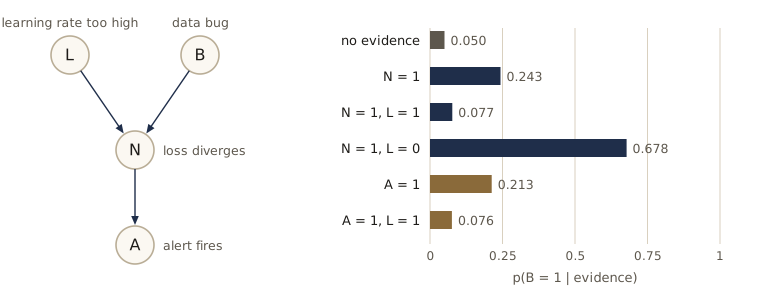
The divergence alone raises the probability of a data bug from 5% to about a quarter, because a bug is one of the two ways to get a NaN. Then you look at the config and find the learning rate was far too high. Nothing about the data has changed, yet the bug probability drops back close to its prior: the learning rate explains away the divergence. If instead the learning rate turns out to be fine, the bug becomes the likely culprit. So \(L\) and \(B\), independent before the run, became dependent once we saw their common effect. Seeing only the alert, a descendant of \(N\), gives the same pattern slightly weaker, just as the head-to-head rule said.
Watch out. Conditioning can create dependence. Selecting data on an outcome (only the runs that diverged, only the patients admitted to a hospital) makes the outcome’s causes look correlated even when they are independent in the population. In a generative model it means that latent causes which are independent a priori are coupled in the posterior, which is why the posterior of a VAE or of the image model below is hard to compute.
D-separation
For larger graphs we need a rule that applies to any path. Let \(A\), \(B\), \(C\) be disjoint sets of nodes. A path is a sequence of distinct nodes joined by links, taken in either direction.
Definition. A path from a node in \(A\) to a node in \(B\) is blocked by \(C\) if it passes through a node where either
- the arrows meet head-to-tail or tail-to-tail, and the node is in \(C\); or
- the arrows meet head-to-head, and neither the node itself nor any descendant of it is in \(C\).
If every such path is blocked, \(A\) is d-separated from \(B\) by \(C\), and then \(A \perp\!\!\!\perp B \mid C\) holds for every distribution that factorizes according to the graph.
The “d” stands for “directed”. The criterion is due to Judea Pearl; a proof that it is correct can be found in Lauritzen’s book on graphical models. On our running example: \(x_1 \perp\!\!\!\perp x_2\), since their only connections meet head-to-head at \(x_3\) or further down; but conditioning on \(x_7\), a descendant of \(x_3\), opens the collider. And \(x_3 \perp\!\!\!\perp x_6 \mid x_4\), since \(x_4\) blocks \(x_3 \leftarrow x_2 \rightarrow x_4 \rightarrow x_6\) and \(x_3 \rightarrow x_5 \leftarrow x_4 \rightarrow x_6\), while \(x_3 \rightarrow x_5 \rightarrow x_7 \leftarrow x_6\) is blocked by the unobserved collider \(x_7\). Add \(x_7\) to the conditioning set and that last path opens.
We implement the criterion twice. The first version follows the definition literally: list every path and test every node on it. That is fine for seven nodes, but the number of paths can grow exponentially with the size of the graph. The second version is a reachability search, often called the Bayes ball: a ball starts at the nodes of \(A\) and travels along links, in either direction, as long as the three rules let it pass, and \(A\) is d-separated from \(B\) exactly when the ball never reaches \(B\). The only state the ball needs is which node it is at and whether it arrived from a child (moving “up”, against an arrow) or from a parent (moving “down”, along an arrow). The rules at a node \(v\) are the three example graphs again:
- Arriving from a child, the ball can continue to \(v\)’s parents (head-to-tail) and to its other children (tail-to-tail), but only if \(v \notin C\).
- Arriving from a parent, it can continue to \(v\)’s children (head-to-tail) if \(v \notin C\), and bounce back up to \(v\)’s other parents (head-to-head) only if \(v\) or one of its descendants is in \(C\), that is, if \(v\) is in \(C\) or is an ancestor of a node in \(C\).
Each (node, direction) pair is visited at most once, so the search takes time linear in the size of the graph. Intro to ML, module 08 walks through the same search on its own examples.
def children_of(parents):
    ch = {v: [] for v in parents}
    for v, pa in parents.items():
        for u in pa:
            ch[u].append(v)
    return ch

def descendants(parents, v):
    ch, out, stack = children_of(parents), set(), [v]
    while stack:
        for c in ch[stack.pop()]:
            if c not in out:
                out.add(c)
                stack.append(c)
    return out

def all_paths(parents, a, b):
    """Every simple path from a to b, ignoring arrow directions."""
    ch = children_of(parents)
    nbrs = {v: set(parents[v]) | set(ch[v]) for v in parents}
    stack = [[a]]
    while stack:
        path = stack.pop()
        for w in nbrs[path[-1]]:
            if w == b:
                yield path + [w]
            elif w not in path:
                stack.append(path + [w])

def blocked(parents, path, C):
    for prev, node, nxt in zip(path, path[1:], path[2:]):
        if prev in parents[node] and nxt in parents[node]:        # head-to-head at node
            if node not in C and not (descendants(parents, node) & C):
                return True
        elif node in C:                                            # head-to-tail or tail-to-tail
            return True
    return False

def d_separated(parents, A, B, C=()):
    C = set(C)
    return all(blocked(parents, p, C) for a in A for b in B for p in all_paths(parents, a, b))

def bayes_ball(parents, A, B, C=()):
    """Reachability search over (node, direction) pairs; True if A and B are d-separated by C."""
    C, ch = set(C), children_of(parents)
    anc_C, stack = set(), list(C)                 # C and its ancestors: colliders there are open
    while stack:
        v = stack.pop()
        if v not in anc_C:
            anc_C.add(v)
            stack.extend(parents[v])
    visited, reached = set(), set()
    stack = [(a, "up") for a in A]                # "up" = arrived from a child (or the start)
    while stack:
        v, d = stack.pop()
        if (v, d) in visited:
            continue
        visited.add((v, d))
        if v not in C:
            reached.add(v)
        if d == "up" and v not in C:               # on to parents and to the other children
            stack += [(u, "up") for u in parents[v]] + [(w, "down") for w in ch[v]]
        elif d == "down":
            if v not in C:                         # head-to-tail: on to the children
                stack += [(w, "down") for w in ch[v]]
            if v in anc_C:                         # head-to-head, opened by v or a descendant
                stack += [(u, "up") for u in parents[v]]
    return not (reached & set(B))

for A_, B_, C_ in [("x1", "x2", ()), ("x1", "x2", ("x7",)), ("x3", "x6", ("x4",)),
                   ("x3", "x6", ("x4", "x7")), ("x1", "x7", ("x5",))]:
    given = "{" + ",".join(C_) + "}"
    print(f"{A_} vs {B_} given {given}: d-separated "
          f"{d_separated(parents, [A_], [B_], C_)!s:5s} (Bayes ball: "
          f"{bayes_ball(parents, [A_], [B_], C_)!s:5s})  "
          f"I = {cmi(P, order, [A_], [B_], C_):.1e}")
x1 vs x2 given {}: d-separated True  (Bayes ball: True )  I = 0.0e+00
x1 vs x2 given {x7}: d-separated False (Bayes ball: False)  I = 8.7e-06
x3 vs x6 given {x4}: d-separated True  (Bayes ball: True )  I = 5.6e-17
x3 vs x6 given {x4,x7}: d-separated False (Bayes ball: False)  I = 8.6e-05
x1 vs x7 given {x5}: d-separated False (Bayes ball: False)  I = 3.2e-06
Every “True” comes with a mutual information at round-off level, every “False” with a positive one. The last query is worth tracing. The direct route \(x_1 \rightarrow x_3 \rightarrow x_5 \rightarrow x_7\) is blocked at the observed, head-to-tail \(x_5\). But \(x_5\) is a descendant of the collider \(x_3\), so observing it opens \(x_1 \rightarrow x_3 \leftarrow x_2 \rightarrow x_4 \rightarrow x_6 \rightarrow x_7\), and \(x_1\) still carries information about \(x_7\). The real test is exhaustive: every pair of nodes and every conditioning set drawn from the other five, on the running example and on random DAGs with random CPTs, compared with the brute-force conditional mutual information.
def random_dag(n, p_edge, rng, max_parents=3):
    names = [f"x{i}" for i in range(1, n + 1)]            # numbering = a topological order
    return {v: tuple(u for u in names[:i] if rng.random() < p_edge)[:max_parents]
            for i, v in enumerate(names)}

def check_graph(pa, Pj, od):
    n_q = n_sep = n_bad = 0
    largest_sep, smallest_dep = 0.0, np.inf
    for a, b in combinations(od, 2):
        rest = [u for u in od if u not in (a, b)]
        for r in range(len(rest) + 1):
            for C in combinations(rest, r):
                sep = d_separated(pa, [a], [b], C)
                n_bad += sep != bayes_ball(pa, [a], [b], C)
                I = cmi(Pj, od, [a], [b], C)
                n_q += 1
                n_sep += sep
                n_bad += sep != (I < 1e-12)
                if sep:
                    largest_sep = max(largest_sep, I)
                else:
                    smallest_dep = min(smallest_dep, I)
    return np.array([n_q, n_sep, n_bad]), largest_sep, smallest_dep

tot, big, small = check_graph(parents, P, order)
print(f"running example: {tot[0]} queries, {tot[1]} d-separated, {tot[2]} disagreements")
tot, big, small = np.zeros(3, int), 0.0, np.inf
for _ in range(10):
    pa_r = random_dag(7, 0.4, rng)
    od_r = topological_order(pa_r)
    states_r = {u: int(rng.integers(2, 4)) for u in pa_r}          # 2 or 3 states per node
    P_r = joint_table(pa_r, random_cpts(pa_r, states_r, rng), od_r)
    t_, b_, s_ = check_graph(pa_r, P_r, od_r)
    tot, big, small = tot + t_, max(big, b_), min(small, s_)
print(f"10 random DAGs: {tot[0]} queries, {tot[1]} d-separated, {tot[2]} disagreements")
print(f"largest I when d-separated {big:.1e}; smallest I when not {small:.1e}")
running example: 672 queries, 151 d-separated, 0 disagreements
10 random DAGs: 6720 queries, 2379 d-separated, 0 disagreements
largest I when d-separated 2.2e-16; smallest I when not 9.2e-10
The two implementations agree with each other and with brute force on every query. The comparison works in one direction by theory and in the other by luck we can quantify. D-separation guarantees independence. When a path is open, the graph permits dependence, but special numbers in the CPTs could still cancel it; with CPTs drawn at random such cancellations happen with probability zero, which is why the brute-force test finds a dependence every time.
Two consequences are used constantly. First, deterministic parameters such as \(\lambda\) behave like observed nodes, and since they have no parents every path through them is tail-to-tail and blocked: they never create dependence. Second, look at the classifier graph. Every path from \(\hat{t}\) to a training target \(t_n\) passes tail-to-tail through \(\mathbf{w}\), so
\[\hat{t} \perp\!\!\!\perp t_n \mid \mathbf{w}.\]Given the weights, the training data carry no further information about the prediction. This is what allows us to train a network, throw the training set away, and predict from the weights alone. It is also why data points are called independent and identically distributed: they are independent given the parameters. With the parameters unknown, the path through \(\mathbf{w}\) is open, and the targets are dependent, which is exactly why observing some of them tells us something about the others.
Naive Bayes
The naive Bayes model is a classifier built on a tail-to-tail structure. The class label \(\mathcal{C}_k\) is the parent of every component of the input \(\mathbf{x} = (x^{(1)}, \dots, x^{(L)})\), and nothing else is linked:
\[p(\mathbf{x} \mid \mathcal{C}_k) = \prod_{l=1}^{L} p(x^{(l)} \mid \mathcal{C}_k).\]Given the class, the components are independent, because every path between them is tail-to-tail at \(\mathcal{C}_k\). Without the class, the paths are open, and the marginal \(p(\mathbf{x}) = \sum_k p(\mathbf{x} \mid \mathcal{C}_k)\, p(\mathcal{C}_k)\) does not factorize. Fitting is easy: with independent parameters for each factor, maximum likelihood fits each one-dimensional density separately, class by class, and sets \(p(\mathcal{C}_k)\) to the fraction of training points in class \(k\). Classification uses Bayes’ theorem, \(p(\mathcal{C}_k \mid \mathbf{x}) \propto p(\mathbf{x} \mid \mathcal{C}_k)\, p(\mathcal{C}_k)\). The factors can be of different kinds, a Bernoulli for a binary feature and a Gaussian for a real one, which makes the model convenient for mixed data. The same factorization is how Bishop & Bishop §5.2.4 combine two sources of evidence that are independent given the class.
The independence assumption is usually false. Is the model still useful? We generate two Gaussian classes whose features are correlated (correlation 0.5 between every pair), so the naive assumption is wrong, and compare naive Bayes (a diagonal Gaussian per class) with a full-covariance Gaussian per class.
def correlated_classes(D, n, rng, rho=0.5):
    Lc = np.linalg.cholesky((1 - rho) * np.eye(D) + rho * np.ones((D, D)))
    t = rng.integers(0, 2, n)
    X = rng.standard_normal((n, D)) @ Lc.T + t[:, None] * np.linspace(1, -0.5, D)
    return X, t

def fit_gaussian_classes(X, t, naive):
    model = []
    for k in (0, 1):
        Xk = X[t == k]
        S_k = np.cov(Xk.T, bias=True).reshape(X.shape[1], X.shape[1])
        model.append((Xk.mean(0), np.diag(np.diag(S_k)) if naive else S_k, np.mean(t == k)))
    return model

def predict_classes(model, X):
    scores = []
    for m, S_k, pi in model:                                  # ln N(x | m, S) + ln p(C_k)
        Lc = np.linalg.cholesky(S_k)
        z = np.linalg.solve(Lc, (X - m).T)
        scores.append(-0.5 * (z ** 2).sum(0) - np.log(np.diag(Lc)).sum() + np.log(pi))
    return np.argmax(scores, axis=0)

print(" D     N   naive Bayes   full covariance   (mean test accuracy over 10 data sets)")
for D_nb, N_nb in [(2, 200), (40, 120), (40, 2000)]:
    acc = np.zeros(2)
    for _ in range(10):
        X, t = correlated_classes(D_nb, N_nb, rng)
        Xt, tt = correlated_classes(D_nb, 5000, rng)
        acc += [np.mean(predict_classes(fit_gaussian_classes(X, t, nv), Xt) == tt) / 10
                for nv in (True, False)]
    print(f"{D_nb:2d} {N_nb:5d}   {acc[0]:10.3f}   {acc[1]:14.3f}")
 D     N   naive Bayes   full covariance   (mean test accuracy over 10 data sets)
 2   200        0.756            0.774
40   120        0.803            0.661
40  2000        0.764            0.969
In two dimensions the wrong assumption costs about two points of accuracy. In 40 dimensions with 120 examples, about 60 per class, naive Bayes wins: the full model has to estimate 820 covariance entries per class from 60 points, and its estimates are too noisy to help. With 2000 examples the full model can estimate the correlations and wins by a wide margin. Naive Bayes is a strong baseline when the dimension is high relative to the data, and it is a reminder that a model with a false independence assumption can still classify well.
Even though each class density factorizes, the marginal does not. With class means \(\boldsymbol{\mu}_k\), diagonal covariances \(\boldsymbol{\Sigma}_k\) and priors \(\pi_k\), the mixture has covariance \(\sum_k \pi_k(\boldsymbol{\Sigma}_k + \boldsymbol{\mu}_k\boldsymbol{\mu}_k^{\mathrm{T}}) - \bar{\boldsymbol{\mu}}\bar{\boldsymbol{\mu}}^{\mathrm{T}}\) with \(\bar{\boldsymbol{\mu}} = \sum_k \pi_k \boldsymbol{\mu}_k\), whose off-diagonal entries are nonzero whenever the class means differ in both coordinates:
nb = [(np.array([0.0, 0.0]), np.diag([1.0, 0.5]), 0.5),
      (np.array([2.0, 1.5]), np.diag([0.6, 1.0]), 0.5)]
mbar = sum(pi * m for m, _, pi in nb)
cov_mix = sum(pi * (S_k + np.outer(m, m)) for m, S_k, pi in nb) - np.outer(mbar, mbar)
k_s = rng.integers(0, 2, 200_000)
Xm = np.stack([nb[k][0] for k in (0, 1)])[k_s] + rng.standard_normal((200_000, 2)) * np.sqrt(
    np.stack([np.diag(nb[k][1]) for k in (0, 1)])[k_s])
print("covariance of p(x), formula:\n", cov_mix)
print("covariance of p(x), samples:\n", np.cov(Xm.T))
covariance of p(x), formula:
 [[1.8    0.75  ]
 [0.75   1.3125]]
covariance of p(x), samples:
 [[1.7915 0.7525]
 [0.7525 1.3174]]
Generative models
Many learning problems are inverse problems. An image of an object is produced by a physical process: an object of some class is placed at some position, at some scale, and light forms the image. Recognition runs the process backwards. One approach trains a network to map images directly to class, position, and scale; that is a discriminative model, and it needs labeled images. The other approach models the forward process, image given its causes, and then inverts it with Bayes’ theorem; that is a generative model. Its graph has class, position, and scale as independent parents of the image, and the arrows follow the order in which the data are produced.
A generative model can also make new data. Ancestral sampling draws the variables in a topological order, each from its conditional given the already-drawn values of its parents. Every sample is an exact draw from the joint distribution, and no normalization or inference is needed. Here it is on the running example, compared with the exact joint table:
def ancestral_sample(parents, cpts, order, n, rng):
    """n joint samples: visit nodes in topological order, draw each given its sampled parents."""
    x = {}
    for v in order:
        probs = cpts[v][tuple(x[u] for u in parents[v])]           # (n, K) or (K,) for a root
        probs = np.broadcast_to(probs, (n, probs.shape[-1]))
        u = rng.random((n, 1))
        x[v] = np.minimum((u > probs.cumsum(axis=1)).sum(axis=1), probs.shape[-1] - 1)
    return x

xs = ancestral_sample(parents, cpts, order, 200_000, rng)
exact = [P.sum(axis=tuple(j for j in range(7) if j != i))[1] for i in range(7)]
print("node   exact p(x=1)   sampled")
for i, v in enumerate(order):
    print(f"{v:4s}   {exact[i]:10.4f}   {xs[v].mean():8.4f}")
p37 = P.sum(axis=tuple(j for j, u in enumerate(order) if u not in ("x3", "x7")))
print(f"p(x3=1, x7=1): exact {p37[1, 1]:.4f}, "
      f"sampled {np.mean((xs['x3'] == 1) & (xs['x7'] == 1)):.4f}")
node   exact p(x=1)   sampled
x1         0.2675     0.2688
x2         0.2330     0.2316
x3         0.5700     0.5695
x4         0.2861     0.2865
x5         0.5189     0.5170
x6         0.8012     0.8000
x7         0.4840     0.4838
p(x3=1, x7=1): exact 0.2812, sampled 0.2809
Now a small version of the object-in-an-image example, with a one-dimensional “image” of 24 pixels. The latent class is either a single bump or a pair of bumps six pixels apart, the latent position \(s\) is the center, and each pixel gets Gaussian noise. Class and position are independent a priori (their paths meet head-to-head at the image). We generate one image from a pair centered at pixel 12 and compute the exact posterior over (class, position) by enumerating all 36 combinations.
u_pix = np.arange(24)
positions = np.arange(3, 21)
sigma_pix = 0.6

def render(k, s):
    """Mean image: class 0 = one bump at s, class 1 = two bumps at s - 3 and s + 3."""
    bump = lambda c: np.exp(-0.5 * (u_pix - c) ** 2)
    return bump(s) if k == 0 else bump(s - 3) + bump(s + 3)

rng_img = np.random.default_rng(3)
image = render(1, 12) + sigma_pix * rng_img.standard_normal(24)
log_post = np.array([[-0.5 * np.sum((image - render(k, s)) ** 2) / sigma_pix ** 2
                      for s in positions] for k in (0, 1)])      # uniform priors cancel
post_ks = np.exp(log_post - logsumexp(log_post))
p_k = post_ks.sum(1)
print(f"p(class = one bump | image) = {p_k[0]:.3f},  p(class = pair | image) = {p_k[1]:.3f}")
for k, name in [(0, "one bump"), (1, "pair")]:
    ps = post_ks[k] / p_k[k]
    print(f"given {name:8s}: most probable position {positions[ps.argmax()]:2d} "
          f"(probability {ps.max():.2f})")
I_post = np.sum(post_ks * np.log(post_ks / np.outer(p_k, post_ks.sum(0)) + 1e-300))
print(f"mutual information of class and position given the image: {I_post:.3f} nats")
p(class = one bump | image) = 0.256,  p(class = pair | image) = 0.744
given one bump: most probable position  9 (probability 0.92)
given pair    : most probable position 12 (probability 0.90)
mutual information of class and position given the image: 0.568 nats
The answer to “where is the object?” depends on what the object is. If it is a single bump, it must be the strong bump near pixel 9; if it is a pair, it is centered at 12. Class and position, independent before we looked, are strongly dependent after, which is explaining away again. Deep generative models are built the same way, with one change: their latent variables are usually not interpretable quantities such as class or position, but vectors drawn from a simple Gaussian, and a neural network maps them to data. Normalizing flows (module 18), variational autoencoders (module 19), and diffusion models (module 20) all sample this way, and the discrete and continuous latent-variable models of module 15 and module 16 are their simpler ancestors.
In practice. Ancestral sampling is cheap for any directed model, however large, so generating data is easy. The hard direction is the reverse, the posterior over the latents given an observation, since all latents that share an observed child become coupled. Much of the machinery of modules 15–20 (EM, variational bounds, amortized encoders) exists to deal with that reverse direction.
Markov blanket
Which variables does a single node \(x_i\) actually depend on, once everything else is known? Write the conditional given all other variables with the factorization, where the sum is an integral for continuous variables:
\[p(x_i \mid \mathbf{x}_{\setminus i}) = \frac{p(x_1, \dots, x_D)}{\sum_{x_i} p(x_1, \dots, x_D)} = \frac{\prod_k p(x_k \mid \mathrm{pa}(k))}{\sum_{x_i} \prod_k p(x_k \mid \mathrm{pa}(k))}.\]Every factor that does not contain \(x_i\) can be pulled out of the sum in the denominator and cancels with the same factor in the numerator. The factors that survive are \(x_i\)’s own conditional \(p(x_i \mid \mathrm{pa}(i))\) and the conditionals \(p(x_k \mid \mathrm{pa}(k))\) of its children, since those are the only ones with \(x_i\) on the right of the bar. They involve three groups of variables: the parents of \(x_i\), its children, and its co-parents, the other parents of its children. Together these form the Markov blanket of \(x_i\):
\[p(x_i \mid \mathbf{x}_{\setminus i}) \propto p(x_i \mid \mathrm{pa}(i)) \prod_{k \in \mathrm{ch}(i)} p(x_k \mid \mathrm{pa}(k)).\]Conditioned on its blanket, a node is independent of every other variable. The co-parents must be included because of explaining away: observing a child opens the path from \(x_i\) to the child’s other parents. We check three things on the running example: conditioning on the blanket of \(x_4\) reproduces the full conditional; dropping the co-parent \(x_3\) does not; and the local product of CPTs on the right-hand side gives the same answer without ever building the joint table.
def markov_blanket(parents, v):
    ch = [c for c, pa in parents.items() if v in pa]
    co = {u for c in ch for u in parents[c]} - {v}
    return set(parents[v]) | set(ch) | co

def conditional(P, order, target, given):
    """p(target | given) laid out on the axes of P (sums out everything else)."""
    axis = {u: i for i, u in enumerate(order)}
    drop = tuple(axis[u] for u in order if u != target and u not in given)
    m = P.sum(axis=drop, keepdims=True)
    return np.broadcast_to(m / m.sum(axis=axis[target], keepdims=True), P.shape)

def on_axes(parents, cpts, order, v):
    """The CPT of v broadcast onto the joint table's axes (size 1 on axes it does not use)."""
    axis = {u: i for i, u in enumerate(order)}
    vs = list(parents[v]) + [v]
    t = np.transpose(cpts[v], np.argsort([axis[u] for u in vs]))
    shape = [1] * len(order)
    for u, n_u in zip(vs, cpts[v].shape):
        shape[axis[u]] = n_u
    return t.reshape(shape)

mb = markov_blanket(parents, "x4")
others = [u for u in order if u != "x4"]
full = conditional(P, order, "x4", others)
local = on_axes(parents, cpts, order, "x4")
for c in (c for c, pa in parents.items() if "x4" in pa):
    local = local * on_axes(parents, cpts, order, c)
local = np.broadcast_to(local / local.sum(axis=order.index("x4"), keepdims=True), P.shape)
print("Markov blanket of x4:", sorted(mb))
print(f"p(x4 | all others) vs p(x4 | blanket):             "
      f"{np.abs(full - conditional(P, order, 'x4', mb)).max():.1e}")
print(f"p(x4 | all others) vs p(x4 | parents, children):   "
      f"{np.abs(full - conditional(P, order, 'x4', {'x2', 'x5', 'x6'})).max():.1e}")
print(f"p(x4 | all others) vs product of the local CPTs:   {np.abs(full - local).max():.1e}")
Markov blanket of x4: ['x2', 'x3', 'x5', 'x6']
p(x4 | all others) vs p(x4 | blanket):             2.2e-16
p(x4 | all others) vs p(x4 | parents, children):   5.3e-02
p(x4 | all others) vs product of the local CPTs:   2.2e-16
For Gaussian nodes the blanket shows up in the precision matrix \(\boldsymbol{\Lambda} = \boldsymbol{\Sigma}^{-1}\). From the matrix form of the linear-Gaussian model, \(\boldsymbol{\Lambda} = (\mathbf{I} - \mathbf{W})^{\mathrm{T}}\mathbf{V}^{-1}(\mathbf{I} - \mathbf{W})\), and the conditioning formula of module 03 says that the pair \((x_i, x_j)\), given all the other variables, has as its precision the \(2 \times 2\) block of \(\boldsymbol{\Lambda}\) in rows and columns \(i, j\). That block is diagonal, and the pair conditionally independent, exactly when \(\Lambda_{ij} = 0\). So the nonzero pattern of \(\boldsymbol{\Lambda}\) should list, for each node, its Markov blanket:
Lam = np.linalg.inv(S)
offdiag = (np.abs(Lam) > 1e-9) & ~np.eye(D, dtype=bool)
blanket = np.array([[a != c and c in markov_blanket(parents, a) for c in order] for a in order])
print("order:", order)
print("off-diagonal nonzeros of the precision matrix:\n", offdiag.astype(int))
print("same pattern as the Markov blankets:", np.array_equal(offdiag, blanket))
order: ['x1', 'x2', 'x3', 'x4', 'x5', 'x6', 'x7']
off-diagonal nonzeros of the precision matrix:
 [[0 1 1 0 0 0 0]
 [1 0 1 1 0 0 0]
 [1 1 0 1 1 0 0]
 [0 1 1 0 1 1 0]
 [0 0 1 1 0 1 1]
 [0 0 0 1 1 0 1]
 [0 0 0 0 1 1 0]]
same pattern as the Markov blankets: True
The Markov blanket is what makes Gibbs sampling (module 14) cheap: to resample one variable given all the others, we only need the few factors that mention it.
Graphs as filters
A directed graph describes a set of distributions, and it does so in two ways. Think of the graph as a filter. The first filter lets a distribution \(p(\mathbf{x})\) through if it can be written in the factorized form \(\prod_k p(x_k \mid \mathrm{pa}(k))\) for some choice of conditionals; call the set that passes \(\mathcal{DF}\), for directed factorization. The second filter lists every independence statement that d-separation reads off the graph and lets a distribution through if it satisfies all of them. The d-separation theorem says that the two filters pass exactly the same set.
The chain \(a \to c \to b\) is small enough to test both filters by hand. Its only d-separation statement is \(a \perp\!\!\!\perp b \mid c\). For the first filter, a distribution passes if rebuilding it from its own \(p(a)\), \(p(c \mid a)\), and \(p(b \mid c)\) gives it back unchanged.
def rebuild_as_chain(Q):
    """Q has axes (a, c, b): rebuild p(a) p(c | a) p(b | c) from Q's own marginals."""
    p_a, p_ac, p_cb = Q.sum((1, 2)), Q.sum(2), Q.sum(0)
    return (p_a[:, None, None] * (p_ac / p_a[:, None])[:, :, None]
            * (p_cb / p_cb.sum(1, keepdims=True))[None])

chain = {"a": (), "c": ("a",), "b": ("c",)}
collider = {"a": (), "b": (), "c": ("a", "b")}
trials = {
    "random joint": rng.dirichlet(np.ones(8)).reshape(2, 2, 2),
    "from a -> c -> b": joint_table(chain, random_cpts(chain, dict(a=2, b=2, c=2), rng),
                                    ["a", "c", "b"]),
    "from a -> c <- b": joint_table(collider, random_cpts(collider, dict(a=2, b=2, c=2), rng),
                                    ["a", "b", "c"]).transpose(0, 2, 1),
    "fully factorized": np.einsum("i,j,k->ijk", *rng.dirichlet(np.ones(2), size=3)),
}
print(f"{'distribution':18s} {'factorization gap':>18s} {'I[a;b|c]':>10s}")
for name, Q in trials.items():
    print(f"{name:18s} {np.abs(rebuild_as_chain(Q) - Q).max():18.1e} "
          f"{cmi(Q, ['a', 'c', 'b'], ['a'], ['b'], ['c']):10.1e}")
distribution        factorization gap   I[a;b|c]
random joint                  7.4e-02    1.1e-01
from a -> c -> b              3.5e-18    9.4e-18
from a -> c <- b              2.7e-02    2.9e-02
fully factorized              1.4e-17    0.0e+00
The two filters give the same verdict on all four distributions. A fully connected graph passes every distribution, and a graph with no links passes only fully factorized ones. The last row shows the other point worth remembering: a distribution with more independence than the graph requires always passes, so the fully factorized distribution goes through the filter of every graph. A graph states which independences are guaranteed, not which dependences must exist. The theorem also does not care what kind of variables sit at the nodes: the same statements hold for discrete, Gaussian, or neural conditionals.
Sequence models
Text, audio, DNA, and time series are sequences \(\mathbf{x}_1, \dots, \mathbf{x}_N\) with a natural order. (Several independent sequences simply multiply; we model one.) The product rule in the order of the sequence gives
\[p(\mathbf{x}_1, \dots, \mathbf{x}_N) = \prod_{n=1}^{N} p(\mathbf{x}_n \mid \mathbf{x}_1, \dots, \mathbf{x}_{n-1}),\]an autoregressive model: each element is predicted from all the elements before it. As a graph it is fully connected, so on its own it assumes nothing. Models make assumptions by deleting arrows, that is, by shortening the conditioning sets. At the other extreme, deleting all of them gives \(\prod_n p(\mathbf{x}_n)\), which ignores the order entirely.
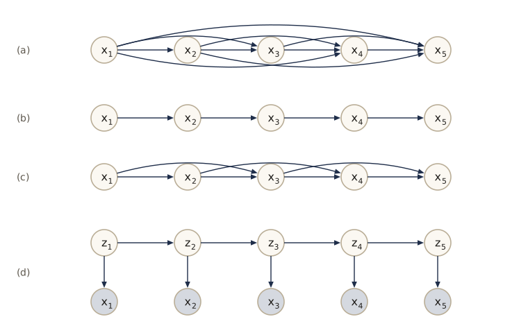
Markov chains
A first-order Markov chain keeps only the previous element:
\[p(\mathbf{x}_1, \dots, \mathbf{x}_N) = p(\mathbf{x}_1) \prod_{n=2}^{N} p(\mathbf{x}_n \mid \mathbf{x}_{n-1}).\]By d-separation, \(\mathbf{x}_{n-1}\) blocks every path from \(\mathbf{x}_n\) to the earlier elements, so \(p(\mathbf{x}_n \mid \mathbf{x}_1, \dots, \mathbf{x}_{n-1}) = p(\mathbf{x}_n \mid \mathbf{x}_{n-1})\): the next prediction depends only on the most recent value. An \(M\)th-order chain conditions each element on the previous \(M\). For discrete elements with \(K\) states and full tables, \(p(x_n \mid x_{n-M}, \dots, x_{n-1})\) needs \(K - 1\) numbers for each of the \(K^M\) contexts, so
\[\text{parameters of an } M\text{th-order chain} = K^{M}(K - 1),\]exponential in the order. For \(M = 1\) it is the \(K(K - 1)\) of a first-order chain. (Bishop & Bishop §11.3 print the exponent as \(M - 1\); counting the contexts, as we just did, gives \(K^M\).) A second-order chain is also a first-order chain over pairs \((x_{n-1}, x_n)\), so higher-order models are no new kind of object. Let us see what this means on real text. We fit character-level Markov chains of order \(M = 0, \dots, 6\) to the first 90% of the Tiny Shakespeare corpus by counting, with a pseudo-count of 0.01 per outcome, and measure the average number of bits per character on the last 10%. Each context of \(M\) characters is encoded as one integer, so counting is a call to np.unique.
path = "data/tinyshakespeare.txt"
if not os.path.exists(path):
    urllib.request.urlretrieve(
        "https://raw.githubusercontent.com/karpathy/char-rnn/master/data/tinyshakespeare/input.txt", path)
text = open(path).read()
chars = sorted(set(text))
K = len(chars)
lut = {c: i for i, c in enumerate(chars)}
seq = np.array([lut[c] for c in text], dtype=np.int64)
split = int(0.9 * len(seq))
train_seq, test_seq = seq[:split], seq[split:]
print(f"{len(seq):,d} characters, K = {K} distinct symbols")

def contexts(s, order_M):
    """Integer code of the order_M preceding symbols, for positions order_M .. len(s) - 1."""
    c = np.zeros(len(s) - order_M, dtype=np.int64)
    for j in range(order_M):
        c = c * K + s[j:len(s) - order_M + j]
    return c

def fit_markov(s, order_M):
    c = contexts(s, order_M)
    pair_keys, pair_n = np.unique(c * K + s[order_M:], return_counts=True)
    ctx_keys, ctx_n = np.unique(c, return_counts=True)
    return pair_keys, pair_n, ctx_keys, ctx_n

def count(keys, n, q):
    i = np.minimum(np.searchsorted(keys, q), len(keys) - 1)
    return np.where(keys[i] == q, n[i], 0)

def bits_per_char(s, model, order_M, alpha=0.01):
    pair_keys, pair_n, ctx_keys, ctx_n = model
    c = contexts(s, order_M)
    n_c = count(ctx_keys, ctx_n, c)
    p = (count(pair_keys, pair_n, c * K + s[order_M:]) + alpha) / (n_c + K * alpha)
    return -np.mean(np.log2(p)), np.mean(n_c == 0)

print("M   parameters K^M(K-1)   contexts seen   train bits   test bits   unseen test contexts")
markov_models = {}
for order_M in range(7):
    markov_models[order_M] = fit_markov(train_seq, order_M)
    tr_bits, _ = bits_per_char(train_seq, markov_models[order_M], order_M)
    te_bits, unseen = bits_per_char(test_seq, markov_models[order_M], order_M)
    print(f"{order_M}   {K ** order_M * (K - 1):19.2e}   {len(markov_models[order_M][2]):13,d}"
          f"   {tr_bits:10.3f}   {te_bits:9.3f}   {unseen:19.1%}")
1,115,394 characters, K = 65 distinct symbols
M   parameters K^M(K-1)   contexts seen   train bits   test bits   unseen test contexts
0              6.40e+01               1        4.774       4.829                  0.0%
1              4.16e+03              65        3.537       3.589                  0.0%
2              2.70e+05           1,380        2.747       2.980                  0.2%
3              1.76e+07          11,228        2.160       2.591                  1.4%
4              1.14e+09          48,539        1.793       2.554                  4.2%
5              7.43e+10         133,293        1.522       2.895                 10.1%
6              4.83e+12         264,623        1.297       3.413                 20.8%
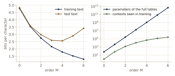
Training loss falls with every added order, but test loss bottoms out around order 4 and then rises: higher-order tables are mostly empty, and at order 6 a fifth of the test contexts never appeared in training, so the model can only fall back on its pseudo-counts. The number of parameters grows like \(65^M\), while the number of contexts that occur in the text grows far more slowly. A table is simply the wrong way to store a long-range conditional. Sampling from the order-4 chain, one character at a time (ancestral sampling along the chain), shows what it has learned:
def sample_markov(models, order_M, prompt, n_chars, rng):
    """Ancestral sampling along the chain; an unseen context is shortened until it has counts."""
    out = [lut[ch] for ch in prompt]
    for _ in range(n_chars):
        for m in range(order_M, -1, -1):                  # back off: M, M - 1, ..., 0
            c = 0
            for sym in out[len(out) - m:] if m > 0 else []:
                c = c * K + sym
            counts = count(models[m][0], models[m][1], c * K + np.arange(K)).astype(float)
            if counts.sum() > 0:
                break
        out.append(int(rng.choice(K, p=counts / counts.sum())))
    return "".join(chars[i] for i in out)

print(sample_markov(markov_models, 4, "ROMEO:\n", 240, np.random.default_rng(4)))
ROMEO:
Why sir, lord? away.
The mercy, where--
My lords?
Myself consume there are news:
Mark'd again so.
O, curse:
Eithere,
I'll this no true, I and distrengthen, where, give to time,
Richard?

DERBY:
Where, prevail?

TYRREL:
I hope?

ELBOW:
Mark'
(When a four-character context never occurred in training, the sampler shortens it until it finds counts, a simple form of back-off.) Words and the shape of a play emerge from four characters of context, but the text has no memory beyond that. An autoregressive neural model keeps the full factorization, conditioning each token on all earlier ones, and makes it affordable by computing \(p(x_n \mid x_1, \dots, x_{n-1})\) with one network whose weights are shared across positions, so the parameter count does not grow exponentially with the context length. That is the structure of the transformer language models of module 12; training one is the same maximum likelihood as our counting, with a network in place of the table.
Hidden variables
A second way to escape the Markov limit is to add latent variables. Give each observation \(\mathbf{x}_n\) a hidden partner \(\mathbf{z}_n\), possibly of a different type or dimension, and let the hidden variables form the Markov chain:
\[p(\mathbf{x}_1, \dots, \mathbf{x}_N, \mathbf{z}_1, \dots, \mathbf{z}_N) = p(\mathbf{z}_1) \Bigl[\prod_{n=2}^{N} p(\mathbf{z}_n \mid \mathbf{z}_{n-1})\Bigr] \prod_{n=1}^{N} p(\mathbf{x}_n \mid \mathbf{z}_n).\]This is a state-space model, panel (d) of the figure. The latents satisfy \(\mathbf{z}_{n+1} \perp\!\!\!\perp \mathbf{z}_{n-1} \mid \mathbf{z}_n\). The observations satisfy no such property: any two of them are joined by a path through the latent chain, and since the latents are unobserved and every node on the path is head-to-tail or tail-to-tail, the path is never blocked. So the prediction of \(\mathbf{x}_{n+1}\) depends on the entire past, even though the model is specified by a few small conditionals. Our d-separation code confirms the contrast between the graphs, and a small hidden Markov model (two hidden states, binary observations) shows it in numbers: we compute \(p(x_6 = 1 \mid x_1, \dots, x_5)\) for all 32 histories with the forward recursion \(\boldsymbol{\alpha}_n = (\boldsymbol{\alpha}_{n-1}^{\mathrm{T}}\mathbf{A}) \odot \mathbf{B}_{:, x_n}\) and ask how much it can change among histories that agree on their last \(M\) values.
xs_names = [f"x{n}" for n in range(1, 7)]
first = {x: tuple(xs_names[max(i - 1, 0):i]) for i, x in enumerate(xs_names)}
second = {x: tuple(xs_names[max(i - 2, 0):i]) for i, x in enumerate(xs_names)}
ssm = {f"z{n}": ((f"z{n - 1}",) if n > 1 else ()) for n in range(1, 7)}
ssm.update({f"x{n}": (f"z{n}",) for n in range(1, 7)})
past = xs_names[:4]
for name, pa in [("first-order", first), ("second-order", second), ("state-space", ssm)]:
    print(f"{name:13s} x6 vs x1..x4 given x5: {d_separated(pa, ['x6'], past, ['x5'])!s:5s}"
          f"   x6 vs x1..x3 given x4,x5: {d_separated(pa, ['x6'], past[:3], ['x4', 'x5'])}")

pi0 = np.array([0.5, 0.5])                        # p(z1)
A_hmm = np.array([[0.9, 0.1], [0.2, 0.8]])        # p(z_n | z_{n-1}), rows z_{n-1}
B_hmm = np.array([[0.8, 0.2], [0.3, 0.7]])        # p(x_n | z_n), rows z_n

def seq_prob(x):
    alpha_n = pi0 * B_hmm[:, x[0]]
    for xn in x[1:]:
        alpha_n = (alpha_n @ A_hmm) * B_hmm[:, xn]
    return alpha_n.sum()

pred = {h: seq_prob(h + (1,)) / seq_prob(h) for h in product([0, 1], repeat=5)}
for order_M in range(1, 5):
    gap = max(abs(pred[h] - pred[h2]) for h in pred for h2 in pred if h[-order_M:] == h2[-order_M:])
    print(f"histories that agree on the last {order_M}: predictions differ by up to {gap:.3f}")
first-order   x6 vs x1..x4 given x5: True    x6 vs x1..x3 given x4,x5: True
second-order  x6 vs x1..x4 given x5: False   x6 vs x1..x3 given x4,x5: True
state-space   x6 vs x1..x4 given x5: False   x6 vs x1..x3 given x4,x5: False
histories that agree on the last 1: predictions differ by up to 0.186
histories that agree on the last 2: predictions differ by up to 0.128
histories that agree on the last 3: predictions differ by up to 0.071
histories that agree on the last 4: predictions differ by up to 0.037
The chains are Markov of their own order; the state-space model is not Markov at any order, and the HMM’s predictions keep depending on older observations, with an influence that fades with distance. When the latent variables are discrete this is the hidden Markov model; when latents and observations are Gaussian with linear-Gaussian conditionals it is a linear dynamical system, whose inference algorithm is the Kalman filter. Both, with their training algorithms, are developed in Intro to ML, module 13. Both become far more flexible when the emission \(p(\mathbf{x}_n \mid \mathbf{z}_n)\) or the transition \(p(\mathbf{z}_n \mid \mathbf{z}_{n-1})\) is a neural network.
Note. A recurrent neural network also carries a state from step to step, but its state is a deterministic function of the past inputs. As a graphical model over the observations, an RNN language model is therefore the fully autoregressive graph of panel (a), with the state as an efficient way to compute the conditional, not the latent chain of panel (d). The difference matters for inference: an RNN needs none, while a state-space model has a posterior over its hidden states.
Summary
| Idea | What it says | Key equation or property |
|---|---|---|
| Directed factorization | a DAG defines a joint as one conditional per node | \(p(\mathbf{x}) = \prod_k p(x_k \mid \mathrm{pa}(k))\) |
| Parameter counts | full table exponential, chain linear, tied chain constant in \(M\) | \(K^M - 1\), \(K - 1 + (M-1)K(K-1)\), \(K^2 - 1\) |
| Parametrized conditionals | logistic or neural functions of the parents replace tables | \(p(y = 1 \mid \mathbf{x}) = \sigma(a(\mathbf{x}, \mathbf{w}))\) |
| Linear-Gaussian model | linear conditional means give a joint Gaussian | \(\boldsymbol{\Sigma} = (\mathbf{I} - \mathbf{W})^{-1}\mathbf{V}(\mathbf{I} - \mathbf{W})^{-\mathrm{T}}\) |
| Plates and shading | copies, observed nodes, deterministic parameters | log joint = log prior + one term per plate copy |
| Three example graphs | tail-to-tail, head-to-tail block when observed; head-to-head opens | \(a \perp\!\!\!\perp b \mid c\) vs \(a \perp\!\!\!\perp b\) |
| D-separation | all paths blocked implies conditional independence | exact for every distribution in \(\mathcal{DF}\) |
| Markov blanket | parents, children, co-parents screen a node off | \(p(x_i \mid \mathbf{x}_{\setminus i}) \propto p(x_i \mid \mathrm{pa}(i)) \prod_{k \in \mathrm{ch}(i)} p(x_k \mid \mathrm{pa}(k))\) |
| Ancestral sampling | draw nodes in topological order | exact samples, no inference needed |
| \(M\)th-order Markov chain | condition on the last \(M\) elements | \(K^M(K-1)\) parameters |
| State-space model | latent Markov chain with emissions | observations not Markov at any order |
Ideas to carry forward:
- A model is a graph plus a conditional per node. Neural networks are the conditionals; the graph decides what they take as input and how the log-likelihood, our loss, is assembled.
- Missing arrows are the assumptions. They save parameters and computation, and d-separation turns them into independence statements you can check.
- Sampling is easy, inference is hard. Ancestral sampling runs forward through any DAG. Posteriors over latent variables couple everything that shares an observed descendant, which is the central difficulty of the latent-variable models in modules 15–20.
- Long-range sequence structure needs either latents or shared networks. Tables of \(M\)th-order chains explode; state-space models and autoregressive networks are the two ways out, and modules 12 and 19–20 use both.
Exercises
- The normalization argument for the directed factorization sums out a node without children at each step. Take two binary variables with a “cycle”, \(p(a \mid b)\) and \(p(b \mid a)\) both given by your own tables, and show that \(\sum_{a, b} p(a \mid b)\, p(b \mid a)\) need not equal 1. Which step of the argument fails, and why can no relabeling of the nodes rescue it?
- A third test for d-separation uses an undirected graph. Keep only the nodes of \(A \cup B \cup C\) and their ancestors, link every pair of parents that share a child, drop the arrow directions, and delete the nodes of \(C\); then \(A\) and \(B\) are d-separated by \(C\) exactly when no path joins them in what is left. Implement this test, add it to
check_graph, and confirm it agrees withd_separatedandbayes_ballon every query. Which step accounts for colliders opening when a descendant is observed? - For \(M\) binary parents, the noisy-OR conditional is \(p(y = 0 \mid \mathbf{x}) = (1 - \mu_0) \prod_i (1 - \mu_i)^{x_i}\). Explain why it behaves like a soft logical OR and what \(\mu_0\) means. Add a noisy-OR fit (by gradient descent on the \(\mu\)’s through a logistic reparameterization) to the table, logistic, and network comparison, and explain its test loss on our data.
- For the collider \(x_1 \to x_3 \leftarrow x_2\) with linear-Gaussian conditionals, derive the mean and covariance by the recursions, and show that \(\mathrm{cov}[x_1, x_2] = 0\) while the precision matrix has a nonzero \((1, 2)\) entry. Interpret both facts with d-separation and the Markov blanket, and check them with
lg_moments. - Extend
lg_momentsandlg_sampleto vector-valued nodes, with matrices \(\mathbf{W}_{ij}\) and covariances \(\boldsymbol{\Sigma}_i\). Check the result on the two-node model \(\mathbf{z} \to \mathbf{x}\) with \(\mathbf{z} \in \mathbb{R}^2\), \(\mathbf{x} \in \mathbb{R}^5\), \(p(\mathbf{z}) = \mathcal{N}(\mathbf{0}, \mathbf{I})\) and \(p(\mathbf{x} \mid \mathbf{z}) = \mathcal{N}(\mathbf{W}\mathbf{z} + \mathbf{b}, \sigma^2\mathbf{I})\), and show that \(\mathrm{cov}[\mathbf{x}] = \mathbf{W}\mathbf{W}^{\mathrm{T}} + \sigma^2\mathbf{I}\). (This is probabilistic PCA, module 16.) - Show from the definition that \(a \perp\!\!\!\perp b \mid c\) together with \(a \perp\!\!\!\perp c\) implies \(a \perp\!\!\!\perp (b, c)\). Then build three binary variables for which \(a \perp\!\!\!\perp b\) and \(a \perp\!\!\!\perp c\) but \(a\) is not independent of the pair \((b, c)\), and confirm all three statements with
cmi. - Add a third possible cause of the NaN to the debugging network: a numerical-precision problem \(F\) (for example, overflow in half precision) with prior \(p(F = 1) = 0.1\), as a third parent of \(N\). Choose your own eight-entry table for \(p(N = 1 \mid L, B, F)\). Compute \(p(B = 1 \mid N = 1)\), \(p(B = 1 \mid N = 1, L = 1)\), and \(p(B = 1 \mid N = 1, L = 1, F = 1)\), and explain each change with explaining away.
- For a node \(x_i\) of the running example, search over all subsets \(S\) of the other nodes for those with \(x_i \perp\!\!\!\perp (\text{rest}) \mid S\), using
cmion random CPTs. Show that the Markov blanket is the smallest such set and that every other such set contains it. Does the same hold for every node? - Binarize the first 6000 MNIST training images (pixel value above 0.5), fit a naive Bayes classifier with one Bernoulli factor per pixel and one pseudo-count per outcome, and report its accuracy on the next 2000 images. Then draw a few digits per class by ancestral sampling from the fitted model. Why do the samples look much worse than the accuracy would suggest?
- Replace the character tables of the Markov chain by a tiny neural conditional: a one-hidden-layer network that takes one-hot encodings of the last \(M\) characters and outputs a softmax over \(K\) symbols. Train it on a subset of the text for \(M = 4\) and \(M = 8\) and compare its test bits per character and parameter count with the tables. What happens to the table at \(M = 8\)?
- For the hidden Markov model, compute \(\mathrm{I}[x_6; x_1 \mid x_2, \dots, x_5]\) exactly with
seq_prob. Show how it changes as the transitions become stickier (diagonal entries of \(\mathbf{A}\) from 0.9 toward 0.99) and as they approach the uniform \((0.5, 0.5)\) rows, and explain the uniform limit with the graph. - In your own words: what is the difference between the arrows of a neural network diagram and the arrows of a graphical model, and why does a deep generative model need both kinds of picture?
Going further
- C. M. Bishop and H. Bishop, Deep Learning: Foundations and Concepts (Springer, 2024), chapter 11 — the source for this module. Exercises 11.1–11.2 (normalization and acyclicity), 11.3–11.4 (a joint table to analyze), 11.5 (noisy-OR), 11.6–11.10 (linear-Gaussian models, including the recursions derived here), 11.11–11.14 (conditional independence, d-separation, and explaining away), 11.15 (maximum likelihood for naive Bayes), and 11.16–11.19 (Markov chains, including higher-order chains as first-order chains over tuples, and state-space models) extend the material here.
- Intro to ML, module 08 — the longer treatment from Pattern Recognition and Machine Learning: Markov random fields, factor graphs, the sum-product and max-sum algorithms, and the Bayes-ball version of d-separation. Intro to ML, module 13 develops hidden Markov models and linear dynamical systems with their inference and learning algorithms.
- J. Pearl, Probabilistic Reasoning in Intelligent Systems, Morgan Kaufmann, 1988 — the origin of d-separation and of much of the directed-graph view; S. L. Lauritzen, Graphical Models, Oxford University Press, 1996 — the formal theory, including the moral-graph criterion of exercise 2.
- D. Koller and N. Friedman, Probabilistic Graphical Models: Principles and Techniques, MIT Press, 2009 — a comprehensive textbook on representation, inference, and learning.
- S. Roweis and Z. Ghahramani, “A unifying review of linear Gaussian models”, Neural Computation, 1999 — factor analysis, PCA, mixtures, HMMs, and Kalman filters as one family of linear-Gaussian graphs.
- In this course: module 12 (autoregressive language models), module 14 (sampling, including Gibbs), module 15 and module 16 (latent-variable models), and module 19 and module 20 (VAEs and diffusion models).
These notes follow the chapters of C. M. Bishop and H. Bishop, Deep Learning: Foundations and Concepts (Springer, 2024), the course text, which the authors make free to read online. The explanations, code, figures, and exercises here are written for this course; the book remains the reference, with the full derivations and many more exercises.