CSE 676 · Module 12 · Week 9
Transformers
Attention, multi-head attention, and the transformer layer; positional encoding; tokens, embeddings, and recurrent networks; decoder, encoder, and sequence-to-sequence language models with sampling strategies; and transformers for images, audio, and paired text and images.
Companion reading: Bishop & Bishop, Deep Learning: Foundations and Concepts, chapter 12, “Transformers”
By the end of this module you can
- Derive scaled dot-product self-attention from the constraints on the attention weights, implement single-head and multi-head attention with tensor operations, and match PyTorch’s nn.MultiheadAttention exactly.
- Explain why the dot products are divided by the square root of the key dimension, and show numerically how unscaled scores saturate the softmax.
- Assemble a transformer layer from attention, residual connections, layer normalization, and an MLP, in post-norm and pre-norm form, and compare its cost with a fully connected layer.
- Prove that attention is permutation equivariant, build sinusoidal positional encodings, and show that a shift by k positions acts on them as a fixed linear map.
- Tokenize text with byte-pair encoding written from scratch, fit unigram and bigram baselines, and write and train a recurrent network whose gradients you can watch vanish or explode through time.
- Train a small GPT-style decoder with a causal mask on Tiny Shakespeare, compare it with the baselines, and generate text with greedy, beam, top-k, nucleus, and temperature sampling.
- Describe masked-language-model pre-training and fine-tuning of encoder models, implement cross-attention in a sequence-to-sequence transformer, and explain pre-training, fine-tuning, LoRA, and learning from human feedback for large language models.
- Turn images, image patches, and audio into tokens (patches, vector quantization, spectrograms), train a small vision transformer, and write the symmetric contrastive loss that aligns images with text.
Contents
- Attention
- Natural language
- Transformer language models
- Multimodal transformers
- Summary
- Exercises
- Going further
Every network in this course so far has had its connections fixed once training ends. A weight multiplies the same input in the same way whatever the rest of the input looks like. Module 10 built one strong assumption into that fixed wiring, that nearby pixels matter most, and module 11 factorized the distribution of a sequence into conditionals \(p(x_n \mid x_1, \dots, x_{n-1})\) and noticed that storing those conditionals as tables is hopeless once the context grows. This module is about the architecture that removed both limits and now dominates deep learning: the transformer.
The transformer is built on attention, a layer in which each element of the input decides, from the data, how much to draw on every other element. The weights of that mixing are computed on the fly, so the same layer can link neighboring words in one sentence and words twenty positions apart in the next. Stacking attention with small per-position networks gives a model that maps a set of \(N\) vectors to a new set of \(N\) vectors of the same size, and that is the whole architectural idea. What changes between a language model, an image classifier, and a speech synthesizer is mostly how the data are turned into those vectors (the tokens) and how the outputs are read.
We follow Bishop & Bishop chapter 12 in four parts. First we derive attention from scratch, add learnable projections, scaling, multiple heads, residual connections, normalization, and positional information, and check our code against PyTorch’s own layer. Second we turn to language: embeddings, byte-pair tokenization, simple counting baselines, and recurrent networks, whose gradient problems motivated the move to attention. Third we build and train a small GPT-style language model on Tiny Shakespeare, sample from it in several ways, and look at encoder and encoder–decoder variants and at what changes at the scale of large language models. Finally we apply the same layer to images, audio, and paired images and text. Everything runs on a CPU in a few minutes, which means small models and short training runs; the text says what a GPU and more data would change.
import math
import os
import re
import time
import urllib.request
from collections import Counter

import numpy as np
import torch
import torch.nn as nn
import torch.nn.functional as F
from torchvision import datasets

np.set_printoptions(precision=4, suppress=True)
rng = np.random.default_rng(12)
torch.manual_seed(12)
Attention
Consider two sentences: “The pitcher poured cold water into every glass” and “The pitcher threw a fastball past the batter”. The word “pitcher” is spelled the same in both, but it means a jug in the first and a baseball player in the second. A reader settles the meaning by looking at other words: “poured”, “water”, and “glass” in one case, “threw”, “fastball”, and “batter” in the other. Which words matter depends on the sentence. A layer that is to build a context-aware representation of “pitcher” therefore needs weights that are not fixed but computed from the input itself. That is what attention provides.
The same need appears outside language. In a protein, amino acids far apart along the chain can end up next to each other once the chain folds, and a model of the protein should let those distant positions influence each other directly. Bishop & Bishop §12.1 gives this example along with the linguistic one.
Transformer processing
A transformer takes as input a set of vectors \(\mathbf{x}_1, \dots, \mathbf{x}_N\), each of dimension \(D\). Each vector is a token: it might represent a word or word piece, a patch of an image, or an amino acid. The components \(x_{ni}\) of a token are its features. We stack the tokens as the rows of the data matrix \(\mathbf{X}\), of size \(N \times D\), so row \(n\) is \(\mathbf{x}_n^{\mathrm{T}}\). This is the same layout as a data matrix in earlier modules, with one difference: here \(\mathbf{X}\) holds the tokens of one input (one sentence, one image), and a data set contains many such matrices. In code, a mini-batch is a tensor of shape (B, N, D).
The basic building block maps a data matrix to a new one of the same shape,
\[\widetilde{\mathbf{X}} = \operatorname{TransformerLayer}[\mathbf{X}],\]and a deep transformer stacks many of these, each with its own parameters. A layer works in two stages. The first stage, attention, mixes information across tokens (across the rows of \(\mathbf{X}\)). The second stage, a small neural network, acts on each token separately, transforming its features. We start with attention.
Attention coefficients
We want output vectors \(\mathbf{y}_1, \dots, \mathbf{y}_N\), one per input token, where \(\mathbf{y}_n\) can depend on all the inputs and more strongly on the ones that matter for token \(n\). The simplest form is a weighted sum,
\[\mathbf{y}_n = \sum_{m=1}^{N} a_{nm} \mathbf{x}_m ,\]with attention weights \(a_{nm}\). Two constraints make these weights behave like “shares of attention”. They should be non-negative, so that one large positive weight cannot be canceled by a large negative one, and each output’s weights should sum to one, so that attending more to one input means attending less to the others:
\[a_{nm} \geq 0, \qquad \sum_{m=1}^{N} a_{nm} = 1 .\]Together these give \(0 \leq a_{nm} \leq 1\). If \(a_{nn} = 1\), all other weights for output \(n\) vanish and \(\mathbf{y}_n = \mathbf{x}_n\); in general \(\mathbf{y}_n\) is a convex combination of the inputs. Each output has its own set of \(N\) weights, and the weights will be functions of the data.
Self-attention
How should \(a_{nm}\) be computed? The standard vocabulary comes from information retrieval. Picture a library catalog: each book has an index card listing its subject, author, and era (the key), and the book itself is what you take home (the value). A reader arrives with a description of what they want (the query). Comparing the query with every key and handing over the book with the best-matching card is hard attention: exactly one value is returned. A transformer uses soft attention instead. It scores how well the query matches every key, turns the scores into weights, and returns a weighted blend of all the values. The blend is a smooth function of the inputs, so it can be trained by gradient descent.
In the simplest version, each token plays all three roles. Token \(\mathbf{x}_m\) is both the key and the value for position \(m\), and \(\mathbf{x}_n\) is the query for output \(n\). The match between query and key is their dot product, and a softmax turns the \(N\) scores for output \(n\) into weights that satisfy both constraints:
\[a_{nm} = \frac{\exp(\mathbf{x}_n^{\mathrm{T}} \mathbf{x}_m)}{\sum_{m'=1}^{N} \exp(\mathbf{x}_n^{\mathrm{T}} \mathbf{x}_{m'})} .\]The softmax here has no probabilistic meaning; it is just a convenient normalizer. In matrix form, with \(\mathbf{Y}\) the \(N \times D\) matrix of outputs,
\[\mathbf{Y} = \operatorname{Softmax}\left[\mathbf{X}\mathbf{X}^{\mathrm{T}}\right] \mathbf{X},\]where \(\operatorname{Softmax}[\mathbf{L}]\) exponentiates every element of \(\mathbf{L}\) and normalizes each row to sum to one. Because queries, keys, and values all come from the same set of tokens, this is self-attention, and because the similarity is a dot product it is dot-product self-attention.
X = torch.randn(5, 4)                  # N = 5 tokens with D = 4 features
A = torch.softmax(X @ X.T, dim=-1)     # a_nm: softmax over m of x_n^T x_m
Y = A @ X                              # y_n = sum_m a_nm x_m
print("attention weights A (row n = weights used by output n):")
print(A.numpy())
print("row sums:", A.sum(dim=1).numpy())
print("Y has shape", tuple(Y.shape))
attention weights A (row n = weights used by output n):
[[0.2573 0.1    0.1548 0.3861 0.1018]
 [0.0104 0.8763 0.097  0.008  0.0083]
 [0.0886 0.5336 0.222  0.087  0.0688]
 [0.1798 0.036  0.0708 0.7067 0.0066]
 [0.0037 0.0029 0.0043 0.0005 0.9886]]
row sums: [1. 1. 1. 1. 1.]
Y has shape (5, 4)
Each row is a distribution over the five inputs. The score \(\mathbf{x}_n^{\mathrm{T}}\mathbf{x}_n = \lVert \mathbf{x}_n \rVert^2\) is often the largest in its row, so in three of the five rows the token attends mostly to itself; in the first and third rows another token wins. Without parameters the network has no say in any of this, which is what we fix next.
Network parameters
As written, self-attention has nothing to learn, and every feature counts equally in the similarity. A first fix is to transform the tokens with a learnable \(D \times D\) matrix \(\mathbf{U}\), \(\widetilde{\mathbf{X}} = \mathbf{X}\mathbf{U}\), and attend with those, giving \(\mathbf{Y} = \operatorname{Softmax}[\mathbf{X}\mathbf{U}\mathbf{U}^{\mathrm{T}}\mathbf{X}^{\mathrm{T}}]\mathbf{X}\mathbf{U}\). Two restrictions remain. The score matrix \(\mathbf{X}\mathbf{U}\mathbf{U}^{\mathrm{T}}\mathbf{X}^{\mathrm{T}}\) is symmetric, so token \(n\) scores token \(m\) exactly as \(m\) scores \(n\). Relations in data are often lopsided: “sparrow” says a lot about “bird”, while “bird” says little about “sparrow”. And the same \(\mathbf{U}\) sets both the weights and the values that get mixed.
Both restrictions go away if queries, keys, and values get their own linear maps:
\[\mathbf{Q} = \mathbf{X}\mathbf{W}^{(q)}, \qquad \mathbf{K} = \mathbf{X}\mathbf{W}^{(k)}, \qquad \mathbf{V} = \mathbf{X}\mathbf{W}^{(v)} .\]\(\mathbf{W}^{(q)}\) and \(\mathbf{W}^{(k)}\) are \(D \times D_k\) (queries and keys must have the same length \(D_k\) to take dot products), and \(\mathbf{W}^{(v)}\) is \(D \times D_v\). The output is
\[\mathbf{Y} = \operatorname{Softmax}\left[\mathbf{Q}\mathbf{K}^{\mathrm{T}}\right]\mathbf{V},\]with \(\mathbf{Q}\mathbf{K}^{\mathrm{T}}\) of size \(N \times N\) and \(\mathbf{Y}\) of size \(N \times D_v\). Choosing \(D_v = D\) keeps the output the same shape as the input, which we need for residual connections and for stacking layers. Biases can be added to the three maps and absorbed into the weights with a column of ones, as in module 06; we leave them implicit.
D = 4
U, Wq, Wk = torch.randn(D, D), torch.randn(D, D), torch.randn(D, D)
S_shared = X @ U @ U.T @ X.T           # scores with one shared matrix U
S_sep = (X @ Wq) @ (X @ Wk).T          # scores Q K^T with separate maps
print("X U U^T X^T symmetric:", torch.allclose(S_shared, S_shared.T))
print("Q K^T symmetric:      ", torch.allclose(S_sep, S_sep.T))
X U U^T X^T symmetric: True
Q K^T symmetric:       False
Notice something new about how signals flow. In a fully connected layer an activation is multiplied by a fixed weight. In attention, the value vectors are multiplied by coefficients that are themselves computed from the input, so the network contains products of activations. If a weight \(a_{nm}\) is near zero for this input, the path from token \(m\) to output \(n\) is switched off for this input only; an ordinary network can only learn to ignore an input for all inputs at once.
Scaled self-attention
The softmax has the same weakness as the logistic sigmoid and tanh: when its arguments are large, it saturates, one weight goes to one, the rest to zero, and the gradients become tiny. The size of the scores grows with the key dimension. Suppose the elements of a query \(\mathbf{q}\) and a key \(\mathbf{k}\) are independent with zero mean and unit variance. Then
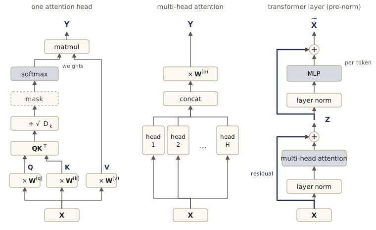
\[\mathbb{E}\left[\mathbf{q}^{\mathrm{T}}\mathbf{k}\right] = \sum_{i=1}^{D_k} \mathbb{E}[q_i]\,\mathbb{E}[k_i] = 0, \qquad \operatorname{var}\left[\mathbf{q}^{\mathrm{T}}\mathbf{k}\right] = \sum_{i=1}^{D_k} \mathbb{E}\left[q_i^2\right]\mathbb{E}\left[k_i^2\right] = D_k ,\]where the variances add because the terms \(q_i k_i\) are independent, each with mean zero and variance one. The scores therefore have standard deviation \(\sqrt{D_k}\), and dividing them by \(\sqrt{D_k}\) brings them back to unit variance whatever the key dimension. The result is scaled dot-product self-attention, and one copy of it, with its own three weight matrices, is called an attention head.
Result. Scaled dot-product attention is
\[\mathbf{Y} = \operatorname{Attention}(\mathbf{Q}, \mathbf{K}, \mathbf{V}) = \operatorname{Softmax}\left[\frac{\mathbf{Q}\mathbf{K}^{\mathrm{T}}}{\sqrt{D_k}}\right]\mathbf{V},\]with \(\mathbf{Q} = \mathbf{X}\mathbf{W}^{(q)}\), \(\mathbf{K} = \mathbf{X}\mathbf{W}^{(k)}\), and \(\mathbf{V} = \mathbf{X}\mathbf{W}^{(v)}\).
Here it is as a function. It takes an optional boolean mask that marks which query–key pairs are allowed; forbidden scores are set to \(-\infty\) before the softmax, so they get weight exactly zero and the remaining weights still sum to one. We will need the mask for language models and for padding. The function works on any leading batch dimensions, since @ and transpose(-2, -1) act on the last two.
def attention(Q, K, V, mask=None):
    """Scaled dot-product attention, Softmax(Q K^T / sqrt(D_k)) V.
    Q: (..., N, D_k), K: (..., M, D_k), V: (..., M, D_v).
    mask: boolean, broadcastable to (..., N, M); True = query n may attend to key m."""
    L = Q @ K.transpose(-2, -1) / math.sqrt(Q.shape[-1])
    if mask is not None:
        L = L.masked_fill(~mask, float("-inf"))
    A = torch.softmax(L, dim=-1)                      # each row sums to one
    return A @ V, A
Let us check the variance argument and see what saturation does. For random queries and keys with unit-variance elements, the variance of the raw dot product tracks \(D_k\), and the scaled one stays near 1:
g = torch.Generator().manual_seed(1)
for Dk in [4, 16, 64, 256]:
    q = torch.randn(20000, Dk, generator=g)
    k = torch.randn(20000, Dk, generator=g)
    s = (q * k).sum(dim=1)                            # 20000 dot products q^T k
    print(f"D_k = {Dk:3d}:  var(q^T k) = {s.var().item():7.2f}"
          f"   var(q^T k / sqrt(D_k)) = {(s / math.sqrt(Dk)).var().item():.3f}")
D_k =   4:  var(q^T k) =    4.03   var(q^T k / sqrt(D_k)) = 1.007
D_k =  16:  var(q^T k) =   16.36   var(q^T k / sqrt(D_k)) = 1.023
D_k =  64:  var(q^T k) =   64.58   var(q^T k / sqrt(D_k)) = 1.009
D_k = 256:  var(q^T k) =  259.84   var(q^T k / sqrt(D_k)) = 1.015
Now take one query and ten keys and compare the attention weights with and without scaling, along with the size of the softmax Jacobian, which is what gradients must pass through:
def softmax_jacobian_norm(l):
    a = torch.softmax(l, dim=-1)
    J = torch.diag(a) - torch.outer(a, a)             # d a_i / d l_j for a softmax
    return J.norm().item()

g = torch.Generator().manual_seed(2)
for Dk in [4, 64, 512]:
    q, Kx = torch.randn(Dk, generator=g), torch.randn(10, Dk, generator=g)
    for scale in [1.0, math.sqrt(Dk)]:
        l = Kx @ q / scale
        a_max = torch.softmax(l, -1).max()
        print(f"D_k = {Dk:3d}, divide by {scale:5.2f}:  largest weight {a_max:.3f}"
              f"   Jacobian norm {softmax_jacobian_norm(l):.2e}")
D_k =   4, divide by  1.00:  largest weight 0.311   Jacobian norm 3.75e-01
D_k =   4, divide by  2.00:  largest weight 0.202   Jacobian norm 3.26e-01
D_k =  64, divide by  1.00:  largest weight 0.995   Jacobian norm 9.60e-03
D_k =  64, divide by  8.00:  largest weight 0.410   Jacobian norm 3.64e-01
D_k = 512, divide by  1.00:  largest weight 1.000   Jacobian norm 9.17e-07
D_k = 512, divide by 22.63:  largest weight 0.424   Jacobian norm 3.66e-01
Without scaling, a 512-dimensional head puts essentially all its weight on one key and the Jacobian is almost zero, so almost no gradient reaches the queries and keys. With scaling the weights stay spread out and the Jacobian keeps the same size across dimensions.
Multi-head attention
One head produces one pattern of attention per token. Often several relations matter at once: in a sentence, one might link a verb to its subject while another tracks which words are in the same clause. A single head would have to average them. Multi-head attention runs \(H\) heads in parallel, each with its own projections,
\[\mathbf{H}_h = \operatorname{Attention}\left(\mathbf{X}\mathbf{W}^{(q)}_h, \mathbf{X}\mathbf{W}^{(k)}_h, \mathbf{X}\mathbf{W}^{(v)}_h\right), \qquad h = 1, \dots, H,\]concatenates their \(N \times D_v\) outputs side by side, and maps the result back to \(D\) features with an output matrix \(\mathbf{W}^{(o)}\) of size \(HD_v \times D\):
\[\mathbf{Y}(\mathbf{X}) = \operatorname{Concat}\left[\mathbf{H}_1, \dots, \mathbf{H}_H\right] \mathbf{W}^{(o)} .\]This is the attention analogue of having many filters in a convolutional layer. The usual choice is \(D_k = D_v = D/H\), so the concatenation is \(N \times D\) and the cost is about that of one full-width head. In code we do not loop over heads. We compute \(\mathbf{X}\mathbf{W}^{(q)}\) with one \(D \times D\) matrix whose column block \(h\) is \(\mathbf{W}^{(q)}_h\), reshape the result so that the heads become a batch dimension, and let attention handle all heads at once.
class MultiHeadAttention(nn.Module):
    """H heads of scaled dot-product attention, concatenated and projected by W^(o).
    Queries come from X; keys and values come from Z (Z = X gives self-attention)."""

    def __init__(self, D, H):
        super().__init__()
        assert D % H == 0
        self.H, self.Dh = H, D // H                       # D_k = D_v = D / H for each head
        s = 1 / math.sqrt(D)
        self.Wq = nn.Parameter(torch.randn(D, D) * s)     # [W_1^(q), ..., W_H^(q)] side by side
        self.Wk = nn.Parameter(torch.randn(D, D) * s)
        self.Wv = nn.Parameter(torch.randn(D, D) * s)
        self.Wo = nn.Parameter(torch.randn(D, D) * s)     # W^(o), size (H D_v) x D

    def split(self, M):
        """(B, N, D) -> (B, H, N, D/H): column block h of M goes to head h."""
        B, N, _ = M.shape
        return M.view(B, N, self.H, self.Dh).transpose(1, 2)

    def forward(self, X, Z=None, mask=None):
        Z = X if Z is None else Z
        Q, K, V = self.split(X @ self.Wq), self.split(Z @ self.Wk), self.split(Z @ self.Wv)
        Hs, self.A = attention(Q, K, V, mask)             # heads (B, H, N, D/H); weights kept
        B, H, N, Dh = Hs.shape
        concat = Hs.transpose(1, 2).reshape(B, N, H * Dh) # Concat[H_1, ..., H_H]
        return concat @ self.Wo
PyTorch’s nn.MultiheadAttention implements the same computation. It stores the three input projections stacked in one matrix and applies weights as \(\mathbf{x}\mathbf{W}^{\mathrm{T}}\), so we copy our matrices in transposed. If our layer is right, both outputs and the per-head attention weights must agree:
torch.manual_seed(0)
D, H, N = 16, 4, 7
mha = MultiHeadAttention(D, H)
X = torch.randn(2, N, D)                              # a batch of two sequences
Y = mha(X)

ref = nn.MultiheadAttention(D, H, bias=False, batch_first=True)
with torch.no_grad():
    ref.in_proj_weight.copy_(torch.cat([mha.Wq.T, mha.Wk.T, mha.Wv.T]))
    ref.out_proj.weight.copy_(mha.Wo.T)
Y_ref, A_ref = ref(X, X, X, need_weights=True, average_attn_weights=False)
print("output shape:", tuple(Y.shape))
print("outputs match nn.MultiheadAttention:", torch.allclose(Y, Y_ref, atol=1e-6))
print("attention weights match:            ", torch.allclose(mha.A, A_ref, atol=1e-6))
output shape: (2, 7, 16)
outputs match nn.MultiheadAttention: True
attention weights match:             True
The formulation has some redundancy: head \(h\)’s values are multiplied first by \(\mathbf{W}^{(v)}_h\) and then by the block \(\mathbf{W}^{(o)}_h\) of rows of \(\mathbf{W}^{(o)}\) that it meets in the concatenation. Writing \(\mathbf{A}_h\) for head \(h\)’s attention matrix, the layer is a sum over heads,
\[\mathbf{Y} = \sum_{h=1}^{H} \mathbf{A}_h \mathbf{X} \mathbf{W}^{(v)}_h \mathbf{W}^{(o)}_h ,\]where each product \(\mathbf{W}^{(v)}_h \mathbf{W}^{(o)}_h\) is a \(D \times D\) matrix of rank at most \(D/H\). Let us confirm it, and count parameters:
Wv_h = mha.Wv.view(D, H, D // H)                      # W_h^(v) = Wv_h[:, h]
Wo_h = mha.Wo.view(H, D // H, D)                      # W_h^(o) = Wo_h[h]
Y_sum = sum(mha.A[:, h] @ X @ (Wv_h[:, h] @ Wo_h[h]) for h in range(H))
print("sum-over-heads form matches:", torch.allclose(Y, Y_sum, atol=1e-5))
print("parameters:", sum(p.numel() for p in mha.parameters()), "= 4 D^2 =", 4 * D * D)
sum-over-heads form matches: True
parameters: 1024 = 4 D^2 = 1024
The parameter count, \(4D^2\), does not depend on the number of tokens \(N\) or the number of heads \(H\).
Transformer layers
To stack attention layers deeply, we borrow two tools from earlier modules. A residual connection (module 09) adds the layer’s input to its output, which requires the output to be \(N \times D\) like the input. Layer normalization (module 07) then standardizes each token’s \(D\) features to zero mean and unit variance, followed by a learned scale and shift. In the original arrangement, called post-norm, the normalization comes after the addition:
\[\mathbf{Z} = \operatorname{LayerNorm}\left[\mathbf{Y}(\mathbf{X}) + \mathbf{X}\right].\]Attention alone has a limited range of outputs. Each output is a weighted sum of value vectors, and the values are linear in the inputs, so every output row lies in the span of the input rows (at most \(N\) dimensions, and a linear image of it). The nonlinearity enters only through the weights. To transform features more freely, each layer adds an MLP, a small two-layer network with \(D\) inputs and \(D\) outputs (usually with a hidden layer of about \(4D\) units), applied to every token separately with shared weights so that any number of tokens can be processed. It gets its own residual connection and normalization:
\[\widetilde{\mathbf{X}} = \operatorname{LayerNorm}\left[\operatorname{MLP}[\mathbf{Z}] + \mathbf{Z}\right].\]Many current models use pre-norm instead, normalizing the input of each sub-layer and leaving the residual path untouched:
\[\begin{aligned} \mathbf{Z} &= \mathbf{Y}(\mathbf{X}') + \mathbf{X}, & \mathbf{X}' &= \operatorname{LayerNorm}[\mathbf{X}], \\ \widetilde{\mathbf{X}} &= \operatorname{MLP}[\mathbf{Z}'] + \mathbf{Z}, & \mathbf{Z}' &= \operatorname{LayerNorm}[\mathbf{Z}]. \end{aligned}\]In pre-norm, the input reaches the output of a stack of layers through a chain of additions only, which tends to make deep stacks easier to optimize; post-norm models are commonly trained with a learning-rate warmup (module 07). A stack uses the same structure in every layer, with separate parameters.
class TransformerLayer(nn.Module):
    """Multi-head self-attention and a position-wise MLP, each with a residual connection
    and layer normalization, in pre-norm (default) or post-norm arrangement."""

    def __init__(self, D, H, prenorm=True):
        super().__init__()
        self.prenorm = prenorm
        self.mha = MultiHeadAttention(D, H)
        self.ln1, self.ln2 = nn.LayerNorm(D), nn.LayerNorm(D)
        self.mlp = nn.Sequential(nn.Linear(D, 4 * D), nn.GELU(), nn.Linear(4 * D, D))

    def forward(self, X, mask=None):
        if self.prenorm:
            Z = X + self.mha(self.ln1(X), mask=mask)      # Z = Y(X') + X
            return Z + self.mlp(self.ln2(Z))              # X~ = MLP(Z') + Z
        Z = self.ln1(X + self.mha(X, mask=mask))          # Z = LayerNorm[Y(X) + X]
        return self.ln2(Z + self.mlp(Z))                  # X~ = LayerNorm[MLP(Z) + Z]
The hidden units use the GELU activation, \(\operatorname{GELU}(a) = a\,\Phi(a)\) with \(\Phi\) the standard normal distribution function, a smooth relative of the ReLU that is common in transformers. To see the two arrangements behave differently, push a random input through twelve freshly initialized layers of each kind and record the average length of the token vectors after each layer:
for prenorm in [False, True]:
    torch.manual_seed(3)
    stack = [TransformerLayer(32, 4, prenorm) for _ in range(12)]
    Z = torch.randn(8, 20, 32)
    norms = []
    with torch.no_grad():
        for layer in stack:
            Z = layer(Z)
            norms.append(Z.norm(dim=-1).mean().item())
    print("pre-norm " if prenorm else "post-norm", np.round(norms, 2))
post-norm [5.66 5.66 5.66 5.66 5.66 5.66 5.66 5.66 5.66 5.66 5.66 5.66]
pre-norm  [ 6.1   6.57  7.16  8.14  9.24  9.98 10.99 12.09 12.64 14.01 14.54 15.74]
Post-norm renormalizes after every layer, so each token has length close to \(\sqrt{32} \approx 5.66\) (layer norm makes the mean square of the features one). In pre-norm, each layer adds its contribution to a residual stream that is never renormalized, so the vectors grow steadily with depth. That is why pre-norm models apply one final layer norm before the output layer, as ours will.
Computational complexity
An attention layer maps \(ND\) numbers to \(ND\) numbers. A fully connected layer doing the same would need \((ND)^2\) weights and \(O(N^2D^2)\) operations, and it could only handle one sequence length. Attention shares its projections across tokens, so it has \(O(D^2)\) parameters. Its cost has two parts: computing \(\mathbf{Q}\), \(\mathbf{K}\), \(\mathbf{V}\) and the output projection takes \(O(ND^2)\), and forming \(\mathbf{Q}\mathbf{K}^{\mathrm{T}}\) and multiplying by \(\mathbf{V}\) takes \(O(N^2D)\). The MLP costs \(O(ND^2)\), linear in \(N\). So for short sequences the per-token matrix products dominate, and for long ones the \(N \times N\) attention matrix does, in both time and memory. One way to see an attention layer is as a large fully connected layer that is mostly zeros, with the nonzero blocks sharing parameters (exercise 3 asks you to draw it).
The timing below holds \(D = 64\) fixed and doubles \(N\). (Timings depend on your machine and its load; your times will differ, but the growth rates should not.)
torch.manual_seed(0)
Dt = 64
Wq_t, Wk_t, Wv_t = (torch.randn(Dt, Dt) for _ in range(3))
mlp_t = nn.Sequential(nn.Linear(Dt, 4 * Dt), nn.ReLU(), nn.Linear(4 * Dt, Dt))

def best_time(f, repeats=3):
    best = float("inf")
    for _ in range(repeats):
        t0 = time.perf_counter(); f(); best = min(best, time.perf_counter() - t0)
    return best

with torch.no_grad():
    for Nt in [256, 512, 1024, 2048, 4096]:
        Xt = torch.randn(Nt, Dt)
        t_att = best_time(lambda: attention(Xt @ Wq_t, Xt @ Wk_t, Xt @ Wv_t))
        t_mlp = best_time(lambda: mlp_t(Xt))
        print(f"N = {Nt:4d}:  attention {1e3 * t_att:7.1f} ms   MLP {1e3 * t_mlp:5.1f} ms")
N =  256:  attention     1.7 ms   MLP   0.2 ms
N =  512:  attention     5.6 ms   MLP   0.5 ms
N = 1024:  attention    18.8 ms   MLP   1.0 ms
N = 2048:  attention   101.5 ms   MLP   2.3 ms
N = 4096:  attention   354.7 ms   MLP   4.4 ms
Each doubling of \(N\) multiplies the attention time by roughly four and the MLP time by roughly two. Much research has gone into cheaper approximations of attention for long sequences; Bishop & Bishop §12.1.8 points to surveys.
Positional encoding
Nothing in a transformer layer refers to the position of a token. The projections and the MLP are shared across tokens, and attention treats its inputs as a set. So if we reorder the input rows with a permutation matrix \(\mathbf{P}\), the output rows are reordered in the same way: \(\operatorname{TransformerLayer}[\mathbf{P}\mathbf{X}] = \mathbf{P}\operatorname{TransformerLayer}[\mathbf{X}]\). The layer is permutation equivariant. The proof is short: \((\mathbf{P}\mathbf{X})\mathbf{W}\) permutes the rows of \(\mathbf{X}\mathbf{W}\); the scores become \(\mathbf{P}\mathbf{Q}\mathbf{K}^{\mathrm{T}}\mathbf{P}^{\mathrm{T}}\), whose row-wise softmax is \(\mathbf{P}\mathbf{A}\mathbf{P}^{\mathrm{T}}\); multiplying by \(\mathbf{P}\mathbf{V}\) gives \(\mathbf{P}\mathbf{A}\mathbf{V}\) since \(\mathbf{P}^{\mathrm{T}}\mathbf{P} = \mathbf{I}\); and residuals, layer norm, and the MLP act row by row.
torch.manual_seed(4)
layer = TransformerLayer(16, 4)
X = torch.randn(1, 7, 16)
perm = torch.randperm(7)
with torch.no_grad():
    Y_perm, Y = layer(X[:, perm]), layer(X)
print("layer(X[perm]) == layer(X)[perm]:", torch.allclose(Y_perm, Y[:, perm], atol=1e-5))
layer(X[perm]) == layer(X)[perm]: True
Equivariance is useful for sets, and it lets long-range and short-range interactions be learned equally easily. For sequences it is a problem. “The dog bit the man” and “The man bit the dog” contain the same tokens and would get the same set of outputs. We need to put order information into the tokens themselves, leaving the layer unchanged.
The usual approach gives each position \(n\) a positional encoding vector \(\mathbf{r}_n\) and adds it to the token embedding, \(\widetilde{\mathbf{x}}_n = \mathbf{x}_n + \mathbf{r}_n\). Concatenating would also work, but it enlarges every subsequent layer. Adding might seem to corrupt the token, but two things help: in high dimensions two unrelated vectors are nearly orthogonal (we check this below), so the network can still separate identity from position; and after a linear map, a concatenation \([\mathbf{x}; \mathbf{r}]\) becomes \(\mathbf{W}_1\mathbf{x} + \mathbf{W}_2\mathbf{r}\), which is again a sum. The residual connections carry the position information up through the layers.
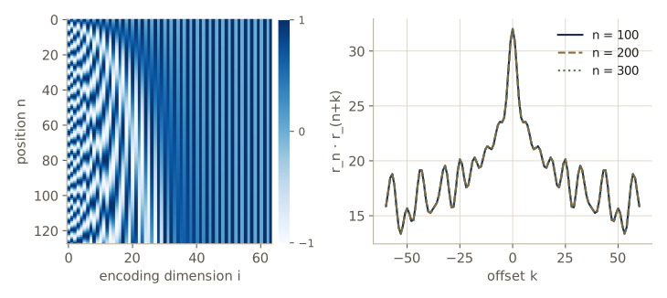
What makes a good encoding? It should be unique for each position, bounded, defined for positions longer than any seen in training, and it should make the offset between two positions easy to read off, since relative position often matters more than absolute position. The integer \(n\) itself is unbounded; \(n/N\) depends on the sequence length. The sinusoidal encoding of the original transformer paper uses sines and cosines at geometrically spaced frequencies. With \(D\) even and \(j = 0, \dots, D/2 - 1\),
\[r_{n, 2j} = \sin(\omega_j n), \qquad r_{n, 2j+1} = \cos(\omega_j n), \qquad \omega_j = L^{-2j/D},\]with \(L = 10000\) in the original paper. The first pair oscillates fastest; later pairs have ever longer wavelengths, much as the bits of a binary counter flip at rates that halve from one bit to the next, but with smooth values in \([-1, 1]\).
def sinusoidal_encoding(N, D, L=10000.0):
    """r_{n,2j} = sin(w_j n), r_{n,2j+1} = cos(w_j n), w_j = L^(-2j/D), positions n = 0..N-1."""
    n = torch.arange(N, dtype=torch.float64)[:, None]
    omega = L ** (-torch.arange(0, D, 2, dtype=torch.float64) / D)
    R = torch.zeros(N, D, dtype=torch.float64)
    R[:, 0::2] = torch.sin(n * omega)
    R[:, 1::2] = torch.cos(n * omega)
    return R, omega

R, omega = sinusoidal_encoding(2000, 32)
print("shape", tuple(R.shape), " range [%.3f, %.3f]" % (R.min().item(), R.max().item()))
wavelength = 2 * math.pi / omega
print("wavelengths 2 pi / w_j (first, last): %.1f, %.1f" % (wavelength[0], wavelength[-1]))
min_dist = torch.cdist(R, R).add(torch.eye(2000) * 1e9).min().item()    # closest pair n != m
print("all 2000 encodings distinct:", min_dist > 1e-3)
shape (2000, 32)  range [-1.000, 1.000]
wavelengths 2 pi / w_j (first, last): 6.3, 35332.9
all 2000 encodings distinct: True
The key property is about offsets. For a fixed shift \(k\), the addition formulas give, for each frequency,
\[\begin{pmatrix} \sin(\omega_j(n+k)) \\ \cos(\omega_j(n+k)) \end{pmatrix} = \begin{pmatrix} \cos\omega_j k & \sin\omega_j k \\ -\sin\omega_j k & \cos\omega_j k \end{pmatrix} \begin{pmatrix} \sin\omega_j n \\ \cos\omega_j n \end{pmatrix}.\]So \(\mathbf{r}_{n+k} = \mathbf{M}_k \mathbf{r}_n\), where \(\mathbf{M}_k\) is block diagonal with one \(2 \times 2\) rotation per frequency and depends on \(k\) but not on \(n\). A linear layer can therefore express “look \(k\) positions back” in the same way at every position. The same rotation structure makes the dot product \(\mathbf{r}_n^{\mathrm{T}}\mathbf{r}_m = \sum_j \cos(\omega_j (n - m))\) a function of the offset alone. The construction needs both sines and cosines: with sines only, there is no matrix that maps every \(\mathbf{r}_n\) to \(\mathbf{r}_{n+k}\), because \(\sin(\omega(n+k))\) is not determined by \(\sin(\omega n)\) alone.
def shift_matrix(omega, k):
    """Block-diagonal M_k with r_{n+k} = M_k r_n (one 2x2 rotation per frequency)."""
    Dm = 2 * len(omega)
    M = torch.zeros(Dm, Dm, dtype=torch.float64)
    c, s = torch.cos(omega * k), torch.sin(omega * k)
    for j in range(len(omega)):
        M[2 * j:2 * j + 2, 2 * j:2 * j + 2] = torch.stack([torch.stack([c[j], s[j]]),
                                                           torch.stack([-s[j], c[j]])])
    return M

k = 7
Mk = shift_matrix(omega, k)
err = (R[k:] - R[:-k] @ Mk.T).abs().max()                # rows: r_(n+k)^T = r_n^T M_k^T
print("max error of r_{n+7} = M_7 r_n over n = 0..1992: %.1e" % err)
G = R @ R.T
print("r_n . r_(n+3) at n = 10, 500, 1500: %.4f %.4f %.4f"
      % (G[10, 13], G[500, 503], G[1500, 1503]))

Rs = R[:, 0::2]                                        # sines only
M_ls = torch.linalg.lstsq(Rs[:-k], Rs[k:]).solution    # best single linear map, all n
res = (Rs[:-k] @ M_ls - Rs[k:]).pow(2).mean().sqrt()
print("sines only: RMS error of the best linear shift map %.3f" % res)
max error of r_{n+7} = M_7 r_n over n = 0..1992: 2.0e-13
r_n . r_(n+3) at n = 10, 500, 1500: 12.2724 12.2724 12.2724
sines only: RMS error of the best linear shift map 0.311
The map is exact to rounding error, the dot product of encodings three apart is the same at every position, and without cosines even the best linear map misses badly. The claim about near-orthogonality is also quick to check: the cosine of the angle between two random directions in \(D\) dimensions has mean zero and standard deviation \(1/\sqrt{D}\) (exercise 4).
for Dr in [4, 64, 1024]:
    a = rng.standard_normal((5000, Dr))
    b = rng.standard_normal((5000, Dr))
    cos = np.sum(a * b, 1) / (np.linalg.norm(a, axis=1) * np.linalg.norm(b, axis=1))
    print(f"D = {Dr:4d}: std of cos(angle) = {cos.std():.4f}   1/sqrt(D) = {1 / np.sqrt(Dr):.4f}")
D =    4: std of cos(angle) = 0.5012   1/sqrt(D) = 0.5000
D =   64: std of cos(angle) = 0.1281   1/sqrt(D) = 0.1250
D = 1024: std of cos(angle) = 0.0312   1/sqrt(D) = 0.0312
The alternative is a learned positional encoding: one free vector per position, trained with everything else. It needs no design, but it breaks the property that motivated sinusoids, since positions never seen in training have untrained vectors. It is a good choice when inputs have a fixed or bounded length, as in the language model and the vision transformer we train below.
Note. Positional information can also enter inside attention rather than in the input, for instance by adding a learned bias that depends on the offset \(n - m\) to the score \(\mathbf{q}_n^{\mathrm{T}}\mathbf{k}_m\), or by rotating queries and keys by position-dependent angles as in the shift matrices above. These relative schemes are popular in recent language models; the sinusoidal and learned absolute encodings covered here are the ones in Bishop & Bishop and remain a good starting point.
Natural language
Transformers were invented for language, and language is where most of their vocabulary comes from. English, like many languages, is a sequence of words separated by spaces and punctuation. Before a network can process it, we must decide what the tokens are and how each becomes a vector. We then need a model for sequences of tokens. This section covers the preparation and the models that came before transformers; the next puts transformers to work.
Word embedding
With a fixed dictionary of \(K\) words, the simplest numerical form of a word is one-hot: a \(K\)-dimensional vector with a single 1 at the word’s index. It is enormous for a realistic vocabulary (hundreds of thousands of entries) and it makes all words equally different from each other. A word embedding instead represents each word by a dense vector in a space of modest dimension \(D\) (a few hundred is typical). It is defined by a \(D \times K\) matrix \(\mathbf{E}\):
\[\mathbf{v}_n = \mathbf{E}\mathbf{x}_n ,\]and since \(\mathbf{x}_n\) is one-hot, \(\mathbf{v}_n\) is just the column of \(\mathbf{E}\) for that word. In code no multiplication happens at all: the embedding is a table lookup. PyTorch’s nn.Embedding stores \(\mathbf{E}^{\mathrm{T}}\), one row per word:
K_demo, D_demo = 10, 3
emb = nn.Embedding(K_demo, D_demo)                   # weight is E^T, shape (K, D)
E = emb.weight.detach().T                             # E, shape (D, K)
word = torch.tensor(7)
x = F.one_hot(word, K_demo).float()                   # one-hot x_n
print("E x      :", (E @ x).numpy())
print("column 7 :", E[:, 7].numpy())
print("lookup   :", emb(word).detach().numpy())
E x      : [ 0.9786  0.9664 -0.7578]
column 7 : [ 0.9786  0.9664 -0.7578]
lookup   : [ 0.9786  0.9664 -0.7578]
The matrix can be learned from unlabeled text. word2vec is a two-layer linear network trained on windows of a few consecutive words. In the continuous bag-of-words variant the network sees the words around a gap and predicts the word in the gap; in the skip-gram variant it sees the middle word and predicts each of its neighbors. The labels come from the text itself, so this is self-supervised learning, and after training the relevant weight matrix serves as \(\mathbf{E}\). Words that occur in similar contexts, such as “violin” and “cello”, need similar vectors to make similar predictions, so they land close together. The learned spaces also turned out to support some vector arithmetic: the offset from a country to its capital is roughly the same for many pairs, so \(\mathbf{v}(\text{Paris}) - \mathbf{v}(\text{France}) + \mathbf{v}(\text{Italy})\) lands near \(\mathbf{v}(\text{Rome})\).
Today embeddings are rarely a separate product. They are the first layer of a larger network, either initialized from a pre-trained table or, more often, learned end to end along with everything else, as ours will be.
Tokenization
Word-level dictionaries have gaps: new words, misspellings, names, numbers, and code are not in them, and punctuation needs special treatment. Going to the other extreme, characters, removes the gaps (a few dozen symbols cover English text) but makes sequences several times longer and forces the network to rediscover words from letters. Tokenization in current practice sits in between: a preprocessing step splits text into subword units that include frequent words whole, common fragments such as “ing” or “tion”, and single characters as a fallback. Related words then share pieces: “play”, “plays”, “played”, and “player” can all contain the token “play”.
Byte-pair encoding (BPE) builds such a vocabulary greedily. It starts from the individual characters and repeats one step: find the most frequent pair of adjacent tokens in a training text and add their concatenation as a new token, replacing every occurrence of the pair. To keep tokens from spanning two words, a pair is never merged if its second token starts with whitespace. The number of merges, and hence the vocabulary size, is fixed in advance as a compromise between characters and words.
We need a text to work with. Tiny Shakespeare is about a million characters of Shakespeare’s plays in one file:
os.makedirs("data", exist_ok=True)
path = "data/tinyshakespeare.txt"
if not os.path.exists(path):
    urllib.request.urlretrieve("https://raw.githubusercontent.com/karpathy/char-rnn/master/"
                               "data/tinyshakespeare/input.txt", path)
text = open(path).read()
print(f"{len(text):,} characters")
print(text[:120])
1,115,394 characters
First Citizen:
Before we proceed any further, hear me speak.

All:
Speak, speak.

First Citizen:
You are all resolved ra
Because merges never join a token to one that begins with whitespace, the text falls apart into independent chunks, each a whitespace character followed by the non-space characters after it (“ citizens,”, “\nFirst”). We can therefore count each distinct chunk once, with its frequency, instead of scanning the whole text at every step, which is the standard trick for training BPE quickly.
def merge_pair(tokens, a, b):
    """Replace every adjacent occurrence of (a, b) in a token list by the token a + b."""
    out, i = [], 0
    while i < len(tokens):
        if i + 1 < len(tokens) and tokens[i] == a and tokens[i + 1] == b:
            out.append(a + b)
            i += 2
        else:
            out.append(tokens[i])
            i += 1
    return out

def bpe_train(text, n_merges):
    """Learn n_merges BPE merges; a pair (a, b) is never merged when b starts with whitespace."""
    chunks = Counter(re.findall(r"\s?\S+|\s", text))          # whitespace + following word
    words = {tuple(w): f for w, f in chunks.items()}           # each chunk as a token tuple
    merges = []
    for _ in range(n_merges):
        pairs = Counter()
        for w, f in words.items():
            for a, b in zip(w, w[1:]):
                if not b[0].isspace():
                    pairs[a, b] += f
        (a, b), count = pairs.most_common(1)[0]
        merges.append((a, b))
        new_words = Counter()
        for w, f in words.items():
            new_words[tuple(merge_pair(list(w), a, b))] += f
        words = new_words
    return merges

def bpe_encode(s, merges):
    """Tokenize a string by applying the learned merges in the order they were learned."""
    tokens = list(s)
    for a, b in merges:
        tokens = merge_pair(tokens, a, b)
    return tokens

merges = bpe_train(text[:100_000], 200)
print("first 24 merges:", [a + b for a, b in merges[:24]])
print("last 12 merges: ", [a + b for a, b in merges[-12:]])
first 24 merges: [' t', 'he', 'ou', ' a', ' the', ' s', ' w', 're', 'ha', 'in', ' m', ' b', 'nd', 'it', 'on', 'er', ' y', 'or', 'll', 'es', 'is', 'en', ' c', ' f']
last 12 merges:  ['es,', '\nTo', '\nBR', '\nBRU', '\nBRUTUS:', ' hear', ' r', ' de', ' se', 'ak', '\nWe', ' con']
The first merges join a space to a common first letter (“ t”, “ a”) and build frequent pieces such as “he” and “ou”; “ the”, with its leading space, is a single token by the fifth merge, and among the last merges are pieces of a speaker’s name at the start of a line. Here is how the tokenizer splits a line of the play and a sentence it has never seen, and how many characters a token covers on average on held-out text as the merges accumulate:
print(bpe_encode("First Citizen: we are accounted poor citizens.", merges))
print(bpe_encode("The transformer tokenizes unfamiliar words.", merges))
held_out = text[-20_000:]
for m in [0, 50, 100, 200]:
    n_tok = len(bpe_encode(held_out, merges[:m]))
    print(f"{m:3d} merges: vocabulary {65 + m:3d},  "
          f"{len(held_out) / n_tok:.2f} characters per token")
['F', 'irst', ' C', 'itizen', ':', ' we', ' are', ' a', 'c', 'c', 'ou', 'n', 't', 'ed', ' p', 'o', 'or', ' c', 'itizen', 's', '.']
['T', 'he', ' t', 'r', 'an', 's', 'f', 'or', 'm', 'er', ' to', 'k', 'en', 'i', 'z', 'es', ' ', 'un', 'f', 'a', 'm', 'i', 'l', 'i', 'ar', ' wor', 'd', 's', '.']
  0 merges: vocabulary  65,  1.00 characters per token
 50 merges: vocabulary 115,  1.37 characters per token
100 merges: vocabulary 165,  1.57 characters per token
200 merges: vocabulary 265,  1.76 characters per token
Unfamiliar words fall back to smaller pieces instead of failing, and each merge makes sequences shorter. Production tokenizers work on bytes rather than characters (so any input, in any script, can be encoded) and learn tens of thousands of merges from far more text. For the rest of this module we use the 65 characters of Tiny Shakespeare as tokens, which keeps the models small and the outputs easy to read.
Bag of words
Now for models of token sequences, that is, of the joint distribution \(p(\mathbf{x}_1, \dots, \mathbf{x}_N)\). The crudest assumes every token is drawn independently from one shared distribution,
\[p(\mathbf{x}_1, \dots, \mathbf{x}_N) = \prod_{n=1}^{N} p(\mathbf{x}_n).\]As a graphical model (module 11) this has no edges at all. The distribution \(p(\mathbf{x})\) is a table with one probability per vocabulary entry, and maximizing the likelihood subject to the probabilities summing to one (a Lagrange multiplier, exercise 5) gives the relative frequencies in the training text. Word order plays no role, hence the name bag of words.
Bags of words still make useful classifiers. A naive Bayes classifier keeps one table per class \(\mathcal{C}_k\) and assumes the tokens are independent given the class, so that
\[p(\mathcal{C}_k \mid \mathbf{x}_1, \dots, \mathbf{x}_N) \propto p(\mathcal{C}_k) \prod_{n=1}^{N} p(\mathbf{x}_n \mid \mathcal{C}_k),\]with every factor estimated by counting. Classifying product reviews as positive or negative is the classic use. A word that never occurred with a class in training would make the whole product zero, so the counts are smoothed, for instance by adding a small pseudo-count to every entry.
We set up the character data once: the vocabulary, the text as a tensor of integer ids, a 90/10 split into training and validation text (the same split as module 11), a function that draws random windows, and a function that measures the average cross-entropy of any model on fixed validation windows. Every model below reports its loss through evaluate, so the numbers are comparable.
chars = sorted(set(text))
K = len(chars)                                        # vocabulary size
stoi = {c: i for i, c in enumerate(chars)}
decode = lambda ids: "".join(chars[i] for i in ids)
ids = torch.tensor([stoi[c] for c in text])
n_train = int(0.9 * len(ids))
train_ids, val_ids = ids[:n_train], ids[n_train:]
print(f"K = {K} characters; {len(train_ids):,} training and {len(val_ids):,} validation tokens")

def get_batch(data, B, N, g):
    """B random windows of N + 1 consecutive tokens: inputs x_1..x_N and targets x_2..x_(N+1)."""
    start = torch.randint(len(data) - N - 1, (B,), generator=g)
    x = torch.stack([data[s:s + N] for s in start])
    t = torch.stack([data[s + 1:s + N + 1] for s in start])
    return x, t

@torch.no_grad()
def evaluate(logits_fn, data=val_ids, n_batches=8, B=64, N=64):
    """Average next-token cross-entropy (nats per token) on the same fixed windows every time."""
    g = torch.Generator().manual_seed(123)
    losses = []
    for _ in range(n_batches):
        x, t = get_batch(data, B, N, g)
        losses.append(F.cross_entropy(logits_fn(x).reshape(-1, K), t.reshape(-1)).item())
    return float(np.mean(losses))

counts = torch.bincount(train_ids, minlength=K).double()
p_uni = (counts + 1) / (counts + 1).sum()             # relative frequencies, pseudo-count 1
loss_uni = evaluate(lambda x: torch.log(p_uni).float().expand(*x.shape, K))
print(f"unigram (bag of characters): {loss_uni:.4f} nats/char,"
      f" perplexity {math.exp(loss_uni):.2f}")
K = 65 characters; 1,003,854 training and 111,540 validation tokens
unigram (bag of characters): 3.3580 nats/char, perplexity 28.73
We report the average negative log likelihood per token in nats; module 11 used bits, which are nats divided by \(\ln 2\). The perplexity \(\exp(\text{loss})\) is the effective number of equally likely choices the model is left with at each step: knowing only letter frequencies, it is as unsure as if it were picking uniformly among about 29 characters.
Autoregressive models
To use word order, factorize the joint distribution by the product rule, exactly as in module 11:
\[p(\mathbf{x}_1, \dots, \mathbf{x}_N) = \prod_{n=1}^{N} p(\mathbf{x}_n \mid \mathbf{x}_1, \dots, \mathbf{x}_{n-1}).\]This is exact, and as a graphical model it links every token to all earlier ones. Storing each conditional as a table is hopeless, since a table conditioned on \(n - 1\) previous tokens has \(K^{n}\) entries. An n-gram model keeps only the last \(L\) tokens of context, \(p(\mathbf{x}_n \mid \mathbf{x}_{n-L}, \dots, \mathbf{x}_{n-1})\), with the same table at every position. \(L = 1\) gives a bigram model, \(L = 2\) a trigram model. The tables are estimated by counting and still grow like \(K^{L+1}\), so in practice \(L\) stays small, and samples from such models are locally plausible but lose the thread after a few tokens. Module 11 fitted character Markov chains of several orders to this text. We need just the bigram as a baseline:
C2 = torch.zeros(K, K, dtype=torch.float64)
C2.index_put_((train_ids[:-1], train_ids[1:]), torch.ones(n_train - 1, dtype=torch.float64),
              accumulate=True)                        # C2[a, b] = count of "a followed by b"
P2 = (C2 + 1) / (C2 + 1).sum(dim=1, keepdim=True)     # p(x_n = b | x_(n-1) = a)
log_P2 = torch.log(P2).float()
loss_bi = evaluate(lambda x: log_P2[x])               # the row of log p for each previous token
print(f"bigram: {loss_bi:.4f} nats/char, perplexity {math.exp(loss_bi):.2f}"
      f" ({loss_bi / math.log(2):.3f} bits/char)")

g = torch.Generator().manual_seed(5)
out = [stoi["\n"]]
for _ in range(150):                                  # ancestral sampling, one character at a time
    out.append(torch.multinomial(P2[out[-1]], 1, generator=g).item())
print(decode(out))
bigram: 2.4859 nats/char, perplexity 12.01 (3.586 bits/char)

WA h n, thea oble s I I lly mommay t ng
Whe te t strkimanthequriant od chalegepe bee y ee KIZWARDI k'tr RUKIUCorer.
OLourth wn ouplamawheaveathe llt s
One character of context cuts the perplexity by more than half. The sample has the texture of English, with short words, spaces, and capitalized speaker names, but no words. Another way to reach further back without exploding tables is a hidden Markov model, where the influence of the past must pass through a chain of latent states; recurrent networks are the neural version of that idea.
Recurrent neural networks
A feed-forward network has a fixed number of inputs, while sentences vary in length. And a word, or phrase, means much the same wherever it appears, which suggests sharing parameters across positions, as convolutions share them across an image. A recurrent neural network (RNN) does both by keeping a hidden state \(\mathbf{z}_n\) that is updated as each token arrives. At every step the same network takes the current input and the previous state and produces a new state and an output:
\[\mathbf{z}_n = \tanh\left(\mathbf{W}^{(zx)}\mathbf{x}_n + \mathbf{W}^{(zz)}\mathbf{z}_{n-1} + \mathbf{b}\right), \qquad \mathbf{y}_n = \operatorname{Softmax}\left(\mathbf{W}^{(yz)}\mathbf{z}_n + \mathbf{c}\right),\]starting from \(\mathbf{z}_0 = \mathbf{0}\). For a language model, \(\mathbf{y}_n\) is the predicted distribution of the next token, so the network is an autoregressive model whose context is summarized in \(\mathbf{z}_n\). The number of parameters does not depend on the sequence length. Since \(\mathbf{x}_n\) is one-hot, \(\mathbf{W}^{(zx)}\mathbf{x}_n\) is again an embedding lookup. Here is the network written out, one time step per loop iteration:
class RNN(nn.Module):
    """Elman RNN language model: z_n = tanh(W_zx x_n + W_zz z_(n-1) + b), logits = W_yz z_n + c."""

    def __init__(self, K, M):
        super().__init__()
        self.M = M
        self.W_zx = nn.Parameter(torch.randn(K, M) * 0.1)          # row x_n = W_zx x_n (lookup)
        self.W_zz = nn.Parameter(torch.randn(M, M) / math.sqrt(M))
        self.b = nn.Parameter(torch.zeros(M))
        self.W_yz = nn.Parameter(torch.randn(M, K) / math.sqrt(M))
        self.c = nn.Parameter(torch.zeros(K))

    def forward(self, x, z=None):
        B, N = x.shape
        z = torch.zeros(B, self.M) if z is None else z
        states = []
        for n in range(N):                                         # strictly sequential
            z = torch.tanh(self.W_zx[x[:, n]] + z @ self.W_zz + self.b)
            states.append(z)
        Zs = torch.stack(states, dim=1)                            # (B, N, M)
        return Zs @ self.W_yz + self.c                             # logits for every position
We train it with Adam on random 64-character windows. The loss is the cross-entropy summed over all positions of each window (averaged, in practice), so every character is a training target for the prefix before it. We clip the gradient norm at 1, for reasons the next subsection makes clear. The time in brackets is the wall-clock time on our CPU; your times will differ, here and in the other training cells.
torch.manual_seed(12)
rnn = RNN(K, 128)
opt = torch.optim.Adam(rnn.parameters(), lr=3e-3)
g = torch.Generator().manual_seed(1)
t0 = time.time()
for step in range(301):
    x, t = get_batch(train_ids, 32, 64, g)
    loss = F.cross_entropy(rnn(x).reshape(-1, K), t.reshape(-1))
    opt.zero_grad()
    loss.backward()
    torch.nn.utils.clip_grad_norm_(rnn.parameters(), 1.0)
    opt.step()
    if step % 100 == 0:
        print(f"step {step:3d}  training loss {loss.item():.3f}")
loss_rnn = evaluate(lambda x: rnn(x))
print(f"RNN ({sum(p.numel() for p in rnn.parameters()):,} parameters): validation {loss_rnn:.4f}"
      f" nats/char, perplexity {math.exp(loss_rnn):.2f}   [{time.time() - t0:.0f} s]")
step   0  training loss 4.211
step 100  training loss 2.487
step 200  training loss 2.223
step 300  training loss 2.160
RNN (33,217 parameters): validation 2.1878 nats/char, perplexity 8.92   [7 s]
After a few hundred steps the RNN is already well below the bigram. RNNs were also the standard tool for translation. An encoder–decoder RNN reads the whole source sentence, then a special start token, and from then on emits the translation one word at a time, feeding each emitted word back in as the next input until it produces a stop token. The outputs during the reading phase are ignored. Everything the decoder knows about the source must pass through the single state vector at the moment reading ends. For long sentences that fixed-size vector is a bottleneck, and relieving it was the original motivation for attention, which lets the decoder look back at every encoder state directly.
Backpropagation through time
An RNN unrolled over \(N\) steps is a deep feed-forward network with shared weights, one layer per time step, so its gradients come from ordinary backpropagation through the unrolled graph (module 08). This is called backpropagation through time. It is simple in principle. The difficulty is depth. Write \(\mathbf{a}_m\) for the argument of tanh at step \(m\), so \(\mathbf{z}_m = \tanh(\mathbf{a}_m)\). The chain rule through the recurrence gives
\[\frac{\partial \mathbf{z}_m}{\partial \mathbf{z}_{m-1}} = \operatorname{diag}\left(1 - \mathbf{z}_m^2\right)\mathbf{W}^{(zz)}, \qquad \frac{\partial E}{\partial \mathbf{z}_n} = \left(\prod_{m=n+1}^{N} \frac{\partial \mathbf{z}_m}{\partial \mathbf{z}_{m-1}}\right)^{\mathrm{T}} \frac{\partial E}{\partial \mathbf{z}_N}\]for an error \(E\) that depends on the last state (the product is ordered with later steps on the left). Since \(0 < 1 - z^2 \leq 1\), each factor has norm at most the largest singular value \(s_{\max}\) of \(\mathbf{W}^{(zz)}\), so
\[\left\lVert \frac{\partial E}{\partial \mathbf{z}_n} \right\rVert \leq s_{\max}^{\,N-n} \left\lVert \frac{\partial E}{\partial \mathbf{z}_N} \right\rVert .\]If \(s_{\max} < 1\) the signal from step \(N\) decays exponentially on its way back: vanishing gradients, which means the network cannot learn how its early inputs affect later errors. If the recurrent weights are large and the units are not saturated, the product can instead grow exponentially: exploding gradients, which make training steps erratic. We can watch both happen. We build recurrent matrices \(g\mathbf{Q}\) from a random orthogonal \(\mathbf{Q}\), so that every singular value equals the gain \(g\), run 60 steps on random inputs, and backpropagate a random linear function of the final state:
def bptt_gradient_norms(gain, M=64, N=60, seed=0):
    """||dE/dz_n|| for n = 1..N in a tanh RNN with W_zz = gain * (random orthogonal matrix)."""
    gen = torch.Generator().manual_seed(seed)
    Qo, _ = torch.linalg.qr(torch.randn(M, M, generator=gen))
    W_zz = gain * Qo
    x = 0.5 * torch.randn(N, M, generator=gen)       # inputs already multiplied by W_zx
    z = torch.zeros(M, requires_grad=True)
    states = []
    for n in range(N):
        z = torch.tanh(x[n] + z @ W_zz)
        z.retain_grad()                              # keep dE/dz_n for inspection
        states.append(z)
    E = states[-1] @ torch.randn(M, generator=gen)    # a random linear error of the last state
    E.backward()
    return np.array([s.grad.norm().item() for s in states])

for gain in [0.5, 1.0, 1.5, 3.0]:
    gn = bptt_gradient_norms(gain)
    print(f"gain {gain:3.1f}:  ||dE/dz_n|| at n = N, N-10, N-30, N-59: "
          + "  ".join(f"{gn[i]:9.2e}" for i in [59, 49, 29, 0]))
gain 0.5:  ||dE/dz_n|| at n = N, N-10, N-30, N-59:  9.08e+00   1.20e-03   2.38e-11   1.50e-22
gain 1.0:  ||dE/dz_n|| at n = N, N-10, N-30, N-59:  9.08e+00   5.06e-01   1.47e-03   4.18e-07
gain 1.5:  ||dE/dz_n|| at n = N, N-10, N-30, N-59:  9.08e+00   7.46e+00   2.42e+00   1.31e+00
gain 3.0:  ||dE/dz_n|| at n = N, N-10, N-30, N-59:  9.08e+00   7.77e+01   5.36e+03   2.24e+06
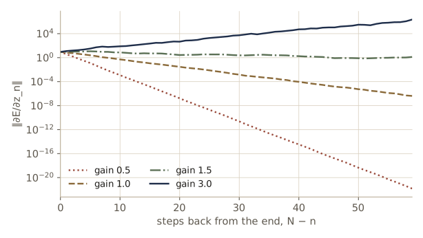
With gain 0.5 the gradient reaching the first step is more than twenty orders of magnitude smaller than at the last step. Even gain 1 vanishes, by about seven orders of magnitude over 60 steps, because the tanh derivatives are below one. Gain 3 explodes, growing by a factor of about \(10^5\). Only a narrow band in between keeps the gradient roughly level, and training does not stay in such a band by itself. Gradient clipping, which rescales the gradient whenever its norm exceeds a threshold, handles explosion cheaply; we used it above.
Vanishing gradients need an architectural fix: a path along which information can travel many steps without being repeatedly squashed. The long short-term memory (LSTM) cell keeps a separate cell state that is updated additively, \(\mathbf{c}_n = \mathbf{f}_n \odot \mathbf{c}_{n-1} + \mathbf{i}_n \odot \mathbf{g}_n\), where the forget gate \(\mathbf{f}_n\) and input gate \(\mathbf{i}_n\) are sigmoid functions of the input and the previous state and \(\mathbf{g}_n\) is a tanh candidate update. When the forget gate is near one, the gradient flows back through \(\mathbf{c}\) almost unchanged, much as it flows through a residual connection. The gated recurrent unit (GRU) is a simpler cell built on the same idea. Both work far better than the plain RNN, but they do not remove the deeper limitations: every path from an early token to a late one still passes through all the steps in between, a long passage must fit in one fixed-size state, and the loop over time cannot be parallelized within a sequence, which wastes the parallel hardware that modern training relies on. Transformers remove all three: every token is one attention step from every other, and all positions are computed at once.
Transformer language models
Transformer language models fall into three families according to what goes in and what comes out. An encoder reads a sequence and produces a representation used for a fixed-size output, such as the sentiment of a review. A decoder generates a sequence, possibly conditioned on something else, such as a caption for an image. A sequence-to-sequence model does both, reading one sequence and writing another, as in translation. We build a small model of each kind, starting with the decoder, which is the basis of today’s large language models.
Decoder transformers
A decoder transformer is an autoregressive model in which every conditional \(p(\mathbf{x}_n \mid \mathbf{x}_1, \dots, \mathbf{x}_{n-1})\) is computed by one transformer. The best-known family is GPT (generative pre-trained transformer). The architecture is a stack of transformer layers on top of token embeddings plus positional encodings. At the top, each output token \(\widetilde{\mathbf{x}}_n\) (\(D\) numbers) is mapped to a distribution over the \(K\) vocabulary entries by a linear layer \(\mathbf{W}^{(p)}\) of size \(D \times K\), shared across positions, and a softmax:
\[\mathbf{Y} = \operatorname{Softmax}\left[\widetilde{\mathbf{X}}\mathbf{W}^{(p)}\right],\]with a cross-entropy error on each row. Generation works as for any autoregressive model: feed in a prefix, sample the next token from the last row of \(\mathbf{Y}\), append it, and repeat.
Training is where the transformer shines. A sequence of \(N + 1\) tokens contains \(N\) training examples: predict token 2 from token 1, token 3 from tokens 1 and 2, and so on. We would like to compute all \(N\) predictions in a single forward pass. Two changes make that possible. First, the targets are the inputs shifted by one place: output \(n\) is trained to predict token \(n + 1\). (Bishop & Bishop describe the equivalent arrangement in which a special start token is prepended to the input; our random windows already provide a first token to condition on.) Second, output \(n\) must not see tokens after \(n\), otherwise it could copy the answer, and at generation time those tokens do not exist yet. The only place tokens interact is attention, so we use masked attention (also called causal attention): attention weights from position \(n\) to any later position \(m > n\) are forced to zero, and each row is renormalized over the allowed positions. Setting the corresponding scores to \(-\infty\) before the softmax does both at once, which is what our attention function does with a lower-triangular mask.
def causal_mask(N):
    """True where query position n may attend to key position m, i.e. m <= n."""
    return torch.tril(torch.ones(N, N, dtype=torch.bool))

print(causal_mask(6).int().numpy())

torch.manual_seed(0)
layer = TransformerLayer(16, 4)
X1 = torch.randn(1, 10, 16)
X2 = X1.clone()
X2[:, 6:] = torch.randn(1, 4, 16)                     # change tokens 6..9 only
with torch.no_grad():
    Y1, Y2 = layer(X1, causal_mask(10)), layer(X2, causal_mask(10))
print("outputs 0..5 unchanged:", torch.allclose(Y1[:, :6], Y2[:, :6]))
print("outputs 6..9 unchanged:", torch.allclose(Y1[:, 6:], Y2[:, 6:]))
[[1 0 0 0 0 0]
 [1 1 0 0 0 0]
 [1 1 1 0 0 0]
 [1 1 1 1 0 0]
 [1 1 1 1 1 0]
 [1 1 1 1 1 1]]
outputs 0..5 unchanged: True
outputs 6..9 unchanged: False
With the causal mask, changing the last four tokens leaves the first six outputs exactly as they were. The same property makes generation cheaper than it looks. When a new token is appended, the representations of all earlier tokens stay the same, so their keys and values can be stored and reused; only the new position needs computing. This key–value cache is how deployed models generate text.
Watch out. A decoder trained without the causal mask, or with targets that are not shifted by one, reaches a nearly perfect training loss, because each position can read the very token it is supposed to predict. Nothing crashes; the model is simply useless for generation. In a language model, a training loss that looks too good to be true is usually a masking or shifting bug.
Batches of real text contain sequences of different lengths. They are brought to a common length by appending a special padding token, and a second mask stops every position from attending to padding. Unlike the causal mask, this one depends on the input. With it, a padded sequence gives the same outputs at its real positions as the unpadded sequence would. We check this in a layer without a causal mask, where padding would otherwise leak into every position:
torch.manual_seed(1)
layer = TransformerLayer(16, 4)
real = torch.randn(1, 3, 16)                           # a sequence of length 3
padded = torch.cat([real, torch.zeros(1, 2, 16)], 1)   # padded to length 5
key_ok = torch.tensor([True, True, True, False, False])
with torch.no_grad():
    Y_alone = layer(real)
    Y_masked = layer(padded, mask=key_ok[None, :])     # every query may attend to real keys only
    Y_unmasked = layer(padded)
print("with padding mask, real positions match:   ",
      torch.allclose(Y_alone, Y_masked[:, :3], atol=1e-6))
print("without padding mask, real positions match:",
      torch.allclose(Y_alone, Y_unmasked[:, :3], atol=1e-6))
with padding mask, real positions match:    True
without padding mask, real positions match: False
Now the model itself. Following GPT, we use a learned positional encoding (inputs never exceed 64 characters here), pre-norm layers, and a final layer norm before the output projection. The softmax is left to F.cross_entropy, which takes logits.
class GPT(nn.Module):
    """Decoder-only transformer language model: embeddings + learned positions,
    L masked (causal) pre-norm transformer layers, final layer norm, linear output W^(p)."""

    def __init__(self, K, D=64, H=4, L=2, N_max=64):
        super().__init__()
        self.N_max = N_max
        self.tok = nn.Embedding(K, D)                              # token embedding
        self.pos = nn.Parameter(0.02 * torch.randn(N_max, D))      # learned positional encoding
        self.layers = nn.ModuleList([TransformerLayer(D, H) for _ in range(L)])
        self.ln = nn.LayerNorm(D)
        self.W_p = nn.Linear(D, K)                                 # output projection W^(p)
        self.register_buffer("mask", causal_mask(N_max))

    def forward(self, x):
        B, N = x.shape
        X = self.tok(x) + self.pos[:N]                             # x~_n = x_n + r_n
        for layer in self.layers:
            X = layer(X, mask=self.mask[:N, :N])
        return self.W_p(self.ln(X))                                # logits, (B, N, K)

torch.manual_seed(12)
gpt = GPT(K)
print(f"{sum(p.numel() for p in gpt.parameters()):,} parameters")
print(f"initial validation loss {evaluate(gpt):.4f} (uniform guessing: ln K = {math.log(K):.4f})")
112,065 parameters
initial validation loss 4.3794 (uniform guessing: ln K = 4.1744)
We train with AdamW, a linear warmup over the first 100 steps followed by cosine decay (the schedules of module 07), mini-batches of 32 windows of 64 characters, and 900 steps in total. Each window supplies 64 targets at once. The training is split over four cells so that each stays short; train_gpt keeps the step count and the loss history in state.
def lr_at(step, total=900, warmup=100, eta0=6e-3):
    """Linear warmup to eta0, then cosine decay to zero."""
    if step < warmup:
        return eta0 * (step + 1) / warmup
    return 0.5 * eta0 * (1 + math.cos(math.pi * (step - warmup) / (total - warmup)))

def train_gpt(model, opt, n_steps, state, g, report_every=150):
    t0 = time.time()
    for _ in range(n_steps):
        for group in opt.param_groups:
            group["lr"] = lr_at(state["step"])
        x, t = get_batch(train_ids, 32, 64, g)
        loss = F.cross_entropy(model(x).reshape(-1, K), t.reshape(-1))
        opt.zero_grad()
        loss.backward()
        opt.step()
        state["losses"].append(loss.item())
        state["step"] += 1
        if state["step"] % report_every == 0:
            print(f"step {state['step']:3d}  training loss (last 50 steps) "
                  f"{np.mean(state['losses'][-50:]):.3f}   validation {evaluate(model):.3f}")
    print(f"[{time.time() - t0:.0f} s]")

opt = torch.optim.AdamW(gpt.parameters(), lr=6e-3, weight_decay=0.01)
state = {"step": 0, "losses": []}
g_train = torch.Generator().manual_seed(0)
train_gpt(gpt, opt, 225, state, g_train)
step 150  training loss (last 50 steps) 2.450   validation 2.457
[13 s]
train_gpt(gpt, opt, 225, state, g_train)
step 300  training loss (last 50 steps) 2.328   validation 2.377
step 450  training loss (last 50 steps) 2.049   validation 2.110
[13 s]
train_gpt(gpt, opt, 225, state, g_train)
step 600  training loss (last 50 steps) 1.885   validation 1.990
[13 s]
train_gpt(gpt, opt, 225, state, g_train)
loss_gpt = evaluate(gpt)
for name, loss in [("unigram", loss_uni), ("bigram", loss_bi), ("RNN (300 steps)", loss_rnn),
                   ("GPT (900 steps)", loss_gpt)]:
    print(f"{name:16s} {loss:.4f} nats/char   perplexity {math.exp(loss):5.2f}")
step 750  training loss (last 50 steps) 1.786   validation 1.927
step 900  training loss (last 50 steps) 1.760   validation 1.909
[14 s]
unigram          3.3580 nats/char   perplexity 28.73
bigram           2.4859 nats/char   perplexity 12.01
RNN (300 steps)  2.1878 nats/char   perplexity  8.92
GPT (900 steps)  1.9085 nats/char   perplexity  6.74
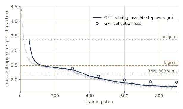
In under a minute of CPU time the transformer reaches a perplexity well below the bigram’s. Two cautions about the comparison with the RNN. After 300 steps the RNN was actually ahead (compare its loss with the GPT’s validation loss at step 300, early in the GPT’s schedule); both models are tiny and trained briefly, so the ranking says little about what either architecture can reach. And per step, our RNN was the cheaper model on this CPU. The transformer’s real advantages appear at scale: every position is trained in parallel, and any token can influence any later one in a single attention step. A larger model (say \(D = 384\), six layers, a context of 256 characters) trained on a GPU for a few thousand steps reaches a considerably lower loss on this data, and its samples read much more like the plays.
Here is a sample from the trained model, drawn one character at a time from its predicted distribution:
@torch.no_grad()
def generate(model, prompt, n_new, pick, g=None):
    """Extend prompt by n_new tokens; pick(logits, g) chooses the next token id."""
    x = torch.tensor([[stoi[c] for c in prompt]])
    for _ in range(n_new):
        logits = model(x[:, -model.N_max:])[0, -1]    # distribution for the next token
        x = torch.cat([x, torch.tensor([[pick(logits, g)]])], dim=1)
    return decode(x[0].tolist())

def sample_plain(logits, g):
    return torch.multinomial(torch.softmax(logits, -1), 1, generator=g).item()

print(generate(gpt, "ROMEO:\n", 300, sample_plain, torch.Generator().manual_seed(3)))
ROMEO:
Then neabter'd I thas beatte orst Rimes, you.

CLARIF ROUTK:
What, hellaf this now.
t he If welivese a is treppirent
And Rencemp cose, itr, to itw-feters and?
We my, hatht, poool me'st not hound that
that to dove, qhat nas lickse butlerts;
Harthough! he him stoorde, Eroven,
For mutielest our theeld
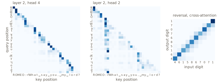
The model has learned the format of a play (speaker names in capitals followed by a colon, line breaks, short lines of verse), many common words, and some punctuation habits. It has not learned meaning; with 64 characters of context and a hundred thousand parameters, it could not. The attention weights show what the heads do. The figure below plots two heads of the second layer on one input line. Every row is confined to the lower triangle by the causal mask, and the two heads divide the work: one looks almost only at the current character and the one or two before it, while the other reaches further back, for instance to the previous space or the start of the line. (We picked the heads with the shortest and the longest average look-back distance in that layer.)
Sampling strategies
A trained decoder gives a distribution for the next token; we still have to choose a token. The choice matters a great deal in practice.
Greedy search takes the most probable token at every step. It is deterministic, and it does not find the most probable sequence. The probability of a whole sequence is the product of its conditionals,
\[p(\mathbf{y}_1, \dots, \mathbf{y}_N) = \prod_{n=1}^{N} p(\mathbf{y}_n \mid \mathbf{y}_1, \dots, \mathbf{y}_{n-1}),\]and a high-probability first token can lead to a spread-out distribution over what follows. A two-step example with tokens a and b shows it:
p_first = {"a": 0.6, "b": 0.4}
p_second = {"a": {"a": 0.5, "b": 0.5},                  # after a: both continuations equally likely
            "b": {"a": 0.9, "b": 0.1}}                  # after b: the next token is nearly certain
joint = {y1 + y2: p_first[y1] * p_second[y1][y2] for y1 in "ab" for y2 in "ab"}
y1 = max(p_first, key=p_first.get)
greedy_seq = y1 + max(p_second[y1], key=p_second[y1].get)
best_seq = max(joint, key=joint.get)
print("joint:", {s: round(p, 2) for s, p in joint.items()})
print(f"greedy picks {greedy_seq} with p = {joint[greedy_seq]:.2f}; the best sequence is"
      f" {best_seq} with p = {joint[best_seq]:.2f}")
joint: {'aa': 0.3, 'ab': 0.3, 'ba': 0.36, 'bb': 0.04}
greedy picks aa with p = 0.30; the best sequence is ba with p = 0.36
Finding the best sequence exactly would mean scoring all \(K^N\) sequences, while greedy search costs \(O(KN)\). Beam search sits in between. It keeps the \(B\) best partial sequences (the beam, of width \(B\)); at each step it extends each of them by its \(B\) most probable next tokens, scores the \(B^2\) candidates by their total log probability, and keeps the best \(B\). The cost is \(O(BKN)\), \(B\) times that of greedy search. When candidates can end at different lengths (with a stop token), longer sequences are penalized simply for having more factors below one, so scores are usually normalized by length before comparing; in our fixed-length runs that does not arise.
@torch.no_grad()
def beam_search(model, prompt, n_new, B=5):
    """Keep the B partial sequences with the highest total log probability."""
    beams = [(0.0, [stoi[c] for c in prompt])]
    for _ in range(n_new):
        x = torch.tensor([seq[-model.N_max:] for _, seq in beams])
        logp = F.log_softmax(model(x)[:, -1], dim=-1)            # (beams, K)
        candidates = []
        for (score, seq), lp in zip(beams, logp):
            top = lp.topk(B)
            for v, i in zip(top.values, top.indices):
                candidates.append((score + v.item(), seq + [i.item()]))
        beams = sorted(candidates, key=lambda c: c[0], reverse=True)[:B]
    return decode(beams[0][1])

@torch.no_grad()
def log_prob_per_char(model, prompt, continuation):
    """Average log p of the continuation's characters given everything before them."""
    x = torch.tensor([[stoi[c] for c in prompt + continuation]])[:, -model.N_max - 1:]
    logp = F.log_softmax(model(x[:, :-1])[0], dim=-1)
    tgt = x[0, 1:]
    return logp[torch.arange(len(tgt)), tgt][-len(continuation):].mean().item()

prompt = "KING RICHARD III:\n"
out_greedy = generate(gpt, prompt, 40, lambda l, g: l.argmax().item())
out_beam = beam_search(gpt, prompt, 40, B=5)
for name, s in [("greedy", out_greedy), ("beam, B = 5", out_beam)]:
    print(f"{name:12s} {log_prob_per_char(gpt, prompt, s[len(prompt):]):6.3f} nats/char  "
          f"{s[len(prompt):]!r}")
greedy       -0.968 nats/char  'I will the shall the shall the sond the '
beam, B = 5  -0.930 nats/char  'I will that the have that the have that '
Beam search finds a continuation with a higher average log probability than greedy search, as it should. Both outputs are dull and repetitive, and this is typical: the most probable continuations of text are bland, and maximizing probability tends to fall into loops. Human-written text is far less probable under a model than the model’s own most likely output. We can see that directly by scoring a genuine continuation from the validation text:
start = 2000
human = decode(val_ids[start:start + 60].tolist())
prompt_h, cont_h = human[:20], human[20:]
beam_h = beam_search(gpt, prompt_h, len(cont_h), B=5)[len(prompt_h):]
print(f"human continuation: {log_prob_per_char(gpt, prompt_h, cont_h):6.3f} nats/char  {cont_h!r}")
print(f"beam search:        {log_prob_per_char(gpt, prompt_h, beam_h):6.3f} nats/char  {beam_h!r}")
human continuation: -2.181 nats/char  'PTISTA:\nA thousand thanks, Signior Gremi'
beam search:        -0.824 nats/char  'LURENCE:\nWhat that with with that to the'
So instead of searching for the most probable text, we sample. Plain sampling from the softmax (what we did above) has the opposite problem: with a large vocabulary, the many individually unlikely tokens together hold a noticeable share of the probability, so every so often a nonsensical token is drawn, and later tokens are conditioned on it. Three controls trade quality against diversity:
- Top-k sampling keeps only the \(k\) most probable tokens, renormalizes, and samples from them.
- Nucleus or top-p sampling keeps the smallest set of most probable tokens whose total probability reaches \(p\), so the number of candidates adapts to how confident the model is.
- Temperature divides the logits by \(T\) before the softmax, \(y_i = \exp(a_i/T) / \sum_j \exp(a_j/T)\). As \(T \to 0\) this becomes greedy selection; \(T = 1\) is the model’s distribution; as \(T \to \infty\) it approaches the uniform distribution. Values below one sharpen the distribution toward its most likely tokens.
def sample(logits, g, T=1.0, top_k=None, top_p=None):
    """Sample a token from Softmax(logits / T), optionally restricted to the top k tokens
    or to the smallest set of top tokens with total probability >= top_p."""
    logits = logits / T
    if top_k is not None:
        kth = logits.topk(top_k).values[-1]
        logits = logits.masked_fill(logits < kth, float("-inf"))
    if top_p is not None:
        probs, order = torch.softmax(logits, -1).sort(descending=True)
        before = probs.cumsum(0) - probs                  # mass of the tokens ranked above each one
        drop = order[before >= top_p]                     # already reached p without them
        logits = logits.clone()
        logits[drop] = float("-inf")
    return torch.multinomial(torch.softmax(logits, -1), 1, generator=g).item()

context = "ROMEO:\nI will not s"
with torch.no_grad():
    logits_c = gpt(torch.tensor([[stoi[c] for c in context]]))[0, -1]
for T in [0.5, 1.0, 2.0]:
    p = torch.softmax(logits_c / T, -1)
    top = p.topk(3)
    print(f"T = {T}: entropy {-(p * p.log()).sum():.3f} nats; top 3:",
          ", ".join(f"{chars[i]!r} {v:.2f}" for v, i in zip(top.values, top.indices)))
p = torch.softmax(logits_c, -1).sort(descending=True).values
print("tokens needed to cover 90% of the probability (top-p = 0.9):",
      int((p.cumsum(0) < 0.9).sum()) + 1)
T = 0.5: entropy 1.816 nats; top 3: 'h' 0.31, 'o' 0.24, 't' 0.20
T = 1.0: entropy 2.279 nats; top 3: 'h' 0.20, 'o' 0.17, 't' 0.16
T = 2.0: entropy 2.936 nats; top 3: 'h' 0.12, 'o' 0.11, 't' 0.11
tokens needed to cover 90% of the probability (top-p = 0.9): 9
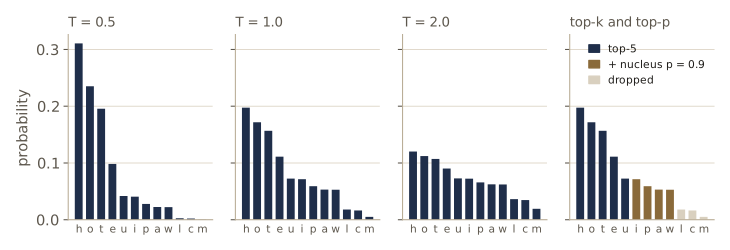
g = torch.Generator().manual_seed(7)
for name, kw in [("T = 0.5", dict(T=0.5)), ("top-k = 5", dict(top_k=5)),
                 ("top-p = 0.9", dict(top_p=0.9)), ("T = 1.5", dict(T=1.5))]:
    s = generate(gpt, "ROMEO:\n", 120, lambda l, g: sample(l, g, **kw), g)
    print(f"--- {name} ---\n{s[7:]}")
--- T = 0.5 ---
A do and scome of thy hear all sue,
The make and my that the bearr and of they are what charde the bear
and the strain h
--- top-k = 5 ---
Who thich than the toly trant ongute trus onest. That he she
And sires that tweend, and at marrrdon
To hum and sham as i
--- top-p = 0.9 ---
All the from no withined;
Whild neners, down wongely held are far was of
If that is that too the combe tows of news
more
--- T = 1.5 ---
S peYour; no, traiisteges, any errel ou'd what, conwat!
Pry aCfia&ord'
Mer:
Why gror undel, I seet la wiss
Forthoy tolln
Low temperature gives cleaner spelling and more repetition; high temperature gives more variety and more invented words. There is no single right setting, and deployed systems tune these controls per application.
One more issue belongs here. During training the model always conditions on real text, but during generation it conditions on its own output, which may drift away from anything seen in training; errors can then compound. This mismatch between training and use is inherent to training on next-token prediction and is one reason sampling controls matter.
Encoder transformers
An encoder transformer has the same stack of layers without the causal mask, so every output can attend to every input. It is not a generator. Its job is to produce representations of the input tokens for downstream tasks. The standard example is BERT (bidirectional encoder representations from transformers). A special class token is placed at the start of every input; its output is unused during pre-training and becomes the summary of the whole sequence during fine-tuning.
Without the causal mask, next-token prediction would be trivial, so encoders are pre-trained with a different self-supervised objective, the masked language model. A random subset of positions, typically 15%, is selected. The model sees the sequence with those positions corrupted and must predict the original tokens there; the loss counts only the selected positions. The word bidirectional refers to the fact that the prediction can use context on both sides. To reduce the mismatch with fine-tuning data, which never contains the mask symbol, the selected positions are corrupted in three ways: 80% are replaced by the mask token, 10% by a random token, and 10% are left unchanged (but must still be predicted). Here is that procedure, with the mask token shown as _:
MASK = K                                              # one extra token id for the mask symbol

def mask_tokens(x, g, p_select=0.15):
    """BERT-style corruption. Returns inputs and targets; unselected targets are -100 (ignored)."""
    select = torch.rand(x.shape, generator=g) < p_select
    u = torch.rand(x.shape, generator=g)
    x_in = x.clone()
    x_in[select & (u < 0.8)] = MASK                                  # 80%: mask token
    swap = select & (u >= 0.8) & (u < 0.9)                           # 10%: random token
    x_in[swap] = torch.randint(K, x.shape, generator=g)[swap]
    targets = torch.where(select, x, torch.full_like(x, -100))       # 10%: unchanged
    return x_in, targets

g = torch.Generator().manual_seed(4)
line = ids[:60][None, :]
x_in, tgt = mask_tokens(line, g)
show = lambda s: "".join("_" if i == MASK else chars[i] for i in s.tolist())
print(repr(show(line[0])))
print(repr(show(x_in[0])))
print("positions to predict:", (tgt[0] != -100).nonzero().flatten().tolist())

x_big, _ = get_batch(train_ids, 256, 64, g)
x_in, tgt = mask_tokens(x_big, g)
sel = tgt != -100
frac_masked = (x_in[sel] == MASK).float().mean()
frac_same = (x_in[sel] == x_big[sel]).float().mean()
print(f"selected {sel.float().mean():.3f};  of these: masked {frac_masked:.3f},"
      f" unchanged {frac_same:.3f}")
'First Citizen:\nBefore we proceed any further, hear me speak.'
'Fi_s_ Citizen:\nBefo_e we proceed any further, hear me__peak.'
positions to predict: [2, 4, 5, 19, 53, 54]
selected 0.151;  of these: masked 0.789, unchanged 0.110
The unchanged share comes out slightly above 10% because a random replacement occasionally draws the original token. The loss is F.cross_entropy(logits, targets, ignore_index=-100), so only about 15% of the positions provide a training signal, compared with all of them in a decoder. That is one reason encoders learn less per token processed. The same recipe, applied to image patches, gives the masked autoencoders of module 19.
After pre-training, the encoder is fine-tuned for a task with a small labeled data set. For classifying a whole text into \(K\) classes, a new \(D \times K\) linear layer and softmax (or a \(D \times 1\) layer and a logistic sigmoid for two classes) is attached to the class token’s output. For labeling each token (is this word a person, a place, a date?), a shared linear-softmax layer is attached to every other output. All parameters, old and new, are then trained on the task’s labels by gradient descent on the log likelihood.
Sequence-to-sequence transformers
The original transformer was an encoder–decoder model for translation. The encoder turns the source sentence into a matrix of representations \(\mathbf{Z}\), one row per source token. The decoder is a decoder transformer as above, generating the target sentence one token at a time, but each of its layers has an extra sub-layer that looks at \(\mathbf{Z}\). That sub-layer is cross-attention: attention in which the queries come from the sequence being generated and the keys and values come from the encoder output,
\[\mathbf{Y} = \operatorname{Softmax}\left[\frac{(\mathbf{X}\mathbf{W}^{(q)})(\mathbf{Z}\mathbf{W}^{(k)})^{\mathrm{T}}}{\sqrt{D_k}}\right]\mathbf{Z}\mathbf{W}^{(v)} .\]The attention matrix is now \(N_{\text{target}} \times N_{\text{source}}\), and no causal mask is needed there, because the whole source is known. In the library picture, the reader takes their request to a different library and gets books from its shelves. A decoder layer is thus masked self-attention, cross-attention, and an MLP, each with a residual connection and layer norm. Our MultiHeadAttention already accepts a separate Z for keys and values, so cross-attention needs no new code.
class DecoderLayer(nn.Module):
    """Pre-norm decoder layer: masked self-attention, cross-attention to encoder output Z, MLP."""

    def __init__(self, D, H):
        super().__init__()
        self.self_att, self.cross_att = MultiHeadAttention(D, H), MultiHeadAttention(D, H)
        self.ln1, self.ln2, self.ln3 = nn.LayerNorm(D), nn.LayerNorm(D), nn.LayerNorm(D)
        self.mlp = nn.Sequential(nn.Linear(D, 4 * D), nn.GELU(), nn.Linear(4 * D, D))

    def forward(self, X, Z, mask):
        X = X + self.self_att(self.ln1(X), mask=mask)
        X = X + self.cross_att(self.ln2(X), Z=Z)          # queries from X, keys and values from Z
        return X + self.mlp(self.ln3(X))

class Seq2Seq(nn.Module):
    def __init__(self, V, N, D=32, H=2):
        super().__init__()
        self.emb = nn.Embedding(V + 1, D)                 # V symbols plus a start token
        self.pos_src = nn.Parameter(0.1 * torch.randn(N, D))
        self.pos_tgt = nn.Parameter(0.1 * torch.randn(N, D))
        self.encoder = TransformerLayer(D, H)
        self.decoder = DecoderLayer(D, H)
        self.ln, self.out = nn.LayerNorm(D), nn.Linear(D, V)

    def forward(self, src, tgt_in):
        Z = self.encoder(self.emb(src) + self.pos_src)                # no mask: sees all of src
        X = self.emb(tgt_in) + self.pos_tgt[:tgt_in.shape[1]]
        X = self.decoder(X, Z, causal_mask(tgt_in.shape[1]))
        return self.out(self.ln(X))
A real translation task needs far more data and compute than we have, so we use a task where cross-attention has an obvious right answer: reverse a string of ten random digits. The decoder input is the start token followed by the target shifted by one, as in the GPT.
V, N_digits, START = 10, 10, 10
torch.manual_seed(5)
s2s = Seq2Seq(V, N_digits)
opt = torch.optim.Adam(s2s.parameters(), lr=3e-3)
g = torch.Generator().manual_seed(5)
for step in range(301):
    src = torch.randint(0, V, (64, N_digits), generator=g)
    tgt = src.flip(1)                                              # target: the reversed string
    tgt_in = torch.cat([torch.full((64, 1), START), tgt[:, :-1]], dim=1)
    loss = F.cross_entropy(s2s(src, tgt_in).reshape(-1, V), tgt.reshape(-1))
    opt.zero_grad(); loss.backward(); opt.step()
    if step % 100 == 0:
        print(f"step {step:3d}  loss {loss.item():.4f}")

with torch.no_grad():                                              # greedy decoding of new strings
    src = torch.randint(0, V, (500, N_digits), generator=g)
    out = torch.full((500, 1), START)
    for n in range(N_digits):
        out = torch.cat([out, s2s(src, out)[:, -1].argmax(-1, keepdim=True)], dim=1)
    print(f"strings reversed exactly: {(out[:, 1:] == src.flip(1)).all(1).float().mean():.3f}")
    A_cross = s2s.decoder.cross_att.A[0].mean(0)                   # first string, mean over heads
print("cross-attention (rows: output position, columns: input position):")
print(A_cross.numpy().round(2))
step   0  loss 2.5365
step 100  loss 0.9875
step 200  loss 0.0164
step 300  loss 0.0098
strings reversed exactly: 0.990
cross-attention (rows: output position, columns: input position):
[[0.   0.   0.   0.   0.   0.   0.   0.   0.01 0.99]
 [0.   0.   0.   0.   0.   0.   0.   0.11 0.6  0.29]
 [0.   0.   0.   0.   0.   0.01 0.03 0.79 0.14 0.03]
 [0.   0.   0.   0.   0.01 0.24 0.48 0.22 0.05 0.  ]
 [0.   0.   0.   0.   0.1  0.7  0.12 0.08 0.   0.  ]
 [0.   0.   0.   0.11 0.67 0.16 0.04 0.   0.   0.  ]
 [0.02 0.01 0.14 0.55 0.22 0.07 0.   0.   0.   0.  ]
 [0.01 0.07 0.57 0.29 0.06 0.   0.   0.   0.   0.  ]
 [0.12 0.8  0.07 0.01 0.   0.   0.   0.   0.   0.  ]
 [0.71 0.13 0.09 0.04 0.02 0.   0.   0.   0.   0.  ]]
The weight in each row of the cross-attention matrix sits on or next to the anti-diagonal: to write output position \(n\), the decoder looks mainly at input position \(9 - n\). Nobody told it to; the alignment was learned from the loss alone. In translation, cross-attention learns the analogous soft alignment between words of the two languages. Seen from a distance, attention passes messages between tokens along the edges of a fully connected graph, with learned edge weights; module 13 develops that view for general graphs.
Large language models
The most consequential development of recent years has been scaling decoder transformers up into large language models (LLMs), with billions of parameters or more, trained on a large fraction of the text available online together with code. Three things made this possible. The transformer maps efficiently onto large clusters of GPUs and similar processors, because all positions of a sequence are processed in parallel. Training is self-supervised, so every token of raw text is a labeled example and the data are no longer limited by human labeling. And performance has kept improving, fairly predictably, as model size, data, and compute grow together; much of the progress between successive generations of such models has come from scale rather than from changes in architecture.
Earlier language systems were trained by supervised learning on curated pairs, such as aligned sentences in two languages, and leaned on hand-designed features and constraints to compensate for small data. Self-supervised pre-training changed the recipe: train one large model on unlabeled text, then adapt it. A model with broad abilities that can be adapted to many tasks is called a foundation model, and the adaptation is a form of transfer learning. Fine-tuning continues training on a smaller labeled data set, updating all the weights, or only new output layers, or only a few of the existing weights.
Low-rank adaptation (LoRA) is an efficient way to fine-tune. It rests on the observation that the change in the weights needed to adapt a large pre-trained model tends to have low intrinsic dimension. LoRA freezes each chosen weight matrix \(\mathbf{W}_0\) (typically attention matrices, \(D \times D\)) and learns a low-rank correction:
\[\mathbf{X}\mathbf{W}_0 + \mathbf{X}\mathbf{A}\mathbf{B}, \qquad \mathbf{A} \in \mathbb{R}^{D \times R}, \; \mathbf{B} \in \mathbb{R}^{R \times D}, \; R \ll D .\]Only \(2RD\) numbers per matrix are trained instead of \(D^2\). \(\mathbf{B}\) starts at zero, so fine-tuning starts from the pre-trained model. After training, \(\widehat{\mathbf{W}} = \mathbf{W}_0 + \mathbf{A}\mathbf{B}\) is computed once, and inference costs exactly what it did before. For our small GPT:
R = 4
lora = {}
for i, layer in enumerate(gpt.layers):
    for name in ["Wq", "Wv"]:                                      # adapt queries and values
        W0 = getattr(layer.mha, name)
        A_l = nn.Parameter(0.01 * torch.randn(W0.shape[0], R))
        B_l = nn.Parameter(torch.zeros(R, W0.shape[1]))            # B = 0: start at the base model
        lora[f"layer{i}.{name}"] = (W0, A_l, B_l)
n_lora = sum(A_l.numel() + B_l.numel() for _, A_l, B_l in lora.values())
n_all = sum(p.numel() for p in gpt.parameters())
print(f"LoRA trains {n_lora:,} numbers instead of {n_all:,} ({100 * n_lora / n_all:.1f}%)")

W0, A_l, B_l = lora["layer0.Wq"]
with torch.no_grad():
    B_l.normal_()                                                  # pretend training changed B
    Xq = torch.randn(5, W0.shape[0])
    merged = Xq @ (W0 + A_l @ B_l)                                 # one matrix at inference
    separate = Xq @ W0 + Xq @ A_l @ B_l                            # frozen path + adapter path
    print("X W0 + X A B == X (W0 + A B):", torch.allclose(separate, merged, atol=1e-5))
LoRA trains 2,048 numbers instead of 112,065 (1.8%)
X W0 + X A B == X (W0 + A B): True
As models grew, fine-tuning became less necessary for many tasks, because a large model can be steered by its input alone. The input text is the prompt. To translate, you can give the model “English: the cat is asleep. French:” and let it continue; nothing in training targeted translation, but multilingual text in the training data makes the continuation a translation. A task can also be described by including a few worked examples in the prompt, which is called few-shot learning (no weights change). Designing prompts that produce good outputs has become a craft of its own, sometimes called prompt engineering, and systems commonly prepend fixed instructions to every user prompt.
A model pre-trained only to continue text is not yet a helpful assistant. Two further stages are common. Instruction tuning (supervised fine-tuning) continues training on examples of instructions or conversations paired with good responses, written or selected by people. Reinforcement learning from human feedback (RLHF) then collects human judgments of which of several model responses is better, trains a reward model to predict those preferences, and fine-tunes the language model to produce responses the reward model scores highly, while staying close to the original model so that it does not drift into degenerate text. These stages are what turn a text predictor into a conversational system that follows instructions. They are an active research area, and Bishop & Bishop §12.3.5 gives references.
In practice. Everything in our small GPT carries over to large models: embeddings, learned or relative positions, pre-norm layers with causal attention, a final layer norm, next-token cross-entropy, warmup with decay, and top-p or temperature sampling. What changes is scale (wider and deeper stacks, contexts of thousands of tokens or more, subword vocabularies of tens of thousands), engineering (mixed precision, distributing the model over many devices, key–value caching, memory-efficient attention kernels), and the post-training stages above.
Multimodal transformers
Transformers were designed to replace recurrent networks for text, but the same layer now leads in images, video, audio, point clouds, and combinations of these, for both recognition and generation. The reason is how little it assumes. A convolutional network assumes locality and translation equivariance; a transformer assumes only that its input is a set of tokens, plus whatever position information we add. The layer itself has changed little across applications. The work lies in turning each kind of data into tokens and turning output tokens back into data. Once that is done, combining kinds of data (multimodal models) is almost free: tokens from different sources can be placed in one sequence.
Vision transformers
For classification, the standard design is a transformer encoder applied to image patches, the vision transformer (ViT). Using every pixel as a token would make \(N\) huge, and attention costs \(O(N^2)\) in time and memory. Instead the image, of size \(H \times W\) with \(C\) channels, is cut into non-overlapping \(P \times P\) patches (16 × 16 is a common choice for photographs), and each patch is flattened into a vector of length \(P^2C\). That gives \(N = HW/P^2\) tokens per image, each mapped to \(D\) dimensions by a shared linear layer, the patch embedding. A learnable class token is prepended, learned positional encodings are added (explicit two-dimensional encodings exist but have not generally helped), and after the encoder a linear layer and softmax on the class token’s output give the class probabilities. Since all images have the same size, the number of tokens is fixed and learned positions pose no problem. An alternative tokenizer runs the image through a small CNN and uses its down-sampled feature map as the tokens.
For MNIST, 7 × 7 patches turn a 28 × 28 digit into a 4 × 4 grid of 16 tokens with 49 pixels each. Patchifying is a reshape and a permutation:
train = datasets.MNIST(root="data", train=True, download=True)
test = datasets.MNIST(root="data", train=False, download=True)
X_tr, y_tr = train.data[:6000].float().div(255.), train.targets[:6000]
X_te, y_te = test.data[:2000].float().div(255.), test.targets[:2000]

def patchify(X, P):
    """(B, H, W) images -> (B, HW/P^2, P^2): flattened P x P patches in raster order."""
    B, Hi, Wi = X.shape
    return X.view(B, Hi // P, P, Wi // P, P).permute(0, 1, 3, 2, 4).reshape(B, -1, P * P)

def unpatchify(T, P, Hi, Wi):
    B = T.shape[0]
    return T.view(B, Hi // P, Wi // P, P, P).permute(0, 1, 3, 2, 4).reshape(B, Hi, Wi)

T = patchify(X_tr[:2], 7)
print("tokens per image and features per token:", tuple(T.shape[1:]))
print("patch (1, 2) equals the image block rows 7-13, columns 14-20:",
      torch.equal(T[0, 1 * 4 + 2], X_tr[0, 7:14, 14:21].reshape(-1)))
print("unpatchify inverts patchify:", torch.equal(unpatchify(T, 7, 28, 28), X_tr[:2]))
tokens per image and features per token: (16, 49)
patch (1, 2) equals the image block rows 7-13, columns 14-20: True
unpatchify inverts patchify: True
The model reuses our TransformerLayer without a mask:
class ViT(nn.Module):
    """Vision transformer: patch embedding, class token, learned positions, encoder, linear head."""

    def __init__(self, P=7, D=48, H=4, L=2, n_classes=10, image_size=28):
        super().__init__()
        self.P = P
        n_patches = (image_size // P) ** 2
        self.embed = nn.Linear(P * P, D)                            # patch embedding
        self.cls = nn.Parameter(torch.zeros(1, 1, D))               # learnable class token
        self.pos = nn.Parameter(0.02 * torch.randn(1, n_patches + 1, D))
        self.layers = nn.ModuleList([TransformerLayer(D, H) for _ in range(L)])
        self.ln = nn.LayerNorm(D)
        self.head = nn.Linear(D, n_classes)

    def forward(self, X):
        T = self.embed(patchify(X, self.P))
        T = torch.cat([self.cls.expand(len(T), -1, -1), T], dim=1) + self.pos
        for layer in self.layers:
            T = layer(T)
        return self.head(self.ln(T[:, 0]))                          # read out the class token

torch.manual_seed(7)
vit = ViT()
opt = torch.optim.AdamW(vit.parameters(), lr=2e-3)
g = torch.Generator().manual_seed(7)
t0 = time.time()
for epoch in range(4):
    perm = torch.randperm(len(X_tr), generator=g)
    for i in range(0, len(X_tr), 64):
        b = perm[i:i + 64]
        loss = F.cross_entropy(vit(X_tr[b]), y_tr[b])
        opt.zero_grad(); loss.backward(); opt.step()
    with torch.no_grad():
        acc = (vit(X_te).argmax(1) == y_te).float().mean().item()
    print(f"epoch {epoch + 1}: test accuracy {acc:.3f}")
print(f"{sum(p.numel() for p in vit.parameters()):,} parameters  [{time.time() - t0:.0f} s]")
epoch 1: test accuracy 0.717
epoch 2: test accuracy 0.808
epoch 3: test accuracy 0.824
epoch 4: test accuracy 0.875
60,010 parameters  [9 s]
A tiny ViT with 16 tokens reaches 87.5% test accuracy in about ten seconds of training, but it falls short of what the small convolutional network of module 10 reaches on similar data. That is expected. A CNN has locality and translation equivariance built in; the only two-dimensional structure a ViT gets for free is the patch grid, and everything else, including which patches are neighbors, must be learned from data. With little data the built-in assumptions win. With very large data sets, fewer assumptions let transformers reach higher accuracy, one more instance of the balance between built-in assumptions and the amount of data. Longer training, data augmentation, and the full 60,000 images would improve our numbers considerably.
Generative image transformers
Can a transformer also generate images, as it generates text? Pixels have no natural order, but the product rule does not need one: after fixing any ordering, a joint distribution factorizes as \(p(\mathbf{x}_1, \dots, \mathbf{x}_N) = \prod_n p(\mathbf{x}_n \mid \mathbf{x}_1, \dots, \mathbf{x}_{n-1})\) (module 11). For images the usual choice is the raster scan, row by row from the top left, the order our patchify uses for patches. Sampling then paints the image one pixel (or patch) at a time. Autoregressive image models predate transformers: PixelRNN and PixelCNN computed the conditionals with recurrent layers and with convolutions masked so that each pixel sees only earlier ones.
How should a pixel be represented? A continuous conditional such as a Gaussian, trained by maximum likelihood, predicts an average, and averages of plausible images are blurry: where a pixel could be black or white, a Gaussian predicts gray. A discrete distribution over pixel values can put probability on both black and white instead. But an RGB pixel with 8 bits per channel has \(2^{24} \approx 1.7 \times 10^7\) values, far too many for a softmax, and a patch is hopeless (even binary 16 × 16 patches have \(2^{256}\) values). Vector quantization solves this. Choose a codebook of \(K\) vectors \(\mathbf{c}_1, \dots, \mathbf{c}_K\) and replace every data vector with the closest codebook vector,
\[\mathbf{x}_n \rightarrow \arg\min_{\mathbf{c}_k} \lVert \mathbf{x}_n - \mathbf{c}_k \rVert^2 ,\]so that each pixel or patch becomes an index in \(\{1, \dots, K\}\), a discrete token like a word. \(K\) trades accuracy for compression. The codebook can come from K-means clustering (module 15), which is how ImageGPT tokenized pixel colors. Here is K-means on the 4 × 4 patches of a thousand digits:
def kmeans(Xk, n_codes, n_iter, g):
    """Plain K-means (Lloyd's algorithm); returns the codebook and each row's code index."""
    C = Xk[torch.randperm(len(Xk), generator=g)[:n_codes]].clone()
    for _ in range(n_iter):
        idx = torch.cdist(Xk, C).argmin(dim=1)                    # nearest codebook vector
        for k in range(n_codes):
            members = Xk[idx == k]
            if len(members):
                C[k] = members.mean(dim=0)
    return C, torch.cdist(Xk, C).argmin(dim=1)

patches = patchify(X_tr[:1000], 4).reshape(-1, 16)                # 49 patches per image
g = torch.Generator().manual_seed(0)
for n_codes in [8, 32, 128]:
    C, idx = kmeans(patches, n_codes, 15, g)
    rel_err = ((patches - C[idx]) ** 2).sum() / (patches ** 2).sum()
    print(f"K = {n_codes:3d}: relative squared reconstruction error {rel_err:.3f};"
          f" an image becomes 49 tokens from a vocabulary of {n_codes}")
K =   8: relative squared reconstruction error 0.224; an image becomes 49 tokens from a vocabulary of 8
K =  32: relative squared reconstruction error 0.139; an image becomes 49 tokens from a vocabulary of 32
K = 128: relative squared reconstruction error 0.082; an image becomes 49 tokens from a vocabulary of 128
With 128 codes, each digit becomes 49 tokens and is reconstructed with under a tenth of its energy lost; an autoregressive transformer can then be trained on these token sequences exactly like a language model, and its samples decoded by looking up the codebook. Better codebooks are learned jointly with an encoder and decoder network (the VQ-VAE family, and variants that use transformers as the encoder), which raises a difficulty: \(\arg\min\) has zero gradient almost everywhere. The standard workaround is the straight-through estimator, which uses the quantized value in the forward pass but pretends quantization was the identity in the backward pass. In code it is one line:
z = torch.tensor([[0.3, 0.8], [0.9, 0.1]], requires_grad=True)   # encoder outputs
codebook = torch.tensor([[0.0, 1.0], [1.0, 0.0]])
q = codebook[torch.cdist(z, codebook).argmin(dim=1)]             # nearest codes
z_q = z + (q - z).detach()                                       # value q, gradient of identity
upstream = torch.tensor([[1.0, 2.0], [3.0, 4.0]])
(z_q * upstream).sum().backward()
print("forward value:", z_q.detach().numpy().tolist())
print("gradient reaching z:", z.grad.numpy().tolist())
forward value: [[0.0, 1.0], [1.0, 0.0]]
gradient reaching z: [[1.0, 2.0], [3.0, 4.0]]
The forward value is the code; the gradient that reaches the encoder output is exactly the upstream gradient. Video can be handled the same way, as one long sequence of vector-quantized tokens.
Audio data
Sound is recorded as a waveform, the air pressure sampled at regular intervals (thousands of times per second). Models rarely consume raw waveforms. The usual input is a spectrogram: cut the signal into short overlapping frames, multiply each by a smooth window, and take the magnitude of its discrete Fourier transform. The result is a matrix with one column per time frame and one row per frequency. A mel spectrogram then pools the frequencies into bands that are equally spaced on the mel scale, \(m = 2595 \log_{10}(1 + f/700)\), which approximates how people perceive pitch: bands are narrow at low frequencies and wide at high ones. We compute one for a synthetic signal, a tone sweeping upward from 300 Hz to 2000 Hz over one second with a steady 1000 Hz tone added halfway through, and check our spectrogram against torch.stft:
sr = 8000                                                         # samples per second
t = torch.arange(sr, dtype=torch.float64) / sr                    # one second
f_sweep = 300 + 1700 * t                                          # instantaneous frequency
sweep = torch.sin(2 * math.pi * (300 * t + 850 * t ** 2))    # phase' / 2 pi = f_sweep
tone = 0.5 * torch.sin(2 * math.pi * 1000 * t) * (t >= 0.5)          # 1000 Hz from t = 0.5 s on
wave = sweep + tone

n_fft, hop = 256, 128
window = torch.hann_window(n_fft, periodic=True, dtype=torch.float64)
frames = wave.unfold(0, n_fft, hop) * window                      # (frames, n_fft)
S = torch.fft.rfft(frames, dim=1).abs()                           # magnitude spectrogram (T, F)
S_ref = torch.stft(wave, n_fft, hop, window=window, center=False, return_complex=True).abs().T
freqs = torch.fft.rfftfreq(n_fft, 1 / sr, dtype=torch.float64)
print("spectrogram:", tuple(S.shape), " matches torch.stft:", torch.allclose(S, S_ref))
for fr in [5, 25, 45]:
    print(f"frame {fr}: strongest frequency {freqs[S[fr].argmax()]:6.1f} Hz,"
          f" sweep is at {f_sweep[fr * hop + n_fft // 2]:6.1f} Hz")
spectrogram: (61, 129)  matches torch.stft: True
frame 5: strongest frequency  468.8 Hz, sweep is at  463.2 Hz
frame 25: strongest frequency 1000.0 Hz, sweep is at 1007.2 Hz
frame 45: strongest frequency 1562.5 Hz, sweep is at 1551.2 Hz
The strongest frequency in each frame follows the sweep to within one frequency bin (31.25 Hz here). The mel filter bank is a set of triangular weights over the frequency bins, one triangle per band, with corners equally spaced on the mel scale:
mel = lambda f: 2595 * torch.log10(1 + f / 700)
mel_inv = lambda m: 700 * (10 ** (m / 2595) - 1)
n_mels = 32
m_top = mel(torch.tensor(sr / 2)).item()
edges = mel_inv(torch.linspace(0, m_top, n_mels + 2, dtype=torch.float64))   # equal steps in mel
rows = []
for lo, c, hi in zip(edges[:-2], edges[1:-1], edges[2:]):                    # a triangle per band
    rows.append(torch.clamp(torch.minimum((freqs - lo) / (c - lo), (hi - freqs) / (hi - c)), min=0))
fbank = torch.stack(rows)                                                     # (n_mels, F)
log_mel = torch.log(S ** 2 @ fbank.T + 1e-6)                                  # (T, n_mels)
print("log-mel spectrogram:", tuple(log_mel.shape))
print("band widths in Hz, lowest and highest band: %.0f, %.0f"
      % (edges[2] - edges[0], edges[-1] - edges[-3]))
n_tok = (log_mel.shape[0] // 8) * (log_mel.shape[1] // 8)
print("8 x 8 patches of the log-mel image:", n_tok, "tokens")
log-mel spectrogram: (61, 32)
band widths in Hz, lowest and highest band: 86, 512
8 x 8 patches of the log-mel image: 28 tokens
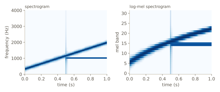
For audio classification (assigning a clip to categories such as “dog bark” or “engine”), the mel spectrogram used to be treated as an image and fed to a CNN. A CNN is good at local patterns but weaker at relating distant parts of a clip. Treating the spectrogram exactly like an image for a ViT, cutting it into patches (possibly overlapping), embedding them, adding positions and a class token, and training an encoder transformer with cross-entropy, now works better on standard benchmarks. The architecture is the same encoder we use for text and images; only the tokenizer changed.
Text-to-speech
Text-to-speech synthesis produces speech for a given text. The traditional approach trains a regression model to map text, or units of sound called phonemes, to spectrogram frames for one speaker, then converts the spectrogram to a waveform. It has three weaknesses. Predicting small units sounds choppy unless much context is used, while predicting large units needs enormous data. Nothing transfers from one speaker to another. And speech is not a function of text: there are many good ways to read a sentence, and regression averages them.
Treating speech as a language removes all three. A learned audio codec with a vector-quantized codebook turns speech into a sequence of discrete tokens, and a decoder transformer is trained as a conditional language model: the input is the text’s tokens followed by audio tokens, and the targets are the audio tokens of that text being spoken. VALL-E is a system of this kind. To imitate a voice, the input also contains the audio tokens of a few seconds of unrelated speech by the target speaker, an acoustic prompt. Trained on many speakers, the model learns to continue in the voice of the prompt, so at test time a short recording of a new speaker is enough. Sampled audio tokens are turned back into a waveform by the codec’s decoder.
Vision and language transformers
Once text, images, and audio all become tokens, one model can read and write several of them. Large collections of images paired with captions (LAION-400M is a well-known public example) play the role that ImageNet played for image classification. Text-to-image generation can then be treated as translation: an encoder–decoder transformer reads text tokens and writes image tokens from a vector-quantized codebook; Parti is a model built this way. Other work attaches visual inputs to pre-trained language models with purpose-built components and continuous image features, which is effective for describing images but does not naturally let the model output images. The most uniform approach puts everything in one vocabulary, the text tokens plus the image codebook, and trains a single decoder on mixed documents. CM3 and CM3Leon were trained this way on web documents containing both text and images, and one such model can caption, generate and edit images, and complete text.
A different and very widely used way to connect the two modalities does not generate anything. CLIP-style training learns two encoders, one for images and one for text, that map matching pairs to nearby unit vectors. Given a batch of \(N\) pairs with normalized embeddings \(\mathbf{u}_n\) (image) and \(\mathbf{v}_n\) (text), form the \(N \times N\) similarity matrix \(S_{nm} = \mathbf{u}_n^{\mathrm{T}}\mathbf{v}_m / \tau\) with a temperature \(\tau\). Each row is a classification problem (“which caption belongs to image \(n\)?”) whose answer is \(m = n\), and so is each column (“which image belongs to caption \(m\)?”). The symmetric contrastive loss averages the two cross-entropies:
\[E = -\frac{1}{2N}\sum_{n=1}^{N}\left[\ln\frac{\exp(S_{nn})}{\sum_{m}\exp(S_{nm})} + \ln\frac{\exp(S_{nn})}{\sum_{m}\exp(S_{mn})}\right].\]Matching pairs are pulled together and every non-matching pair in the batch is pushed apart. We try it on toy paired data: each pair shares a hidden 6-dimensional “concept”, seen by the “image” side through one nonlinear map to 20 dimensions and by the “text” side through another to 12 dimensions, each with noise. Neither encoder is told the concept; they must discover it from the pairing alone.
def clip_loss(u, v, tau=0.1):
    """Symmetric contrastive loss for a batch of N paired embeddings u (image) and v (text)."""
    u, v = F.normalize(u, dim=-1), F.normalize(v, dim=-1)
    S = u @ v.T / tau                                             # S_nm = u_n . v_m / tau
    target = torch.arange(len(u))                                 # the match for row n is column n
    return 0.5 * (F.cross_entropy(S, target) + F.cross_entropy(S.T, target)), S

g = torch.Generator().manual_seed(3)
n_pairs, D_c = 1200, 6
concept = torch.randn(n_pairs, D_c, generator=g)
A_img, A_txt = torch.randn(D_c, 20, generator=g), torch.randn(D_c, 12, generator=g)
X_img = torch.tanh(concept @ A_img) + 0.3 * torch.randn(n_pairs, 20, generator=g)   # "images"
X_txt = torch.tanh(concept @ A_txt) + 0.3 * torch.randn(n_pairs, 12, generator=g)   # "captions"

torch.manual_seed(0)
f_img = nn.Sequential(nn.Linear(20, 64), nn.ReLU(), nn.Linear(64, 16))
f_txt = nn.Sequential(nn.Linear(12, 64), nn.ReLU(), nn.Linear(64, 16))

@torch.no_grad()
def retrieval_accuracy(sl, k=1):
    """Fraction of held-out images whose own caption is among their k most similar captions."""
    _, S = clip_loss(f_img(X_img[sl]), f_txt(X_txt[sl]))
    topk = S.topk(k, dim=1).indices
    return (topk == torch.arange(S.shape[0])[:, None]).any(dim=1).float().mean().item()

held_out = slice(1000, 1200)
print(f"before training: top-1 {retrieval_accuracy(held_out):.3f},"
      f" top-5 {retrieval_accuracy(held_out, 5):.3f}  (chance 0.005 and 0.025)")
opt = torch.optim.Adam(list(f_img.parameters()) + list(f_txt.parameters()), lr=3e-3)
for step in range(1001):
    b = torch.randint(0, 1000, (128,), generator=g)
    loss, _ = clip_loss(f_img(X_img[b]), f_txt(X_txt[b]))
    opt.zero_grad(); loss.backward(); opt.step()
    if step % 250 == 0:
        print(f"step {step:4d}  loss {loss.item():.3f}")
print(f"after training:  top-1 {retrieval_accuracy(held_out):.3f},"
      f" top-5 {retrieval_accuracy(held_out, 5):.3f}")
before training: top-1 0.005, top-5 0.025  (chance 0.005 and 0.025)
step    0  loss 6.559
step  250  loss 1.276
step  500  loss 0.971
step  750  loss 0.788
step 1000  loss 0.731
after training:  top-1 0.395, top-5 0.815
Before training, picking the right caption among 200 is at chance level. After training, the correct caption is the top match for about 40% of the held-out images and among the top five for about 80%, far above chance, although the noise in the toy data keeps retrieval well below perfect. In real systems the encoders are a ViT and a text transformer, the batches hold tens of thousands of pairs, and the resulting embedding space supports zero-shot classification: embed the captions “a photo of a dog”, “a photo of a cat”, and so on, and assign an image to the class whose caption is most similar, with no classifier trained on those labels. Such text encoders also supply the conditioning for many text-to-image diffusion models (module 20).
Watch out. A contrastive batch uses the other pairs in it as negatives. With a small batch, the task is easy and the embeddings learn little; with duplicates or near-duplicates in a batch (two captions that are both “a dog on grass”), the loss pushes apart pairs that should be close. Real systems use very large batches and deduplicated data for this reason.
Summary
| Component | What it does | Key equation or property |
|---|---|---|
| Self-attention | mixes tokens with data-dependent weights | \(\mathbf{Y} = \operatorname{Softmax}[\mathbf{Q}\mathbf{K}^{\mathrm{T}}/\sqrt{D_k}]\mathbf{V}\); rows of the weights sum to 1 |
| Scaling by \(\sqrt{D_k}\) | keeps the softmax out of saturation | \(\operatorname{var}[\mathbf{q}^{\mathrm{T}}\mathbf{k}] = D_k\) for unit-variance entries |
| Multi-head attention | several attention patterns in parallel | \(\operatorname{Concat}[\mathbf{H}_1, \dots, \mathbf{H}_H]\mathbf{W}^{(o)}\); \(4D^2\) parameters |
| Transformer layer | attention then position-wise MLP | residual + layer norm around each; pre-norm or post-norm |
| Cost | time and memory | \(O(N^2D + ND^2)\) per layer; \(O(D^2)\) parameters |
| Positional encoding | breaks permutation equivariance | sinusoidal: \(\mathbf{r}_{n+k} = \mathbf{M}_k\mathbf{r}_n\); or learned vectors |
| Tokenization | text to subword tokens | BPE: repeatedly merge the most frequent adjacent pair |
| n-gram / RNN | earlier sequence models | tables grow as \(K^{L+1}\); BPTT gradients bounded by \(s_{\max}^{N-n}\) times the last one |
| Decoder (GPT) | autoregressive generation | causal mask; next-token cross-entropy on every position |
| Sampling | choose the next token | greedy, beam (\(O(BKN)\)), top-k, top-p, temperature \(\exp(a_i/T)\) |
| Encoder (BERT) | bidirectional representations | masked language model: 15% selected, 80/10/10 corruption |
| Seq2seq | read one sequence, write another | cross-attention: queries from decoder, keys and values from encoder |
| LoRA | cheap fine-tuning | \(\mathbf{W}_0 + \mathbf{A}\mathbf{B}\) with rank \(R \ll D\) |
| ViT, VQ, spectrograms | images and audio as tokens | patches; nearest-codebook indices; mel-scale patches |
| CLIP loss | aligns two modalities | symmetric cross-entropy over the \(N \times N\) similarity matrix |
Ideas to carry forward:
- A transformer layer is a set-to-set map: attention mixes information between tokens with weights computed from the tokens, and an MLP transforms each token on its own. Order, causality, and padding enter only through positional encodings and masks.
- The engineering details (scaling, residual paths, layer norm, warmup) all serve one purpose: keeping signals and gradients well sized through deep stacks. They are the same concerns as in modules 07 and 09, solved for this architecture.
- Self-supervised objectives (next-token prediction, masked prediction, contrastive pairing) turn raw data into training signal at any scale, and transformers can absorb that scale because every position is processed in parallel.
- Most of the effort in applying transformers to a new kind of data goes into tokenization: patches for images, codebooks for generation, spectrogram patches or codec tokens for audio.
Exercises
- Using a Lagrange multiplier (or directly), show that non-negative weights \(a_{n1}, \dots, a_{nN}\) that sum to one each satisfy \(a_{nm} \leq 1\). Then show that if the inputs are mutually orthogonal and all have squared length \(s\), simple dot-product self-attention gives \(\mathbf{y}_n = \lambda\mathbf{x}_n + (1 - \lambda)\bar{\mathbf{x}}_{-n}\), where \(\bar{\mathbf{x}}_{-n}\) is the mean of the other inputs, and find \(\lambda\). When does \(\mathbf{y}_n \approx \mathbf{x}_n\) hold?
- Show that a multi-head attention layer can be written as \(\sum_h \mathbf{A}_h \mathbf{X}\mathbf{W}^{(v)}_h\mathbf{W}^{(o)}_h\) and that each \(\mathbf{W}^{(v)}_h\mathbf{W}^{(o)}_h\) has rank at most \(D_v\). Write a variant of
MultiHeadAttentionthat stores one full \(D \times D\) matrix per head in place of this product, and show numerically that it can represent functions the original cannot (hint: compare ranks). - Write self-attention on \(N\) tokens as one big \(ND \times ND\) matrix acting on the stacked token vector, for fixed attention weights. Which blocks are zero, which are shared, and how many free parameters are there? Draw the block pattern for \(N = 3\). Why can’t a fully connected layer handle sequences of different lengths?
- Let \(\mathbf{a}\) and \(\mathbf{b}\) be independent with \(\mathcal{N}(\mathbf{0}, \mathbf{I})\) entries in \(D\) dimensions. Show that \(\mathbb{E}[(\mathbf{a}^{\mathrm{T}}\mathbf{b})^2] = D\), and argue that the cosine of the angle between them has standard deviation close to \(1/\sqrt{D}\) for large \(D\). Compare with the numbers printed in the notes.
- Show that maximum likelihood for the bag-of-words model gives the relative frequencies. For an \(L\)-th order n-gram model with a vocabulary of \(K\) tokens, how many free parameters are there? For \(K = 65\), at what \(L\) does this exceed the number of characters in Tiny Shakespeare?
- Prove that, without positional encodings, a transformer layer with a causal mask is not permutation equivariant, but that one without a mask is. Check both claims numerically with
TransformerLayer. - Replace the learned positional encoding of the GPT with the sinusoidal one (added to the token embeddings, not trained). Train both versions with the same seed and compare validation losses. Then evaluate both on windows of 64 characters but with positions offset by 32 (the sinusoidal model can compute them; what must you do for the learned one?).
- Implement a key–value cache for the GPT: store each layer’s keys and values for the tokens generated so far, and compute only the new position at each step. Check that it generates exactly the same text as
generatewith greedy decoding, and time both for 300 new characters. - Train the digit-reversal model on strings of length 10 and test it on strings of length 12 (you will need more positional vectors). What goes wrong, and why? Then change the task to sorting the digits and look at the cross-attention matrix; what alignment does it learn?
- Implement a GRU cell yourself, \(\mathbf{r} = \sigma(\cdot)\), \(\mathbf{u} = \sigma(\cdot)\), \(\tilde{\mathbf{z}} = \tanh(\mathbf{W}\mathbf{x}_n + \mathbf{U}(\mathbf{r} \odot \mathbf{z}_{n-1}))\), \(\mathbf{z}_n = (1 - \mathbf{u}) \odot \mathbf{z}_{n-1} + \mathbf{u} \odot \tilde{\mathbf{z}}\), and repeat the gradient-norm experiment of the BPTT section with its recurrent weights scaled by 0.5. How do the gradient norms behave when the update gates are close to zero?
- Train the ViT with patch sizes 4 and 14 as well as 7, with the same number of epochs. Report the number of tokens, parameters, time per epoch, and test accuracy for each, and explain the trade-off.
- In your own words: why does a transformer need positional encodings while an RNN does not, and what does the RNN lose in exchange for having order built in?
Going further
- Bishop & Bishop, Deep Learning: Foundations and Concepts, chapter 12 — the source for this module. Exercises 12.1–12.3 (attention weights), 12.4 (the scaling argument), 12.5–12.7 (multi-head attention, sparsity, equivariance), 12.8–12.10 (positional encodings), 12.11–12.13 (bag-of-words and n-gram models), 12.15 (greedy versus most probable sequence), and 12.16 (counting the parameters of a large encoder) complement the ones here.
- Ashish Vaswani et al., “Attention is all you need”, 2017, arXiv:1706.03762 — the original transformer, with multi-head attention, sinusoidal positional encodings, and the encoder–decoder architecture.
- Jacob Devlin, Ming-Wei Chang, Kenton Lee, and Kristina Toutanova, “BERT: pre-training of deep bidirectional transformers for language understanding”, 2018, arXiv:1810.04805 — masked language modeling and fine-tuning of encoders.
- Ari Holtzman, Jan Buys, Li Du, Maxwell Forbes, and Yejin Choi, “The curious case of neural text degeneration”, 2019, arXiv:1904.09751 — why maximizing probability gives dull text, and nucleus sampling.
- Alexey Dosovitskiy et al., “An image is worth 16x16 words: transformers for image recognition at scale”, 2020, arXiv:2010.11929 — the vision transformer.
- Related modules: layer normalization and warmup in module 07; automatic differentiation in module 08; residual connections and equivariance in module 09; CNNs in module 10; autoregressive factorization and Markov chains in module 11; attention as message passing in module 13; masked autoencoders in module 19; and hidden Markov models, the probabilistic ancestors of RNNs, in Intro to ML, module 13.
These notes follow the chapters of C. M. Bishop and H. Bishop, Deep Learning: Foundations and Concepts (Springer, 2024), the course text, which the authors make free to read online. The explanations, code, figures, and exercises here are written for this course; the book remains the reference, with the full derivations and many more exercises.