Convolutional Networks

By the end of this module you can

Write a convolutional layer as a cross-correlation, implement it with loops and with image patches, and check both against PyTorch’s F.conv2d.
Prove that convolution is equivariant to translations, verify it numerically, and explain what pooling adds (approximate invariance) and what it removes (position).
Compute output sizes with padding and stride, parameter counts of multi-channel layers, and the receptive field of a unit deep in a network.
Build and train a small LeNet-style network and compare its parameter count and accuracy with a fully connected network on the same data.
Look inside a trained network with filter images, input-gradient saliency and Grad-CAM, and attack it with the fast gradient sign method.
Implement intersection-over-union and non-max suppression, run a classifier as a convolutional sliding-window detector, and explain RoI pooling in fast R-CNN.
Up-sample feature maps with copying, max-unpooling, and transposed convolution, show that the last is the adjoint of a strided convolution, and train a small U-net for pixel labels.
Define the content and style losses of neural style transfer, compute Gram matrices, and show why they ignore where a feature occurs.

Computer vision
- Image data
Convolutional filters
Visualizing trained CNNs
Object detection
Image segmentation
Style transfer
Summary
Exercises
Going further

So far every network in this course has treated its input as a list of numbers with no relationship between positions. If we shuffled the input coordinates with one fixed permutation, applied it to every training and test example, and retrained, a fully connected network would do exactly as well as before. For images that indifference is wasteful. Pixels sit on a grid, neighbors tend to have similar values, and the same object can appear anywhere in the frame. Module 09 listed the ways to build such knowledge into a model: penalties, augmented data, and the architecture itself, and it introduced the ideas of invariance and equivariance.

This module is about the architectural route for images: the convolutional neural network, or CNN. A convolutional layer is a fully connected layer with most of its connections removed and the remaining ones forced to share weights, and those two constraints are what make it respect translations. We build the layer ourselves (as a cross-correlation, first with loops and then with image patches), check it against PyTorch, and work out padding, stride, channels, pooling, and receptive fields. Then we train a small LeNet-style network on MNIST, look inside it, fool it with adversarial inputs, use it as an object detector, and finish with segmentation networks (the U-net) and neural style transfer.

All code runs on a CPU in a couple of minutes, so the networks are small and the data sets are subsets of MNIST or synthetic images. Every result would improve with a GPU, the full data set, and more epochs; the text says where. If you need a refresher on tensors and the training loop in PyTorch, the EAS 510 notes on computer vision with PyTorch train a CNN on FashionMNIST step by step.

import math
import time
import numpy as np
import scipy.signal
import torch
import torch.nn as nn
import torch.nn.functional as F
from torchvision import datasets
from torchvision.ops import box_convert, box_iou, nms, batched_nms, roi_pool

np.set_printoptions(precision=4, suppress=True)
rng = np.random.default_rng(10)
torch.manual_seed(10)

Computer vision

The field that makes computers interpret images is computer vision. For a long time it was built on geometry (how a three-dimensional scene projects onto a camera) and on hand-designed features fed to simple classifiers. It was among the first fields to be reshaped by deep learning, and convolutional networks were the reason. Transformers now compete with CNNs on many vision tasks; module 12 covers vision transformers, which cut an image into patches and treat them like words.

The tasks a vision system is asked to do include:

classification: one label for the whole image (a digit, a skin lesion, a species of bird);
detection: find each object, name its class, and say where it is;
segmentation: label every pixel, so the image splits into regions such as road, car, and sky;
captioning: write a sentence that describes the image;
generation, inpainting, and super-resolution: produce new images, fill in a missing region, or add plausible fine detail to a low-resolution picture;
style transfer: redraw one image in the visual style of another;
depth estimation and 3-D reconstruction: recover distances or a three-dimensional model of the scene from one or more views.

This module covers classification, detection, segmentation, and style transfer. Generation comes back in modules 17–20.

Image data

A digital image is a rectangular grid of pixels. A gray-scale pixel holds one intensity; a color pixel holds three, one each for red, green, and blue, called channels. Intensities are nonnegative and bounded, and they are usually stored as 8-bit integers from 0 to 255, although we will treat them as real numbers (here, divided by 255 so that they lie in \([0, 1]\)). Some data are grids in three dimensions: medical scans are stacks of voxels, and a video is a stack of frames over time.

PyTorch stores a batch of images as a four-dimensional tensor of shape \(N \times C \times H \times W\): images, channels, rows (height), and columns (width). MNIST digits are gray-scale, so \(C = 1\). We use 6,000 training images and 2,000 test images throughout.

train_set = datasets.MNIST(root="data", train=True, download=True)
test_set = datasets.MNIST(root="data", train=False, download=True)
X = train_set.data[:6000].float().div(255.).unsqueeze(1)      # (N, C, H, W) = (6000, 1, 28, 28)
y = train_set.targets[:6000]
X_test = test_set.data[:2000].float().div(255.).unsqueeze(1)
y_test = test_set.targets[:2000]
print("training images", tuple(X.shape), "  test images", tuple(X_test.shape))
print("stored as", train_set.data.dtype, "with values", train_set.data.min().item(), "to",
      train_set.data.max().item())

training images (6000, 1, 28, 28)   test images (2000, 1, 28, 28)
stored as torch.uint8 with values 0 to 255

Why not flatten each image into a vector and use the networks of module 06? Two reasons. The first is size: a photograph has millions of pixels, and a fully connected first layer needs one weight per pixel per hidden unit. The second is that flattening throws away the grid. Nearby pixels are strongly related and distant ones much less so, and that is prior knowledge we should use. The next cell measures it: the correlation between the intensities of two pixels that are \(d\) columns apart, before and after applying one fixed random shuffle to the pixel positions of every image.

def pixel_corr(X, d):
    """Correlation between intensities of pixels d columns apart, pooled over images and rows."""
    a, b = X[..., :, :-d].reshape(-1), X[..., :, d:].reshape(-1)
    return torch.corrcoef(torch.stack([a, b]))[0, 1].item()

perm = torch.from_numpy(rng.permutation(28 * 28))
X_shuffled = X.flatten(1)[:, perm].view_as(X)          # the same shuffle for every image
for d in [1, 2, 4, 8, 16]:
    print(f"d = {d:2d}:  correlation {pixel_corr(X, d):5.2f}"
          f"   after shuffling pixel positions {pixel_corr(X_shuffled, d):5.2f}")

d =  1:  correlation  0.81   after shuffling pixel positions  0.03
d =  2:  correlation  0.52   after shuffling pixel positions  0.01
d =  4:  correlation  0.18   after shuffling pixel positions  0.02
d =  8:  correlation -0.01   after shuffling pixel positions  0.00
d = 16:  correlation -0.09   after shuffling pixel positions  0.04

In real digits, horizontal neighbors are strongly correlated and the correlation fades with distance (and turns slightly negative at the width of a typical digit). After the shuffle, “neighbors” are unrelated. A fully connected network would learn equally well from either version; the convolutional networks of this module would not, because they are built to exploit exactly this local structure.

Convolutional filters

To see how many parameters a fully connected layer would need, take a modest color image of \(512 \times 512\) pixels, which is \(512 \cdot 512 \cdot 3 = 786{,}432\) inputs, and a first hidden layer of only 256 units. That layer alone has about \(2 \times 10^8\) weights. It would also have to learn from examples that a cat in the top-left corner is the same thing as a cat in the bottom-right, which takes enormous amounts of data.

Convolutional networks replace that layer with one that builds in four related ideas about images:

Locality. Low-level features (an edge, a corner, a patch of texture) can be detected from a small neighborhood of pixels.
Hierarchy. Larger structures are made from smaller ones: strokes make parts of a digit, parts make the digit; edges make an eye, eyes and a mouth make a face. The network should detect simple features first and combine them in later layers, but which features to detect at each level should be learned, not designed.
Equivariance. If the input shifts, a map of where features occur should shift the same way.
Invariance. For some outputs, such as the class label, small shifts of the input should not matter at all.

Feature detectors

Consider one hidden unit that looks at a small square patch of a gray-scale image, say \(5 \times 5\) pixels, rather than at the whole image. That patch is the unit’s receptive field. Collecting the patch pixels into a vector \(\mathbf{x}\), the unit computes, as usual,

\[z = \mathrm{ReLU}\left(\mathbf{w}^{\mathrm{T}}\mathbf{x} + w_0\right).\]

Because there is one weight per pixel of the patch, the weights also form a small square array. It is called a filter or kernel, and it can be displayed as a tiny image.

What patch makes this unit respond most strongly? Without a constraint the answer is “an infinitely bright one”, so fix the length of the patch vector, \(\lVert \mathbf{x} \rVert = c\). By the Cauchy–Schwarz inequality,

\[\mathbf{w}^{\mathrm{T}}\mathbf{x} \le \lVert \mathbf{w} \rVert \, \lVert \mathbf{x} \rVert = c \lVert \mathbf{w} \rVert,\]

with equality exactly when \(\mathbf{x} = \alpha \mathbf{w}\) for some \(\alpha > 0\). (A Lagrange multiplier gives the same answer, as Bishop & Bishop exercise 10.1 asks you to show.) So the unit responds most to a patch that looks like its own kernel, up to brightness. Because of the ReLU it outputs zero unless \(\mathbf{w}^{\mathrm{T}}\mathbf{x}\) exceeds \(-w_0\): the unit is a feature detector that fires when it sees a good enough match to its template. A quick numerical check with a random \(3 \times 3\) kernel:

w = torch.from_numpy(rng.normal(size=9)).float()                    # a 3x3 kernel, flattened
cand = torch.from_numpy(rng.normal(size=(100_000, 9))).float()
cand = cand / cand.norm(dim=1, keepdim=True)                         # candidate patches, norm 1
best = cand[(cand @ w).argmax()]
print(f"best of 100,000 random unit patches: w.x = {(best @ w).item():.3f},"
      f" cosine with w = {F.cosine_similarity(best, w, dim=0).item():.3f}")
print(f"x = w / norm(w):                     w.x = {w.norm().item():.3f}  (the upper bound)")

best of 100,000 random unit patches: w.x = 2.192, cosine with w = 0.937
x = w / norm(w):                     w.x = 2.340  (the upper bound)

The best of the random patches points almost along \(\mathbf{w}\) (cosine 0.94) and falls about 6% short of the bound, which the normalized kernel itself attains.

Translation equivariance

A stroke, an edge, or an eye looks the same wherever it appears in an image. So once the network has learned a detector for it in one place, it should apply the same detector everywhere. That is the second constraint: we make many copies of the hidden unit, one centered on every position of the image, and force all copies to use the same kernel. The outputs of the copies form a new image-like array called a feature map. The connections are sparse (each unit sees only its patch), and the weights are shared (every unit uses the same kernel).

For an image \(I\) with pixel values \(I(j, k)\) and a kernel \(K\) with entries \(K(l, m)\), the feature map is

\[C(j, k) = \sum_{l} \sum_{m} I(j + l, k + m)\, K(l, m),\]

where \(l\) and \(m\) run over the kernel’s rows and columns, and we leave out the bias and nonlinearity for now. Strictly speaking this is a cross-correlation. The convolution of mathematics flips the kernel, \(\sum_l \sum_m I(j - l, k - m) K(l, m)\). Since the kernel is learned, the flip makes no difference to what a network can represent, and deep learning calls both operations “convolution”. We follow that habit, and write \(C = I \ast K\).

Here is the definition as a double loop, checked against PyTorch’s F.conv2d (which also computes a cross-correlation) and against SciPy’s true convolution with a flipped kernel:

def corr2d(I, K):
    """Valid cross-correlation of one image with one kernel: C(j,k) = sum_lm I(j+l, k+m) K(l,m)."""
    (H, W), (Mh, Mw) = I.shape, K.shape
    C = torch.zeros(H - Mh + 1, W - Mw + 1)
    for j in range(C.shape[0]):
        for k in range(C.shape[1]):
            C[j, k] = (I[j:j + Mh, k:k + Mw] * K).sum()
    return C

I = torch.from_numpy(rng.integers(-3, 4, size=(4, 5))).float()
K = torch.tensor([[1., 0.], [2., -1.]])
print("image:\n", I.numpy(), "\nkernel:\n", K.numpy(), "\nfeature map:\n", corr2d(I, K).numpy())
print("matches F.conv2d:", torch.allclose(corr2d(I, K), F.conv2d(I[None, None], K[None, None])[0, 0]))
flipped = corr2d(I, K.flip(0, 1)).numpy()
print("true convolution = cross-correlation with the flipped kernel:",
      np.allclose(scipy.signal.convolve2d(I.numpy(), K.numpy(), mode="valid"), flipped))

image:
 [[-1.  2.  1. -1.  0.]
 [ 2. -3. -1.  1.  0.]
 [ 2. -3.  2.  1.  2.]
 [ 3.  1.  1.  3.  3.]] 
kernel:
 [[ 1.  0.]
 [ 2. -1.]] 
feature map:
 [[  6.  -3.  -2.   1.]
 [  9. -11.   2.   1.]
 [  7.  -2.   1.   4.]]
matches F.conv2d: True
true convolution = cross-correlation with the flipped kernel: True

A \(4 \times 5\) image and a \(2 \times 2\) kernel give a \(3 \times 4\) map: the kernel fits in 3 vertical and 4 horizontal positions.

Loops are far too slow for real use. The standard trick is to cut the input into all its patches at once (often called im2col), after which the convolution is one big tensor contraction. Tensor.unfold(dim, size, step) returns sliding windows along one dimension; applying it to the row and column dimensions gives every \(M \times M\) patch. The function below handles a batch, several input and output channels (explained in a moment), zero padding, and a stride, and we will use it for the rest of the module.

def conv2d(X, W, b=None, stride=1, padding=0):
    """Cross-correlate a batch X (N, C_in, H, W) with filters W (C_out, C_in, Mh, Mw) via patches.

    Returns (N, C_out, H_out, W_out) with H_out = floor((H + 2P - Mh) / S) + 1, and so on.
    """
    Mh, Mw = W.shape[-2:]
    Xp = F.pad(X, (padding, padding, padding, padding))          # P zeros on every side
    patches = Xp.unfold(2, Mh, stride).unfold(3, Mw, stride)     # (N, C_in, H_out, W_out, Mh, Mw)
    Z = torch.einsum("nchwlm,oclm->nohw", patches, W)             # sum over channels and the kernel
    return Z if b is None else Z + b.view(1, -1, 1, 1)

Xr = torch.from_numpy(rng.normal(size=(2, 3, 11, 9))).float()
Wr = torch.from_numpy(rng.normal(size=(4, 3, 3, 3))).float()
br = torch.from_numpy(rng.normal(size=4)).float()
worst = max((conv2d(Xr, Wr, br, s, p) - F.conv2d(Xr, Wr, br, stride=s, padding=p)).abs().max().item()
            for s in [1, 2, 3] for p in [0, 1, 2])
print(f"largest difference from F.conv2d over 9 stride/padding settings: {worst:.1e}")

largest difference from F.conv2d over 9 stride/padding settings: 3.8e-06

Equivariance. Shift the image by \((u, v)\) pixels, \(I'(j, k) = I(j - u, k - v)\). Then

\[\begin{aligned} (I' \ast K)(j, k) &= \sum_{l}\sum_{m} I(j - u + l,\, k - v + m)\, K(l, m) \\ &= (I \ast K)(j - u,\, k - v), \end{aligned}\]

so the feature map of the shifted image is the shifted feature map. Adding a bias and applying an elementwise nonlinearity keep this property, so a whole convolutional layer is equivariant to translations: shift in, shift out. (At the borders the identity breaks, because pixels enter or leave the image; the check below keeps the digit away from the edges.) A fully connected layer has no such property.

sobel_v = torch.tensor([[-1., 0., 1.], [-2., 0., 2.], [-1., 0., 1.]])  # left-to-right changes
sobel_h = sobel_v.T.contiguous()                                        # top-to-bottom changes

canvas = torch.zeros(1, 1, 40, 40)
canvas[..., 2:30, 2:30] = X[0]
moved = torch.roll(canvas, shifts=(6, 9), dims=(2, 3))      # the digit moves 6 down and 9 right
feat, feat_moved = conv2d(canvas, sobel_v[None, None]), conv2d(moved, sobel_v[None, None])
err = (feat_moved - torch.roll(feat, (6, 9), dims=(2, 3))).abs().max().item()
print(f"convolution:      largest entry of conv(shift x) - shift(conv x) = {err:.1e}")

dense = torch.from_numpy(rng.normal(size=(38 * 38, 40 * 40)) / 40).float()   # a random dense layer
fc = lambda x: (dense @ x.flatten()).view(1, 1, 38, 38)
rel = ((fc(moved) - torch.roll(fc(canvas), (6, 9), dims=(2, 3))).norm() / fc(canvas).norm()).item()
print(f"dense layer: relative size of fc(shift x) - shift(fc x) = {rel:.2f}")

convolution:      largest entry of conv(shift x) - shift(conv x) = 0.0e+00
dense layer: relative size of fc(shift x) - shift(fc x) = 1.46

The convolution commutes with the shift exactly. The dense layer’s output after the shift has nothing to do with its shifted output.

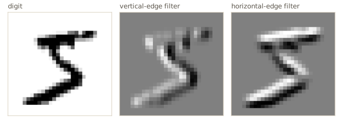
The kernels used in that check are the Sobel filters, a classical hand-designed pair. The vertical one computes a smoothed difference between the column to the right and the column to the left, so it responds to intensity changes as we move horizontally, which is where vertical edges are; its transpose responds to horizontal edges. The figure shows both applied to a digit. Where the intensity rises (dark to bright) the response is positive, and where it falls the response is negative. Look along one row through the middle of the digit:

edge_maps = conv2d(X[:1], torch.stack([sobel_v, sobel_h])[:, None], padding=1)[0]   # (2, 28, 28)
print("row 14 intensities, columns 8-19:   ", X[0, 0, 14, 8:20].numpy().round(1))
print("vertical-edge response, same pixels:", edge_maps[0, 14, 8:20].numpy().round(1))

row 14 intensities, columns 8-19:    [0.  0.  0.  0.  0.  0.3 0.9 1.  1.  0.5 0.1 0. ]
vertical-edge response, same pixels: [ 0.   0.   0.   0.1  1.6  2.8  1.8  0.5 -1.4 -2.6 -1.8 -0.8]

Three panels: an MNIST digit, its response to the vertical Sobel filter, and its response to the horizontal Sobel filter, shown in a diverging gray scale where positive responses are light and negative responses dark. — A training digit (left) and its responses to the vertical-edge (middle) and horizontal-edge (right) Sobel filters. Light means a positive response (intensity rising left to right, or top to bottom), dark a negative one; flat regions give zero. A convolutional network learns kernels like these instead of having them designed.

Seen as a matrix, a convolution is a very special dense layer. The next cell builds the matrix of a one-dimensional convolution with a width-3 kernel on six inputs, column by column, by feeding in unit vectors. Every row holds the same three weights, shifted one place: most entries are zero (sparse connections) and the nonzero ones repeat (shared weights). We will reuse conv_matrix when we meet transposed convolutions.

def conv_matrix(conv, in_shape):
    """Matrix A with conv(x).flatten() = A @ x.flatten(), built from unit inputs, one column each."""
    n = int(np.prod(in_shape))
    return torch.stack([conv(torch.eye(n)[i].view(in_shape)).flatten() for i in range(n)], dim=1)

A1d = conv_matrix(lambda x: conv2d(x, torch.tensor([1., 2., 3.]).view(1, 1, 1, 3)), (1, 1, 1, 6))
print(A1d.numpy())
print(f"{A1d.numel()} entries, {int((A1d != 0).sum())} nonzero, 3 distinct weights")

[[1. 2. 3. 0. 0. 0.]
 [0. 1. 2. 3. 0. 0.]
 [0. 0. 1. 2. 3. 0.]
 [0. 0. 0. 1. 2. 3.]]
24 entries, 12 nonzero, 3 distinct weights

Convolutions also bring a practical benefit: the number of parameters does not depend on the size of the image, so the same layer applies to images of any size, and all positions can be computed in parallel, which suits GPUs.

Note. Batch normalization (module 07) must respect the weight sharing. In a convolutional layer the mean and variance are computed per channel, over the batch and all spatial positions, and one pair of learned scale and shift parameters is used for the whole channel. Otherwise the statistics would depend on position and the layer would lose its equivariance. nn.BatchNorm2d does exactly this.

Padding

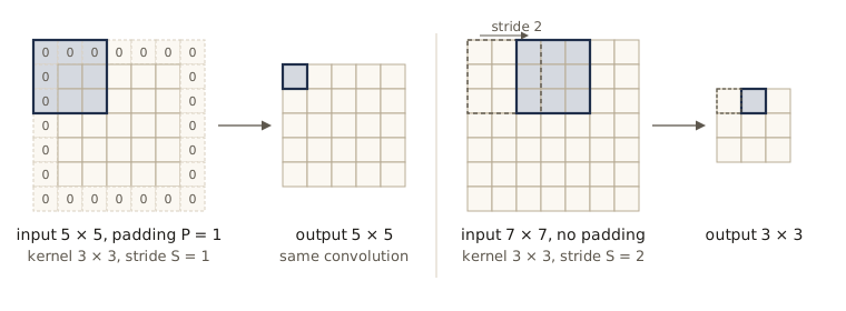
A valid convolution of a \(J \times K\) image with an \(M \times M\) kernel gives a \((J - M + 1) \times (K - M + 1)\) map, because the kernel must fit entirely inside the image. Stacking a few such layers shrinks the image quickly and gives the border pixels less influence than the central ones. The remedy is padding: surround the image with \(P\) extra pixels on every side before convolving, which gives a map of size \((J + 2P - M + 1) \times (K + 2P - M + 1)\).

Two choices have names. With \(P = 0\) the operation is a valid convolution. With \(P = (M - 1)/2\) the output has the same size as the input, a same convolution. This is one reason kernels almost always have an odd size: the padding is then symmetric and the kernel has a center pixel. The padding values are usually zeros, applied after the data have been shifted so that zero is a typical value (for MNIST, zero is already the background); PyTorch also offers reflected, replicated, and circular padding through the padding_mode argument of nn.Conv2d. Padding is used inside the network too, on feature maps.

for M in [3, 5, 7]:
    P = (M - 1) // 2
    same = F.conv2d(torch.zeros(1, 1, 28, 28), torch.zeros(1, 1, M, M), padding=P).shape[-1]
    print(f"M = {M}: same padding P = {P} keeps 28 -> {same};  valid (P = 0) gives {28 - M + 1}")

M = 3: same padding P = 1 keeps 28 -> 28;  valid (P = 0) gives 26
M = 5: same padding P = 2 keeps 28 -> 28;  valid (P = 0) gives 24
M = 7: same padding P = 3 keeps 28 -> 28;  valid (P = 0) gives 22

Strided convolutions

Sometimes we want a feature map much smaller than its input. One way is a strided convolution: instead of moving the kernel one pixel at a time, move it \(S\) pixels at a time. \(S\) is the stride.

To count the output positions along one axis, note that after padding the axis has \(J + 2P\) pixels, and the kernel’s first pixel can sit at positions \(0, S, 2S, \dots\) as long as the kernel still fits, that is, at \(qS \le J + 2P - M\). The number of such \(q \ge 0\) gives the output size

\[J_{\mathrm{out}} = \left\lfloor \frac{J + 2P - M}{S} \right\rfloor + 1,\]

and the same with \(K\) for the other axis, where \(\lfloor \cdot \rfloor\) rounds down. For large images the map is about \(1/S\) as wide as the image. We check the formula against PyTorch for 900 combinations of image size, kernel size, padding, and stride.

def out_size(J, M, P=0, S=1):
    """Side length of the feature map: floor((J + 2P - M) / S) + 1."""
    return (J + 2 * P - M) // S + 1

cases = mismatches = 0
for J in range(5, 20):
    for M in [1, 2, 3, 4, 5]:
        for P in [0, 1, 2]:
            for S in [1, 2, 3, 4]:
                got = F.conv2d(torch.zeros(1, 1, J, J), torch.zeros(1, 1, M, M),
                               stride=S, padding=P).shape[-1]
                cases += 1
                mismatches += int(got != out_size(J, M, P, S))
print(f"{cases} settings checked, {mismatches} mismatches")
print("28 x 28 image, 5 x 5 kernel, P = 2, S = 2 ->", out_size(28, 5, 2, 2), "x", out_size(28, 5, 2, 2))

900 settings checked, 0 mismatches
28 x 28 image, 5 x 5 kernel, P = 2, S = 2 -> 14 x 14

Watch out. Equation (10.5) of Bishop & Bishop is printed with \(-1\) inside the floor. The count derived above, with \(+1\) outside the floor, is the one that matches PyTorch in every case, and it reduces to \(J - M + 1\) for \(P = 0\) and \(S = 1\) as it should.

Two panels. Left: a 5 by 5 input surrounded by a ring of zero padding, a 3 by 3 kernel window in the top-left corner, and the resulting 5 by 5 output with the matching output cell highlighted. Right: a 7 by 7 input with the 3 by 3 window placed at stride 2, and the resulting 3 by 3 output. — Left: a same convolution. A 5 × 5 input with one ring of zero padding (P = 1) and a 3 × 3 kernel gives a 5 × 5 map; the highlighted window produces the highlighted output. Right: stride 2 without padding. The kernel jumps two pixels at a time over a 7 × 7 input, so the map is ⌊(7 − 3)/2⌋ + 1 = 3 wide.

Multi-dimensional convolutions

A color image has \(C = 3\) channels, and later layers have many more. A filter then becomes a small box of weights of size \(C \times M \times M\) (PyTorch puts the channel first), one \(M \times M\) slice per input channel, and the output at each position sums over all channels as well as over the patch:

\[a_{o}(j, k) = \sum_{c=1}^{C_{\mathrm{in}}} \sum_{l} \sum_{m} I_c(j + l, k + m)\, K_{oc}(l, m) + b_o .\]

One such filter is like a single hidden unit: it detects one kind of feature. To detect many kinds, a layer uses \(C_{\mathrm{out}}\) filters, each with its own weights and bias, producing \(C_{\mathrm{out}}\) feature maps, which are again called channels. The weights form a tensor of shape \(C_{\mathrm{out}} \times C_{\mathrm{in}} \times M \times M\), and the layer has

\[(M^2 C_{\mathrm{in}} + 1)\, C_{\mathrm{out}}\]

parameters, whatever the image size. A special case is worth knowing: the 1 × 1 convolution, with \(M = 1\). It applies the same linear map to the channel vector at every pixel, so it changes the number of channels without touching the spatial size. It is the channel counterpart of pooling and striding, which shrink the spatial size but leave the channels alone.

layer = nn.Conv2d(3, 16, kernel_size=3)
print("weight", tuple(layer.weight.shape), " bias", tuple(layer.bias.shape))
print("parameters:", sum(p.numel() for p in layer.parameters()),
      "  (M^2 C_in + 1) C_out =", (9 * 3 + 1) * 16)
X_rgb = torch.from_numpy(rng.random((2, 3, 12, 12))).float()
print("nn.Conv2d agrees with conv2d:", torch.allclose(layer(X_rgb), conv2d(X_rgb, layer.weight, layer.bias),
                                                     atol=1e-6))

one_by_one = nn.Conv2d(16, 4, kernel_size=1)
Z = torch.from_numpy(rng.normal(size=(2, 16, 10, 10))).float()
mix = torch.einsum("oc,nchw->nohw", one_by_one.weight[:, :, 0, 0], Z) + one_by_one.bias.view(1, -1, 1, 1)
print("1x1 convolution = one linear map of the channels at every pixel:",
      torch.allclose(one_by_one(Z), mix, atol=1e-6), "  output", tuple(one_by_one(Z).shape))

weight (16, 3, 3, 3)  bias (16,)
parameters: 448   (M^2 C_in + 1) C_out = 448
nn.Conv2d agrees with conv2d: True
1x1 convolution = one linear map of the channels at every pixel: True   output (2, 4, 10, 10)

Pooling

Equivariance is what we want when the output is itself a map, for instance when we need to know where a feature is. For a class label we want the opposite, invariance: moving the digit by a pixel should not change the answer. Complex features are made of simpler ones in roughly the right arrangement (the loop of a 9 above its stem), but the exact position of each part should not matter much.

A pooling layer provides a degree of this. Like a convolution it has a grid of units, each looking at a small window of the previous map with some window size and stride, but each unit computes a fixed function with no learnable parameters. Max-pooling outputs the largest value in its window; average pooling outputs the mean. With a \(2 \times 2\) window and stride 2 the windows do not overlap and each side of the map halves. Pooling acts on each channel separately, so eight \(64 \times 64\) channels become eight \(32 \times 32\) channels.

If a feature map measures how strongly a feature is present at each position, max-pooling keeps “is it present in this region, and how strongly” and discards exactly where in the region it was. The function below uses the same patch view as conv2d.

def pool2d(X, size=2, stride=2, kind="max"):
    """Max or average pooling of each channel separately."""
    patches = X.unfold(2, size, stride).unfold(3, size, stride)      # (N, C, H_out, W_out, size, size)
    return patches.amax(dim=(-2, -1)) if kind == "max" else patches.mean(dim=(-2, -1))

A4 = torch.tensor([[[[2., 7., 1., 0.], [4., 3., 5., 8.], [6., 1., 0., 2.], [9., 3., 4., 4.]]]])
print("input:\n", A4[0, 0].numpy())
print("2x2 max pool:\n", pool2d(A4)[0, 0].numpy(), "\n2x2 average pool:\n", pool2d(A4, kind="avg")[0, 0].numpy())
Zp = torch.from_numpy(rng.normal(size=(2, 3, 9, 11))).float()
print("agree with F.max_pool2d / F.avg_pool2d (3x3 windows, stride 2):",
      torch.allclose(pool2d(Zp, 3, 2), F.max_pool2d(Zp, 3, 2)),
      torch.allclose(pool2d(Zp, 3, 2, "avg"), F.avg_pool2d(Zp, 3, 2)))

input:
 [[2. 7. 1. 0.]
 [4. 3. 5. 8.]
 [6. 1. 0. 2.]
 [9. 3. 4. 4.]]
2x2 max pool:
 [[7. 8.]
 [9. 4.]] 
2x2 average pool:
 [[4.   3.5 ]
 [4.75 2.5 ]]
agree with F.max_pool2d / F.avg_pool2d (3x3 windows, stride 2): True True

How much invariance does pooling buy? We compute the Sobel edge maps (after a ReLU) of 500 digits, shift every digit one pixel to the right, and measure the relative change in the features with no pooling, with max-pooling over larger and larger windows, and with a single maximum over the whole map (global max-pooling).

edge_bank = torch.stack([sobel_v, sobel_h])[:, None]                      # (2, 1, 3, 3)
feats = conv2d(X[:500], edge_bank, padding=1).relu()
feats_moved = conv2d(torch.roll(X[:500], 1, dims=3), edge_bank, padding=1).relu()
poolers = [("no pooling", lambda z: z), ("2x2 max pool", lambda z: pool2d(z, 2, 2)),
           ("4x4 max pool", lambda z: pool2d(z, 4, 4)), ("7x7 max pool", lambda z: pool2d(z, 7, 7)),
           ("global max", lambda z: z.amax(dim=(2, 3)))]
for name, f in poolers:
    change = ((f(feats_moved) - f(feats)).norm() / f(feats).norm()).item()
    print(f"{name:13s} relative change after a one-pixel shift: {change:.3f}")

no pooling    relative change after a one-pixel shift: 0.722
2x2 max pool  relative change after a one-pixel shift: 0.537
4x4 max pool  relative change after a one-pixel shift: 0.361
7x7 max pool  relative change after a one-pixel shift: 0.286
global max    relative change after a one-pixel shift: 0.000

Without pooling, a one-pixel shift changes the edge features by about 70% of their size, because a thin edge moves off most of the pixels it was on. Each larger pooling window roughly halves the remaining sensitivity, and the global maximum does not change at all (moving the whole digit inside the frame cannot change the largest response). Between those extremes the invariance is only approximate: a shift that moves a feature across a window boundary still changes the pooled value.

Pooling also appears in two other roles. Pooling across channels, for example taking the maximum over several channels that detect the same pattern at different orientations, can make a network approximately invariant to other transformations such as rotations. And adaptive pooling, which chooses the window size from the input size so that the output always has a fixed shape, lets one network accept images of different sizes:

adaptive = nn.AdaptiveMaxPool2d((4, 4))
print({side: tuple(adaptive(torch.zeros(1, 16, side, side)).shape) for side in [28, 40, 57]})

{28: (1, 16, 4, 4), 40: (1, 16, 4, 4), 57: (1, 16, 4, 4)}

Multilayer convolutions

One convolutional layer, perhaps followed by pooling, plays the role of one layer of a fully connected network. To learn a hierarchy we stack them: layer \(l\) has a weight tensor of shape \(C_{\mathrm{out}} \times C_{\mathrm{in}} \times M \times M\) with \((M^2 C_{\mathrm{in}} + 1) C_{\mathrm{out}}\) parameters, and its output channels are the input channels of layer \(l + 1\), just as the red, green, and blue channels are the input of the first layer. (The number of channels is sometimes called the depth of a feature map; we keep “depth” for the number of layers.)

Every unit sees only a small window of the layer below, but that window sees a window of the layer below it, and so on. The effective receptive field of a unit, the region of the input image that can influence it, therefore grows with depth. Let \(r_l\) be the receptive field size after layer \(l\) and \(j_l\) the jump, the distance in input pixels between neighboring units of layer \(l\). A layer with kernel \(M_l\) and stride \(S_l\) adds \(M_l - 1\) neighbors, each \(j_{l-1}\) input pixels apart, so

\[r_l = r_{l-1} + (M_l - 1)\, j_{l-1}, \qquad j_l = j_{l-1} S_l, \qquad r_0 = j_0 = 1 .\]

Pooling layers follow the same rule, with their window size as \(M_l\). We compute this for the LeNet-style network trained below (5 × 5 convolution, 2 × 2 pooling, 5 × 5 convolution, 2 × 2 pooling), and check each value by building a network with all-ones kernels and average pooling and looking at which input pixels have a nonzero gradient for one unit in the middle.

def receptive_field(layers):
    """layers: list of (kind, M, S). Returns receptive field r and jump j in input pixels."""
    r, j = 1, 1
    for _, M, S in layers:
        r, j = r + (M - 1) * j, j * S
    return r, j

def measured_field(layers, side=48):
    """Width of the set of input pixels with nonzero gradient for the central unit of the last layer."""
    x = torch.zeros(1, 1, side, side, requires_grad=True)
    h = x
    for kind, M, S in layers:
        h = F.conv2d(h, torch.ones(1, 1, M, M), stride=S) if kind == "conv" else F.avg_pool2d(h, M, S)
    c = h.shape[-1] // 2
    g, = torch.autograd.grad(h[0, 0, c, c], x)
    cols = (g[0, 0].abs().sum(0) > 0).nonzero()
    return (cols.max() - cols.min() + 1).item()

lenet_layers = [("conv", 5, 1), ("pool", 2, 2), ("conv", 5, 1), ("pool", 2, 2)]
for depth in range(1, 5):
    r, j = receptive_field(lenet_layers[:depth])
    print(f"after {depth} layer(s): receptive field {r:2d} (measured {measured_field(lenet_layers[:depth]):2d}),"
          f" jump {j}")

after 1 layer(s): receptive field  5 (measured  5), jump 1
after 2 layer(s): receptive field  6 (measured  6), jump 2
after 3 layer(s): receptive field 14 (measured 14), jump 2
after 4 layer(s): receptive field 16 (measured 16), jump 4

A unit after the second pooling layer sees a \(16 \times 16\) region, more than half of a 28-pixel digit, although no kernel is larger than \(5 \times 5\).

Large receptive fields can come either from large kernels or from stacks of small ones. Stacks are cheaper and more expressive: two \(3 \times 3\) layers see a \(5 \times 5\) region with fewer parameters than one \(5 \times 5\) layer, and three see \(7 \times 7\), with a nonlinearity between each pair. With \(C\) channels in and out:

C = 64
for n, M in [(2, 5), (3, 7)]:
    stack = n * (9 * C + 1) * C
    single = (M * M * C + 1) * C
    print(f"{n} stacked 3x3 layers: receptive field {receptive_field([('conv', 3, 1)] * n)[0]},"
          f" {stack:,} parameters;  one {M}x{M} layer: {single:,} parameters")

2 stacked 3x3 layers: receptive field 5, 73,856 parameters;  one 5x5 layer: 102,464 parameters
3 stacked 3x3 layers: receptive field 7, 110,784 parameters;  one 7x7 layer: 200,768 parameters

For classification the output must depend on the whole image, so the last stages of a CNN are usually one or two fully connected layers, or a global pooling followed by one. Because pooling has shrunk the maps by then, these layers stay affordable, yet they often hold most of the network’s parameters, while the convolutional layers perform most of the computation, since their few weights are reused at every position.

A full CNN is therefore a sequence of convolutions interleaved with pooling, ending in fully connected layers. Its designer chooses the number of layers, the channels per layer, kernel sizes, strides, and more. Each candidate costs a full training run, so these choices are rarely searched systematically; in practice one adapts an architecture that is known to work.

Example network architectures

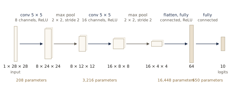
The first networks with more than two layers of learnable weights to see practical use were convolutional. The classic early example is LeNet, developed by Yann LeCun and colleagues around 1989 and described fully in a 1998 paper, which read handwritten digits. We build a small network in that style for MNIST: two valid \(5 \times 5\) convolutions with 8 and 16 channels, each followed by a ReLU and \(2 \times 2\) max-pooling, then a fully connected layer of 64 units and 10 outputs. We split the forward pass into features (up to the pre-activations of the last convolutional layer) and head (the rest), because several later sections need the last feature maps.

class LeNet(nn.Module):
    """conv 5x5 (8) -> ReLU -> pool 2 -> conv 5x5 (16) -> ReLU -> pool 2 -> FC 64 -> ReLU -> FC 10."""

    def __init__(self):
        super().__init__()
        self.conv1 = nn.Conv2d(1, 8, 5)             # 28 x 28 -> 24 x 24
        self.conv2 = nn.Conv2d(8, 16, 5)            # 12 x 12 -> 8 x 8
        self.fc1 = nn.Linear(16 * 4 * 4, 64)
        self.fc2 = nn.Linear(64, 10)

    def features(self, x):
        """Pre-activations a_ijk of the last convolutional layer, shape (N, 16, 8, 8)."""
        return self.conv2(F.max_pool2d(F.relu(self.conv1(x)), 2))

    def head(self, a):
        """From last-layer pre-activations to the class logits a^(c) (before the softmax)."""
        z = F.max_pool2d(F.relu(a), 2).flatten(1)
        return self.fc2(F.relu(self.fc1(z)))

    def forward(self, x):
        return self.head(self.features(x))

torch.manual_seed(10)
cnn = LeNet()
h = X[:1]
steps = [("conv1 (5x5, 8 channels)", cnn.conv1), ("ReLU, 2x2 max pool", lambda z: F.max_pool2d(F.relu(z), 2)),
         ("conv2 (5x5, 16 channels)", cnn.conv2), ("ReLU, 2x2 max pool", lambda z: F.max_pool2d(F.relu(z), 2)),
         ("flatten", lambda z: z.flatten(1)), ("fc1 + ReLU", lambda z: F.relu(cnn.fc1(z))),
         ("fc2 (logits)", cnn.fc2)]
print(f"{'input':26s} {tuple(h.shape)}")
for name, f in steps:
    h = f(h)
    print(f"{name:26s} {tuple(h.shape)}")
for name, p in cnn.named_parameters():
    if name.endswith("weight"):
        print(f"{name[:-7]:6s} parameters (with bias): {p.numel() + p.shape[0]:6,d}")
print(f"total: {sum(p.numel() for p in cnn.parameters()):,}")

input                      (1, 1, 28, 28)
conv1 (5x5, 8 channels)    (1, 8, 24, 24)
ReLU, 2x2 max pool         (1, 8, 12, 12)
conv2 (5x5, 16 channels)   (1, 16, 8, 8)
ReLU, 2x2 max pool         (1, 16, 4, 4)
flatten                    (1, 256)
fc1 + ReLU                 (1, 64)
fc2 (logits)               (1, 10)
conv1  parameters (with bias):    208
conv2  parameters (with bias):  3,216
fc1    parameters (with bias): 16,448
fc2    parameters (with bias):    650
total: 20,522

Diagram of the LeNet-style network as a row of blocks: a 1 by 28 by 28 input, a 5 by 5 convolution to 8 by 24 by 24, 2 by 2 max pooling to 8 by 12 by 12, a 5 by 5 convolution to 16 by 8 by 8, max pooling to 16 by 4 by 4, a fully connected layer of 64 units, and 10 outputs. Parameter counts are written under each learnable layer. — The LeNet-style network used in this module, with the shape of every feature map (channels × height × width) and the parameters of each learnable layer. The two convolutional layers have 3,424 parameters between them; the first fully connected layer alone has 16,448.

For comparison we use a fully connected network with one hidden layer of 100 ReLU units, which has almost four times as many parameters. Both are trained with Adam on the cross-entropy error, in mini-batches of 64.

@torch.no_grad()
def accuracy(model, X, y):
    return (model(X).argmax(1) == y).float().mean().item()

def train(model, X, y, epochs, lr=2e-3, batch=64, seed=0, log_every=1):
    """Mini-batch Adam on the cross-entropy error; prints test accuracy every log_every epochs."""
    gen = torch.Generator().manual_seed(seed)
    opt = torch.optim.Adam(model.parameters(), lr=lr)
    for epoch in range(1, epochs + 1):
        for idx in torch.randperm(len(X), generator=gen).split(batch):
            loss = F.cross_entropy(model(X[idx]), y[idx])
            opt.zero_grad()
            loss.backward()
            opt.step()
        if epoch % log_every == 0:
            print(f"  epoch {epoch:2d}   last-batch loss {loss.item():.3f}"
                  f"   test accuracy {accuracy(model, X_test, y_test):.4f}")
    return model

print("CNN,", sum(p.numel() for p in cnn.parameters()), "parameters")
t0 = time.perf_counter()
train(cnn, X, y, epochs=5)
t_cnn = time.perf_counter() - t0

torch.manual_seed(10)
mlp = nn.Sequential(nn.Flatten(), nn.Linear(784, 100), nn.ReLU(), nn.Linear(100, 10))
print("MLP,", sum(p.numel() for p in mlp.parameters()), "parameters")
t0 = time.perf_counter()
train(mlp, X, y, epochs=15, log_every=5)
t_mlp = time.perf_counter() - t0
print(f"training time (your times will differ): CNN {t_cnn:.1f} s for 5 epochs,"
      f" MLP {t_mlp:.1f} s for 15 epochs")

CNN, 20522 parameters
  epoch  1   last-batch loss 0.521   test accuracy 0.8705
  epoch  2   last-batch loss 0.138   test accuracy 0.9145
  epoch  3   last-batch loss 0.164   test accuracy 0.9270
  epoch  4   last-batch loss 0.269   test accuracy 0.9310
  epoch  5   last-batch loss 0.088   test accuracy 0.9425
MLP, 79510 parameters
  epoch  5   last-batch loss 0.189   test accuracy 0.9015
  epoch 10   last-batch loss 0.037   test accuracy 0.9100
  epoch 15   last-batch loss 0.012   test accuracy 0.9175
training time (your times will differ): CNN 7.1 s for 5 epochs, MLP 3.4 s for 15 epochs

With a quarter of the parameters, the CNN is clearly more accurate than the fully connected network, even when the latter trains for three times as many epochs. The price is computation: every convolutional weight is used at hundreds of positions, so an epoch of the small CNN takes several times longer than an epoch of the larger MLP. On the full 60,000 training images, with a few more channels and some data augmentation, networks of this kind reach well above 99% test accuracy; that needs a GPU or much more patience than our budget allows.

The ImageNet era. Progress beyond digits was driven by ImageNet, a data set of millions of labeled natural photographs, and by the annual ImageNet Large Scale Visual Recognition Challenge, which used a subset with 1,000 classes and reported top-1 and top-5 error (the true class must be the first guess, or among the five highest-ranked guesses). The network that won the 2012 challenge, AlexNet (Krizhevsky, Sutskever, and Hinton), was a large CNN trained on GPUs with ReLU activations and dropout, and its margin of victory is widely seen as the start of the deep learning era in vision. Its first layer used large \(11 \times 11\) kernels with stride 4.

VGG-16 (Simonyan and Zisserman, 2014) showed how far a very regular design goes. Every convolution is \(3 \times 3\) with stride 1 and same padding, followed by a ReLU; every pooling is \(2 \times 2\) max-pooling with stride 2; and each time the maps halve in size, the number of channels doubles (64, 128, 256, 512, then 512 again), so the amount of information per layer shrinks only slowly. Thirteen convolutional layers on a \(224 \times 224 \times 3\) input end in a \(7 \times 7 \times 512\) map, followed by fully connected layers of 4,096, 4,096, and 1,000 units. We can count its parameters from that description with the formula of this section:

vgg_blocks = [(64, 2), (128, 2), (256, 3), (512, 3), (512, 3)]    # (channels, conv layers) per block
c_in, conv_params, layers = 3, 0, []
for c, n in vgg_blocks:
    for _ in range(n):
        conv_params += (9 * c_in + 1) * c
        c_in = c
        layers.append(("conv", 3, 1))
    layers.append(("pool", 2, 2))
fc_sizes = [7 * 7 * 512, 4096, 4096, 1000]
fc_params = [(a + 1) * b for a, b in zip(fc_sizes[:-1], fc_sizes[1:])]
print(f"convolutional layers: {conv_params:,} parameters")
print(f"fully connected layers: {sum(fc_params):,} (the first alone: {fc_params[0]:,})")
print(f"total: {conv_params + sum(fc_params):,}")
print("receptive field of the last convolutional layer:", receptive_field(layers[:-1])[0], "pixels")

convolutional layers: 14,714,688 parameters
fully connected layers: 123,642,856 (the first alone: 102,764,544)
total: 138,357,544
receptive field of the last convolutional layer: 196 pixels

About 138 million parameters, three quarters of them in the first fully connected layer, and a last convolutional layer whose units each see a 196-pixel square, most of the 224-pixel input. Later designs removed most of those fully connected parameters by ending with global average pooling, and residual networks (ResNets, He et al., 2016) made networks with many dozens of layers trainable by adding skip connections around small groups of layers; residual connections are covered with the other regularizing architectural choices in module 09. However complex the architecture, we only write the forward pass: automatic differentiation (module 08) supplies the gradients, and the training loop is the one above.

Visualizing trained CNNs

What has a trained network learned? For a CNN we can look, because the early layers work in image space.

Visual cortex

Much of the inspiration for convolutional networks came from neuroscience. In the visual cortex, signals from the retina pass through a series of processing stages whose neurons are laid out in sheets that map the visual field. In experiments beginning in 1959, David Hubel and Torsten Wiesel recorded the electrical activity of single cells in the cat visual cortex as the animals were shown simple patterns. They found simple cells that respond strongly to an edge or bar at a particular orientation and position and hardly at all to other stimuli, and complex cells that respond to similar patterns but tolerate small shifts of position, much like a pooling unit. Cells further along the pathway respond to more specific patterns with more invariance; the half-joking name “grandmother cell” was coined for a hypothetical neuron that would fire for one particular person whatever the viewpoint or lighting.

The responses of simple cells are well described by Gabor functions, sinusoids at some orientation multiplied by a Gaussian envelope:

\[G(x, y) = A \exp\left(-\alpha \tilde{x}^2 - \beta \tilde{y}^2\right) \sin(\omega \tilde{x} + \phi),\]

where \(\tilde{x} = (x - x_0)\cos\theta + (y - y_0)\sin\theta\) and \(\tilde{y} = -(x - x_0)\sin\theta + (y - y_0)\cos\theta\) rotate the coordinates by \(\theta\) about the center \((x_0, y_0)\). The sine oscillates across the direction \(\theta\) with frequency \(\omega\) and phase \(\phi\), and \(\alpha\) and \(\beta\) set how quickly the envelope decays. Used as a convolution kernel, a Gabor function is an oriented edge or bar detector. Here are four orientations applied to all training images of three digit classes:

def gabor(theta, omega=1.0, phi=0.0, alpha=0.06, beta=0.06, size=9):
    """Gabor kernel exp(-alpha xt^2 - beta yt^2) sin(omega xt + phi), coordinates rotated by theta."""
    r = torch.arange(size) - (size - 1) / 2
    yy, xx = torch.meshgrid(r, r, indexing="ij")
    xt = xx * math.cos(theta) + yy * math.sin(theta)
    yt = -xx * math.sin(theta) + yy * math.cos(theta)
    return torch.exp(-alpha * xt ** 2 - beta * yt ** 2) * torch.sin(omega * xt + phi)

angles = [0, 45, 90, 135]
bank = torch.stack([gabor(math.radians(a)) for a in angles])[:, None]     # (4, 1, 9, 9)
print("mean ReLU response per orientation (degrees):", angles)
for digit in [0, 1, 7]:
    resp = conv2d(X[y == digit], bank, padding=4).relu().mean(dim=(0, 2, 3))
    print(f"  digit {digit}:", resp.numpy().round(3))

mean ReLU response per orientation (degrees): [0, 45, 90, 135]
  digit 0: [0.676 0.822 0.589 0.525]
  digit 1: [0.513 0.445 0.177 0.222]
  digit 7: [0.494 0.629 0.486 0.331]

With \(\theta = 0\) the sine varies along \(x\), so the kernel detects vertical strokes, and it dominates for the mostly vertical 1s. At 45° the stripes of the kernel run from bottom left to top right (rows count downward), the direction of the long stroke of a 7, which is the orientation sevens prefer. Zeros, with curved strokes in every direction, respond to all four orientations, and no single one stands out as much.

These findings inspired the neocognitron of Kunihiko Fukushima (1980), a multilayer network with local receptive fields, shared weights, and pooling, and a direct ancestor of CNNs. It was trained layer by layer with an unsupervised rule rather than end to end, because it predated the widespread use of backpropagation.

Visualizing trained filters

The first-layer kernels of a CNN multiply image patches directly, so they can be displayed as images. For networks trained on large sets of natural photographs, many first-layer filters look strikingly like Gabor functions: oriented edges and bars at several scales, plus color blobs. That resemblance is not evidence that CNNs work like brains. Many quite different statistical methods applied to natural images produce similar filters, because such filters reflect the statistics of natural images themselves.

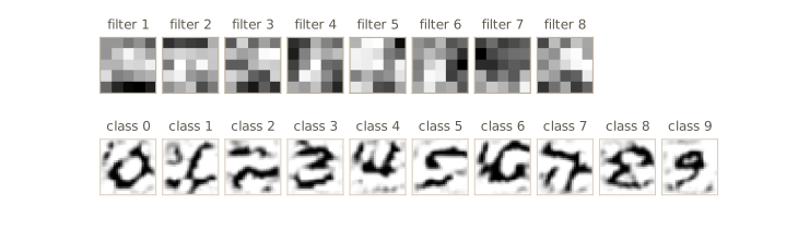
Our network saw only digits, and its eight \(5 \times 5\) filters are shown in the top row of the next figure. They are rougher, but several are clearly oriented stroke and edge detectors. We can also run the Hubel–Wiesel experiment on the network: search 1,000 training images for the patch that drives each filter hardest, and compare that patch with the filter itself. By the feature-detector argument above, the best patch should resemble the kernel.

W1, b1 = cnn.conv1.weight.detach()[:, 0], cnn.conv1.bias.detach()          # (8, 5, 5), (8,)
patches = X[:1000].unfold(2, 5, 1).unfold(3, 5, 1).reshape(-1, 25)          # every 5x5 patch
pre = patches @ W1.reshape(8, 25).T + b1                                     # pre-activations
top = patches[pre.argmax(0)]                                                 # best patch per filter
cos = F.cosine_similarity(top, W1.reshape(8, 25), dim=1)
cos_all = F.cosine_similarity(patches[:, None, :], W1.reshape(1, 8, 25), dim=2)
print(f"{patches.shape[0]:,} patches searched")
print("cosine(best patch, filter):         ", cos.numpy().round(2))
print("99.9th percentile over all patches: ", torch.quantile(cos_all[:200_000], 0.999, dim=0).numpy().round(2))

576,000 patches searched
cosine(best patch, filter):          [0.66 0.77 0.57 0.54 0.82 0.63 0.44 0.73]
99.9th percentile over all patches:  [0.67 0.75 0.59 0.6  0.79 0.68 0.46 0.73]

For every filter the best patch has a cosine similarity with the kernel close to the 99.9th percentile over all patches, so it does look like the filter. It is not always the single most similar patch, because the pre-activation also rewards bright patches (a large \(\lVert \mathbf{x} \rVert\)), which is why the argument above fixed the norm.

Top row: eight small 5 by 5 gray-scale images of the trained network's first-layer filters, showing oriented light and dark bands. Bottom row: ten 28 by 28 images synthesized by maximizing each digit class logit, labeled 0 to 9, which show faint stroke-like patterns resembling the digits. — Top: the eight first-layer filters of the trained CNN (light = positive weight). Several are oriented stroke or edge detectors. Bottom: an input synthesized for each class by gradient ascent on that class's logit with a small penalty on pixel size (see "Synthetic images" below). The strokes that the network relies on for each digit are visible.

Deeper layers are harder to show, because their inputs are channels of earlier features rather than pixels. One approach, used by Zeiler and Fergus (2013) on a large ImageNet network, is the same search as above: collect the image patches (within each unit’s receptive field) that most excite a unit. Their collections progress from edges in the first layer to textures and simple shapes, then parts of objects, and whole objects in the fifth layer. Another approach synthesizes an input by optimization, which we do below.

Saliency maps

A saliency map highlights the pixels or regions that mattered most for a particular decision. The simplest version is the gradient of the class’s logit \(a^{(c)}\) (the pre-softmax output) with respect to the input pixels: if \(\lvert \partial a^{(c)} / \partial x_i \rvert\) is large, a small change to pixel \(i\) changes the score a lot.

Pixel gradients tend to be noisy. Grad-CAM (gradient-weighted class activation mapping, Selvaraju et al.) works one level up, at the last convolutional layer, which still knows where things are but already represents high-level features. Let \(a^{(k)}_{ij}\) be the unit at row \(i\), column \(j\) of channel \(k\) in that layer, and \(M_k\) the number of positions in the channel. Grad-CAM weighs each channel by the average gradient of the class logit with respect to it,

\[\alpha_k = \frac{1}{M_k} \sum_{i} \sum_{j} \frac{\partial a^{(c)}}{\partial a^{(k)}_{ij}},\]

and forms the map \(L = \sum_k \alpha_k \mathbf{A}^{(k)}\), where \(\mathbf{A}^{(k)}\) is the matrix with entries \(a^{(k)}_{ij}\). The map has the resolution of that layer (here \(8 \times 8\)) and is up-sampled onto the image for display. Bishop & Bishop state the method with the layer’s pre-activations; the original paper uses the activations after the ReLU and also applies a ReLU to \(L\), keeping only positive evidence for the class. We follow the original, which gives cleaner maps for our small network.

def input_saliency(model, X, c):
    """|d a^(c) / d x| for each image of a batch; c holds one class per image."""
    X = X.clone().requires_grad_(True)
    logits = model(X)
    g, = torch.autograd.grad(logits[torch.arange(len(X)), c].sum(), X)
    return g.abs()[:, 0]

def grad_cam(model, x, c):
    """Grad-CAM map ReLU(sum_k alpha_k A^(k)) at the last convolutional layer, for one image."""
    A = F.relu(model.features(x)).detach().requires_grad_(True)  # rectified maps, (1, 16, 8, 8)
    dA, = torch.autograd.grad(model.head(A)[0, c], A)            # head's ReLU leaves A unchanged
    alpha = dA.mean(dim=(2, 3), keepdim=True)                    # average gradient per channel
    return F.relu((alpha * A).sum(1)[0]).detach()

S = input_saliency(cnn, X_test[:200], y_test[:200])
ink = X_test[:200, 0] > 0.2
print(f"ink covers {ink.float().mean().item():.1%} of the pixels"
      f" but receives {(S * ink).sum().item() / S.sum().item():.1%} of the gradient saliency")
L = grad_cam(cnn, X_test[:1], y_test[0].item())
print(f"Grad-CAM for the first test image (a {y_test[0].item()}), 8 x 8, divided by its maximum:")
print((L / L.max()).numpy().round(1))

ink covers 14.9% of the pixels but receives 41.6% of the gradient saliency
Grad-CAM for the first test image (a 7), 8 x 8, divided by its maximum:
[[0.  0.1 0.1 0.2 0.2 0.2 0.2 0.3]
 [0.  0.  0.  0.  0.  0.  0.1 0.4]
 [0.5 0.5 0.5 0.4 0.5 0.4 0.1 0.6]
 [0.5 0.6 0.6 0.6 0.4 0.4 0.3 0.8]
 [0.2 0.3 0.2 0.3 0.4 0.2 0.7 0.9]
 [0.1 0.1 0.2 0.4 0.3 0.4 1.  0.7]
 [0.1 0.1 0.3 0.4 0.1 0.9 0.9 0.4]
 [0.  0.3 0.4 0.2 0.6 1.  0.7 0.2]]

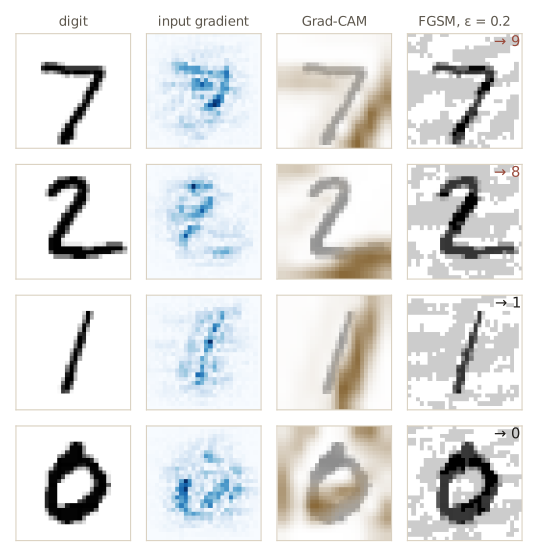
The input gradient concentrates on the strokes, with almost three times their share of the pixels. The Grad-CAM map is coarse, since each of its cells stands for a 14-pixel square of the input, and the figure below shows that for our small network it often puts its weight next to the strokes rather than on them: the evidence for a class includes where ink is absent (the open space to the right of a 1, the gap under the bar of a 7). Saliency maps describe the network, not the digit, and they are easy to over-read.

Is the saliency meaningful? A standard test is deletion: remove the pixels the map calls most important and see whether the network notices more than when removing the same number of other pixels. We blank the 30 most salient pixels of each image, and for comparison 30 randomly chosen ink pixels.

def blank(X, idx):
    Xb = X.clone().flatten(1)
    Xb[torch.arange(len(X))[:, None], idx] = 0.0
    return Xb.view_as(X)

k, gen = 30, torch.Generator().manual_seed(1)
salient = S.flatten(1).topk(k, dim=1).indices
noise = torch.rand(ink.flatten(1).shape, generator=gen) + ink.flatten(1).float()   # ink pixels rank first
random_ink = noise.topk(k, dim=1).indices
for name, idx in [("no pixels removed", None), (f"{k} most salient pixels", salient),
                  (f"{k} random ink pixels", random_ink)]:
    Xd = X_test[:200] if idx is None else blank(X_test[:200], idx)
    print(f"{name:24s} accuracy {accuracy(cnn, Xd, y_test[:200]):.3f}")

no pixels removed        accuracy 0.995
30 most salient pixels   accuracy 0.720
30 random ink pixels     accuracy 0.980

A grid with four rows, one per test digit, and four columns: the digit, its input-gradient saliency map, its Grad-CAM map overlaid on the digit, and the digit after a fast-gradient-sign attack with epsilon 0.2, labeled with the network's new prediction. — Four test digits (first column), the magnitude of the gradient of the true class's logit with respect to each pixel (second), the Grad-CAM map for the true class, up-sampled from 8 × 8 and drawn over the digit (third; brown = positive evidence), and the same digit after an FGSM attack with ε = 0.2, labeled with the network's prediction, in rust when it is wrong (fourth).

Adversarial attacks

The same input gradients can be turned against the network. Szegedy et al. (2013) found that tiny, carefully chosen changes to an image, too small for a person to notice on high-resolution photographs, can make a network misclassify it. The fast gradient sign method (FGSM) of Goodfellow, Shlens, and Szegedy (2014) builds such a change in one step. Move every pixel by the same small amount \(\epsilon\) in the direction that increases the error \(E(\mathbf{x}, t)\) for the true label \(t\):

\[\mathbf{x}' = \mathbf{x} + \epsilon \operatorname{sign}\left(\nabla_{\mathbf{x}} E(\mathbf{x}, t)\right).\]

This is one step of gradient ascent on the error, taken with respect to the input while the weights stay fixed; training does the opposite, descending with respect to the weights. We also clip \(\mathbf{x}'\) to the valid range \([0, 1]\).

Why does such a small change work? Look at one linear unit, \(a = \mathbf{w}^{\mathrm{T}}\mathbf{x}\), and a perturbation \(\boldsymbol{\eta}\) whose entries are at most \(\epsilon\) in size. The largest possible change of \(a\) is

\[\max_{\lVert \boldsymbol{\eta} \rVert_\infty \le \epsilon} \mathbf{w}^{\mathrm{T}}\boldsymbol{\eta} = \epsilon \lVert \mathbf{w} \rVert_1 = \epsilon \sum_{i=1}^{D} \lvert w_i \rvert,\]

reached by \(\boldsymbol{\eta} = \epsilon \operatorname{sign}(\mathbf{w})\). It grows in proportion to the dimension \(D\), although no single pixel changes by more than \(\epsilon\). A random choice of signs instead gives a change with mean zero and standard deviation \(\epsilon \lVert \mathbf{w} \rVert_2\), which grows only like \(\sqrt{D}\). In high dimensions, many small coordinated changes add up. FGSM applies this linear reasoning to the network’s local linearization, with \(\mathbf{w}\) replaced by the gradient.

def fgsm(model, X, y, eps):
    """x' = x + eps * sign(grad_x E(x, t)), clipped to the pixel range [0, 1]."""
    X = X.clone().requires_grad_(True)
    g, = torch.autograd.grad(F.cross_entropy(model(X), y, reduction="sum"), X)
    return (X + eps * g.sign()).clamp(0, 1).detach()

def random_sign(X, eps, seed=0):
    gen = torch.Generator().manual_seed(seed)
    return (X + eps * (torch.randint(0, 2, X.shape, generator=gen) * 2 - 1)).clamp(0, 1)

print(" eps    CNN (FGSM)   MLP (FGSM)   CNN (random signs)")
for eps in [0.0, 0.05, 0.1, 0.15, 0.2, 0.25]:
    print(f"{eps:4.2f}   {accuracy(cnn, fgsm(cnn, X_test, y_test, eps), y_test):10.3f}"
          f"   {accuracy(mlp, fgsm(mlp, X_test, y_test, eps), y_test):10.3f}"
          f"   {accuracy(cnn, random_sign(X_test, eps), y_test):16.3f}")

g_c = input_saliency(cnn, X_test[:200], y_test[:200]).flatten(1)      # gradient magnitudes
ratio = (g_c.sum(1) / g_c.norm(dim=1)).mean().item()
print(f"mean of norm1(g) / norm2(g) for the CNN logit gradient: {ratio:.1f} (upper bound sqrt(D) = 28)")

 eps    CNN (FGSM)   MLP (FGSM)   CNN (random signs)
00        0.942        0.918              0.942
05        0.849        0.352              0.939
10        0.643        0.036              0.938
15        0.358        0.007              0.932
20        0.138        0.002              0.919
25        0.036        0.002              0.900
mean of norm1(g) / norm2(g) for the CNN logit gradient: 15.4 (upper bound sqrt(D) = 28)

The fully connected network collapses almost at once: at \(\epsilon = 0.05\) it is right on only about a third of the digits, and at 0.1 on almost none. The CNN resists longer but not for long. A perturbation of 0.1 per pixel (a tenth of the intensity range) costs it about a third of its accuracy, and at 0.25 it is wrong on nearly every digit, while random signs of the same size barely matter. The ratio in the last line is the linear argument in numbers: the attack’s first-order effect is about 15 standard deviations of the effect of random noise of the same size. On 28 × 28 digits the attacked images still look like the original digits with gray speckle; on large color photographs, where \(D\) is in the hundreds of thousands, far smaller values of \(\epsilon\) suffice and the change is invisible.

Adversarial images often transfer: an image crafted against one network also fools a different network trained for the same task.

X_adv_mlp = fgsm(mlp, X_test, y_test, 0.15)
print(f"CNN accuracy on images attacked through the MLP (eps = 0.15): {accuracy(cnn, X_adv_mlp, y_test):.3f}")
print(f"CNN accuracy on random-sign noise of the same size:            "
      f"{accuracy(cnn, random_sign(X_test, 0.15), y_test):.3f}")

CNN accuracy on images attacked through the MLP (eps = 0.15): 0.714
CNN accuracy on random-sign noise of the same size:            0.932

The images made for the MLP hurt the CNN far more than random noise does, although the CNN was never consulted. So the weakness is not simply one network overfitting its training images, and linear models are vulnerable in the same way. Physical attacks exist as well: stickers placed on real stop signs have caused CNNs to read them as speed-limit signs in photographs (Eykholt et al., 2018). Training on adversarial examples (adversarial training) defends against simple attacks like FGSM, but stronger attacks are harder to stop, and robustness remains an open research problem. The link between input gradients and generation reappears in module 17.

Watch out. A defense that seems to work against FGSM may only be hiding the gradient (for example through a non-differentiable preprocessing step). Evaluate robustness against stronger, iterative attacks, and against attacks designed with knowledge of the defense, before believing it.

Synthetic images

Instead of searching the data for inputs that excite a unit, we can construct one by optimizing the input. To visualize class \(c\), maximize its logit \(a^{(c)}(\mathbf{x})\), the pre-activation that feeds the softmax. Maximizing the softmax probability instead would also reward lowering every other logit, so the image might end up as “anything but a 3” rather than “a 3”. Unconstrained, the optimization drives pixels to extreme values and fills the image with high-frequency patterns that mean nothing to us, so we add a penalty and some regularizing steps, in the spirit of Yosinski et al. (2015):

\[\mathbf{x}^\star = \arg\max_{\mathbf{x} \in [0, 1]^D} \left\{ a^{(c)}(\mathbf{x}) - \lambda \lVert \mathbf{x} \rVert^2 \right\},\]

with a slight blur applied to the image every few steps to suppress high frequencies.

blur_kernel = (torch.tensor([1., 2., 1.])[:, None] * torch.tensor([1., 2., 1.])[None, :] / 16)[None, None]

def synthesize(model, c, steps=200, lam=0.02, lr=0.05, blur_every=10, seed=0):
    """Gradient ascent on a^(c)(x) - lam * norm(x)^2 over x in [0, 1], with periodic blurring."""
    gen = torch.Generator().manual_seed(seed)
    x = (0.1 * torch.rand(1, 1, 28, 28, generator=gen)).requires_grad_(True)
    opt = torch.optim.Adam([x], lr=lr)
    for step in range(1, steps + 1):
        loss = -model(x)[0, c] + lam * (x ** 2).sum()
        opt.zero_grad()
        loss.backward()
        opt.step()
        with torch.no_grad():
            if step % blur_every == 0:
                x.copy_(conv2d(x, blur_kernel, padding=1))
            x.clamp_(0, 1)
    return x.detach()

synth = torch.cat([synthesize(cnn, c) for c in range(10)])
with torch.no_grad():
    logits = cnn(synth)
print("class          ", list(range(10)))
print("predicted      ", logits.argmax(1).tolist())
print("logit a^(c)    ", logits.diag().numpy().round(1))
print("probability    ", logits.softmax(1).diag().numpy().round(3))
print(f"typical logit of the true class on real test digits: "
      f"{cnn(X_test).gather(1, y_test[:, None]).median().item():.1f}")

class           [0, 1, 2, 3, 4, 5, 6, 7, 8, 9]
predicted       [0, 1, 2, 3, 4, 5, 6, 7, 8, 9]
logit a^(c)     [20.  14.5 18.4 20.9 18.6 18.5 24.3 19.8 19.2 12.5]
probability     [1. 1. 1. 1. 1. 1. 1. 1. 1. 1.]
typical logit of the true class on real test digits: 8.7

Every synthesized image is classified as its target with near certainty, and its logit is two to three times the median logit of the true class on real test digits. The images themselves (bottom row of the filters figure) are sparse stroke fragments placed where each digit has ink that distinguishes it from the others, which says more about what the network uses than about what digits look like. Without the penalty and the blurring, this kind of optimization tends to produce saturated pixels and high-frequency patterns that are hard to read (exercise: remove them and see).

DeepDream (Mordvintsev, Olah, and Tyka, 2015) turns this around to exaggerate whatever a network already sees in an image. Feed an image forward to some layer, then push the image to increase

\[F(I) = \sum_{i, j, k} a_{ijk}(I)^2,\]

the squared pre-activations of all units in that layer. Its gradient is \(\nabla_I F = \sum_{ijk} 2\, a_{ijk}\, \nabla_I a_{ijk}\), which is exactly what backpropagation returns if we start it at that layer with the errors set to \(\delta_{ijk} = 2 a_{ijk}\) (descriptions that set the errors equal to the pre-activations drop the factor 2, which the step size absorbs). Each unit is pushed in proportion to how strongly it already responds, so patterns the network half-detects become stronger. With a network trained on photographs of animals, clouds sprout dog faces; it is used mostly to make pictures, but it shows that a network trained only to discriminate still encodes enough about its classes to paint them.

x = X_test[:1].clone().requires_grad_(True)
a = cnn.features(x)                                     # the chosen layer: last conv pre-activations
g_autograd, = torch.autograd.grad((a ** 2).sum(), x, retain_graph=True)
g_backprop, = torch.autograd.grad(a, x, grad_outputs=2 * a.detach())   # start backprop with delta = 2a
print("gradient of F equals backprop with delta = 2a:", torch.allclose(g_autograd, g_backprop, atol=1e-5))

x = X_test[:1].clone()
for step in range(31):
    x.requires_grad_(True)
    Fx = (cnn.features(x) ** 2).sum()
    g, = torch.autograd.grad(Fx, x)
    if step % 10 == 0:
        print(f"step {step:2d}: F = {Fx.item():9.1f}   predicted class {cnn(x).argmax().item()}")
    x = (x + 0.02 * g / g.abs().mean()).clamp(0, 1).detach()     # normalized ascent step

gradient of F equals backprop with delta = 2a: True
step  0: F =    6525.2   predicted class 7
step 10: F =   11871.1   predicted class 7
step 20: F =   13239.2   predicted class 7
step 30: F =   13995.4   predicted class 7

Object detection

A classifier gives one label per image. Many applications need more: every object in the picture, its class, and its location. A self-driving car must find pedestrians, vehicles, and traffic signs in each camera frame. The convolutional layers of a network trained for classification are useful here too: their features transfer, and a network trained on a large labeled set can be fine-tuned for detection, a form of transfer learning.

Bounding boxes

The usual way to say where an object is uses a bounding box, the smallest axis-aligned rectangle that contains it. It can be written by its center, width, and height, \(\mathbf{b} = (b_x, b_y, b_W, b_H)\), or by its corners \((x_1, y_1, x_2, y_2)\). Coordinates are either in pixels or relative to the image size, with \((0, 0)\) at the top-left corner and \((1, 1)\) at the bottom right; the vertical coordinate grows downward, as the row index does.

def to_corners(b):
    """(bx, by, bW, bH) -> (x1, y1, x2, y2)."""
    return torch.stack([b[:, 0] - b[:, 2] / 2, b[:, 1] - b[:, 3] / 2,
                        b[:, 0] + b[:, 2] / 2, b[:, 1] + b[:, 3] / 2], dim=1)

def to_center(b):
    """(x1, y1, x2, y2) -> (bx, by, bW, bH)."""
    return torch.stack([(b[:, 0] + b[:, 2]) / 2, (b[:, 1] + b[:, 3]) / 2,
                        b[:, 2] - b[:, 0], b[:, 3] - b[:, 1]], dim=1)

def ink_box(img, threshold=0.3):
    """Tight pixel box (x1, y1, x2, y2) around the ink of one gray-scale image."""
    rows = (img > threshold).any(1).nonzero()
    cols = (img > threshold).any(0).nonzero()
    return torch.tensor([cols.min(), rows.min(), cols.max() + 1, rows.max() + 1]).float()

b = ink_box(X_test[0, 0])
print("ink box of the first test digit, corners:", b.tolist(), "  center form:", to_center(b[None])[0].tolist())
bb = torch.from_numpy(rng.random((5, 4))).float()
print("agrees with torchvision box_convert:",
      torch.allclose(to_corners(bb), box_convert(bb, "cxcywh", "xyxy")),
      torch.allclose(to_center(bb), box_convert(bb, "xyxy", "cxcywh")))

ink box of the first test digit, corners: [6.0, 7.0, 22.0, 27.0]   center form: [14.0, 17.0, 16.0, 20.0]
agrees with torchvision box_convert: True True

If an image is known to contain exactly one object from \(K\) classes, a CNN can localize it by adding four outputs with linear activations to its \(K\) softmax outputs, trained to predict \((b_x, b_y, b_W, b_H)\) with a sum-of-squares error added to the cross-entropy. Several objects need more structure. The YOLO detector of Redmon et al. (2015), for example, divides the image into a coarse grid of cells, and for each cell a network with a view of the whole image predicts a class and a box for any object whose center falls in that cell.

Intersection-over-union

To score a predicted box against a ground-truth box (drawn by a person, say), the area of overlap alone is not enough: it depends on how big the object is, and it does not penalize a predicted box that sprawls far outside the true one. The intersection-over-union (IoU) fixes both:

\[\mathrm{IoU}(A, B) = \frac{\operatorname{area}(A \cap B)}{\operatorname{area}(A \cup B)} = \frac{\operatorname{area}(A \cap B)}{\operatorname{area}(A) + \operatorname{area}(B) - \operatorname{area}(A \cap B)} .\]

It lies between 0 (no overlap) and 1 (identical boxes). For axis-aligned boxes the intersection is itself a box: its left edge is the larger of the two left edges, its right edge the smaller of the two right edges, and its width is the difference if positive and zero otherwise; the same holds vertically. A detection is usually counted as correct when its IoU with a ground-truth box of the same class exceeds a threshold, typically 0.5.

def iou(A, B):
    """Pairwise IoU of boxes A (n, 4) and B (m, 4) in corner form; returns (n, m)."""
    area_A = (A[:, 2] - A[:, 0]) * (A[:, 3] - A[:, 1])
    area_B = (B[:, 2] - B[:, 0]) * (B[:, 3] - B[:, 1])
    top_left = torch.maximum(A[:, None, :2], B[None, :, :2])
    bottom_right = torch.minimum(A[:, None, 2:], B[None, :, 2:])
    wh = (bottom_right - top_left).clamp(min=0)          # zero width or height if they do not overlap
    inter = wh[..., 0] * wh[..., 1]
    return inter / (area_A[:, None] + area_B[None, :] - inter)

A = torch.tensor([[10., 10., 30., 40.]])
B = torch.tensor([[20., 20., 40., 40.], [10., 10., 30., 40.], [50., 0., 60., 10.]])
print("IoU of one box with three others:", iou(A, B)[0].numpy().round(4))
P1 = to_corners(torch.from_numpy(rng.random((6, 4))).float())
P2 = to_corners(torch.from_numpy(rng.random((4, 4))).float())
print("agrees with torchvision box_iou:", torch.allclose(iou(P1, P2), box_iou(P1, P2)))

far = torch.tensor([[35., 45., 50., 60.]], requires_grad=True)
g, = torch.autograd.grad(iou(A, far).sum(), far)
print("gradient of IoU with respect to a non-overlapping box:", g[0].tolist())

IoU of one box with three others: [0.25 1.   0.  ]
agrees with torchvision box_iou: True
gradient of IoU with respect to a non-overlapping box: [0.0, 0.0, 0.0, 0.0]

The first pair overlaps in a \(10 \times 20\) region, so the IoU is \(200 / (600 + 400 - 200) = 0.25\). The last line shows why IoU is used mostly for evaluation rather than as a training loss: as soon as two boxes stop overlapping, the IoU is zero whatever the distance, and its gradient gives no hint which way to move. Detectors are therefore trained with regression losses on box coordinates (and with IoU-based variants designed to have useful gradients), and evaluated with IoU.

Sliding windows

A simple detector starts from a classifier trained on tightly cropped objects, usually with an extra background class for crops that contain no object. To find objects in a new image, slide a window of the training size across the image, classify the crop at each position, and report the windows where some object class has high probability. This is a sliding window detector. Moving the window in steps of more than one pixel saves work at the price of coarser positions, and objects of other sizes need windows of other sizes (next subsection). Run naively, with a deep network evaluated separately at every window, the cost is large.

The key observation (Sermanet et al., 2013) is that a CNN already slides its kernels across the image. Neighboring windows share most of their pixels, so the feature maps computed for one window are largely the same as those for the next. We can compute them once for the whole image: apply the convolutional layers to the large image, and rewrite the fully connected layers as convolutions. Our fc1 takes the \(16 \times 4 \times 4\) output of the last pooling layer, which is exactly a \(4 \times 4\) convolution with 64 output channels; fc2 is then a \(1 \times 1\) convolution. The result is a fully convolutional version of the same network, which on a larger image outputs a map of class scores, one per window position. Our network’s total stride is 4 (two pooling layers), so the windows are 4 pixels apart.

We place three test digits on a \(64 \times 64\) canvas at positions that are multiples of 4 (their \(28 \times 28\) frames serve as the true boxes), and check that the fully convolutional network reproduces the original network on every one of the \(10 \times 10\) windows.

def fully_convolutional(model):
    """The same network with fc1 as a 4x4 convolution and fc2 as a 1x1 convolution."""
    conv_fc1 = nn.Conv2d(16, 64, 4)
    conv_fc2 = nn.Conv2d(64, 10, 1)
    with torch.no_grad():
        conv_fc1.weight.copy_(model.fc1.weight.view(64, 16, 4, 4))
        conv_fc1.bias.copy_(model.fc1.bias)
        conv_fc2.weight.copy_(model.fc2.weight.view(10, 64, 1, 1))
        conv_fc2.bias.copy_(model.fc2.bias)
    def net(x):
        z = F.max_pool2d(F.relu(model.features(x)), 2)
        return conv_fc2(F.relu(conv_fc1(z)))
    return net

scene = torch.zeros(1, 1, 64, 64)
placements = [(0, 0), (0, 36), (36, 16)]                     # (row, column) of each 28 x 28 digit
for (r, c), i in zip(placements, range(3)):
    scene[0, 0, r:r + 28, c:c + 28] = X_test[i, 0]
true_boxes = torch.tensor([[c, r, c + 28, r + 28] for r, c in placements]).float()   # digit frames
true_labels = y_test[:3]
fcn = fully_convolutional(cnn)
with torch.no_grad():
    score_map = fcn(scene)                                   # (1, 10, 10, 10): classes x window rows x cols
    windows = torch.stack([scene[0, :, 4 * i:4 * i + 28, 4 * j:4 * j + 28]
                           for i in range(10) for j in range(10)])
    one_by_one_scores = cnn(windows).T.reshape(1, 10, 10, 10)
print("score map", tuple(score_map.shape), "  digits placed:", true_labels.tolist())
print(f"largest difference from classifying the 100 windows one by one: "
      f"{(score_map - one_by_one_scores).abs().max().item():.1e}")

score map (1, 10, 10, 10)   digits placed: [7, 2, 1]
largest difference from classifying the 100 windows one by one: 3.8e-06

The two computations agree. The saving comes from not redoing shared work; we count multiply-adds for each layer from the output shapes.

def conv_macs(out_shape, c_in, M):
    """Multiply-adds of a convolution: one M x M x C_in dot product per output value."""
    return int(np.prod(out_shape)) * c_in * M * M

def lenet_macs(side):
    """Multiply-adds of the fully convolutional LeNet on a side x side image."""
    s1 = side - 4; s2 = s1 // 2 - 4; s3 = s2 // 2 - 3
    return (conv_macs((8, s1, s1), 1, 5) + conv_macs((16, s2, s2), 8, 5)
            + conv_macs((64, s3, s3), 16, 4) + conv_macs((10, s3, s3), 64, 1))

naive, shared = 100 * lenet_macs(28), lenet_macs(64)
print(f"100 separate windows: {naive:,} multiply-adds;  one fully convolutional pass: {shared:,}")
print(f"ratio {naive / shared:.1f}")

100 separate windows: 33,702,400 multiply-adds;  one fully convolutional pass: 4,585,600
ratio 7.3

Now look at the detections. For each window we take the most probable class and its probability, and print the class wherever that probability exceeds 0.9.

probs = score_map.softmax(1)[0]
conf, cls = probs.max(0)                                      # (10, 10) each
for i in range(10):
    print(" ".join(f"{c}{'*' if p > 0.99 else ' '}" if p > 0.9 else " . "
                   for c, p in zip(cls[i].tolist(), conf[i].tolist())))
print("(* = probability above 0.99)")
with torch.no_grad():
    blank_p = cnn(torch.zeros(1, 1, 28, 28)).softmax(1).max().item()
print(f"largest class probability for an empty window: {blank_p:.2f}")

7*  .   .   .   .   .   .   .  2  2*
 .   .   .   .   .   .   .  4   .  6*
1   .   .   .   .   .   .   .   .   . 
 .   .   .   .   .   .   .   .   .   . 
 .   .   .   .   .   .   .   .  5  5 
 .   .   .   .   .   .   .   .   .   . 
 .   .   .   .   .   .   .   .   .   . 
 .   .   .   .   .   .   .   .   .   . 
 .   .   .   .   .   .   .   .   .   . 
 .   .   .   .  1* 6   .   .   .   . 
(* = probability above 0.99)
largest class probability for an empty window: 0.13

The windows aligned with the three digits (top-left, top-right, and bottom-middle) are recognized with near certainty. The network was never trained on empty or partial windows, so most other windows give confused, low probabilities, and an empty window gives nearly uniform ones. A few windows that contain only part of a digit, though, are called something else with high confidence: a network that has only seen centered digits has no way to say “this is not a digit”. Real detectors add the background class, train on off-center and partial crops, and predict a box offset for each window (Bishop & Bishop exercise 10.11 compares two ways of encoding the background class).

Detection across scales

Objects come in different sizes and shapes: a cat sitting up has a taller box than a cat lying down. Rather than train detectors for many window sizes, keep the one window size and rescale the image: make several copies, each scaled by its own horizontal and vertical factors (an image pyramid when the factors are equal), scan each copy, and divide the coordinates of any detection by the scale factors to map its box back to the original image.

We enlarge a digit by 1.5 to \(42 \times 42\) pixels, place it on a \(72 \times 72\) canvas, and scan the canvas at scales 1, 2/3, and 1/2.

big = F.interpolate(X_test[3:4], size=(42, 42), mode="bilinear", align_corners=False)
canvas72 = torch.zeros(1, 1, 72, 72)
canvas72[..., 14:56, 20:62] = big
big_box = torch.tensor([20., 14., 62., 56.])                          # the enlarged digit's frame
print(f"a {y_test[3].item()} enlarged to a 42 x 42 frame at {big_box.tolist()}")
for s in [1.0, 2 / 3, 0.5]:
    side = round(72 * s)
    img = F.interpolate(canvas72, size=(side, side), mode="bilinear", align_corners=False)
    with torch.no_grad():
        p = fcn(img).softmax(1)[0]
    conf_s, cls_s = p.max(0)
    i, j = divmod(conf_s.argmax().item(), conf_s.shape[1])
    box = torch.tensor([4 * j, 4 * i, 4 * j + 28, 4 * i + 28]) / s      # back to original pixels
    print(f"scale {s:.2f} ({side}x{side}): best window class {cls_s[i, j].item()}"
          f" with p = {conf_s[i, j].item():.3f}; box {box.round().tolist()},"
          f" IoU with the frame {iou(box[None], big_box[None]).item():.2f}")

a 0 enlarged to a 42 x 42 frame at [20.0, 14.0, 62.0, 56.0]
scale 1.00 (72x72): best window class 6 with p = 1.000; box [20.0, 28.0, 48.0, 56.0], IoU with the frame 0.44
scale 0.67 (48x48): best window class 0 with p = 1.000; box [18.0, 12.0, 60.0, 54.0], IoU with the frame 0.83
scale 0.50 (36x36): best window class 9 with p = 0.952; box [16.0, 8.0, 72.0, 64.0], IoU with the frame 0.56

At full scale the \(28 \times 28\) window sees only part of the enlarged digit, and the network, never having seen a partial digit, confidently calls the best-scoring piece something else. At scale 2/3 the digit is back to its training size; the best window is correct, and mapped back to the original coordinates it nearly coincides with the digit’s frame. At scale 1/2 the digit is too small for the window and the answer is wrong again. A real detector keeps the confident detections from all scales and passes them to the next step.

Non-max suppression

Scanning finds the same object several times: neighboring windows overlap heavily and often all score highly. Non-max suppression (NMS) removes the duplicates. For each class separately:

discard all candidate boxes whose probability is below a threshold;
take the remaining box with the highest probability and record it as a detection;
discard every remaining box whose IoU with that detection exceeds a second threshold;
repeat from step 2 until no boxes remain.

Two detections of the same class can survive only if they overlap little, so two separate objects of the same class are both kept, while repeated hits on one object collapse to the best one. Here is a direct implementation, run on the windows of our scene with probability above 0.9 and an IoU threshold of 0.3 (windows 8 pixels apart have IoU of about 0.56, and windows 12 pixels apart about 0.40).

def nms_greedy(boxes, scores, iou_threshold):
    """Greedy non-max suppression for one class; returns indices of kept boxes, best first."""
    order = scores.argsort(descending=True)
    keep = []
    while order.numel() > 0:
        best = order[0]
        keep.append(best.item())
        rest = order[1:]
        order = rest[iou(boxes[best][None], boxes[rest])[0] <= iou_threshold]
    return torch.tensor(keep, dtype=torch.long)

def nms_per_class(boxes, scores, labels, iou_threshold):
    keep = [torch.nonzero(labels == c)[:, 0][nms_greedy(boxes[labels == c], scores[labels == c],
                                                         iou_threshold)]
            for c in labels.unique()]
    keep = torch.cat(keep)
    return keep[scores[keep].argsort(descending=True)]

ii, jj = torch.nonzero(conf > 0.9, as_tuple=True)
cand_boxes = torch.stack([4 * jj, 4 * ii, 4 * jj + 28, 4 * ii + 28], dim=1).float()
cand_scores, cand_labels = conf[ii, jj], cls[ii, jj]
kept = nms_per_class(cand_boxes, cand_scores, cand_labels, 0.3)
print(f"{len(cand_boxes)} candidate windows, {len(kept)} kept after per-class NMS")
print("same as torchvision batched_nms:",
      torch.equal(kept, batched_nms(cand_boxes, cand_scores, cand_labels, 0.3)))
for k in kept:
    match = iou(cand_boxes[k][None], true_boxes)[0]
    same = (true_labels == cand_labels[k]).float()
    print(f"  class {cand_labels[k].item()}  p = {cand_scores[k].item():.4f}  box {cand_boxes[k].int().tolist()}"
          f"  best IoU with a true {cand_labels[k].item()}: {(match * same).max().item():.2f}")
agnostic = nms(cand_boxes, cand_scores, 0.3)
print("class-agnostic NMS keeps classes", cand_labels[agnostic].tolist())

10 candidate windows, 8 kept after per-class NMS
same as torchvision batched_nms: True
  class 7  p = 0.9996  box [0, 0, 28, 28]  best IoU with a true 7: 1.00
  class 1  p = 0.9975  box [16, 36, 44, 64]  best IoU with a true 1: 1.00
  class 2  p = 0.9945  box [36, 0, 64, 28]  best IoU with a true 2: 1.00
  class 6  p = 0.9917  box [36, 4, 64, 32]  best IoU with a true 6: 0.00
  class 5  p = 0.9674  box [32, 16, 60, 44]  best IoU with a true 5: 0.00
  class 4  p = 0.9302  box [28, 4, 56, 32]  best IoU with a true 4: 0.00
  class 1  p = 0.9214  box [0, 8, 28, 36]  best IoU with a true 1: 0.00
  class 6  p = 0.9053  box [20, 36, 48, 64]  best IoU with a true 6: 0.00
class-agnostic NMS keeps classes [7, 1, 2, 5]

Per-class NMS merges the duplicate hits (the two neighboring windows on the 2, and the pair of 5s) and keeps each true digit with an exact box, but it also keeps five confident mistakes, because each carries a different class label from the digit it overlaps. Running NMS over all classes together (the last line) removes four of them, since each overlaps a true detection with a higher score; the 5, which straddles the space between two digits, survives. Class-agnostic suppression works here because our objects do not overlap; in a crowded scene it would also delete genuine detections of different objects that overlap each other. Both variants are used in practice, and neither can fix a classifier that was never taught what “no object” looks like.

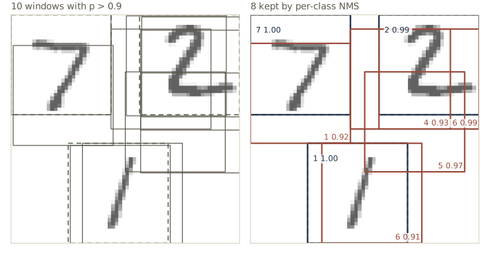
Two copies of the 64 by 64 scene with three handwritten digits. Left: all candidate windows with class probability above 0.9 drawn as thin rectangles labeled with their class. Right: the windows kept by per-class non-max suppression; correct detections are navy, wrong-class detections rust, and the true digit frames are dashed. — Left: every window of the sliding-window detector with a class probability above 0.9. Right: after per-class non-max suppression with IoU threshold 0.3. Navy boxes match a digit of the same class; rust boxes are confident mistakes on partial digits, which a background class in training would suppress. Dashed boxes: the true digit frames.

Fast region CNNs

A sliding window spends the full network on every part of the image, including large empty regions. Region-based detectors first propose a manageable set of regions likely to contain an object, using a cheaper method (originally a bottom-up segmentation algorithm), and then classify only those. Fast R-CNN (Girshick, 2015) makes this efficient by computing the convolutional feature maps once for the whole image, and then, for each proposed region, cutting out the matching part of the feature map and converting it to a fixed size with RoI pooling (region-of-interest pooling): the region is divided into a fixed grid of cells, say \(4 \times 4\), and each cell is max-pooled. Every region, whatever its size or shape, thus yields a feature tensor of the same shape, which the fully connected head classifies; a second head predicts corrections to the box. Faster R-CNN (Ren et al., 2015) replaces the external proposal method with a small region proposal network that runs on the same feature maps, so the whole detector is trained end to end. Predicting box offsets relative to a window or proposal is also how sliding-window detectors refine their coarse positions (Sermanet et al., 2013).

We write RoI max-pooling ourselves, following the conventions of torchvision.ops.roi_pool (the region’s corners are scaled to feature-map coordinates and rounded, and each cell covers the feature positions from the floor of its start to the ceiling of its end), and check it against the library. Then we do a small Fast R-CNN step with our trained network: one feature map for the whole scene, the three digit frames as region proposals, RoI pooling to the \(4 \times 4\) grid that fc1 expects, and the network’s own head as classifier.

The step that needs care is projecting an image box onto the feature map. The obvious projection multiplies coordinates by the total stride, here 1/2 for the last convolutional layer. But each unit of that layer sees a 14-pixel square (the receptive-field computation above), so unit \(p\) covers input pixels \(2p\) to \(2p + 13\), and the units lying entirely inside a frame that starts at pixel \(x_1\) and ends before \(x_2\) run from \(x_1/2\) to \((x_2 - 14)/2\). We try both.

def roi_max_pool(fmap, boxes, out_size, scale):
    """RoI max-pooling of a (C, H, W) feature map for boxes (R, 4) given in image coordinates."""
    Cf, H, W = fmap.shape
    out = torch.zeros(len(boxes), Cf, out_size, out_size)
    for r, (x1, y1, x2, y2) in enumerate(boxes.tolist()):
        xs, ys = round(x1 * scale), round(y1 * scale)
        width = max(round(x2 * scale) - xs + 1, 1)
        height = max(round(y2 * scale) - ys + 1, 1)
        for i in range(out_size):
            h0 = min(max(math.floor(i * height / out_size) + ys, 0), H)
            h1 = min(max(math.ceil((i + 1) * height / out_size) + ys, 0), H)
            for j in range(out_size):
                w0 = min(max(math.floor(j * width / out_size) + xs, 0), W)
                w1 = min(max(math.ceil((j + 1) * width / out_size) + xs, 0), W)
                if h1 > h0 and w1 > w0:                        # empty cells stay zero
                    out[r, :, i, j] = fmap[:, h0:h1, w0:w1].amax(dim=(1, 2))
    return out

with torch.no_grad():
    fmap = F.relu(cnn.features(scene))[0]                    # (16, 26, 26): computed once
    naive = roi_max_pool(fmap, true_boxes, 4, 0.5)           # corners times the stride
    ref = roi_pool(fmap[None], [true_boxes], output_size=(4, 4), spatial_scale=0.5)
    print("feature map", tuple(fmap.shape), "-> pooled regions", tuple(naive.shape))
    print(f"largest difference from torchvision roi_pool: {(naive - ref).abs().max().item():.1e}")
    fitted = torch.stack([true_boxes[:, 0] / 2, true_boxes[:, 1] / 2,
                          (true_boxes[:, 2] - 14) / 2, (true_boxes[:, 3] - 14) / 2], dim=1)
    exact = roi_max_pool(fmap, fitted, 4, 1.0)               # boxes already in feature coordinates
    for name, pooled in [("stride-scaled boxes", naive), ("receptive-field boxes", exact)]:
        logits = cnn.fc2(F.relu(cnn.fc1(pooled.flatten(1))))
        print(f"{name:22s}: classes {logits.argmax(1).tolist()}   (true {true_labels.tolist()})")
    frames = torch.stack([scene[0, :, r:r + 28, c:c + 28] for r, c in placements])
    print(f"receptive-field boxes vs classifying the cropped frames: largest logit difference "
          f"{(logits - cnn(frames)).abs().max().item():.1e}")

feature map (16, 26, 26) -> pooled regions (3, 16, 4, 4)
largest difference from torchvision roi_pool: 0.0e+00
stride-scaled boxes   : classes [7, 8, 6]   (true [7, 2, 1])
receptive-field boxes : classes [7, 2, 1]   (true [7, 2, 1])
receptive-field boxes vs classifying the cropped frames: largest logit difference 0.0e+00

With the stride-scaled boxes each region spans 15 feature cells instead of 8, so every pooling cell mixes in features from outside the digit, and the head, which never saw such inputs, gets two of the three digits wrong. With the boxes fitted to the receptive fields, RoI pooling of the shared map reproduces exactly what the network computes on each cropped frame. A real Fast R-CNN does not rely on such exact alignment: its head is trained on RoI-pooled features of many proposals of all shapes, so it learns to classify whatever the pooling produces. The shared feature map is computed once, and each extra region costs only a pooling and the small head. (The newer roi_align in torchvision replaces the rounding with bilinear interpolation, which gives more precise boxes.)

Image segmentation

Semantic segmentation assigns a class to every pixel. The output has the same spatial size as the input, with one channel per class holding that pixel’s class probabilities; coloring each pixel by its most probable class gives a label image. It is the most detailed of the three tasks: classification says what, detection says what and roughly where, segmentation says what is at each pixel.

Convolutional segmentation

A direct approach trains a classifier on a window centered on a pixel and applies it at every pixel (padding the image edges). As with detection, neighboring windows repeat almost all of their computation, and the fix is again to make the whole network convolutional. One could then keep every layer at full resolution, with stride 1, same padding, and no pooling, and put a softmax on each output pixel with weights shared across pixels. That works in principle, but a network deep and wide enough to recognize objects would then carry many channels at full resolution through every layer, which is far too expensive for images of useful size.

Up-sampling

The cure is the usual CNN pattern of down-sampling while adding channels, followed by the reverse: layers that bring the small, semantically rich maps back up to full resolution (Long, Shelhamer, and Darrell, 2015; Noh, Hong, and Han, 2015; Badrinarayanan, Kendall, and Cipolla, 2015). This encoder–decoder shape will return in the autoencoders of module 19, including masked autoencoders for images. We need operations that undo pooling and strided convolution.

The simplest is nearest-neighbor up-sampling: copy each value into all cells of its \(2 \times 2\) block. Average-pooling the result gives back the input exactly, so it is a right inverse of average pooling. For max-pooling, put each value in one cell of its block and zeros elsewhere, which max-pooling also inverts (for nonnegative values, as after a ReLU). Always using the first cell is arbitrary. Max-unpooling (as in SegNet, Badrinarayanan et al.) does better by remembering, in the down-sampling layer, which cell of each block held the maximum, and placing the value back there in the matching up-sampling layer. Bilinear up-sampling interpolates smoothly instead.

P2 = torch.tensor([[[[3., 1.], [0., 5.]]]])
near = F.interpolate(P2, scale_factor=2, mode="nearest")
print("nearest-neighbor copy:\n", near[0, 0].numpy(), "  average-pools back:", torch.equal(F.avg_pool2d(near, 2), P2))
first = torch.zeros(1, 1, 4, 4)
first[..., ::2, ::2] = P2
print("first cell of each block:\n", first[0, 0].numpy(), "  max-pools back:", torch.equal(F.max_pool2d(first, 2), P2))

pooled, where = F.max_pool2d(A4, 2, return_indices=True)       # A4 from the pooling section
unpooled = torch.zeros(1, 1, 16).scatter(2, where.flatten(2), pooled.flatten(2)).view(1, 1, 4, 4)
print("max-unpooling to the remembered positions:\n", unpooled[0, 0].numpy())
print("same as F.max_unpool2d:", torch.equal(unpooled, F.max_unpool2d(pooled, where, 2)),
      "  max-pools back:", torch.equal(F.max_pool2d(unpooled, 2), pooled))
print("bilinear:\n", F.interpolate(P2, scale_factor=2, mode="bilinear", align_corners=False)[0, 0].numpy())

nearest-neighbor copy:
 [[3. 3. 1. 1.]
 [3. 3. 1. 1.]
 [0. 0. 5. 5.]
 [0. 0. 5. 5.]]   average-pools back: True
first cell of each block:
 [[3. 0. 1. 0.]
 [0. 0. 0. 0.]
 [0. 0. 5. 0.]
 [0. 0. 0. 0.]]   max-pools back: True
max-unpooling to the remembered positions:
 [[0. 7. 0. 0.]
 [0. 0. 0. 8.]
 [0. 0. 0. 0.]
 [9. 0. 4. 0.]]
same as F.max_unpool2d: True   max-pools back: True
bilinear:
 [[3.     2.5    1.5    1.    ]
 [2.25   2.1875 2.0625 2.    ]
 [0.75   1.5625 3.1875 4.    ]
 [0.     1.25   3.75   5.    ]]

Fully convolutional networks

The up-sampling methods above are fixed, like pooling. A learned alternative mirrors strided convolution. In a strided convolution, each output unit collects a weighted patch of the input, and one step in the output moves the patch \(S\) steps in the input. Reverse the roles: each input unit spreads its value, times the kernel, over a patch of the output, and one step in the input moves the patch \(S\) steps in the output. Where patches overlap, the contributions are added. The output side length is

\[J_{\mathrm{out}} = (J - 1) S - 2P + M,\]

for input side \(J\), kernel \(M\), stride \(S\), and \(P\) rows and columns trimmed from each border (PyTorch’s padding), which inverts the size formula of a strided convolution.

The name transposed convolution comes from the matrix view. Write a strided convolution as \(\mathbf{y} = \mathbf{A}\mathbf{x}\), with \(\mathbf{A}\) the sparse, weight-sharing matrix we built earlier. The spreading operation just described is multiplication by \(\mathbf{A}^{\mathrm{T}}\): entry \(A_{pq}\) is the weight linking input \(q\) to output \(p\) in the convolution, and the transposed operation sends output \(p\)’s value back to input \(q\) with the same weight. Equivalently, it is the adjoint: \(\langle \mathbf{A}\mathbf{x}, \mathbf{z} \rangle = \langle \mathbf{x}, \mathbf{A}^{\mathrm{T}}\mathbf{z} \rangle\) for all \(\mathbf{x}, \mathbf{z}\). It is also the operation backpropagation performs to send errors from a convolution’s output to its input, which is how deep learning libraries implement it. Because the stride of a convolution is the ratio of input steps to output steps, the transposed version is also called a fractionally strided convolution (stride 1/2 for the figure’s case). Calling it a “deconvolution” is common but misleading: deconvolution in mathematics means inverting a convolution, and \(\mathbf{A}^{\mathrm{T}}\) is not \(\mathbf{A}^{-1}\).

We implement it with the spreading loop, check it against F.conv_transpose2d, and then verify that it is the transpose of the matrix of the matching strided convolution.

def conv_transpose2d(Z, W, stride=1, padding=0):
    """Each input unit adds its value times the kernel into the output; kernels land `stride` apart.

    Z: (N, C_in, H, W); W: (C_in, C_out, M, M) as in PyTorch. Output side (H - 1) S - 2P + M.
    """
    N, _, H, Wd = Z.shape
    M = W.shape[-1]
    out = torch.zeros(N, W.shape[1], (H - 1) * stride + M, (Wd - 1) * stride + M)
    for i in range(H):
        for j in range(Wd):
            out[:, :, i * stride:i * stride + M, j * stride:j * stride + M] += \
                torch.einsum("nc,cokl->nokl", Z[:, :, i, j], W)
    return out[:, :, padding:out.shape[2] - padding, padding:out.shape[3] - padding]

Zt = torch.from_numpy(rng.normal(size=(2, 3, 4, 5))).float()
Wt = torch.from_numpy(rng.normal(size=(3, 2, 3, 3))).float()
worst = max((conv_transpose2d(Zt, Wt, s, p) - F.conv_transpose2d(Zt, Wt, stride=s, padding=p)).abs().max().item()
            for s in [1, 2, 3] for p in [0, 1])
print(f"largest difference from F.conv_transpose2d over 6 settings: {worst:.1e}")

W1c = torch.from_numpy(rng.normal(size=(1, 1, 3, 3))).float()
down = lambda x: conv2d(x, W1c, stride=2, padding=1)                 # 7 x 7 -> 4 x 4
up = lambda z: conv_transpose2d(z, W1c, stride=2, padding=1)         # 4 x 4 -> 7 x 7
A_down = conv_matrix(down, (1, 1, 7, 7))                             # (16, 49)
A_up = conv_matrix(up, (1, 1, 4, 4))                                 # (49, 16)
xv = torch.from_numpy(rng.normal(size=(1, 1, 7, 7))).float()
zv = torch.from_numpy(rng.normal(size=(1, 1, 4, 4))).float()
print("matrix of the strided convolution", tuple(A_down.shape), "; of the transposed one", tuple(A_up.shape))
print("transposed convolution = A^T:", torch.allclose(A_up, A_down.T, atol=1e-6))
print(f"<A x, z> = {(down(xv) * zv).sum().item():.5f}    <x, A^T z> = {(xv * up(zv)).sum().item():.5f}")

largest difference from F.conv_transpose2d over 6 settings: 1.9e-06
matrix of the strided convolution (16, 49) ; of the transposed one (49, 16)
transposed convolution = A^T: True
<A x, z> = -3.64656    <x, A^T z> = -3.64656

Overlapping patches can leave a pattern. With a \(3 \times 3\) kernel and stride 2, some output cells receive one contribution, some two, and some four, so even a constant input produces a checkerboard:

counts = conv_transpose2d(torch.ones(1, 1, 4, 4), torch.ones(1, 1, 3, 3), stride=2)
print(counts[0, 0].int().numpy())

[[1 1 2 1 2 1 2 1 1]
 [1 1 2 1 2 1 2 1 1]
 [2 2 4 2 4 2 4 2 2]
 [1 1 2 1 2 1 2 1 1]
 [2 2 4 2 4 2 4 2 2]
 [1 1 2 1 2 1 2 1 1]
 [2 2 4 2 4 2 4 2 2]
 [1 1 2 1 2 1 2 1 1]
 [1 1 2 1 2 1 2 1 1]]

Learned kernels can compensate, but such checkerboard artifacts are common in images produced by transposed convolutions. Choosing a kernel size divisible by the stride (as in the U-net below, with \(M = S = 2\), where patches do not overlap at all), or replacing the transposed convolution by nearest-neighbor or bilinear up-sampling followed by an ordinary convolution, avoids them.

A network built only from convolutions (strided ones for down-sampling, transposed ones for up-sampling), with no fully connected layers, is a fully convolutional network (Long, Shelhamer, and Darrell, 2015). It accepts an image of any size and returns a label map of the matching size.

The U-net architecture

Down-sampling lets a network add channels and see large regions cheaply, but it discards precise positions, which is harmless for a class label and damaging for a per-pixel label. The U-net (Ronneberger, Fischer, and Brox, 2015) repairs this with skip connections. Its down-sampling path and up-sampling path mirror each other; drawn as a diagram they form a U. At each resolution, the last feature maps of the down-sampling path are copied across and concatenated, along the channel dimension, with the first feature maps of the up-sampling path at the same resolution. The decoder thus sees both the coarse “what” from below and the fine “where” from across. A final \(1 \times 1\) convolution maps the channels to \(K\) class scores per pixel, followed by a softmax, and the error is the cross-entropy summed over pixels,

\[E(\mathbf{w}) = -\sum_{n=1}^{N} \sum_{p} \sum_{k=1}^{K} t_{npk} \ln y_{k}(\mathbf{x}_n, p, \mathbf{w}),\]

where \(p\) runs over pixels and \(t_{npk}\) is 1 if pixel \(p\) of image \(n\) belongs to class \(k\). U-nets are also the standard denoising network inside the diffusion models of module 20.

Our data are synthetic: \(24 \times 24\) images containing a disc, a square, or both, with random sizes and positions, noisy intensities, and three pixel classes (background, disc, square). Telling a disc pixel from a square pixel needs context, since the interior of both shapes looks the same locally.

def make_shapes(n, rng, size=24, noise=0.2):
    """Images with up to one disc and one square; pixel labels 0 background, 1 disc, 2 square."""
    yy, xx = np.mgrid[0:size, 0:size]
    images = np.zeros((n, 1, size, size), np.float32)
    labels = np.zeros((n, size, size), np.int64)
    for i in range(n):
        for shape in rng.permutation(2):                     # random drawing order
            if rng.random() < 0.15:
                continue                                     # sometimes leave this shape out
            if shape == 0:
                r = rng.uniform(3, 7)
                cx, cy = rng.uniform(r, size - r, 2)
                mask = (xx - cx) ** 2 + (yy - cy) ** 2 <= r ** 2
            else:
                side = rng.integers(5, 13)
                x0, y0 = rng.integers(0, size - side, 2)
                mask = (xx >= x0) & (xx < x0 + side) & (yy >= y0) & (yy < y0 + side)
            labels[i][mask] = shape + 1
        images[i, 0] = (labels[i] > 0) * rng.uniform(0.5, 1.0)
    images += rng.normal(0, noise, images.shape).astype(np.float32)
    return torch.from_numpy(images), torch.from_numpy(labels)

rng_seg = np.random.default_rng(10)
X_seg, T_seg = make_shapes(1200, rng_seg)
X_seg_val, T_seg_val = make_shapes(300, rng_seg)
print("images", tuple(X_seg.shape), " labels", tuple(T_seg.shape))
print("pixel class frequencies:", np.bincount(T_seg.flatten().numpy()) / T_seg.numel())

images (1200, 1, 24, 24)  labels (1200, 24, 24)
pixel class frequencies: [0.7854 0.1126 0.1021]

The network has two levels of down-sampling (\(24 \to 12 \to 6\)), each level a pair of \(3 \times 3\) same convolutions with batch normalization and ReLU, \(2 \times 2\) transposed convolutions with stride 2 for up-sampling, and a skip connection at each of the two finer resolutions.

def double_conv(c_in, c_out):
    return nn.Sequential(nn.Conv2d(c_in, c_out, 3, padding=1), nn.BatchNorm2d(c_out), nn.ReLU(),
                         nn.Conv2d(c_out, c_out, 3, padding=1), nn.BatchNorm2d(c_out), nn.ReLU())

class UNet(nn.Module):
    def __init__(self, c=8, K=3):
        super().__init__()
        self.down1, self.down2 = double_conv(1, c), double_conv(c, 2 * c)
        self.bottom = double_conv(2 * c, 4 * c)
        self.up2, self.dec2 = nn.ConvTranspose2d(4 * c, 2 * c, 2, stride=2), double_conv(4 * c, 2 * c)
        self.up1, self.dec1 = nn.ConvTranspose2d(2 * c, c, 2, stride=2), double_conv(2 * c, c)
        self.out = nn.Conv2d(c, K, 1)                        # 1x1 convolution to K class scores

    def forward(self, x, trace=False):
        h1 = self.down1(x)                                   # full resolution
        h2 = self.down2(F.max_pool2d(h1, 2))                 # 1/2
        b = self.bottom(F.max_pool2d(h2, 2))                 # 1/4
        u2 = self.dec2(torch.cat([self.up2(b), h2], dim=1))  # skip connection at 1/2
        u1 = self.dec1(torch.cat([self.up1(u2), h1], dim=1)) # skip connection at full resolution
        if trace:
            for name, t in [("down 1", h1), ("down 2", h2), ("bottom", b), ("up 2 (after concat)", u2),
                            ("up 1 (after concat)", u1)]:
                print(f"  {name:20s} {tuple(t.shape)}")
        return self.out(u1)

torch.manual_seed(10)
unet = UNet()
print("output", tuple(unet(X_seg[:2], trace=True).shape), "  parameters",
      sum(p.numel() for p in unet.parameters()))

  down 1               (2, 8, 24, 24)
  down 2               (2, 16, 12, 12)
  bottom               (2, 32, 6, 6)
  up 2 (after concat)  (2, 16, 12, 12)
  up 1 (after concat)  (2, 8, 24, 24)
output (2, 3, 24, 24)   parameters 29659

Training uses Adam with a one-cycle learning-rate schedule (warm up, then decay) for five epochs. We report per-pixel accuracy and, for each class, the segmentation IoU: the number of pixels labeled that class in both the prediction and the truth, divided by the number labeled that class in either.

def seg_scores(logits, T, K=3):
    pred = logits.argmax(1)
    ious = [((pred == k) & (T == k)).sum().item() / max(((pred == k) | (T == k)).sum().item(), 1)
            for k in range(K)]
    return (pred == T).float().mean().item(), ious

epochs, batch = 5, 32
opt = torch.optim.Adam(unet.parameters(), lr=5e-3)
sched = torch.optim.lr_scheduler.OneCycleLR(opt, max_lr=5e-3, total_steps=epochs * math.ceil(1200 / batch))
gen = torch.Generator().manual_seed(0)
t0 = time.perf_counter()
for epoch in range(1, epochs + 1):
    unet.train()
    for idx in torch.randperm(len(X_seg), generator=gen).split(batch):
        loss = F.cross_entropy(unet(X_seg[idx]), T_seg[idx])    # mean over all pixels
        opt.zero_grad()
        loss.backward()
        opt.step()
        sched.step()
    unet.eval()
    with torch.no_grad():
        acc, ious = seg_scores(unet(X_seg_val), T_seg_val)
    print(f"epoch {epoch}  loss {loss.item():.3f}  pixel accuracy {acc:.4f}"
          f"  IoU background/disc/square {ious[0]:.3f} {ious[1]:.3f} {ious[2]:.3f}")
print(f"training time (your times will differ): {time.perf_counter() - t0:.1f} s")

epoch 1  loss 0.582  pixel accuracy 0.8431  IoU background/disc/square 0.931 0.399 0.024
epoch 2  loss 0.240  pixel accuracy 0.9091  IoU background/disc/square 0.986 0.535 0.202
epoch 3  loss 0.128  pixel accuracy 0.9748  IoU background/disc/square 0.994 0.801 0.804
epoch 4  loss 0.088  pixel accuracy 0.9797  IoU background/disc/square 0.996 0.832 0.842
epoch 5  loss 0.103  pixel accuracy 0.9806  IoU background/disc/square 0.996 0.840 0.847
training time (your times will differ): 11.5 s

For comparison, labeling every pixel as background would already give an accuracy of about 0.79, which is why the per-class IoU is the more telling number. After a couple of epochs of learning where the shapes are, the network learns to tell discs from squares, and it ends with an IoU well above 0.8 for both shapes. The remaining errors sit mostly on boundaries, where noise makes the edge ambiguous, and on small shapes.

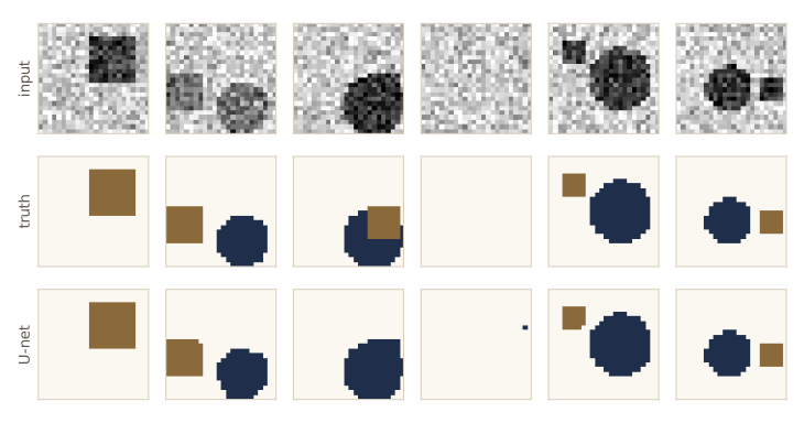
Validation images (top), true pixel labels (middle; navy = disc, brass = square), and the trained U-net's labels (bottom). The shapes are found almost exactly; mistakes are confined to a few boundary pixels, plus the third example, where a square drawn over a disc has the same intensity as the disc and is labeled disc.

In practice. Real segmentation data are much harder: classes are imbalanced (a small tumor in a large scan), and boundaries matter. Common remedies are class-weighted cross-entropy, losses based on overlap such as the Dice loss, heavy data augmentation, and larger U-nets with four or five levels. Everything in the network above stays the same in kind.

Style transfer

Early layers of a CNN respond to local, low-level structure (edges, colors, textures); later layers respond to larger arrangements and whole objects. Neural style transfer (Gatys, Ecker, and Bethge, 2015) uses this to redraw a content image \(\mathbf{C}\), say a photograph, in the style of another image \(\mathbf{S}\), say a painting. The generated image \(\mathbf{G}\) minimizes

\[E(\mathbf{G}) = E_{\mathrm{content}}(\mathbf{G}, \mathbf{C}) + E_{\mathrm{style}}(\mathbf{G}, \mathbf{S}),\]

starting from noise (or from \(\mathbf{C}\)), by gradient descent on the pixels of \(\mathbf{G}\), with the network’s weights fixed. What “content” and “style” mean is defined entirely by the two terms.

Content. Choose a convolutional layer and compare its pre-activations for the two images, position by position:

\[E_{\mathrm{content}}(\mathbf{G}, \mathbf{C}) = \sum_{i, j, k} \left\{ a_{ijk}(\mathbf{G}) - a_{ijk}(\mathbf{C}) \right\}^2 .\]

A deeper layer matches the arrangement of objects while leaving local detail free; an early layer holds \(\mathbf{G}\) close to the pixels of \(\mathbf{C}\).

Style. Style is about which features occur together, not where. If brushstrokes in one direction tend to come with a particular color in the painting, they should in the generated image too, anywhere in the frame. For one layer with \(K\) channels on an \(I \times J\) grid, the co-occurrence of channels \(k\) and \(k'\) is summed over all positions:

\[F_{kk'}(\mathbf{G}) = \sum_{i=1}^{I} \sum_{j=1}^{J} a_{ijk}(\mathbf{G})\, a_{ijk'}(\mathbf{G}).\]

If the layer’s activations are arranged as a \(K \times IJ\) matrix \(\mathbf{A}\), then \(\mathbf{F} = \mathbf{A}\mathbf{A}^{\mathrm{T}}\), the Gram matrix of the channels, also called the style matrix. The style error compares Gram matrices,

\[E_{\mathrm{style}}(\mathbf{G}, \mathbf{S}) = \frac{1}{(2IJK)^2} \sum_{k=1}^{K} \sum_{k'=1}^{K} \left\{ F_{kk'}(\mathbf{G}) - F_{kk'}(\mathbf{S}) \right\}^2 ,\]

and in practice it is summed over several layers with weights, \(\sum_l \lambda_l E^{(l)}_{\mathrm{style}}\), which captures texture at several scales. The weights, including the balance against the content term, are set by eye.

The key property of the Gram matrix is that it ignores position. Summing over \((i, j)\) means any rearrangement of the spatial positions, applied to all channels alike, leaves \(\mathbf{F}\) unchanged, while the content error changes a great deal:

def gram(A):
    """Style matrix F = A A^T for feature maps A of shape (K, I, J)."""
    Af = A.flatten(1)                                     # (K, IJ)
    return Af @ Af.T

with torch.no_grad():
    A_img = cnn.features(X_test[:1])[0]                   # (16, 8, 8) pre-activations
shuffle = torch.from_numpy(rng.permutation(64))
A_shuf = A_img.flatten(1)[:, shuffle].view_as(A_img)      # same spatial shuffle for every channel
print("Gram matrix", tuple(gram(A_img).shape), " max change after shuffling positions (round-off):",
      f"{(gram(A_shuf) - gram(A_img)).abs().max().item():.1e}")
print(f"content error between the two: {((A_shuf - A_img) ** 2).sum().item():.1f}"
      f"   (sum of squares of A itself: {(A_img ** 2).sum().item():.1f})")

Gram matrix (16, 16)  max change after shuffling positions (round-off): 1.2e-04
content error between the two: 12077.3   (sum of squares of A itself: 6525.2)

Note. Real style transfer uses a large network pretrained on natural images, typically VGG, whose features describe paintings and photographs well. Pretrained weights cannot be downloaded in the environment where these notes are run, and our MNIST network has only seen digits, so its “style” vocabulary is limited to stroke directions and thicknesses. With internet access, torchvision.models.vgg19(weights="DEFAULT").features gives the usual feature extractor, and the code below works unchanged with its layers.

To see the mechanics on a small scale, we use our trained LeNet as the feature extractor: content from the last convolutional layer, style from both convolutional layers. The content image is a test digit; the style image is a pattern of diagonal stripes. We start \(\mathbf{G}\) at the content image and run Adam on its pixels.

def conv_layers(x):
    """Pre-activations of the two convolutional layers of the trained LeNet."""
    a1 = cnn.conv1(x)
    a2 = cnn.conv2(F.max_pool2d(F.relu(a1), 2))
    return a1[0], a2[0]

def style_error(A, B):
    K, I, J = A.shape
    return ((gram(A) - gram(B)) ** 2).sum() / (2 * I * J * K) ** 2

yy, xx = torch.meshgrid(torch.arange(28.), torch.arange(28.), indexing="ij")
stripes = (0.5 + 0.5 * torch.sin(2 * math.pi * (xx + yy) / 7))[None, None]     # style image S
content = X_test[3:4]                                                          # content image C
for p in cnn.parameters():
    p.requires_grad_(False)                                   # the network stays fixed
with torch.no_grad():
    a_C = conv_layers(content)[1]
    S_feats = conv_layers(stripes)

G = content.clone().requires_grad_(True)
opt = torch.optim.Adam([G], lr=0.02)
beta = 1000.0                                                 # weight of the style term
for step in range(201):
    feats = conv_layers(G)
    E_content = ((feats[1] - a_C) ** 2).sum()
    E_style = sum(style_error(a, s) for a, s in zip(feats, S_feats))
    if step % 50 == 0:
        print(f"step {step:3d}:  E_content {E_content.item():8.2f}   E_style {E_style.item():8.4f}"
              f"   classified as {cnn(G).argmax().item()}")
    opt.zero_grad()
    (E_content + beta * E_style).backward()
    opt.step()
    with torch.no_grad():
        G.clamp_(0, 1)
for p in cnn.parameters():
    p.requires_grad_(True)
print(f"the content digit is a {y_test[3].item()}; for scale, the sum of squares of a(C) is {(a_C ** 2).sum().item():.0f}")

step   0:  E_content     0.00   E_style   6.9891   classified as 0
step  50:  E_content  1399.92   E_style   1.2324   classified as 0
step 100:  E_content  1336.27   E_style   1.2547   classified as 0
step 150:  E_content  1337.72   E_style   1.2368   classified as 0
step 200:  E_content  1336.63   E_style   1.2287   classified as 0
the content digit is a 0; for scale, the sum of squares of a(C) is 11433

Within 50 steps the style error falls to less than a fifth of its starting value and then levels off. The content error rises from zero to about an eighth of the size of the content features themselves, and the image is still read as the same digit: the optimizer keeps the features that define the digit in the last layer and fills the rest of the image with stroke fragments that reproduce the stripes’ channel co-occurrences. With a pretrained VGG network and photographs, the same loop, run for a few hundred steps at higher resolution with several style layers, produces the painterly results of the original paper.

Summary

Idea	What it does	Key formula or property
Convolutional layer	sparse, weight-shared feature detector	\(C(j, k) = \sum_l \sum_m I(j + l, k + m) K(l, m)\); equivariant to shifts
Padding and stride	control the output size	\(\lfloor (J + 2P - M)/S \rfloor + 1\); same padding \(P = (M - 1)/2\)
Channels	many features per position	\((M^2 C_{\mathrm{in}} + 1) C_{\mathrm{out}}\) parameters; 1 × 1 convolution mixes channels
Pooling	down-sampling, approximate invariance	max or average over windows; no parameters
Receptive field	region of the input a unit sees	\(r_l = r_{l-1} + (M_l - 1) j_{l-1}\), \(j_l = j_{l-1} S_l\)
Saliency, Grad-CAM	which pixels or regions drove a decision	\(\partial a^{(c)}/\partial \mathbf{x}\); \(L = \sum_k \alpha_k \mathbf{A}^{(k)}\)
FGSM	adversarial input	\(\mathbf{x}' = \mathbf{x} + \epsilon \operatorname{sign}(\nabla_{\mathbf{x}} E)\); effect grows with \(D\)
IoU and NMS	score boxes, remove duplicate detections	intersection / union; greedy keep-best, drop overlaps
Fully convolutional sliding window	classify every window in one pass	fully connected layers become convolutions
RoI pooling	fixed-size features for any region	max-pool a grid of cells in the shared feature map
Transposed convolution	learned up-sampling	multiplication by \(\mathbf{A}^{\mathrm{T}}\); side \((J - 1)S - 2P + M\)
U-net	per-pixel labels	encoder–decoder with skip concatenations at each resolution
Style transfer	content of one image, style of another	content: match activations; style: match Gram matrices \(\mathbf{A}\mathbf{A}^{\mathrm{T}}\)

Ideas to carry forward:

A convolution is a fully connected layer with a very particular sparsity and sharing pattern. That pattern is an inductive bias (locality plus translation equivariance), and it is why a CNN beats a fully connected network with four times its parameters on a few thousand digits.
Equivariance keeps track of where; pooling, striding, and global aggregation trade position for invariance. Classification wants invariance, detection and segmentation need position, and architectures such as fully convolutional networks and U-nets are ways of keeping both.
Gradients with respect to the input are as useful as gradients with respect to the weights: they give saliency maps, adversarial examples, synthetic images, DeepDream, and style transfer, all by the same backpropagation.
Many detection and segmentation tricks are about sharing computation: compute feature maps once and reuse them for every window or region.

Exercises

Show that true convolution, \(\sum_l \sum_m I(j - l, k - m) K(l, m)\), equals cross-correlation with the kernel rotated by 180 degrees, and state the ranges of \(l\) and \(m\) for a \(J \times K\) image and an \(L \times M\) kernel in both forms. Show that true convolution is commutative (\(I \ast K = K \ast I\) with suitable zero extension) while cross-correlation is not, and check both claims with scipy.signal.convolve2d and corr2d.
A kernel is separable if \(K(l, m) = f(l)\, g(m)\). Show that the 2-D cross-correlation with such a kernel equals a 1-D cross-correlation along columns with \(f\) followed by one along rows with \(g\), and count the multiply-adds per output pixel in both cases for an \(M \times M\) kernel. Verify that the Sobel filters are separable and implement the two-pass version.
Write down the \(5 \times 7\) matrix of a 1-D convolution with kernel \((w_1, w_2, w_3)\), stride 1, on seven inputs, and the \(3 \times 7\) matrix of the same convolution with stride 2 and no padding. Show by direct multiplication that the transpose of the second matrix, applied to \((z_1, z_2, z_3)\), gives the output of a transposed convolution with stride 2, and check with conv_matrix.
Derive the output size of a transposed convolution, \((J - 1)S - 2P + M\), from the spreading description, and show that feeding a strided convolution’s output size back into it recovers \(J\) exactly only when \((J + 2P - M)\) is divisible by \(S\). What does PyTorch’s output_padding argument do?
Count, for each of the 16 learnable layers of VGG-16, the number of parameters and the number of multiply-adds for one \(224 \times 224\) image. Which layer has the most parameters, and which does the most computation? Extend the counting cell of the notes to print both.
Train the LeNet on the pixel-shuffled images X_shuffled (apply the same permutation to the test images). Compare its accuracy with the unshuffled CNN and with the MLP trained on shuffled pixels. Explain the result in terms of the inductive bias of each network.
Add translation augmentation (random shifts of up to 3 pixels) to the training of the LeNet and measure the test accuracy on test digits shifted by 0 to 6 pixels, for the network with and without augmentation. How much invariance does the architecture alone provide, and how much does augmentation add?
Replace FGSM with its iterative version: take 10 steps of size \(\epsilon/4\), each followed by projection back onto the box \(\lVert \mathbf{x}' - \mathbf{x} \rVert_\infty \le \epsilon\) and onto \([0, 1]\). Plot accuracy against \(\epsilon\) for both attacks. Then train the LeNet on a mix of clean and FGSM images with \(\epsilon = 0.15\) and measure how its robustness to each attack changes.
Train a small network for single-object localization: place one digit at a random position on a \(40 \times 40\) canvas and predict its class (10 softmax outputs) and its ink box (4 linear outputs) with the error cross-entropy plus \(\lambda\) times the sum of squares. Report the classification accuracy and the fraction of test boxes with IoU above 0.5, and study the effect of \(\lambda\).
Train the U-net without its skip connections (the decoder sees only the up-sampled maps; adjust the channel counts) and compare the per-class IoU with the full U-net. Where in the images do the additional errors occur?
Show that the DeepDream objective \(F(I) = \sum_{ijk} a_{ijk}(I)^2\) has gradient \(\sum_{ijk} 2 a_{ijk} \nabla_I a_{ijk}\), and that for a linear layer \(\mathbf{a} = \mathbf{W}\mathbf{x}\) repeated normalized ascent steps turn \(\mathbf{x}\) toward the top right singular vector of \(\mathbf{W}\). What does this suggest DeepDream amplifies in a deep network?
In your own words: why does sharing one small kernel across all positions of an image help a network generalize from few examples, and what would it cost if images of your application had no translation symmetry (for example, a fixed-layout form where position carries meaning)?

Going further

Bishop & Bishop, Deep Learning: Foundations and Concepts, chapter 10 — the source for this module. Exercises 10.1 (feature detectors), 10.2–10.4 (convolution as a sparse matrix, cross-correlation vs convolution), 10.6–10.7 (padding and stride), 10.8 (VGG-16 parameters), 10.9 (separable kernels), 10.10 (DeepDream), 10.12 (convolutional sliding windows), and 10.13 (transposed convolution) extend the material here.
Vincent Dumoulin and Francesco Visin, “A guide to convolution arithmetic for deep learning”, arXiv:1603.07285 — pictures and formulas for every combination of padding, stride, and transposed convolution.
Yann LeCun, Léon Bottou, Yoshua Bengio, and Patrick Haffner, “Gradient-based learning applied to document recognition”, Proceedings of the IEEE, 1998 — LeNet and the case for convolutional networks.
Ian Goodfellow, Jonathon Shlens, and Christian Szegedy, “Explaining and harnessing adversarial examples”, arXiv:1412.6572 — the fast gradient sign method and the linear explanation.
Olaf Ronneberger, Philipp Fischer, and Thomas Brox, “U-Net: convolutional networks for biomedical image segmentation”, arXiv:1505.04597; and Leon Gatys, Alexander Ecker, and Matthias Bethge, “A neural algorithm of artistic style”, arXiv:1508.06576.
Related modules: invariance, equivariance, and residual connections in module 09; vision transformers in module 12; masked autoencoders in module 19; U-nets as denoisers in module 20; and the shorter treatment of invariances and convolutional networks in Intro to ML, module 05.

These notes follow the chapters of C. M. Bishop and H. Bishop, Deep Learning: Foundations and Concepts (Springer, 2024), the course text, which the authors make free to read online. The explanations, code, figures, and exercises here are written for this course; the book remains the reference, with the full derivations and many more exercises.