CSE 676 · Module 07 · Week 4
Gradient Descent
Error surfaces, batch and stochastic gradient descent, mini-batches and initialization, momentum, learning-rate schedules, RMSProp and Adam, and data, batch, and layer normalization.
Companion reading: Bishop & Bishop, Deep Learning: Foundations and Concepts, chapter 7, “Gradient Descent”
By the end of this module you can
- Classify the stationary points of an error function from the eigenvalues of its Hessian, and explain why a network’s error has many equivalent minima.
- Derive how batch gradient descent behaves on a quadratic error, including the stable range \(0 < \eta < 2/\lambda_{\max}\) and the dependence of the convergence rate on the condition number.
- Implement stochastic and mini-batch gradient descent, and measure how the gradient noise falls with the batch size.
- Derive Xavier and He initialization from variance propagation, and show what goes wrong in a deep tanh or ReLU stack without them.
- Implement momentum, Nesterov momentum, AdaGrad, RMSProp, and Adam in NumPy, explain why Adam needs its bias correction, and match
torch.optimstep for step. - Implement step, exponential, cosine, and warmup learning-rate schedules, and explain why stochastic gradient descent needs a decaying rate.
- Implement batch and layer normalization, including the running statistics batch normalization uses at inference, and match
torch.nn. - Compare plain SGD, momentum, and Adam when training a small network on MNIST.
Contents
- Error surfaces
- Gradient descent optimization
- Convergence
- Normalization
- Experiment: optimizers on MNIST
- Summary
- Exercises
- Going further
In module 06 we built deep networks: stacks of layers, each a linear map followed by a nonlinearity, with enough flexibility to represent almost any function we care about. A network is only useful once its weights and biases are set, and this module is about how we set them. As with the linear models of modules 04 and 05, we choose an error function \(E(\mathbf{w})\), usually the negative log likelihood of the training data, and look for a weight vector \(\mathbf{w}\) that makes it small.
For a network there is no formula for the minimizer, and probing \(E\) one value at a time is far too slow a way to search a space with millions of dimensions. Every practical training method uses the gradient \(\nabla E(\mathbf{w})\), the vector of partial derivatives of the error with respect to every weight. Module 08 shows how backpropagation computes it at a cost comparable to one forward pass. Here we take the gradient as given and ask how best to use it. One more point before we start: in deep learning the aim is not the exact minimum of the training error. What we want is a network that does well on new data, and the choice of optimizer, its step sizes, and when we stop all affect that, a theme module 09 takes up.
The module follows Bishop & Bishop chapter 7. We first look at the geometry of error surfaces and at what the Hessian says about a stationary point. Then we build the gradient descent family: batch, stochastic, and mini-batch updates, and how to initialize the weights so that a deep network can learn at all. Next come the methods that make gradient descent converge faster (momentum, learning-rate schedules, and the adaptive methods AdaGrad, RMSProp, and Adam), and finally normalization of the inputs and of the hidden layers. We write every optimizer and normalization layer ourselves in NumPy and check each against its PyTorch counterpart. The module ends by training the same small network on MNIST with three of our optimizers.
Error surfaces
Stationary points
Think of the error as a surface over weight space, the space of all weight vectors: each point \(\mathbf{w}\) has a height \(E(\mathbf{w})\). If we move from \(\mathbf{w}\) to \(\mathbf{w} + \delta\mathbf{w}\), the height changes by
\[\delta E \simeq \delta\mathbf{w}^{\mathrm{T}} \nabla E(\mathbf{w})\]to first order. Among all steps of a given small length, the one along \(\nabla E\) increases \(E\) fastest and the one along \(-\nabla E\) decreases it fastest. So as long as the gradient is not zero, a small step against it lowers the error. The places where we can stop are the stationary points, where
\[\nabla E(\mathbf{w}) = \mathbf{0}.\]A stationary point can be a minimum, a maximum, or a saddle point (downhill in some directions and uphill in others). A minimum whose error is the smallest over all of weight space is a global minimum; any other minimum is a local minimum.
To make this concrete we use a two-parameter error surface small enough to plot:
\[E(\mathbf{w}) = (w_1^2 - 1)^2 + (w_2^2 - 1)^2 + 0.3\, w_1 + 0.4\, w_1 w_2 .\]Without the last two terms it would have four minima at \((\pm 1, \pm 1)\); the tilt \(0.3\,w_1\) and the coupling \(0.4\,w_1 w_2\) make those minima unequal and rotate the curvature slightly. We find all its stationary points by running Newton’s method on the equation \(\nabla E = \mathbf{0}\) from a grid of starting points, keeping the distinct solutions.
import math
import numpy as np
import torch
import torch.nn.functional as F
from torchvision import datasets

np.set_printoptions(precision=4, suppress=True)
rng = np.random.default_rng(7)
torch.manual_seed(7)
def E_toy(w):
    """A two-parameter error surface with several stationary points."""
    w1, w2 = w
    return (w1**2 - 1)**2 + (w2**2 - 1)**2 + 0.3 * w1 + 0.4 * w1 * w2

def grad_toy(w):
    w1, w2 = w
    return np.array([4 * w1 * (w1**2 - 1) + 0.3 + 0.4 * w2,
                     4 * w2 * (w2**2 - 1) + 0.4 * w1])

def hess_toy(w):
    w1, w2 = w
    return np.array([[12 * w1**2 - 4, 0.4],
                     [0.4, 12 * w2**2 - 4]])

def newton(w, steps=50):
    """Newton's method for grad E = 0: w <- w - H^{-1} grad E."""
    for _ in range(steps):
        w = w - np.linalg.solve(hess_toy(w), grad_toy(w))
    return w

stationary = []
for a in np.linspace(-1.5, 1.5, 7):
    for b in np.linspace(-1.5, 1.5, 7):
        w = newton(np.array([a, b]))
        is_new = not any(np.allclose(w, s, atol=1e-6) for s in stationary)
        if np.linalg.norm(grad_toy(w)) < 1e-10 and is_new:
            stationary.append(w)
stationary.sort(key=E_toy)

print("     w1       w2        E     eigenvalues of H    type")
for w in stationary:
    lam = np.linalg.eigvalsh(hess_toy(w))
    kind = "minimum" if lam.min() > 0 else "maximum" if lam.max() < 0 else "saddle"
    print(f"{w[0]:7.4f}  {w[1]:7.4f}  {E_toy(w):7.4f}   {lam[0]:7.3f} {lam[1]:7.3f}"
          f"    {kind}")
     w1       w2        E     eigenvalues of H    type
-1.0801   1.0502  -0.7394     9.063  10.171    minimum
 1.0145  -1.0473  -0.1104     8.188   9.327    minimum
-0.9900  -0.9462   0.0891     6.606   7.901    minimum
 0.9006   0.9515   0.6576     5.606   6.991    minimum
-1.0308  -0.1042   0.7160    -3.882   8.764    saddle
-0.0249  -0.9988   1.0012    -4.006   7.983    saddle
 0.1799   0.9909   1.0619    -3.626   7.796    saddle
 0.9546   0.0964   1.3126    -3.903   6.951    saddle
 0.0762   0.0076   2.0114    -4.366  -3.563    maximum
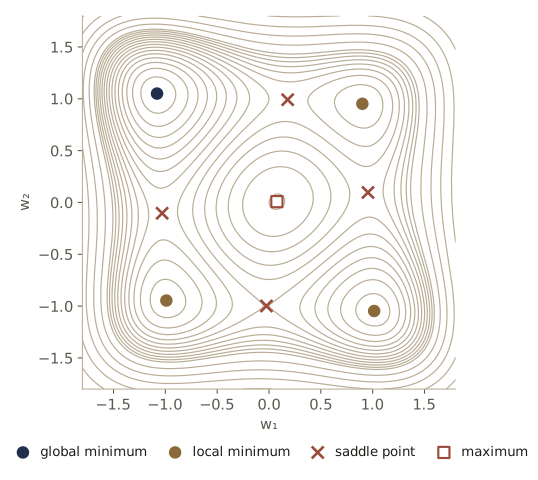
There are nine stationary points: four minima, four saddle points, and one maximum near the origin. The minimum at about \((-1.08, 1.05)\) is the global one; the other three are local minima with higher error. The last two columns already classify the points, and the next subsection explains why they can.
Local quadratic approximation
Near any point \(\widehat{\mathbf{w}}\) the error is well described by its second-order Taylor expansion,
\[E(\mathbf{w}) \simeq E(\widehat{\mathbf{w}}) + (\mathbf{w} - \widehat{\mathbf{w}})^{\mathrm{T}} \mathbf{b} + \frac12 (\mathbf{w} - \widehat{\mathbf{w}})^{\mathrm{T}} \mathbf{H} (\mathbf{w} - \widehat{\mathbf{w}}),\]where \(\mathbf{b} = \nabla E(\widehat{\mathbf{w}})\) is the gradient there and \(\mathbf{H}\) is the Hessian, the \(W \times W\) matrix of second derivatives \(H_{ij} = \partial^2 E / \partial w_i \partial w_j\) evaluated at \(\widehat{\mathbf{w}}\) (\(W\) is the total number of weights and biases). Differentiating the expansion gives the matching approximation of the gradient,
\[\nabla E(\mathbf{w}) \simeq \mathbf{b} + \mathbf{H} (\mathbf{w} - \widehat{\mathbf{w}}).\]Now expand around a stationary point \(\mathbf{w}^{\star}\). The linear term vanishes, and we are left with
\[E(\mathbf{w}) \simeq E(\mathbf{w}^{\star}) + \frac12 (\mathbf{w} - \mathbf{w}^{\star})^{\mathrm{T}} \mathbf{H} (\mathbf{w} - \mathbf{w}^{\star}).\]The Hessian is symmetric, so it has real eigenvalues \(\lambda_i\) and a complete set of orthonormal eigenvectors \(\mathbf{u}_i\):
\[\mathbf{H}\mathbf{u}_i = \lambda_i \mathbf{u}_i, \qquad \mathbf{u}_i^{\mathrm{T}}\mathbf{u}_j = \delta_{ij}.\]We use the eigenvectors as new coordinate axes centered on \(\mathbf{w}^{\star}\), writing \(\mathbf{w} - \mathbf{w}^{\star} = \sum_i \alpha_i \mathbf{u}_i\), so that \(\alpha_i = \mathbf{u}_i^{\mathrm{T}}(\mathbf{w} - \mathbf{w}^{\star})\) is the displacement along the \(i\)-th axis. Substituting and using the two properties of the eigenvectors,
\[(\mathbf{w} - \mathbf{w}^{\star})^{\mathrm{T}} \mathbf{H} (\mathbf{w} - \mathbf{w}^{\star}) = \sum_i \sum_j \alpha_i \alpha_j\, \mathbf{u}_i^{\mathrm{T}} \mathbf{H} \mathbf{u}_j = \sum_i \sum_j \alpha_i \alpha_j \lambda_j \delta_{ij} = \sum_i \lambda_i \alpha_i^2 ,\]and therefore
Result. Near a stationary point, in the coordinates of the Hessian’s eigenvectors, the error is a sum of independent one-dimensional parabolas:
\[E(\mathbf{w}) \simeq E(\mathbf{w}^{\star}) + \frac12 \sum_i \lambda_i \alpha_i^2 .\]
Moving along \(\mathbf{u}_j\) alone raises the error if \(\lambda_j > 0\) and lowers it if \(\lambda_j < 0\). So a stationary point is a minimum if all eigenvalues are positive, a maximum if all are negative, and a saddle point if there are some of each. “All eigenvalues positive” is the same as positive definiteness, \(\mathbf{v}^{\mathrm{T}}\mathbf{H}\mathbf{v} > 0\) for every nonzero \(\mathbf{v}\): writing \(\mathbf{v} = \sum_i c_i \mathbf{u}_i\) gives \(\mathbf{v}^{\mathrm{T}}\mathbf{H}\mathbf{v} = \sum_i \lambda_i c_i^2\), which is positive for every nonzero \(\mathbf{c}\) exactly when every \(\lambda_i > 0\). Near a minimum, the contours of constant error are ellipsoids with axes along the \(\mathbf{u}_i\); setting \(\tfrac12 \lambda_i \alpha_i^2 = c\) shows that the semi-axis along \(\mathbf{u}_i\) has length \(\sqrt{2c/\lambda_i}\), so strongly curved directions give short axes and weakly curved ones long axes. If an eigenvalue is zero, the quadratic approximation is flat in that direction and higher-order terms decide.
We can check the expansion numerically. Starting at the global minimum of the toy surface, we step a distance \(r\) along a fixed direction and compare the true rise in error with \(\tfrac12 \sum_i \lambda_i \alpha_i^2\).
w_star = stationary[0]                        # the global minimum
H_star = hess_toy(w_star)
lam, U = np.linalg.eigh(H_star)               # H u_i = lambda_i u_i; U has columns u_i
d = np.array([0.6, -0.8])                     # a unit direction in weight space

print("   r    E(w) - E(w*)   (1/2) sum lambda_i alpha_i^2   difference")
for r in [0.3, 0.1, 0.03, 0.01]:
    w = w_star + r * d
    alpha = U.T @ (w - w_star)                # alpha_i = u_i^T (w - w*)
    quadratic = 0.5 * np.sum(lam * alpha**2)
    exact = E_toy(w) - E_toy(w_star)
    print(f"{r:5.2f}   {exact:.6e}   {quadratic:.6e}"
          f"                 {exact - quadratic:9.2e}")
   r    E(w) - E(w*)   (1/2) sum lambda_i alpha_i^2   difference
 0.30   3.317655e-01   4.106651e-01                 -7.89e-02
 0.10   4.259941e-02   4.562946e-02                 -3.03e-03
 0.03   4.023821e-03   4.106651e-03                 -8.28e-05
 0.01   4.532160e-04   4.562946e-04                 -3.08e-06
Each time \(r\) shrinks by a factor of about three, the discrepancy shrinks by roughly the cube of that factor: it is a cubic effect, the first term the expansion leaves out. Close to a minimum, the quadratic picture is accurate, and most of what follows about convergence speed is derived from it. The same local expansion, with ways to compute or approximate \(\mathbf{H}\) for a network, is developed in Intro to ML, module 05.
Why the error has many equivalent minima
For a neural network the error surface is far more complicated than our toy, and one reason is built in. Module 06 showed that many different weight vectors compute the same function. In a layer of \(M\) tanh hidden units we can relabel the units in \(M!\) ways, and flip the signs of the weights into and out of any unit, a further factor of \(2^M\). Every minimum is therefore one of at least \(M!\,2^M\) equivalent minima with exactly the same error, and the factors multiply across layers.
For ReLU units the sign flip does not work (ReLU is not odd), but a different symmetry does: since \(\mathrm{ReLU}(c\,a) = c\,\mathrm{ReLU}(a)\) for \(c > 0\), we can multiply the weights and bias into a unit by \(c\) and divide the weights out of it by \(c\). This is a continuous family, so every minimum of a ReLU network lies on a curve (in fact an \(M\)-dimensional surface) of points with equal error, and along those directions the Hessian has zero eigenvalues. The next cell checks both symmetries for a small ReLU network and counts the relabelings for the 128-unit hidden layer we train at the end of the module.
def relu_net(x, W1, b1, W2, b2):
    return np.maximum(W1 @ x + b1, 0) @ W2.T + b2

D_in, M_h, K_out = 3, 5, 2
W1, b1 = rng.normal(size=(M_h, D_in)), rng.normal(size=M_h)
W2, b2 = rng.normal(size=(K_out, M_h)), rng.normal(size=K_out)
x = rng.normal(size=D_in)

perm = rng.permutation(M_h)                  # relabel the hidden units
c = rng.uniform(0.2, 5.0, size=M_h)          # a positive scale per hidden unit
same_perm = relu_net(x, W1[perm], b1[perm], W2[:, perm], b2)
same_scale = relu_net(x, c[:, None] * W1, c * b1, W2 / c, b2)
print("outputs:", relu_net(x, W1, b1, W2, b2))
print("after relabeling:", same_perm, "  after rescaling:", same_scale)

M = 128
print(f"relabelings of {M} hidden units: M! = 10^{math.lgamma(M + 1) / math.log(10):.1f}")
outputs: [-1.8278 -0.508 ]
after relabeling: [-1.8278 -0.508 ]   after rescaling: [-1.8278 -0.508 ]
relabelings of 128 hidden units: M! = 10^215.6
These symmetries are harmless: all the equivalent minima are equally good, so it does not matter which one we land in. The harder question is whether there are poor, non-equivalent local minima that trap gradient descent. For small networks there can be. For large networks, experience says it is rarely a problem: training from different random starting points usually reaches solutions of similar quality. A heuristic argument points the same way. At a stationary point of a function of \(W\) variables, a minimum needs all \(W\) Hessian eigenvalues to be positive, which becomes a demanding condition when \(W\) is in the millions. Most stationary points at high error are then expected to be saddle points, which gradient descent can leave, rather than minima.
Gradient descent optimization
Solving \(\nabla E(\mathbf{w}) = \mathbf{0}\) in closed form is hopeless for a network, so we iterate. Starting from an initial vector \(\mathbf{w}^{(0)}\), every method we meet takes steps
\[\mathbf{w}^{(\tau)} = \mathbf{w}^{(\tau - 1)} + \Delta\mathbf{w}^{(\tau - 1)},\]where \(\tau\) counts iterations and the methods differ in how they choose the update \(\Delta\mathbf{w}\). On a nonconvex surface the answer depends on where we start, so it can pay to train from several random starting points and keep the network that does best on a validation set.
Use of gradient information
Why insist on gradients? The quadratic approximation gives a way to count. Near a minimum, the error surface is described by \(\mathbf{b}\) (\(W\) numbers) and the symmetric matrix \(\mathbf{H}\) (\(W(W+1)/2\) numbers), a total of \(W(W+3)/2\) unknowns. We cannot expect to pin down the minimum before we have gathered about that many independent pieces of information, which is \(O(W^2)\).
If all we can do is evaluate \(E\), each evaluation delivers one number and costs \(O(W)\) operations (every weight takes part in a forward pass), so the search costs \(O(W^2) \times O(W) = O(W^3)\). A gradient evaluation delivers \(W\) numbers at once. With backpropagation it costs only \(O(W)\), so about \(W\) gradient evaluations suffice and the total cost drops to \(O(W^2)\). For a network with a million weights, that factor of \(W\) separates the practical from the impossible.
We can watch the counting argument work on an exact quadratic. With values alone, we fit all \(1 + W + W(W+1)/2\) coefficients of a quadratic by solving a linear system built from that many function values. With gradients, the difference \(\nabla E(\mathbf{w}_0 + \mathbf{e}_i) - \nabla E(\mathbf{w}_0)\) is the \(i\)-th column of \(\mathbf{H}\), so \(W + 1\) gradient evaluations give \(\mathbf{H}\) and \(\mathbf{b}\), and one Newton step gives the minimum.
W_q = 6
A_q = rng.normal(size=(W_q, W_q))
H_q = A_q @ A_q.T + np.eye(W_q)                       # a positive definite Hessian
w_q_star = rng.normal(size=W_q)
E_q = lambda w: 0.5 * (w - w_q_star) @ H_q @ (w - w_q_star) + 1.0
grad_q = lambda w: H_q @ (w - w_q_star)

# (a) function values only: E = c + b^T w + (1/2) w^T H w has 1 + W + W(W+1)/2 unknowns
iu = np.triu_indices(W_q)
def quad_features(w):
    outer = np.outer(w, w)
    return np.concatenate([[1.0], w, np.where(iu[0] == iu[1], 0.5, 1.0) * outer[iu]])

n_values = 1 + W_q + W_q * (W_q + 1) // 2
W_samples = rng.normal(size=(n_values, W_q))
coef = np.linalg.solve(np.array([quad_features(w) for w in W_samples]),
                       np.array([E_q(w) for w in W_samples]))
H_fit = np.zeros((W_q, W_q))
H_fit[iu] = coef[1 + W_q:]
H_fit = H_fit + H_fit.T - np.diag(np.diag(H_fit))
w_from_values = np.linalg.solve(H_fit, -coef[1:1 + W_q])

# (b) gradients: columns of H from gradient differences, then one Newton step
w0 = np.zeros(W_q)
g0 = grad_q(w0)
H_diff = np.column_stack([grad_q(w0 + e) - g0 for e in np.eye(W_q)])
w_from_grads = w0 - np.linalg.solve(H_diff, g0)

err_values = np.abs(w_from_values - w_q_star).max()
err_grads = np.abs(w_from_grads - w_q_star).max()
print(f"{n_values} function values:     max error in w* = {err_values:.1e}")
print(f"{W_q + 1} gradient evaluations: max error in w* = {err_grads:.1e}")
28 function values:     max error in w* = 8.8e-15
7 gradient evaluations: max error in w* = 3.9e-16
Both recover the minimum to rounding error, but values alone needed four times as many evaluations even at \(W = 6\), and the gap grows like \(W/2\). Real error functions are not quadratic, so no method finishes in a fixed number of steps, but the advantage of gradients carries over.
Batch gradient descent
The simplest way to use the gradient is to step against it:
\[\mathbf{w}^{(\tau)} = \mathbf{w}^{(\tau - 1)} - \eta \nabla E(\mathbf{w}^{(\tau - 1)}),\]where \(\eta > 0\) is the learning rate. This is gradient descent, also called steepest descent. When \(E\) is defined over the whole training set, every step processes all of the data; methods that do this are called batch methods.
How fast does it converge, and how large may \(\eta\) be? Near a minimum we can answer exactly with the quadratic approximation. There \(\nabla E = \mathbf{H}(\mathbf{w} - \mathbf{w}^{\star}) = \sum_i \lambda_i \alpha_i \mathbf{u}_i\). Writing the update as \(\Delta\mathbf{w} = \sum_i \Delta\alpha_i \mathbf{u}_i\) and taking the inner product of the update equation with \(\mathbf{u}_i\) gives
\[\Delta\alpha_i = -\eta \lambda_i \alpha_i, \qquad \text{so} \qquad \alpha_i^{(\tau)} = (1 - \eta\lambda_i)\, \alpha_i^{(\tau - 1)} = (1 - \eta\lambda_i)^{\tau} \alpha_i^{(0)} .\]Each eigendirection evolves on its own, shrinking by the factor \(1 - \eta\lambda_i\) at every step. The iteration converges to \(\mathbf{w}^{\star}\) when all these factors have magnitude below one, \(-1 < 1 - \eta\lambda_i < 1\). The right inequality holds whenever \(\eta\lambda_i > 0\), which requires the stationary point to be a minimum; the left one requires \(\eta\lambda_i < 2\) for every \(i\).
Result. On a quadratic error with Hessian eigenvalues \(0 < \lambda_{\min} \le \dots \le \lambda_{\max}\), gradient descent converges if and only if
\[0 < \eta < \frac{2}{\lambda_{\max}} .\]The distance to the minimum then shrinks at least by the factor \(\max_i \lvert 1 - \eta\lambda_i \rvert\) per step, which is at best \((\kappa - 1)/(\kappa + 1)\), reached at \(\eta = 2/(\lambda_{\min} + \lambda_{\max})\). Here \(\kappa = \lambda_{\max}/\lambda_{\min}\) is the condition number of the Hessian.
The best rate comes from balancing the two extreme directions. The factor \(\lvert 1 - \eta\lambda_i \rvert\) is largest either at \(\lambda_{\min}\) (where \(1 - \eta\lambda_{\min}\) is close to one) or at \(\lambda_{\max}\) (where \(1 - \eta\lambda_{\max}\) may be close to \(-1\)). Increasing \(\eta\) helps the first and hurts the second, so the best \(\eta\) makes them equal, \(1 - \eta\lambda_{\min} = \eta\lambda_{\max} - 1\), which gives \(\eta = 2/(\lambda_{\min} + \lambda_{\max})\) and the factor \((\lambda_{\max} - \lambda_{\min})/(\lambda_{\max} + \lambda_{\min}) = (\kappa - 1)/(\kappa + 1)\). For large \(\kappa\) this is about \(1 - 2/\kappa\), so reducing the distance by a factor \(\epsilon\) takes about \((\kappa/2)\ln(1/\epsilon)\) steps. Gradient descent converges linearly (the error falls geometrically, by a constant factor per step), but the constant can be painfully close to one: the steep directions cap the learning rate, and the shallow directions then crawl.
Let us check this on a 20-dimensional quadratic whose Hessian has eigenvalues spread geometrically from 1 to \(\kappa\), with random eigenvectors. For the two learning rates \(\eta = 1/\lambda_{\max}\) and \(\eta = 2/(\lambda_{\min} + \lambda_{\max})\) we count the steps needed to reduce \(\lVert \mathbf{w} - \mathbf{w}^{\star} \rVert\) by a factor of \(10^6\), and compare with the prediction \(\ln(10^6)/(-\ln \rho)\) for the per-step factor \(\rho\).
def make_quadratic(eigs, rng):
    """Hessian with the given eigenvalues and random orthonormal eigenvectors; a minimum w*."""
    U, _ = np.linalg.qr(rng.normal(size=(len(eigs), len(eigs))))
    return U @ np.diag(eigs) @ U.T, rng.normal(size=len(eigs))

def gd_steps(H, w_star, eta, tol=1e-6, max_steps=100_000):
    """Batch gradient descent from w = 0 on E = (w - w*)^T H (w - w*) / 2.
    Returns the number of steps until ||w - w*|| < tol ||w*||."""
    w = np.zeros_like(w_star)
    for tau in range(1, max_steps + 1):
        w = w - eta * H @ (w - w_star)                    # w <- w - eta grad E
        if np.linalg.norm(w - w_star) < tol * np.linalg.norm(w_star):
            return tau
    return max_steps

print("kappa   1/lam_max: steps (predicted)   2/(lam_min+lam_max): steps (predicted)")
for kappa in [10, 100, 1000]:
    H_k, w_k = make_quadratic(np.geomspace(1, kappa, 20), rng)
    lo, hi = 1.0, float(kappa)
    pred_1 = np.log(1e6) / -np.log(1 - lo / hi)
    pred_2 = np.log(1e6) / -np.log((kappa - 1) / (kappa + 1))
    print(f"{kappa:5d}   {gd_steps(H_k, w_k, 1 / hi):18d} ({pred_1:6.0f})"
          f"   {gd_steps(H_k, w_k, 2 / (lo + hi)):24d} ({pred_2:6.0f})")

H_1000, w_1000 = H_k, w_k                                 # keep the kappa = 1000 problem
w = np.zeros(20)
for tau in range(200):
    w = w - (2.02 / 1000) * H_1000 @ (w - w_1000)         # just above the limit 2 / lam_max
print(f"eta = 2.02/lam_max: distance {np.linalg.norm(w_1000):.2f} at the start,"
      f" {np.linalg.norm(w - w_1000):.2f} after 200 steps")
kappa   1/lam_max: steps (predicted)   2/(lam_min+lam_max): steps (predicted)
   10                  121 (   131)                         66 (    69)
  100                 1108 (  1375)                        564 (   691)
 1000                12473 ( 13809)                       6363 (  6908)
eta = 2.02/lam_max: distance 5.22 at the start, 57.45 after 200 steps
The step counts follow the predictions (they come in somewhat under, because the starting point does not put all of its distance along the slowest eigenvector), and they grow in proportion to \(\kappa\): each tenfold increase in the condition number costs about ten times as many steps. The optimal learning rate saves a factor of two over \(\eta = 1/\lambda_{\max}\), no more. And a learning rate only 1% above the limit makes the steepest component grow by 2% per step: the iterates first settle along the other directions and then drift away, and the growth compounds without limit. The Hessian of a real network has eigenvalues spread over many orders of magnitude, so this picture, one steep direction limiting progress along all the others, is the main reason plain gradient descent is slow.
Stochastic gradient descent
The error functions we get from maximum likelihood with independent data points are sums over the data,
\[E(\mathbf{w}) = \sum_{n=1}^{N} E_n(\mathbf{w}),\]and computing the full gradient costs a pass over all \(N\) points. When \(N\) is in the millions, a single batch step is expensive, and it seems wasteful to look at every example before moving at all. Stochastic gradient descent (SGD) instead updates after each data point,
\[\mathbf{w}^{(\tau)} = \mathbf{w}^{(\tau - 1)} - \eta \nabla E_n(\mathbf{w}^{(\tau - 1)}),\]cycling through the data (in random order, as we will see). One complete pass through the training set is an epoch. When the data arrive as a stream and each point is used once, the same method is called online gradient descent.
Each single-point gradient is a noisy estimate of the full one. If we pick \(n\) uniformly at random, \(N\,\nabla E_n\) is an unbiased estimate of \(\nabla E\), so on average SGD moves downhill, and it makes \(N\) moves in the time batch gradient descent makes one. There are two further advantages. First, real data sets are redundant. If we duplicated every point, the error would double and a batch step would cost twice as much while pointing in the same direction; SGD would not notice any difference. Second, a stationary point of the total error is generally not a stationary point of each \(E_n\), so the noise can carry the weights past a shallow local minimum or off a saddle.
In code we will work with the mean error \(\frac{1}{N}\sum_n E_n\) rather than the sum. It has the same minimizer and just rescales \(\eta\) by \(N\), but it keeps good learning rates independent of the data set size, and it is what PyTorch’s losses compute by default. Here is a linear regression problem with \(N = 2000\) points and \(D = 10\) inputs. The inputs are correlated, as real features usually are (their covariance matrix has eigenvalues from 0.02 to 2), which gives the Hessian a condition number of about 100. We train it for five epochs with batch gradient descent (five steps at \(\eta = 1/\lambda_{\max}\)) and with SGD (10,000 single-point steps).
N, D = 2000, 10
Q_reg, _ = np.linalg.qr(rng.normal(size=(D, D)))
cov_half = Q_reg @ np.diag(np.sqrt(np.geomspace(0.02, 2, D))) @ Q_reg.T
X_reg = rng.normal(size=(N, D)) @ cov_half          # correlated inputs
t_reg = X_reg @ rng.normal(size=D) + 0.5 * rng.normal(size=N)
Phi = np.column_stack([np.ones(N), X_reg])        # a column of ones for the bias w_0

def E_reg(w):
    return 0.5 * np.mean((Phi @ w - t_reg) ** 2)

def grad_reg(w, idx=None):
    """Gradient of the mean error over the rows idx (all rows if idx is None)."""
    P, t = (Phi, t_reg) if idx is None else (Phi[idx], t_reg[idx])
    return P.T @ (P @ w - t) / len(t)

w_ls = np.linalg.lstsq(Phi, t_reg, rcond=None)[0]
E_min = E_reg(w_ls)
eta_batch = 1 / np.linalg.eigvalsh(Phi.T @ Phi / N)[-1]

w_batch, w_sgd = np.zeros(D + 1), np.zeros(D + 1)
rng_sgd = np.random.default_rng(1)
print(f"E_min = {E_min:.4f}")
print("epoch   batch GD: E - E_min   SGD (eta = 0.01): E - E_min")
for epoch in range(1, 6):
    w_batch -= eta_batch * grad_reg(w_batch)          # one batch step = one pass
    for n in rng_sgd.permutation(N):                  # N single-point steps = one pass
        w_sgd -= 0.01 * grad_reg(w_sgd, [n])
    print(f"{epoch:5d}   {E_reg(w_batch) - E_min:19.4f}   {E_reg(w_sgd) - E_min:23.5f}")

epochs = 5
while E_reg(w_batch) - E_min > 1e-3:                  # keep going with batch steps
    w_batch -= eta_batch * grad_reg(w_batch)
    epochs += 1
lam_reg = np.linalg.eigvalsh(Phi.T @ Phi / N)
print(f"condition number {lam_reg[-1] / lam_reg[0]:.0f}; batch GD reaches E - E_min < 1e-3 "
      f"after {epochs} epochs")
E_min = 0.1242
epoch   batch GD: E - E_min   SGD (eta = 0.01): E - E_min
    1                0.4700                   0.01579
    2                0.3057                   0.00669
    3                0.2394                   0.00366
    4                0.2005                   0.00455
    5                0.1724                   0.00126
condition number 105; batch GD reaches E - E_min < 1e-3 after 123 epochs
For the same number of passes over the data, SGD is within 0.016 of the minimum after the first epoch, while batch gradient descent, limited by the condition number of about 100, is still far away after five epochs and needs 123 to get within \(10^{-3}\). Notice, though, that SGD’s error does not keep falling: it hovers a small distance above the minimum, going up as well as down from epoch to epoch, because each step follows a noisy gradient with a fixed step size. We return to that floor when we discuss learning-rate schedules.
Mini-batches
Between one point and all of them lies the mini-batch: a small random subset of \(B\) points whose average gradient we use for each step. How much does averaging help? Let \(\mathbf{g}_n = \nabla E_n(\mathbf{w})\) be the per-point gradients and \(\bar{\mathbf{g}}\) their mean. For a mini-batch of \(B\) points drawn independently, the mini-batch gradient \(\mathbf{g}_B\) has mean \(\bar{\mathbf{g}}\) and
\[\mathbb{E}\left[ \lVert \mathbf{g}_B - \bar{\mathbf{g}} \rVert^2 \right] = \frac{1}{B} \cdot \frac{1}{N}\sum_{n=1}^{N} \lVert \mathbf{g}_n - \bar{\mathbf{g}} \rVert^2 ,\]the familiar fact that the variance of a mean of \(B\) independent terms is the single-term variance divided by \(B\). The typical error, the square root, therefore falls only like \(1/\sqrt{B}\): a batch 100 times larger gives a gradient only 10 times more accurate, at 100 times the cost. When the \(B\) points are drawn without replacement from a finite set of \(N\), the formula picks up a factor \((N - B)/(N - 1)\), which reaches zero when \(B = N\).
We measure this on the regression problem at \(\mathbf{w} = \mathbf{0}\), drawing 1000 mini-batches for each batch size.
def per_example_grads(w):
    """Row n is the gradient of E_n = (w^T phi_n - t_n)^2 / 2."""
    return Phi * (Phi @ w - t_reg)[:, None]

G = per_example_grads(np.zeros(D + 1))
g_bar = G.mean(axis=0)
single_var = np.mean(np.sum((G - g_bar) ** 2, axis=1))  # (1/N) sum_n ||g_n - g_bar||^2

rng_mb = np.random.default_rng(2)
batch_sizes = 2 ** np.arange(0, 11)
noise = []
print("    B   measured E||g_B - g||^2   predicted   relative size ||g_B - g|| / ||g||")
for B in batch_sizes:
    draws = [G[rng_mb.choice(N, B, replace=False)].mean(axis=0) for _ in range(1000)]
    measured = np.mean(np.sum((np.array(draws) - g_bar) ** 2, axis=1))
    predicted = single_var / B * (N - B) / (N - 1)
    noise.append(measured)
    relative = np.sqrt(measured) / np.linalg.norm(g_bar)
    print(f"{B:5d}   {measured:21.4f}   {predicted:9.4f}   {relative:19.3f}")
    B   measured E||g_B - g||^2   predicted   relative size ||g_B - g|| / ||g||
    1                 20.3213     18.3600                 3.042
    2                  9.4615      9.1754                 2.075
    4                  4.3867      4.5831                 1.413
    8                  2.1692      2.2870                 0.994
   16                  1.1195      1.1389                 0.714
   32                  0.5730      0.5649                 0.511
   64                  0.2757      0.2778                 0.354
  128                  0.1351      0.1343                 0.248
  256                  0.0621      0.0626                 0.168
  512                  0.0251      0.0267                 0.107
 1024                  0.0088      0.0088                 0.063
The measured noise tracks the prediction across three orders of magnitude, and it falls a little faster than \(1/B\) at the largest batch sizes, where \(B\) is a sizable fraction of \(N\). With a single point, the gradient error is about three times the size of the gradient itself; at eight points the two are about equal, and at 64 points the error is about a third of the gradient.
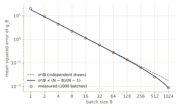
Which batch size to use is then mostly a question of hardware. On a GPU, a batch of 64 or 256 costs little more time than a batch of 1, because the points are processed in parallel, so the extra accuracy is nearly free up to the point where the device is fully used; sizes that are powers of two often map well onto the hardware. Beyond that, doubling \(B\) doubles the cost of a step but only reduces the noise by a factor of \(\sqrt{2}\).
The points in a mini-batch should be a random sample. Raw data sets are often ordered (by class, by date, by source), and batches of consecutive points would then give systematically biased gradients. The standard recipe shuffles the whole data set, takes consecutive blocks of \(B\) as mini-batches, and reshuffles at the start of every epoch, so that the batches differ from epoch to epoch.
Definition. Mini-batch stochastic gradient descent: repeat for each epoch: shuffle the indices \(1, \dots, N\); split them into consecutive blocks of \(B\); for each block \(\mathcal{B}\), update \(\mathbf{w} \leftarrow \mathbf{w} - \eta \nabla E_{\mathcal{B}}(\mathbf{w})\), where \(E_{\mathcal{B}} = \frac{1}{B}\sum_{n \in \mathcal{B}} E_n\). The name “stochastic gradient descent” is used for this whole family, whatever the batch size.
In code, the recipe is a generator that yields the index blocks of one epoch. We use it for the rest of the module.
def minibatches(N, B, rng):
    """Indices of one epoch of mini-batches: shuffle, then consecutive blocks of size B."""
    perm = rng.permutation(N)
    for start in range(0, N, B):
        yield perm[start:start + B]

print([len(idx) for idx in minibatches(N, 300, np.random.default_rng(0))])
[300, 300, 300, 300, 300, 300, 200]
The last block is shorter when \(B\) does not divide \(N\); some code drops it instead, which PyTorch’s DataLoader does when drop_last=True.
Parameter initialization
Gradient descent needs a starting point \(\mathbf{w}^{(0)}\), and for deep networks the choice matters a great deal: it affects how fast training goes, whether it gets going at all, and the quality of the network we end with. There is not much theory to guide it, but two principles are well established.
The first is symmetry breaking. If two hidden units in the same layer receive the same inputs and start with identical incoming and outgoing weights, they compute the same function, receive identical gradients, and therefore stay identical forever; the layer effectively has one unit. Initializing with all weights equal (for example all zero) wastes the whole layer. Random initial weights break the symmetry. We can watch this in a two-layer tanh network trained on a small nonlinear regression problem. PyTorch’s autograd supplies the gradients here; module 08 opens that box.
X_s = torch.from_numpy(rng.uniform(-2, 2, size=(200, 2)))
t_s = torch.sin(X_s[:, 0]) * X_s[:, 1]

def two_layer(params, X):
    W1, b1, W2, b2 = params
    return torch.tanh(X @ W1.T + b1) @ W2 + b2

def train_two_layer(params, steps=500, eta=0.1):
    for _ in range(steps):
        loss = 0.5 * ((two_layer(params, X_s) - t_s) ** 2).mean()
        grads = torch.autograd.grad(loss, params)
        with torch.no_grad():
            for p, g in zip(params, grads):
                p -= eta * g                              # plain gradient descent
    return loss.item()

M_s = 8
g_init = torch.Generator().manual_seed(3)
inits = {"constant 0.5": [torch.full((M_s, 2), 0.5), torch.zeros(M_s),
                          torch.full((M_s,), 0.5), torch.zeros(())],
         "random":       [torch.randn(M_s, 2, generator=g_init) / np.sqrt(2), torch.zeros(M_s),
                          torch.randn(M_s, generator=g_init) / np.sqrt(M_s), torch.zeros(())]}
for name, params in inits.items():
    params = [p.double().requires_grad_() for p in params]
    loss = train_two_layer(params)
    W1 = params[0].detach()
    spread = (W1 - W1.mean(dim=0)).abs().max().item()     # how different the units are
    print(f"{name:13s} final error {loss:.4f}   max difference between units {spread:.4f}")
constant 0.5  final error 0.3628   max difference between units 0.0000
random        final error 0.0059   max difference between units 0.9343
With the constant start, the eight hidden units still have exactly the same weights after 500 steps, and the network can do no better than a single tanh unit. The random start produces eight different units and a much lower error.
The second principle concerns the scale of the random weights. Weights are usually drawn from a uniform distribution on \([-\epsilon, \epsilon]\) or from \(\mathcal{N}(0, \epsilon^2)\), and the choice of \(\epsilon\) matters because in a deep network the signal passes through many layers, and a small per-layer change in scale compounds geometrically. Consider layer \(l\) with \(M\) inputs,
\[a_i^{(l)} = \sum_{j=1}^{M} w_{ij} z_j^{(l-1)}, \qquad z_i^{(l)} = h\big(a_i^{(l)}\big),\]with weights drawn independently from \(\mathcal{N}(0, \epsilon^2)\), independent of the inputs \(z_j^{(l-1)}\) (biases zero at initialization). Because the weights have zero mean and are independent of the \(z_j\), each term \(w_{ij} z_j\) has mean zero, so \(\mathbb{E}[a_i^{(l)}] = 0\), and the terms are uncorrelated, so their variances add:
\[\operatorname{var}\big[a_i^{(l)}\big] = \sum_{j=1}^{M} \mathbb{E}[w_{ij}^2]\, \mathbb{E}\big[(z_j^{(l-1)})^2\big] = M \epsilon^2\, \mathbb{E}\big[(z^{(l-1)})^2\big].\]Note that it is the second moment \(\mathbb{E}[z^2]\) of the inputs that enters, not their variance. What remains is to relate \(\mathbb{E}[z^2]\) to the variance of the previous pre-activation, and that depends on \(h\).
- ReLU. If \(a\) is symmetric about zero with variance \(v\), then \(z = \max(a, 0)\) is zero half the time and equals \(a\) the other half, so \(\mathbb{E}[z^2] = \tfrac12 \mathbb{E}[a^2] = v/2\). The recursion becomes \(\operatorname{var}[a^{(l)}] = \tfrac12 M\epsilon^2 \operatorname{var}[a^{(l-1)}]\), and keeping the variance constant from layer to layer requires \(\epsilon^2 = 2/M\). This is He initialization (also called Kaiming initialization).
- tanh. Near zero, \(\tanh(a) \approx a\), so \(\mathbb{E}[z^2] \approx \operatorname{var}[a]\) and the condition is \(\epsilon^2 = 1/M\) (sometimes called LeCun initialization).
The same reasoning applies to the backward pass. Module 08 will show that the error signals obey \(\delta_j^{(l-1)} = h'(a_j^{(l-1)}) \sum_i w_{ij}\, \delta_i^{(l)}\), a sum over the \(M'\) units the weight matrix feeds, so keeping their variance constant needs \(\epsilon^2 = 1/M'\) (tanh) or \(2/M'\) (ReLU), with \(M'\) the number of outputs of the layer rather than inputs. When the two counts differ, Xavier initialization (also called Glorot initialization) compromises with \(\epsilon^2 = 2/(M + M')\) for tanh-like units. For square layers all three tanh rules coincide at \(1/M\).
Result. For a layer with \(M\) inputs and \(M'\) outputs: He initialization \(\epsilon^2 = 2/M\) for ReLU units; Xavier initialization \(\epsilon^2 = 2/(M + M')\) for tanh or linear units. Both keep the scale of the forward activations (and, approximately, of the backward gradients) from growing or shrinking with depth.
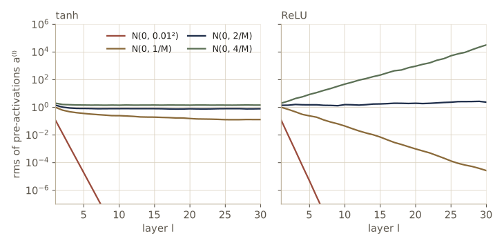
To see what is at stake, we push 200 random inputs through a 30-layer stack of width 128 and then send a random error signal back down, using the backward recursion above. We record the root mean square of the pre-activations \(a^{(l)}\) and of the backward signals at each layer, for four weight scales.
def deep_stack(h, dh, eps, L=30, M=128, N=200, rng=rng):
    """Forward N random inputs through L layers of width M (weights N(0, eps^2)), then
    pass a random error signal back down. Returns the rms of a^(l) and of the backward
    signal at each layer."""
    z = rng.normal(size=(N, M))
    Ws, As, rms_a = [], [], []
    for l in range(L):
        W = rng.normal(0, eps, size=(M, M))
        a = z @ W.T                                   # a_i = sum_j w_ij z_j
        z = h(a)
        Ws.append(W); As.append(a); rms_a.append(np.sqrt(np.mean(a**2)))
    delta = rng.normal(size=(N, M))                   # error signal arriving at the top
    rms_d = []
    for W, a in zip(Ws[::-1], As[::-1]):
        delta = (delta * dh(a)) @ W                   # chain rule one layer down
        rms_d.append(np.sqrt(np.mean(delta**2)))
    return np.array(rms_a), np.array(rms_d[::-1])

relu, d_relu = (lambda a: np.maximum(a, 0)), (lambda a: (a > 0).astype(float))
d_tanh = lambda a: 1 - np.tanh(a) ** 2
scales = {"N(0, 0.01^2)": lambda M: 0.01, "N(0, 1/M)": lambda M: np.sqrt(1 / M),
          "N(0, 2/M)": lambda M: np.sqrt(2 / M), "N(0, 4/M)": lambda M: np.sqrt(4 / M)}

stack_results = {}
print("                         rms of a: layer 1        10        30    backward: layer 1")
for act, (h, dh) in {"tanh": (np.tanh, d_tanh), "ReLU": (relu, d_relu)}.items():
    for name, eps_fn in scales.items():
        rms_a, rms_d = deep_stack(h, dh, eps_fn(128))
        stack_results[act, name] = (rms_a, rms_d)
        print(f"{act:4s}  {name:13s}   {rms_a[0]:9.3g} {rms_a[9]:9.3g} {rms_a[29]:9.3g}"
              f"      {rms_d[0]:9.3g}")
                         rms of a: layer 1        10        30    backward: layer 1
tanh  N(0, 0.01^2)        0.114  3.42e-10   3.9e-29       4.34e-29
tanh  N(0, 1/M)           0.993      0.25      0.13          0.146
tanh  N(0, 2/M)            1.43     0.808      0.79           2.98
tanh  N(0, 4/M)            1.98      1.43      1.45           92.3
ReLU  N(0, 0.01^2)        0.115  1.56e-11  1.32e-33       1.37e-33
ReLU  N(0, 1/M)            1.01    0.0443  2.65e-05       3.15e-05
ReLU  N(0, 2/M)             1.4      1.57      2.36           1.01
ReLU  N(0, 4/M)               2        48  3.28e+04       2.81e+04
The table tells the story of the formulas. With tiny weights, \(\mathcal{N}(0, 0.01^2)\), each layer multiplies the scale by about \(\sqrt{128} \times 0.01 \approx 0.11\) (and ReLU by a further \(1/\sqrt{2}\)), and after 30 layers the activations and the gradients reaching the first layer are around \(10^{-29}\) or smaller: nothing can be learned. For ReLU, the scale \(1/M\) still loses a factor \(\sqrt{2}\) per layer and \(4/M\) gains one, so after 30 layers the activations are off by factors of about \(10^{-5}\) and \(10^{4}\); only He’s \(2/M\) keeps them of order one. The first layer is the exception in each row, because its input is Gaussian rather than the output of a previous ReLU.
For tanh the picture is subtler. The rule \(1/M\) lets both signals decay only slowly, to about 0.13 forward and 0.15 backward after 30 layers. The forward decay happens because \(\tanh\) is flatter than the identity away from zero and so shrinks what it passes on. Larger weights keep the forward pass alive but let the backward signal grow toward the bottom of the stack, by a factor of about 90 at \(4/M\). No single scale is perfect for a deep tanh stack, which is one reason ReLU networks with He initialization became the default, and one motivation for the normalization layers at the end of this module.
PyTorch implements these rules in torch.nn.init. For a weight matrix of shape (M', M), “fan in” is \(M\) and “fan out” is \(M'\). We check that the samples have the standard deviations the formulas predict.
Wt = torch.empty(300, 500, dtype=torch.float64)       # M' = 300 outputs, M = 500 inputs
torch.nn.init.kaiming_normal_(Wt, nonlinearity="relu")
print(f"He:     sample std {Wt.std().item():.5f}   sqrt(2/M) = {np.sqrt(2 / 500):.5f}")
torch.nn.init.xavier_normal_(Wt)
print(f"Xavier: sample std {Wt.std().item():.5f}   sqrt(2/(M + M')) = {np.sqrt(2 / 800):.5f}")
He:     sample std 0.06313   sqrt(2/M) = 0.06325
Xavier: sample std 0.05005   sqrt(2/(M + M')) = 0.05000
Two further practical points. Biases are commonly initialized to zero, or, for ReLU units, to a small positive value so that most units start in their active region and receive a gradient. And the most effective initialization of all is often not random: starting from the weights of a network already trained on a related task, transfer learning as described in module 06, usually beats any random start when such a network exists. Finally, the scale \(\epsilon\) can simply be treated as a hyperparameter and tuned on validation data.
Convergence
We saw that on a quadratic error, gradient descent shrinks the distance along each eigenvector of the Hessian by the factor \(1 - \eta\lambda_i\) per step. The picture to keep in mind is a long, narrow valley. Across the valley the curvature \(\lambda_{\max}\) is high, so \(\eta\) must stay below \(2/\lambda_{\max}\) or the iterates bounce from wall to wall with growing amplitude. Along the valley floor the curvature \(\lambda_{\min}\) is low, and with that small \(\eta\) the progress there is slow. At most points the negative gradient points mostly across the valley, not along it, so the iterates zigzag. The methods in this section are different answers to that problem.
Momentum
The idea of momentum is to give the iterate some inertia, so that it keeps moving in directions where the gradient is consistent and averages out the directions where it keeps flipping. The update adds a fraction \(\mu\) of the previous step to the gradient step:
\[\Delta\mathbf{w}^{(\tau)} = -\eta \nabla E\big(\mathbf{w}^{(\tau)}\big) + \mu\, \Delta\mathbf{w}^{(\tau - 1)}, \qquad \mathbf{w}^{(\tau + 1)} = \mathbf{w}^{(\tau)} + \Delta\mathbf{w}^{(\tau)},\]with \(\Delta\mathbf{w}^{(-1)} = \mathbf{0}\) and a momentum parameter \(0 \le \mu < 1\), typically 0.9. This is also called the heavy-ball method, after the picture of a ball rolling on the error surface.
Two limiting cases show what momentum does. On a gently sloping part of the surface, where the gradient \(\mathbf{g}\) hardly changes from step to step, unrolling the recursion gives a geometric series,
\[\Delta\mathbf{w} = -\eta\, \mathbf{g}\, (1 + \mu + \mu^2 + \cdots) = -\frac{\eta}{1 - \mu}\, \mathbf{g} ,\]so the effective learning rate grows from \(\eta\) to \(\eta/(1 - \mu)\), tenfold for \(\mu = 0.9\). Across a narrow valley, where the gradient alternates in sign from step to step, the same series alternates, \(-\eta\, \mathbf{g}\,(1 - \mu + \mu^2 - \cdots) = -\eta\, \mathbf{g}/(1 + \mu)\), and the effective rate drops to about \(\eta/2\). Momentum speeds up exactly the directions gradient descent handles badly and calms the ones that oscillate.
On a quadratic we can say precisely how much it helps. Along eigenvector \(\mathbf{u}_i\) the update becomes \(\alpha_i^{(\tau+1)} = \alpha_i^{(\tau)} - \eta\lambda_i\alpha_i^{(\tau)} + \mu\big(\alpha_i^{(\tau)} - \alpha_i^{(\tau-1)}\big)\), a two-term linear recurrence:
\[\begin{pmatrix} \alpha_i^{(\tau+1)} \\ \alpha_i^{(\tau)} \end{pmatrix} = \begin{pmatrix} 1 + \mu - \eta\lambda_i & -\mu \\ 1 & 0 \end{pmatrix} \begin{pmatrix} \alpha_i^{(\tau)} \\ \alpha_i^{(\tau-1)} \end{pmatrix}.\]The convergence factor per step is the largest magnitude of an eigenvalue \(z\) of this \(2 \times 2\) matrix, the roots of \(z^2 - (1 + \mu - \eta\lambda_i)\,z + \mu = 0\). The product of the two roots is \(\mu\). When they are complex (a damped oscillation), they are conjugates of equal magnitude, so both have magnitude exactly \(\sqrt{\mu}\), whatever the value of \(\lambda_i\). The roots are complex when the discriminant is negative, \((1 + \mu - \eta\lambda_i)^2 < 4\mu\), which rearranges to
\[(1 - \sqrt{\mu})^2 < \eta\lambda_i < (1 + \sqrt{\mu})^2 .\]If we choose \(\eta\) and \(\mu\) so that every eigenvalue from \(\lambda_{\min}\) to \(\lambda_{\max}\) lands in this window, every direction converges at the same rate \(\sqrt{\mu}\). The window can hold a ratio \(\lambda_{\max}/\lambda_{\min}\) of at most \(\big((1 + \sqrt{\mu})/(1 - \sqrt{\mu})\big)^2\), so the smallest \(\mu\) that covers condition number \(\kappa\) satisfies \((1 + \sqrt{\mu})/(1 - \sqrt{\mu}) = \sqrt{\kappa}\).
Result. With \(\sqrt{\mu} = (\sqrt{\kappa} - 1)/(\sqrt{\kappa} + 1)\) and \(\eta = 4/(\sqrt{\lambda_{\max}} + \sqrt{\lambda_{\min}})^2\), the heavy-ball method converges on a quadratic at the rate
\[\rho = \frac{\sqrt{\kappa} - 1}{\sqrt{\kappa} + 1} \approx 1 - \frac{2}{\sqrt{\kappa}},\]compared with \((\kappa - 1)/(\kappa + 1) \approx 1 - 2/\kappa\) for the best plain gradient descent. The number of steps grows like \(\sqrt{\kappa}\) instead of \(\kappa\).
For \(\kappa = 1000\) that is the difference between thousands of steps and a few hundred. In practice we do not know \(\kappa\), and \(\mu = 0.9\) is a robust default, but the analysis explains why momentum helps most on badly conditioned problems.
Nesterov momentum
A variant called Nesterov momentum (Nesterov’s accelerated gradient) changes the order of operations. Heavy-ball momentum evaluates the gradient where we are and then adds the momentum step. Nesterov first takes the momentum step, looks at the gradient at the point it leads to, and corrects from there:
\[\Delta\mathbf{w}^{(\tau)} = -\eta \nabla E\big(\mathbf{w}^{(\tau)} + \mu\,\Delta\mathbf{w}^{(\tau-1)}\big) + \mu\, \Delta\mathbf{w}^{(\tau - 1)}.\]Evaluating the gradient at the look-ahead point lets the method react to a change in slope one step earlier, which damps the overshoot of heavy-ball momentum. For batch gradient descent on convex problems it provably improves the worst-case rate; with noisy mini-batch gradients the advantage is smaller.
Implementations usually store the look-ahead point instead of \(\mathbf{w}\), so that the gradient is always taken at the stored parameters. Let \(\widehat{\mathbf{w}}^{(\tau)} = \mathbf{w}^{(\tau)} + \mu\,\Delta\mathbf{w}^{(\tau - 1)}\) and \(\mathbf{g} = \nabla E(\widehat{\mathbf{w}}^{(\tau)})\), so the update above reads \(\Delta\mathbf{w}^{(\tau)} = \mu\,\Delta\mathbf{w}^{(\tau-1)} - \eta\,\mathbf{g}\). Then
\[\begin{aligned} \widehat{\mathbf{w}}^{(\tau+1)} &= \mathbf{w}^{(\tau)} + \Delta\mathbf{w}^{(\tau)} + \mu\,\Delta\mathbf{w}^{(\tau)} \\ &= \widehat{\mathbf{w}}^{(\tau)} - \mu\,\Delta\mathbf{w}^{(\tau-1)} + \Delta\mathbf{w}^{(\tau)} + \mu\,\Delta\mathbf{w}^{(\tau)} \\ &= \widehat{\mathbf{w}}^{(\tau)} + \mu\,\Delta\mathbf{w}^{(\tau)} - \eta\,\mathbf{g}, \end{aligned}\]using \(\Delta\mathbf{w}^{(\tau)} - \mu\,\Delta\mathbf{w}^{(\tau-1)} = -\eta\,\mathbf{g}\) in the last line. So in the shifted variables Nesterov momentum is: compute the gradient at the current parameters, update the step \(\Delta\mathbf{w} \leftarrow \mu\,\Delta\mathbf{w} - \eta\,\mathbf{g}\), and move by \(\mu\,\Delta\mathbf{w} - \eta\,\mathbf{g}\) (heavy-ball would move by \(\Delta\mathbf{w}\)). That is one extra line of code.
Our optimizers all follow one pattern: the constructor receives a list of parameter arrays, and step(grads) updates those arrays in place, so the same object can drive a NumPy vector or the weights of a PyTorch model.
class SGD:
    """Gradient descent with optional heavy-ball or Nesterov momentum.
    dw <- mu dw - lr g;  w <- w + dw  (heavy ball)  or  w <- w + mu dw - lr g  (Nesterov)."""
    def __init__(self, params, lr, momentum=0.0, nesterov=False):
        self.params, self.lr, self.mu, self.nesterov = params, lr, momentum, nesterov
        self.dw = [np.zeros_like(p) for p in params]          # the previous step Delta w

    def step(self, grads):
        for p, g, dw in zip(self.params, grads, self.dw):
            dw *= self.mu
            dw -= self.lr * g                                 # Delta w = mu Delta w - eta g
            if self.nesterov:
                p += self.mu * dw - self.lr * g
            else:
                p += dw

def run_on_quadratic(make_opt, H, w_star, tol=1e-6, max_steps=100_000):
    """Steps until ||w - w*|| < tol ||w*|| (from w = 0), and the final per-step rate."""
    w = np.zeros_like(w_star)
    opt = make_opt([w])
    dist = [np.linalg.norm(w_star)]
    for tau in range(1, max_steps + 1):
        opt.step([H @ (w - w_star)])
        dist.append(np.linalg.norm(w - w_star))
        if dist[-1] < tol * dist[0]:
            break
    k = min(50, tau // 2)
    return tau, (dist[-1] / dist[-1 - k]) ** (1 / k)

lam_min, lam_max = 1.0, 1000.0                   # the kappa = 1000 problem from above
kappa = lam_max / lam_min
mu_opt = ((np.sqrt(kappa) - 1) / (np.sqrt(kappa) + 1)) ** 2
eta_opt = 4 / (np.sqrt(lam_max) + np.sqrt(lam_min)) ** 2
runs = {"GD, eta = 2/(lam_min+lam_max)":        lambda p: SGD(p, 2 / (lam_min + lam_max)),
        "momentum 0.9, eta = 1/lam_max":         lambda p: SGD(p, 1 / lam_max, 0.9),
        "Nesterov 0.9, eta = 1/lam_max":         lambda p: SGD(p, 1 / lam_max, 0.9, True),
        f"momentum {mu_opt:.4f}, eta = {eta_opt:.2e}": lambda p: SGD(p, eta_opt, mu_opt)}
for name, make_opt in runs.items():
    steps, rate = run_on_quadratic(make_opt, H_1000, w_1000)
    print(f"{name:37s} {steps:6d} steps, measured rate {rate:.4f}")
print(f"predicted: GD {(kappa - 1) / (kappa + 1):.4f}, tuned momentum {np.sqrt(mu_opt):.4f}")
GD, eta = 2/(lam_min+lam_max)           6363 steps, measured rate 0.9980
momentum 0.9, eta = 1/lam_max           1127 steps, measured rate 0.9889
Nesterov 0.9, eta = 1/lam_max           1138 steps, measured rate 0.9890
momentum 0.8811, eta = 3.76e-03          295 steps, measured rate 0.9422
predicted: GD 0.9980, tuned momentum 0.9387
On the problem with \(\kappa = 1000\), the best plain gradient descent needs 6363 steps, at exactly its predicted rate. Momentum with the default \(\mu = 0.9\) needs between five and six times fewer, and Nesterov behaves almost the same here. With the tuned values from the result above, momentum finishes in 295 steps, more than twenty times fewer than gradient descent. Its measured rate, 0.9422, is a little above the predicted \(\sqrt{\mu} = 0.9387\). The reason is that at the two ends of the spectrum the tuned settings make the two roots coincide, and a repeated root adds a factor that grows like \(\tau\) in front of \(\rho^{\tau}\), which slows the observed rate slightly over a finite run.
Now the check against PyTorch. PyTorch writes momentum with a “buffer” \(\mathbf{v} \leftarrow \mu\mathbf{v} + \mathbf{g}\) and the step \(\mathbf{w} \leftarrow \mathbf{w} - \eta\,\mathbf{v}\) (heavy ball) or \(\mathbf{w} \leftarrow \mathbf{w} - \eta(\mathbf{g} + \mu\mathbf{v})\) (Nesterov). With a constant \(\eta\) this is our update with \(\Delta\mathbf{w} = -\eta\,\mathbf{v}\). To compare, we minimize a small logistic regression error with both implementations, feeding each the same NumPy gradient at its own current parameters, and report the largest difference in the parameters after 25 steps.
N_lr, D_lr = 200, 5
X_lr = rng.normal(size=(N_lr, D_lr))
t_lr = (X_lr @ rng.normal(size=D_lr) + 0.5 * rng.normal(size=N_lr) > 0).astype(float)

def logistic_grads(w, b):
    """Gradients of the mean cross-entropy of a logistic regression model."""
    y = 1 / (1 + np.exp(-(X_lr @ w + b)))
    return [X_lr.T @ (y - t_lr) / N_lr, np.array((y - t_lr).mean())]

def compare_with_torch(make_ours, make_torch, steps=25, seed=0):
    """Run our optimizer and a torch.optim one side by side; max parameter difference."""
    r = np.random.default_rng(seed)
    start = [r.normal(size=D_lr), np.array(0.3)]
    ours = [p.copy() for p in start]
    theirs = [torch.tensor(p.copy(), requires_grad=True) for p in start]
    opt_ours, opt_torch = make_ours(ours), make_torch(theirs)
    for _ in range(steps):
        opt_ours.step(logistic_grads(*ours))
        for p, g in zip(theirs, logistic_grads(*[q.detach().numpy() for q in theirs])):
            p.grad = torch.from_numpy(g)
        opt_torch.step()
    return max(np.abs(a - b.detach().numpy()).max() for a, b in zip(ours, theirs))

checks = {"SGD":      (lambda p: SGD(p, 0.5),
                       lambda p: torch.optim.SGD(p, lr=0.5)),
          "momentum": (lambda p: SGD(p, 0.5, 0.9),
                       lambda p: torch.optim.SGD(p, lr=0.5, momentum=0.9)),
          "Nesterov": (lambda p: SGD(p, 0.5, 0.9, True),
                       lambda p: torch.optim.SGD(p, lr=0.5, momentum=0.9, nesterov=True))}
for name, (ours, theirs) in checks.items():
    print(f"{name:9s} max difference after 25 steps: {compare_with_torch(ours, theirs):.1e}")
SGD       max difference after 25 steps: 0.0e+00
momentum  max difference after 25 steps: 0.0e+00
Nesterov  max difference after 25 steps: 0.0e+00
The trajectories agree to rounding error.
Watch out. The two ways of writing momentum agree only while \(\eta\) is constant. If the learning rate changes, PyTorch’s buffer \(\mathbf{v}\) carries past gradients that get multiplied by the new \(\eta\), while \(\Delta\mathbf{w}\) carries past steps made with the old one. Both are reasonable, but a schedule tuned for one convention can behave differently in the other.
Learning-rate schedules
So far \(\eta\) has been fixed. With stochastic gradients that is a problem, as the SGD run above showed: near the minimum the true gradient becomes small, but the mini-batch gradient does not, because its noise does not vanish there. With a fixed step size the iterates keep hopping around the minimum at a distance that grows with \(\eta\). A large \(\eta\) gives fast early progress and a high floor; a small \(\eta\) gives a low floor and slow progress. The usual resolution is a learning-rate schedule: start large and decrease \(\eta\) as training proceeds, writing \(\eta^{(\tau)}\) for the rate at step \(\tau\).
Common schedules, with \(\eta_0\) the initial rate and \(T\) the total number of steps:
| Schedule | \(\eta^{(\tau)}\) | Typical use |
|---|---|---|
| Linear decay | \((1 - \tau/K)\,\eta_0 + (\tau/K)\,\eta_K\) for \(\tau \le K\), then \(\eta_K\) | simple decay to a floor |
| Power law | \(\eta_0\,(1 + \tau/s)^{c}\), \(c < 0\) | classical stochastic approximation (\(c = -1\)) |
| Exponential | \(\eta_0\, c^{\tau/s}\), \(0 < c < 1\) | smooth decay by a factor \(c\) every \(s\) steps |
| Step | \(\eta_0\, c^{\lfloor \tau/s \rfloor}\) | drop by a factor (often 10) at fixed epochs |
| Cosine | \(\eta_{\min} + \tfrac12(\eta_0 - \eta_{\min})\{1 + \cos(\pi\tau/T)\}\) | smooth decay to \(\eta_{\min}\) at the end of training |
| Linear warmup | \(\eta_0 \min(1, (\tau + 1)/T_w)\), then any of the above | first few hundred or thousand steps, especially with Adam and transformers |
Warmup runs the other way: it starts with a small rate and ramps it up over the first \(T_w\) steps. At the start of training the weights are random and the gradients can be large and erratic, and adaptive methods (below) have not yet collected reliable statistics, so a gentle start avoids early steps that throw the network into a bad region. Transformers (module 12) are commonly trained with warmup followed by a decay. The hyperparameters (\(\eta_0\), the decay constants, \(T_w\)) are chosen empirically, and the most useful diagnostic is the learning curve, the training error plotted against the step count, watched as training runs.
def lr_linear(tau, eta0, etaK, K):
    return eta0 + (etaK - eta0) * min(tau, K) / K

def lr_power(tau, eta0, s, c):
    return eta0 * (1 + tau / s) ** c

def lr_exponential(tau, eta0, s, c):
    return eta0 * c ** (tau / s)

def lr_step(tau, eta0, s, c):
    return eta0 * c ** (tau // s)

def lr_cosine(tau, eta0, T, eta_min=0.0):
    return eta_min + 0.5 * (eta0 - eta_min) * (1 + np.cos(np.pi * min(tau, T) / T))

def with_warmup(schedule, T_w):
    """Multiply any schedule by a linear ramp over the first T_w steps."""
    return lambda tau, *args: min(1.0, (tau + 1) / T_w) * schedule(tau, *args)

# check against torch.optim.lr_scheduler over 100 steps
def torch_rates(make_sched, T=100, eta0=0.1):
    opt = torch.optim.SGD([torch.zeros(1, requires_grad=True)], lr=eta0)
    sched, rates = make_sched(opt), []
    for _ in range(T):
        rates.append(opt.param_groups[0]["lr"])
        opt.step(); sched.step()
    return np.array(rates)

S = torch.optim.lr_scheduler
taus = range(100)
pairs = {"step":        (S.StepLR, dict(step_size=30, gamma=0.1),
                         lambda t: lr_step(t, 0.1, 30, 0.1)),
         "exponential": (S.ExponentialLR, dict(gamma=0.97),
                         lambda t: lr_exponential(t, 0.1, 1, 0.97)),
         "cosine":      (S.CosineAnnealingLR, dict(T_max=100),
                         lambda t: lr_cosine(t, 0.1, 100)),
         "linear":      (S.LinearLR, dict(start_factor=1.0, end_factor=0.1, total_iters=80),
                         lambda t: lr_linear(t, 0.1, 0.01, 80))}
for name, (cls, kw, ours) in pairs.items():
    same = np.allclose(torch_rates(lambda o: cls(o, **kw)), [ours(t) for t in taus])
    print(f"{name:12s} matches torch: {same}")
step         matches torch: True
exponential  matches torch: True
cosine       matches torch: True
linear       matches torch: True
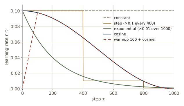
To see why decay matters, we go back to the regression problem and run mini-batch SGD with \(B = 10\) for 20 epochs (4000 steps) under four schedules, measuring how far above the minimum each run ends.
def run_sgd_schedule(schedule, epochs=20, B=10, seed=4):
    rng_run = np.random.default_rng(seed)
    w = np.zeros(D + 1)
    opt = SGD([w], lr=schedule(0))
    tau, trace = 0, []
    for epoch in range(epochs):
        for idx in minibatches(N, B, rng_run):
            opt.lr = schedule(tau)                    # set eta^(tau) before each step
            opt.step([grad_reg(w, idx)])
            tau += 1
        trace.append(E_reg(w) - E_min)
    return np.array(trace)

T_total = 20 * N // 10
schedules = {"constant 0.05":         lambda t: 0.05,
             "constant 0.005":        lambda t: 0.005,
             "step 0.05, x0.1 at 50%": lambda t: lr_step(t, 0.05, T_total // 2, 0.1),
             "cosine 0.05 -> 0":       lambda t: lr_cosine(t, 0.05, T_total)}
print("schedule                  E - E_min after epoch 1        5         20")
for name, sch in schedules.items():
    tr = run_sgd_schedule(sch)
    print(f"{name:24s} {tr[0]:22.2e} {tr[4]:9.2e} {tr[19]:9.2e}")
schedule                  E - E_min after epoch 1        5         20
constant 0.05                          4.11e-02  2.20e-03  1.81e-03
constant 0.005                         3.56e-01  9.65e-02  1.41e-02
step 0.05, x0.1 at 50%                 4.11e-02  2.20e-03  1.28e-04
cosine 0.05 -> 0                       4.12e-02  2.21e-03  1.86e-04
The two constant rates show the trade-off. With \(\eta = 0.05\) the error drops to about \(2 \times 10^{-3}\) within five epochs and then stalls there: that is its noise floor. With \(\eta = 0.005\) the floor would be lower, but on this ill-conditioned problem the small rate is still far from it after 20 epochs. The decaying schedules get the best of both: they move as fast as the large constant rate while \(\eta\) is large, and once it has decayed they settle about ten times closer to the minimum than the constant rate does.
AdaGrad, RMSProp, and Adam
The learning rate is limited by the most strongly curved direction, and the ideal step along each eigendirection would be about \(1/\lambda_i\). We usually cannot afford the Hessian, but a cheap idea goes a long way: give each parameter its own learning rate, adapted from the history of its own gradients. A parameter whose gradients are consistently large gets smaller steps, and one whose gradients are small gets larger steps. This matches the curvature argument only if the Hessian’s eigenvectors are roughly aligned with the coordinate axes, which in a network they generally are not. Still, these adaptive methods work well in practice and are the default choice for many architectures.
AdaGrad (adaptive gradient) divides each parameter’s step by the root of the accumulated sum of its squared gradients. Writing \(g_i = \partial E/\partial w_i\) for the mini-batch gradient at step \(\tau\),
\[r_i^{(\tau)} = r_i^{(\tau-1)} + g_i^2, \qquad w_i^{(\tau)} = w_i^{(\tau-1)} - \frac{\eta}{\sqrt{r_i^{(\tau)}} + \delta}\, g_i,\]starting from \(r_i^{(0)} = 0\), with a small \(\delta\) (such as \(10^{-8}\) or \(10^{-10}\)) to avoid division by zero. Parameters that have seen large gradients slow down quickly. The weakness is that \(r_i\) only grows, so the effective rates shrink throughout training and can become too small to make progress late on.
RMSProp (root mean square propagation) replaces the sum with an exponentially weighted moving average, so that old gradients are forgotten:
\[r_i^{(\tau)} = \beta\, r_i^{(\tau-1)} + (1 - \beta)\, g_i^2, \qquad w_i^{(\tau)} = w_i^{(\tau-1)} - \frac{\eta}{\sqrt{r_i^{(\tau)}} + \delta}\, g_i,\]with \(0 < \beta < 1\), typically 0.9 or 0.99 (PyTorch’s default is 0.99). Now \(\sqrt{r_i}\) tracks the recent root mean square gradient, and the step size stays roughly \(\eta\) in units of the typical gradient.
Adam (adaptive moments) combines RMSProp with momentum. It keeps moving averages of both the gradient and its square,
\[s_i^{(\tau)} = \beta_1 s_i^{(\tau-1)} + (1 - \beta_1)\, g_i, \qquad r_i^{(\tau)} = \beta_2 r_i^{(\tau-1)} + (1 - \beta_2)\, g_i^2,\]corrects both for their start at zero,
\[\widehat{s}_i^{(\tau)} = \frac{s_i^{(\tau)}}{1 - \beta_1^{\tau}}, \qquad \widehat{r}_i^{(\tau)} = \frac{r_i^{(\tau)}}{1 - \beta_2^{\tau}},\]and steps by
\[w_i^{(\tau)} = w_i^{(\tau-1)} - \eta\, \frac{\widehat{s}_i^{(\tau)}}{\sqrt{\widehat{r}_i^{(\tau)}} + \delta} .\]Common settings are \(\beta_1 = 0.9\) and \(\beta_2\) between 0.99 and 0.999 (PyTorch’s defaults are \(\beta_1 = 0.9\), \(\beta_2 = 0.999\), \(\delta = 10^{-8}\)), with \(\eta = 10^{-3}\) as a common starting point. Adam is the most widely used optimizer in deep learning.
Different sources put \(\delta\) in different places: inside the square root (\(\sqrt{r_i + \delta}\)) or outside (\(\sqrt{r_i} + \delta\)). Bishop & Bishop write it inside; PyTorch, and our code, put it outside. With \(\delta\) tiny the difference rarely matters, but it does change results slightly, so match the convention when you compare against a library.
Why the bias correction? Unroll the moving average from \(s^{(0)} = 0\):
\[s^{(\tau)} = (1 - \beta_1) \sum_{k=1}^{\tau} \beta_1^{\tau - k}\, g^{(k)} .\]If the gradients have a constant expected value \(\bar{g}\), then using the geometric sum \(\sum_{k=1}^{\tau}\beta_1^{\tau-k} = (1 - \beta_1^{\tau})/(1 - \beta_1)\),
\[\mathbb{E}\big[s^{(\tau)}\big] = (1 - \beta_1)\,\bar{g} \sum_{k=1}^{\tau} \beta_1^{\tau - k} = (1 - \beta_1^{\tau})\, \bar{g} .\]The average is biased toward zero, by the factor \(1 - \beta_1^{\tau}\), because the zero it started from still carries weight \(\beta_1^{\tau}\). Dividing by \(1 - \beta_1^{\tau}\) removes the bias exactly; the same argument applies to \(r\) with \(\beta_2\). The factors tend to one as \(\tau\) grows, so the correction only matters early, but early is when it matters most. With \(\beta_2 = 0.999\) the uncorrected \(r\) needs thousands of steps to warm up. In the very first step, the uncorrected ratio is \(s/\sqrt{r} = (1 - \beta_1)\,g / \big(\sqrt{1 - \beta_2}\,\lvert g \rvert\big) \approx 3.2 \operatorname{sign}(g)\) for the default settings, so the first steps would be more than three times larger than intended. With the correction the first step is exactly \(\eta \operatorname{sign}(g)\) (up to \(\delta\)). We can see this with a constant gradient \(g = 2\):
beta1, beta2, g = 0.9, 0.999, 2.0
s = r = 0.0
print("  tau      s     s_hat         r   r_hat   uncorrected s/sqrt(r)   corrected")
for tau in range(1, 1001):
    s = beta1 * s + (1 - beta1) * g
    r = beta2 * r + (1 - beta2) * g * g
    if tau in (1, 2, 5, 10, 100, 1000):
        s_hat, r_hat = s / (1 - beta1**tau), r / (1 - beta2**tau)
        print(f"{tau:5d} {s:6.3f} {s_hat:9.3f} {r:9.4f} {r_hat:7.3f}"
              f" {s / np.sqrt(r):23.3f} {s_hat / np.sqrt(r_hat):11.3f}")
  tau      s     s_hat         r   r_hat   uncorrected s/sqrt(r)   corrected
    1  0.200     2.000    0.0040   4.000                   3.162       1.000
    2  0.380     2.000    0.0080   4.000                   4.250       1.000
    5  0.819     2.000    0.0200   4.000                   5.797       1.000
   10  1.303     2.000    0.0398   4.000                   6.528       1.000
  100  2.000     2.000    0.3808   4.000                   3.241       1.000
 1000  2.000     2.000    2.5292   4.000                   1.258       1.000
The corrected averages equal the true values 2 and 4 from the first step, and the step ratio is 1 throughout. Without the correction the ratio starts at 3.16, climbs above 6 by step 10 (the average \(s\) warms up within a few dozen steps, \(r\) much more slowly), is still 3.24 after 100 steps, and 1.26 after 1000, when \(r\) has reached only 63% of its target value 4.
Now the three adaptive methods in code, followed by the comparison with PyTorch.
class AdaGrad:
    """r <- r + g^2;  w <- w - lr g / (sqrt(r) + delta)."""
    def __init__(self, params, lr, delta=1e-10):
        self.params, self.lr, self.delta = params, lr, delta
        self.r = [np.zeros_like(p) for p in params]

    def step(self, grads):
        for p, g, r in zip(self.params, grads, self.r):
            r += g * g
            p -= self.lr * g / (np.sqrt(r) + self.delta)

class RMSProp:
    """r <- beta r + (1 - beta) g^2;  w <- w - lr g / (sqrt(r) + delta)."""
    def __init__(self, params, lr, beta=0.99, delta=1e-8):
        self.params, self.lr, self.beta, self.delta = params, lr, beta, delta
        self.r = [np.zeros_like(p) for p in params]

    def step(self, grads):
        for p, g, r in zip(self.params, grads, self.r):
            r *= self.beta
            r += (1 - self.beta) * g * g
            p -= self.lr * g / (np.sqrt(r) + self.delta)

class Adam:
    """Moving averages s (gradient) and r (squared gradient), bias-corrected."""
    def __init__(self, params, lr=1e-3, beta1=0.9, beta2=0.999, delta=1e-8):
        self.params, self.lr, self.b1, self.b2, self.delta = params, lr, beta1, beta2, delta
        self.s = [np.zeros_like(p) for p in params]
        self.r = [np.zeros_like(p) for p in params]
        self.tau = 0

    def step(self, grads):
        self.tau += 1
        c1, c2 = 1 - self.b1 ** self.tau, 1 - self.b2 ** self.tau     # bias corrections
        for p, g, s, r in zip(self.params, grads, self.s, self.r):
            s *= self.b1
            s += (1 - self.b1) * g
            r *= self.b2
            r += (1 - self.b2) * g * g
            p -= self.lr * (s / c1) / (np.sqrt(r / c2) + self.delta)

checks = {"AdaGrad": (lambda p: AdaGrad(p, 0.5), lambda p: torch.optim.Adagrad(p, lr=0.5)),
          "RMSProp": (lambda p: RMSProp(p, 0.05), lambda p: torch.optim.RMSprop(p, 0.05)),
          "Adam":    (lambda p: Adam(p, 0.05), lambda p: torch.optim.Adam(p, lr=0.05))}
for name, (ours, theirs) in checks.items():
    print(f"{name:8s} max difference after 25 steps: {compare_with_torch(ours, theirs):.1e}")
AdaGrad  max difference after 25 steps: 0.0e+00
RMSProp  max difference after 25 steps: 2.2e-16
Adam     max difference after 25 steps: 2.2e-16
All three agree with PyTorch to rounding error.
Comparing the optimizers on a valley
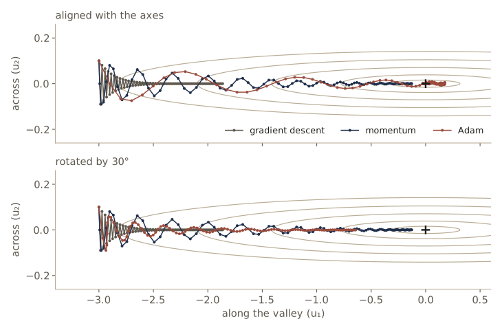
To see what the per-parameter rates buy, and when they do not help, we run the optimizers on a two-dimensional quadratic valley with curvatures 1 and 400 (\(\kappa = 400\)), twice: once with the valley aligned with the coordinate axes, and once rotated by 30°. Each optimizer gets 200 steps from the same starting point at the far end of the valley, with settings that are reasonable for each (gradient descent at \(1.9/\lambda_{\max}\), momentum 0.9 at \(1/\lambda_{\max}\)).
def rotation(theta):
    return np.array([[np.cos(theta), -np.sin(theta)], [np.sin(theta), np.cos(theta)]])

def valley(theta, lam=(1.0, 400.0)):
    """Hessian of a 2-D quadratic valley whose long axis makes angle theta with w1."""
    R = rotation(theta)
    return R @ np.diag(lam) @ R.T, R @ np.array([-3.0, 0.1])      # Hessian, starting point

valley_opts = {"gradient descent": lambda p: SGD(p, 1.9 / 400),
               "momentum":         lambda p: SGD(p, 1 / 400, 0.9),
               "Nesterov":         lambda p: SGD(p, 1 / 400, 0.9, True),
               "AdaGrad":          lambda p: AdaGrad(p, 0.5),
               "RMSProp":          lambda p: RMSProp(p, 0.05, beta=0.9),
               "Adam":             lambda p: Adam(p, 0.1)}

def run_valley(make_opt, theta, steps=200):
    H_v, w = valley(theta)
    w = w.copy()
    opt, errors = make_opt([w]), []
    for _ in range(steps):
        opt.step([H_v @ w])                        # minimum at the origin
        errors.append(0.5 * w @ H_v @ w)
    return np.array(errors)

print("E after 20, 50, 200 steps     aligned                     rotated 30°")
for name, make_opt in valley_opts.items():
    ea, er = run_valley(make_opt, 0.0), run_valley(make_opt, np.pi / 6)
    print(f"{name:17s} {ea[19]:12.1e} {ea[49]:8.1e} {ea[199]:8.1e}"
          f" {er[19]:12.1e} {er[49]:8.1e} {er[199]:8.1e}")
E after 20, 50, 200 steps     aligned                     rotated 30°
gradient descent       3.7e+00  2.8e+00  6.7e-01      3.7e+00  2.8e+00  6.7e-01
momentum               2.6e+00  3.6e-01  2.6e-06      2.6e+00  3.6e-01  2.6e-06
Nesterov               2.2e+00  3.5e-01  5.7e-06      2.2e+00  3.5e-01  5.7e-06
AdaGrad                9.3e-02  7.4e-04  2.5e-14      3.9e+00  3.1e+00  1.1e+00
RMSProp                1.7e+00  2.9e-01  1.3e-01      4.5e+00  2.8e+00  6.5e-01
Adam                   7.7e-01  1.5e-02  2.2e-09      3.4e+00  1.6e+00  2.0e-04
Three things stand out. Gradient descent, momentum, and Nesterov give identical numbers in both columns: they are rotation invariant, since rotating the problem just rotates their iterates. Momentum reduces the error by five more orders of magnitude than gradient descent in 200 steps. On the aligned valley, AdaGrad and Adam are the fastest of all, because rescaling each coordinate by its own gradient size is exactly the right fix when the curvature is axis-aligned. Rotate the valley and that advantage mostly disappears: AdaGrad becomes the slowest method, and Adam falls behind momentum. RMSProp with a constant rate never settles in either case; like Adam without its momentum average, it ends up taking steps of roughly fixed size \(\eta\) that hop back and forth across the minimum, and it needs a decaying learning rate to finish.
In practice. The adaptive methods earn their place in networks not because the Hessian is diagonal, but because different parameters (embeddings of rare and common words, weights in different layers, gain and bias parameters) see gradients of very different sizes, and a per-parameter scale evens that out without tuning. Adam with a warmup and a decaying schedule is the usual default for transformers; SGD with momentum and a step or cosine schedule remains common for convolutional networks. Both are worth trying on a new problem.
Normalization
Networks train more easily when the numbers flowing through them are of a sensible size, neither tiny nor huge, and comparable across units. In principle the weights could adapt to any scale, but in practice gradient descent struggles when they have to, for the conditioning reasons we have just seen. Normalization rescales the variables explicitly. We look at three places to do it: across the data set for the inputs, across the mini-batch for each hidden unit, and across the units of a layer for each example.
Data normalization
Suppose one input feature is measured in units that make it vary by tens (a length in centimeters, say) and another by hundredths (a concentration). For a linear model \(y = w_0 + w_1 x_1 + w_2 x_2\), a small change in \(w_1\) moves the output a thousand times more than the same change in \(w_2\), so the error surface is far more curved along \(w_1\) than along \(w_2\): exactly the narrow valley of the previous section. The fix costs nothing. Before training, compute each input’s mean and variance over the training set,
\[\mu_i = \frac{1}{N}\sum_{n=1}^{N} x_{ni}, \qquad \sigma_i^2 = \frac{1}{N}\sum_{n=1}^{N} (x_{ni} - \mu_i)^2 ,\]and replace every input by its standardized value
\[\tilde{x}_{ni} = \frac{x_{ni} - \mu_i}{\sigma_i},\]which has mean zero and unit variance over the training set. The same \(\mu_i\) and \(\sigma_i\) must be used for validation and test data (and for any data the network sees later), so that every input goes through the same transformation.
For linear regression with the mean sum-of-squares error, the Hessian is \(\mathbf{H} = \frac{1}{N}\boldsymbol{\Phi}^{\mathrm{T}}\boldsymbol{\Phi}\), where \(\boldsymbol{\Phi}\) is the design matrix with a column of ones, so we can compute its condition number directly. We compare raw inputs, inputs divided by their standard deviations but not centered, and fully standardized inputs, and count gradient descent steps (at \(\eta = 1/\lambda_{\max}\)) until the weights are within a relative distance \(10^{-6}\) of the least-squares solution.
N_dn = 500
x_len = rng.normal(50, 10, N_dn)           # a feature that varies by tens
x_conc = rng.normal(0.3, 0.05, N_dn)       # a feature that varies by hundredths
t_dn = 0.04 * x_len - 6 * x_conc + rng.normal(0, 0.2, N_dn)
X_dn = np.column_stack([x_len, x_conc])

def gd_linear_regression(X, t, tol=1e-6, max_steps=100_000):
    """Condition number of H = Phi^T Phi / N and gradient descent steps to reach w_ls."""
    Phi_dn = np.column_stack([np.ones(len(t)), X])
    H_dn, c_dn = Phi_dn.T @ Phi_dn / len(t), Phi_dn.T @ t / len(t)
    w_ls_dn = np.linalg.solve(H_dn, c_dn)
    lam = np.linalg.eigvalsh(H_dn)
    w = np.zeros(3)
    for tau in range(1, max_steps + 1):
        w -= (1 / lam[-1]) * (H_dn @ w - c_dn)          # gradient of the mean error
        if np.linalg.norm(w - w_ls_dn) < tol * np.linalg.norm(w_ls_dn):
            break
    return lam[-1] / lam[0], tau, np.linalg.norm(w - w_ls_dn) / np.linalg.norm(w_ls_dn)

mu_dn, sigma_dn = X_dn.mean(axis=0), X_dn.std(axis=0)
versions = {"raw": X_dn, "divided by sigma": X_dn / sigma_dn,
            "standardized": (X_dn - mu_dn) / sigma_dn}
print("inputs              condition number    GD steps    relative distance at the end")
for name, X_v in versions.items():
    kappa_v, steps, dist = gd_linear_regression(X_v, t_dn)
    print(f"{name:18s} {kappa_v:16.4g} {steps:11d} {dist:16.1e}")
inputs              condition number    GD steps    relative distance at the end
raw                       1.123e+06      100000          8.7e-01
divided by sigma               3545       39828          1.0e-06
standardized                  1.083           6          1.8e-07
The raw inputs give a condition number over a million, and 100,000 steps of gradient descent leave the weights far from the solution. Dividing by the standard deviations helps but still leaves a condition number in the thousands, because the inputs have large means: the bias and the weights are then strongly coupled (moving \(w_1\) shifts the output by about \(\mu_1\) on average, which \(w_0\) has to compensate). With centering as well, the condition number is close to one (the remaining 1.08 comes from the small sample correlation between the two features), and gradient descent converges in six steps. For a network the effect is not this dramatic or this exact, but standardized inputs give the first layer a well-conditioned problem, and they make the initialization rules above, which assume inputs of unit scale, apply.
Batch normalization
The same argument applies inside the network: the inputs to layer \(l\) are the outputs of layer \(l - 1\), and if they have wildly different or drifting scales, layer \(l\) faces an ill-conditioned problem. But hidden activations cannot be standardized once before training, because they change every time the weights do. Batch normalization standardizes them on the fly, using the statistics of the current mini-batch.
There is a second motivation. The gradient with respect to a weight in the first layer is a sum of products of the Jacobians of all the layers above it (Bishop & Bishop §7.4.2 writes it out; module 08 derives it). A product of many factors tends to shrink toward zero if the factors are mostly smaller than one in size and to blow up if they are mostly larger: the vanishing gradient and exploding gradient problems. We saw both in the deep-stack experiment. Careful initialization makes the product well behaved at the start of training, but the weights change as training proceeds. Batch normalization keeps renormalizing, at every layer and every step.
Consider one layer with pre-activations \(a_{ni}\) for data point \(n\) and hidden unit \(i\) (we normalize pre-activations; normalizing the activations \(z_{ni}\) instead is also used). For a mini-batch of \(K\) points, batch normalization computes, separately for each unit \(i\),
\[\mu_i = \frac{1}{K}\sum_{n=1}^{K} a_{ni}, \qquad \sigma_i^2 = \frac{1}{K}\sum_{n=1}^{K} (a_{ni} - \mu_i)^2, \qquad \widehat{a}_{ni} = \frac{a_{ni} - \mu_i}{\sqrt{\sigma_i^2 + \delta}},\]with a small \(\delta\) for numerical safety. Forcing every unit to mean zero and unit variance would restrict what the layer can represent (a tanh unit, for example, could never reach its saturated range), so the normalized value is then shifted and scaled by two learned parameters per unit:
\[\tilde{a}_{ni} = \gamma_i\, \widehat{a}_{ni} + \beta_i .\]This looks as if it undoes the normalization, since \(\gamma_i\) and \(\beta_i\) can set any mean and scale. The difference lies in how the mean and scale are parameterized. Without batch normalization, the mean and variance of \(a_{ni}\) over the batch depend on all the weights of this layer and of every layer below, in a complicated way. With it, they are controlled directly by two parameters of their own, which gradient descent finds much easier to adjust. The whole transformation is differentiable in \(\gamma_i\), \(\beta_i\), and its inputs, so it is simply another layer, usually placed after each linear layer. Two consequences: the bias of the linear layer before it becomes redundant (subtracting \(\mu_i\) removes any constant), so it is usually dropped in favor of \(\beta_i\); and the output no longer depends on the scale of the weights feeding the layer, as we check below.
At inference time there may be only one input, and a network’s prediction for an input should not depend on which other inputs happen to be in its batch. So batch normalization keeps running averages of the batch statistics during training, which play no part in the training computation, and uses them in place of \(\mu_i\) and \(\sigma_i^2\) at inference:
\[\bar{\mu}_i \leftarrow \alpha\,\bar{\mu}_i + (1 - \alpha)\,\mu_i, \qquad \bar{\sigma}_i^2 \leftarrow \alpha\,\bar{\sigma}_i^2 + (1 - \alpha)\,\sigma_i^2 ,\]with \(0 \le \alpha \le 1\) (for example 0.9). PyTorch calls \(1 - \alpha\) the “momentum” of the layer (default 0.1), and its running variance uses the unbiased batch variance \(\frac{K}{K-1}\sigma_i^2\); the normalization itself uses the biased one. Our implementation follows PyTorch so that we can compare. Bishop & Bishop average the standard deviation rather than the variance; either works.
class BatchNorm:
    """Batch normalization of pre-activations A, shape (K, M): per unit, over the batch."""
    def __init__(self, M, alpha=0.9, delta=1e-5):
        self.gamma, self.beta = np.ones(M), np.zeros(M)          # learned scale and shift
        self.run_mu, self.run_var = np.zeros(M), np.ones(M)      # running averages
        self.alpha, self.delta, self.training = alpha, delta, True

    def __call__(self, A):
        if self.training:
            K = A.shape[0]
            mu, var = A.mean(axis=0), A.var(axis=0)             # this batch's statistics
            self.run_mu = self.alpha * self.run_mu + (1 - self.alpha) * mu
            self.run_var = self.alpha * self.run_var + (1 - self.alpha) * var * K / (K - 1)
        else:
            mu, var = self.run_mu, self.run_var
        A_hat = (A - mu) / np.sqrt(var + self.delta)
        return self.gamma * A_hat + self.beta

M_bn = 6
bn = BatchNorm(M_bn)
bn_torch = torch.nn.BatchNorm1d(M_bn, momentum=0.1, eps=1e-5).double()
gamma0, beta0 = rng.uniform(0.5, 2, M_bn), rng.normal(size=M_bn)   # non-trivial gamma, beta
bn.gamma, bn.beta = gamma0.copy(), beta0.copy()
with torch.no_grad():
    bn_torch.weight.copy_(torch.from_numpy(gamma0))
    bn_torch.bias.copy_(torch.from_numpy(beta0))

train_ok = True
for step in range(5):                                          # five training mini-batches
    A = rng.normal(3.0, 2.0, size=(16, M_bn))
    train_ok &= np.allclose(bn(A), bn_torch(torch.from_numpy(A)).detach().numpy())
print("training outputs match:", train_ok)
print("running mean matches:", np.allclose(bn.run_mu, bn_torch.running_mean.numpy()),
      "  running variance matches:", np.allclose(bn.run_var, bn_torch.running_var.numpy()))
print("running mean after 5 batches:", bn.run_mu)

bn.training = False
bn_torch.eval()
A_test = rng.normal(3.0, 2.0, size=(4, M_bn))
torch_out = bn_torch(torch.from_numpy(A_test)).detach().numpy()
print("inference outputs match:", np.allclose(bn(A_test), torch_out))
training outputs match: True
running mean matches: True   running variance matches: True
running mean after 5 batches: [1.3224 1.2502 1.1579 1.1124 1.2517 1.3394]
inference outputs match: True
Everything matches. Note the running mean: after five batches it has only climbed about 40% of the way from 0 toward the true mean of 3, since \(1 - 0.9^5 \approx 0.41\). Running averages need many training steps to settle, and a network evaluated in inference mode too early, or after training on very few batches, sees wrong statistics.
Two properties are worth checking directly. The training-mode output does not change if we scale the incoming weights, since the normalization divides the scale back out. And in training mode an example’s output depends on the other examples in its batch; in inference mode it does not.
Z_in = rng.normal(size=(32, 20))            # inputs to a layer, batch of 32
W_bn = rng.normal(size=(M_bn, 20))
bn2 = BatchNorm(M_bn)
out_w = bn2(Z_in @ W_bn.T)
out_10w = bn2(Z_in @ (10 * W_bn).T)
print("scaling W by 10 changes the output by", f"{np.abs(out_w - out_10w).max():.1e}")

other = rng.normal(size=(31, 20))
out_a = bn2(Z_in @ W_bn.T)[0]                                     # example 0 in its batch
out_b = bn2(np.vstack([Z_in[:1], other]) @ W_bn.T)[0]            # example 0, other batch
print("example 0, two different batches (training mode):", out_a[:3], out_b[:3])
bn2.training = False
diff = bn2(Z_in @ W_bn.T)[0] - bn2(np.vstack([Z_in[:1], other]) @ W_bn.T)[0]
print("same comparison in inference mode, max difference:", f"{np.abs(diff).max():.1e}")
scaling W by 10 changes the output by 1.5e-06
example 0, two different batches (training mode): [-1.0667  0.1573 -0.7136] [-0.825   0.0028 -0.7213]
same comparison in inference mode, max difference: 0.0e+00
The weight-scale invariance is why batch normalization tolerates poorly scaled initializations and larger learning rates: the forward pass cannot blow up because some weights grew. We can see this in the deep ReLU stack from before, where \(\mathcal{N}(0, 4/M)\) weights made the activations grow by a factor of \(10^4\) over 30 layers. With a batch normalization layer after each linear layer, every layer’s pre-activations keep the same scale.
def deep_stack_bn(eps, L=30, M=128, N=200, rng=rng):
    """Forward pass through L layers of Linear -> BatchNorm -> ReLU; rms of each a^(l)."""
    z = rng.normal(size=(N, M))
    rms_a = []
    for l in range(L):
        a = z @ rng.normal(0, eps, size=(M, M)).T
        rms_a.append(np.sqrt(np.mean(a**2)))
        z = np.maximum(BatchNorm(M)(a), 0)
    return np.array(rms_a)

for name in ["N(0, 0.01^2)", "N(0, 4/M)"]:
    without = stack_results["ReLU", name][0]
    with_bn = deep_stack_bn(scales[name](128))
    print(f"{name:13s} rms of a at layer 30: without BN {without[29]:.2e},"
          f" with BN {with_bn[29]:.3f}")
N(0, 0.01^2)  rms of a at layer 30: without BN 1.32e-33, with BN 0.082
N(0, 4/M)     rms of a at layer 30: without BN 3.28e+04, with BN 1.361
With batch normalization the scale of the pre-activations is set by the weight scale of a single layer, not by a product over thirty. The backward signal is kept in check as well, but seeing that requires the backward pass through the normalization, which is an exercise once module 08 is done.
Watch out. Batch normalization behaves differently in training and inference. Forgetting to switch a model to inference mode (in PyTorch,
model.eval()) makes its predictions depend on the batch they arrive in; forgetting to switch back (model.train()) freezes the running statistics and trains with the wrong normalization. Very small batches also make \(\mu_i\) and \(\sigma_i^2\) noisy estimates, which hurts training.
Why does batch normalization work so well? It was introduced to reduce internal covariate shift, the change in the distribution of a layer’s inputs as the layers below it are updated. Later experiments (Santurkar and colleagues, 2018) found that removing the shift was not what mattered, and that batch normalization instead makes the error surface smoother, with gradients that change less abruptly from step to step, which allows larger learning rates. The question is not fully settled, but the practical effect is well established.
Layer normalization
Batch normalization depends on the mini-batch, which is a problem when batches are small, when a batch is split across several devices (each would compute its own statistics, or they would have to communicate), and in recurrent networks, where the statistics change at every time step. Layer normalization avoids the mini-batch altogether: it normalizes across the hidden units of a layer, separately for each data point. For data point \(n\) in a layer with \(M\) units,
\[\mu_n = \frac{1}{M}\sum_{i=1}^{M} a_{ni}, \qquad \sigma_n^2 = \frac{1}{M}\sum_{i=1}^{M} (a_{ni} - \mu_n)^2, \qquad \widehat{a}_{ni} = \frac{a_{ni} - \mu_n}{\sqrt{\sigma_n^2 + \delta}},\]followed by the same learned per-unit scale and shift \(\gamma_i\,\widehat{a}_{ni} + \beta_i\). Each example is normalized using only its own values, so the computation is identical in training and inference, there are no running averages to keep, and the batch size does not matter. Layer normalization was introduced for recurrent networks, and it is now the standard normalization in transformers (module 12), where it is applied to the feature vector of each token separately.
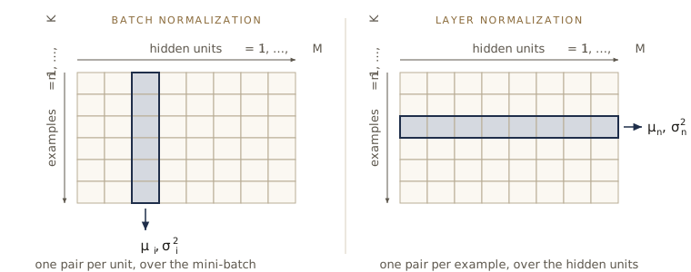
class LayerNorm:
    """Layer normalization of A with shape (K, M): per example, over the M units."""
    def __init__(self, M, delta=1e-5):
        self.gamma, self.beta, self.delta = np.ones(M), np.zeros(M), delta

    def __call__(self, A):
        mu = A.mean(axis=1, keepdims=True)
        var = A.var(axis=1, keepdims=True)
        return self.gamma * (A - mu) / np.sqrt(var + self.delta) + self.beta

ln = LayerNorm(M_bn)
ln_torch = torch.nn.LayerNorm(M_bn, eps=1e-5).double()
ln.gamma, ln.beta = gamma0.copy(), beta0.copy()
with torch.no_grad():
    ln_torch.weight.copy_(torch.from_numpy(gamma0))
    ln_torch.bias.copy_(torch.from_numpy(beta0))
A = rng.normal(3.0, 2.0, size=(4, M_bn))
torch_out = ln_torch(torch.from_numpy(A)).detach().numpy()
print("matches torch.nn.LayerNorm:", np.allclose(ln(A), torch_out))

ln2 = LayerNorm(M_bn)
H_ln = Z_in @ W_bn.T
alone = ln2(H_ln[:1])                                   # example 0 in a batch of one
in_batch = ln2(H_ln)[:1]                                # example 0 in the full batch
print(f"example 0 alone vs in a batch, max difference: {np.abs(alone - in_batch).max():.1e}")
matches torch.nn.LayerNorm: True
example 0 alone vs in a batch, max difference: 0.0e+00
The summary: batch normalization shares statistics across examples and needs reasonably large batches and a separate inference mode; layer normalization is per example and behaves the same everywhere. Batch normalization is common in convolutional networks for images (where it is computed per channel, over the batch and all spatial positions, as module 10 discusses); layer normalization is the choice for transformers and recurrent networks.
Experiment: optimizers on MNIST
We finish by training one small network with three of our optimizers. The data are the first 6000 MNIST training images and 2000 test images, flattened to 784 inputs and standardized with the training mean and standard deviation (one pair of numbers for all pixels, since they share a scale). The network has one hidden layer of 128 ReLU units, He-initialized weights and zero biases, and 10 softmax outputs trained with the cross-entropy error; that is \(784 \cdot 128 + 128 + 128 \cdot 10 + 10 = 101{,}770\) parameters. The parameters are PyTorch tensors, so autograd can compute the gradients (module 08 shows how), but the updates are made by our NumPy optimizers, which modify the tensors’ memory in place. If you want a refresher on the standard PyTorch training loop, see the EAS 510 notes on the PyTorch workflow.
train = datasets.MNIST(root="data", train=True, download=True)
test = datasets.MNIST(root="data", train=False, download=True)
X_tr = train.data[:6000].float().div(255.).reshape(-1, 784)     # (6000, 784)
y_tr = train.targets[:6000]
X_te = test.data[:2000].float().div(255.).reshape(-1, 784)      # (2000, 784)
y_te = test.targets[:2000]
pix_mu, pix_sd = X_tr.mean(), X_tr.std()                         # training statistics only
X_tr, X_te = (X_tr - pix_mu) / pix_sd, (X_te - pix_mu) / pix_sd
print(X_tr.shape, X_te.shape, f"mean {X_tr.mean().item():.3f}, std {X_tr.std().item():.3f}")
torch.Size([6000, 784]) torch.Size([2000, 784]) mean 0.000, std 1.000
def init_mlp(seed, sizes=(784, 128, 10)):
    """He-initialized weights, zero biases, as float32 torch tensors."""
    g = torch.Generator().manual_seed(seed)
    params = []
    for m_in, m_out in zip(sizes[:-1], sizes[1:]):
        W = torch.randn(m_out, m_in, generator=g) * np.sqrt(2 / m_in)     # He
        params.append(W.requires_grad_())
        params.append(torch.zeros(m_out, requires_grad=True))
    return params

def mlp(params, X):
    W1, b1, W2, b2 = params
    return torch.relu(X @ W1.T + b1) @ W2.T + b2                 # logits

def train_mlp(make_opt, epochs=6, B=64, seed=0):
    params = init_mlp(seed)
    opt = make_opt([p.data.numpy() for p in params])      # our optimizer edits the tensors
    rng_mnist = np.random.default_rng(seed)
    batch_losses, epoch_losses = [], []
    for epoch in range(epochs):
        for idx in minibatches(len(X_tr), B, rng_mnist):
            idx = torch.from_numpy(idx)
            loss = F.cross_entropy(mlp(params, X_tr[idx]), y_tr[idx])
            grads = torch.autograd.grad(loss, params)
            opt.step([g.numpy() for g in grads])
            batch_losses.append(loss.item())
        with torch.no_grad():
            epoch_losses.append(F.cross_entropy(mlp(params, X_tr), y_tr).item())
    with torch.no_grad():
        accuracy = (mlp(params, X_te).argmax(dim=1) == y_te).double().mean().item()
    return np.array(batch_losses), np.array(epoch_losses), accuracy

mnist_runs = {"SGD, eta = 0.1":                  lambda p: SGD(p, 0.1),
              "momentum 0.9, eta = 0.01":        lambda p: SGD(p, 0.01, 0.9),
              "momentum 0.9, eta = 0.05":        lambda p: SGD(p, 0.05, 0.9),
              "Adam, eta = 0.001":               lambda p: Adam(p, 1e-3)}
mnist_results = {}
for name in list(mnist_runs)[:2]:
    mnist_results[name] = train_mlp(mnist_runs[name])
print("parameters:", sum(p.numel() for p in init_mlp(0)))
parameters: 101770
for name in list(mnist_runs)[2:]:
    mnist_results[name] = train_mlp(mnist_runs[name])

print("training error after epoch    1       2       4       6    test accuracy")
for name, (_, epoch_losses, acc) in mnist_results.items():
    e = epoch_losses
    print(f"{name:25s} {e[0]:7.4f} {e[1]:7.4f} {e[3]:7.4f} {e[5]:7.4f} {acc:12.1%}")
training error after epoch    1       2       4       6    test accuracy
SGD, eta = 0.1             0.2541  0.2019  0.0937  0.0557        91.0%
momentum 0.9, eta = 0.01   0.2592  0.1790  0.0957  0.0661        91.0%
momentum 0.9, eta = 0.05   0.2086  0.0959  0.0356  0.0162        91.5%
Adam, eta = 0.001          0.2750  0.1699  0.0903  0.0515        91.1%
Several results from this module show up here. Plain SGD at \(\eta = 0.1\) and momentum at \(\eta = 0.01\) with \(\mu = 0.9\) follow closely similar paths: both have an effective learning rate of 0.1 in the low-curvature regime, as the \(\eta/(1 - \mu)\) argument predicts. Momentum at \(\eta = 0.05\) has an effective rate five times larger and drives the training error down fastest. Adam at its standard setting, with nothing tuned, tracks plain SGD closely. The test accuracies land within about half a percentage point of each other, around 91%, which suggests that on this problem the optimizer mostly changes how fast we reach a good network rather than how good it is.
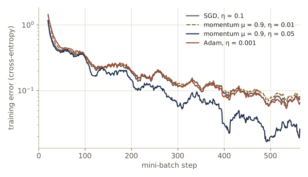
These numbers are for a small network on a tenth of MNIST, trained for six epochs on one CPU thread. On the full 60,000 images, with a GPU, more epochs, and a decaying schedule, the same network reaches roughly 97–98% test accuracy; change the slices [:6000] and [:2000] and the epochs argument to try it. The ranking of optimizers on one small problem should not be over-read: with each learning rate tuned carefully, the differences often shrink, and which one generalizes best is an empirical question for each architecture and data set.
Summary
| Method | What it does | Key formula or property |
|---|---|---|
| Local quadratic model | describes the error near a stationary point | \(E \simeq E(\mathbf{w}^{\star}) + \tfrac12\sum_i \lambda_i\alpha_i^2\); minimum iff all \(\lambda_i > 0\) |
| Batch gradient descent | steps against the full gradient | \(\alpha_i \leftarrow (1 - \eta\lambda_i)\alpha_i\); stable for \(0 < \eta < 2/\lambda_{\max}\); rate \(\approx 1 - 2/\kappa\) |
| SGD / mini-batches | noisy gradient from \(B\) points | noise variance \(\propto 1/B\); needs a decaying \(\eta\) to settle |
| He / Xavier initialization | keep signal scale constant with depth | \(\epsilon^2 = 2/M\) (ReLU), \(\epsilon^2 = 2/(M + M')\) (tanh) |
| Momentum (heavy ball) | adds inertia | effective rate \(\eta/(1 - \mu)\) on flat ground; tuned rate \(\approx 1 - 2/\sqrt{\kappa}\) |
| Nesterov momentum | gradient at the look-ahead point | in shifted variables: move by \(\mu\Delta\mathbf{w} - \eta\mathbf{g}\) |
| Learning-rate schedules | large steps early, small late | step, exponential, cosine; warmup at the start |
| AdaGrad / RMSProp | per-parameter rates from squared gradients | \(\eta/(\sqrt{r_i} + \delta)\), with \(r_i\) a sum or a moving average |
| Adam | RMSProp plus momentum, bias-corrected | \(\widehat{s}_i/(\sqrt{\widehat{r}_i} + \delta)\), corrections \(1/(1 - \beta^{\tau})\) |
| Data normalization | standardize inputs once | \(\tilde{x}_{ni} = (x_{ni} - \mu_i)/\sigma_i\) with training statistics |
| Batch normalization | standardize each unit over the mini-batch | learned \(\gamma_i, \beta_i\); running averages at inference |
| Layer normalization | standardize each example over the units | same in training and inference; used in transformers |
Ideas to carry forward:
- The Hessian’s eigenvalues govern everything local: whether a stationary point is a minimum, how large the learning rate may be, and how slowly gradient descent crawls along shallow directions. The condition number is the single most useful number for predicting optimization trouble.
- Most practical improvements attack conditioning from different sides: momentum by accumulating speed along consistent directions, adaptive methods by rescaling each parameter, and normalization by making the problem itself better conditioned.
- Depth multiplies scales. Initialization sets the per-layer gain to one at the start; normalization layers keep it near one during training.
- Stochastic gradients trade exactness for speed, and their noise sets a floor that only a decaying learning rate removes. Module 09 shows that this noise, and when we stop, also affect how well the network generalizes.
Exercises
- Show that the contours of constant error of the quadratic approximation near a minimum are ellipses (ellipsoids in higher dimensions) whose axes point along the Hessian’s eigenvectors, with semi-axis lengths proportional to \(\lambda_i^{-1/2}\). Plot the contours of the quadratic approximation at the global minimum of the toy surface on top of the true contours, and find how far from the minimum they visibly disagree.
- For linear regression with one input, \(y = w x + b\), and the mean sum-of-squares error, compute the \(2 \times 2\) Hessian with respect to \((w, b)\). Show that it is positive definite unless all the \(x_n\) are equal, and find its condition number in terms of the mean and variance of the \(x_n\). Use your formula to explain the “divided by sigma” row of the data-normalization experiment.
- Near a local minimum, show that gradient descent with \(\eta\) slightly above \(2/\lambda_{\max}\) diverges along \(\mathbf{u}_{\max}\) only. Starting very close to the minimum of the \(\kappa = 1000\) quadratic, run gradient descent with \(\eta = 2.02/\lambda_{\max}\) and verify numerically that the direction of \(\mathbf{w} - \mathbf{w}^{\star}\) lines up with \(\mathbf{u}_{\max}\).
- Let \(x_1, \dots, x_B\) be independent with mean \(\mu\) and variance \(\sigma^2\). Show that the sample mean has expected squared error \(\sigma^2/B\). Then show that if the \(B\) points are drawn without replacement from a finite population of \(N\) values with population variance \(\sigma^2\), the expected squared error is \(\frac{\sigma^2}{B}\cdot\frac{N - B}{N - 1}\), the factor used in the mini-batch experiment.
- Derive the variance recursion for a layer of ReLU units with weights drawn from the uniform distribution on \([-\epsilon, \epsilon]\) instead of a Gaussian. What value of \(\epsilon\) corresponds to He initialization? Check your answer with
deep_stack(replacerng.normalbyrng.uniform) and againsttorch.nn.init.kaiming_uniform_. - For momentum on a one-dimensional quadratic with curvature \(\lambda\), find the values of \(\eta\lambda\) for which the \(2 \times 2\) iteration matrix has real eigenvalues, and show that the method converges if and only if \(0 < \eta\lambda < 2(1 + \mu)\). Verify the boundary numerically for \(\mu = 0.9\) with
SGDon a 1-D problem. - Show that for a slowly varying gradient and small \(\eta\), the Nesterov update and the heavy-ball update produce nearly the same steps. Then find a quadratic valley and settings where Nesterov converges and heavy-ball momentum, with the same \(\eta\) and \(\mu\), does not.
- Adam is invariant to rescaling the error function. Show that multiplying \(E\) by a constant \(c > 0\) leaves Adam’s steps unchanged (apart from \(\delta\)), while it multiplies the steps of SGD by \(c\). Confirm it by running
AdamandSGDonlogistic_gradsscaled by 1000. - Implement the backward pass of
BatchNormfor the gradients with respect to \(\gamma\), \(\beta\), and the input \(\mathbf{A}\), and check it againsttorch.autogradon a small batch. (Hint: \(\mu_i\) and \(\sigma_i^2\) depend on every row of the batch, so every output row depends on every input row.) Then extenddeep_stack_bnwith a backward pass and compare the backward signal with and without batch normalization for the \(\mathcal{N}(0, 4/M)\) initialization. - Add a batch normalization layer between the linear layer and the ReLU of the MNIST network (use
torch.nn.BatchNorm1dor your own class with autograd), drop the now-redundant hidden bias, and train it with plain SGD at learning rates 0.1, 0.5, and 1.0. Compare with the network without batch normalization at the same rates. Remember to switch to inference mode before measuring the test accuracy. - Train the MNIST network with Adam using (a) a constant \(\eta = 10^{-3}\), (b) a cosine decay from \(10^{-3}\) to zero over the six epochs, and (c) a linear warmup over the first 100 steps followed by the same cosine decay. Report the training error at each epoch and the test accuracy, and plot the learning curves.
- In your own words: why does gradient descent slow down on an ill-conditioned error surface, and how do momentum, Adam, and normalization each address the problem? Explain it to a classmate who knows what a gradient is but has not seen the Hessian.
Going further
- Bishop & Bishop, Deep Learning: Foundations and Concepts, chapter 7 — the chapter this module follows. Exercises 7.1–7.3 and 7.6 (the local quadratic approximation), 7.4–7.5 (Hessians of simple models), 7.7 (counting the unknowns), 7.9 (He initialization), 7.10 (gradient descent in eigen-coordinates), 7.11 (Nesterov momentum), 7.12 (bias correction), 7.13 (line search), and 7.14 (standardization) extend the material here.
- Diederik P. Kingma and Jimmy Ba, “Adam: A method for stochastic optimization”, arXiv:1412.6980 — the Adam paper, with the bias correction argument.
- Xavier Glorot and Yoshua Bengio, “Understanding the difficulty of training deep feedforward neural networks” (AISTATS, 2010), and Kaiming He, Xiangyu Zhang, Shaoqing Ren, and Jian Sun, “Delving deep into rectifiers”, arXiv:1502.01852 — the two initialization schemes derived above.
- Sergey Ioffe and Christian Szegedy, “Batch normalization: Accelerating deep network training by reducing internal covariate shift”, arXiv:1502.03167, and Jimmy Lei Ba, Jamie Ryan Kiros, and Geoffrey E. Hinton, “Layer normalization”, arXiv:1607.06450.
- Ian Goodfellow, Yoshua Bengio, and Aaron Courville, Deep Learning (MIT Press, 2016), free online — chapter 8 covers optimization for training deep models in more depth, including second-order methods.
- Related modules: module 06 (deep networks and their symmetries), module 08 (how the gradients are computed), module 09 (how optimization interacts with generalization), module 12 (layer normalization and warmup in transformers), and Intro to ML, module 05 (the Hessian of a network and how to compute it).
These notes follow the chapters of C. M. Bishop and H. Bishop, Deep Learning: Foundations and Concepts (Springer, 2024), the course text, which the authors make free to read online. The explanations, code, figures, and exercises here are written for this course; the book remains the reference, with the full derivations and many more exercises.