CSE 676 · Module 08 · Week 4
Backpropagation
Backpropagation derived and built from scratch, gradient checking, the Jacobian and Hessian, and forward- and reverse-mode automatic differentiation.
Companion reading: Bishop & Bishop, Deep Learning: Foundations and Concepts, chapter 8, “Backpropagation”
By the end of this module you can
- Derive the backpropagation formula \(\delta_j = h'(a_j) \sum_k w_{kj} \delta_k\) for a feed-forward network of any topology, and write it in matrix form for a layered network that processes a mini-batch.
- Implement forward and backward passes for linear, tanh, ReLU, and softmax cross-entropy layers in NumPy, and check them against finite differences and PyTorch.
- Explain how truncation and round-off errors trade off in finite differences, choose a step size, and explain why numerical gradients cost \(O(W^2)\).
- Compute a network’s Jacobian by backpropagation, its Hessian exactly, by finite differences, and with the outer-product (Gauss–Newton) approximation, and form Hessian–vector products in \(O(W)\).
- Contrast symbolic, numerical, and automatic differentiation, and write a computation as an evaluation trace.
- Implement forward-mode automatic differentiation with dual numbers and reverse-mode automatic differentiation with a small scalar autograd engine, and train a network with that engine.
- Decide whether forward or reverse mode is cheaper for a function from \(\mathbb{R}^D\) to \(\mathbb{R}^K\), and explain the memory cost of reverse mode and how checkpointing reduces it.
- Train the from-scratch NumPy network on MNIST and match one of its training steps against PyTorch.
Contents
- Evaluation of gradients
- Automatic differentiation
- Training the from-scratch network on MNIST
- Summary
- Exercises
- Going further
In module 06 we built deep networks, and in module 07 we trained them with stochastic gradient descent, momentum, and Adam. Every one of those optimizers asks for the same thing at every step: the gradient \(\nabla E(\mathbf{w})\) of the error with respect to all the weights and biases, of which a modern network has millions. So far a single call, loss.backward(), has supplied it. In this module we open that box.
The method inside is error backpropagation, or backprop. A forward pass evaluates the network and keeps every intermediate value; a backward pass then sends error signals from the outputs toward the inputs, and the derivative with respect to each weight falls out as the product of two numbers that are already available at the two ends of that weight. The whole gradient costs a small constant times one forward pass. Intro to ML, module 05 derives backpropagation for a two-layer network and builds it in NumPy. Here we take the view that deep learning needs: networks of any feed-forward shape, layers written as modules with a forward and a backward method, mini-batches processed as matrices, and automatic differentiation as the general mechanism that turns code for a function into code for its derivatives.
The module has three parts. The first derives backpropagation, builds a small layered-network library in NumPy, and checks it against finite differences and PyTorch; the same machinery then gives the Jacobian and the Hessian. The second part is about automatic differentiation: we write a forward-mode differentiator based on dual numbers and a reverse-mode “autograd” engine of about fifty lines, train a network with the engine, and compare the cost of the two modes. The last part trains the NumPy library on MNIST and checks one training step against the same network in PyTorch, weight for weight.
A word on terminology. “Backpropagation” is used loosely in the literature, sometimes for a whole training procedure and sometimes even for a network architecture. We use it only for the computation of derivatives. What an optimizer then does with the gradient is a separate step, the subject of module 07.
Evaluation of gradients
Error functions built from independent data points are sums (or averages) of one term per point,
\[E(\mathbf{w}) = \sum_{n=1}^{N} E_n(\mathbf{w}).\]So it is enough to work out \(\nabla E_n\) for a single data point. Stochastic gradient descent uses it directly; a mini-batch or full-batch method adds it up over the points it uses. We will see that in matrix form the sum over a mini-batch comes for free: it turns into a matrix product.
Single-layer networks
Start with a network that has no hidden units: a linear model with outputs \(y_k = \sum_i w_{ki} x_i\) (a bias is a weight on an extra input fixed at 1) and, for data point \(n\), the sum-of-squares error
\[E_n = \frac{1}{2} \sum_{k} (y_{nk} - t_{nk})^2 .\]The weight \(w_{ki}\) affects only output \(k\), so the chain rule gives
\[\frac{\partial E_n}{\partial w_{ki}} = (y_{nk} - t_{nk})\, x_{ni} .\]This is a product of two local quantities: an error signal \(y_{nk} - t_{nk}\) at the output end of the connection and the input \(x_{ni}\) at its input end. Module 05 showed that exactly the same form holds for a logistic-sigmoid output with the binary cross-entropy and for a softmax output with the multiclass cross-entropy. In each case the output activation is the canonical link for the target distribution, and the derivative of the error with respect to the pre-activation of an output is “prediction minus target”.
For a mini-batch, stack the inputs as rows of \(\mathbf{X}\) (\(N \times D\)), the outputs as rows of \(\mathbf{Y}\) (\(N \times K\)), and the targets as rows of \(\mathbf{T}\). Summing the per-point derivatives over \(n\) is then one matrix product,
\[\nabla_{\mathbf{W}} E = (\mathbf{Y} - \mathbf{T})^{\mathrm{T}} \mathbf{X},\]a \(K \times D\) matrix, the same shape as \(\mathbf{W}\). We check this for softmax regression against PyTorch’s automatic differentiation.
import math
import time
import warnings
import numpy as np
import torch
import torch.nn.functional as F
from scipy.special import logsumexp
from torch.func import functional_call, grad, jacfwd, jacrev, jvp

np.set_printoptions(precision=4, suppress=True)
warnings.filterwarnings("ignore", category=FutureWarning)   # hide library notices
rng = np.random.default_rng(8)
torch.manual_seed(8)
def softmax(A):
    """Row-wise softmax, computed stably through log-sum-exp."""
    return np.exp(A - logsumexp(A, axis=1, keepdims=True))

N, D, K = 32, 5, 4
X = rng.normal(size=(N, D))
t = rng.integers(0, K, N)                  # class labels 0..K-1
T = np.eye(K)[t]                           # one-hot targets, shape (N, K)
W = rng.normal(size=(K, D))

Y = softmax(X @ W.T)                       # y_nk for the whole batch
grad_W = (Y - T).T @ X                     # sum_n (y_nk - t_nk) x_ni, shape (K, D)

W_t = torch.tensor(W, requires_grad=True)
E_t = F.cross_entropy(torch.tensor(X) @ W_t.T, torch.tensor(t), reduction="sum")
E_t.backward()
print("gradient shape:", grad_W.shape)
print(f"largest difference from torch.autograd: {np.abs(grad_W - W_t.grad.numpy()).max():.1e}")
gradient shape: (4, 5)
largest difference from torch.autograd: 3.6e-15
General feed-forward networks
Now take any feed-forward network. Each unit \(j\) forms a weighted sum of the values \(z_i\) of the units or inputs that send it a connection, and passes the result through an activation function:
\[a_j = \sum_{i} w_{ji} z_i, \qquad z_j = h(a_j).\]Here \(a_j\) is the pre-activation of unit \(j\) and \(z_j\) its activation; again a bias is a weight from a unit whose value is always 1. “Feed-forward” means that the connections form a directed acyclic graph, so the units can be put in a topological order, one in which every unit comes after all the units that feed it. Evaluating the units in that order is forward propagation. It is the only requirement: there may be several layers, connections that skip layers, or units with no layer structure at all.
Fix one data point, run forward propagation, and keep every \(a_j\) and \(z_j\). The error \(E_n\) depends on the weight \(w_{ji}\) only through the pre-activation \(a_j\) that the weight feeds, so
\[\frac{\partial E_n}{\partial w_{ji}} = \frac{\partial E_n}{\partial a_j} \frac{\partial a_j}{\partial w_{ji}} = \delta_j z_i, \qquad \text{where} \qquad \delta_j \equiv \frac{\partial E_n}{\partial a_j} .\]We used \(\partial a_j / \partial w_{ji} = z_i\). The quantity \(\delta_j\) is called the error of unit \(j\). The formula has the same shape as the single-layer case: the error at the output end of the weight times the activation at its input end. So all we need is \(\delta_j\) for every unit that is not an input.
For an output unit with the canonical link, \(\delta_k = y_k - t_k\), as before. For any other unit \(j\), the error depends on \(a_j\) only through the pre-activations \(a_k\) of the units \(k\) that \(j\) sends connections to, its children in the graph. The multivariable chain rule sums over those paths:
\[\delta_j = \frac{\partial E_n}{\partial a_j} = \sum_{k \in \mathrm{ch}(j)} \frac{\partial E_n}{\partial a_k} \frac{\partial a_k}{\partial a_j} .\]Since \(a_k = \sum_{j'} w_{kj'} h(a_{j'})\), we have \(\partial a_k / \partial a_j = w_{kj} h'(a_j)\), and so
\[\delta_j = h'(a_j) \sum_{k \in \mathrm{ch}(j)} w_{kj} \delta_k .\]This is the backpropagation formula. The error of a unit is the weighted sum of the errors of its children, scaled by the slope of its own activation function. Every \(\delta_k\) on the right belongs to a unit that comes later in the topological order, so if we visit the units in the reverse of that order, every error we need is ready when we need it. Compare the two directions: forward propagation sums \(w_{ji} z_i\) over the second index of the weights (the parents), backpropagation sums \(w_{kj} \delta_k\) over the first index (the children).
Result. Backpropagation for one data point in a feed-forward network:
- Forward-propagate \(\mathbf{x}_n\) in topological order, storing every \(a_j\) and \(z_j\).
- At each output unit, set \(\delta_k = \partial E_n / \partial a_k\), which is \(y_k - t_k\) for a canonical-link output.
- Visit the other units in reverse topological order and set \(\delta_j = h'(a_j) \sum_{k} w_{kj} \delta_k\), summing over the children of \(j\).
- Read off every derivative as \(\partial E_n / \partial w_{ji} = \delta_j z_i\).
For a mini-batch or the full data set, add the results over the data points.
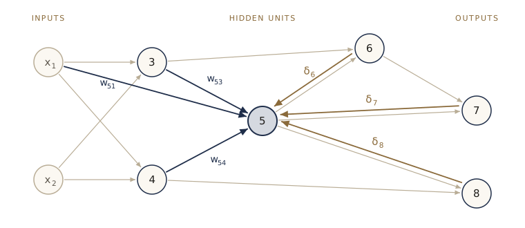
If different units use different activation functions, nothing changes except that each unit uses its own \(h'\). The next figure shows a small network with no layer structure, and the cell after it runs the four steps on exactly that network, unit by unit, with Python dictionaries so that the code mirrors the formulas.
# units 1 and 2 are the inputs; parents[j] lists the units that feed unit j
parents = {3: [1, 2], 4: [1, 2], 5: [1, 3, 4], 6: [3, 5], 7: [5, 6], 8: [4, 5]}
outputs = [7, 8]                               # linear outputs, sum-of-squares error
children = {i: [j for j in parents if i in parents[j]] for i in range(1, 9)}
w = {(j, i): rng.normal() for j in parents for i in parents[j]}     # w[j, i] = w_ji
bias = {j: 0.5 * rng.normal() for j in parents}

def dag_forward(x):
    """Forward propagation in topological order; returns the activations z_j."""
    z = {1: x[0], 2: x[1]}
    for j in sorted(parents):                  # 3, 4, ..., 8 is a topological order
        a_j = sum(w[j, i] * z[i] for i in parents[j]) + bias[j]
        z[j] = a_j if j in outputs else math.tanh(a_j)
    return z

def dag_backward(z, t):
    """Errors delta_j in reverse topological order, then dE/dw_ji = delta_j z_i."""
    delta = {}
    for j in sorted(parents, reverse=True):
        if j in outputs:
            delta[j] = z[j] - t[outputs.index(j)]                     # y_k - t_k
        else:                                                         # h'(a) = 1 - z^2
            delta[j] = (1 - z[j] ** 2) * sum(w[k, j] * delta[k] for k in children[j])
    grad_w = {(j, i): delta[j] * z[i] for (j, i) in w}
    return delta, grad_w, delta                # bias gradients equal the deltas

x_n, t_n = [0.7, -1.2], [0.5, -0.3]
z = dag_forward(x_n)
delta, grad_w, grad_b = dag_backward(z, t_n)
print("errors:", {j: round(d, 4) for j, d in sorted(delta.items())})

# the same network in PyTorch, differentiated by autograd
f64 = torch.float64
w_t = {key: torch.tensor(v, dtype=f64, requires_grad=True) for key, v in w.items()}
b_t = {j: torch.tensor(v, dtype=f64, requires_grad=True) for j, v in bias.items()}
zt = {1: torch.tensor(x_n[0], dtype=f64), 2: torch.tensor(x_n[1], dtype=f64)}
for j in sorted(parents):
    a_j = sum(w_t[j, i] * zt[i] for i in parents[j]) + b_t[j]
    zt[j] = a_j if j in outputs else torch.tanh(a_j)
E_t = 0.5 * sum((zt[k] - tk) ** 2 for k, tk in zip(outputs, t_n))
E_t.backward()
diff = max(max(abs(grad_w[key] - w_t[key].grad.item()) for key in w),
           max(abs(grad_b[j] - b_t[j].grad.item()) for j in bias))
print(f"{len(w) + len(bias)} parameters; largest difference from torch: {diff:.1e}")
errors: {3: 0.6498, 4: -0.0274, 5: 0.4008, 6: 0.0481, 7: -0.038, 8: -0.2057}
19 parameters; largest difference from torch: 1.1e-16
The errors come out in the order 8, 7, 6, …, 3, and each one uses only errors computed before it. The connections that skip levels need no special treatment: unit 5 takes an input directly from \(x_1\) and feeds an output directly, and the formula sums over whatever children a unit has.
Layered networks and mini-batches
Most networks in this course are organized in layers, and then the unit-by-unit formulas collapse into a few matrix operations. Write layer \(l\) as
\[\mathbf{a}^{(l)} = \mathbf{W}^{(l)} \mathbf{z}^{(l-1)} + \mathbf{b}^{(l)}, \qquad \mathbf{z}^{(l)} = h(\mathbf{a}^{(l)}),\]with \(\mathbf{z}^{(0)} = \mathbf{x}\) and \(\mathbf{W}^{(l)}\) of shape (units in layer \(l\)) × (units in layer \(l-1\)). The children of a unit in layer \(l\) are all the units of layer \(l+1\), so the backpropagation formula becomes
\[\boldsymbol{\delta}^{(l)} = h'(\mathbf{a}^{(l)}) \odot \left( \mathbf{W}^{(l+1)\mathrm{T}} \boldsymbol{\delta}^{(l+1)} \right), \qquad \frac{\partial E_n}{\partial \mathbf{W}^{(l)}} = \boldsymbol{\delta}^{(l)} \mathbf{z}^{(l-1)\mathrm{T}}, \qquad \frac{\partial E_n}{\partial \mathbf{b}^{(l)}} = \boldsymbol{\delta}^{(l)},\]where \(\odot\) is the elementwise product. The errors travel backward through the transposes of the weight matrices that carried the activations forward.
For a mini-batch we follow the PyTorch convention of one row per data point. Stack the activations as \(\mathbf{Z}^{(l)}\) (\(N \times\) width) and the errors as \(\boldsymbol{\Delta}^{(l)}\); then
\[\begin{aligned} \mathbf{A}^{(l)} &= \mathbf{Z}^{(l-1)} \mathbf{W}^{(l)\mathrm{T}} + \mathbf{b}^{(l)}, \\ \boldsymbol{\Delta}^{(l)} &= h'(\mathbf{A}^{(l)}) \odot \left( \boldsymbol{\Delta}^{(l+1)} \mathbf{W}^{(l+1)} \right), \\ \nabla_{\mathbf{W}^{(l)}} E &= \boldsymbol{\Delta}^{(l)\mathrm{T}} \mathbf{Z}^{(l-1)} , \end{aligned}\]and the bias gradient is the column sum of \(\boldsymbol{\Delta}^{(l)}\). The matrix product \(\boldsymbol{\Delta}^{(l)\mathrm{T}} \mathbf{Z}^{(l-1)}\) carries out the sum over the batch.
It pays to look at this one more way, because it is how every deep learning library is organized. Think of each piece of the network, a linear map, an elementwise nonlinearity, the error function, as a module with two methods. forward maps its input to its output and caches whatever it will need later. backward receives \(\partial E / \partial(\text{output})\) and returns \(\partial E / \partial(\text{input})\), storing the derivatives with respect to its own parameters on the way. If the module computes \(\mathbf{u} = f(\mathbf{v})\) with Jacobian \(\partial \mathbf{u} / \partial \mathbf{v}\), then backward computes
a vector–Jacobian product. It never forms the Jacobian itself: for an elementwise nonlinearity the product is an elementwise multiplication by \(h'\), and for a linear layer it is a multiplication by \(\mathbf{W}\). A network is a chain of modules, and backpropagation calls their backward methods in reverse order. In this language the \(\delta\)’s are just the incoming derivatives at the pre-activations.
Here is the whole library. Each module keeps its cached values in self.cache, and Linear stores its parameter gradients in dW and db. For the error functions we write two heads: a softmax cross-entropy, which (like PyTorch’s F.cross_entropy) averages over the mini-batch, so its output errors are \((\mathbf{Y} - \mathbf{T})/N\), and the sum-of-squares error with linear outputs, which sums, so its output errors are \(\mathbf{Y} - \mathbf{T}\).
class Module:
    """Base class: a module without parameters."""
    cache = None
    def params(self):
        return []
    def grads(self):
        return []

class Linear(Module):
    """A = Z W^T + b for a mini-batch Z of shape (N, d_in); W has shape (d_out, d_in)."""
    def __init__(self, d_in, d_out, rng, gain=1.0):
        self.W = rng.normal(0.0, math.sqrt(gain / d_in), (d_out, d_in))    # w_ji
        self.b = np.zeros(d_out)
    def forward(self, Z):
        self.cache = Z                     # the inputs z_i, needed for dE/dw_ji
        return Z @ self.W.T + self.b       # a_j = sum_i w_ji z_i + b_j
    def backward(self, Delta):             # Delta = dE/dA, shape (N, d_out)
        self.dW = Delta.T @ self.cache     # dE/dw_ji = sum_n delta_nj z_ni
        self.db = Delta.sum(axis=0)
        return Delta @ self.W              # dE/dz_i = sum_j w_ji delta_j
    def params(self):
        return [self.W, self.b]
    def grads(self):
        return [self.dW, self.db]

class Tanh(Module):
    def forward(self, A):
        self.cache = np.tanh(A)
        return self.cache
    def backward(self, G):                 # G = dE/dz
        return G * (1.0 - self.cache ** 2) # delta = h'(a) dE/dz with h'(a) = 1 - z^2

class ReLU(Module):
    def forward(self, A):
        self.cache = A > 0
        return A * self.cache
    def backward(self, G):
        return G * self.cache              # h'(a) = 1 for a > 0, else 0

class Softmax(Module):
    """Softmax as a separate module, used when we want probabilities as outputs."""
    def forward(self, A):
        self.cache = softmax(A)
        return self.cache
    def backward(self, G):                 # sum_k g_k y_k (I_kj - y_j), row by row
        Y = self.cache
        return Y * (G - (G * Y).sum(axis=1, keepdims=True))

class SoftmaxCrossEntropy:
    """Head: mean cross-entropy -(1/N) sum_n ln y_{n, t_n} from logits and integer labels."""
    def forward(self, A, t):
        logY = A - logsumexp(A, axis=1, keepdims=True)
        self.cache = (np.exp(logY), t)
        return -logY[np.arange(len(t)), t].mean()
    def backward(self):
        Y, t = self.cache
        return (Y - np.eye(Y.shape[1])[t]) / len(t)       # (y_k - t_k) / N

class SumOfSquares:
    """Head: E = (1/2) sum_n sum_k (y_nk - t_nk)^2 with linear outputs."""
    def forward(self, A, T):
        self.cache = A - T
        return 0.5 * np.sum(self.cache ** 2)
    def backward(self):
        return self.cache                                 # y_k - t_k

class Sequential(Module):
    def __init__(self, *layers):
        self.layers = list(layers)
    def forward(self, X):
        for layer in self.layers:
            X = layer.forward(X)
        return X
    def backward(self, Delta):
        for layer in reversed(self.layers):
            Delta = layer.backward(Delta)
        return Delta                       # dE/dx for every row of the input
    def params(self):
        return [p for layer in self.layers for p in layer.params()]
    def grads(self):
        return [g for layer in self.layers for g in layer.grads()]

def loss_and_grad(net, head, X, T):
    """Error and its gradient (a list of arrays shaped like net.params())."""
    E = head.forward(net.forward(X), T)
    net.backward(head.backward())
    return E, net.grads()
Optimizers, gradient checks, and Hessians all prefer the parameters as one flat vector \(\mathbf{w}\), so we add two helpers that copy between the list of arrays and a vector, and one that builds the same network in PyTorch with our weights copied in (PyTorch’s nn.Linear stores its weight as (out, in), like ours). The check uses a network with both kinds of hidden unit and a softmax cross-entropy head, in double precision.
def get_flat(net):
    return np.concatenate([p.ravel() for p in net.params()])

def set_flat(net, w):
    """Write the flat vector w into the network's parameter arrays, in place."""
    i = 0
    for p in net.params():
        p[...] = w[i:i + p.size].reshape(p.shape)
        i += p.size

def to_torch(net):
    """The same network in PyTorch (float64), with our weights copied in."""
    mods = []
    for layer in net.layers:
        if isinstance(layer, Linear):
            lin = torch.nn.Linear(layer.W.shape[1], layer.W.shape[0]).double()
            with torch.no_grad():
                lin.weight.copy_(torch.from_numpy(layer.W))
                lin.bias.copy_(torch.from_numpy(layer.b))
            mods.append(lin)
        else:
            mods.append(dict(Tanh=torch.nn.Tanh, ReLU=torch.nn.ReLU,
                             Softmax=lambda: torch.nn.Softmax(dim=1))[type(layer).__name__]())
    return torch.nn.Sequential(*mods)

def rel_error(a, b):
    """Largest componentwise relative difference between two arrays."""
    return np.max(np.abs(a - b) / np.maximum(np.abs(a) + np.abs(b), 1e-12))

net = Sequential(Linear(5, 8, rng), Tanh(), Linear(8, 6, rng, gain=2.0), ReLU(),
                 Linear(6, 3, rng))
head = SoftmaxCrossEntropy()
X = rng.normal(size=(16, 5))
t = rng.integers(0, 3, 16)
E, grads = loss_and_grad(net, head, X, t)
g_bp = np.concatenate([g.ravel() for g in grads])

tnet = to_torch(net)
E_t = F.cross_entropy(tnet(torch.from_numpy(X)), torch.from_numpy(t))
E_t.backward()
g_torch = torch.cat([p.grad.ravel() for p in tnet.parameters()]).numpy()
print(f"W = {g_bp.size} parameters, E = {E:.6f} (torch: {E_t.item():.6f})")
print(f"backprop vs torch.autograd: max relative error {rel_error(g_bp, g_torch):.1e}")
W = 123 parameters, E = 1.174043 (torch: 1.174043)
backprop vs torch.autograd: max relative error 7.6e-15
Our backward pass and PyTorch’s agree to about machine precision. PyTorch never saw our derivation; it differentiated the forward computation automatically. How it does that is the subject of the second half of this module.
A simple example
To see every number, take a two-layer network with \(D = 2\) inputs, \(M = 2\) tanh hidden units, \(K = 2\) linear outputs, and the sum-of-squares error for one data point. For tanh, \(h'(a) = 1 - \tanh^2(a) = 1 - z^2\), so the backward pass needs only the stored hidden activations. The equations are
\[\begin{aligned} a_j &= \sum_{i} w^{(1)}_{ji} x_i + b^{(1)}_j, & z_j &= \tanh(a_j), & y_k &= \sum_{j} w^{(2)}_{kj} z_j + b^{(2)}_k, \\ \delta_k &= y_k - t_k, & \delta_j &= (1 - z_j^2) \sum_{k} w^{(2)}_{kj} \delta_k, & \frac{\partial E_n}{\partial w^{(2)}_{kj}} &= \delta_k z_j, \quad \frac{\partial E_n}{\partial w^{(1)}_{ji}} = \delta_j x_i . \end{aligned}\]We pick small round weights so that each step can be followed with a calculator, and print the forward quantities, the errors, and the gradients in the order the algorithm produces them.
x = np.array([1.0, -2.0])
t_k = np.array([0.5, -0.5])
W1 = np.array([[0.2, -0.4], [0.7, 0.1]])     # w_ji^(1)
b1 = np.array([0.1, -0.2])
W2 = np.array([[0.6, -0.3], [-0.5, 0.8]])    # w_kj^(2)
b2 = np.array([0.0, 0.2])

a = W1 @ x + b1                  # forward
z = np.tanh(a)
y = W2 @ z + b2
E = 0.5 * np.sum((y - t_k) ** 2)
d_out = y - t_k                  # backward: output errors
d_hid = (1 - z ** 2) * (W2.T @ d_out)
print("a      =", a, "  z =", z)
print("y      =", y, f"  E = {E:.4f}")
print("delta_k =", d_out, "  delta_j =", d_hid)
print("dE/dW2 =\n", np.outer(d_out, z))
print("dE/dW1 =\n", np.outer(d_hid, x))

# the same network in our library, and in PyTorch
small = Sequential(Linear(2, 2, rng), Tanh(), Linear(2, 2, rng))
set_flat(small, np.concatenate([W1.ravel(), b1, W2.ravel(), b2]))
E_lib, g_lib = loss_and_grad(small, SumOfSquares(), x[None, :], t_k[None, :])
tsmall = to_torch(small)
(0.5 * ((tsmall(torch.from_numpy(x[None, :])) - torch.from_numpy(t_k)) ** 2).sum()).backward()
print("library dE/dW1 matches:", np.allclose(g_lib[0], np.outer(d_hid, x)),
      "  torch matches:", np.allclose(g_lib[0], tsmall[0].weight.grad.numpy()))
a      = [1.1 0.3]   z = [0.8005 0.2913]
y      = [0.3929 0.0328]   E = 0.1477
delta_k = [-0.1071  0.5328]   delta_j = [-0.1188  0.4195]
dE/dW2 =
 [[-0.0857 -0.0312]
 [ 0.4265  0.1552]]
dE/dW1 =
 [[-0.1188  0.2375]
 [ 0.4195 -0.8389]]
library dE/dW1 matches: True   torch matches: True
Follow one path through the numbers. Hidden unit \(j = 1\) has \(a_1 = 0.2 \cdot 1 - 0.4 \cdot (-2) + 0.1 = 1.1\) and \(z_1 = \tanh 1.1 = 0.8005\). The two outputs miss their targets by \(\delta_{k=1} = -0.1071\) and \(\delta_{k=2} = 0.5328\). Hidden unit 1 collects these errors through the weights it sends out, \(0.6 \cdot (-0.1071) - 0.5 \cdot 0.5328 = -0.3307\), and multiplies by its slope \(1 - z_1^2 = 0.3592\), which gives its error \(\delta_{j=1} = -0.1188\). The derivative with respect to the weight from \(x_2 = -2\) into that unit is then \(\delta_{j=1}\, x_2 = 0.2375\), the top-right entry of dE/dW1. The hand computation, the library, and PyTorch agree.
Numerical differentiation
Backpropagation’s great virtue is its cost. A forward pass costs \(O(W)\) operations for a network with \(W\) weights and biases: apart from very sparse networks, there are many more weights than units, so the weighted sums dominate, and each weight contributes one multiplication and one addition. The backward pass visits each weight twice more (once to pass errors back, once to form its derivative), so the complete gradient costs a small constant times the forward pass, still \(O(W)\).
The obvious alternative is to perturb each weight in turn and watch the error change. The forward difference
\[\frac{\partial E}{\partial w_i} \approx \frac{E(\mathbf{w} + \epsilon \mathbf{e}_i) - E(\mathbf{w})}{\epsilon},\]where \(\mathbf{e}_i\) is the \(i\)th unit vector, and the central difference
\[\frac{\partial E}{\partial w_i} \approx \frac{E(\mathbf{w} + \epsilon \mathbf{e}_i) - E(\mathbf{w} - \epsilon \mathbf{e}_i)}{2\epsilon}\]need only code for the forward pass. How accurate are they? Write \(E(w_i + \epsilon)\) for the error with only weight \(i\) perturbed and expand in a Taylor series:
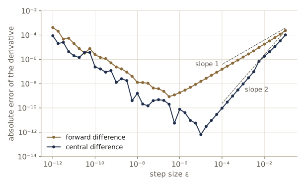
\[E(w_i \pm \epsilon) = E \pm \epsilon E' + \frac{\epsilon^2}{2} E'' \pm \frac{\epsilon^3}{6} E''' + O(\epsilon^4),\]with all derivatives taken with respect to \(w_i\) at the current point. Dividing \(E(w_i + \epsilon) - E\) by \(\epsilon\) leaves \(E' + \tfrac{\epsilon}{2} E'' + O(\epsilon^2)\): the forward difference has a truncation error of order \(\epsilon\). In the central difference the even powers cancel, leaving \(E' + \tfrac{\epsilon^2}{6} E''' + O(\epsilon^4)\), an error of order \(\epsilon^2\) for twice the work.
That argues for a tiny \(\epsilon\), but the computer disagrees. Each evaluation of \(E\) carries a relative round-off error of about the machine precision \(u\) (\(u \approx 1.1 \times 10^{-16}\) in double precision), so the numerator carries an absolute error of about \(u \lvert E \rvert\), and dividing by \(\epsilon\) amplifies it to about \(u \lvert E \rvert / \epsilon\). The total error of the central difference is therefore roughly
\[\frac{\epsilon^2}{6} \lvert E''' \rvert + \frac{u \lvert E \rvert}{\epsilon},\]which is smallest near \(\epsilon \approx (3 u \lvert E \rvert / \lvert E''' \rvert)^{1/3}\), around \(10^{-5}\) when the derivatives are of order one. The same reasoning for the forward difference balances \(\epsilon \lvert E'' \rvert / 2\) against \(2u \lvert E \rvert/\epsilon\) and gives an optimum near \(\sqrt{u} \approx 10^{-8}\). We test both predictions on one weight of the network from the gradient check, using the backpropagated derivative as the exact answer.
E_of = lambda v: (set_flat(net, v), head.forward(net.forward(X), t))[1]
w0 = get_flat(net)
i = 7                                          # one weight in the first layer
g_exact = g_bp[i]

def fd_errors(eps):
    e = np.zeros_like(w0)
    e[i] = eps
    forward_d = (E_of(w0 + e) - E_of(w0)) / eps
    central_d = (E_of(w0 + e) - E_of(w0 - e)) / (2 * eps)
    return abs(forward_d - g_exact), abs(central_d - g_exact)

eps_grid = np.logspace(-1, -12, 45)
errs = np.array([fd_errors(eps) for eps in eps_grid])
set_flat(net, w0)                              # restore the weights
for eps in [1e-1, 1e-3, 1e-5, 1e-7, 1e-9, 1e-11]:
    fe, ce = fd_errors(eps)
    print(f"eps = {eps:.0e}   forward error {fe:.1e}   central error {ce:.1e}")
set_flat(net, w0)
print(f"best eps: forward {eps_grid[errs[:, 0].argmin()]:.0e},"
      f" central {eps_grid[errs[:, 1].argmin()]:.0e}")
eps = 1e-01   forward error 2.4e-04   central error 1.0e-04
eps = 1e-03   forward error 1.5e-06   central error 9.5e-09
eps = 1e-05   forward error 1.5e-08   central error 6.4e-13
eps = 1e-07   forward error 3.8e-09   central error 4.8e-10
eps = 1e-09   forward error 2.3e-07   central error 1.3e-08
eps = 1e-11   forward error 2.0e-05   central error 2.0e-06
best eps: forward 3e-07, central 1e-05
Read the table from the top. Between \(\epsilon = 10^{-3}\) and \(10^{-5}\) the forward error falls by a factor of 100 (from \(1.5 \times 10^{-6}\) to \(1.5 \times 10^{-8}\)) and the central error by a factor of about \(10^4\) (from \(9.5 \times 10^{-9}\) to \(6.4 \times 10^{-13}\)): the orders \(\epsilon\) and \(\epsilon^2\) of the Taylor expansion. For smaller steps round-off takes over and both errors grow again. The best central step on the grid, \(10^{-5}\), matches the estimate. The best forward step, \(3 \times 10^{-7}\), lies above \(\sqrt{u} \approx 10^{-8}\) because the curvature along this weight is small: the truncation error at \(\epsilon = 10^{-3}\) implies \(\lvert E'' \rvert \approx 0.003\), and \(2\sqrt{u \lvert E \rvert / \lvert E'' \rvert}\) is then about \(4 \times 10^{-7}\). The figure shows the whole sweep.
Accuracy is only half of the problem; the other half is cost. Each finite-difference derivative needs one or two extra forward passes, and there are \(W\) weights, so a numerical gradient costs \(O(W)\) forward passes of \(O(W)\) operations each, \(O(W^2)\) in total, against \(O(W)\) for backpropagation. For a network with a million weights the difference is a factor of a million. The cell below times both on networks of growing width (your times will differ).
def best_time(f, repeats=3):
    """Shortest wall-clock time of f() over a few runs, in seconds."""
    times = []
    for _ in range(repeats):
        t0 = time.perf_counter()
        f()
        times.append(time.perf_counter() - t0)
    return min(times)

def numerical_gradient(E_of, w, eps=1e-6):
    """Central differences, one weight at a time: 2W evaluations of E."""
    g = np.zeros_like(w)
    for i in range(w.size):
        e = np.zeros_like(w)
        e[i] = eps
        g[i] = (E_of(w + e) - E_of(w - e)) / (2 * eps)
    return g

rng_t = np.random.default_rng(0)
X_t, t_t = rng_t.normal(size=(64, 20)), rng_t.integers(0, 5, 64)
for M in [10, 40, 160]:
    net_t = Sequential(Linear(20, M, rng_t), Tanh(), Linear(M, 5, rng_t))
    w_t = get_flat(net_t)
    E_t_of = lambda v: (set_flat(net_t, v), head.forward(net_t.forward(X_t), t_t))[1]
    t_bp = best_time(lambda: loss_and_grad(net_t, head, X_t, t_t), 20)
    t_fd = best_time(lambda: numerical_gradient(E_t_of, w_t), 1)
    set_flat(net_t, w_t)
    g_num = numerical_gradient(E_t_of, w_t)
    set_flat(net_t, w_t)
    g_back = np.concatenate([g.ravel() for g in loss_and_grad(net_t, head, X_t, t_t)[1]])
    print(f"W = {w_t.size:5d}   backprop {1e3 * t_bp:6.3f} ms   finite differences"
          f" {1e3 * t_fd:8.1f} ms   max relative error {rel_error(g_back, g_num):.0e}")
W =   265   backprop  0.271 ms   finite differences    202.3 ms   max relative error 6e-07
W =  1045   backprop  0.467 ms   finite differences    934.0 ms   max relative error 7e-07
W =  4165   backprop  0.386 ms   finite differences   3678.3 ms   max relative error 6e-06
The numerical gradients agree with backpropagation to about six significant digits in their worst component, but they cost hundreds to thousands of times more, and the gap widens with \(W\). The number of forward passes grows in proportion to \(W\). At these small sizes each pass costs about the same, because the fixed overhead of a few NumPy calls outweighs the arithmetic, so the finite-difference time here grows roughly linearly in \(W\); for a large network each pass also costs \(O(W)\) and the total grows like \(W^2\).
So finite differences are useless for training but invaluable for testing. Because they use only the forward code, they provide an independent check of any backward pass, hand-written or automatic.
In practice. Check every hand-written backward pass (a custom layer, a custom loss) against central differences before trusting it: double precision, a small network, a few data points, \(\epsilon\) around \(10^{-6}\), and the relative error per component. Values near \(10^{-7}\) or below mean agreement; a bug usually shows up as relative errors of order one in the affected components. PyTorch packages the same test as
torch.autograd.gradcheck.
Watch out. Two things make gradient checks fail when the code is right. In single precision (\(u \approx 6 \times 10^{-8}\)) the best attainable error is about \(10^{-5}\) times the scale of the error function, so run checks in float64. And ReLU and max-pooling have kinks: if a pre-activation lies within \(\epsilon\) of zero, the two perturbed evaluations fall on different linear pieces and the difference quotient is meaningless for that weight. A few isolated failures in a ReLU network are usually kinks, not bugs.
The Jacobian matrix
Backpropagation computes more than error gradients. The Jacobian matrix of a network collects the derivatives of its outputs with respect to its inputs,
\[J_{ki} = \frac{\partial y_k}{\partial x_i},\]each taken with the other inputs held fixed. Jacobians matter because networks are rarely used alone. Suppose a network with Jacobian \(\mathbf{J}\) takes its input \(\mathbf{z}\) from an earlier module with a parameter \(w\), and the error depends on the network’s outputs \(y_k\). Then
\[\frac{\partial E}{\partial w} = \sum_{k, j} \frac{\partial E}{\partial y_k} \frac{\partial y_k}{\partial z_j} \frac{\partial z_j}{\partial w},\]and the network’s Jacobian \(\partial y_k / \partial z_j\) sits in the middle, linking the error signal at its outputs to the module before it. This is exactly what Sequential.backward returns: \(\partial E / \partial \mathbf{x} = \mathbf{J}^{\mathrm{T}} (\partial E / \partial \mathbf{y})\), which the previous module can take as its own incoming error. The Jacobian also measures sensitivity: small input changes \(\Delta x_i\) change the outputs by \(\Delta y_k \approx \sum_i J_{ki} \Delta x_i\). Since the network is nonlinear, \(\mathbf{J}\) depends on \(\mathbf{x}\) and has to be recomputed at every input, and the linear estimate holds only for small changes.
To get the Jacobian itself, recall that one backward pass seeded with a vector \(\mathbf{u}\) at the outputs returns the vector–Jacobian product \(\mathbf{J}^{\mathrm{T}} \mathbf{u}\). Seeding with the unit vector \(\mathbf{e}_k\) gives row \(k\) of \(\mathbf{J}\), so the whole matrix takes \(K\) backward passes. Written out unit by unit, the pass for row \(k\) propagates \(\partial y_k / \partial a_j\) backward with the same recursion as the errors,
\[\frac{\partial y_k}{\partial a_j} = h'(a_j) \sum_{l \in \mathrm{ch}(j)} w_{lj} \frac{\partial y_k}{\partial a_l}, \qquad J_{ki} = \sum_{j \in \mathrm{ch}(i)} w_{ji} \frac{\partial y_k}{\partial a_j},\]starting at the outputs from the derivative of the output activation: \(I_{kl}\) for linear outputs (the identity matrix), \(I_{kl}\, \sigma'(a_l)\) for logistic-sigmoid outputs, and \(y_k (I_{kl} - y_l)\) for a softmax. In code the \(K\) passes can run as one batched pass: feed \(K\) copies of \(\mathbf{x}\) and seed the backward pass with the \(K \times K\) identity matrix, so that row \(k\) of the batch carries the seed \(\mathbf{e}_k\).
def jacobian_backprop(net, x, K):
    """J[k, i] = dy_k/dx_i at one input x: K backward passes, run as one batch."""
    net.forward(np.tile(x, (K, 1)))             # K identical rows
    return net.backward(np.eye(K))               # row k is seeded with e_k

net_j = Sequential(Linear(4, 6, rng), Tanh(), Linear(6, 3, rng), Softmax())
x0 = rng.normal(size=4)
J = jacobian_backprop(net_j, x0, 3)
tnet_j = to_torch(net_j)
J_torch = torch.autograd.functional.jacobian(lambda v: tnet_j(v[None, :])[0],
                                             torch.from_numpy(x0)).numpy()
print("Jacobian (3 outputs x 4 inputs):\n", J)
print(f"max relative error vs torch: {rel_error(J, J_torch):.1e}")
print("column sums:", J.sum(axis=0))
dx = 1e-3 * rng.normal(size=4)
dy = net_j.forward((x0 + dx)[None, :])[0] - net_j.forward(x0[None, :])[0]
print(f"output change {np.abs(dy).max():.2e}; error of the estimate J dx:"
      f" {np.abs(dy - J @ dx).max():.1e}")
Jacobian (3 outputs x 4 inputs):
 [[ 0.024  -0.0252  0.0264 -0.0322]
 [-0.0801  0.0219 -0.0382  0.129 ]
 [ 0.0562  0.0034  0.0118 -0.0968]]
max relative error vs torch: 1.9e-15
column sums: [ 0. -0.  0.  0.]
output change 6.39e-05; error of the estimate J dx: 2.2e-08
The backpropagated Jacobian matches PyTorch’s to round-off. Each column sums to zero (the printed \(-0.\) is a tiny negative round-off), as it must: softmax outputs always add up to one, so no change of input can change their total. And for a small random input change, \(\mathbf{J}\,\Delta\mathbf{x}\) predicts the change of the outputs (\(6.4 \times 10^{-5}\)) with an error of \(2.2 \times 10^{-8}\), more than three orders of magnitude smaller.
The Jacobian can also be built in the opposite direction, by pushing derivatives with respect to one input forward through the network alongside the activations; each such pass gives a column of \(\mathbf{J}\), so \(D\) passes give the matrix. That is forward-mode differentiation, and we meet it properly in the section on automatic differentiation, together with the question of when each direction is cheaper.
The Hessian matrix
Backpropagation can also deliver second derivatives. With all weights and biases collected into one vector \(\mathbf{w} = (w_1, \dots, w_W)\), the Hessian matrix has elements
\[H_{ij} = \frac{\partial^2 E}{\partial w_i \partial w_j} .\]It describes the local curvature of the error surface, which module 07 connects to the behavior of gradient descent. Second-order optimizers use it, the Laplace approximation of a Bayesian network needs it (Intro to ML, module 05 works through that case), and curvature information has been used to decide which weights can be pruned or stored at lower precision with the least damage.
The trouble is size. The Hessian has \(W^2\) entries, so for a network with a million weights it has \(10^{12}\), far too many to compute or store, and inverting it would cost \(O(W^3)\). For small networks it can be computed in \(O(W^2)\) operations per data point, the least possible for \(W^2\) numbers. Three routes lead there: extend backpropagation to second derivatives (for a two-layer network this is exercise 8.6 in Bishop & Bishop); take central differences of the backpropagated gradient, one weight at a time, which costs \(2W\) gradients of \(O(W)\) each; or let automatic differentiation differentiate the gradient code. We compare the last two on a tiny regression network, and look at the eigenvalues.
def hessian_fd(grad_of, w, eps=1e-5):
    """Hessian by central differences of the gradient: column i from two gradients."""
    H = np.zeros((w.size, w.size))
    for i in range(w.size):
        e = np.zeros_like(w)
        e[i] = eps
        H[:, i] = (grad_of(w + e) - grad_of(w - e)) / (2 * eps)
    return 0.5 * (H + H.T)                      # symmetrize away round-off

rng_h = np.random.default_rng(1)
X_h = rng_h.uniform(-2, 2, size=(30, 2))
T_h = (np.sin(X_h[:, :1]) * np.cos(X_h[:, 1:]) + 0.1 * rng_h.normal(size=(30, 1)))
net_h = Sequential(Linear(2, 3, rng_h), Tanh(), Linear(3, 1, rng_h))
sse = SumOfSquares()
shapes = [p.shape for p in net_h.params()]

def grad_h(w):
    set_flat(net_h, w)
    return np.concatenate([g.ravel() for g in loss_and_grad(net_h, sse, X_h, T_h)[1]])

def E_h_torch(w):
    """The same error written in PyTorch as a function of the flat vector w."""
    W1, b1, W2, b2 = torch.split(w, [math.prod(s) for s in shapes])
    Z = torch.tanh(torch.from_numpy(X_h) @ W1.reshape(shapes[0]).T + b1)
    return 0.5 * ((Z @ W2.reshape(shapes[2]).T + b2 - torch.from_numpy(T_h)) ** 2).sum()

w_init = get_flat(net_h)
H_fd = hessian_fd(grad_h, w_init)
H_exact = torch.autograd.functional.hessian(E_h_torch, torch.from_numpy(w_init)).numpy()
lam = np.linalg.eigvalsh(H_exact)
print(f"W = {w_init.size}; finite differences vs exact Hessian:"
      f" relative difference {np.linalg.norm(H_fd - H_exact) / np.linalg.norm(H_exact):.1e}")
print("eigenvalues at the random start:")
print(np.round(lam, 2))
off = H_exact - np.diag(np.diag(H_exact))
print(f"share of the Hessian (Frobenius norm) off the diagonal:"
      f" {np.linalg.norm(off) / np.linalg.norm(H_exact):.2f}")
W = 13; finite differences vs exact Hessian: relative difference 8.7e-11
eigenvalues at the random start:
[-40.16 -35.55 -22.62 -15.11  -0.9   -0.28   0.1    0.21   4.23  21.92
  35.43  36.96  51.16]
share of the Hessian (Frobenius norm) off the diagonal: 0.92
The two routes agree to about \(10^{-10}\), the accuracy of the finite differences. At the random starting weights the Hessian is far from positive definite: six of its thirteen eigenvalues are negative, the most negative about \(-40\), while the largest is about \(51\). The error surface curves up in some directions and down in others there, a saddle-like shape that is typical away from a minimum.
The last line bears on a cheap approximation. Keeping only the diagonal of \(\mathbf{H}\) needs \(O(W)\) storage and makes the inverse trivial, and with further approximations the diagonal itself can be propagated backward in \(O(W)\) operations. But Hessians of real networks are usually far from diagonal (here 92 percent of the matrix, measured in the Frobenius norm, lies off the diagonal), so a diagonal approximation should be treated as a computational convenience rather than a picture of the curvature.
The outer-product approximation
A more convincing approximation comes from the form of the error. For regression with one output and \(E = \tfrac12 \sum_n (y_n - t_n)^2\), differentiating twice with respect to \(\mathbf{w}\) gives
\[\mathbf{H} = \sum_{n=1}^{N} \nabla y_n \, \nabla y_n^{\mathrm{T}} + \sum_{n=1}^{N} (y_n - t_n) \nabla\nabla y_n .\]The second sum is weighted by the residuals. At a good fit the residuals are small. There is also a statistical reason to drop it: the function that minimizes a sum-of-squares error is the conditional mean of the target (module 04), so at the optimum the residuals behave like zero-mean noise, and if they are uncorrelated with the second derivatives \(\nabla\nabla y_n\) the sum averages toward zero. What remains is the outer-product or Levenberg–Marquardt approximation
\[\mathbf{H} \approx \sum_{n=1}^{N} \mathbf{b}_n \mathbf{b}_n^{\mathrm{T}}, \qquad \mathbf{b}_n = \nabla y_n = \nabla a_n,\]where the last equality holds because the output is linear. Each \(\mathbf{b}_n\) is one backward pass seeded with 1 at the output, and the outer products cost \(O(W^2)\). Unlike the exact Hessian, the approximation is always positive semidefinite. For a logistic-sigmoid output with the cross-entropy error the same argument gives \(\mathbf{H} \approx \sum_n y_n (1 - y_n) \mathbf{b}_n \mathbf{b}_n^{\mathrm{T}}\).
Both cases are instances of one pattern, the Gauss–Newton (or generalized Gauss–Newton) approximation. Write \(\mathbf{J}_n = \partial \mathbf{a}_n / \partial \mathbf{w}\) for the \(K \times W\) Jacobian of the output pre-activations with respect to the weights, and \(\mathbf{M}_n = \partial^2 E_n / \partial \mathbf{a}_n \partial \mathbf{a}_n^{\mathrm{T}}\) for the \(K \times K\) Hessian of the error with respect to those pre-activations. Dropping the terms that involve second derivatives of the network gives
\[\mathbf{H} \approx \sum_{n} \mathbf{J}_n^{\mathrm{T}} \mathbf{M}_n \mathbf{J}_n ,\]with \(\mathbf{M}_n = \mathbf{I}\) for sum-of-squares, \(y_n(1 - y_n)\) for a sigmoid with cross-entropy, and \(\operatorname{diag}(\mathbf{y}_n) - \mathbf{y}_n \mathbf{y}_n^{\mathrm{T}}\) for a softmax with cross-entropy. Each \(\mathbf{M}_n\) is positive semidefinite, so the approximation is too.
The approximation should be good only for a trained network. We compute it at the random starting weights and again after training the tiny network with gradient descent with momentum.
def output_grads(net, X):
    """Rows b_n = gradient of the single output a(x_n, w) with respect to w; shape (N, W)."""
    rows = []
    for x in X:
        net.forward(x[None, :])
        net.backward(np.ones((1, 1)))            # seed dE/da = 1 at the output
        rows.append(np.concatenate([g.ravel() for g in net.grads()]))
    return np.array(rows)

def fit_momentum(grad_of, w, steps, lr, mu=0.9):
    """Plain gradient descent with momentum on a flat parameter vector."""
    w, v = w.copy(), np.zeros_like(w)
    for _ in range(steps):
        v = mu * v + grad_of(w)
        w = w - lr * v
    return w

w_fit = fit_momentum(grad_h, w_init, 4000, lr=0.002)
H_fit = torch.autograd.functional.hessian(E_h_torch, torch.from_numpy(w_fit)).numpy()
for name, wv, Hv in [("random start", w_init, H_exact), ("trained", w_fit, H_fit)]:
    set_flat(net_h, wv)
    B = output_grads(net_h, X_h)
    H_gn = B.T @ B
    rmse = math.sqrt(2 * sse.forward(net_h.forward(X_h), T_h) / len(X_h))
    print(f"{name:12s}  RMS residual {rmse:.3f}   outer product vs exact:"
          f" relative difference {np.linalg.norm(H_gn - Hv) / np.linalg.norm(Hv):.1e}"
          f"   smallest eigenvalue exact {np.linalg.eigvalsh(Hv)[0]:+.1e},"
          f" approx {np.linalg.eigvalsh(H_gn)[0]:+.1e}")
random start  RMS residual 1.143   outer product vs exact: relative difference 8.7e-01   smallest eigenvalue exact -4.0e+01, approx +1.1e-06
trained       RMS residual 0.098   outer product vs exact: relative difference 6.5e-03   smallest eigenvalue exact +1.7e-02, approx +3.1e-03
At the random start the outer-product matrix is a poor stand-in: the residuals are large (RMS 1.14), so the neglected term is large and the relative difference is 0.87. The approximation is positive semidefinite by construction (its smallest eigenvalue is zero up to round-off), while the true Hessian has an eigenvalue near \(-40\). After training, with an RMS residual of 0.098, close to the noise level 0.1 we put into the targets, the difference drops to 0.65 percent and both matrices are positive definite.
The outer-product form also gives the inverse Hessian in a single pass through the data: adding one term \(\mathbf{b}_n \mathbf{b}_n^{\mathrm{T}}\) is a rank-one update, and the inverse of a rank-one update follows from the Woodbury identity in \(O(W^2)\) operations. Intro to ML, module 05 implements this sequential inverse, together with the Levenberg–Marquardt optimizer that the approximation is named after.
Hessian–vector products
Often we need not \(\mathbf{H}\) but its product with a vector, \(\mathbf{H}\mathbf{v}\). Conjugate-gradient and truncated-Newton solvers work only with such products, and so do methods that estimate the largest eigenvalues of the Hessian, the sharpness of a minimum. Forming \(\mathbf{H}\) first would cost \(O(W^2)\) time and memory for an answer of size \(W\). The key observation is that \(\mathbf{H}\mathbf{v}\) is a directional derivative of the gradient:
\[\mathbf{H}\mathbf{v} = \frac{\partial}{\partial \alpha} \nabla E(\mathbf{w} + \alpha \mathbf{v}) \Big\rvert_{\alpha = 0} = \nabla \left( \mathbf{v}^{\mathrm{T}} \nabla E(\mathbf{w}) \right).\]Each form gives an \(O(W)\) algorithm. The first can be approximated by differencing two backpropagated gradients, \(\{\nabla E(\mathbf{w} + \epsilon \mathbf{v}) - \nabla E(\mathbf{w} - \epsilon\mathbf{v})\}/(2\epsilon)\), or computed exactly by pushing the derivative along \(\mathbf{v}\) through every line of the forward and backward passes. That exact scheme is Pearlmutter’s R-operator, derived for a two-layer network in Intro to ML, module 05; in the language of the next section it is forward-mode differentiation applied to the backpropagation code, called forward-over-reverse. The second form says: compute the gradient in a way that can itself be differentiated, take its inner product with \(\mathbf{v}\), and backpropagate once more. That is double backpropagation, or reverse-over-reverse. PyTorch offers both.
v = rng.normal(size=w_fit.size)
Hv_exact = H_fit @ v
eps = 1e-5
Hv_fd = (grad_h(w_fit + eps * v) - grad_h(w_fit - eps * v)) / (2 * eps)   # NumPy

w_t = torch.tensor(w_fit, requires_grad=True)
v_t = torch.from_numpy(v)
g_t, = torch.autograd.grad(E_h_torch(w_t), w_t, create_graph=True)   # differentiable gradient
Hv_rr, = torch.autograd.grad(g_t @ v_t, w_t)                          # reverse-over-reverse
_, Hv_fr = jvp(grad(E_h_torch), (torch.from_numpy(w_fit),), (v_t,))  # forward-over-reverse
for name, Hv in [("gradient differences", Hv_fd), ("double backprop", Hv_rr.numpy()),
                 ("forward-over-reverse", Hv_fr.numpy())]:
    print(f"{name:21s} vs H v: max relative error {rel_error(Hv, Hv_exact):.1e}")
gradient differences  vs H v: max relative error 7.2e-09
double backprop       vs H v: max relative error 2.2e-15
forward-over-reverse  vs H v: max relative error 1.7e-15
All three agree with the explicit product. The two automatic-differentiation routes are exact to round-off; gradient differencing reaches the usual finite-difference accuracy of about \(10^{-8}\). None of them formed a \(W \times W\) matrix.
The payoff shows on a network that is too large for its Hessian. The next cell takes a network with about a quarter of a million weights, whose Hessian would need hundreds of gigabytes, and times a Hessian–vector product against a plain gradient (your times will differ).
big = torch.nn.Sequential(torch.nn.Linear(784, 300), torch.nn.Tanh(),
                          torch.nn.Linear(300, 10)).double()
params = {name: p.detach() for name, p in big.named_parameters()}
W_big = sum(p.numel() for p in params.values())
Xb, yb = torch.randn(128, 784, dtype=torch.float64), torch.randint(0, 10, (128,))
loss_of = lambda p: F.cross_entropy(functional_call(big, p, (Xb,)), yb)
tangent = {name: torch.randn_like(p) for name, p in params.items()}

t_grad = best_time(lambda: grad(loss_of)(params), 5)
t_hvp = best_time(lambda: jvp(grad(loss_of), (params,), (tangent,)), 5)
print(f"W = {W_big:,}; a full Hessian would take {8 * W_big ** 2 / 1e9:,.0f} GB in float64")
print(f"gradient {1e3 * t_grad:.1f} ms,  Hessian-vector product {1e3 * t_hvp:.1f} ms,"
      f"  ratio {t_hvp / t_grad:.1f}")
W = 238,510; a full Hessian would take 455 GB in float64
gradient 4.6 ms,  Hessian-vector product 22.5 ms,  ratio 4.9
A Hessian–vector product costs a few gradients (the printed ratio), not the \(W = 238{,}510\) gradient-sized passes the full Hessian would take, even if the memory for it existed. This is what makes curvature information usable in large networks: sharpness estimates, Newton-type steps solved by conjugate gradients, and the analysis of training dynamics all run on Hessian–vector products.
Automatic differentiation
Four ways to get a gradient
We now have the backward pass for a handful of layers, written by hand. That is how neural networks were trained for many years, and it works: carefully written backward code is fast and exact to machine precision. But every new layer or loss means a new derivation and new code, both easy to get wrong, and the backward code duplicates much of the forward code, so the two must be changed together whenever the model changes. That friction limits how quickly one can try out new architectures. There are three other ways to get derivatives.
Numerical differentiation needs only the forward code, but we have just seen that it is inexact and costs \(O(W^2)\). Its role is testing.
Symbolic differentiation has a computer-algebra system apply the rules of calculus to a formula and hand back a formula for the derivative. The result is exact, but formulas for derivatives can be far larger than the formula they came from, a problem called expression swell. The product rule is the culprit: the derivative of \(u(x) v(x)\) is \(u'(x) v(x) + u(x) v'(x)\), which mentions \(u\) and \(v\) twice each, and when \(u\) and \(v\) are themselves products the duplication compounds at every level. Symbolic differentiation also needs a closed-form expression, so it cannot handle programs with loops, branches, or recursion.
Automatic differentiation, also called algorithmic differentiation or autodiff, takes the code that evaluates a function and produces code, or runs a computation, that evaluates its derivatives exactly, reusing the intermediate values the function computes anyway. Because it works on the sequence of operations the program actually executes, it handles loops, branches, and function calls without difficulty. Automatic differentiation is a mature field that grew up largely in numerical computing, independently of neural networks; PyTorch’s autograd and JAX are implementations of it.
To see expression swell and its cure, we write a symbolic differentiator of a dozen lines. Expressions are nested tuples such as ("mul", a, b), and we differentiate the family
which a program computes with two operations per step. We count the size of each expression written out in full (as a tree) and the number of distinct subexpressions, which is the size of the computation if every repeated subexpression is computed once and reused.
def d(e):
    """Symbolic derivative with respect to x of an expression built from tuples."""
    op = e[0]
    if op == "x":
        return ("1",)
    if op == "mul":                               # product rule
        return ("add", ("mul", d(e[1]), e[2]), ("mul", e[1], d(e[2])))
    if op == "cos":                               # chain rule
        return ("mul", ("neg", ("sin", e[1])), d(e[1]))
    raise ValueError(op)

def tree_size(e):
    """Number of operations when the expression is written out in full."""
    return 1 + sum(tree_size(c) for c in e[1:])

def distinct(e, seen=None):
    """The set of distinct subexpressions: the size with every repeat computed once."""
    seen = set() if seen is None else seen
    if e not in seen:
        seen.add(e)
        for c in e[1:]:
            distinct(c, seen)
    return seen

f_k = ("x",)
for k in range(1, 11):
    if k in (2, 4, 6, 8, 10):
        df = d(f_k)
        print(f"k = {k:2d}   formula size: f {tree_size(f_k):5d}, f' {tree_size(df):6d}"
              f"    distinct subexpressions: f {len(distinct(f_k)):3d}, f' {len(distinct(df)):3d}")
    f_k = ("mul", f_k, ("cos", f_k))
k =  2   formula size: f     4, f'     12    distinct subexpressions: f   3, f'   9
k =  4   formula size: f    22, f'    123    distinct subexpressions: f   7, f'  25
k =  6   formula size: f    94, f'    783    distinct subexpressions: f  11, f'  41
k =  8   formula size: f   382, f'   4287    distinct subexpressions: f  15, f'  57
k = 10   formula size: f  1534, f'  21759    distinct subexpressions: f  19, f'  73
Written out in full, even \(f_k\) doubles in size at each step, because \(f_k\) appears twice in \(f_{k+1}\). Its derivative grows faster still, to 21,759 operations at \(k = 10\), fourteen times the size of \(f_{10}\). Yet the number of distinct subexpressions grows only linearly: 19 for \(f_{10}\) (two new ones per step) and 73 for its derivative. All of the swell comes from writing the same subexpressions out again and again. Automatic differentiation never writes a formula out. It works on the sequence of operations, in which each intermediate value is computed once and then reused, so the derivative costs a small constant multiple of the function.
Evaluation traces
Automatic differentiation starts from the observation that any program that computes a number, however complicated, executes a finite sequence of elementary operations: additions, multiplications, and functions such as \(\exp\), \(\sin\), and \(\tanh\) whose derivatives are known. Recording that sequence, with a new name for every intermediate result, gives an evaluation trace, also called a Wengert list. The trace is a directed acyclic graph, the computational graph, whose nodes are the intermediate values and whose edges point from each operation’s arguments (its parents) to its result.
Our running example is a function of two inputs,
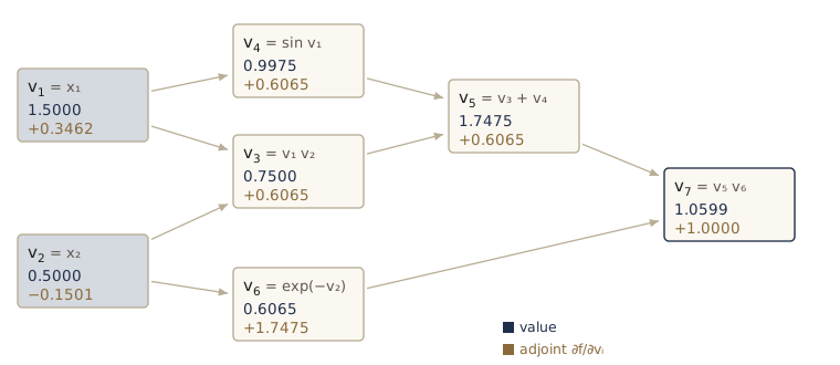
\[f(x_1, x_2) = \left( x_1 x_2 + \sin x_1 \right) e^{-x_2},\]whose trace, with the inputs as \(v_1\) and \(v_2\), is
\[\begin{aligned} v_1 &= x_1, & v_2 &= x_2, & v_3 &= v_1 v_2, & v_4 &= \sin v_1, \\ v_5 &= v_3 + v_4, & v_6 &= e^{-v_2}, & v_7 &= v_5 v_6, & f &= v_7 . \end{aligned}\]Both inputs are used twice: \(v_1\) feeds \(v_3\) and \(v_4\), and \(v_2\) feeds \(v_3\) and \(v_6\). Such fan-out is where naive symbolic differentiation duplicates work and where automatic differentiation must be careful to add up contributions. The figure shows the graph evaluated at \(x_1 = 1.5\), \(x_2 = 0.5\), and the cell computes the same numbers.
x1, x2 = 1.5, 0.5
v1 = x1                      # the primal trace, one elementary operation per line
v2 = x2
v3 = v1 * v2
v4 = math.sin(v1)
v5 = v3 + v4
v6 = math.exp(-v2)
v7 = v5 * v6
print("v1..v7 =", np.round([v1, v2, v3, v4, v5, v6, v7], 4))
df_dx1 = (x2 + math.cos(x1)) * math.exp(-x2)            # by hand, for reference
df_dx2 = (x1 - x1 * x2 - math.sin(x1)) * math.exp(-x2)
print(f"by hand: df/dx1 = {df_dx1:.6f}, df/dx2 = {df_dx2:.6f}")
v1..v7 = [1.5    0.5    0.75   0.9975 1.7475 0.6065 1.0599]
by hand: df/dx1 = 0.346170, df/dx2 = -0.150113
Forward-mode automatic differentiation
In forward mode we attach to every intermediate value \(v_i\), now called a primal variable, a second number \(\dot{v}_i\), its tangent: the derivative of \(v_i\) with respect to one chosen input, or more generally along one chosen direction in input space. The chain rule gives each tangent from the tangents of the node’s parents,
\[\dot{v}_i = \sum_{j \in \mathrm{pa}(i)} \frac{\partial v_i}{\partial v_j} \dot{v}_j ,\]where \(\mathrm{pa}(i)\) is the set of parents of node \(i\) and each local derivative \(\partial v_i / \partial v_j\) comes from one elementary operation. The tangents can therefore be computed in the same sweep as the primal values, in the same order. For \(\partial f / \partial x_1\) we seed \(\dot{v}_1 = 1\), \(\dot{v}_2 = 0\), and the trace becomes
\[\begin{aligned} \dot{v}_3 &= \dot{v}_1 v_2 + v_1 \dot{v}_2, & \dot{v}_4 &= \dot{v}_1 \cos v_1, & \dot{v}_5 &= \dot{v}_3 + \dot{v}_4, \\ \dot{v}_6 &= -\dot{v}_2\, e^{-v_2}, & \dot{v}_7 &= \dot{v}_5 v_6 + v_5 \dot{v}_6 . \end{aligned}\]The final tangent \(\dot{v}_7\) is \(\partial f / \partial x_1\). Each line needs only values already computed, so a primal value and its tangent can be discarded as soon as their children have used them.
A neat way to automate this uses dual numbers, numbers of the form \(a + b\varepsilon\) with the rule \(\varepsilon^2 = 0\). Arithmetic on them carries derivatives along by itself: \((a + b\varepsilon)(c + d\varepsilon) = ac + (ad + bc)\varepsilon\) is the product rule, and for a smooth function a Taylor expansion that stops after the linear term (all higher powers of \(\varepsilon\) vanish) gives \(g(a + b\varepsilon) = g(a) + g'(a)\, b\, \varepsilon\), the chain rule. So if we store the primal value in the real part and the tangent in the \(\varepsilon\) part, and teach each elementary operation these rules, any code built from those operations computes derivatives. In Python this is operator overloading. We write the elementary functions so that they also accept any object with an apply method; the reverse-mode engine below will plug into the same functions, so one definition of \(f\) serves floats, dual numbers, and graph nodes.
class Dual:
    """A dual number val + dot * eps with eps^2 = 0: a primal value and its tangent."""
    def __init__(self, val, dot=0.0):
        self.val, self.dot = float(val), float(dot)
    def apply(self, g, dg):                    # g(a + b eps) = g(a) + g'(a) b eps
        return Dual(g(self.val), dg(self.val) * self.dot)
    def __add__(self, o):
        o = o if isinstance(o, Dual) else Dual(o)
        return Dual(self.val + o.val, self.dot + o.dot)
    def __mul__(self, o):                      # (a + b eps)(c + d eps) = ac + (ad + bc) eps
        o = o if isinstance(o, Dual) else Dual(o)
        return Dual(self.val * o.val, self.dot * o.val + self.val * o.dot)
    def __truediv__(self, o):
        o = o if isinstance(o, Dual) else Dual(o)
        return Dual(self.val / o.val, (self.dot * o.val - self.val * o.dot) / o.val ** 2)
    def __pow__(self, p):                      # constant exponent p
        return Dual(self.val ** p, p * self.val ** (p - 1) * self.dot)
    def __neg__(self):
        return Dual(-self.val, -self.dot)
    def __sub__(self, o):
        return self + (-o)
    def __rsub__(self, o):
        return (-self) + o
    def __rtruediv__(self, o):
        return Dual(o) / self
    __radd__, __rmul__ = __add__, __mul__

def elementary(g, dg):
    """Lift g (with derivative dg) to floats and to any type with an apply method."""
    return lambda x: x.apply(g, dg) if hasattr(x, "apply") else g(x)

sin = elementary(math.sin, math.cos)
cos = elementary(math.cos, lambda a: -math.sin(a))
exp = elementary(math.exp, math.exp)
tanh = elementary(math.tanh, lambda a: 1.0 - math.tanh(a) ** 2)
softplus = elementary(lambda a: max(a, 0.0) + math.log1p(math.exp(-abs(a))),   # ln(1 + e^a)
                      lambda a: 1.0 / (1.0 + math.exp(-a)))                    # sigma(a)

def f(x1, x2):
    return (x1 * x2 + sin(x1)) * exp(-x2)

print(f"f(1.5, 0.5) = {f(1.5, 0.5):.6f}")
for seed in [(1.0, 0.0), (0.0, 1.0)]:        # one forward pass per input direction
    out = f(Dual(1.5, seed[0]), Dual(0.5, seed[1]))
    print(f"seed {seed}: primal {out.val:.6f}, tangent {out.dot:.6f}")
f(1.5, 0.5) = 1.059909
seed (1.0, 0.0): primal 1.059909, tangent 0.346170
seed (0.0, 1.0): primal 1.059909, tangent -0.150113
Each pass returns the value of \(f\) and one partial derivative, matching the hand-computed \(\partial f / \partial x_1\) and \(\partial f / \partial x_2\) above. For a function with \(D\) inputs, the full gradient takes \(D\) passes.
What does one pass give in general? For \(\mathbf{f}: \mathbb{R}^D \to \mathbb{R}^K\) with Jacobian \(\mathbf{J}\) (\(K \times D\)), seeding the input tangents with a vector \(\dot{\mathbf{x}} = \mathbf{r}\) produces output tangents \(\dot{\mathbf{f}} = \mathbf{J}\mathbf{r}\), a Jacobian–vector product, because the tangent recursion is linear in the seed. With \(\mathbf{r} = \mathbf{e}_i\) that is column \(i\) of \(\mathbf{J}\), for all \(K\) outputs at once. So forward mode builds the Jacobian one column per pass, and a directional derivative along any \(\mathbf{r}\) costs a single pass. We check both on a function with two outputs that share intermediate values, against PyTorch’s forward-mode tools torch.func.jvp and jacfwd.
def F2(x1, x2):
    """Two outputs that share the intermediate value u."""
    u = x1 * x2 + sin(x1)
    return [u * exp(-x2), u / (1 + x2 ** 2)]

def F2_torch(x):
    u = x[0] * x[1] + torch.sin(x[0])
    return torch.stack([u * torch.exp(-x[1]), u / (1 + x[1] ** 2)])

x_pt = torch.tensor([1.5, 0.5], dtype=torch.float64)
col_1 = [o.dot for o in F2(Dual(1.5, 1.0), Dual(0.5, 0.0))]      # J e_1: first column
r = (0.3, -1.2)
Jr = [o.dot for o in F2(Dual(1.5, r[0]), Dual(0.5, r[1]))]        # J r in one pass
J_t = jacfwd(F2_torch)(x_pt)
_, Jr_t = jvp(F2_torch, (x_pt,), (torch.tensor(r, dtype=torch.float64),))
print("column 1 of J:", np.round(col_1, 6), "  torch:", J_t[:, 0].numpy().round(6))
print("J r          :", np.round(Jr, 6), "  torch:", Jr_t.numpy().round(6))
column 1 of J: [0.3462 0.4566]   torch: [0.3462 0.4566]
J r          : [0.284  0.0391]   torch: [0.284  0.0391]
Because dual numbers ride along with whatever the program does, they differentiate straight through control flow. The next cell computes \(\sqrt{a}\) with a loop of Newton steps, \(y \leftarrow \tfrac12 (y + a/y)\), and asks for the derivative with respect to \(a\). There is no formula to differentiate, only an algorithm; the tangent follows the iteration and converges to \(1/(2\sqrt{a})\) along with the value.
def newton_sqrt(a, iters):
    y = a
    for _ in range(iters):
        y = 0.5 * (y + a / y)
    return y

for iters in [1, 2, 3, 5]:
    s = newton_sqrt(Dual(2.0, 1.0), iters)
    print(f"{iters} Newton steps: value {s.val:.10f}   derivative {s.dot:.10f}")
print(f"exact:          value {math.sqrt(2):.10f}   derivative {0.5 / math.sqrt(2):.10f}")
1 Newton steps: value 1.5000000000   derivative 0.5000000000
2 Newton steps: value 1.4166666667   derivative 0.3611111111
3 Newton steps: value 1.4142156863   derivative 0.3535659362
5 Newton steps: value 1.4142135624   derivative 0.3535533906
exact:          value 1.4142135624   derivative 0.3535533906
After five steps the value and the derivative agree with \(\sqrt{2}\) and \(1/(2\sqrt{2})\) to all printed digits. Strictly, forward mode returns the exact derivative of the function the program computes, here “five Newton steps starting from \(y = a\)”; that function converges to the square root, and its derivative converges to the derivative of the square root.
Reverse-mode automatic differentiation
Forward mode costs one pass per input. Training a network needs the derivatives of a single number, the error, with respect to millions of weights, and a million passes is hopeless. Reverse mode turns the computation around. It attaches to every intermediate value an adjoint
\[\bar{v}_i = \frac{\partial f}{\partial v_i},\]the sensitivity of the final output to that value. The output’s own adjoint is \(\bar{v}_{\text{out}} = 1\). Since \(v_i\) influences \(f\) only through its children, the nodes it is an argument of, the chain rule gives
\[\bar{v}_i = \sum_{j \in \mathrm{ch}(i)} \bar{v}_j \frac{\partial v_j}{\partial v_i} .\]This is the same recursion as backpropagation, with \(\delta_j\) generalized from pre-activations of units to arbitrary intermediate values: every \(\bar{v}_j\) on the right comes later in the trace, so the adjoints are computed in a reverse sweep after a complete forward sweep. For our \(f\):
\[\begin{aligned} \bar{v}_7 &= 1, & \bar{v}_6 &= \bar{v}_7 v_5, & \bar{v}_5 &= \bar{v}_7 v_6, & \bar{v}_4 &= \bar{v}_5, & \bar{v}_3 &= \bar{v}_5, \\ \bar{v}_2 &= \bar{v}_3 v_1 - \bar{v}_6 v_6, & \bar{v}_1 &= \bar{v}_3 v_2 + \bar{v}_4 \cos v_1 . \end{aligned}\]The last two lines each collect two terms, one per child: that is the fan-out of \(v_1\) and \(v_2\) at work. And one reverse sweep has produced both partial derivatives, \(\bar{v}_1 = \partial f / \partial x_1\) and \(\bar{v}_2 = \partial f / \partial x_2\). With a million inputs it would still be one sweep.
# forward sweep: primal and tangent (seed x1) together
t1, t2 = 1.0, 0.0
t3 = t1 * v2 + v1 * t2
t4 = t1 * math.cos(v1)
t5 = t3 + t4
t6 = -t2 * v6
t7 = t5 * v6 + v5 * t6
# reverse sweep: adjoints, after the primal trace is complete
a7 = 1.0
a6 = a7 * v5
a5 = a7 * v6
a4 = a5
a3 = a5
a2 = a3 * v1 - a6 * v6
a1 = a3 * v2 + a4 * math.cos(v1)
print(f"forward mode, seed x1: df/dx1 = {t7:.6f}")
print(f"reverse mode, one sweep: df/dx1 = {a1:.6f}, df/dx2 = {a2:.6f}")
print("adjoints a1..a7:", np.round([a1, a2, a3, a4, a5, a6, a7], 4))
forward mode, seed x1: df/dx1 = 0.346170
reverse mode, one sweep: df/dx1 = 0.346170, df/dx2 = -0.150113
adjoints a1..a7: [ 0.3462 -0.1501  0.6065  0.6065  0.6065  1.7475  1.    ]
Notice what the reverse sweep reads: \(v_1\), \(v_2\), \(v_5\), and \(v_6\), primal values from the forward sweep. Reverse mode must store the intermediate values of the forward sweep until the reverse sweep has used them, which forward mode never needs to do. We come back to that cost below.
A small autograd engine
To automate reverse mode we record the graph as the program runs. Our design: every scalar is a Value node that holds its number, its adjoint in grad, and a tuple of (parent, local derivative) pairs, where the local derivative \(\partial v_j / \partial v_i\) is computed during the forward sweep, while the numbers it needs are at hand. The reverse sweep then needs no knowledge of the operations at all. It orders the nodes so that every node comes after its parents (a topological sort, done here with an explicit stack so that deep graphs do not hit Python’s recursion limit), sets the output’s adjoint to 1, and walks the order backward, adding \(\bar{v}_j \cdot \partial v_j / \partial v_i\) into each parent’s adjoint. The += is where fan-out contributions are summed.
class Value:
    """A scalar node of a computational graph: its value, its adjoint (grad), and its
    parents with the local derivatives d(self)/d(parent)."""
    __slots__ = ("data", "grad", "parents")
    def __init__(self, data, parents=()):
        self.data, self.grad, self.parents = float(data), 0.0, parents
    def apply(self, g, dg):                    # elementary function: one parent
        return Value(g(self.data), ((self, dg(self.data)),))
    def __add__(self, o):
        o = o if isinstance(o, Value) else Value(o)
        return Value(self.data + o.data, ((self, 1.0), (o, 1.0)))
    def __mul__(self, o):
        o = o if isinstance(o, Value) else Value(o)
        return Value(self.data * o.data, ((self, o.data), (o, self.data)))
    def __truediv__(self, o):
        o = o if isinstance(o, Value) else Value(o)
        return Value(self.data / o.data,
                     ((self, 1.0 / o.data), (o, -self.data / o.data ** 2)))
    def __pow__(self, p):                      # constant exponent p
        return Value(self.data ** p, ((self, p * self.data ** (p - 1)),))
    def __neg__(self):
        return self * -1.0
    def __sub__(self, o):
        return self + (-o)
    def __rsub__(self, o):
        return (-self) + o
    def __rtruediv__(self, o):
        return Value(o) / self
    __radd__, __rmul__ = __add__, __mul__

    def backward(self):
        """Reverse sweep: fill in the adjoint of every node self depends on.
        Returns the number of nodes in the graph."""
        order, visited, stack = [], set(), [(self, False)]
        while stack:                           # depth-first search, parents first
            node, expanded = stack.pop()
            if expanded:
                order.append(node)
            elif id(node) not in visited:
                visited.add(id(node))
                stack.append((node, True))
                stack.extend((p, False) for p, _ in node.parents)
        for node in order:
            node.grad = 0.0
        self.grad = 1.0                        # d self / d self
        for node in reversed(order):           # every child before its parents
            for parent, local in node.parents:
                parent.grad += node.grad * local
        return len(order)

x1_v, x2_v = Value(1.5), Value(0.5)
out = f(x1_v, x2_v)                            # the same f as before
n_nodes = out.backward()
print(f"f = {out.data:.6f}; graph with {n_nodes} nodes;"
      f" df/dx1 = {x1_v.grad:.6f}, df/dx2 = {x2_v.grad:.6f}")
a_v = Value(2.0)
root = newton_sqrt(a_v, 5)                     # through the loop, in reverse mode
root.backward()
print(f"d sqrt(a)/da at a = 2 through 5 Newton steps: {a_v.grad:.10f}")
f = 1.059909; graph with 9 nodes; df/dx1 = 0.346170, df/dx2 = -0.150113
d sqrt(a)/da at a = 2 through 5 Newton steps: 0.3535533906
The engine reproduces the hand-written adjoints exactly, from the same definition of \(f\) that we fed to the dual numbers. The graph has 9 nodes rather than 7 because our engine records \(-x_2\) as a multiplication by the constant \(-1\), which adds the constant and the product as two nodes. Through the loop of Newton steps, reverse mode gives the same derivative as forward mode: the recorded graph is just the unrolled loop, one group of nodes per iteration.
Training a network with the engine
An engine that differentiates any scalar program can train a network, one scalar at a time. We build a tanh network with two hidden layers of 8 units whose weights are Value nodes, and use it to classify points from two noisy concentric rings in the plane, with the mean binary cross-entropy \(\frac{1}{N} \sum_n \{\ln(1 + e^{a_n}) - t_n a_n\}\) computed from the output pre-activation \(a_n\) (the softplus function above is \(\ln(1 + e^{a})\)). Before training, we check the engine’s gradient against PyTorch on the same weights.
def make_rings(N, rng):
    """Two noisy concentric rings: class 0 inside (radius 0.7), class 1 outside (1.5)."""
    t = rng.integers(0, 2, N)
    r = np.where(t == 1, 1.5, 0.7) + 0.25 * rng.normal(size=N)
    theta = rng.uniform(0, 2 * np.pi, N)
    return np.column_stack([r * np.cos(theta), r * np.sin(theta)]), t

class ValueMLP:
    """A tanh network whose weights are Value nodes, with one output pre-activation."""
    def __init__(self, sizes, rng):
        self.layers = []
        for d_in, d_out in zip(sizes[:-1], sizes[1:]):
            W = [[Value(rng.normal(0, 1 / math.sqrt(d_in))) for _ in range(d_in)]
                 for _ in range(d_out)]
            self.layers.append((W, [Value(0.0) for _ in range(d_out)]))
    def __call__(self, x):
        z = [float(x_i) for x_i in x]
        for l, (W, b) in enumerate(self.layers):
            a = [sum((w_ji * z_i for w_ji, z_i in zip(row, z)), b_j) for row, b_j in zip(W, b)]
            z = a if l == len(self.layers) - 1 else [tanh(a_j) for a_j in a]
        return z[0]
    def params(self):
        return [p for W, b in self.layers for p in [w for row in W for w in row] + b]

def bce(model, X, t):
    """Mean binary cross-entropy from the output pre-activations, as one Value."""
    total = Value(0.0)
    for x, t_n in zip(X, t):
        a = model(x)
        total = total + softplus(a) - float(t_n) * a
    return total * (1.0 / len(X))

rng_v = np.random.default_rng(3)
X_r, t_r = make_rings(100, rng_v)
model = ValueMLP([2, 8, 8, 1], rng_v)
E = bce(model, X_r, t_r)
n_nodes = E.backward()
g_engine = np.array([p.grad for p in model.params()])

tp = []                                        # the same weights as torch tensors
for W, b in model.layers:
    tp += [torch.tensor([[w.data for w in row] for row in W], dtype=torch.float64,
                        requires_grad=True),
           torch.tensor([b_j.data for b_j in b], dtype=torch.float64, requires_grad=True)]
Z_t = torch.from_numpy(X_r)
for l in range(0, len(tp), 2):
    Z_t = Z_t @ tp[l].T + tp[l + 1]
    Z_t = Z_t if l == len(tp) - 2 else torch.tanh(Z_t)
E_t = F.binary_cross_entropy_with_logits(Z_t[:, 0], torch.from_numpy(t_r).double())
E_t.backward()
g_torch = torch.cat([p.grad.ravel() for p in tp]).numpy()
print(f"{g_engine.size} weights; graph for 100 points: {n_nodes:,} nodes")
print(f"E = {E.data:.6f} (torch {E_t.item():.6f}); max relative error of the gradient"
      f" {rel_error(g_engine, g_torch):.1e}")
105 weights; graph for 100 points: 21,608 nodes
E = 0.813321 (torch 0.813321); max relative error of the gradient 7.0e-14
Now we train with mini-batches of 25 points and momentum, the same update rule as fit_momentum above, applied weight by weight.
params = model.params()
velocity = [0.0] * len(params)
lr, mu = 0.1, 0.9
t0 = time.perf_counter()
for epoch in range(1, 31):
    for idx in np.split(rng_v.permutation(len(X_r)), 4):
        E = bce(model, X_r[idx], t_r[idx])
        E.backward()
        for k, p in enumerate(params):
            velocity[k] = mu * velocity[k] + p.grad
            p.data -= lr * velocity[k]
    if epoch in (1, 5, 10, 20, 30):
        acc = np.mean([(model(x).data > 0) == t_n for x, t_n in zip(X_r, t_r)])
        print(f"epoch {epoch:2d}   training error {bce(model, X_r, t_r).data:.4f}"
              f"   accuracy {acc:.2f}")
print(f"120 steps in {time.perf_counter() - t0:.1f} s (your times will differ)")
epoch  1   training error 0.7230   accuracy 0.53
epoch  5   training error 0.6100   accuracy 0.69
epoch 10   training error 0.4429   accuracy 0.83
epoch 20   training error 0.1553   accuracy 0.96
epoch 30   training error 0.0763   accuracy 0.99
120 steps in 8.7 s (your times will differ)
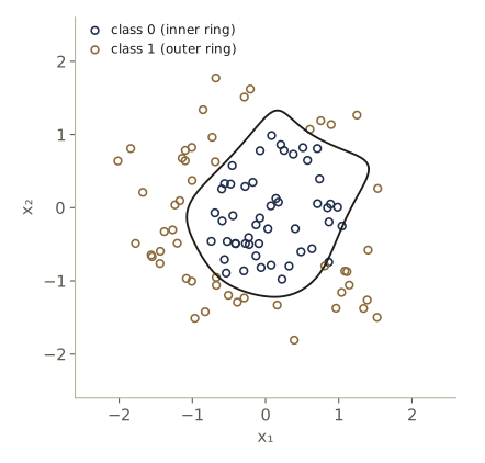
The engine’s gradient agrees with PyTorch’s to about \(10^{-13}\), relative. Training lowers the error from 0.72 to 0.076 over 30 epochs, and the network ends up classifying 99 of the 100 points correctly; the figure shows the closed boundary it found. The cost is also visible: the graph for one gradient over 100 points has 21,608 scalar nodes, and 120 small steps take several seconds.
Note. A scalar engine like ours is the whole idea of autograd in miniature; Andrej Karpathy’s
microgradis a well-known engine of the same kind, with a different design (each node stores a closure that runs its local backward step). PyTorch works the same way, but its nodes are tensor operations: each records a function that computes a vector–Jacobian product for a whole tensor, like thebackwardmethods of ourLinearandTanhmodules, and the graph for a mini-batch has a few dozen nodes instead of hundreds of thousands. That is the difference between the seconds our engine needs and the milliseconds PyTorch needs.
Forward or reverse mode?
Take a function \(\mathbf{f}: \mathbb{R}^D \to \mathbb{R}^K\) whose evaluation costs \(C\) operations. One forward-mode pass delivers one Jacobian–vector product \(\mathbf{J}\mathbf{r}\), a column of \(\mathbf{J}\) when \(\mathbf{r} = \mathbf{e}_i\). One reverse-mode sweep, seeded with \(\bar{\mathbf{f}} = \mathbf{u}\) at the outputs, delivers one vector–Jacobian product \(\mathbf{u}^{\mathrm{T}} \mathbf{J}\), a row of \(\mathbf{J}\) when \(\mathbf{u} = \mathbf{e}_k\). Either pass costs a small constant times \(C\) (Griewank and Walther’s book analyzes the constants; a factor of two or three over the function evaluation is typical). So the full Jacobian costs
\[\text{forward mode: } O(D \cdot C), \qquad \text{reverse mode: } O(K \cdot C).\]Forward mode wins when there are few inputs and many outputs; reverse mode wins when there are many inputs and few outputs. Training is the extreme case of the second: \(K = 1\) (the error) and \(D = W\) (the weights), so reverse mode gives the whole gradient for about the cost of one extra pass, while forward mode would need \(W\) passes, as bad as finite differences. That is why deep learning runs on reverse mode. Forward mode has its uses: directional derivatives, Jacobians of functions with few inputs, and, combined with reverse mode, the Hessian–vector products we computed earlier.
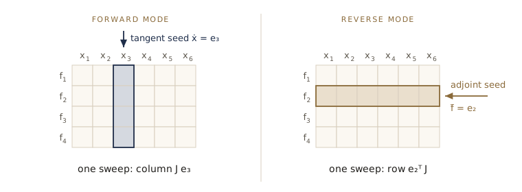
PyTorch exposes both directions as jacfwd and jacrev, which run all the passes at once as a batch. We time them on a small tanh network used in two shapes: many inputs and one output, and few inputs and many outputs (your times will differ).
def two_layer(A1, A2):
    return lambda x: A2 @ torch.tanh(A1 @ x)

dt = torch.float64
shapes_ad = {"R^1000 -> R^1": (1000, 1), "R^10 -> R^1000": (10, 1000)}
for name, (D_in, K_out) in shapes_ad.items():
    fn = two_layer(torch.randn(300, D_in, dtype=dt) / math.sqrt(D_in),
                   torch.randn(K_out, 300, dtype=dt) / math.sqrt(300))
    x_in = torch.randn(D_in, dtype=dt)
    same = torch.allclose(jacfwd(fn)(x_in), jacrev(fn)(x_in))
    t_fwd = best_time(lambda: jacfwd(fn)(x_in), 3)
    t_rev = best_time(lambda: jacrev(fn)(x_in), 3)
    print(f"{name:15s} Jacobian {K_out} x {D_in}: forward mode {1e3 * t_fwd:7.2f} ms,"
          f" reverse mode {1e3 * t_rev:7.2f} ms  (same result: {same})")
R^1000 -> R^1   Jacobian 1 x 1000: forward mode   15.17 ms, reverse mode    0.95 ms  (same result: True)
R^10 -> R^1000  Jacobian 1000 x 10: forward mode    1.81 ms, reverse mode   14.21 ms  (same result: True)
The two directions give the same Jacobian at very different cost. With a thousand inputs and one output, jacrev does one reverse sweep and is more than ten times faster than jacfwd, which runs a thousand tangent passes. With ten inputs and a thousand outputs the roles flip, and forward mode wins by a wide margin.
The memory cost of reverse mode
Reverse mode buys its speed with memory. The reverse sweep needs the primal values of the forward sweep (in our library, the cache of every module), so all of them must be kept until the backward pass reaches them. For a network, that means storing every layer’s activations for every example in the mini-batch. The parameters are stored once, but the activations scale with batch size times depth times width, and for large models they are usually what fills the accelerator’s memory. Forward mode does not have this problem: primal and tangent move forward together and can be discarded as soon as they are used.
Gradient checkpointing trades some of that memory back for computation. During the forward pass we keep only the inputs of a few segments of the network (the checkpoints) and throw the other cached values away. During the backward pass we rerun the forward computation of one segment at a time from its checkpoint, which restores that segment’s caches, and backpropagate through it. With \(L\) layers split into segments of about \(\sqrt{L}\) layers, memory falls from \(O(L)\) stored activations to \(O(\sqrt{L})\), at the price of roughly one extra forward pass. The cell implements this for our Sequential networks and counts the stored numbers (each distinct cached array is counted once).
def stored_numbers(arrays):
    """Total size of the distinct arrays in a list (shared arrays counted once)."""
    unique = dict((id(a), a) for a in arrays if a is not None)
    return sum(a.size for a in unique.values())

def grad_checkpointed(net, head, X, T, seg):
    """Backprop that keeps only every seg-th layer input during the forward pass.
    Returns the error and the peak number of stored values."""
    L = net.layers
    starts = list(range(0, len(L), seg))
    saved, peak, Z = [], 0, X
    for s in starts:                           # forward: keep only segment inputs
        saved.append(Z)
        for layer in L[s:s + seg]:
            Z = layer.forward(Z)
        peak = max(peak, stored_numbers(saved + [m.cache for m in L]))
        for layer in L[s:s + seg]:
            layer.cache = None                 # drop this segment's intermediate values
    E = head.forward(Z, T)
    Delta = head.backward()
    for s, Z in zip(reversed(starts), reversed(saved)):
        for layer in L[s:s + seg]:             # recompute this segment's caches
            Z = layer.forward(Z)
        peak = max(peak, stored_numbers(saved + [m.cache for m in L]))
        for layer in reversed(L[s:s + seg]):
            Delta = layer.backward(Delta)
            layer.cache = None
    return E, peak

rng_c = np.random.default_rng(4)
blocks = []
for _ in range(64):                            # 64 blocks of Linear(32, 32) + Tanh
    blocks += [Linear(32, 32, rng_c), Tanh()]
deep = Sequential(*blocks, Linear(32, 5, rng_c))
X_c, t_c = rng_c.normal(size=(128, 32)), rng_c.integers(0, 5, 128)

E_plain, g_plain = loss_and_grad(deep, head, X_c, t_c)
g_plain = [g.copy() for g in g_plain]
peak_plain = stored_numbers([m.cache for m in deep.layers])
for m in deep.layers:
    m.cache = None                             # start the checkpointed run from scratch
E_ckpt, peak_ckpt = grad_checkpointed(deep, head, X_c, t_c, seg=16)   # 8 blocks per segment
same = all(np.array_equal(a, b) for a, b in zip(g_plain, deep.grads()))
print(f"ordinary backprop: {peak_plain:,} stored values")
print(f"checkpointed:      {peak_ckpt:,} stored values at the peak;"
      f" identical gradients: {same}")
ordinary backprop: 266,240 stored values
checkpointed:      69,632 stored values at the peak; identical gradients: True
Ordinary backpropagation holds 65 activation arrays of \(128 \times 32\) numbers (the input batch and the outputs of the 64 tanh layers), 266,240 values. With segments of 8 blocks, the peak is 17 arrays: the saved inputs of the 9 segments (the last segment is the output layer alone) and the 8 tanh outputs of the segment being recomputed, about a quarter of the memory. The gradients are bit-for-bit identical, and the price is one extra forward pass through the network. In general, with \(L\) blocks and segments of \(s\) blocks the peak is about \(L/s + s\) arrays, which is smallest for \(s = \sqrt{L}\).
In practice. PyTorch provides checkpointing as
torch.utils.checkpoint; wrapping a block of a model in it makes autograd store only the block’s input and recompute the rest during the backward pass. It is a standard tool for fitting large models or long sequences into GPU memory, and the gradients it produces are the same as without it.
Training the from-scratch network on MNIST
We end where practice begins: training a real classifier with the NumPy library from the first half of the module. The network maps the \(28 \times 28 = 784\) pixel values of an MNIST digit through two ReLU hidden layers of 128 and 64 units to 10 logits, with the softmax cross-entropy head. The hidden layers use the initialization variance \(2/d_{\text{in}}\) suited to ReLU units (module 07 discusses initialization), and the optimizer is stochastic gradient descent with momentum, written in PyTorch’s convention \(\mathbf{v} \leftarrow \mu \mathbf{v} + \nabla E\), \(\mathbf{w} \leftarrow \mathbf{w} - \eta \mathbf{v}\) so that we can compare with torch.optim.SGD. To keep the run short on a CPU, we use the first 10,000 training images and the first 2,000 test images.
from torchvision import datasets
train = datasets.MNIST(root="data", train=True, download=True)
test = datasets.MNIST(root="data", train=False, download=True)
X_train = train.data[:10000].float().div(255.).reshape(-1, 784).double().numpy()
t_train = train.targets[:10000].numpy()
X_test = test.data[:2000].float().div(255.).reshape(-1, 784).double().numpy()
t_test = test.targets[:2000].numpy()

def mnist_net(rng):
    return Sequential(Linear(784, 128, rng, gain=2.0), ReLU(),
                      Linear(128, 64, rng, gain=2.0), ReLU(), Linear(64, 10, rng))

def sgd_momentum_step(params, grads, velocity, lr, mu=0.9):
    """v <- mu v + g, w <- w - lr v for every parameter array, in place."""
    for p, g, v in zip(params, grads, velocity):
        v *= mu
        v += g
        p -= lr * v

print("training images", X_train.shape, " test images", X_test.shape,
      f" parameters {get_flat(mnist_net(np.random.default_rng(0))).size:,}")
training images (10000, 784) test images (2000, 784) parameters 109,386
First, the promised check. We copy a freshly initialized network into PyTorch, compute the error and gradient on one mini-batch of 64 images in both, and take one momentum step in both.
net_m = mnist_net(np.random.default_rng(0))
tnet_m = to_torch(net_m)
xb, tb = X_train[:64], t_train[:64]
E, grads = loss_and_grad(net_m, head, xb, tb)
velocity = [np.zeros_like(p) for p in net_m.params()]
sgd_momentum_step(net_m.params(), grads, velocity, lr=0.05)

opt = torch.optim.SGD(tnet_m.parameters(), lr=0.05, momentum=0.9)
E_t = F.cross_entropy(tnet_m(torch.from_numpy(xb)), torch.from_numpy(tb))
opt.zero_grad()
E_t.backward()
grad_diff = max(np.abs(g - p.grad.numpy()).max() for g, p in zip(grads, tnet_m.parameters()))
opt.step()
weight_diff = max(np.abs(p - q.detach().numpy()).max()
                  for p, q in zip(net_m.params(), tnet_m.parameters()))
print(f"error: ours {E:.10f}, torch {E_t.item():.10f}")
print(f"largest gradient difference {grad_diff:.1e}; after one step, largest weight"
      f" difference {weight_diff:.1e}")
error: ours 2.3552318310, torch 2.3552318310
largest gradient difference 2.8e-17; after one step, largest weight difference 2.8e-17
The two implementations agree to round-off in the error, in every gradient component, and in the updated weights. Now we train for eight epochs with mini-batches of 64.
def accuracy(net, X, t):
    return np.mean(net.forward(X).argmax(axis=1) == t)

rng_m = np.random.default_rng(1)
net_m = mnist_net(rng_m)
velocity = [np.zeros_like(p) for p in net_m.params()]
losses = []
t0 = time.perf_counter()
for epoch in range(1, 9):
    for idx in np.array_split(rng_m.permutation(len(X_train)), len(X_train) // 64):
        E, grads = loss_and_grad(net_m, head, X_train[idx], t_train[idx])
        sgd_momentum_step(net_m.params(), grads, velocity, lr=0.05)
        losses.append(E)
    if epoch in (1, 2, 4, 6, 8):
        print(f"epoch {epoch}   mean training error (last epoch) {np.mean(losses[-156:]):.4f}"
              f"   train accuracy {accuracy(net_m, X_train, t_train):.4f}"
              f"   test accuracy {accuracy(net_m, X_test, t_test):.4f}")
print(f"{len(losses)} steps in {time.perf_counter() - t0:.1f} s (your times will differ)")
epoch 1   mean training error (last epoch) 0.5497   train accuracy 0.9385   test accuracy 0.8920
epoch 2   mean training error (last epoch) 0.2246   train accuracy 0.9575   test accuracy 0.9120
epoch 4   mean training error (last epoch) 0.0975   train accuracy 0.9807   test accuracy 0.9345
epoch 6   mean training error (last epoch) 0.0418   train accuracy 0.9855   test accuracy 0.9330
epoch 8   mean training error (last epoch) 0.0205   train accuracy 0.9981   test accuracy 0.9390
1248 steps in 3.8 s (your times will differ)
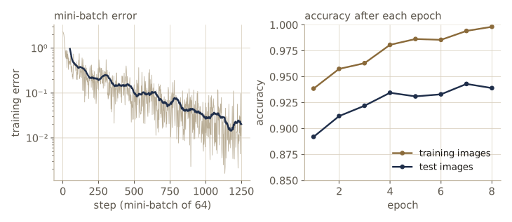
After eight epochs the network classifies 99.8 percent of its training images and 93.9 percent of the held-out test images correctly, and the whole run takes a few seconds on one CPU thread. The gap between the two numbers is overfitting: 109,386 parameters, 10,000 images, and no regularization. Training on all 60,000 images for more epochs, and adding the regularization methods of module 09, would raise the test accuracy; on a GPU one would also switch to single precision, since double precision is needed here only for the exact comparison with PyTorch. Nothing in the training loop depends on how the gradient was obtained: replace our modules by torch.nn ones and loss_and_grad by loss.backward(), and it becomes the training loop of module 07.
Finally, the claim that a gradient costs only a small multiple of a function evaluation, measured on this network with a mini-batch of 256 images (your times will differ).
xb, tb = X_train[:256], t_train[:256]
t_fwd = best_time(lambda: head.forward(net_m.forward(xb), tb), 20)
t_both = best_time(lambda: loss_and_grad(net_m, head, xb, tb), 20)
print(f"forward pass {1e3 * t_fwd:.2f} ms, forward + backward {1e3 * t_both:.2f} ms,"
      f" ratio {t_both / t_fwd:.1f}")
forward pass 2.99 ms, forward + backward 7.05 ms, ratio 2.4
The backward pass costs a small multiple of the forward pass, as the counting argument predicts. Each Linear module’s backward pass performs two matrix products the size of its single forward product, one for the weight gradient and one for the errors passed down, so we expect the two together to cost two to three times the forward pass alone; on a shared machine individual timings scatter around that. That is the practical meaning of \(O(W)\): a training step costs a few forward passes, however many parameters the network has.
Summary
| Method | What one pass computes | Cost | Key formula |
|---|---|---|---|
| Backpropagation | gradient of one error with respect to all \(W\) weights | \(O(W)\), a few forward passes | \(\delta_j = h'(a_j) \sum_k w_{kj} \delta_k\), \(\partial E_n / \partial w_{ji} = \delta_j z_i\) |
| Central differences | one derivative from two forward passes | \(O(W^2)\) for a gradient | error about \(\epsilon^2 \lvert E''' \rvert / 6 + u \lvert E \rvert / \epsilon\) |
| Jacobian by backpropagation | one row of \(\mathbf{J}\) per backward pass | \(K\) passes | \(J_{ki} = \sum_j w_{ji}\, \partial y_k / \partial a_j\) |
| Exact Hessian | all second derivatives | \(O(W^2)\) per data point | finite differences of gradients, or autodiff of the gradient |
| Outer-product (Gauss–Newton) | positive semidefinite curvature | \(O(W^2)\) | \(\mathbf{H} \approx \sum_n \mathbf{J}_n^{\mathrm{T}} \mathbf{M}_n \mathbf{J}_n\) |
| Hessian–vector product | \(\mathbf{H}\mathbf{v}\) | \(O(W)\), a few gradients | forward-over-reverse or double backprop |
| Forward-mode autodiff | Jacobian–vector product \(\mathbf{J}\mathbf{r}\) | one pass per input direction | \(\dot{v}_i = \sum_{j \in \mathrm{pa}(i)} (\partial v_i / \partial v_j)\, \dot{v}_j\) |
| Reverse-mode autodiff | vector–Jacobian product \(\mathbf{u}^{\mathrm{T}}\mathbf{J}\) | one sweep per output; stores the trace | \(\bar{v}_i = \sum_{j \in \mathrm{ch}(i)} \bar{v}_j\, \partial v_j / \partial v_i\) |
| Gradient checkpointing | the same gradient with less memory | one extra forward pass | memory \(O(\sqrt{L})\) instead of \(O(L)\) |
Ideas to carry forward:
- A network is a composition of modules, and each module needs only two things: a forward computation and a vector–Jacobian product. Backpropagation is reverse-mode automatic differentiation applied to that composition, and it is what
loss.backward()runs. The attention layers, message-passing layers, and invertible layers of later modules are differentiated the same way, without anyone deriving their gradients by hand. - A gradient costs a small constant times one evaluation of the error, whatever the number of weights. That fact, not any particular optimizer, is what makes training networks with millions of parameters possible.
- Reverse mode pays in memory: every activation needed by the backward pass is stored, so memory grows with batch size, depth, and width. Checkpointing trades recomputation for memory.
- Curvature is available cheaply as Hessian–vector products even when the Hessian itself is far too large to form. And finite differences remain the tool for checking any gradient code you write.
Exercises
- In a general feed-forward network an output unit may also feed other units (for example, an auxiliary output in the middle of a deep network). Show that its error is then the sum of the direct term \(\partial E_n / \partial a_j\) from the error function and the usual backpropagated term \(h'(a_j) \sum_k w_{kj} \delta_k\). Extend
dag_forwardanddag_backwardto allow unit 5 to be an extra linear output with its own target, and check the gradient against PyTorch. - Add a
Sigmoidmodule and aBinaryCrossEntropyhead (computed from the pre-activations, withnp.logaddexpfor stability) to the library. Derive theirbackwardmethods, show that the head’s output errors are \((y_n - t_n)/N\) for a mean over the batch, and check a small network againstF.binary_cross_entropy_with_logits. - A residual block computes \(\mathbf{z} + \mathbf{g}(\mathbf{z})\), where \(\mathbf{g}\) is some sub-network. Show that its vector–Jacobian product is \(\mathbf{u} + (\partial \mathbf{g} / \partial \mathbf{z})^{\mathrm{T}} \mathbf{u}\). Write a module
Residual(inner)whosebackwardimplements this, build a deep network of residual blocks, and check it against PyTorch. Then compare the size of \(\partial E / \partial \mathbf{x}\) in a deep plain network and in a deep residual network at initialization, and explain the difference from the backward formula. - The complex-step derivative of a real-analytic function is \(f'(x) \approx \operatorname{Im} f(x + i\epsilon) / \epsilon\). Use a Taylor expansion to show that its error is \(O(\epsilon^2)\) and that it involves no subtraction of nearly equal numbers. Apply it to one weight of a
Linear–Tanh–Linearnetwork with theSumOfSquareshead (the modules work unchanged if the weights are stored as complex arrays), and plot its error against \(\epsilon\) from \(10^{-1}\) down to \(10^{-20}\) next to the central difference. - Derive the optimal step sizes for the forward and central differences from the error models in the section on numerical differentiation, including the constants. Estimate \(E''\) and \(E'''\) for the weight used in the note from the truncation branches of the sweep, and compare the predicted optima with the observed ones.
- Give each module a method
jvp(self, dZ)that maps a tangent of its input to a tangent of its output, using the values cached inforward(forLinear, \(\dot{\mathbf{A}} = \dot{\mathbf{Z}} \mathbf{W}^{\mathrm{T}}\)). Use it to build the Jacobian ofnet_jcolumn by column in forward mode and compare withjacobian_backprop. For which shapes of network is each version cheaper? - For a softmax output with the cross-entropy error, show that \(\partial^2 E_n / \partial \mathbf{a} \partial \mathbf{a}^{\mathrm{T}} = \operatorname{diag}(\mathbf{y}_n) - \mathbf{y}_n \mathbf{y}_n^{\mathrm{T}}\) and that this matrix is positive semidefinite. Implement the Gauss–Newton approximation \(\sum_n \mathbf{J}_n^{\mathrm{T}} \mathbf{M}_n \mathbf{J}_n\) for a small classifier and compare it with the exact Hessian from
torch.autograd.functional.hessian, before and after training. - Use Hessian–vector products (forward-over-reverse) and power iteration, \(\mathbf{v} \leftarrow \mathbf{H}\mathbf{v} / \lVert \mathbf{H}\mathbf{v} \rVert\), to estimate the largest eigenvalue of the Hessian of the tiny regression network at
w_fit, and compare witheigvalsh. On a quadratic error, gradient descent is stable only for learning rates below \(2/\lambda_{\max}\); check this nearw_fitby running gradient descent just below and just above that rate. - Generalize
Dualso that its value and tangent may themselves beDualnumbers (drop thefloatconversions, and make the elementary functions call the lifted versions of their derivatives). Nest two levels to compute \(\partial^2 f / \partial x_1^2\) for the running example \(f\), and check against a formula you derive by hand. Which mode of differentiation have you built? - In
Value.backward, replaceparent.grad += node.grad * localbyparent.grad = node.grad * local. Before running anything, use the adjoint trace of \(f\) to predict which of \(\partial f / \partial x_1\) and \(\partial f / \partial x_2\) come out wrong and what values you will get. Then run it and explain the result in terms of fan-out. - Show that with \(L\) blocks and checkpoints every \(s\) blocks the peak number of stored activation arrays is about \(L/s + s\), and that the optimum \(s = \sqrt{L}\) gives about \(2\sqrt{L}\). Now apply checkpointing recursively inside each segment. Argue that memory can be reduced to \(O(\log L)\) arrays, and estimate how many forward passes this costs.
- In your own words: explain to a classmate who has only ever called
loss.backward()what happens during that call, why deep learning uses reverse mode rather than forward mode, and what reverse mode costs in memory.
Going further
- Bishop & Bishop, Deep Learning: Foundations and Concepts, chapter 8. Exercise 8.6 derives the exact Hessian of a two-layer network, 8.12 the one-pass inverse of the outer-product Hessian, and 8.13–8.18 work through expression swell, evaluation traces in forward and reverse mode, and Jacobian–vector products for the book’s own example function.
- D. E. Rumelhart, G. E. Hinton, and R. J. Williams, “Learning representations by back-propagating errors”, Nature 323 (1986), doi:10.1038/323533a0: the paper that made backpropagation the standard way to train multilayer networks.
- A. G. Baydin, B. A. Pearlmutter, A. A. Radul, and J. M. Siskind, “Automatic differentiation in machine learning: a survey”, Journal of Machine Learning Research 18 (2018), arXiv:1502.05767: a readable overview of forward and reverse mode, dual numbers, and implementation techniques.
- A. Griewank and A. Walther, Evaluating Derivatives: Principles and Techniques of Algorithmic Differentiation, 2nd ed., SIAM (2008): the standard reference on automatic differentiation, including cost bounds and checkpointing. For checkpointing in deep learning specifically, see T. Chen, B. Xu, C. Zhang, and C. Guestrin, “Training deep nets with sublinear memory cost” (2016), arXiv:1604.06174. B. A. Pearlmutter, “Fast exact multiplication by the Hessian”, Neural Computation 6 (1994), introduced the R-operator.
- On this site: Intro to ML, module 05 for the two-layer derivation, the diagonal Hessian recursion, the sequential inverse Hessian, the R-operator, and Levenberg–Marquardt; module 07 for the optimizers that consume these gradients; and EAS 510, module 01 for the PyTorch training loop in which
loss.backward()is called.
These notes follow the chapters of C. M. Bishop and H. Bishop, Deep Learning: Foundations and Concepts (Springer, 2024), the course text, which the authors make free to read online. The explanations, code, figures, and exercises here are written for this course; the book remains the reference, with the full derivations and many more exercises.