EAS 510 · Module 01 · Week 2
The PyTorch Workflow
The six steps of every project — data, model, loss, optimizer, training loop, evaluation — on a straight-line example.
Companion reading: Learn PyTorch for Deep Learning, chapter 01
By the end of this module you can
- Describe the six steps of a PyTorch project and say what each one produces.
- Create a dataset from a known formula and split it into training and test sets, and explain why a model must be tested on data it has not seen.
- Build a model as a subclass of
nn.Modulewith learnablenn.Parameters and aforwardmethod, and inspect it withstate_dict(). - Explain in plain language how a loss function, gradients, and an optimizer work together to improve a model.
- Write a training loop and a testing loop from memory, and explain every line — including
train(),eval(), andzero_grad(). - Read a loss curve, and save and reload a trained model with its
state_dict. - Rebuild the whole workflow with
nn.Linearin device-agnostic code.
Contents
- The workflow at a glance
- Step 1: Data
- Step 2: Building a model
- Step 3: A loss function and an optimizer
- Step 4: The training loop
- Step 5: Making predictions with a trained model
- Step 6: Saving and loading a model
- Putting it all together
- Summary
- Exercises
- Going further
In module 00 you met the tensor and saw that a neural network starts as random numbers that are gradually improved. This module shows how that improvement happens, from start to finish, on the smallest problem we could find: fitting a straight line.
A straight line is a deliberately easy target. Because we will make the data ourselves from a formula we know, we can check at every step whether the model is learning the right thing. The point is not the line; it is the workflow — the same six steps you will follow in every later module, whether the data is a spreadsheet, a photograph, or a sentence.
The workflow at a glance
Every PyTorch project, large or small, moves through the same steps:
| Step | What happens | What you end up with |
|---|---|---|
| 1. Data | Turn the data into tensors and split it into training and test sets | X_train, y_train, X_test, y_test |
| 2. Model | Define a model with learnable parameters | a model that makes (bad) predictions |
| 3. Loss and optimizer | Choose how to measure error and how to reduce it | loss_fn, optimizer |
| 4. Training loop | Repeatedly predict, measure the error, and adjust the parameters | a trained model |
| 5. Evaluation | Make predictions on data the model has not seen and check them | test loss, plots |
| 6. Save and load | Store the learned parameters so you can use them later | a file on disk |
In practice you will loop back often — try a different model, train longer, change the learning rate — but the order stays the same. We start by importing what we need:
import torch
from torch import nn
import matplotlib.pyplot as plt

torch.__version__
'2.14.0+cu130'
torch.nn (short for neural network) holds PyTorch’s building blocks for models. matplotlib is Python’s standard plotting library; we will use it to look at the data and the predictions.
Step 1: Data
Machine learning has two halves: turn the data into numbers, then build a model that finds the patterns in those numbers. In this module the first half is easy, because we make the data ourselves.
Making data from a known formula
We use the equation of a straight line, \(y = w x + b\), where \(w\) is the weight (the slope) and \(b\) is the bias (the value of \(y\) when \(x = 0\)). Fitting such a line to data is called linear regression: predicting a number from another number with a straight line. Think of \(x\) as the load on a spring and \(y\) as its extension, or \(x\) as a sensor voltage and \(y\) as the temperature it stands for.
We pick \(w = 0.7\) and \(b = 0.3\) and generate 50 points:
# The "true" parameters the model should discover
weight = 0.7
bias = 0.3

# Inputs from 0 to 1 in steps of 0.02
start, end, step = 0, 1, 0.02
X = torch.arange(start, end, step).unsqueeze(dim=1)
y = weight * X + bias

print(f"X shape: {X.shape},  y shape: {y.shape}")
print(X[:5])
print(y[:5])
X shape: torch.Size([50, 1]),  y shape: torch.Size([50, 1])
tensor([[0.0000],
        [0.0200],
        [0.0400],
        [0.0600],
        [0.0800]])
tensor([[0.3000],
        [0.3140],
        [0.3280],
        [0.3420],
        [0.3560]])
unsqueeze(dim=1) turns the list of 50 numbers into a column: 50 rows, one number each. Models expect exactly this layout — one row per sample (one example), one column per feature (one input quantity). Here every sample has a single feature.
The model will never be told that \(w = 0.7\) and \(b = 0.3\). Its job is to look at the pairs (X, y) and work those two numbers out. Because we know the answer, we will be able to tell whether it succeeded.
Splitting the data: training, validation, and test sets
The most important habit in machine learning is to test a model on data it did not learn from. A student who memorizes last year’s exam answers can score perfectly on last year’s exam and still fail this year’s. What we want is the ability to handle new cases, which is called generalization.
So we divide the data into up to three sets:
| Set | Purpose | Typical share | Used |
|---|---|---|---|
| Training set | The model learns from this (the course material) | 60–80% | Always |
| Validation set | You tune your choices on this (the practice exam) | 10–20% | Often |
| Test set | Final check, used once at the end (the final exam) | 10–20% | Always |
We will use only a training set and a test set for now. Our data is ordered from small \(x\) to large \(x\), so taking the first 80% for training and the last 20% for testing asks the model to predict beyond the range it has seen — a fair test of whether it found the real line.
train_split = int(0.8 * len(X))
X_train, y_train = X[:train_split], y[:train_split]
X_test, y_test = X[train_split:], y[train_split:]

len(X_train), len(y_train), len(X_test), len(y_test)
(40, 40, 10, 10)
Watch out. Never let the test set leak into training, not even by looking at it while you tune. If it does, your test score stops being an honest estimate of how the model will do on new data.
Looking at the data
Numbers in a tensor are hard to judge; a picture is not. A small plotting function will serve for the whole module:
def plot_predictions(train_data=X_train, train_labels=y_train,
                     test_data=X_test, test_labels=y_test,
                     predictions=None):
    """Plot training and test data, and optionally predictions on the test data."""
    plt.figure(figsize=(8, 5))
    plt.scatter(train_data, train_labels, c="b", s=10, label="Training data")
    plt.scatter(test_data, test_labels, c="g", s=10, label="Test data")
    if predictions is not None:
        plt.scatter(test_data, predictions, c="r", s=10, label="Predictions")
    plt.legend()
    plt.show()

plot_predictions()
The training points (40 of them) run from \(x = 0\) to \(x = 0.78\); the test points continue the same line from \(0.8\) to \(0.98\). The left panel of the figure in the next section shows this plot.
Step 2: Building a model
A model is a class
Our model will be a straight line too: it keeps its own guesses for the weight and the bias, starting from random values, and computes weights * x + bias. In PyTorch you write a model as a Python class — a template that bundles data (the parameters) with the functions that use them.
class LinearRegressionModel(nn.Module):
    def __init__(self):
        super().__init__()
        # Two learnable numbers, starting at random values
        self.weights = nn.Parameter(torch.randn(1, dtype=torch.float32),
                                    requires_grad=True)
        self.bias = nn.Parameter(torch.randn(1, dtype=torch.float32),
                                 requires_grad=True)

    def forward(self, x: torch.Tensor) -> torch.Tensor:
        # The computation the model performs on its input
        return self.weights * x + self.bias
Read it one piece at a time:
class LinearRegressionModel(nn.Module)— our model is a kind ofnn.Module, the base class for every model and layer in PyTorch. Inheriting from it gives us, for free, the machinery to find the parameters, move them to a GPU, save them, and more.__init__runs once when the model is created.super().__init__()sets up thenn.Modulemachinery; always write it first.nn.Parametermarks a tensor as learnable: it is registered with the model, andrequires_grad=Trueasks PyTorch to track how the loss changes when this number changes (more on that in step 3).forwarddefines what the model does to an input. Everynn.Modulesubclass must have one. When you callmodel(x), PyTorch runsforward(x)for you.
Here are the building blocks we just used, and one we are about to use:
| Building block | What it is for |
|---|---|
torch.nn |
All the pieces for building models (layers, loss functions, and more) |
nn.Module |
The base class for every model; you write forward |
nn.Parameter |
A tensor the model can learn; gradients are tracked for it |
forward() |
The computation that turns an input into an output |
torch.optim |
Optimizers: the algorithms that update the parameters |
Looking inside the model
Create an instance of the model. We set the seed first so your random starting values match these notes:
torch.manual_seed(42)
model_0 = LinearRegressionModel()

list(model_0.parameters())
[Parameter containing:
tensor([0.3367], requires_grad=True), Parameter containing:
tensor([0.1288], requires_grad=True)]
parameters() lists every learnable tensor. More useful is state_dict() — the model’s state dictionary, which maps each parameter’s name to its current value:
model_0.state_dict()
OrderedDict([('weights', tensor([0.3367])), ('bias', tensor([0.1288]))])
The model starts with a weight of about 0.34 and a bias of about 0.13; the true values are 0.7 and 0.3. Training will move these two numbers toward the right answer. A real network works the same way, only with millions of parameters instead of two.
Making predictions with torch.inference_mode()
To see how good (or bad) the untrained model is, pass the test inputs through it. We wrap the call in torch.inference_mode():
with torch.inference_mode():
    y_preds = model_0(X_test)

print(f"Number of test samples: {len(X_test)}")
print(f"Number of predictions:  {len(y_preds)}")
print(y_preds[:5])
Number of test samples: 10
Number of predictions:  10
tensor([[0.3982],
        [0.4049],
        [0.4116],
        [0.4184],
        [0.4251]])
Inference means using a model to make predictions, as opposed to training it. Inside torch.inference_mode(), PyTorch skips the bookkeeping it would otherwise do for learning (tracking gradients), so predictions run faster and use less memory. You may see the older torch.no_grad() in other code; it does the same job, and inference_mode() is the preferred version.
plot_predictions(predictions=y_preds)
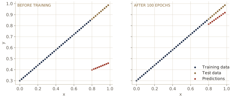
The predictions are nowhere near the test data. That is expected: the model has only random numbers to work with. Now we teach it.
Step 3: A loss function and an optimizer
Training needs two things: a way to measure how wrong the model is, and a way to make it less wrong.
The loss function measures the error
A loss function (also called a cost or criterion) compares the model’s predictions with the true values and returns a single number: lower is better, zero is perfect. For predicting numbers, a common choice is the mean absolute error (MAE): the average distance between each prediction \(\hat{y}_i\) and the true value \(y_i\),
\[\text{MAE} = \frac{1}{n}\sum_{i=1}^{n} \left\lvert\, y_i - \hat{y}_i \,\right\rvert\]In PyTorch it is called nn.L1Loss (the absolute difference is also known as the L1 distance). Let’s measure how far off the untrained model is:
loss_fn = nn.L1Loss()
loss_fn(y_preds, y_test)
tensor(0.4945)
On average, each test prediction is about 0.5 away from the truth — roughly the gap you can see in the plot.
The optimizer reduces the error
An optimizer updates the model’s parameters to lower the loss. The classic one is stochastic gradient descent (SGD), torch.optim.SGD. (“Stochastic”, meaning random, refers to its usual use on randomly chosen subsets of the data, which you will meet in module 03; here each step uses all 40 training points.) You tell it which parameters it may change and how big its steps should be:
optimizer = torch.optim.SGD(params=model_0.parameters(), lr=0.01)
lr is the learning rate: how large a step the optimizer takes each time. It is a hyperparameter — a setting that you choose, as opposed to a parameter, which the model learns. Too small a learning rate and training crawls; too large and the parameters jump past the best values and may never settle. Common starting values are 0.1, 0.01, and 0.001.
Which loss and optimizer to use depends on the problem. For now, these are enough: L1 loss (or mean squared error, nn.MSELoss) for predicting numbers; binary cross entropy for yes/no classification (next module); SGD or Adam (torch.optim.Adam) as the optimizer.
How learning works: gradients and gradient descent
Imagine plotting the loss against the value of a single weight. For each possible weight you would get a different loss, and the plot would form a valley. The best weight is at the bottom. We cannot see the whole valley, but at the point where we stand we can measure the slope.
That slope is the gradient, written \(\partial L / \partial w\): how much the loss \(L\) changes when the weight \(w\) is nudged a little. If the gradient is positive, increasing the weight increases the loss, so we should decrease the weight; if negative, the opposite. Either way, the rule is to step against the gradient:
\[w \leftarrow w - \text{lr} \cdot \frac{\partial L}{\partial w}\]and the same for the bias, and for every other parameter. Repeat the step many times and the parameters walk downhill to the bottom of the valley. That is gradient descent.
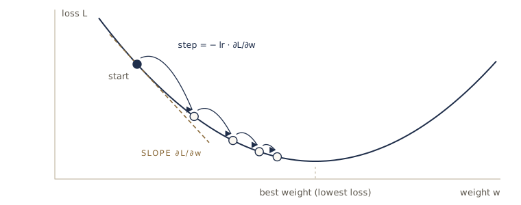
Where do the gradients come from? A model can have millions of parameters, and working out each slope by hand would be hopeless. PyTorch does it automatically, a feature called autograd. During the forward pass it records every operation applied to tensors marked requires_grad=True. When you call loss.backward(), it runs back through that record and applies the chain rule of calculus to compute the gradient of the loss with respect to every parameter. That backward sweep is called backpropagation. The gradient of each parameter is stored in its .grad attribute.
Let’s watch one step of learning. First, one forward pass and one backward pass:
y_pred = model_0(X_train)          # forward pass
loss = loss_fn(y_pred, y_train)    # how wrong?
loss.backward()                    # backpropagation: compute the gradients

print(f"Loss: {loss.item():.4f}")
print(f"Gradient of the weight: {model_0.weights.grad.item():.4f}")
print(f"Gradient of the bias:   {model_0.bias.grad.item():.4f}")
Loss: 0.3129
Gradient of the weight: -0.3900
Gradient of the bias:   -1.0000
Both gradients are negative: increasing the weight or the bias would reduce the loss (every prediction is currently too low). Now let the optimizer take its step:
w_before = model_0.weights.item()
optimizer.step()                   # w <- w - lr * grad
w_after = model_0.weights.item()

expected_change = -0.01 * model_0.weights.grad.item()   # -lr * grad
print(f"Weight before:   {w_before:.4f}")
print(f"Weight after:    {w_after:.4f}")
print(f"Change:          {w_after - w_before:.4f}")
print(f"-lr * gradient:  {expected_change:.4f}")
Weight before:   0.3367
Weight after:    0.3406
Change:          0.0039
-lr * gradient:  0.0039
The weight moved up by exactly the learning rate times the gradient, as the update rule says. Training is nothing more than this, repeated.
Note. You do not need to compute derivatives yourself in this course — autograd does it. What you need is the picture: the gradient says which way is uphill, and the optimizer steps the other way.
Before we train properly, put the model back to its starting values so that your numbers match the notes:
torch.manual_seed(42)
model_0 = LinearRegressionModel()
optimizer = torch.optim.SGD(params=model_0.parameters(), lr=0.01)
Step 4: The training loop
Five steps, in order
Training repeats the same five steps. One pass through all of the training data is called an epoch.
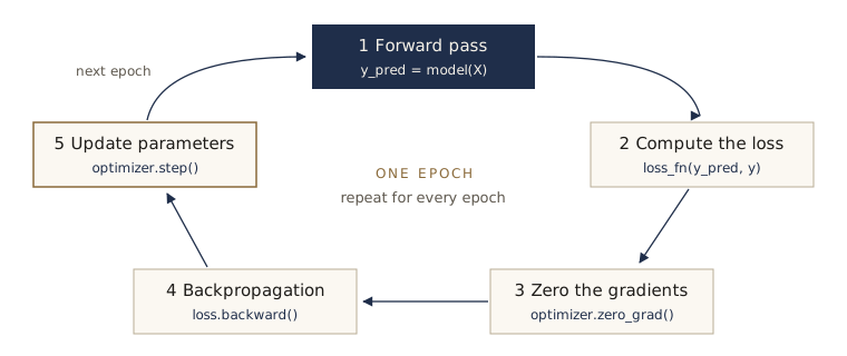
backward() computes new ones, and step() can only use gradients that exist.| Step | Code | What it does |
|---|---|---|
| 1. Forward pass | y_pred = model(X_train) |
The model makes predictions on the training data |
| 2. Compute the loss | loss = loss_fn(y_pred, y_train) |
Measure how wrong the predictions are |
| 3. Zero the gradients | optimizer.zero_grad() |
Clear the gradients left over from the last step |
| 4. Backpropagation | loss.backward() |
Compute the gradient of the loss for every parameter |
| 5. Optimizer step | optimizer.step() |
Nudge each parameter against its gradient |
Two details need explaining.
Why zero the gradients? PyTorch adds new gradients to whatever is already stored in .grad instead of replacing it. That is handy in some advanced cases, but in an ordinary loop it would mean each step uses the sum of all past gradients — steps would grow and grow. So we clear them once per loop, before calling backward(). (Our one-step experiment above did not need it only because the gradients started empty.)
model.train() and model.eval(). A model has two modes. model.train() puts it in training mode; model.eval() puts it in evaluation mode. Our straight-line model behaves the same in both, but some layers you will meet later (dropout, batch normalization) behave differently while training and while being tested. Setting the mode every time is a habit worth forming now.
The testing loop
After each epoch (or every few), we check the model on the test data. The testing loop is shorter — no learning happens:
| Step | Code | What it does |
|---|---|---|
| 1. Forward pass | test_pred = model(X_test) |
Predictions on data the model has not trained on |
| 2. Compute the loss | test_loss = loss_fn(test_pred, y_test) |
How wrong on unseen data? |
| 3. (Optional) Other metrics | e.g. accuracy | Anything else you want to monitor |
It runs in model.eval() mode and inside torch.inference_mode(), and it never calls zero_grad, backward, or step.
Training for real
Here is the whole thing. We train for 100 epochs, test every epoch, and record the losses every 10 epochs so we can plot them afterwards:
torch.manual_seed(42)
epochs = 100

# Lists to track progress
epoch_count = []
train_loss_values = []
test_loss_values = []

for epoch in range(epochs):
    ### Training
    model_0.train()                      # training mode

    y_pred = model_0(X_train)            # 1. forward pass
    loss = loss_fn(y_pred, y_train)      # 2. compute the loss
    optimizer.zero_grad()                # 3. zero the gradients
    loss.backward()                      # 4. backpropagation
    optimizer.step()                     # 5. update the parameters

    ### Testing
    model_0.eval()                       # evaluation mode
    with torch.inference_mode():
        test_pred = model_0(X_test)              # 1. forward pass
        test_loss = loss_fn(test_pred, y_test)   # 2. test loss

    if epoch % 10 == 0:
        epoch_count.append(epoch)
        train_loss_values.append(loss.item())
        test_loss_values.append(test_loss.item())
        print(f"Epoch: {epoch:3d} | Train loss: {loss.item():.4f} "
              f"| Test loss: {test_loss.item():.4f}")
Epoch:   0 | Train loss: 0.3129 | Test loss: 0.4811
Epoch:  10 | Train loss: 0.1977 | Test loss: 0.3464
Epoch:  20 | Train loss: 0.0891 | Test loss: 0.2173
Epoch:  30 | Train loss: 0.0531 | Test loss: 0.1446
Epoch:  40 | Train loss: 0.0454 | Test loss: 0.1136
Epoch:  50 | Train loss: 0.0417 | Test loss: 0.0992
Epoch:  60 | Train loss: 0.0382 | Test loss: 0.0889
Epoch:  70 | Train loss: 0.0348 | Test loss: 0.0806
Epoch:  80 | Train loss: 0.0313 | Test loss: 0.0723
Epoch:  90 | Train loss: 0.0279 | Test loss: 0.0647
Both losses fall steadily. The test loss starts higher than the training loss (the test points lie beyond the training range, where a wrong slope hurts most) and then drops faster. Now compare the learned parameters with the true ones:
print("Learned values:")
for name, value in model_0.state_dict().items():
    print(f"  {name}: {value}")
print(f"True values:\n  weights: {weight}, bias: {bias}")
Learned values:
  weights: tensor([0.5784])
  bias: tensor([0.3513])
True values:
  weights: 0.7, bias: 0.3
Starting from random numbers, the bias has already reached the neighborhood of \(b = 0.3\) and the weight has covered about two-thirds of the distance to \(w = 0.7\) — without the model ever being told either value. More epochs would bring it closer still. That is the core idea of machine learning in miniature.
Loss curves
A loss curve plots the loss against the epoch. It is the first thing to look at after any training run.
plt.plot(epoch_count, train_loss_values, label="Train loss")
plt.plot(epoch_count, test_loss_values, label="Test loss")
plt.ylabel("Loss")
plt.xlabel("Epoch")
plt.legend()
plt.show()
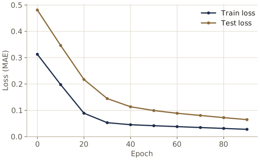
Both curves falling is what you want. Later you will learn to read the unhealthy shapes: a training loss that stays high (the model cannot fit even the data it trains on — underfitting), and a test loss that rises while the training loss keeps falling (the model is memorizing the training set — overfitting). Module 04 treats both in detail.
Step 5: Making predictions with a trained model
When you use a model for predictions, remember three things:
- Put the model in evaluation mode:
model.eval(). - Make the predictions inside
with torch.inference_mode():. - Keep the model and the data on the same device (both on the CPU, or both on the GPU).
model_0.eval()
with torch.inference_mode():
    y_preds = model_0(X_test)

y_preds[:5]
tensor([[0.8141],
        [0.8256],
        [0.8372],
        [0.8488],
        [0.8603]])
plot_predictions(predictions=y_preds)
This is the right panel of the figure in step 2: the predictions now sit much closer to the test points, though still a little below them — the learned weight (0.58) is smaller than the true 0.7, so the line is not yet steep enough. Training for more epochs would close the gap.
Step 6: Saving and loading a model
Training takes time, so you save the result. PyTorch has three functions for this:
| Function | What it does |
|---|---|
torch.save(obj, f) |
Write a Python object (such as a state dict) to a file |
torch.load(f) |
Read it back |
model.load_state_dict(state_dict) |
Copy saved parameter values into a model |
The recommended approach is to save only the model’s state_dict() — the learned numbers — rather than the whole model object. It is smaller and less fragile: the file does not depend on the exact folder layout of your code.
Saving
from pathlib import Path

# 1. Make a folder for models
MODEL_PATH = Path("models")
MODEL_PATH.mkdir(parents=True, exist_ok=True)

# 2. Choose a file name (PyTorch files end in .pt or .pth)
MODEL_NAME = "01_pytorch_workflow_model_0.pth"
MODEL_SAVE_PATH = MODEL_PATH / MODEL_NAME

# 3. Save the state dict
print(f"Saving model to: {MODEL_SAVE_PATH}")
torch.save(obj=model_0.state_dict(), f=MODEL_SAVE_PATH)
Saving model to: models/01_pytorch_workflow_model_0.pth
Path from Python’s pathlib library builds file paths that work on Windows, macOS, and Linux alike; the / operator joins a folder and a file name.
Loading
A state dict holds numbers only, so to load it you first need a model with the same structure. Create a fresh instance (with new random parameters), then copy the saved values in:
loaded_model_0 = LinearRegressionModel()
loaded_model_0.load_state_dict(torch.load(f=MODEL_SAVE_PATH))
<All keys matched successfully>
<All keys matched successfully> means every saved parameter found its place in the new model. To be sure nothing was lost, compare the loaded model’s predictions with the original’s:
loaded_model_0.eval()
with torch.inference_mode():
    loaded_model_preds = loaded_model_0(X_test)

torch.equal(y_preds, loaded_model_preds)
True
Identical predictions: the loaded model is the trained model.
Note. In Colab, files you save disappear when the runtime shuts down. Download anything you want to keep (Files panel on the left → right-click → Download), or save to your Google Drive.
Putting it all together
Now we run the whole workflow again in one place, with two upgrades you will use from here on: a built-in layer instead of hand-made parameters, and code that runs on a GPU when one is available.
Setup and device-agnostic code
import torch
from torch import nn
import matplotlib.pyplot as plt

device = "cuda" if torch.cuda.is_available() else "cpu"
print(f"Using device: {device}")
Using device: cpu
On a Colab GPU runtime this prints cuda; the notes were run on a CPU.
Data
weight = 0.7
bias = 0.3

X = torch.arange(0, 1, 0.02).unsqueeze(dim=1)
y = weight * X + bias

train_split = int(0.8 * len(X))
X_train, y_train = X[:train_split], y[:train_split]
X_test, y_test = X[train_split:], y[train_split:]

len(X_train), len(X_test)
(40, 10)
A model built from nn.Linear
Writing nn.Parameters by hand was useful for seeing what a model contains, but in practice you use ready-made layers. nn.Linear computes exactly \(y = x A^{\top} + b\) — the linear layer from module 00 — and creates and initializes its weight and bias for you. With one input feature and one output feature, it is our straight line:
class LinearRegressionModelV2(nn.Module):
    def __init__(self):
        super().__init__()
        self.linear_layer = nn.Linear(in_features=1, out_features=1)

    def forward(self, x: torch.Tensor) -> torch.Tensor:
        return self.linear_layer(x)

torch.manual_seed(42)
model_1 = LinearRegressionModelV2()
print(model_1)
for name, value in model_1.state_dict().items():
    print(f"{name}: {value}")
LinearRegressionModelV2(
  (linear_layer): Linear(in_features=1, out_features=1, bias=True)
)
linear_layer.weight: tensor([[0.7645]])
linear_layer.bias: tensor([0.8300])
The state dict now names the parameters linear_layer.weight and linear_layer.bias. Printing the model shows its layers — handy once models have dozens of them.
Models are created on the CPU. Move the model to the target device, and check where its parameters live:
model_1.to(device)
next(model_1.parameters()).device
device(type='cpu')
Training
The loss and optimizer are the same as before. Note that the optimizer is given model_1.parameters() — an optimizer can only update the parameters you hand it. We also move the data to the device, because a model on the GPU cannot work with data on the CPU:
loss_fn = nn.L1Loss()
optimizer = torch.optim.SGD(params=model_1.parameters(), lr=0.01)

# Put the data on the same device as the model
X_train, y_train = X_train.to(device), y_train.to(device)
X_test, y_test = X_test.to(device), y_test.to(device)

torch.manual_seed(42)
epochs = 1000

for epoch in range(epochs):
    ### Training
    model_1.train()
    y_pred = model_1(X_train)
    loss = loss_fn(y_pred, y_train)
    optimizer.zero_grad()
    loss.backward()
    optimizer.step()

    ### Testing
    model_1.eval()
    with torch.inference_mode():
        test_pred = model_1(X_test)
        test_loss = loss_fn(test_pred, y_test)

    if epoch % 100 == 0:
        print(f"Epoch: {epoch:3d} | Train loss: {loss.item():.4f} "
              f"| Test loss: {test_loss.item():.4f}")
Epoch:   0 | Train loss: 0.5552 | Test loss: 0.5740
Epoch: 100 | Train loss: 0.0062 | Test loss: 0.0141
Epoch: 200 | Train loss: 0.0013 | Test loss: 0.0138
Epoch: 300 | Train loss: 0.0013 | Test loss: 0.0138
Epoch: 400 | Train loss: 0.0013 | Test loss: 0.0138
Epoch: 500 | Train loss: 0.0013 | Test loss: 0.0138
Epoch: 600 | Train loss: 0.0013 | Test loss: 0.0138
Epoch: 700 | Train loss: 0.0013 | Test loss: 0.0138
Epoch: 800 | Train loss: 0.0013 | Test loss: 0.0138
Epoch: 900 | Train loss: 0.0013 | Test loss: 0.0138
By epoch 200 the loss is close to zero and stops changing. It never reaches exactly zero: with a fixed learning rate, SGD keeps stepping back and forth across the bottom of the valley, so the parameters hover near the best values instead of landing on them. Check the parameters:
print("Learned values:")
for name, value in model_1.state_dict().items():
    print(f"  {name}: {value}")
print(f"True values:\n  weights: {weight}, bias: {bias}")
Learned values:
  linear_layer.weight: tensor([[0.6968]])
  linear_layer.bias: tensor([0.3025])
True values:
  weights: 0.7, bias: 0.3
Very close to 0.7 and 0.3.
Predictions
model_1.eval()
with torch.inference_mode():
    y_preds = model_1(X_test)

# Matplotlib works with NumPy, which lives on the CPU
plot_predictions(train_data=X_train.cpu(), train_labels=y_train.cpu(),
                 test_data=X_test.cpu(), test_labels=y_test.cpu(),
                 predictions=y_preds.cpu())
If you forget .cpu() on a GPU runtime, matplotlib fails with can't convert cuda:0 device type tensor to numpy — the wrong device error from module 00.
Saving and loading
MODEL_NAME = "01_pytorch_workflow_model_1.pth"
MODEL_SAVE_PATH = MODEL_PATH / MODEL_NAME

torch.save(obj=model_1.state_dict(), f=MODEL_SAVE_PATH)

loaded_model_1 = LinearRegressionModelV2()
loaded_model_1.load_state_dict(torch.load(MODEL_SAVE_PATH))
loaded_model_1.to(device)

loaded_model_1.eval()
with torch.inference_mode():
    loaded_model_1_preds = loaded_model_1(X_test)

torch.equal(y_preds, loaded_model_1_preds)
True
The reloaded model makes the same predictions. That is the complete workflow: data, model, loss and optimizer, training loop, evaluation, and saving.
Note. If you save on a GPU and load on a CPU-only machine, pass
map_location="cpu"totorch.load. Loading the state dict into a model you have already moved to a device also works.
Summary
| Task | Code |
|---|---|
| Split data | X_train, X_test = X[:n], X[n:] |
| Define a model | subclass nn.Module; create parameters or layers in __init__; compute in forward |
| Learnable tensor | nn.Parameter(torch.randn(1)), or a layer such as nn.Linear(in_features, out_features) |
| Inspect a model | model.parameters(), model.state_dict() |
| Loss and optimizer | nn.L1Loss(), torch.optim.SGD(model.parameters(), lr=0.01) |
| One training step | model.train(); forward, loss, optimizer.zero_grad(), loss.backward(), optimizer.step() |
| Testing / predictions | model.eval() and with torch.inference_mode(): |
| Save and load | torch.save(model.state_dict(), path); model.load_state_dict(torch.load(path)) |
| Device | device = "cuda" if torch.cuda.is_available() else "cpu"; model.to(device), X.to(device) |
Three ideas to carry forward: a model is a function with adjustable numbers; the loss says how wrong it is and the gradient says which way to adjust; and the five-line training loop — forward, loss, zero grad, backward, step — is the same for every model in this course.
Exercises
Start a fresh Colab notebook and write the code yourself; resist copying from above.
- Create a straight-line dataset with
weight = 0.3andbias = 0.9, at least 100 points, and split it 80/20 into training and test sets. Plot it. - Build a model by subclassing
nn.Module, either with twonn.Parameters or withnn.Linear. Print itsstate_dict(). - Create an
nn.L1Lossloss and an SGD optimizer withlr=0.01. Train for 300 epochs, and print the training and test loss every 20 epochs. - Make predictions on the test data with the trained model and plot them against the true test data. How close are the learned weight and bias to 0.3 and 0.9?
- Save the model’s
state_dict(), load it into a new instance of the same class, and confirm that the two models make identical predictions. - Delete
optimizer.zero_grad()from your loop and train again from the same seed. Plot the loss curve. What changes, and why? - Train three models with learning rates 0.1, 0.01, and 0.001 for 100 epochs each. Plot the three training loss curves on one figure and describe the difference in words.
- In your own words. Pick a quantity in your engineering field that is roughly a straight-line function of another (for example, strain against stress in the elastic range). Describe what
X,y, the weight, and the bias would mean, and which part of the data you would hold back as a test set.
Going further
- The PyTorch tutorial Build the neural network covers
nn.Modulefrom a different angle. - A gentle introduction to
torch.autogradexplains gradients and backpropagation in more depth. - Saving and loading models — the official guide, including checkpoints for resuming training.
- The documentation for
torch.optimlists the available optimizers and their settings.
These notes follow the path of Daniel Bourke's Learn PyTorch for Deep Learning (MIT license), rewritten for engineering students meeting Python and machine learning for the first time.