EAS 510 · Module 02 · Week 3
Neural Network Classification
From predicting numbers to predicting categories — logits, sigmoid and softmax, accuracy, and why non-linearity matters.
Companion reading: Learn PyTorch for Deep Learning, chapter 02
By the end of this module you can
- Tell binary, multi-class, and multi-label classification apart, and choose the output layer, activation, and loss for each.
- Turn a model’s raw outputs (logits) into probabilities with sigmoid or softmax, and into class labels.
- Explain why
BCEWithLogitsLossis preferred overBCELoss, and train a binary classifier with it. - Plot a decision boundary and use it to diagnose a model that cannot fit its data.
- Explain why stacking linear layers still gives a straight line, and fix it with a non-linear activation such as ReLU.
- Improve a model by changing one thing at a time, and sanity-check it on a problem it should be able to solve.
- Build and evaluate a multi-class classifier with
CrossEntropyLoss, and report accuracy, precision, recall, F1, and a confusion matrix.
Contents
- What classification is
- Step 1: Making classification data
- Step 2: Building a model
- From logits to labels
- Step 3: Training the model
- Step 4: Diagnosing the model with a decision boundary
- Step 5: Improving a model
- Step 6: The missing piece — non-linearity
- Replicating the activation functions
- Multi-class classification
- More ways to measure a classifier
- Summary
- Exercises
- Going further
In module 01 a model learned to predict a number — a point on a straight line. Many engineering questions have a different kind of answer: is this weld good or defective? which of four defect types is on this steel sheet? Predicting a category is called classification, and it is the subject of this module.
The workflow does not change: data, model, loss and optimizer, training loop, evaluation. What changes is the end of the model and the way we measure error. Along the way we will meet the most important idea in this module — non-linearity — by building a model that fails, working out why, and fixing it.
What classification is
There are three kinds of classification problem:
| Kind | What the model answers | Engineering example | Everyday example |
|---|---|---|---|
| Binary | One of two classes | Is this weld good or defective? | Is this email spam? |
| Multi-class | One of more than two classes | Is this surface defect a scratch, pit, crack, or inclusion? | Is this photo pizza, steak, or sushi? |
| Multi-label | Any number of labels at once | Which of corrosion, cracking, spalling appear in this bridge photo? | Which topic tags fit this article? |
In binary and multi-class problems each sample belongs to exactly one class. In multi-label problems a sample can have several labels, or none. This module covers binary and multi-class; multi-label uses the same tools with a small twist (a sigmoid for every label).
The shape of a classification network
Whatever the problem, a classification network has the same outline. Only a few pieces differ between binary and multi-class:
| Part of the network | Binary classification | Multi-class classification |
|---|---|---|
Input layer (in_features) |
Number of features (e.g. 2 coordinates) | Same |
| Hidden layers | Problem-specific; at least one | Same |
| Neurons per hidden layer | Problem-specific; commonly 10 to 512 | Same |
Output layer (out_features) |
1 | One per class |
| Hidden-layer activation | Usually ReLU | Same |
| Output activation | Sigmoid | Softmax |
| Loss function | Binary cross entropy (nn.BCEWithLogitsLoss) |
Cross entropy (nn.CrossEntropyLoss) |
| Optimizer | SGD or Adam | Same |
Don’t worry if some entries are new; we will meet each of them in this module and come back to this table at the end.
Step 1: Making classification data
Two circles
We use a toy dataset from scikit-learn, a popular Python library for classical machine learning. make_circles draws points on two circles, one inside the other. Each point has two features (its \(x_1\) and \(x_2\) coordinates) and a label: 0 for the outer circle, 1 for the inner one.
import torch
from torch import nn
import matplotlib.pyplot as plt
from sklearn.datasets import make_circles

n_samples = 1000
X, y = make_circles(n_samples, noise=0.03, random_state=42)

print(f"First 5 samples of X:\n{X[:5]}")
print(f"First 5 labels of y: {y[:5]}")
First 5 samples of X:
[[ 0.75424625  0.23148074]
 [-0.75615888  0.15325888]
 [-0.81539193  0.17328203]
 [-0.39373073  0.69288277]
 [ 0.44220765 -0.89672343]]
First 5 labels of y: [1 1 1 1 0]
noise=0.03 jitters the points slightly so the circles are not perfect, and random_state=42 is scikit-learn’s version of a random seed. A plot shows the problem at once:
plt.scatter(x=X[:, 0], y=X[:, 1], c=y, cmap=plt.cm.RdYlBu, s=10)
plt.show()
The task is to learn, from the coordinates alone, which circle a point belongs to. No straight line can separate the two classes — remember that; it is the crux of this module. A toy problem like this is small enough to train in seconds, yet it has all the parts of a real one. Think of it as sorting parts into “pass” and “fail” from two measurements, where the good parts cluster near the nominal values and the faulty ones lie in a ring around them.
Input and output shapes
Checking shapes before building anything saves a lot of confusion:
print(f"X shape: {X.shape},  y shape: {y.shape}")
print(f"One sample: X = {X[0]}, y = {y[0]}")
print(f"Features per sample: {X[0].shape},  label: a single number {y[0].shape}")
X shape: (1000, 2),  y shape: (1000,)
One sample: X = [0.75424625 0.23148074], y = 1
Features per sample: (2,),  label: a single number ()
1,000 samples, each with two features in and one label out. So the model will take 2 numbers in and give 1 number out.
Tensors and a train/test split
The data comes from scikit-learn as NumPy arrays of 64-bit floats. We convert them to PyTorch’s default float32 (recall the warning in module 00), then split them. Unlike the line in module 01, these samples have no natural order to respect, so rather than cutting at a position we use scikit-learn’s train_test_split, which shuffles and splits in one call:
from sklearn.model_selection import train_test_split

X = torch.from_numpy(X).type(torch.float32)
y = torch.from_numpy(y).type(torch.float32)

X_train, X_test, y_train, y_test = train_test_split(
    X, y, test_size=0.2, random_state=42)   # 20% test, 80% train

len(X_train), len(X_test), len(y_train), len(y_test)
(800, 200, 800, 200)
800 samples to learn from, 200 held back for testing.
Step 2: Building a model
Device-agnostic setup
As in module 01, write the code so it uses a GPU when there is one:
device = "cuda" if torch.cuda.is_available() else "cpu"
device
'cpu'
A first model
Our first model has two nn.Linear layers. The first takes the 2 features and produces 5 numbers; the second takes those 5 and produces 1 number:
class CircleModelV0(nn.Module):
    def __init__(self):
        super().__init__()
        self.layer_1 = nn.Linear(in_features=2, out_features=5)   # 2 features in
        self.layer_2 = nn.Linear(in_features=5, out_features=1)   # 1 number out

    def forward(self, x):
        return self.layer_2(self.layer_1(x))   # x -> layer_1 -> layer_2

torch.manual_seed(42)
model_0 = CircleModelV0().to(device)
model_0
CircleModelV0(
  (layer_1): Linear(in_features=2, out_features=5, bias=True)
  (layer_2): Linear(in_features=5, out_features=1, bias=True)
)
The 5 numbers in the middle form a hidden layer: hidden because you never see them in the input or the output. The number of hidden units (here 5) is a hyperparameter. More hidden units give the model more room to find patterns, up to a point. The one rule you must follow is the shape rule from module 00: each layer’s in_features must equal the previous layer’s out_features.
For a model that just passes data through a list of layers in order, PyTorch has a shortcut, nn.Sequential. This builds the same network without writing a class:
torch.manual_seed(42)
model_0_seq = nn.Sequential(
    nn.Linear(in_features=2, out_features=5),
    nn.Linear(in_features=5, out_features=1)
).to(device)
model_0_seq
Sequential(
  (0): Linear(in_features=2, out_features=5, bias=True)
  (1): Linear(in_features=5, out_features=1, bias=True)
)
nn.Sequential is convenient, but it always runs its layers one after the other. Subclassing nn.Module lets you write any computation you like in forward, so we will mostly use it and put nn.Sequential blocks inside it.
Predictions from the untrained model
with torch.inference_mode():
    untrained_preds = model_0(X_test.to(device))

print(f"Shape of predictions: {untrained_preds.shape}")
print(f"Shape of test labels: {y_test.shape}")
print(f"First 5 predictions:\n{untrained_preds[:5]}")
print(f"First 5 labels: {y_test[:5]}")
Shape of predictions: torch.Size([200, 1])
Shape of test labels: torch.Size([200])
First 5 predictions:
tensor([[-0.1269],
        [-0.0967],
        [-0.1908],
        [-0.1089],
        [-0.1667]])
First 5 labels: tensor([1., 0., 1., 0., 1.])
Two things to notice. The predictions have shape [200, 1] while the labels have shape [200] — we will remove the extra dimension with squeeze(). And the predictions are not 0s and 1s; they are arbitrary numbers. Turning them into labels is the next topic.
From logits to labels
Logits, probabilities, and labels
The raw numbers that come out of the last layer are called logits. A logit can be any number, positive or negative, and on its own it does not mean much. To get something useful we pass it through an activation function that squeezes it into a probability.
For binary classification that function is the sigmoid:
\[\sigma(z) = \frac{1}{1 + e^{-z}}\]It maps any number \(z\) to a number between 0 and 1: large positive logits give probabilities near 1, large negative logits give probabilities near 0, and a logit of 0 gives exactly 0.5. We read the result as the probability that the sample belongs to class 1. Finally, a threshold turns the probability into a label: above 0.5 means class 1, below means class 0. Rounding does exactly that.
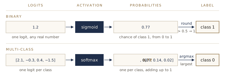
Let’s apply this to the untrained model’s first five outputs:
with torch.inference_mode():
    y_logits = model_0(X_test.to(device))[:5]
y_logits
tensor([[-0.1269],
        [-0.0967],
        [-0.1908],
        [-0.1089],
        [-0.1667]])
y_pred_probs = torch.sigmoid(y_logits)
y_pred_probs
tensor([[0.4683],
        [0.4758],
        [0.4524],
        [0.4728],
        [0.4584]])
y_preds = torch.round(y_pred_probs)
print(y_preds.squeeze())
print(y_test[:5])
tensor([0., 0., 0., 0., 0.])
tensor([1., 0., 1., 0., 1.])
Logits → sigmoid → round → labels. All in one line, for the whole test set, it reads torch.round(torch.sigmoid(model(X))). The untrained model’s labels match the truth only by chance.
Loss function: binary cross entropy
For classification we need a loss that rewards confident correct answers and punishes confident wrong ones. That loss is binary cross entropy (BCE). For predicted probabilities \(p_i\) and true labels \(y_i \in \{0, 1\}\),
\[\text{BCE} = -\frac{1}{n}\sum_{i=1}^{n}\Big[\,y_i \log p_i + (1 - y_i)\log(1 - p_i)\,\Big]\]Only one of the two terms is active for each sample. If the label is 1, the loss is \(-\log p_i\): close to 0 when \(p_i\) is near 1, and very large when the model confidently says 0. If the label is 0, it is \(-\log(1 - p_i)\), the mirror image.
PyTorch offers two versions:
nn.BCELossexpects probabilities, so you apply the sigmoid yourself first.nn.BCEWithLogitsLossexpects logits and applies the sigmoid inside.
They compute the same thing:
y_true = torch.tensor([1., 0., 1.])
logits = torch.tensor([2.0, -1.0, -0.5])

print(nn.BCELoss()(torch.sigmoid(logits), y_true))
print(nn.BCEWithLogitsLoss()(logits, y_true))
tensor(0.4714)
tensor(0.4714)
Use nn.BCEWithLogitsLoss. Combining the two steps lets PyTorch use a formula that is numerically stable: when a logit is very large or very negative, a separate sigmoid can round to exactly 0 or 1, and then \(\log 0\) turns the loss into infinity. The combined version never takes that logarithm directly.
Watch out. With
BCEWithLogitsLoss, feed the model’s raw logits to the loss — nottorch.sigmoid(logits). Applying the sigmoid twice still runs without an error, but the model learns badly.
loss_fn = nn.BCEWithLogitsLoss()
optimizer = torch.optim.SGD(params=model_0.parameters(), lr=0.1)
An evaluation metric: accuracy
The loss is what the optimizer minimizes, but it is not easy for a person to interpret. Alongside it we track an evaluation metric, a number that says how well the model does in human terms. The simplest is accuracy: out of all predictions, what percentage were right?
def accuracy_fn(y_true, y_pred):
    """Percentage of predictions that match the true labels."""
    correct = torch.eq(y_true, y_pred).sum().item()
    return (correct / len(y_pred)) * 100
torch.eq compares element by element and returns True where the two tensors agree; .sum() counts the Trues.
Step 3: Training the model
The loop is the one from module 01, with two additions: we turn logits into labels to compute accuracy, and we squeeze() the model output so its shape [800, 1] matches the labels’ shape [800].
torch.manual_seed(42)
epochs = 100

X_train, y_train = X_train.to(device), y_train.to(device)
X_test, y_test = X_test.to(device), y_test.to(device)

for epoch in range(epochs):
    ### Training
    model_0.train()
    y_logits = model_0(X_train).squeeze()             # forward pass -> logits
    y_pred = torch.round(torch.sigmoid(y_logits))     # logits -> labels
    loss = loss_fn(y_logits, y_train)                 # the loss takes logits
    acc = accuracy_fn(y_true=y_train, y_pred=y_pred)
    optimizer.zero_grad()
    loss.backward()
    optimizer.step()

    ### Testing
    model_0.eval()
    with torch.inference_mode():
        test_logits = model_0(X_test).squeeze()
        test_pred = torch.round(torch.sigmoid(test_logits))
        test_loss = loss_fn(test_logits, y_test)
        test_acc = accuracy_fn(y_true=y_test, y_pred=test_pred)

    if epoch % 10 == 0:
        print(f"Epoch: {epoch:3d} | Loss: {loss:.5f}, Acc: {acc:.2f}% "
              f"| Test loss: {test_loss:.5f}, Test acc: {test_acc:.2f}%")
Epoch:   0 | Loss: 0.69569, Acc: 50.00% | Test loss: 0.69721, Test acc: 50.00%
Epoch:  10 | Loss: 0.69403, Acc: 50.00% | Test loss: 0.69615, Test acc: 50.00%
Epoch:  20 | Loss: 0.69343, Acc: 46.00% | Test loss: 0.69585, Test acc: 48.50%
Epoch:  30 | Loss: 0.69321, Acc: 49.00% | Test loss: 0.69577, Test acc: 47.50%
Epoch:  40 | Loss: 0.69312, Acc: 49.50% | Test loss: 0.69573, Test acc: 46.50%
Epoch:  50 | Loss: 0.69308, Acc: 50.38% | Test loss: 0.69569, Test acc: 46.50%
Epoch:  60 | Loss: 0.69306, Acc: 50.50% | Test loss: 0.69564, Test acc: 46.50%
Epoch:  70 | Loss: 0.69305, Acc: 50.50% | Test loss: 0.69559, Test acc: 46.50%
Epoch:  80 | Loss: 0.69304, Acc: 50.75% | Test loss: 0.69553, Test acc: 46.50%
Epoch:  90 | Loss: 0.69303, Acc: 50.38% | Test loss: 0.69547, Test acc: 46.50%
Something is wrong. The loss barely moves, and the accuracy hovers around 50% — exactly what you would get by flipping a coin. With two balanced classes (500 samples each), the model has learned nothing.
Step 4: Diagnosing the model with a decision boundary
When a number says “bad”, a picture usually says why. A decision boundary shows which class the model predicts at every point of the input space. We make a fine grid of points covering the data, ask the model for a prediction at each one, and color the plane by the answer. Here is a small helper; read the comments rather than memorizing it:
def plot_decision_boundary(model, X, y, n=101):
    """Color the plane by the model's predicted class and overlay the data."""
    X, y = X.cpu(), y.cpu()
    model_device = next(model.parameters()).device

    # 1. A grid of n x n points that covers the data, with a small margin
    x1 = torch.linspace(X[:, 0].min() - 0.1, X[:, 0].max() + 0.1, n)
    x2 = torch.linspace(X[:, 1].min() - 0.1, X[:, 1].max() + 0.1, n)
    xx1, xx2 = torch.meshgrid(x1, x2, indexing="xy")
    grid = torch.stack([xx1.ravel(), xx2.ravel()], dim=1)   # shape [n*n, 2]

    # 2. Predict a class for every grid point
    model.eval()
    with torch.inference_mode():
        logits = model(grid.to(model_device)).cpu()
    if logits.shape[1] == 1:                                  # binary
        preds = torch.round(torch.sigmoid(logits)).squeeze()
    else:                                                     # multi-class
        preds = torch.softmax(logits, dim=1).argmax(dim=1)

    # 3. Color the plane by prediction, then draw the data on top
    plt.contourf(xx1, xx2, preds.reshape(n, n), cmap=plt.cm.RdYlBu, alpha=0.6)
    plt.scatter(X[:, 0], X[:, 1], c=y, s=10, cmap=plt.cm.RdYlBu,
                edgecolors="k", linewidths=0.3)
Use it on the training and test data side by side:
plt.figure(figsize=(12, 5))
plt.subplot(1, 2, 1)
plt.title("Train")
plot_decision_boundary(model_0, X_train, y_train)
plt.subplot(1, 2, 2)
plt.title("Test")
plot_decision_boundary(model_0, X_test, y_test)
plt.show()
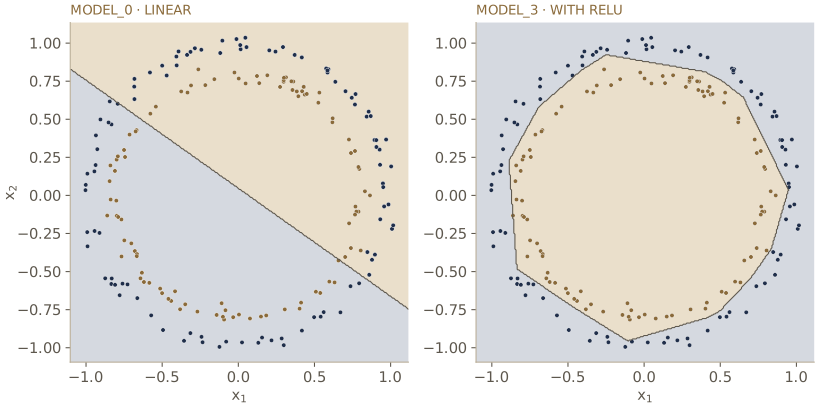
model_0 can only draw a straight line, so it cuts both circles in half — hence 50% accuracy. Right: model_3, the non-linear model we build in the section on non-linearity, bends its boundary around the inner circle.The left panel explains everything: the model has drawn a straight line through the middle of the circles. However you place a straight line, it cannot separate a ring from its center. The model is underfitting — it cannot capture the pattern in the data, even on the data it trains on.
Step 5: Improving a model
Things you can change
From the model’s side, there are several levers you can pull:
| Change | Why it might help |
|---|---|
| Add more layers | Each layer is another chance to learn a pattern; the model becomes deeper |
| Add more hidden units | More numbers per layer; the model becomes wider |
| Train for longer (more epochs) | The model gets more chances to learn |
| Change the activation functions | Non-linear activations let the model draw curves (see below) |
| Change the learning rate | Too small crawls; too large overshoots |
| Change the loss function | A different problem may need a different loss |
| Use transfer learning | Start from a model that already learned something useful (module 06) |
Most of these are hyperparameters (module 01): choices you make, not numbers the model learns. Machine learning practice is largely a matter of trying them in a disciplined way.
Habit. Change one thing at a time, and write down what you changed and what happened. If you change three things and the model improves, you will not know which one mattered. This is the idea behind experiment tracking in module 07.
A bigger model
Let’s pull three levers together — more hidden units (5 → 10), one more layer (2 → 3), and more epochs (100 → 1,000). (We just said to change one thing at a time; we break the rule here to save space, and the section on non-linearity explains why none of these changes could have helped on its own.)
class CircleModelV1(nn.Module):
    def __init__(self):
        super().__init__()
        self.layer_1 = nn.Linear(in_features=2, out_features=10)
        self.layer_2 = nn.Linear(in_features=10, out_features=10)   # extra layer
        self.layer_3 = nn.Linear(in_features=10, out_features=1)

    def forward(self, x):
        return self.layer_3(self.layer_2(self.layer_1(x)))

torch.manual_seed(42)
model_1 = CircleModelV1().to(device)

loss_fn = nn.BCEWithLogitsLoss()
optimizer = torch.optim.SGD(params=model_1.parameters(), lr=0.1)

torch.manual_seed(42)
epochs = 1000

for epoch in range(epochs):
    model_1.train()
    y_logits = model_1(X_train).squeeze()
    y_pred = torch.round(torch.sigmoid(y_logits))
    loss = loss_fn(y_logits, y_train)
    acc = accuracy_fn(y_true=y_train, y_pred=y_pred)
    optimizer.zero_grad()
    loss.backward()
    optimizer.step()

    model_1.eval()
    with torch.inference_mode():
        test_logits = model_1(X_test).squeeze()
        test_pred = torch.round(torch.sigmoid(test_logits))
        test_loss = loss_fn(test_logits, y_test)
        test_acc = accuracy_fn(y_true=y_test, y_pred=test_pred)

    if epoch % 100 == 0:
        print(f"Epoch: {epoch:4d} | Loss: {loss:.5f}, Acc: {acc:.2f}% "
              f"| Test loss: {test_loss:.5f}, Test acc: {test_acc:.2f}%")
Epoch:    0 | Loss: 0.69396, Acc: 50.88% | Test loss: 0.69261, Test acc: 51.00%
Epoch:  100 | Loss: 0.69305, Acc: 50.38% | Test loss: 0.69379, Test acc: 48.00%
Epoch:  200 | Loss: 0.69299, Acc: 51.12% | Test loss: 0.69437, Test acc: 46.00%
Epoch:  300 | Loss: 0.69298, Acc: 51.62% | Test loss: 0.69458, Test acc: 45.00%
Epoch:  400 | Loss: 0.69298, Acc: 51.12% | Test loss: 0.69465, Test acc: 46.00%
Epoch:  500 | Loss: 0.69298, Acc: 51.00% | Test loss: 0.69467, Test acc: 46.00%
Epoch:  600 | Loss: 0.69298, Acc: 51.00% | Test loss: 0.69468, Test acc: 46.00%
Epoch:  700 | Loss: 0.69298, Acc: 51.00% | Test loss: 0.69468, Test acc: 46.00%
Epoch:  800 | Loss: 0.69298, Acc: 51.00% | Test loss: 0.69468, Test acc: 46.00%
Epoch:  900 | Loss: 0.69298, Acc: 51.00% | Test loss: 0.69468, Test acc: 46.00%
Still a coin flip. A bigger model trained for longer did not help at all.
A sanity check: can it fit a straight line?
When a model fails, a useful trick is to test it on a problem it should be able to solve. If it fails that too, the bug is in the model or the training code; if it succeeds, the problem lies in the match between model and data. So let’s hand the same kind of model the straight-line data from module 01.
weight, bias = 0.7, 0.3
X_regression = torch.arange(0, 1, 0.01).unsqueeze(dim=1)
y_regression = weight * X_regression + bias

train_split = int(0.8 * len(X_regression))
X_train_regression = X_regression[:train_split]
y_train_regression = y_regression[:train_split]
X_test_regression = X_regression[train_split:]
y_test_regression = y_regression[train_split:]

len(X_train_regression), len(X_test_regression)
(80, 20)
The same three linear layers, now built with nn.Sequential, with 1 input feature instead of 2. Because this is a regression problem again, we switch back to L1 loss:
torch.manual_seed(42)
model_2 = nn.Sequential(
    nn.Linear(in_features=1, out_features=10),
    nn.Linear(in_features=10, out_features=10),
    nn.Linear(in_features=10, out_features=1)
).to(device)

loss_fn = nn.L1Loss()
optimizer = torch.optim.SGD(params=model_2.parameters(), lr=0.01)

X_train_regression = X_train_regression.to(device)
y_train_regression = y_train_regression.to(device)
X_test_regression = X_test_regression.to(device)
y_test_regression = y_test_regression.to(device)

torch.manual_seed(42)
epochs = 1000
for epoch in range(epochs):
    model_2.train()
    y_pred = model_2(X_train_regression)
    loss = loss_fn(y_pred, y_train_regression)
    optimizer.zero_grad()
    loss.backward()
    optimizer.step()

    model_2.eval()
    with torch.inference_mode():
        test_pred = model_2(X_test_regression)
        test_loss = loss_fn(test_pred, y_test_regression)

    if epoch % 100 == 0:
        print(f"Epoch: {epoch:4d} | Train loss: {loss:.5f} "
              f"| Test loss: {test_loss:.5f}")
Epoch:    0 | Train loss: 0.75986 | Test loss: 0.91103
Epoch:  100 | Train loss: 0.02858 | Test loss: 0.00081
Epoch:  200 | Train loss: 0.02533 | Test loss: 0.00209
Epoch:  300 | Train loss: 0.02137 | Test loss: 0.00305
Epoch:  400 | Train loss: 0.01964 | Test loss: 0.00341
Epoch:  500 | Train loss: 0.01940 | Test loss: 0.00387
Epoch:  600 | Train loss: 0.01903 | Test loss: 0.00379
Epoch:  700 | Train loss: 0.01878 | Test loss: 0.00381
Epoch:  800 | Train loss: 0.01840 | Test loss: 0.00329
Epoch:  900 | Train loss: 0.01798 | Test loss: 0.00360
The loss drops quickly and stays low: the model learns the line. So the architecture and the training loop work. The trouble is that these models can only draw straight lines, and our circles need a curve. A plot of the regression predictions confirms the fit:
with torch.inference_mode():
    y_preds = model_2(X_test_regression)

plt.scatter(X_train_regression.cpu(), y_train_regression.cpu(),
            c="b", s=6, label="Training data")
plt.scatter(X_test_regression.cpu(), y_test_regression.cpu(),
            c="g", s=6, label="Test data")
plt.scatter(X_test_regression.cpu(), y_preds.cpu(),
            c="r", s=6, label="Predictions")
plt.legend()
plt.show()
Step 6: The missing piece — non-linearity
Why stacking linear layers is not enough
Every model so far is a chain of nn.Linear layers, and each one computes \(W x + b\). Chain two of them:
The result is again just a matrix times \(x\) plus a vector — one linear layer in disguise. However many linear layers you stack, the whole model is still linear, and its decision boundary is still a straight line. That is why making model_1 bigger did nothing.
The fix is to put a non-linear activation function between the layers: a function whose graph is not a straight line. It bends the output of each layer, and a network of many small bends can approximate curves of almost any shape.
ReLU
The most widely used activation is the rectified linear unit, ReLU:
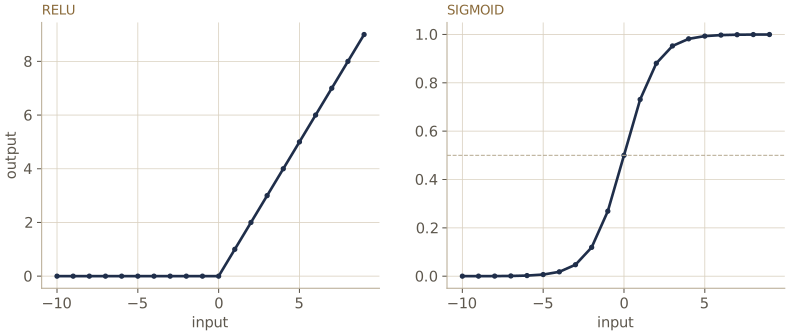
\[\text{ReLU}(x) = \max(0,\, x)\]It leaves positive numbers alone and turns negative numbers into 0. That tiny kink at zero is enough: with enough ReLU units, a network can build a boundary out of many short straight pieces, bent wherever it needs.
A model with non-linearity
We take model_1’s architecture and insert nn.ReLU() between the layers. Only the hidden layers get an activation; the output layer produces logits, and the sigmoid is applied in the loss function (training) and by us (predictions).
class CircleModelV2(nn.Module):
    def __init__(self):
        super().__init__()
        self.layer_1 = nn.Linear(in_features=2, out_features=10)
        self.layer_2 = nn.Linear(in_features=10, out_features=10)
        self.layer_3 = nn.Linear(in_features=10, out_features=1)
        self.relu = nn.ReLU()   # the non-linear activation

    def forward(self, x):
        # ReLU between the layers, none after the last one
        return self.layer_3(self.relu(self.layer_2(self.relu(self.layer_1(x)))))

torch.manual_seed(42)
model_3 = CircleModelV2().to(device)
model_3
CircleModelV2(
  (layer_1): Linear(in_features=2, out_features=10, bias=True)
  (layer_2): Linear(in_features=10, out_features=10, bias=True)
  (layer_3): Linear(in_features=10, out_features=1, bias=True)
  (relu): ReLU()
)
Training the non-linear model
Everything else stays as it was for model_1 — same loss, optimizer, and learning rate. We do train for longer, 2,000 epochs instead of 1,000, printing every 200; for a fair comparison with model_1, look at the line for epoch 1,000, where only the activations differ.
loss_fn = nn.BCEWithLogitsLoss()
optimizer = torch.optim.SGD(params=model_3.parameters(), lr=0.1)

torch.manual_seed(42)
epochs = 2000

for epoch in range(epochs):
    model_3.train()
    y_logits = model_3(X_train).squeeze()
    y_pred = torch.round(torch.sigmoid(y_logits))
    loss = loss_fn(y_logits, y_train)
    acc = accuracy_fn(y_true=y_train, y_pred=y_pred)
    optimizer.zero_grad()
    loss.backward()
    optimizer.step()

    model_3.eval()
    with torch.inference_mode():
        test_logits = model_3(X_test).squeeze()
        test_pred = torch.round(torch.sigmoid(test_logits))
        test_loss = loss_fn(test_logits, y_test)
        test_acc = accuracy_fn(y_true=y_test, y_pred=test_pred)

    if epoch % 200 == 0:
        print(f"Epoch: {epoch:4d} | Loss: {loss:.5f}, Acc: {acc:.2f}% "
              f"| Test loss: {test_loss:.5f}, Test acc: {test_acc:.2f}%")
Epoch:    0 | Loss: 0.69295, Acc: 50.00% | Test loss: 0.69319, Test acc: 50.00%
Epoch:  200 | Loss: 0.68977, Acc: 53.37% | Test loss: 0.68940, Test acc: 55.00%
Epoch:  400 | Loss: 0.68517, Acc: 52.75% | Test loss: 0.68411, Test acc: 56.50%
Epoch:  600 | Loss: 0.67515, Acc: 54.50% | Test loss: 0.67285, Test acc: 56.00%
Epoch:  800 | Loss: 0.65160, Acc: 64.00% | Test loss: 0.64757, Test acc: 67.50%
Epoch: 1000 | Loss: 0.56818, Acc: 87.75% | Test loss: 0.57378, Test acc: 86.50%
Epoch: 1200 | Loss: 0.37056, Acc: 97.75% | Test loss: 0.40595, Test acc: 92.00%
Epoch: 1400 | Loss: 0.17180, Acc: 99.50% | Test loss: 0.22108, Test acc: 97.50%
Epoch: 1600 | Loss: 0.09123, Acc: 99.88% | Test loss: 0.12741, Test acc: 99.50%
Epoch: 1800 | Loss: 0.05773, Acc: 99.88% | Test loss: 0.08672, Test acc: 99.50%
For the first few hundred epochs little happens — the loss creeps down while the model finds a useful direction. Then it takes off. At epoch 1,000, where model_1 stopped at around 46% test accuracy, this model is already at 86.5% — the activations alone made that difference. It was still well short of its best, though: the loss was still falling fast, which is the signal to train longer.
Evaluating the non-linear model
model_3.eval()
with torch.inference_mode():
    y_preds = torch.round(torch.sigmoid(model_3(X_test))).squeeze()

print(f"Predictions: {y_preds[:10]}")
print(f"Labels:      {y_test[:10]}")
print(f"Test accuracy: {accuracy_fn(y_true=y_test, y_pred=y_preds):.2f}%")
Predictions: tensor([1., 0., 1., 0., 1., 1., 0., 0., 1., 0.])
Labels:      tensor([1., 0., 1., 0., 1., 1., 0., 0., 1., 0.])
Test accuracy: 100.00%
After the full 2,000 epochs (the last printed line was epoch 1,800, at 99.5%), the model classifies every one of the 200 test points correctly.
plt.figure(figsize=(12, 5))
plt.subplot(1, 2, 1)
plt.title("Train")
plot_decision_boundary(model_3, X_train, y_train)
plt.subplot(1, 2, 2)
plt.title("Test")
plot_decision_boundary(model_3, X_test, y_test)
plt.show()
The right panel of the decision-boundary figure in step 4 shows the result: a closed boundary around the inner circle. Compared with model_1, the ReLU activations are the only change to the model, and they made the difference between guessing and solving the problem.
Note. A neural network is a stack of linear layers (straight lines) and non-linear activations (bends). Give it both, and enough data, and it can learn patterns that nobody wrote down. That sentence summarizes most of deep learning.
Replicating the activation functions
Activation functions are not magic; each is a line of arithmetic. Let’s rebuild ReLU and sigmoid by hand and check them against PyTorch’s versions.
A = torch.arange(-10, 10, 1, dtype=torch.float32)
A
tensor([-10.,  -9.,  -8.,  -7.,  -6.,  -5.,  -4.,  -3.,  -2.,  -1.,   0.,   1.,
          2.,   3.,   4.,   5.,   6.,   7.,   8.,   9.])
ReLU keeps the larger of 0 and each input:
def relu(x):
    return torch.maximum(torch.tensor(0), x)

print(relu(A))
print(torch.equal(relu(A), torch.relu(A)))
tensor([0., 0., 0., 0., 0., 0., 0., 0., 0., 0., 0., 1., 2., 3., 4., 5., 6., 7.,
        8., 9.])
True
Sigmoid is the formula from earlier, \(1 / (1 + e^{-x})\):
def sigmoid(x):
    return 1 / (1 + torch.exp(-x))

# a few values: far left (-10), around zero (-1, 0, 1), far right (9)
print(sigmoid(A)[[0, 9, 10, 11, 19]])
print(torch.allclose(sigmoid(A), torch.sigmoid(A)))
tensor([4.5398e-05, 2.6894e-01, 5.0000e-01, 7.3106e-01, 9.9988e-01])
True
Our hand-written versions agree with PyTorch’s. (allclose allows for tiny rounding differences, which is the right way to compare floating-point results.) Plot relu(A) and sigmoid(A) against A to reproduce the activation figure above:
plt.figure(figsize=(10, 4))
plt.subplot(1, 2, 1)
plt.plot(A, relu(A))
plt.subplot(1, 2, 2)
plt.plot(A, sigmoid(A))
plt.show()
Multi-class classification
Now for more than two classes. The recipe changes in three places, all at the end of the model: one output per class, softmax instead of sigmoid, and cross entropy as the loss.
Data: four blobs
make_blobs scatters points around several centers. We make 4 classes of 2-D points:
from sklearn.datasets import make_blobs

NUM_CLASSES = 4
NUM_FEATURES = 2
RANDOM_SEED = 42

X_blob, y_blob = make_blobs(n_samples=1000, n_features=NUM_FEATURES,
                            centers=NUM_CLASSES, cluster_std=1.5,
                            random_state=RANDOM_SEED)

X_blob = torch.from_numpy(X_blob).type(torch.float32)
y_blob = torch.from_numpy(y_blob).type(torch.long)   # class labels are integers

X_blob_train, X_blob_test, y_blob_train, y_blob_test = train_test_split(
    X_blob, y_blob, test_size=0.2, random_state=RANDOM_SEED)

print(X_blob_train.shape, y_blob_train.shape)
print(y_blob_train[:10])
torch.Size([800, 2]) torch.Size([800])
tensor([1, 0, 2, 2, 0, 0, 0, 1, 3, 0])
Two details. The labels are now whole numbers 0, 1, 2, 3, stored as torch.long (64-bit integers) — that is the type CrossEntropyLoss expects. And cluster_std=1.5 spreads the points of each blob, so that some blobs come close to each other.
plt.figure(figsize=(8, 5))
plt.scatter(X_blob[:, 0], X_blob[:, 1], c=y_blob, cmap=plt.cm.RdYlBu, s=10)
plt.show()
A multi-class model
The model has NUM_CLASSES outputs — one logit per class. We write it with an nn.Sequential block inside an nn.Module, and let the caller choose the sizes:
class BlobModel(nn.Module):
    def __init__(self, input_features, output_features, hidden_units=8):
        """
        input_features:  number of input features
        output_features: number of classes
        hidden_units:    number of hidden units between layers
        """
        super().__init__()
        self.linear_layer_stack = nn.Sequential(
            nn.Linear(in_features=input_features, out_features=hidden_units),
            nn.Linear(in_features=hidden_units, out_features=hidden_units),
            nn.Linear(in_features=hidden_units, out_features=output_features)
        )

    def forward(self, x):
        return self.linear_layer_stack(x)

torch.manual_seed(42)
model_4 = BlobModel(input_features=NUM_FEATURES,
                    output_features=NUM_CLASSES).to(device)
model_4
BlobModel(
  (linear_layer_stack): Sequential(
    (0): Linear(in_features=2, out_features=8, bias=True)
    (1): Linear(in_features=8, out_features=8, bias=True)
    (2): Linear(in_features=8, out_features=4, bias=True)
  )
)
We left out the ReLUs on purpose. Look at the plot of the blobs: straight lines might be enough to separate them. We will see whether a linear model can manage.
Softmax and cross entropy
Each sample now gets four logits:
X_blob_train, y_blob_train = X_blob_train.to(device), y_blob_train.to(device)
X_blob_test, y_blob_test = X_blob_test.to(device), y_blob_test.to(device)

model_4.eval()
with torch.inference_mode():
    y_logits = model_4(X_blob_test)

y_logits[:5]
tensor([[-1.2549, -0.8112, -1.4795, -0.5696],
        [ 1.7168, -1.2270,  1.7367,  2.1010],
        [ 2.2400,  0.7714,  2.6020,  1.0107],
        [-0.7993, -0.3723, -0.9138, -0.5388],
        [-0.4332, -1.6117, -0.6891,  0.6852]])
To turn them into probabilities we use softmax, which exponentiates each logit and divides by the total:
\[\text{softmax}(z)_k = \frac{e^{z_k}}{\sum_{j} e^{z_j}}\]Every result is between 0 and 1, and the probabilities for one sample add up to 1. The predicted class is the position of the largest probability, found with argmax:
y_pred_probs = torch.softmax(y_logits, dim=1)   # across the classes of each sample
print(y_pred_probs[:5])
print(f"Sum of the first row: {y_pred_probs[0].sum():.4f}")
print(f"Predicted classes: {y_pred_probs.argmax(dim=1)[:5]}")
print(f"True classes:      {y_blob_test[:5]}")
tensor([[0.1872, 0.2918, 0.1495, 0.3715],
        [0.2824, 0.0149, 0.2881, 0.4147],
        [0.3380, 0.0778, 0.4854, 0.0989],
        [0.2118, 0.3246, 0.1889, 0.2748],
        [0.1945, 0.0598, 0.1506, 0.5951]])
Sum of the first row: 1.0000
Predicted classes: tensor([3, 3, 2, 1, 3])
True classes:      tensor([1, 3, 2, 1, 0])
dim=1 matters: the tensor has shape [200, 4] (samples × classes), and we want the probabilities across the 4 classes of each sample, so we normalize along dimension 1. Logits → softmax → argmax is the multi-class version of logits → sigmoid → round.
The multi-class loss is cross entropy. It is the negative log of the probability the model assigns to the true class, averaged over the samples:
\[\text{CE} = -\frac{1}{n}\sum_{i=1}^{n} \log p_{i,\,y_i}\]nn.CrossEntropyLoss takes raw logits (it applies softmax internally, for the same stability reason as BCEWithLogitsLoss) and integer class labels.
loss_fn = nn.CrossEntropyLoss()
optimizer = torch.optim.SGD(params=model_4.parameters(), lr=0.1)
Training and testing
torch.manual_seed(42)
epochs = 100

for epoch in range(epochs):
    model_4.train()
    y_logits = model_4(X_blob_train)                     # [800, 4], no squeeze needed
    y_pred = torch.softmax(y_logits, dim=1).argmax(dim=1)
    loss = loss_fn(y_logits, y_blob_train)
    acc = accuracy_fn(y_true=y_blob_train, y_pred=y_pred)
    optimizer.zero_grad()
    loss.backward()
    optimizer.step()

    model_4.eval()
    with torch.inference_mode():
        test_logits = model_4(X_blob_test)
        test_pred = torch.softmax(test_logits, dim=1).argmax(dim=1)
        test_loss = loss_fn(test_logits, y_blob_test)
        test_acc = accuracy_fn(y_true=y_blob_test, y_pred=test_pred)

    if epoch % 10 == 0:
        print(f"Epoch: {epoch:3d} | Loss: {loss:.5f}, Acc: {acc:.2f}% "
              f"| Test loss: {test_loss:.5f}, Test acc: {test_acc:.2f}%")
Epoch:   0 | Loss: 1.04324, Acc: 65.50% | Test loss: 0.57861, Test acc: 95.50%
Epoch:  10 | Loss: 0.14398, Acc: 99.12% | Test loss: 0.13037, Test acc: 99.00%
Epoch:  20 | Loss: 0.08062, Acc: 99.12% | Test loss: 0.07216, Test acc: 99.50%
Epoch:  30 | Loss: 0.05924, Acc: 99.12% | Test loss: 0.05133, Test acc: 99.50%
Epoch:  40 | Loss: 0.04892, Acc: 99.00% | Test loss: 0.04098, Test acc: 99.50%
Epoch:  50 | Loss: 0.04295, Acc: 99.00% | Test loss: 0.03486, Test acc: 99.50%
Epoch:  60 | Loss: 0.03910, Acc: 99.00% | Test loss: 0.03083, Test acc: 99.50%
Epoch:  70 | Loss: 0.03643, Acc: 99.00% | Test loss: 0.02799, Test acc: 99.50%
Epoch:  80 | Loss: 0.03448, Acc: 99.00% | Test loss: 0.02587, Test acc: 99.50%
Epoch:  90 | Loss: 0.03300, Acc: 99.12% | Test loss: 0.02423, Test acc: 99.50%
The model learns quickly and reaches high accuracy on both sets. The output has one column per class already, so there is nothing to squeeze.
Predictions and decision boundaries
model_4.eval()
with torch.inference_mode():
    y_logits = model_4(X_blob_test)
y_preds = torch.softmax(y_logits, dim=1).argmax(dim=1)

print(f"Predictions: {y_preds[:10]}")
print(f"Labels:      {y_blob_test[:10]}")
print(f"Test accuracy: {accuracy_fn(y_true=y_blob_test, y_pred=y_preds):.2f}%")
Predictions: tensor([1, 3, 2, 1, 0, 3, 2, 0, 2, 0])
Labels:      tensor([1, 3, 2, 1, 0, 3, 2, 0, 2, 0])
Test accuracy: 99.50%
plt.figure(figsize=(12, 5))
plt.subplot(1, 2, 1)
plt.title("Train")
plot_decision_boundary(model_4, X_blob_train, y_blob_train)
plt.subplot(1, 2, 2)
plt.title("Test")
plot_decision_boundary(model_4, X_blob_test, y_blob_test)
plt.show()
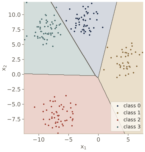
The boundaries are straight, as they must be for a model without activations, and that suffices here. Whether a model needs non-linearity depends on the data; the circles did, the blobs do not.
More ways to measure a classifier
Accuracy is easy to read, but it can mislead. Suppose 1 weld in 100 is defective. A “model” that always answers good is 99% accurate — and catches none of the defects. The metrics below look at the kinds of mistakes a model makes.
For one class of interest (the positive class, say defective), every prediction falls into one of four boxes:
- True positive (TP): predicted defective, is defective.
- False positive (FP): predicted defective, is good — a false alarm.
- False negative (FN): predicted good, is defective — a miss.
- True negative (TN): predicted good, is good.
| Metric | Formula | Question it answers | When it matters |
|---|---|---|---|
| Accuracy | (TP + TN) / all | How often is the model right overall? | Balanced classes |
| Precision | TP / (TP + FP) | When the model says defective, how often is it right? | False alarms are costly |
| Recall | TP / (TP + FN) | Of all the defective parts, how many did it catch? | Misses are costly |
| F1 score | 2 · precision · recall / (precision + recall) | One number balancing precision and recall | Imbalanced classes |
| Confusion matrix | counts for every (true, predicted) pair | Which classes get confused with which? | Always worth a look |
Precision and recall usually pull against each other. A crack detector for a bridge should favor recall (a missed crack is dangerous); a spam filter should favor precision (losing a real email is worse than seeing some spam).
Here is the “always good” detector in code — 99 good welds (0) and 1 defective weld (1):
y_true = torch.tensor([0] * 99 + [1])
y_always_good = torch.zeros(100, dtype=torch.long)

TP = ((y_always_good == 1) & (y_true == 1)).sum().item()
FN = ((y_always_good == 0) & (y_true == 1)).sum().item()

print(f"Accuracy: {accuracy_fn(y_true, y_always_good):.0f}%")
print(f"Recall:   {TP / (TP + FN):.0f}  (defects caught: {TP} of {TP + FN})")
Accuracy: 99%
Recall:   0  (defects caught: 0 of 1)
99% accuracy, zero recall: a useless inspector.
For our multi-class model, scikit-learn computes everything in two calls. The confusion matrix has one row per true class and one column per predicted class; correct predictions lie on the diagonal. The classification report gives precision, recall, and F1 for each class:
from sklearn.metrics import confusion_matrix, classification_report

y_true_np = y_blob_test.cpu().numpy()
y_pred_np = y_preds.cpu().numpy()

print(confusion_matrix(y_true_np, y_pred_np))
print(classification_report(y_true_np, y_pred_np, digits=3))
[[49  0  0  0]
 [ 0 41  0  0]
 [ 0  0 53  0]
 [ 1  0  0 56]]
              precision    recall  f1-score   support

           0      0.980     1.000     0.990        49
           1      1.000     1.000     1.000        41
           2      1.000     1.000     1.000        53
           3      1.000     0.982     0.991        57

    accuracy                          0.995       200
   macro avg      0.995     0.996     0.995       200
weighted avg      0.995     0.995     0.995       200
Read the confusion matrix row by row: each row is a true class, and any number off the diagonal is a sample of that class predicted as another. The classification report’s support column counts how many test samples belong to each class.
Note. The library TorchMetrics computes the same metrics directly on PyTorch tensors, on the GPU if you like — for example
torchmetrics.Accuracy(task="multiclass", num_classes=4). It is worth knowing once your projects grow; scikit-learn is enough for now.
Summary
| Task | Binary | Multi-class |
|---|---|---|
| Output layer | nn.Linear(hidden, 1) |
nn.Linear(hidden, num_classes) |
| Labels | float32, 0 or 1 |
long, 0 … num_classes − 1 |
| Loss | nn.BCEWithLogitsLoss() |
nn.CrossEntropyLoss() |
| Logits → probabilities | torch.sigmoid(logits) |
torch.softmax(logits, dim=1) |
| Probabilities → labels | torch.round(probs) |
probs.argmax(dim=1) |
| Shape fix | model(X).squeeze() |
none needed |
| Hidden activation | nn.ReLU() |
nn.ReLU() (if the data needs curves) |
Other tools from this module: accuracy_fn(y_true, y_pred); nn.Sequential(...) for layers in a row; a decision-boundary plot to see what a model learned; and sklearn.metrics.confusion_matrix and classification_report for a fuller evaluation.
Three ideas to carry forward: a classifier outputs logits, and sigmoid or softmax turns them into probabilities; linear layers alone can only draw straight lines, so non-linear activations are what let a network learn curved patterns; and when a model fails, diagnose it with pictures and simple sanity checks, then change one thing at a time.
Exercises
- Make a binary dataset with
sklearn.datasets.make_moons(n_samples=1000, noise=0.03, random_state=42), turn it into tensors, and split it 80/20. Plot it. - Build a model for the moons data by subclassing
nn.Module, usingnn.Linearlayers with non-linear activations. - Set up
nn.BCEWithLogitsLossand an optimizer. Write a training and testing loop that prints loss and accuracy every 100 epochs, and train until test accuracy is above 96%. - Plot the decision boundary of your trained model with
plot_decision_boundary. Then remove the activations, retrain, and plot again. Describe the difference. - Replicate the tanh activation, \(\tanh(x) = (e^{x} - e^{-x}) / (e^{x} + e^{-x})\), in plain PyTorch. Check it against
torch.tanhwithtorch.allclose, and plot it next to sigmoid. How do the two differ? - Add
nn.ReLU()layers toBlobModeland retrain it on the blobs. Does it help, hurt, or make no difference? Explain from the plot of the data. - Train
model_3again with learning rates 0.01, 0.1, and 1.0, changing nothing else. Record the final test accuracy for each in a small table. - For the four-class model, write code that computes the precision and recall of class 3 by hand from the confusion matrix, and check your numbers against the classification report.
- In your own words. Describe a classification problem from your engineering field. Is it binary, multi-class, or multi-label? What would the input features be, and which matters more for it — precision or recall? Why?
Going further
- The documentation for
nn.BCEWithLogitsLossandnn.CrossEntropyLosslists their options, including class weights for imbalanced data. - The PyTorch list of non-linear activations shows the shapes of ReLU, sigmoid, tanh, and many others.
- TensorFlow Playground lets you train small networks on the circles problem in the browser and watch the decision boundary form; try it with and without activations.
- Google’s Machine Learning Crash Course: classification explains thresholds, precision, recall, and the confusion matrix with interactive examples.
These notes follow the path of Daniel Bourke's Learn PyTorch for Deep Learning (MIT license), rewritten for engineering students meeting Python and machine learning for the first time.