EAS 510 · Module 03 · Week 4
Computer Vision
Teaching a model to see — image tensors, mini-batches with DataLoader, and a small convolutional neural network.
Companion reading: Learn PyTorch for Deep Learning, chapter 03
By the end of this module you can
- Tell classification, object detection, and segmentation apart, and name an engineering use for each.
- Load an image dataset with
torchvision, read its[N, C, H, W]shape, and plot samples. - Split a dataset into shuffled mini-batches with
DataLoaderand explain why we train on batches. - Write reusable
train_step,test_step, andeval_modelfunctions and use them to train and compare several models. - Explain what a convolution, a kernel, stride, padding, and max pooling do, and trace an image’s shape through a small CNN.
- Compare models on accuracy and training time, and read a confusion matrix to see which classes a model mixes up.
- Save the best model’s weights and load them back to check they give the same results.
Contents
- What computer vision is
- Computer vision in PyTorch
- Getting a dataset: FashionMNIST
- Mini-batches with DataLoader
- Model 0: a baseline
- Evaluating a model
- Model 1: adding non-linearity
- Model 2: a convolutional neural network
- Comparing the three models
- Making predictions with the best model
- The confusion matrix
- Saving and loading the best model
- Summary
- Exercises
- Going further
In module 02 you built classifiers for points on a plane: two numbers in, a class out. This module applies the same machinery to pictures. An image is just a bigger tensor, so the loss function, optimizer, and training loop carry over almost unchanged. What changes is scale — tens of thousands of images, each with hundreds of numbers — and the kind of model that works well.
We will train three models on the same dataset of clothing photos: a plain linear baseline, a version with non-linear activations, and a small convolutional neural network (CNN), the architecture that made deep learning take off in computer vision. Along the way you will package the training loop into functions you can reuse for the rest of the course, and learn to compare models on more than a single accuracy number.
What computer vision is
Computer vision is getting a computer to extract useful information from images or video. Most problems fall into one of three shapes, which differ in what the model has to output.
| Problem | The model answers | Output | Engineering example |
|---|---|---|---|
| Classification | What is in this image? | One label per image | Is this weld good or defective? (binary) Which of six surface-defect types is on this steel sheet? (multi-class) |
| Object detection | What is where? | A box and a label for each object | Draw a box around every crack in a photo of a bridge deck |
| Segmentation | Which pixels belong to what? | A label for every pixel | Mark exactly which pixels of a pipe are corroded, so the area can be measured |
Each row asks more of the model than the one above it. This module is about classification — the foundation the other two are built on. Detection and segmentation models usually contain a classification network inside them.
You already use computer vision every day: phone cameras that sharpen faces and read documents, cars that stay in their lane, factory lines that reject faulty parts from a camera image. Wherever there is a camera and a decision to make, there is probably a vision model.
Computer vision in PyTorch
PyTorch keeps its vision tools in a companion library called torchvision. These are the pieces you will use most:
| Module | What it gives you |
|---|---|
torchvision.datasets |
Ready-made datasets for classification, detection, and more, downloaded with one line |
torchvision.models |
Well-known model architectures, optionally with weights already trained (module 06) |
torchvision.transforms |
Functions that prepare images for a model: convert to tensors, resize, flip, crop |
torch.utils.data.Dataset |
The base class for any dataset: something that returns one (image, label) pair on request |
torch.utils.data.DataLoader |
Wraps a Dataset and hands it out in shuffled mini-batches |
import torch
from torch import nn

import torchvision
from torchvision import datasets
from torchvision.transforms import ToTensor

import matplotlib.pyplot as plt

print(f"PyTorch version: {torch.__version__}")
print(f"torchvision version: {torchvision.__version__}")

device = "cuda" if torch.cuda.is_available() else "cpu"
device
PyTorch version: 2.14.0+cu130
torchvision version: 0.29.0+cu130
'cpu'
As promised in module 00, the device line sits at the top of the notebook. Everything below moves models and data to device, so the same code runs on a laptop CPU or a Colab GPU. These notes were run on a CPU.
Getting a dataset: FashionMNIST
FashionMNIST is a set of 70,000 small grayscale photos of clothing, each 28 × 28 pixels, in 10 classes (shirts, trousers, sneakers, and so on). It was made as a harder drop-in replacement for MNIST, a famous dataset of handwritten digits. It is small enough to train on a CPU in minutes, and hard enough that model choices make a visible difference.
torchvision.datasets.FashionMNIST downloads it for us. The arguments are the same for almost every torchvision dataset:
root— the folder to download into;train—Truefor the training split,Falsefor the test split;download— fetch the files if they are not already there;transform— what to do to each image as it is loaded.ToTensor()turns a picture into a float tensor with values between 0 and 1.
train_data = datasets.FashionMNIST(
    root="data",
    train=True,
    download=True,
    transform=ToTensor(),
)

test_data = datasets.FashionMNIST(
    root="data",
    train=False,
    download=True,
    transform=ToTensor(),
)

len(train_data), len(test_data)
(60000, 10000)
Sixty thousand images to learn from and ten thousand held back for testing. Indexing the dataset returns one (image, label) pair:
image, label = train_data[0]
print(f"Image shape: {image.shape}")
print(f"Pixel values from {image.min():.1f} to {image.max():.1f}")
print(f"Label: {label}")
Image shape: torch.Size([1, 28, 28])
Pixel values from 0.0 to 1.0
Label: 9
The label is a number. The dataset also carries the class names, in the same order:
class_names = train_data.classes
class_names
['T-shirt/top', 'Trouser', 'Pullover', 'Dress', 'Coat', 'Sandal', 'Shirt', 'Sneaker', 'Bag', 'Ankle boot']
So label 9 means Ankle boot.
Image tensors and the NCHW convention
The image came out with shape [1, 28, 28]. The three numbers are
- color channels — 1 for grayscale; 3 for a color photo (red, green, blue);
- height — 28 rows of pixels;
- width — 28 columns.
This order, channels first, is written CHW. When we feed a model many images at once, a batch dimension goes in front, giving NCHW: [batch_size, color_channels, height, width]. A batch of 32 FashionMNIST images is [32, 1, 28, 28]; a batch of 32 color photos at 224 × 224 is [32, 3, 224, 224].
Image files and plotting libraries such as matplotlib use the other order, channels last — NHWC or [height, width, channels]. You met permute in module 00 for converting between the two. PyTorch layers expect channels first, so that is what we use.
Note. Channels-last can run faster on some GPUs, and PyTorch supports it as a memory-format option. You will not need it in this course, but you will see both orders in other people’s code, so check the shape before you assume.
Looking at the data
Always look at your data before modeling it. matplotlib’s imshow expects [height, width] for a grayscale image, so we squeeze away the channel dimension:
image, label = train_data[0]
plt.imshow(image.squeeze(), cmap="gray")
plt.title(class_names[label])
plt.axis(False);
To see more than one, draw a grid of random samples:
torch.manual_seed(42)
fig = plt.figure(figsize=(9, 9))
rows, cols = 4, 4
for i in range(1, rows * cols + 1):
    random_idx = torch.randint(0, len(train_data), size=[1]).item()
    img, label = train_data[random_idx]
    fig.add_subplot(rows, cols, i)
    plt.imshow(img.squeeze(), cmap="gray")
    plt.title(class_names[label])
    plt.axis(False);
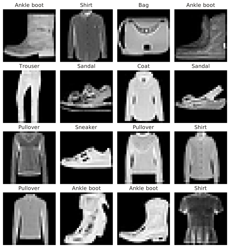
Could a hand-written rule tell these apart? Perhaps “bright pixels only at the bottom means a shoe” — but rules like that break on the next image. This is the situation from module 00 where learning the rules from examples pays off.
Mini-batches with DataLoader
So far the data is a Python list-like Dataset of 60,000 pairs. We could push all 60,000 images through the model at once, compute one loss, and take one optimizer step. We don’t, for two reasons.
- Memory. A real dataset of large images does not fit in GPU memory in one go.
- More updates. One step per pass over the data is slow learning. If we split the data into small groups — mini-batches — and update the weights after each one, the model gets 1,875 chances to improve per pass instead of one.
The number of images in each mini-batch is the batch size. It is a hyperparameter (module 01): a setting you choose, as opposed to a parameter the model learns. Powers of two such as 32, 64, and 128 are the usual choices; 32 is a sound default. One full pass over the training data is still an epoch.
DataLoader does the batching. Its shuffle=True option mixes the order of the training images every epoch, so the model does not learn anything from the order the files happen to be in (all the sneakers first, say). There is no need to shuffle the test data, since we never learn from it.
from torch.utils.data import DataLoader

BATCH_SIZE = 32

train_dataloader = DataLoader(train_data, batch_size=BATCH_SIZE, shuffle=True)
test_dataloader = DataLoader(test_data, batch_size=BATCH_SIZE, shuffle=False)

print(f"Train batches: {len(train_dataloader)} of {BATCH_SIZE} images")
print(f"Test batches:  {len(test_dataloader)} of {BATCH_SIZE} images")
Train batches: 1875 of 32 images
Test batches:  313 of 32 images
A DataLoader is an iterable: you loop over it, or take one batch with next(iter(...)):
train_features_batch, train_labels_batch = next(iter(train_dataloader))
train_features_batch.shape, train_labels_batch.shape
(torch.Size([32, 1, 28, 28]), torch.Size([32]))
There is the NCHW shape: 32 images, 1 channel, 28 × 28 pixels, and 32 labels to go with them.
Model 0: a baseline
A baseline is the simplest model worth trying. Its job is not to be good but to give you a number to beat. Every later, more complicated model has to justify itself against it.
Flattening an image
A linear layer (nn.Linear) expects each example to be a vector — a single row of numbers. An image is a grid. nn.Flatten() joins the rows of the grid end to end:
flatten_model = nn.Flatten()

x = train_features_batch[0]
output = flatten_model(x)

print(f"Before flattening: {x.shape}  -> [color_channels, height, width]")
print(f"After flattening:  {output.shape}  -> [color_channels, height*width]")
Before flattening: torch.Size([1, 28, 28])  -> [color_channels, height, width]
After flattening:  torch.Size([1, 784])  -> [color_channels, height*width]
28 × 28 = 784 numbers per image. Flattening keeps every pixel value but throws away which pixel was next to which — hold on to that thought.
Building the model
Model 0 is a flatten layer followed by two linear layers, with no activation functions between them:
class FashionMNISTModelV0(nn.Module):
    def __init__(self, input_shape: int, hidden_units: int, output_shape: int):
        super().__init__()
        self.layer_stack = nn.Sequential(
            nn.Flatten(),                    # [N, 1, 28, 28] -> [N, 784]
            nn.Linear(in_features=input_shape, out_features=hidden_units),
            nn.Linear(in_features=hidden_units, out_features=output_shape),
        )

    def forward(self, x):
        return self.layer_stack(x)

torch.manual_seed(42)
model_0 = FashionMNISTModelV0(input_shape=784,       # 28 * 28 pixels
                              hidden_units=10,       # hidden layer width
                              output_shape=len(class_names)).to(device)
model_0
FashionMNISTModelV0(
  (layer_stack): Sequential(
    (0): Flatten(start_dim=1, end_dim=-1)
    (1): Linear(in_features=784, out_features=10, bias=True)
    (2): Linear(in_features=10, out_features=10, bias=True)
  )
)
hidden_units=10 is another hyperparameter — the width of the hidden layer. The output layer produces ten numbers per image, one logit per class, just as in the multi-class model of module 02.
Loss, optimizer, and accuracy
This is multi-class classification, so the setup is the one from module 02: nn.CrossEntropyLoss for the loss, stochastic gradient descent for the optimizer, and accuracy as a number people can read.
def accuracy_fn(y_true, y_pred):
    """Percentage of predictions that match the labels."""
    correct = torch.eq(y_true, y_pred).sum().item()
    return (correct / len(y_pred)) * 100

loss_fn = nn.CrossEntropyLoss()
optimizer = torch.optim.SGD(params=model_0.parameters(), lr=0.1)
Timing experiments
Accuracy is not the only thing that matters. A model that is 1% better but takes ten times longer to train (or to make a prediction) may not be worth it. A small helper records the wall-clock time of each training run:
from timeit import default_timer as timer

def print_train_time(start: float, end: float, device=None):
    """Print and return the time between start and end, in seconds."""
    total_time = end - start
    print(f"Train time on {device}: {total_time:.1f} seconds")
    return total_time
A training loop over batches
The loop is the one from modules 01 and 02 with one more level: for each epoch, we now loop over the batches, and take an optimizer step after each batch. Loss and accuracy are added up batch by batch and divided by the number of batches at the end, giving the average per batch for that epoch.
torch.manual_seed(42)
train_time_start_model_0 = timer()

epochs = 3

for epoch in range(epochs):
    # --- Training ---
    train_loss = 0
    model_0.train()
    for X, y in train_dataloader:
        X, y = X.to(device), y.to(device)
        y_pred = model_0(X)                      # 1. forward pass
        loss = loss_fn(y_pred, y)                # 2. loss for this batch
        train_loss += loss.item()
        optimizer.zero_grad()                    # 3. clear old gradients
        loss.backward()                          # 4. backpropagation
        optimizer.step()                         # 5. update weights (every batch)
    train_loss /= len(train_dataloader)

    # --- Testing ---
    test_loss, test_acc = 0, 0
    model_0.eval()
    with torch.inference_mode():
        for X, y in test_dataloader:
            X, y = X.to(device), y.to(device)
            test_pred = model_0(X)
            test_loss += loss_fn(test_pred, y).item()
            test_acc += accuracy_fn(y_true=y, y_pred=test_pred.argmax(dim=1))
        test_loss /= len(test_dataloader)
        test_acc /= len(test_dataloader)

    print(f"Epoch {epoch} | Train loss: {train_loss:.4f} | "
          f"Test loss: {test_loss:.4f} | Test acc: {test_acc:.2f}%")

train_time_end_model_0 = timer()
total_train_time_model_0 = print_train_time(start=train_time_start_model_0,
                                            end=train_time_end_model_0,
                                            device=device)
Epoch 0 | Train loss: 0.5904 | Test loss: 0.5095 | Test acc: 82.04%
Epoch 1 | Train loss: 0.4763 | Test loss: 0.4799 | Test acc: 83.20%
Epoch 2 | Train loss: 0.4550 | Test loss: 0.4766 | Test acc: 83.43%
Train time on cpu: 81.0 seconds
Three things to notice. The test loss fell each epoch, so the model is learning. After three passes the baseline gets around four images in five right — far better than the 10% of guessing at random. And training took a minute or two on a CPU. That accuracy is the bar to beat.
We used test_pred.argmax(dim=1) rather than a softmax followed by an argmax. Softmax never changes which logit is largest, so for picking a class it can be skipped.
Evaluating a model
We will train several models and want to compare them fairly, on the same data and the same measures. A function makes that one line per model. eval_model runs a model over a whole DataLoader in inference mode and returns a dictionary:
def eval_model(model: torch.nn.Module,
               data_loader: torch.utils.data.DataLoader,
               loss_fn: torch.nn.Module,
               accuracy_fn,
               device: torch.device = device):
    """Return the model's name, average loss, and accuracy on data_loader."""
    loss, acc = 0, 0
    model.eval()
    with torch.inference_mode():
        for X, y in data_loader:
            X, y = X.to(device), y.to(device)
            y_pred = model(X)
            loss += loss_fn(y_pred, y).item()
            acc += accuracy_fn(y_true=y, y_pred=y_pred.argmax(dim=1))
        loss /= len(data_loader)
        acc /= len(data_loader)
    return {"model_name": model.__class__.__name__,
            "model_loss": loss,
            "model_acc": acc}

model_0_results = eval_model(model=model_0, data_loader=test_dataloader,
                             loss_fn=loss_fn, accuracy_fn=accuracy_fn,
                             device=device)
model_0_results
{'model_name': 'FashionMNISTModelV0', 'model_loss': 0.4766388931118261, 'model_acc': 83.42651757188499}
The numbers match the last epoch above, as they should: same model, same test data.
Model 1: adding non-linearity
In module 02, adding nn.ReLU() between linear layers is what let a model bend its decision boundary around circles. Maybe images need the same. Model 1 is model 0 with a ReLU after each linear layer:
class FashionMNISTModelV1(nn.Module):
    def __init__(self, input_shape: int, hidden_units: int, output_shape: int):
        super().__init__()
        self.layer_stack = nn.Sequential(
            nn.Flatten(),
            nn.Linear(in_features=input_shape, out_features=hidden_units),
            nn.ReLU(),
            nn.Linear(in_features=hidden_units, out_features=output_shape),
            nn.ReLU(),
        )

    def forward(self, x: torch.Tensor):
        return self.layer_stack(x)

torch.manual_seed(42)
model_1 = FashionMNISTModelV1(input_shape=784,
                              hidden_units=10,
                              output_shape=len(class_names)).to(device)

loss_fn = nn.CrossEntropyLoss()
optimizer = torch.optim.SGD(params=model_1.parameters(), lr=0.1)
Turning the loops into functions
We are about to write the same training and testing loops a second and third time. Instead, put each in a function. These two functions, together with eval_model, are the reusable core of this module; module 04 extends them and module 05 moves them into a file.
train_steptrains a model for one epoch — one pass over aDataLoader.test_stepevaluates it for one epoch, without changing any weights.
def train_step(model: torch.nn.Module,
               data_loader: torch.utils.data.DataLoader,
               loss_fn: torch.nn.Module,
               optimizer: torch.optim.Optimizer,
               accuracy_fn,
               device: torch.device = device):
    """Train model for one epoch and print the average loss and accuracy."""
    train_loss, train_acc = 0, 0
    model.train()
    for X, y in data_loader:
        X, y = X.to(device), y.to(device)
        y_pred = model(X)                                   # 1. forward pass
        loss = loss_fn(y_pred, y)                           # 2. loss
        train_loss += loss.item()
        train_acc += accuracy_fn(y_true=y, y_pred=y_pred.argmax(dim=1))
        optimizer.zero_grad()                               # 3. zero the gradients
        loss.backward()                                     # 4. backpropagation
        optimizer.step()                                    # 5. update the weights
    train_loss /= len(data_loader)
    train_acc /= len(data_loader)
    print(f"Train loss: {train_loss:.4f} | Train accuracy: {train_acc:.2f}%")


def test_step(model: torch.nn.Module,
              data_loader: torch.utils.data.DataLoader,
              loss_fn: torch.nn.Module,
              accuracy_fn,
              device: torch.device = device):
    """Evaluate model for one epoch and print the average loss and accuracy."""
    test_loss, test_acc = 0, 0
    model.eval()
    with torch.inference_mode():
        for X, y in data_loader:
            X, y = X.to(device), y.to(device)
            test_pred = model(X)
            test_loss += loss_fn(test_pred, y).item()
            test_acc += accuracy_fn(y_true=y, y_pred=test_pred.argmax(dim=1))
        test_loss /= len(data_loader)
        test_acc /= len(data_loader)
    print(f"Test loss:  {test_loss:.4f} | Test accuracy:  {test_acc:.2f}%")
Every argument the loop needs comes in through the function’s parameters — the model, the data, the loss, the optimizer, the device — so the same functions work for any classification model. Training model 1 is now short:
torch.manual_seed(42)
train_time_start_model_1 = timer()

epochs = 3
for epoch in range(epochs):
    print(f"Epoch {epoch}")
    train_step(model=model_1, data_loader=train_dataloader, loss_fn=loss_fn,
               optimizer=optimizer, accuracy_fn=accuracy_fn, device=device)
    test_step(model=model_1, data_loader=test_dataloader, loss_fn=loss_fn,
              accuracy_fn=accuracy_fn, device=device)

train_time_end_model_1 = timer()
total_train_time_model_1 = print_train_time(start=train_time_start_model_1,
                                            end=train_time_end_model_1,
                                            device=device)
Epoch 0
Train loss: 1.0920 | Train accuracy: 61.34%
Test loss:  0.9564 | Test accuracy:  65.00%
Epoch 1
Train loss: 0.7810 | Train accuracy: 71.93%
Test loss:  0.7223 | Test accuracy:  73.91%
Epoch 2
Train loss: 0.6703 | Train accuracy: 75.94%
Test loss:  0.6850 | Test accuracy:  75.02%
Train time on cpu: 109.0 seconds
model_1_results = eval_model(model=model_1, data_loader=test_dataloader,
                             loss_fn=loss_fn, accuracy_fn=accuracy_fn,
                             device=device)
model_1_results
{'model_name': 'FashionMNISTModelV1', 'model_loss': 0.685000919971984, 'model_acc': 75.01996805111821}
Why model 1 is not better
Adding non-linearity made things worse: about 75% test accuracy against the baseline’s 83%, and a higher loss. Look at the training accuracy too — it is also around 76%. The model is not even fitting the data it trains on, so this is not memorization of the training set; the model is struggling to learn at all. This is underfitting, which you met with the circles in module 02; module 04 treats it in detail. Two features of the design are likely culprits:
- The ReLU after the last layer. It turns every negative logit into zero, so the model cannot push the score of a wrong class below zero, and the gradient through those zeroed outputs is zero, so they stop learning. Output layers of classifiers normally have no activation; the softmax inside the loss function does that job.
- A narrow hidden layer. Ten hidden units must carry everything the model knows about the image. A ReLU sets some of them to zero for many inputs, and whatever information they carried is lost.
More epochs or a wider hidden layer might close the gap (exercise 6 asks you to test the first cause). But even the best version of this model has a deeper problem, which the next model addresses.
This is a common experience, and a useful one: adding complexity does not guarantee improvement. The only way to know whether a change helps is to run the experiment and compare against the baseline. Keep that habit; module 07 is built around it.
Model 2: a convolutional neural network
Both models so far start by flattening the image into a row of 784 numbers. After that, the model has no idea that pixel 29 sits directly below pixel 1. Yet in a picture, what matters is local structure: edges, corners, and textures, formed by neighboring pixels. A convolutional neural network (CNN) is designed around this. Instead of looking at all pixels at once, it slides small learned filters over the image and responds wherever a pattern appears.
Which kind of model for which kind of data
A rough guide, with plenty of exceptions:
| Data | Typical models | Where to find them |
|---|---|---|
| Structured — rows and columns, like a spreadsheet of sensor readings | Gradient-boosted trees, random forests | scikit-learn, XGBoost |
| Unstructured — images, audio, text | Convolutional neural networks, transformers | torchvision.models, Hugging Face Transformers |
The model we build is TinyVGG, the small CNN used by the interactive CNN Explainer website. Its layout is the classic one:
input → [convolution → activation → pooling] → [convolution → activation → pooling] → classifier → output
The bracketed blocks can be repeated and widened; much larger CNNs follow the same plan. Before building it, let us look at each new layer on its own.
Convolution: a kernel sliding over the image
A convolutional layer holds a few small grids of weights called kernels (or filters), typically 3 × 3. To apply a kernel, place it over a 3 × 3 patch of the image, multiply each image value by the kernel weight on top of it, and add up the nine products (plus a bias). That sum is one number of the output. Then slide the kernel one step along and repeat, until it has visited every position.
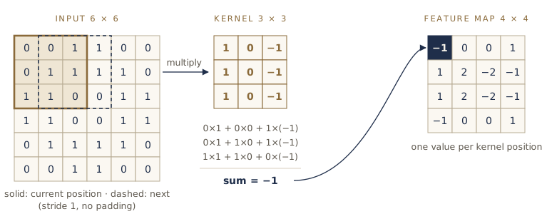
The grid of outputs is called a feature map: it shows where in the image the kernel’s pattern appears. The kernel in the figure was chosen by hand to detect vertical edges. In a CNN nobody chooses the kernel values — they are weights, and gradient descent learns them, just like the weights of a linear layer. Early layers typically end up with edge and color detectors; later layers combine those into textures and shapes.
A layer usually has several kernels, each producing its own feature map. Those maps are stacked as the channels of the output. So a layer with 10 kernels turns a 1-channel image into a 10-channel stack of feature maps. With a color image, each kernel spans all three input channels (it is 3 × 3 × 3) and still produces one feature map.
Three hyperparameters control the sliding:
- kernel_size — the size of the kernel.
kernel_size=3means 3 × 3. - stride — how many pixels the kernel moves per step. With
stride=2it skips every other position and the output is about half the size. - padding — a border of zeros added around the input. Without padding, a 3 × 3 kernel cannot be centered on the edge pixels, so the output shrinks by 2 in each direction (6 × 6 → 4 × 4 in the figure).
padding=1adds one ring of zeros and keeps the output the same size as the input.
For an input of height \(H\), kernel size \(K\), padding \(P\), and stride \(S\), the output height is
\[H_{\text{out}} = \left\lfloor \frac{H + 2P - K}{S} \right\rfloor + 1\]and the same for the width. (\(\lfloor\cdot\rfloor\) means round down.) Check it on the figure: \(\lfloor (6 + 0 - 3)/1 \rfloor + 1 = 4\).
In PyTorch the layer is nn.Conv2d (“2d” because the kernel slides in two directions, across and down). Try it on a batch of random “images” shaped like color photos:
torch.manual_seed(42)
images = torch.randn(size=(32, 3, 64, 64))   # [batch_size, channels, height, width]
test_image = images[0]

print(f"Image batch shape:  {images.shape}")
print(f"Single image shape: {test_image.shape}")
Image batch shape:  torch.Size([32, 3, 64, 64])
Single image shape: torch.Size([3, 64, 64])
torch.manual_seed(42)
conv_layer = nn.Conv2d(in_channels=3,    # color channels coming in
                       out_channels=10,  # number of kernels = feature maps out
                       kernel_size=3,
                       stride=1,
                       padding=0)

conv_layer(test_image.unsqueeze(dim=0)).shape
torch.Size([1, 10, 62, 62])
We added a batch dimension with unsqueeze(dim=0) to make the single image [1, 3, 64, 64]. Out came 10 feature maps, each 62 × 62: without padding the size shrank by 2, exactly as the formula says. Now change the settings:
torch.manual_seed(42)
conv_layer_2 = nn.Conv2d(in_channels=3, out_channels=10,
                         kernel_size=(5, 5), stride=2, padding=0)

conv_layer_2(test_image.unsqueeze(dim=0)).shape
torch.Size([1, 10, 30, 30])
With a 5 × 5 kernel and stride 2: \(\lfloor (64 - 5)/2 \rfloor + 1 = 30\). The learned weights live where you would expect:
# weight shape: [out_channels, in_channels, kernel_height, kernel_width]
print(f"Kernel weights shape: {conv_layer_2.weight.shape}")
print(f"Bias shape:           {conv_layer_2.bias.shape}")
Kernel weights shape: torch.Size([10, 3, 5, 5])
Bias shape:           torch.Size([10])
Ten kernels, each 3 × 5 × 5 (one 5 × 5 slice for each input color channel), and one bias per kernel.
ReLU
After each convolution comes a ReLU activation, the same nn.ReLU() as in module 02: negative values become zero, positive values pass through. Without it, two convolutions in a row would collapse into one bigger linear operation, and stacking layers would gain nothing.
Max pooling: shrinking the feature maps
A max pooling layer shrinks each feature map by keeping only the largest value in each small window. With nn.MaxPool2d(kernel_size=2), every 2 × 2 block of the map becomes one number, halving the height and width. Here it is on a tiny tensor so you can check it by hand:
torch.manual_seed(42)
random_tensor = torch.randn(size=(1, 1, 2, 2))
max_pool_layer = nn.MaxPool2d(kernel_size=2)
max_pool_tensor = max_pool_layer(random_tensor)

print(f"Random tensor:\n{random_tensor}")
print(f"Random tensor shape: {random_tensor.shape}")
print(f"\nMax pool tensor:\n{max_pool_tensor}")
print(f"Max pool tensor shape: {max_pool_tensor.shape}")
Random tensor:
tensor([[[[0.3367, 0.1288],
          [0.2345, 0.2303]]]])
Random tensor shape: torch.Size([1, 1, 2, 2])

Max pool tensor:
tensor([[[[0.3367]]]])
Max pool tensor shape: torch.Size([1, 1, 1, 1])
Four numbers went in and the largest one came out. Pooling has no weights to learn. Its purpose is compression: each layer summarizes the one before it in fewer numbers, keeping the strongest response in each neighborhood. It also makes the network less sensitive to exactly where a pattern appears — a feature shifted by one pixel usually lands in the same pooling window.
And on the output of our first convolution:
after_conv = conv_layer(test_image.unsqueeze(dim=0))
print(f"After conv:     {after_conv.shape}")
print(f"After max pool: {max_pool_layer(after_conv).shape}")
After conv:     torch.Size([1, 10, 62, 62])
After max pool: torch.Size([1, 10, 31, 31])
The number of channels stays at 10; height and width halve from 62 to 31.
Building TinyVGG
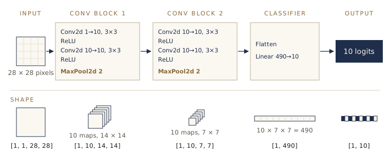
Now put the pieces together. TinyVGG has two convolutional blocks — each two Conv2d + ReLU pairs followed by a MaxPool2d — and a classifier that flattens the result and maps it to one logit per class.
in_features=490.class FashionMNISTModelV2(nn.Module):
"""TinyVGG, as used on the CNN Explainer website."""
def __init__(self, input_shape: int, hidden_units: int, output_shape: int):
super().__init__()
self.block_1 = nn.Sequential(
nn.Conv2d(in_channels=input_shape, out_channels=hidden_units,
kernel_size=3, stride=1, padding=1),
nn.ReLU(),
nn.Conv2d(in_channels=hidden_units, out_channels=hidden_units,
kernel_size=3, stride=1, padding=1),
nn.ReLU(),
nn.MaxPool2d(kernel_size=2, stride=2),
)
self.block_2 = nn.Sequential(
nn.Conv2d(hidden_units, hidden_units, kernel_size=3, padding=1),
nn.ReLU(),
nn.Conv2d(hidden_units, hidden_units, kernel_size=3, padding=1),
nn.ReLU(),
nn.MaxPool2d(2),
)
self.classifier = nn.Sequential(
nn.Flatten(),
nn.Linear(in_features=hidden_units * 7 * 7, # why 7 * 7? see below
out_features=output_shape),
)
def forward(self, x: torch.Tensor):
x = self.block_1(x)
x = self.block_2(x)
x = self.classifier(x)
return x
torch.manual_seed(42)
model_2 = FashionMNISTModelV2(input_shape=1, # grayscale: one channel
hidden_units=10, # kernels per conv layer
output_shape=len(class_names)).to(device)
model_2
FashionMNISTModelV2(
  (block_1): Sequential(
    (0): Conv2d(1, 10, kernel_size=(3, 3), stride=(1, 1), padding=(1, 1))
    (1): ReLU()
    (2): Conv2d(10, 10, kernel_size=(3, 3), stride=(1, 1), padding=(1, 1))
    (3): ReLU()
    (4): MaxPool2d(kernel_size=2, stride=2, padding=0, dilation=1, ceil_mode=False)
  )
  (block_2): Sequential(
    (0): Conv2d(10, 10, kernel_size=(3, 3), stride=(1, 1), padding=(1, 1))
    (1): ReLU()
    (2): Conv2d(10, 10, kernel_size=(3, 3), stride=(1, 1), padding=(1, 1))
    (3): ReLU()
    (4): MaxPool2d(kernel_size=2, stride=2, padding=0, dilation=1, ceil_mode=False)
  )
  (classifier): Sequential(
    (0): Flatten(start_dim=1, end_dim=-1)
    (1): Linear(in_features=490, out_features=10, bias=True)
  )
)
Here hidden_units is the number of kernels in each convolutional layer — the number of feature maps each layer produces.
Tracing the shapes layer by layer
The one number in TinyVGG you cannot write down without thinking is the classifier’s in_features. It must equal the number of values left after the last pooling layer, and that depends on the image size and every layer before it. The reliable way to find it is to push a dummy image through the layers and print the shape after each one:
dummy = torch.randn(size=(1, 1, 28, 28)).to(device)   # a fake FashionMNIST image
print(f"{'input':>22}: {list(dummy.shape)}")

x = dummy
for block_name in ["block_1", "block_2", "classifier"]:
    for layer in getattr(model_2, block_name):
        x = layer(x)
        name = block_name + " " + layer.__class__.__name__
        print(f"{name:>22}: {list(x.shape)}")
                 input: [1, 1, 28, 28]
        block_1 Conv2d: [1, 10, 28, 28]
          block_1 ReLU: [1, 10, 28, 28]
        block_1 Conv2d: [1, 10, 28, 28]
          block_1 ReLU: [1, 10, 28, 28]
     block_1 MaxPool2d: [1, 10, 14, 14]
        block_2 Conv2d: [1, 10, 14, 14]
          block_2 ReLU: [1, 10, 14, 14]
        block_2 Conv2d: [1, 10, 14, 14]
          block_2 ReLU: [1, 10, 14, 14]
     block_2 MaxPool2d: [1, 10, 7, 7]
    classifier Flatten: [1, 490]
     classifier Linear: [1, 10]
Read it top to bottom:
- The convolutions use
kernel_size=3, padding=1, so by the formula \(\lfloor (28 + 2 - 3)/1 \rfloor + 1 = 28\): the size is unchanged; only the number of channels goes from 1 to 10. - Each max pool halves height and width: 28 → 14 in block 1, then 14 → 7 in block 2.
- Flatten turns
[1, 10, 7, 7]into[1, 490], because \(10 \times 7 \times 7 = 490\).
So in_features = hidden_units * 7 * 7. With larger images, a different padding, or a third block, that 7 changes. If you get it wrong, you will see an error like mat1 and mat2 shapes cannot be multiplied (1x490 and 10x10) — the shape-mismatch error from module 00. The fix is always the same: run a dummy input through, read the shape that reaches the linear layer, and use it.
Watch out. A very common mistake is to compute
in_featuresfor one image size and then feed the model images of another size. The model builds fine and then fails at the first forward pass. Check with a dummy input of the exact size your data loader produces.
Training model 2
Same loss, same optimizer, same functions — only the model is new:
loss_fn = nn.CrossEntropyLoss()
optimizer = torch.optim.SGD(params=model_2.parameters(), lr=0.1)

torch.manual_seed(42)
train_time_start_model_2 = timer()

epochs = 3
for epoch in range(epochs):
    print(f"Epoch {epoch}")
    train_step(model=model_2, data_loader=train_dataloader, loss_fn=loss_fn,
               optimizer=optimizer, accuracy_fn=accuracy_fn, device=device)
    test_step(model=model_2, data_loader=test_dataloader, loss_fn=loss_fn,
              accuracy_fn=accuracy_fn, device=device)

train_time_end_model_2 = timer()
total_train_time_model_2 = print_train_time(start=train_time_start_model_2,
                                            end=train_time_end_model_2,
                                            device=device)
Epoch 0
Train loss: 0.5963 | Train accuracy: 78.32%
Test loss:  0.3941 | Test accuracy:  85.92%
Epoch 1
Train loss: 0.3632 | Train accuracy: 86.86%
Test loss:  0.3576 | Test accuracy:  86.71%
Epoch 2
Train loss: 0.3257 | Train accuracy: 88.15%
Test loss:  0.3172 | Test accuracy:  88.34%
Train time on cpu: 129.1 seconds
model_2_results = eval_model(model=model_2, data_loader=test_dataloader,
                             loss_fn=loss_fn, accuracy_fn=accuracy_fn,
                             device=device)
model_2_results
{'model_name': 'FashionMNISTModelV2', 'model_loss': 0.31716408889990644, 'model_acc': 88.33865814696486}
The CNN beats both earlier models after the very first epoch, and ends at about 88% test accuracy with the lowest test loss so far. Training and test accuracy are close, so it is not memorizing the training set. It also does far more arithmetic: every kernel visits every position of every feature map, which adds up to roughly 1.1 million multiplications per image, against about 8,000 for model 0. On the same hardware it usually takes noticeably longer to train.
Comparing the three models
Put the three result dictionaries into a pandas DataFrame — a table, like a spreadsheet — and add the training times:
import pandas as pd

compare_results = pd.DataFrame([model_0_results, model_1_results, model_2_results])
compare_results["training_time"] = [total_train_time_model_0,
                                    total_train_time_model_1,
                                    total_train_time_model_2]
compare_results.round(3)
            model_name  model_loss  model_acc  training_time
0  FashionMNISTModelV0       0.477     83.427         80.974
1  FashionMNISTModelV1       0.685     75.020        108.982
2  FashionMNISTModelV2       0.317     88.339        129.107
The CNN is the most accurate by about five percentage points, and model 1 is the least accurate. The training_time column is in seconds. These notes were run on a machine shared with other jobs, so those times are noisy; time the three models on your own hardware and compare. The CNN’s hundredfold extra arithmetic per image usually shows up as a longer training time, though less than a hundredfold, because loading data and the Python loop also take time.
This is the performance–speed tradeoff: better models usually cost more computation, both to train and to use. Which side matters more depends on the job. A model that inspects parts on a conveyor must answer before the next part arrives; a model that screens an archive of drone photos overnight can take its time.
A bar chart makes the accuracy gap easy to see:
compare_results.set_index("model_name")["model_acc"].plot(kind="barh")
plt.xlabel("accuracy (%)")
plt.ylabel("model");
Note. Training times depend heavily on the hardware. On a GPU, model 2 would train much faster than here, but models 0 and 1 might not: for very small models, the time spent copying each batch to the GPU can outweigh the speed-up of the arithmetic.
Making predictions with the best model
To use the trained CNN on new images we write one more helper. make_predictions takes a list of images, adds a batch dimension to each, and returns the predicted probabilities for every class:
def make_predictions(model: torch.nn.Module, data: list,
                     device: torch.device = device):
    pred_probs = []
    model.eval()
    with torch.inference_mode():
        for sample in data:
            # add a batch dimension: [1, 28, 28] -> [1, 1, 28, 28]
            sample = torch.unsqueeze(sample, dim=0).to(device)
            pred_logit = model(sample)
            pred_prob = torch.softmax(pred_logit.squeeze(), dim=0)
            pred_probs.append(pred_prob.cpu())   # back to the CPU for plotting
    return torch.stack(pred_probs)
Pick nine random test images and predict:
import random
random.seed(42)

test_samples, test_labels = [], []
for sample, label in random.sample(list(test_data), k=9):
    test_samples.append(sample)
    test_labels.append(label)

pred_probs = make_predictions(model=model_2, data=test_samples)
pred_classes = pred_probs.argmax(dim=1)

print(f"First sample, probability per class:\n{pred_probs[0].round(decimals=3)}\n")
for truth, pred, probs in zip(test_labels, pred_classes, pred_probs):
    mark = "correct" if truth == pred else "WRONG"
    print(f"Truth: {class_names[truth]:<12} Predicted: {class_names[pred]:<12} "
          f"({probs.max():.2f})  {mark}")
First sample, probability per class:
tensor([0., 0., 0., 0., 0., 1., 0., 0., 0., 0.])

Truth: Sandal       Predicted: Sandal       (1.00)  correct
Truth: Trouser      Predicted: Trouser      (0.63)  correct
Truth: Sneaker      Predicted: Sneaker      (0.79)  correct
Truth: Coat         Predicted: Coat         (0.88)  correct
Truth: Dress        Predicted: Dress        (0.88)  correct
Truth: T-shirt/top  Predicted: T-shirt/top  (0.75)  correct
Truth: Coat         Predicted: Coat         (0.95)  correct
Truth: Sneaker      Predicted: Sneaker      (1.00)  correct
Truth: Trouser      Predicted: Trouser      (1.00)  correct
The probabilities in each row add up to 1; the class with the highest one is the prediction, and its probability (in parentheses) is how confident the model is. All nine predictions are right, but the confidence varies: the model is almost certain about the sandal but gives the first trouser only 0.63. To see the images themselves, plot them with the prediction as a title, green when right and red when wrong:
plt.figure(figsize=(9, 9))
for i, sample in enumerate(test_samples):
    plt.subplot(3, 3, i + 1)
    plt.imshow(sample.squeeze(), cmap="gray")
    pred_label = class_names[pred_classes[i]]
    truth_label = class_names[test_labels[i]]
    color = "g" if pred_label == truth_label else "r"
    plt.title(f"Pred: {pred_label} | Truth: {truth_label}", fontsize=10, c=color)
    plt.axis(False);
Looking at individual predictions, especially wrong ones, is how you find out what kind of mistakes a model makes. Doing that for ten thousand images needs a summary.
The confusion matrix
A confusion matrix is a table that counts, for every true class, how often the model predicted each class. Rows are the true labels and columns the predictions. The diagonal holds the correct predictions; everything off the diagonal is a specific mix-up, such as “a shirt predicted as a T-shirt.”
First, predictions for the whole test set:
y_preds = []
model_2.eval()
with torch.inference_mode():
    for X, y in test_dataloader:
        X, y = X.to(device), y.to(device)
        y_logit = model_2(X)
        y_pred = torch.softmax(y_logit, dim=1).argmax(dim=1)
        y_preds.append(y_pred.cpu())
y_pred_tensor = torch.cat(y_preds)   # join the per-batch predictions
y_pred_tensor.shape
torch.Size([10000])
Because test_dataloader does not shuffle, these predictions come out in the same order as the labels stored in test_data.targets, so the two can be compared position by position. scikit-learn, which you met in module 02 and which comes preinstalled in Colab, computes and draws confusion matrices:
from sklearn.metrics import confusion_matrix, ConfusionMatrixDisplay

confmat = confusion_matrix(y_true=test_data.targets, y_pred=y_pred_tensor)
print(confmat)

disp = ConfusionMatrixDisplay(confusion_matrix=confmat,
                              display_labels=class_names)
fig, ax = plt.subplots(figsize=(8, 8))
disp.plot(ax=ax, cmap="Blues", colorbar=False, xticks_rotation=45)
plt.show()
[[834   0  14  36   7   1 103   0   5   0]
 [  3 966   2  23   3   0   2   0   1   0]
 [ 12   1 760  10 129   0  85   0   3   0]
 [ 20   1   8 919  17   0  34   0   1   0]
 [  0   1  49  42 837   0  71   0   0   0]
 [  1   0   0   1   0 980   0  14   1   3]
 [138   1  69  32  82   0 665   0  13   0]
 [  0   0   0   0   0  27   0 944   0  29]
 [  2   1   4   7   1   2   7   4 972   0]
 [  0   0   0   0   0   9   0  35   1 955]]
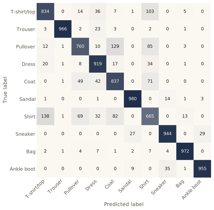
Read the matrix row by row. Trousers (row 2) and bags (row 9) are almost always right. The worst row is Shirt: only 665 of 1,000 shirts were predicted correctly, and 138 of them were called T-shirt/top. Going the other way, 103 T-shirts were called shirts, and 129 pullovers were called coats. Among the shoes, sneakers, sandals, and ankle boots are sometimes swapped for one another.
Every large mistake is between classes that look alike, and at 28 × 28 pixels even a person would hesitate over some of them. So part of the remaining error is in the data, not the model: the labels are sometimes ambiguous at this resolution. A confusion matrix tells you where to look — for example, by plotting the shirts that were predicted as T-shirts and deciding whether the model or the label is wrong. That is more useful than any single accuracy number.
Saving and loading the best model
Save the CNN’s learned weights the same way as in module 01, with state_dict():
from pathlib import Path

MODEL_PATH = Path("models")
MODEL_PATH.mkdir(parents=True, exist_ok=True)

MODEL_NAME = "03_pytorch_computer_vision_model_2.pth"
MODEL_SAVE_PATH = MODEL_PATH / MODEL_NAME

print(f"Saving model to: {MODEL_SAVE_PATH}")
torch.save(obj=model_2.state_dict(), f=MODEL_SAVE_PATH)
Saving model to: models/03_pytorch_computer_vision_model_2.pth
To load it, create a fresh instance of the same class with the same hyperparameters — the saved file holds only the numbers, not the architecture — then load the weights into it:
loaded_model_2 = FashionMNISTModelV2(input_shape=1, hidden_units=10,
                                     output_shape=len(class_names))
loaded_model_2.load_state_dict(torch.load(f=MODEL_SAVE_PATH))
loaded_model_2 = loaded_model_2.to(device)

loaded_model_2_results = eval_model(model=loaded_model_2,
                                    data_loader=test_dataloader,
                                    loss_fn=loss_fn, accuracy_fn=accuracy_fn,
                                    device=device)
loaded_model_2_results
{'model_name': 'FashionMNISTModelV2', 'model_loss': 0.31716408889990644, 'model_acc': 88.33865814696486}
Check that the loaded model gives the same results as the original. Tiny differences in the last decimal places can come from floating-point arithmetic, so compare with a tolerance rather than exact equality:
torch.isclose(torch.tensor(model_2_results["model_loss"]),
              torch.tensor(loaded_model_2_results["model_loss"]),
              atol=1e-08, rtol=1e-4)
tensor(True)
Watch out. If you change
hidden_unitswhen you create the new instance,load_state_dictfails with a “size mismatch” error: the saved weights no longer fit the layers. Keep a note of the hyperparameters next to every saved model — module 07 shows how to do this systematically.
Summary
| Task | Code |
|---|---|
| Load a torchvision dataset | datasets.FashionMNIST(root="data", train=True, download=True, transform=ToTensor()) |
| Image tensor shapes | one image [C, H, W]; a batch [N, C, H, W] |
| Make mini-batches | DataLoader(dataset, batch_size=32, shuffle=True) |
| Flatten images for linear layers | nn.Flatten() |
| Convolution | nn.Conv2d(in_channels, out_channels, kernel_size, stride, padding) |
| Pooling | nn.MaxPool2d(kernel_size=2) halves height and width |
| Output size of a conv layer | \(\lfloor (H + 2P - K)/S \rfloor + 1\) |
Find a classifier’s in_features |
pass a dummy input through the layers and print the shapes |
| Train and evaluate | train_step(...), test_step(...), eval_model(...) |
| Compare models | pd.DataFrame([results_0, results_1, results_2]) |
| Confusion matrix | sklearn.metrics.confusion_matrix, ConfusionMatrixDisplay |
| Save and load | torch.save(model.state_dict(), path), model.load_state_dict(torch.load(path)) |
Three ideas to carry forward: images are batched [N, C, H, W] tensors, and most bugs are a mismatch in that shape; convolutional layers work because they look at neighboring pixels together, with kernels that are learned rather than designed; and a model is only better than another if a fair comparison — same data, same measures, plus the cost in time — says so.
Exercises
- Name three places in industry, ideally in your own field, where computer vision is used. For each, say whether it is classification, detection, or segmentation.
- Load
torchvision.datasets.MNIST(handwritten digits) instead of FashionMNIST. Plot at least five training samples with their labels, and turn both splits intoDataLoaders withbatch_size=32. - Train
FashionMNISTModelV2(TinyVGG) on MNIST for three epochs. How does its test accuracy compare with FashionMNIST, and why might digits be easier than clothing? - Create a random tensor of shape
[1, 3, 64, 64]and pass it throughnn.Conv2dlayers withkernel_size1, 3, 5, and 7 (stride 1, no padding). Predict each output shape with the formula before you run the code. - Change
model_2to take 64 × 64 images: what mustin_featuresbecome? Confirm with a dummy input. - Remove the final
nn.ReLU()fromFashionMNISTModelV1and retrain for three epochs. Does the accuracy change? Explain what that last ReLU was doing to the logits. - Plot ten test images that model 2 got wrong, with the predicted and true label for each. Would you call these modeling errors, or are some of the labels themselves ambiguous?
- If you have a Colab GPU, train model 0 and model 2 on both CPU and GPU and record the times. Which model benefits more from the GPU?
- In your own words. Pick an inspection or measurement task from your engineering field that uses images. Describe the input tensor shape, the classes (or other outputs) you would want, and one pair of classes you expect a model to confuse — and why.
Going further
- CNN Explainer — an interactive TinyVGG in the browser. Upload your own image and watch each feature map. Twenty minutes here is well spent.
torch.nn.Conv2dandtorch.nn.MaxPool2ddocumentation, including the exact output-size formulas with dilation.- A guide to convolution arithmetic for deep learning (Dumoulin and Visin) — clear diagrams of stride and padding.
- The torchvision datasets and models catalogs — browse what is available for classification, detection, and segmentation.
- Stanford CS231n notes on convolutional networks — the standard deeper treatment.
These notes follow the path of Daniel Bourke's Learn PyTorch for Deep Learning (MIT license), rewritten for engineering students meeting Python and machine learning for the first time.