EAS 510 · Module 04 · Week 5
Custom Datasets
Bringing your own images — folder layouts, transforms, data augmentation, and diagnosing over- and underfitting.
Companion reading: Learn PyTorch for Deep Learning, chapter 04
By the end of this module you can
- Organize your own images in the standard train/test/class folder layout and explore it with a few lines of Python.
- Open an image with PIL, turn it into a tensor with
transforms, and plot it before and after. - Load a folder of images with
ImageFolder, and write your ownDatasetsubclass that does the same job. - Explain data augmentation and apply
TrivialAugmentWideto training images only. - Train TinyVGG with reusable
train_step,test_step, andtrainfunctions, and plot its loss curves. - Diagnose underfitting and overfitting from loss curves and choose remedies for each.
- Predict the class of a new image downloaded from the internet, fixing its datatype, shape, and device first.
Contents
- What a custom dataset is
- Getting the data
- Becoming one with the data
- Transforming data
- Option 1: loading images with ImageFolder
- Option 2: writing your own Dataset
- Data augmentation
- Model 0: TinyVGG without augmentation
- Reading loss curves
- Model 1: TinyVGG with data augmentation
- Comparing the two models
- Predicting on your own image
- Where datasets come from, and who is in them
- Summary
- Exercises
- Going further
In module 03 the data arrived ready to use: one line of torchvision.datasets gave us 70,000 labeled, same-sized images. Real projects do not start that way. Your data is a folder of photos from a site inspection, a set of micrographs from the lab, or a directory of camera frames from a production line — different sizes, different file names, and no PyTorch code that knows about them.
This module is about that step: getting your own images into a form a model can learn from. We use a small food dataset — photos of pizza, steak, and sushi — because it looks like a real custom dataset: a few hundred pictures of varying size, sorted into folders. We load it two ways (with a ready-made class, and with one we write ourselves), train two versions of TinyVGG from module 03, and use their loss curves to diagnose what goes wrong. That diagnosis — underfitting or overfitting, and what to do about each — is one of the most useful skills in the course.
What a custom dataset is
A custom dataset is any collection of data specific to your problem that is not already packaged for PyTorch. Whatever the data, the goal is the same: write a Dataset that returns one (input, label) pair at a time, then wrap it in a DataLoader for batching — exactly the two pieces you used in module 03.
PyTorch has a companion library for each kind of data, and each one provides datasets, transforms, and helper functions in the same pattern:
| Kind of data | Library | Example problem |
|---|---|---|
| Images | torchvision |
Is this photo of a weld good or defective? |
| Audio | torchaudio |
Does this bearing sound like it is failing? |
| Text | torchtext |
Is this maintenance report about corrosion or wear? |
| Recommendations | TorchRec |
Which spare parts should this customer see? |
(torchtext is no longer developed; for text, the Hugging Face libraries are now the usual choice.) Our data is images, so we use torchvision.
import torch
from torch import nn

device = "cuda" if torch.cuda.is_available() else "cpu"
torch.__version__, device
('2.14.0+cu130', 'cpu')
Getting the data
Our images come from Food-101, a public dataset of 101,000 photos in 101 food categories (750 training and 250 test images per category). We use a small subset: three classes — pizza, steak, and sushi — and about 10% of their images, roughly 75 training and 25 test images per class.
Starting small is deliberate. While you are writing and debugging code, you want each experiment to finish in seconds, not hours. Once the pipeline works, you scale up.
The subset lives as a zip file in the GitHub repository of Learn PyTorch for Deep Learning, the book these notes follow. This cell downloads and unzips it, and skips the download if the folder already exists:
import requests
import zipfile
from pathlib import Path

data_path = Path("data/")
image_path = data_path / "pizza_steak_sushi"

if image_path.is_dir():
    print(f"{image_path} already exists, skipping download.")
else:
    print(f"Creating {image_path} ...")
    image_path.mkdir(parents=True, exist_ok=True)

    url = ("https://raw.githubusercontent.com/mrdbourke/pytorch-deep-learning/"
           "main/data/pizza_steak_sushi.zip")
    with open(data_path / "pizza_steak_sushi.zip", "wb") as f:
        print("Downloading pizza, steak, sushi data ...")
        f.write(requests.get(url).content)

    with zipfile.ZipFile(data_path / "pizza_steak_sushi.zip", "r") as zip_ref:
        print("Unzipping pizza, steak, sushi data ...")
        zip_ref.extractall(image_path)
Creating data/pizza_steak_sushi ...
Downloading pizza, steak, sushi data ...
Unzipping pizza, steak, sushi data ...
Path (from Python’s pathlib) represents a file or folder location. Joining paths with /, as in data_path / "pizza_steak_sushi", works on every operating system.
Becoming one with the data
Before writing any model code, spend time with the data: how is it organized, how much is there, what does it look like? Most failed projects fail here, not in the model.
The standard folder layout
Image classification data is very often stored like this: one folder for training, one for testing, and inside each, one folder per class, named after the class. The left column of the figure below shows it for our data; test/ repeats the layout of train/.
The folder name is the label. No spreadsheet of labels is needed: a photo of steak is labeled “steak” because it sits in the steak folder. If you are collecting your own images, sorting them into this layout is the easiest way to make them usable by standard tools.
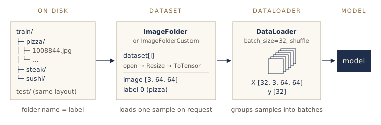
Dataset knows how to load and transform one image and find its label from the folder name; the DataLoader groups many of them into shuffled batches.A short function walks through the folders and counts what is in each:
import os

def walk_through_dir(dir_path):
    """Print how many folders and images are in dir_path and below it."""
    for dirpath, dirnames, filenames in sorted(os.walk(dir_path)):
        print(f"{len(dirnames)} directories and {len(filenames)} images "
              f"in '{dirpath}'")

walk_through_dir(image_path)
2 directories and 0 images in 'data/pizza_steak_sushi'
3 directories and 0 images in 'data/pizza_steak_sushi/test'
0 directories and 25 images in 'data/pizza_steak_sushi/test/pizza'
0 directories and 19 images in 'data/pizza_steak_sushi/test/steak'
0 directories and 31 images in 'data/pizza_steak_sushi/test/sushi'
3 directories and 0 images in 'data/pizza_steak_sushi/train'
0 directories and 78 images in 'data/pizza_steak_sushi/train/pizza'
0 directories and 75 images in 'data/pizza_steak_sushi/train/steak'
0 directories and 72 images in 'data/pizza_steak_sushi/train/sushi'
225 training and 75 test images in all, close to 75 and 25 per class. The training classes are nearly balanced — about the same number of each — which makes accuracy easy to interpret: a model that always answered “pizza” would score only about one in three. (The test split is less even, 19 steak against 31 sushi; worth knowing when you read the results.) Store the two top-level paths:
train_dir = image_path / "train"
test_dir = image_path / "test"
train_dir, test_dir
(PosixPath('data/pizza_steak_sushi/train'), PosixPath('data/pizza_steak_sushi/test'))
Looking at an image
To open an image file we use PIL (the Python Imaging Library, installed as Pillow), the standard Python library for reading and writing image files. Pick a random image, get its class from the name of the folder it sits in, and print its size:
import random
from PIL import Image

random.seed(42)

image_path_list = list(image_path.glob("*/*/*.jpg"))   # every .jpg two folders down
random_image_path = random.choice(image_path_list)
image_class = random_image_path.parent.stem            # folder name = label

img = Image.open(random_image_path)

print(f"Number of images: {len(image_path_list)}")
print(f"Random image path: {random_image_path}")
print(f"Image class: {image_class}")
print(f"Image height: {img.height}")
print(f"Image width: {img.width}")
Number of images: 300
Random image path: data/pizza_steak_sushi/test/pizza/2003290.jpg
Image class: pizza
Image height: 384
Image width: 512
glob("*/*/*.jpg") means “any folder, then any folder, then any file ending in .jpg”, which matches train/pizza/xxx.jpg and the like. To plot the image with matplotlib, turn it into a NumPy array first:
import numpy as np
import matplotlib.pyplot as plt

img_as_array = np.asarray(img)

plt.figure(figsize=(8, 6))
plt.imshow(img_as_array)
plt.title(f"{image_class} | shape {img_as_array.shape} -> [H, W, C]")
plt.axis(False);

img_as_array.shape, img_as_array.dtype
((384, 512, 3), dtype('uint8'))
Notice two things. The array is channels last — [height, width, color_channels] — while PyTorch layers want channels first. And its datatype is uint8: whole numbers from 0 to 255, where PyTorch models want float32 values. Both have to be fixed before a model can see the image. Also, the images do not all have the same size; a batch needs them to.
Transforming data
A transform is a function applied to each image as it is loaded. torchvision.transforms has dozens; we need three, chained together with transforms.Compose:
Resize((64, 64))— make every image 64 × 64 pixels. Small images train fast; module 06 uses larger ones.RandomHorizontalFlip(p=0.5)— mirror the image left-to-right half of the time. (More on why in the section on data augmentation.)ToTensor()— convert to afloat32tensor, channels first, with values scaled from 0–255 down to 0–1.
from torch.utils.data import DataLoader
from torchvision import datasets, transforms

data_transform = transforms.Compose([
    transforms.Resize(size=(64, 64)),
    transforms.RandomHorizontalFlip(p=0.5),
    transforms.ToTensor(),
])

transformed = data_transform(img)
print(f"Shape: {transformed.shape}  dtype: {transformed.dtype}")
print(f"Values from {transformed.min():.3f} to {transformed.max():.3f}")
Shape: torch.Size([3, 64, 64])  dtype: torch.float32
Values from 0.000 to 0.914
All three problems from the last section are solved: channels first, float32 between 0 and 1, and a fixed size. It is worth looking at the result, to make sure a transform does what you think. This function plots a few original images next to their transformed versions:
def plot_transformed_images(image_paths, transform, n=3, seed=42):
    """Plot n random images from image_paths, before and after transform."""
    random.seed(seed)
    random_image_paths = random.sample(image_paths, k=n)
    for image_path in random_image_paths:
        with Image.open(image_path) as f:
            fig, ax = plt.subplots(1, 2)
            ax[0].imshow(f)
            ax[0].set_title(f"Original\nSize: {f.size}")
            ax[0].axis("off")

            # [C, H, W] -> [H, W, C] for matplotlib
            transformed_image = transform(f).permute(1, 2, 0)
            ax[1].imshow(transformed_image)
            ax[1].set_title(f"Transformed\nSize: {transformed_image.shape}")
            ax[1].axis("off")

            fig.suptitle(f"Class: {image_path.parent.stem}", fontsize=16)

plot_transformed_images(image_path_list, transform=data_transform, n=3)
In the plots you will see the resized images look blurrier — at 64 × 64 a lot of detail is gone. That is a tradeoff: smaller images mean faster training but less information for the model.
Option 1: loading images with ImageFolder
Because the standard folder layout is so common, torchvision has a ready-made Dataset for it: datasets.ImageFolder. Point it at a folder, give it a transform, and it finds every image and labels it by its folder name.
train_data = datasets.ImageFolder(root=train_dir,
                                  transform=data_transform,  # for each image
                                  target_transform=None)     # for labels (none)

# No random flip for the test images
test_transform = transforms.Compose([transforms.Resize((64, 64)),
                                     transforms.ToTensor()])
test_data = datasets.ImageFolder(root=test_dir, transform=test_transform)

print(f"Train data:\n{train_data}\nTest data:\n{test_data}")
Train data:
Dataset ImageFolder
    Number of datapoints: 225
    Root location: data/pizza_steak_sushi/train
    StandardTransform
Transform: Compose(
               Resize(size=(64, 64), interpolation=bilinear, max_size=None, antialias=True)
               RandomHorizontalFlip(p=0.5)
               ToTensor()
           )
Test data:
Dataset ImageFolder
    Number of datapoints: 75
    Root location: data/pizza_steak_sushi/test
    StandardTransform
Transform: Compose(
               Resize(size=(64, 64), interpolation=bilinear, max_size=None, antialias=True)
               ToTensor()
           )
The class names and their label numbers come from the folder names, in alphabetical order:
class_names = train_data.classes
class_dict = train_data.class_to_idx
print(class_names)
print(class_dict)
print(f"{len(train_data)} training images, {len(test_data)} test images")
['pizza', 'steak', 'sushi']
{'pizza': 0, 'steak': 1, 'sushi': 2}
225 training images, 75 test images
Indexing gives an (image, label) pair, already transformed:
img, label = train_data[0]
print(f"Image tensor shape: {img.shape}  dtype: {img.dtype}")
print(f"Label: {label} ({class_names[label]})")
Image tensor shape: torch.Size([3, 64, 64])  dtype: torch.float32
Label: 0 (pizza)
To plot a tensor image, permute it back to channels last: plt.imshow(img.permute(1, 2, 0)).
DataLoaders
As in module 03, wrap the datasets in DataLoaders. One new argument is num_workers: how many separate processes load and transform images in the background while the model trains. With FashionMNIST the images were tiny and already in memory; here each batch means opening, decoding, and resizing JPEG files, so parallel loading helps. os.cpu_count() uses one worker per CPU core.
We start with batch_size=1 just to check the shapes; we will use 32 for training.
train_dataloader = DataLoader(dataset=train_data, batch_size=1,
                              num_workers=os.cpu_count(), shuffle=True)
test_dataloader = DataLoader(dataset=test_data, batch_size=1,
                             num_workers=os.cpu_count(), shuffle=False)

img, label = next(iter(train_dataloader))
print(f"Image shape: {img.shape} -> [batch_size, color_channels, height, width]")
print(f"Label shape: {label.shape}")
Image shape: torch.Size([1, 3, 64, 64]) -> [batch_size, color_channels, height, width]
Label shape: torch.Size([1])
Watch out. On Windows and macOS,
num_workersgreater than 0 can fail or hang when you run a plain.pyscript (not a notebook) unless the training code sits underif __name__ == "__main__":. If loading hangs, setnum_workers=0to rule this out.
Option 2: writing your own Dataset
ImageFolder covers the standard layout. But what if your labels are in a spreadsheet rather than folder names, your images are TIFF stacks from a microscope, or each sample is an image plus a sensor reading? No ready-made class fits, and you write your own. To see how, we rebuild ImageFolder from scratch; the same recipe works for any data.
Ready-made (ImageFolder) |
Your own Dataset |
|
|---|---|---|
| Effort | One line | More code to write and test |
| Flexibility | Only the standard layout | Any file format, any label source |
| Risk | Well tested | Bugs are yours to find |
A custom dataset is a Python class that inherits from torch.utils.data.Dataset — it starts as a copy of PyTorch’s general Dataset and fills in the specifics. PyTorch requires two methods:
__len__— return how many samples there are (this is whatlen(dataset)calls);__getitem__— given an index, return one(sample, label)pair (this is whatdataset[i]calls).
A helper to find the classes
First, a function that produces the same classes list and class_to_idx dictionary as ImageFolder, from the folder names:
from typing import Tuple, Dict, List

def find_classes(directory: str) -> Tuple[List[str], Dict[str, int]]:
    """Find the class folder names in directory and map each to an index."""
    # 1. Scan the directory for folder names, sorted alphabetically
    classes = sorted(e.name for e in os.scandir(directory) if e.is_dir())
    # 2. Raise an error if there are none
    if not classes:
        raise FileNotFoundError(f"Couldn't find any classes in {directory}.")
    # 3. Map each class name to an index: {'pizza': 0, 'steak': 1, ...}
    class_to_idx = {cls_name: i for i, cls_name in enumerate(classes)}
    return classes, class_to_idx

find_classes(train_dir)
(['pizza', 'steak', 'sushi'], {'pizza': 0, 'steak': 1, 'sushi': 2})
Identical to ImageFolder’s.
ImageFolderCustom
Now the dataset itself. __init__ runs once when the dataset is created: it collects every image path and the class names. __getitem__ runs every time a sample is requested: it opens that one image, transforms it, and looks up its label. Images are opened only when needed, so the dataset never has to hold every image in memory at once.
from torch.utils.data import Dataset

class ImageFolderCustom(Dataset):
    def __init__(self, targ_dir: str, transform=None) -> None:
        # All image paths (assumes .jpg files two levels down: class/image.jpg)
        self.paths = list(Path(targ_dir).glob("*/*.jpg"))
        self.transform = transform
        self.classes, self.class_to_idx = find_classes(targ_dir)

    def load_image(self, index: int) -> Image.Image:
        "Open the image at position index."
        return Image.open(self.paths[index])

    def __len__(self) -> int:
        "Number of samples."
        return len(self.paths)

    def __getitem__(self, index: int) -> Tuple[torch.Tensor, int]:
        "Return one sample: (transformed image, class index)."
        img = self.load_image(index)
        class_name = self.paths[index].parent.name     # folder name, e.g. "pizza"
        class_idx = self.class_to_idx[class_name]
        if self.transform:
            return self.transform(img), class_idx
        return img, class_idx
Try it with the same kind of transforms (a random flip for training, none for testing):
train_transforms = transforms.Compose([
    transforms.Resize((64, 64)),
    transforms.RandomHorizontalFlip(p=0.5),
    transforms.ToTensor(),
])
test_transforms = transforms.Compose([
    transforms.Resize((64, 64)),
    transforms.ToTensor(),
])

train_data_custom = ImageFolderCustom(train_dir, transform=train_transforms)
test_data_custom = ImageFolderCustom(test_dir, transform=test_transforms)

print(f"Lengths: {len(train_data_custom)}, {len(test_data_custom)}")
print(f"Classes: {train_data_custom.classes}")
same_lengths = (len(train_data_custom) == len(train_data)
                and len(test_data_custom) == len(test_data))
print(f"Same lengths as ImageFolder: {same_lengths}")
same_classes = train_data_custom.classes == train_data.classes
print(f"Same classes as ImageFolder: {same_classes}")
Lengths: 225, 75
Classes: ['pizza', 'steak', 'sushi']
Same lengths as ImageFolder: True
Same classes as ImageFolder: True
Our class behaves like the ready-made one. It also plugs into a DataLoader without any changes, because a DataLoader only ever calls __len__ and __getitem__. For a quick one-image check we load in the main process (num_workers=0), which also makes any error in __getitem__ easier to read:
train_dataloader_custom = DataLoader(dataset=train_data_custom, batch_size=1,
                                     num_workers=0, shuffle=True)

img_custom, label_custom = next(iter(train_dataloader_custom))
print(f"Image shape: {img_custom.shape} -> [batch_size, channels, height, width]")
print(f"Label shape: {label_custom.shape}")
Image shape: torch.Size([1, 3, 64, 64]) -> [batch_size, channels, height, width]
Label shape: torch.Size([1])
Same shapes as with ImageFolder. Whatever your data looks like, this is the pattern to follow: collect the list of samples in __init__, load and transform one sample in __getitem__.
Note. For spot checks, write a small function that plots a handful of random samples from any
Dataset— pick indices withrandom.sample(range(len(dataset)), k=5), thenplt.imshow(image.permute(1, 2, 0))for each. Looking at what theDatasetactually returns (not what the files contain) catches wrong labels and broken transforms early.
Data augmentation
Our training set has 75 photos of each food. A model can simply memorize them — this pizza has a basil leaf in the top left, so it is pizza — without learning what makes pizza pizza. One cheap way to fight that is data augmentation: apply random changes to each training image every time it is loaded, so the model never sees exactly the same picture twice. Flipping, rotating, cropping, shifting brightness and contrast — each changed image is still obviously a pizza, and the model is pushed to learn features that survive those changes.
The random horizontal flip we have been using is one augmentation. Choosing the right mix by hand is fiddly, so recent research has looked for simple automatic recipes. torchvision’s TrivialAugmentWide is one: for each image, it picks one augmentation at random from a list (rotation, shear, color, contrast, sharpness, and others) and applies it at a random strength. num_magnitude_bins sets how many strength levels there are to choose from, spread between barely visible and strong; 31 is the default.
train_transform_trivial_augment = transforms.Compose([
    transforms.Resize((64, 64)),
    transforms.TrivialAugmentWide(num_magnitude_bins=31),
    transforms.ToTensor(),
])

# Never augment test images: we want to measure the model on real data
test_transform = transforms.Compose([
    transforms.Resize((64, 64)),
    transforms.ToTensor(),
])

plot_transformed_images(image_paths=image_path_list,
                        transform=train_transform_trivial_augment, n=3)
Run the plotting cell several times: the same image comes out differently each time — rotated, recolored, sheared, or sometimes unchanged.
Watch out. Augment only the training data. The test set is there to estimate how the model does on real images; changing them would make that estimate meaningless.
Augmentation creates no new information, so it is not as good as more real data. But it is free, and with small datasets it often helps. Whether it helps here is an experiment we are about to run.
Model 0: TinyVGG without augmentation
We will train two models that differ in exactly one thing — augmentation — so any difference in results comes from it. Model 0 uses the plain transform.
Data
simple_transform = transforms.Compose([
    transforms.Resize((64, 64)),
    transforms.ToTensor(),
])

train_data_simple = datasets.ImageFolder(root=train_dir, transform=simple_transform)
test_data_simple = datasets.ImageFolder(root=test_dir, transform=simple_transform)

BATCH_SIZE = 32
NUM_WORKERS = os.cpu_count()

train_dataloader_simple = DataLoader(train_data_simple, batch_size=BATCH_SIZE,
                                     shuffle=True, num_workers=NUM_WORKERS)
test_dataloader_simple = DataLoader(test_data_simple, batch_size=BATCH_SIZE,
                                    shuffle=False, num_workers=NUM_WORKERS)

print(f"Batch size {BATCH_SIZE}, {NUM_WORKERS} workers")
print(f"{len(train_dataloader_simple)} train batches, "
      f"{len(test_dataloader_simple)} test batches")
Batch size 32, 2 workers
8 train batches, 3 test batches
225 training images in batches of 32 gives 8 batches (the last one has only 1 image).
The TinyVGG class
This is the TinyVGG from module 03, now as a general class called TinyVGG. Two differences: the input has 3 color channels, and the convolutions use padding=0, so each one shrinks the image by 2 pixels. Trace a 64 × 64 image through it:
- block 1: 64 → 62 → 60 (two convolutions), then max pool → 30;
- block 2: 30 → 28 → 26, then max pool → 13.
So the classifier receives hidden_units × 13 × 13 numbers.
class TinyVGG(nn.Module):
    """TinyVGG from the CNN Explainer website.
    See https://poloclub.github.io/cnn-explainer/"""
    def __init__(self, input_shape: int, hidden_units: int, output_shape: int):
        super().__init__()
        self.conv_block_1 = nn.Sequential(
            nn.Conv2d(in_channels=input_shape, out_channels=hidden_units,
                      kernel_size=3, stride=1, padding=0),
            nn.ReLU(),
            nn.Conv2d(in_channels=hidden_units, out_channels=hidden_units,
                      kernel_size=3, stride=1, padding=0),
            nn.ReLU(),
            nn.MaxPool2d(kernel_size=2, stride=2),
        )
        self.conv_block_2 = nn.Sequential(
            nn.Conv2d(hidden_units, hidden_units, kernel_size=3, padding=0),
            nn.ReLU(),
            nn.Conv2d(hidden_units, hidden_units, kernel_size=3, padding=0),
            nn.ReLU(),
            nn.MaxPool2d(2),
        )
        self.classifier = nn.Sequential(
            nn.Flatten(),
            nn.Linear(in_features=hidden_units * 13 * 13,  # 64x64 in -> 13x13
                      out_features=output_shape),
        )

    def forward(self, x: torch.Tensor):
        return self.classifier(self.conv_block_2(self.conv_block_1(x)))

torch.manual_seed(42)
model_0 = TinyVGG(input_shape=3,                    # color channels (RGB)
                  hidden_units=10,
                  output_shape=len(train_data.classes)).to(device)
model_0
TinyVGG(
  (conv_block_1): Sequential(
    (0): Conv2d(3, 10, kernel_size=(3, 3), stride=(1, 1))
    (1): ReLU()
    (2): Conv2d(10, 10, kernel_size=(3, 3), stride=(1, 1))
    (3): ReLU()
    (4): MaxPool2d(kernel_size=2, stride=2, padding=0, dilation=1, ceil_mode=False)
  )
  (conv_block_2): Sequential(
    (0): Conv2d(10, 10, kernel_size=(3, 3), stride=(1, 1))
    (1): ReLU()
    (2): Conv2d(10, 10, kernel_size=(3, 3), stride=(1, 1))
    (3): ReLU()
    (4): MaxPool2d(kernel_size=2, stride=2, padding=0, dilation=1, ceil_mode=False)
  )
  (classifier): Sequential(
    (0): Flatten(start_dim=1, end_dim=-1)
    (1): Linear(in_features=1690, out_features=3, bias=True)
  )
)
A forward pass on one image
Before training anything, check that one image goes through without a shape error. It is the cheapest test there is:
img_batch, label_batch = next(iter(train_dataloader_simple))
img_single, label_single = img_batch[0].unsqueeze(dim=0), label_batch[0]
print(f"Single image shape: {img_single.shape}\n")

model_0.eval()
with torch.inference_mode():
    pred = model_0(img_single.to(device))

print(f"Output logits:\n{pred}\n")
print(f"Output prediction probabilities:\n{torch.softmax(pred, dim=1)}\n")
print(f"Output prediction label: {torch.argmax(torch.softmax(pred, dim=1), dim=1)}")
print(f"Actual label: {label_single}")
Single image shape: torch.Size([1, 3, 64, 64])

Output logits:
tensor([[ 0.0208, -0.0020,  0.0095]])

Output prediction probabilities:
tensor([[0.3371, 0.3295, 0.3333]])

Output prediction label: tensor([0])
Actual label: 0
The untrained model gives each class roughly a one-in-three probability: it is guessing, as it should be before training.
Checking shapes with torchinfo
Tracing shapes by hand gets tedious for bigger models. The torchinfo package does it for you: give it the model and an input size, and it prints each layer’s output shape and parameter count. (In Colab, install it first with pip install torchinfo.)
!pip install -q torchinfo
from torchinfo import summary

# verbose=0: return the table without also printing it
summary(model_0, input_size=[1, 3, 64, 64], verbose=0)
==========================================================================================
Layer (type:depth-idx)                   Output Shape              Param #
==========================================================================================
TinyVGG                                  [1, 3]                    --
├─Sequential: 1-1                        [1, 10, 30, 30]           --
│    └─Conv2d: 2-1                       [1, 10, 62, 62]           280
│    └─ReLU: 2-2                         [1, 10, 62, 62]           --
│    └─Conv2d: 2-3                       [1, 10, 60, 60]           910
│    └─ReLU: 2-4                         [1, 10, 60, 60]           --
│    └─MaxPool2d: 2-5                    [1, 10, 30, 30]           --
├─Sequential: 1-2                        [1, 10, 13, 13]           --
│    └─Conv2d: 2-6                       [1, 10, 28, 28]           910
│    └─ReLU: 2-7                         [1, 10, 28, 28]           --
│    └─Conv2d: 2-8                       [1, 10, 26, 26]           910
│    └─ReLU: 2-9                         [1, 10, 26, 26]           --
│    └─MaxPool2d: 2-10                   [1, 10, 13, 13]           --
├─Sequential: 1-3                        [1, 3]                    --
│    └─Flatten: 2-11                     [1, 1690]                 --
│    └─Linear: 2-12                      [1, 3]                    5,073
==========================================================================================
Total params: 8,083
Trainable params: 8,083
Non-trainable params: 0
Total mult-adds (Units.MEGABYTES): 5.69
==========================================================================================
Input size (MB): 0.05
Forward/backward pass size (MB): 0.71
Params size (MB): 0.03
Estimated Total Size (MB): 0.79
==========================================================================================
Read down the “Output Shape” column and you see the trace above: 62, 60, 30, 28, 26, 13, then 1,690 numbers after flattening, then 3 logits. The model has about eight thousand parameters, most of them in the final linear layer — tiny by modern standards. The “mult-adds” line counts the multiply-and-add operations for one image, in millions (about 5.7 million here), despite the odd unit label some torchinfo versions print.
Train and test functions that return results
In module 03, train_step and test_step printed their results. This time we want to plot how the loss changes from epoch to epoch, so they return the loss and accuracy instead, and a third function, train, runs them for several epochs and collects everything in a dictionary. Accuracy is now a fraction between 0 and 1 rather than a percentage.
def train_step(model: torch.nn.Module,
               dataloader: torch.utils.data.DataLoader,
               loss_fn: torch.nn.Module,
               optimizer: torch.optim.Optimizer,
               device: torch.device = device):
    """Train model for one epoch. Returns (loss, accuracy as a fraction)."""
    model.train()
    train_loss, train_acc = 0, 0
    for X, y in dataloader:
        X, y = X.to(device), y.to(device)
        y_pred = model(X)                         # 1. forward pass
        loss = loss_fn(y_pred, y)                 # 2. loss
        train_loss += loss.item()
        optimizer.zero_grad()                     # 3. zero the gradients
        loss.backward()                           # 4. backpropagation
        optimizer.step()                          # 5. update the weights
        y_pred_class = torch.argmax(torch.softmax(y_pred, dim=1), dim=1)
        train_acc += (y_pred_class == y).sum().item() / len(y_pred)
    return train_loss / len(dataloader), train_acc / len(dataloader)


def test_step(model: torch.nn.Module,
              dataloader: torch.utils.data.DataLoader,
              loss_fn: torch.nn.Module,
              device: torch.device = device):
    """Test model for one epoch. Returns (loss, accuracy as a fraction)."""
    model.eval()
    test_loss, test_acc = 0, 0
    with torch.inference_mode():
        for X, y in dataloader:
            X, y = X.to(device), y.to(device)
            test_pred_logits = model(X)
            test_loss += loss_fn(test_pred_logits, y).item()
            test_pred_labels = test_pred_logits.argmax(dim=1)
            test_acc += (test_pred_labels == y).sum().item() / len(test_pred_labels)
    return test_loss / len(dataloader), test_acc / len(dataloader)
def train(model: torch.nn.Module,
          train_dataloader: torch.utils.data.DataLoader,
          test_dataloader: torch.utils.data.DataLoader,
          optimizer: torch.optim.Optimizer,
          loss_fn: torch.nn.Module = nn.CrossEntropyLoss(),
          epochs: int = 5):
    """Train and test model for several epochs; return per-epoch results."""
    results = {"train_loss": [], "train_acc": [], "test_loss": [], "test_acc": []}

    for epoch in range(epochs):
        train_loss, train_acc = train_step(model=model, dataloader=train_dataloader,
                                           loss_fn=loss_fn, optimizer=optimizer)
        test_loss, test_acc = test_step(model=model, dataloader=test_dataloader,
                                        loss_fn=loss_fn)
        print(f"Epoch {epoch + 1} | train_loss: {train_loss:.4f} | "
              f"train_acc: {train_acc:.4f} | test_loss: {test_loss:.4f} | "
              f"test_acc: {test_acc:.4f}")

        results["train_loss"].append(train_loss)
        results["train_acc"].append(train_acc)
        results["test_loss"].append(test_loss)
        results["test_acc"].append(test_acc)

    return results
Training model 0
We use the Adam optimizer this time instead of SGD. Adam adapts the step size for each weight as training goes, and its default learning rate of 0.001 works well for many problems, which makes it a common first choice. Five epochs take well under a minute on this small dataset, even on a CPU.
torch.manual_seed(42)
torch.cuda.manual_seed(42)

NUM_EPOCHS = 5

model_0 = TinyVGG(input_shape=3, hidden_units=10,
                  output_shape=len(train_data.classes)).to(device)

loss_fn = nn.CrossEntropyLoss()
optimizer = torch.optim.Adam(params=model_0.parameters(), lr=0.001)

from timeit import default_timer as timer
start_time = timer()

model_0_results = train(model=model_0,
                        train_dataloader=train_dataloader_simple,
                        test_dataloader=test_dataloader_simple,
                        optimizer=optimizer,
                        loss_fn=loss_fn,
                        epochs=NUM_EPOCHS)

end_time = timer()
print(f"Total training time: {end_time - start_time:.1f} seconds")
Epoch 1 | train_loss: 1.1063 | train_acc: 0.3047 | test_loss: 1.0983 | test_acc: 0.3011
Epoch 2 | train_loss: 1.0998 | train_acc: 0.3281 | test_loss: 1.0697 | test_acc: 0.5417
Epoch 3 | train_loss: 1.0869 | train_acc: 0.4883 | test_loss: 1.0808 | test_acc: 0.4924
Epoch 4 | train_loss: 1.0844 | train_acc: 0.4023 | test_loss: 1.0607 | test_acc: 0.5833
Epoch 5 | train_loss: 1.0663 | train_acc: 0.4141 | test_loss: 1.0659 | test_acc: 0.5644
Total training time: 28.3 seconds
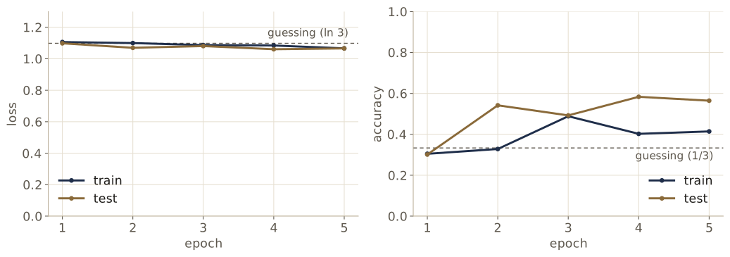
The results are poor. A useful reference point: a model that gives all three classes equal probability has a cross-entropy loss of \(\ln 3 \approx 1.099\). Our losses start there and fall only slightly in five epochs. Test accuracy wanders between about 30% and 58% — better than the 33% of guessing, but not by much — and the training accuracy is lower still. The model has barely learned anything, even about its own training data.
The accuracies also jump around from epoch to epoch. With only 8 training batches and 3 test batches, each reported number is an average of very few values, and with 75 test images a single image moves the test accuracy by more than a percentage point. Small datasets make noisy measurements; don’t read much into differences of a few percent.
Plotting loss curves
A table of numbers is hard to read. A loss curve — the loss plotted against the epoch, for training and test data — shows at a glance how training is going. This function draws loss and accuracy side by side from a results dictionary:
def plot_loss_curves(results: Dict[str, List[float]]):
    """Plot training and test loss and accuracy curves from a results dictionary."""
    loss, test_loss = results["train_loss"], results["test_loss"]
    accuracy, test_accuracy = results["train_acc"], results["test_acc"]
    epochs = range(1, len(loss) + 1)

    plt.figure(figsize=(15, 7))

    plt.subplot(1, 2, 1)
    plt.plot(epochs, loss, label="train_loss")
    plt.plot(epochs, test_loss, label="test_loss")
    plt.title("Loss")
    plt.xlabel("Epochs")
    plt.legend()

    plt.subplot(1, 2, 2)
    plt.plot(epochs, accuracy, label="train_accuracy")
    plt.plot(epochs, test_accuracy, label="test_accuracy")
    plt.title("Accuracy")
    plt.xlabel("Epochs")
    plt.legend();

plot_loss_curves(model_0_results)
Reading loss curves
The shape of the two curves tells you what kind of problem you have, and therefore what to try next.
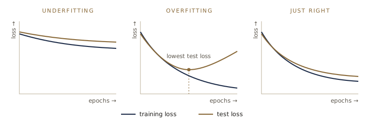
- Underfitting. Both losses stay high. The model has not learned the patterns in the data — even the training data. It is too simple, has not trained long enough, or cannot learn with its current settings.
- Overfitting. Training loss keeps falling, but test loss stops falling and starts to rise. The model is memorizing the training images, including their accidents (the basil leaf), instead of learning what generalizes to new ones.
- Just right. Both losses fall and level off close to each other. Test loss is usually a little higher than training loss; a small gap is normal.
In practice you move between the first two: first make the model powerful enough to fit the training data (fix underfitting), then rein it in until it generalizes (fix overfitting).
Remedies for overfitting
Techniques that reduce overfitting are collectively called regularization.
| Remedy | Why it helps |
|---|---|
| Get more data | More examples give the model more patterns to learn and fewer to memorize |
| Use data augmentation | Random changes make memorizing individual images harder, so the model has to learn features that generalize |
| Simplify the model | Fewer layers or hidden units give it less capacity to memorize |
| Use transfer learning | Start from a model that already learned general features on millions of images (module 06), so it needs fewer of yours |
| Add dropout | nn.Dropout randomly sets some of a layer’s outputs to zero during training, so the model cannot rely on any single one |
| Decay the learning rate | Take smaller steps as training goes on, so the model settles instead of chasing noise in individual batches |
| Stop early | Keep the weights from the epoch with the lowest validation loss and stop training when it starts to rise (see the note below on why that should not be the test set) |
Remedies for underfitting
| Remedy | Why it helps |
|---|---|
| Add layers or hidden units | More capacity to represent the patterns in the data |
| Train for longer | The model may simply not have had enough epochs |
| Tweak the learning rate | Too high and training bounces around without settling; too low and it barely moves |
| Use transfer learning | Pretrained features give a strong starting point, often solving underfitting and overfitting at once |
| Use less regularization | Too much augmentation or dropout can stop the model from fitting even the training data |
The two lists pull against each other: every remedy for one can push you toward the other. Transfer learning appears in both, which is one reason it is so widely used.
Note. We have been making decisions (how many epochs, which transform) by looking at the test set. In careful work you hold out a third split, the validation set, for those decisions, and touch the test set only once at the end; otherwise the test score is optimistic. With 25 images per class we skip this here, but keep it in mind for your projects.
Model 1: TinyVGG with data augmentation
Now the experiment: the same model, the same optimizer, the same number of epochs, and only the training transform changed to include TrivialAugmentWide.
train_data_augmented = datasets.ImageFolder(
    train_dir, transform=train_transform_trivial_augment)
test_data_simple = datasets.ImageFolder(test_dir, transform=test_transform)

torch.manual_seed(42)
train_dataloader_augmented = DataLoader(train_data_augmented, batch_size=BATCH_SIZE,
                                        shuffle=True, num_workers=NUM_WORKERS)
test_dataloader_simple = DataLoader(test_data_simple, batch_size=BATCH_SIZE,
                                    shuffle=False, num_workers=NUM_WORKERS)
torch.manual_seed(42)
torch.cuda.manual_seed(42)

model_1 = TinyVGG(input_shape=3, hidden_units=10,
                  output_shape=len(train_data_augmented.classes)).to(device)

loss_fn = nn.CrossEntropyLoss()
optimizer = torch.optim.Adam(params=model_1.parameters(), lr=0.001)

start_time = timer()
model_1_results = train(model=model_1,
                        train_dataloader=train_dataloader_augmented,
                        test_dataloader=test_dataloader_simple,
                        optimizer=optimizer,
                        loss_fn=loss_fn,
                        epochs=NUM_EPOCHS)
end_time = timer()
print(f"Total training time: {end_time - start_time:.1f} seconds")
Epoch 1 | train_loss: 1.1069 | train_acc: 0.3047 | test_loss: 1.0993 | test_acc: 0.2604
Epoch 2 | train_loss: 1.1019 | train_acc: 0.3203 | test_loss: 1.0719 | test_acc: 0.5417
Epoch 3 | train_loss: 1.0917 | train_acc: 0.4375 | test_loss: 1.0847 | test_acc: 0.4924
Epoch 4 | train_loss: 1.0914 | train_acc: 0.3164 | test_loss: 1.0678 | test_acc: 0.5833
Epoch 5 | train_loss: 1.0862 | train_acc: 0.3594 | test_loss: 1.0750 | test_acc: 0.5331
Total training time: 26.1 seconds
plot_loss_curves(model_1_results)
Model 1 did no better — if anything slightly worse. That is what the tables above predict. Augmentation is a remedy for overfitting: it makes the training task harder so the model cannot memorize. Our model was not memorizing; it was underfitting, and making its task harder does not help a model that cannot yet fit the easy version.
Comparing the two models
Turn each results dictionary into a pandas DataFrame (one row per epoch) and plot the two models against each other:
import pandas as pd

model_0_df = pd.DataFrame(model_0_results)
model_1_df = pd.DataFrame(model_1_results)
model_1_df.round(3)
   train_loss  train_acc  test_loss  test_acc
0       1.107      0.305      1.099     0.260
1       1.102      0.320      1.072     0.542
2       1.092      0.438      1.085     0.492
3       1.091      0.316      1.068     0.583
4       1.086      0.359      1.075     0.533
plt.figure(figsize=(15, 10))
epochs = range(1, len(model_0_df) + 1)

for i, metric in enumerate(["train_loss", "test_loss", "train_acc", "test_acc"]):
    plt.subplot(2, 2, i + 1)
    plt.plot(epochs, model_0_df[metric], label="Model 0 (no augmentation)")
    plt.plot(epochs, model_1_df[metric], label="Model 1 (TrivialAugment)")
    plt.title(metric)
    plt.xlabel("Epochs")
    plt.legend()
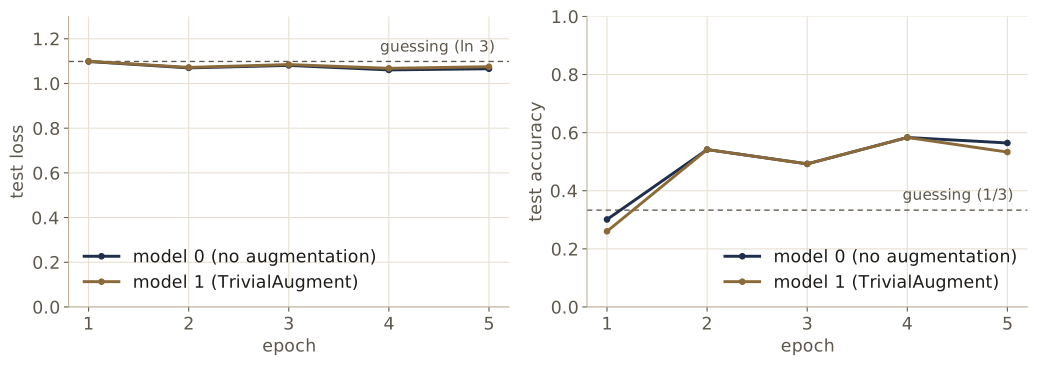
Neither model is good, and the difference between them is within the noise of a 75-image test set. The loss curves have told us what to do next: both models underfit, so the next experiments should come from the underfitting table — train for longer, add hidden units, get more data (a 20% subset is available), or use transfer learning. The exercises ask you to try the first three; module 06 does the fourth, which typically makes the biggest difference on a dataset this small.
Predicting on your own image
A model is only useful if it works on images it has never seen, taken by someone else. Let us try one: a photo of a pizza from the internet, not part of Food-101.
custom_image_path = data_path / "04-pizza-dad.jpeg"

url = ("https://raw.githubusercontent.com/mrdbourke/pytorch-deep-learning/"
       "main/images/04-pizza-dad.jpeg")

if not custom_image_path.is_file():
    with open(custom_image_path, "wb") as f:
        request = requests.get(url)
        print(f"Downloading {custom_image_path} ...")
        f.write(request.content)
else:
    print(f"{custom_image_path} already exists, skipping download.")
Downloading data/04-pizza-dad.jpeg ...
Loading the image as a tensor
torchvision.io.read_image reads an image file straight into a tensor:
import torchvision

custom_image_uint8 = torchvision.io.read_image(str(custom_image_path))

print(f"Custom image shape: {custom_image_uint8.shape}")
print(f"Custom image dtype: {custom_image_uint8.dtype}")
Custom image shape: torch.Size([3, 4032, 3024])
Custom image dtype: torch.uint8
It is channels first already, but it is much larger than 64 × 64, and its datatype is uint8 (0 to 255). Try it on the model as it is:
model_1.eval()
with torch.inference_mode():
    model_1(custom_image_uint8.to(device))
RuntimeError: Input type (unsigned char) and bias type (float) should be the same
A datatype error: the model’s weights are float32 and the image is uint8. This is the first of the three questions from module 00 — shape, datatype, device — and a new image will usually fail all three unless you prepare it the same way as the training data. Fix the datatype and scale the values to 0–1, as ToTensor did for our training images:
custom_image = torchvision.io.read_image(str(custom_image_path))
custom_image = custom_image.type(torch.float32) / 255.   # 0-255 -> 0-1

custom_image_transform = transforms.Compose([
    transforms.Resize((64, 64)),
])
custom_image_transformed = custom_image_transform(custom_image)

print(f"Original shape:    {custom_image.shape}")
print(f"Transformed shape: {custom_image_transformed.shape}")
Original shape:    torch.Size([3, 4032, 3024])
Transformed shape: torch.Size([3, 64, 64])
The last fix is the batch dimension: the model expects [batch_size, color_channels, height, width], so add one with unsqueeze(dim=0). Then move the image to the model’s device, predict, and turn the logits into a class:
model_1.eval()
with torch.inference_mode():
    custom_image_pred = model_1(
        custom_image_transformed.unsqueeze(dim=0).to(device))

custom_image_pred_probs = torch.softmax(custom_image_pred, dim=1)
custom_image_pred_label = torch.argmax(custom_image_pred_probs, dim=1).cpu()

print(f"Prediction logits:        {custom_image_pred}")
print(f"Prediction probabilities: {custom_image_pred_probs}")
print(f"Predicted class:          {class_names[custom_image_pred_label]}")
Prediction logits:        tensor([[-0.1154, -0.0205, -0.0051]])
Prediction probabilities: tensor([[0.3109, 0.3419, 0.3472]])
Predicted class:          sushi
The pipeline works: a photo of any size, from anywhere, goes in and a class comes out. The prediction itself is wrong — the photo shows a pizza — and the three probabilities are almost equal, which is the model’s way of saying it has no idea. That is what we should expect from a model with about 53% test accuracy.
A prediction function
Put those steps into one function that loads, prepares, predicts, and plots:
def pred_and_plot_image(model: torch.nn.Module,
                        image_path: str,
                        class_names: List[str] = None,
                        transform=None,
                        device: torch.device = device):
    """Predict the class of the image at image_path and plot it."""
    # 1. Load the image as float32 with values from 0 to 1
    target_image = torchvision.io.read_image(str(image_path))
    target_image = target_image.type(torch.float32) / 255.
    # 2. Apply the same transform as the training data (resize)
    if transform:
        target_image = transform(target_image)
    # 3. Predict with a batch dimension, on the model's device
    model.to(device)
    model.eval()
    with torch.inference_mode():
        target_image_pred = model(target_image.unsqueeze(dim=0).to(device))
    # 4. Logits -> probabilities -> label
    target_image_pred_probs = torch.softmax(target_image_pred, dim=1)
    target_image_pred_label = torch.argmax(target_image_pred_probs, dim=1)
    # 5. Plot the image (channels last) with the prediction and its probability
    plt.imshow(target_image.permute(1, 2, 0))
    pred_label = target_image_pred_label.cpu()
    prob = target_image_pred_probs.max().cpu()
    if class_names:
        title = f"Pred: {class_names[pred_label]} | Prob: {prob:.3f}"
    else:
        title = f"Pred: {pred_label} | Prob: {prob:.3f}"
    plt.title(title)
    plt.axis(False);

pred_and_plot_image(model=model_1, image_path=custom_image_path,
                    class_names=class_names,
                    transform=custom_image_transform, device=device)
The lesson generalizes beyond this example: a new input must go through the same preparation as the training data — same size, same datatype, same value range, same channel order — or the model’s predictions mean nothing. Many models that fail in use have not failed at all; they are being fed inputs prepared differently from the ones they were trained on.
Where datasets come from, and who is in them
Our three-food dataset came from Food-101, which was assembled from photos that users posted on a food-sharing website. Most datasets you will meet have a similar history: public benchmarks collected by research groups, often scraped from the web; data a company or lab collected for its own purposes; or data you collect yourself, with a camera on your own test rig. Before you use one, find out where it came from, how it was labeled, and under what license you may use it.
A model learns only what is in its training data, so who and what is in the data decides who and what the model works for. Food-101’s pizza photos are the pizzas that its contributors chose to photograph and post; a model trained on them may do worse on the kinds of pizza that rarely appeared there. That is a low-stakes example. The same mechanism has had serious consequences: the Gender Shades study (Buolamwini and Gebru, 2018) found that commercial face-analysis systems of the time made far more errors on darker-skinned women than on lighter-skinned men, and pointed out that the benchmark datasets used to evaluate such systems contained mostly lighter-skinned faces.
Engineering data has the same issue in a quieter form. A crack detector trained on photos of one bridge, taken on sunny days, may fail on another concrete mix, on a rainy day, or with a different camera. A defect classifier trained on one production line may not transfer to the line next door. Some habits that help:
- Document the data. Where, when, and how was it collected? By whom, with which equipment? Which cases are missing?
- Look at the class balance and the conditions, not just the labels: lighting, equipment, materials, locations, and, where people are involved, who they are.
- Test on data from where the model will be used, and report accuracy separately for important subgroups, not only on average. A 95% average can hide a group where the model is wrong half the time.
Note. A good test score shows only that the model works on data like the test set. If the test set was collected the same way as the training set, it shares the same gaps.
Summary
| Task | Code |
|---|---|
| Explore a folder of images | os.walk(path), Path(path).glob("*/*/*.jpg") |
| Open an image | PIL.Image.open(path), or torchvision.io.read_image(path) for a tensor |
| Prepare images | transforms.Compose([transforms.Resize((64, 64)), transforms.ToTensor()]) |
| Augment training images | transforms.TrivialAugmentWide(num_magnitude_bins=31), RandomHorizontalFlip() |
| Load the standard folder layout | datasets.ImageFolder(root=train_dir, transform=...) |
| Write your own dataset | subclass Dataset; implement __init__, __len__, __getitem__ |
| Batch it | DataLoader(dataset, batch_size=32, shuffle=True) |
| Inspect a model’s shapes | torchinfo.summary(model, input_size=[1, 3, 64, 64]) |
| Train and record results | results = train(model, train_dataloader, test_dataloader, optimizer, loss_fn, epochs) |
| Plot loss curves | plot_loss_curves(results) |
| Predict on a new image | read → float32 / 255 → resize → unsqueeze(0) → .to(device) → model |
Three ideas to carry forward: any data can be used with PyTorch once you can write a Dataset that returns one (input, label) pair; loss curves tell you whether to make the model stronger (underfitting) or to rein it in (overfitting); and a model is only as good, and as fair, as the data it was trained and tested on.
Exercises
- Our models are underfitting. List three things you could try to fix that, and for each, predict what it would do to the loss curves.
- Rebuild the data loading and TinyVGG model from this module in a fresh notebook, without looking back at the notes more than you need to.
- Train model 0 for 20 and then 50 epochs. Plot the loss curves each time. Does it start to overfit, and after how many epochs?
- Double the number of hidden units to 20 and train for 20 epochs. What happens to the results, and to the training time?
- Download the larger
pizza_steak_sushi_20_percent.zip(same URL, with_20_percentbefore.zip), which has twice as many images. Train model 0 on it for 20 epochs and compare with exercise 3. - Change
ImageFolderCustomso that it also accepts.pngand.jpegfiles. Test it on a folder where you have added a few of your own images. - Take your own photo of pizza, steak, or sushi (or find one online), and predict it with
pred_and_plot_image. Does the model get it right? Try a photo of something that is none of the three — what does the model say, and why can it not say “none of these”? - Write a
Datasetsubclass whose labels come from a CSV file with two columns,filenameandlabel, instead of from folder names. - In your own words. For an image-based task in your engineering field, describe how you would collect and organize the dataset, which conditions (equipment, lighting, material, site) it must cover, and one way the data could be biased so that the model fails in use.
Going further
- The PyTorch tutorial Datasets and DataLoaders, and Writing custom datasets, dataloaders and transforms.
- The torchvision transforms gallery — pictures of what each augmentation does.
- TrivialAugment: Tuning-free yet state-of-the-art data augmentation (Müller and Hutter, 2021), the paper behind
TrivialAugmentWide. - Datasheets for datasets (Gebru et al.) — a checklist of questions to answer about any dataset you build or use.
- Gender Shades (Buolamwini and Gebru, 2018) — the study on bias in face-analysis systems discussed above.
These notes follow the path of Daniel Bourke's Learn PyTorch for Deep Learning (MIT license), rewritten for engineering students meeting Python and machine learning for the first time.