EAS 510 · Module 05 · Week 6
Going Modular
Turning a notebook into a small Python package you can train from the command line and reuse in every later module.
Companion reading: Learn PyTorch for Deep Learning, chapter 05
By the end of this module you can
- Compare notebooks and Python scripts, and decide when a project should move from one to the other.
- Organize a training project into a small package of files —
data_setup.py,model_builder.py,engine.py,utils.py, andtrain.py— each with one job. - Write Python files from Colab with
%%writefileand run them with!python. - Read docstrings and type hints, and write both for a function of your own.
- Train a model with one command and change its hyperparameters with command-line flags built with
argparse. - Import the package into a notebook to load a saved model and evaluate it without copying any code.
Contents
- Notebooks and scripts
- What we are building
- Getting the data: get_data.py
- Datasets and DataLoaders: data_setup.py
- The model: model_builder.py
- Training and testing: engine.py
- Saving the model: utils.py
- Putting it together: train.py
- Reusing the package from a notebook
- Command-line arguments with argparse
- Summary
- Exercises
- Going further
In module 04 we built a complete image classifier for pizza, steak, and sushi photos: we downloaded the images, wrapped them in a Dataset and a DataLoader, defined TinyVGG, wrote train_step, test_step, and train, and saved the result. It worked — but it lived in one long notebook. To try a different model next week, you would have to scroll through dozens of cells, copy the ones you need, and hope you did not miss one.
This module adds no new machine learning. The data, the model, and the training loop are the ones you already know. What changes is where the code lives. We move each piece into its own Python file, collect the files in a folder called going_modular, and end up able to train the whole model with a single command:
python going_modular/train.py
Every later module in the course imports from this folder instead of redefining the same functions. Organizing code this way is called going modular, and it is how most PyTorch code outside of tutorials is written.
Notebooks and scripts
A notebook (Jupyter or Colab) is a document of cells that you run one at a time, with the output shown underneath each cell. A Python script is a plain text file ending in .py that runs from top to bottom in one go, usually from a command line — the text window, also called a terminal or shell, where you type commands instead of clicking.
What each is good at
| Notebooks | Python scripts | |
|---|---|---|
| Strengths | Fast to experiment: run one cell, look, change, rerun. Outputs, plots, and notes sit next to the code. Easy to share (a Colab link). | Easy to reuse: import a function into any other file. Work well with version control (Git), since each change is a readable line of text. Standard in open-source projects and on cloud and lab servers. |
| Weaknesses | Hard to reuse a piece without copying it. Hard to track changes over time. Cells can be run out of order, so the notebook’s state may not match what you see. | Less visual: no plot appears next to the code. You run the whole file, not one piece of it. |
When to move from notebook to scripts
The two are not rivals; they are stages. A common workflow, and the one we follow, is:
- Explore in a notebook. Load the data, look at it, try a model, plot the results.
- Once a piece works and you want it again, move it into a script. The data loading, the model class, and the training loop are good candidates — you will use all three in every experiment.
- Keep using notebooks for new experiments, but have them import the tested pieces instead of redefining them.
A useful rule of thumb: the second time you copy a cell into a new notebook, it belongs in a file.
This is not unlike the move from a hand calculation to a standard design procedure. The first time you size a beam you work it out on paper; by the tenth time, you have a spreadsheet template that you trust and reuse, and you save the scratch paper for the unusual cases.
How PyTorch code runs in the wild
Open almost any PyTorch project on GitHub and you will find a train.py that is started from the command line, with settings passed as flags — named options that begin with --:
python train.py --model tinyvgg --batch_size 32 --learning_rate 0.001 --num_epochs 10
Changing an experiment then means changing a flag, not editing code. We build exactly this by the end of the module.
What we are building
At the end of this module your Colab session will contain this folder layout:
going_modular/
├── get_data.py        downloads the images (run once)
├── data_setup.py      builds the DataLoaders
├── model_builder.py   defines TinyVGG
├── engine.py          train_step, test_step, train
├── utils.py           save_model
└── train.py           puts it all together
models/
└── 05_going_modular_script_mode_tinyvgg_model.pth
data/
└── pizza_steak_sushi/
    ├── train/  (pizza/, steak/, sushi/)
    └── test/   (pizza/, steak/, sushi/)
Each file maps onto a group of cells from the module 04 notebook.
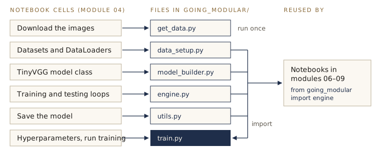
train.py contains almost no logic of its own: it imports the other four files and calls them in order. Later notebooks import the same files.A few terms. In Python, each .py file is called a module (unrelated to the modules of this course, so we will mostly say file), and a folder of such files that you can import from is a package. going_modular is our package.
Writing files from Colab
You could write these files in any text editor, such as VS Code. To stay inside Colab, we use two notebook shortcuts:
%%writefile pathas the first line of a cell saves the rest of the cell to a file instead of running it. This is a cell magic: a special command for the notebook, not Python.!at the start of a line sends that line to the command line.!python going_modular/train.pyruns the script exactly as if you had typed it in a terminal.
%%writefile does not create folders, so make the folder first:
from pathlib import Path

Path("going_modular").mkdir(exist_ok=True)
Path comes from Python’s standard pathlib library and represents a file or folder location; exist_ok=True means “do not complain if the folder is already there”.
Two habits you will see in every file
Code in a file will be read by people who were not there when you wrote it — including you, in three months. Two habits make it readable.
A docstring is a string in triple quotes placed directly under a function’s first line. It says what the function does, what each input means, and what it returns. Python stores it, and help() prints it.
Type hints are the : float and -> float annotations. They document what kind of value each argument should be and what the function returns. Python does not enforce them — they are notes for the reader and for code editors, which use them to catch mistakes and offer autocompletion.
def beam_area(width: float, depth: float) -> float:
    """Returns the cross-sectional area of a rectangular beam.

    Args:
        width: Width of the beam in meters.
        depth: Depth of the beam in meters.

    Returns:
        The area in square meters.
    """
    return width * depth

help(beam_area)
Help on function beam_area in module __main__:

beam_area(width: float, depth: float) -> float
    Returns the cross-sectional area of a rectangular beam.

    Args:
        width: Width of the beam in meters.
        depth: Depth of the beam in meters.

    Returns:
        The area in square meters.
The layout — a one-line summary, then Args: and Returns: — is the widely used Google docstring style. Every function in our package follows it. A third convention: each file begins with its own short docstring saying what the file is for, and lists all its import statements at the top, since a script cannot rely on imports made in some other cell.
Getting the data: get_data.py
The first file downloads the pizza, steak, and sushi images — the same 10% slice of the Food-101 dataset we used in module 04 — and unzips them into data/pizza_steak_sushi/. If that folder already exists it does nothing, so running it twice is harmless.
%%writefile going_modular/get_data.py
"""
Downloads the pizza, steak and sushi images into data/pizza_steak_sushi/.
"""
import io
import zipfile
from pathlib import Path

import requests

URL = ("https://raw.githubusercontent.com/mrdbourke/pytorch-deep-learning/"
       "main/data/pizza_steak_sushi.zip")

image_path = Path("data") / "pizza_steak_sushi"

if image_path.is_dir():
    print(f"{image_path} already exists, skipping download.")
else:
    print(f"Downloading {URL}")
    response = requests.get(URL)
    response.raise_for_status()   # stop with an error if the download failed

    # Unzip straight from memory into data/pizza_steak_sushi/
    print(f"Unzipping to {image_path}")
    with zipfile.ZipFile(io.BytesIO(response.content)) as zip_file:
        zip_file.extractall(image_path)
    print("Done.")
Writing going_modular/get_data.py
Colab confirms each %%writefile with a line like this (or Overwriting … if the file already existed). From here on we leave those confirmations out.
The requests library fetches the zip file from the web; io.BytesIO lets zipfile read it from memory, so no zip file is left lying around. Now run the script:
!python going_modular/get_data.py
Downloading https://raw.githubusercontent.com/mrdbourke/pytorch-deep-learning/main/data/pizza_steak_sushi.zip
Unzipping to data/pizza_steak_sushi
Done.
A quick count confirms what arrived:
for split in ["train", "test"]:
    for class_dir in sorted((Path("data/pizza_steak_sushi") / split).iterdir()):
        print(f"{split}/{class_dir.name}: {len(list(class_dir.glob('*.jpg')))} images")
train/pizza: 78 images
train/steak: 75 images
train/sushi: 72 images
test/pizza: 25 images
test/steak: 19 images
test/sushi: 31 images
Roughly 75 training and 25 test images per class — a small dataset, which matters in module 06.
Datasets and DataLoaders: data_setup.py
In module 04 we turned the image folders into datasets with ImageFolder and wrapped them in DataLoaders. Here that code becomes one function, create_dataloaders, that takes the two folder paths, a transform, and a batch size, and returns the two DataLoaders plus the list of class names.
%%writefile going_modular/data_setup.py
"""
Functions for turning folders of images into PyTorch DataLoaders
for image classification.
"""
import os

import torch
from torch.utils.data import DataLoader
from torchvision import datasets, transforms

NUM_WORKERS = os.cpu_count()


def create_dataloaders(
    train_dir: str,
    test_dir: str,
    transform: transforms.Compose,
    batch_size: int,
    num_workers: int = NUM_WORKERS,
):
    """Creates training and testing DataLoaders.

    Reads images from a training folder and a testing folder, each laid out
    in the standard image-classification format (one subfolder per class),
    and turns them into PyTorch Datasets and then DataLoaders.

    Args:
        train_dir: Path to the training folder.
        test_dir: Path to the testing folder.
        transform: torchvision transforms to apply to every image.
        batch_size: Number of images per batch in each DataLoader.
        num_workers: Number of worker processes that load batches in parallel.

    Returns:
        A tuple (train_dataloader, test_dataloader, class_names), where
        class_names is a list of the target classes.

    Example:
        train_dataloader, test_dataloader, class_names = create_dataloaders(
            train_dir="data/pizza_steak_sushi/train",
            test_dir="data/pizza_steak_sushi/test",
            transform=some_transform,
            batch_size=32,
        )
    """
    # ImageFolder turns "one subfolder per class" into a labeled dataset
    train_data = datasets.ImageFolder(train_dir, transform=transform)
    test_data = datasets.ImageFolder(test_dir, transform=transform)

    # Class names come from the subfolder names, e.g. ["pizza", "steak", "sushi"]
    class_names = train_data.classes

    # Pinned memory speeds up copying batches to a GPU; it is only useful when there is one
    pin_memory = torch.cuda.is_available()

    train_dataloader = DataLoader(
        train_data,
        batch_size=batch_size,
        shuffle=True,             # shuffle the training data every epoch
        num_workers=num_workers,
        pin_memory=pin_memory,
    )
    test_dataloader = DataLoader(
        test_data,
        batch_size=batch_size,
        shuffle=False,            # keep the test data in a fixed order
        num_workers=num_workers,
        pin_memory=pin_memory,
    )

    return train_dataloader, test_dataloader, class_names
Notice what is not in the function: the folder paths, the transform, and the batch size are all arguments. That is what makes it reusable. In module 06 we call the same function with a different transform and it works unchanged.
The default for num_workers is os.cpu_count(), the number of processor cores on the machine: that many background processes load and transform images while the model trains on the previous batch.
The model: model_builder.py
This file holds the TinyVGG class from module 04, unchanged. The three arguments — input_shape (color channels in), hidden_units (filters per convolutional layer), and output_shape (number of classes) — let the same class serve any small image classification problem.
%%writefile going_modular/model_builder.py
"""
PyTorch model code for a TinyVGG convolutional neural network.
"""
import torch
from torch import nn


class TinyVGG(nn.Module):
    """Creates the TinyVGG architecture.

    Replicates the TinyVGG architecture from the CNN Explainer website:
    https://poloclub.github.io/cnn-explainer/

    Args:
        input_shape: Number of input color channels (3 for RGB images).
        hidden_units: Number of filters in each convolutional layer.
        output_shape: Number of output classes.
    """

    def __init__(self, input_shape: int, hidden_units: int, output_shape: int) -> None:
        super().__init__()
        self.conv_block_1 = nn.Sequential(
            nn.Conv2d(in_channels=input_shape, out_channels=hidden_units,
                      kernel_size=3, stride=1, padding=0),
            nn.ReLU(),
            nn.Conv2d(in_channels=hidden_units, out_channels=hidden_units,
                      kernel_size=3, stride=1, padding=0),
            nn.ReLU(),
            nn.MaxPool2d(kernel_size=2, stride=2),
        )
        self.conv_block_2 = nn.Sequential(
            nn.Conv2d(hidden_units, hidden_units, kernel_size=3, padding=0),
            nn.ReLU(),
            nn.Conv2d(hidden_units, hidden_units, kernel_size=3, padding=0),
            nn.ReLU(),
            nn.MaxPool2d(2),
        )
        self.classifier = nn.Sequential(
            nn.Flatten(),
            # A 64x64 input is 13x13 after the two blocks (see module 04)
            nn.Linear(in_features=hidden_units * 13 * 13, out_features=output_shape),
        )

    def forward(self, x: torch.Tensor) -> torch.Tensor:
        x = self.conv_block_1(x)
        x = self.conv_block_2(x)
        x = self.classifier(x)
        return x
The 13 * 13 in the classifier ties this class to 64 × 64 input images: each convolution without padding trims 2 pixels, and each max-pool halves the size, so 64 → 62 → 60 → 30 → 28 → 26 → 13. Feed it a different image size and the Linear layer reports a shape mismatch — the same error you learned to read in module 00.
Training and testing: engine.py
engine.py holds the three functions that do the work: train_step runs one epoch of training, test_step runs one pass over the test data, and train alternates the two for a number of epochs and records the results. They are the module 04 functions, with one change: all three now take the device as a required argument instead of falling back on a global device variable, so the file does not depend on anything defined elsewhere.
%%writefile going_modular/engine.py
"""
Functions for training and testing a PyTorch model.
"""
from typing import Dict, List, Tuple

import torch


def train_step(model: torch.nn.Module,
               dataloader: torch.utils.data.DataLoader,
               loss_fn: torch.nn.Module,
               optimizer: torch.optim.Optimizer,
               device: torch.device) -> Tuple[float, float]:
    """Trains a PyTorch model for a single epoch.

    Puts the model in training mode, then runs the training steps
    (forward pass, loss, zero grad, backward pass, optimizer step)
    on every batch of the DataLoader.

    Args:
        model: The PyTorch model to train.
        dataloader: DataLoader with the training data.
        loss_fn: Loss function to minimize.
        optimizer: Optimizer that updates the model's parameters.
        device: Device to compute on, e.g. "cuda" or "cpu".

    Returns:
        A tuple (train_loss, train_accuracy), each averaged over the batches,
        with accuracy as a fraction between 0 and 1, e.g. (0.1112, 0.8743).
    """
    model.train()
    train_loss, train_acc = 0, 0

    for X, y in dataloader:
        X, y = X.to(device), y.to(device)

        # 1. Forward pass
        y_pred = model(X)

        # 2. Calculate and accumulate the loss
        loss = loss_fn(y_pred, y)
        train_loss += loss.item()

        # 3. Zero the gradients
        optimizer.zero_grad()

        # 4. Backpropagate the loss
        loss.backward()

        # 5. Update the parameters
        optimizer.step()

        # Accuracy for this batch: fraction of predicted classes that are right
        y_pred_class = torch.softmax(y_pred, dim=1).argmax(dim=1)
        train_acc += (y_pred_class == y).sum().item() / len(y_pred)

    # Average over the number of batches
    train_loss = train_loss / len(dataloader)
    train_acc = train_acc / len(dataloader)
    return train_loss, train_acc


def test_step(model: torch.nn.Module,
              dataloader: torch.utils.data.DataLoader,
              loss_fn: torch.nn.Module,
              device: torch.device) -> Tuple[float, float]:
    """Tests a PyTorch model for a single epoch.

    Puts the model in evaluation mode and runs a forward pass over
    every batch of the DataLoader, without updating any parameters.

    Args:
        model: The PyTorch model to test.
        dataloader: DataLoader with the test data.
        loss_fn: Loss function to evaluate the predictions with.
        device: Device to compute on, e.g. "cuda" or "cpu".

    Returns:
        A tuple (test_loss, test_accuracy), each averaged over the batches,
        with accuracy as a fraction between 0 and 1, e.g. (0.0223, 0.8985).
    """
    model.eval()
    test_loss, test_acc = 0, 0

    with torch.inference_mode():
        for X, y in dataloader:
            X, y = X.to(device), y.to(device)

            # 1. Forward pass
            test_pred_logits = model(X)

            # 2. Calculate and accumulate the loss
            loss = loss_fn(test_pred_logits, y)
            test_loss += loss.item()

            # Accuracy for this batch
            test_pred_labels = torch.softmax(test_pred_logits, dim=1).argmax(dim=1)
            test_acc += (test_pred_labels == y).sum().item() / len(test_pred_labels)

    test_loss = test_loss / len(dataloader)
    test_acc = test_acc / len(dataloader)
    return test_loss, test_acc


def train(model: torch.nn.Module,
          train_dataloader: torch.utils.data.DataLoader,
          test_dataloader: torch.utils.data.DataLoader,
          optimizer: torch.optim.Optimizer,
          loss_fn: torch.nn.Module,
          epochs: int,
          device: torch.device) -> Dict[str, List[float]]:
    """Trains and tests a PyTorch model.

    Runs train_step() and test_step() once per epoch, prints the
    metrics, and records them.

    Args:
        model: The PyTorch model to train and test.
        train_dataloader: DataLoader with the training data.
        test_dataloader: DataLoader with the test data.
        optimizer: Optimizer that updates the model's parameters.
        loss_fn: Loss function used on both datasets.
        epochs: Number of epochs to train for.
        device: Device to compute on, e.g. "cuda" or "cpu".

    Returns:
        A dictionary of lists with one value per epoch:
        {"train_loss": [...], "train_acc": [...],
         "test_loss": [...], "test_acc": [...]}
    """
    results = {"train_loss": [], "train_acc": [], "test_loss": [], "test_acc": []}

    model.to(device)

    for epoch in range(epochs):
        train_loss, train_acc = train_step(model=model,
                                           dataloader=train_dataloader,
                                           loss_fn=loss_fn,
                                           optimizer=optimizer,
                                           device=device)
        test_loss, test_acc = test_step(model=model,
                                        dataloader=test_dataloader,
                                        loss_fn=loss_fn,
                                        device=device)

        print(
            f"Epoch: {epoch+1} | "
            f"train_loss: {train_loss:.4f} | "
            f"train_acc: {train_acc:.4f} | "
            f"test_loss: {test_loss:.4f} | "
            f"test_acc: {test_acc:.4f}"
        )

        results["train_loss"].append(train_loss)
        results["train_acc"].append(train_acc)
        results["test_loss"].append(test_loss)
        results["test_acc"].append(test_acc)

    return results
Tuple[float, float] and Dict[str, List[float]] are type hints from Python’s typing library: “a pair of decimals” and “a dictionary whose keys are text and whose values are lists of decimals”. They say at a glance what comes back without reading the function body.
Note. The reference version of this file in the Learn PyTorch for Deep Learning repository on GitHub wraps the epoch loop in
tqdm(range(epochs)), which draws a progress bar. Ours leaves it out to keep the printed output clean; the functions, their arguments, and what they return are identical, so either version works with everything that follows.
Saving the model: utils.py
utils.py is the home for small helper functions. For now it holds one, save_model, which creates the target folder if needed, checks the file name, and saves the model’s state_dict — its learned parameters — as in module 01.
%%writefile going_modular/utils.py
"""
Utility functions for PyTorch model training and saving.
"""
from pathlib import Path

import torch


def save_model(model: torch.nn.Module,
               target_dir: str,
               model_name: str):
    """Saves a PyTorch model's state_dict to a target folder.

    Args:
        model: The PyTorch model to save.
        target_dir: Folder to save the model in (created if missing).
        model_name: File name for the saved model; must end in ".pth" or ".pt".

    Example:
        save_model(model=model_0,
                   target_dir="models",
                   model_name="05_going_modular_tinyvgg_model.pth")
    """
    # Create the target folder
    target_dir_path = Path(target_dir)
    target_dir_path.mkdir(parents=True, exist_ok=True)

    # Build the save path
    assert model_name.endswith(".pth") or model_name.endswith(".pt"), \
        "model_name should end with '.pt' or '.pth'"
    model_save_path = target_dir_path / model_name

    # Save only the learned parameters
    print(f"[INFO] Saving model to: {model_save_path}")
    torch.save(obj=model.state_dict(), f=model_save_path)
The assert line stops the program with a clear message if the condition is false — a cheap guard against saving a file with the wrong extension.
Putting it together: train.py
train.py is the script you run. It sets the hyperparameters — the settings you choose rather than the model learns, such as the number of epochs and the learning rate — and then calls the other files in order: build the DataLoaders, build the model, train it, save it.
%%writefile going_modular/train.py
"""
Trains a TinyVGG image classification model using device-agnostic code.
"""
import torch
from torchvision import transforms

import data_setup, engine, model_builder, utils

# Hyperparameters
NUM_EPOCHS = 5
BATCH_SIZE = 32
HIDDEN_UNITS = 10
LEARNING_RATE = 0.001

# Data folders
train_dir = "data/pizza_steak_sushi/train"
test_dir = "data/pizza_steak_sushi/test"

# Target device
device = "cuda" if torch.cuda.is_available() else "cpu"

# Transforms: resize to 64x64 (what TinyVGG expects) and convert to a tensor
data_transform = transforms.Compose([
    transforms.Resize((64, 64)),
    transforms.ToTensor(),
])

# DataLoaders, from data_setup.py
train_dataloader, test_dataloader, class_names = data_setup.create_dataloaders(
    train_dir=train_dir,
    test_dir=test_dir,
    transform=data_transform,
    batch_size=BATCH_SIZE,
)

# Model, from model_builder.py
torch.manual_seed(42)
model = model_builder.TinyVGG(
    input_shape=3,
    hidden_units=HIDDEN_UNITS,
    output_shape=len(class_names),
).to(device)

# Loss function and optimizer
loss_fn = torch.nn.CrossEntropyLoss()
optimizer = torch.optim.Adam(model.parameters(), lr=LEARNING_RATE)

# Training, with engine.py
engine.train(model=model,
             train_dataloader=train_dataloader,
             test_dataloader=test_dataloader,
             loss_fn=loss_fn,
             optimizer=optimizer,
             epochs=NUM_EPOCHS,
             device=device)

# Save the model, with utils.py
utils.save_model(model=model,
                 target_dir="models",
                 model_name="05_going_modular_script_mode_tinyvgg_model.pth")
Read it from top to bottom: it is a recipe, with no loops or class definitions of its own. That is the goal. If you want to know how training works, open engine.py; if you want to know what this experiment does, train.py tells you in about fifty lines.
One detail: inside train.py we write import data_setup, not from going_modular import data_setup. When Python runs a script, it looks for imports in the script’s own folder first, and data_setup.py sits right next to train.py.
Now the moment the module has been building to — train the model with one command:
!python going_modular/train.py
Epoch: 1 | train_loss: 1.1063 | train_acc: 0.3047 | test_loss: 1.0983 | test_acc: 0.3011
Epoch: 2 | train_loss: 1.0998 | train_acc: 0.3281 | test_loss: 1.0697 | test_acc: 0.5417
Epoch: 3 | train_loss: 1.0869 | train_acc: 0.4883 | test_loss: 1.0808 | test_acc: 0.4924
Epoch: 4 | train_loss: 1.0844 | train_acc: 0.4023 | test_loss: 1.0607 | test_acc: 0.5833
Epoch: 5 | train_loss: 1.0663 | train_acc: 0.4141 | test_loss: 1.0659 | test_acc: 0.5644
[INFO] Saving model to: models/05_going_modular_script_mode_tinyvgg_model.pth
Test accuracy ends around 56%: better than the one-in-three you would get by guessing, but far from useful. That is expected: we reorganized the module 04 code without changing what it does, and TinyVGG trained from scratch on a couple of hundred images does not get far. Module 06 fixes that with transfer learning.
Watch out. On your own Windows or macOS computer (not Colab), a script that uses
num_workersgreater than 0 must keep its top-level code under anif __name__ == "__main__":line, or the worker processes fail to start with aRuntimeError. Indent everything below the imports intrain.pyunder that line. On Colab and Linux it is not needed.
Reusing the package from a notebook
The real payoff comes in the next notebook you open. Any notebook in the same folder as going_modular can import the files with from going_modular import …. Here we rebuild the DataLoaders, load the model that train.py just saved, and evaluate it — without defining a single function:
import torch
from torchvision import transforms

from going_modular import data_setup, engine, model_builder

device = "cuda" if torch.cuda.is_available() else "cpu"

data_transform = transforms.Compose([
    transforms.Resize((64, 64)),
    transforms.ToTensor(),
])

train_dataloader, test_dataloader, class_names = data_setup.create_dataloaders(
    train_dir="data/pizza_steak_sushi/train",
    test_dir="data/pizza_steak_sushi/test",
    transform=data_transform,
    batch_size=32,
)
class_names
['pizza', 'steak', 'sushi']
To load saved parameters we need an empty model of the same shape to put them into, which model_builder provides:
loaded_model = model_builder.TinyVGG(input_shape=3,
                                     hidden_units=10,
                                     output_shape=len(class_names))
loaded_model.load_state_dict(
    torch.load("models/05_going_modular_script_mode_tinyvgg_model.pth", map_location=device)
)
loaded_model.to(device)

test_loss, test_acc = engine.test_step(model=loaded_model,
                                       dataloader=test_dataloader,
                                       loss_fn=torch.nn.CrossEntropyLoss(),
                                       device=device)
print(f"Loaded model | test_loss: {test_loss:.4f} | test_acc: {test_acc:.4f}")
Loaded model | test_loss: 1.0659 | test_acc: 0.5644
The loss and accuracy match epoch 5 of the script exactly: the saved file holds the same parameters, and the test DataLoader does not shuffle. map_location=device lets a model saved on a GPU load on a CPU, and the other way around.
This is the pattern for the rest of the course. Modules 06 to 09 start with from going_modular import data_setup, engine, utils and spend their time on what is new — a pretrained model, experiment tracking, a research paper, deployment — instead of on the training loop.
Watch out. Python reads a file only the first time you import it in a session. If you edit
engine.pyafter importing it, the notebook keeps using the old version. Restart the session (Runtime → Restart session in Colab) and import again, or runimport importlib; importlib.reload(engine).
Command-line arguments with argparse
Our train.py still has its hyperparameters written into the code. To try a learning rate of 0.003 you would edit the file. The natural next step is to let the command line set them — the --learning_rate 0.003 style from the start of the module.
Python’s standard argparse library does this in three steps: create a parser, describe each argument it should accept (name, type, default value, one-line help text), and call parse_args() to read what the user typed. Anything the user leaves out gets its default, so a plain python going_modular/train.py behaves exactly as before.
%%writefile going_modular/train.py
"""
Trains a TinyVGG image classification model using device-agnostic code.

Example:
    python going_modular/train.py --num_epochs 10 --learning_rate 0.003
"""
import argparse

import torch
from torchvision import transforms

import data_setup, engine, model_builder, utils

# 1. Describe the arguments the script accepts
parser = argparse.ArgumentParser(description="Train TinyVGG on pizza, steak and sushi images.")
parser.add_argument("--num_epochs", type=int, default=5,
                    help="number of epochs to train for (default: 5)")
parser.add_argument("--batch_size", type=int, default=32,
                    help="number of images per batch (default: 32)")
parser.add_argument("--hidden_units", type=int, default=10,
                    help="number of filters in each TinyVGG layer (default: 10)")
parser.add_argument("--learning_rate", type=float, default=0.001,
                    help="learning rate for the Adam optimizer (default: 0.001)")

# 2. Read what was typed on the command line
args = parser.parse_args()

# 3. Use the values
NUM_EPOCHS = args.num_epochs
BATCH_SIZE = args.batch_size
HIDDEN_UNITS = args.hidden_units
LEARNING_RATE = args.learning_rate
print(f"[INFO] Training for {NUM_EPOCHS} epochs | batch size {BATCH_SIZE} | "
      f"{HIDDEN_UNITS} hidden units | learning rate {LEARNING_RATE}")

# Everything below is unchanged
train_dir = "data/pizza_steak_sushi/train"
test_dir = "data/pizza_steak_sushi/test"

device = "cuda" if torch.cuda.is_available() else "cpu"

data_transform = transforms.Compose([
    transforms.Resize((64, 64)),
    transforms.ToTensor(),
])

train_dataloader, test_dataloader, class_names = data_setup.create_dataloaders(
    train_dir=train_dir,
    test_dir=test_dir,
    transform=data_transform,
    batch_size=BATCH_SIZE,
)

torch.manual_seed(42)
model = model_builder.TinyVGG(
    input_shape=3,
    hidden_units=HIDDEN_UNITS,
    output_shape=len(class_names),
).to(device)

loss_fn = torch.nn.CrossEntropyLoss()
optimizer = torch.optim.Adam(model.parameters(), lr=LEARNING_RATE)

engine.train(model=model,
             train_dataloader=train_dataloader,
             test_dataloader=test_dataloader,
             loss_fn=loss_fn,
             optimizer=optimizer,
             epochs=NUM_EPOCHS,
             device=device)

utils.save_model(model=model,
                 target_dir="models",
                 model_name="05_going_modular_script_mode_tinyvgg_model.pth")
A bonus of argparse: it writes the script’s help page for you from the descriptions. Ask for it with --help:
!python going_modular/train.py --help
usage: train.py [-h] [--num_epochs NUM_EPOCHS] [--batch_size BATCH_SIZE]
                [--hidden_units HIDDEN_UNITS] [--learning_rate LEARNING_RATE]

Train TinyVGG on pizza, steak and sushi images.

options:
  -h, --help            show this help message and exit
  --num_epochs NUM_EPOCHS
                        number of epochs to train for (default: 5)
  --batch_size BATCH_SIZE
                        number of images per batch (default: 32)
  --hidden_units HIDDEN_UNITS
                        number of filters in each TinyVGG layer (default: 10)
  --learning_rate LEARNING_RATE
                        learning rate for the Adam optimizer (default: 0.001)
Square brackets in the usage line mean “optional”. Now a second experiment — a wider model and a larger learning rate — without touching a line of code:
!python going_modular/train.py --num_epochs 3 --hidden_units 20 --learning_rate 0.003
[INFO] Training for 3 epochs | batch size 32 | 20 hidden units | learning rate 0.003
Epoch: 1 | train_loss: 1.1122 | train_acc: 0.2539 | test_loss: 1.1151 | test_acc: 0.1979
Epoch: 2 | train_loss: 1.1064 | train_acc: 0.2930 | test_loss: 1.1027 | test_acc: 0.1979
Epoch: 3 | train_loss: 1.1013 | train_acc: 0.2539 | test_loss: 1.0970 | test_acc: 0.3608
[INFO] Saving model to: models/05_going_modular_script_mode_tinyvgg_model.pth
This combination did worse than the defaults after three epochs, with test accuracy below the one-in-three of guessing for the first two. A single short run says little either way — but finding that out cost one line, not an edited file. Each run is now described completely by the command that started it. Copy that command into your lab notebook next to the result and anyone can repeat the experiment. Module 07 builds on this idea to run and compare many experiments.
Note. This run overwrote the saved model from the previous one, because the file name is fixed. In exercise 3 you add a
--model_nameflag so each run can save to its own file.
Summary
| Task | Where it lives | How to use it |
|---|---|---|
| Download the images | get_data.py |
!python going_modular/get_data.py |
| Build DataLoaders | data_setup.py |
data_setup.create_dataloaders(train_dir, test_dir, transform, batch_size, num_workers) → (train_dataloader, test_dataloader, class_names) |
| Build TinyVGG | model_builder.py |
model_builder.TinyVGG(input_shape, hidden_units, output_shape) |
| Train and test | engine.py |
engine.train(model, train_dataloader, test_dataloader, optimizer, loss_fn, epochs, device) → results dict |
| Save a model | utils.py |
utils.save_model(model, target_dir, model_name) |
| Run an experiment | train.py |
!python going_modular/train.py --num_epochs 10 --learning_rate 0.003 |
| Write a file from Colab | — | %%writefile going_modular/name.py as the first line of a cell |
| Use the package in a notebook | — | from going_modular import data_setup, engine, utils |
Three ideas to carry forward: explore in a notebook, but move code you reuse into files; give each file one job and pass everything it needs in as arguments; and make each experiment a command you can write down and rerun.
Exercises
- Recreate the
going_modularfolder in a fresh Colab notebook without looking at these notes more than you need to. Runtrain.pyand confirm you get similar numbers to the ones above (exact values can differ slightly on a GPU or a different machine). - Add
--train_dirand--test_dirarguments totrain.py(defaulting to the current folders) and check that--helplists them. - Add a
--model_nameargument so each run saves to its own file, and run two experiments that save side by side inmodels/. - Write
predict.py, a script that takes the path to an image and prints the predicted class, so that!python going_modular/predict.py --image data/pizza_steak_sushi/test/sushi/<some file>.jpgworks. It should load the saved model withmodel_builder.TinyVGGand apply the same 64 × 64 transform used in training. (Module 04’s custom-image prediction code is a good start.) - Change
utils.pyso thatsave_modelalso writes a small text file next to the model listing the hyperparameters it was trained with. What would you need to pass to the function? - Move
plot_loss_curvesfrom module 04 intoutils.py. Changetrain.pyto keep the dictionary thatengine.trainreturns, and save the plot as an image withplt.savefig. - The reference version of
engine.trainwraps its epoch loop withtqdm. Add it to yourengine.py(from tqdm.auto import tqdm, thenfor epoch in tqdm(range(epochs)):) and runtrain.pyagain. What changed, and what stayed the same? - Explain why
create_dataloaderstakestransformas an argument instead of defining the transform inside the function. What would break in module 06 if it did not? - In your own words. Think of a calculation you repeat in your engineering work (a load case, a unit conversion, a filter on sensor data). Sketch how you would split it into files the way we split the classifier: what goes in the “data” file, the “model” file, the “engine” file, and what would the command to run it look like?
Going further
- The torchvision team’s classification reference scripts — a real-world
train.pywith dozens ofargparseflags, which the torchvision team uses to train many of its pretrained models. - Python’s argparse tutorial — the official walk-through of everything we used and more.
- Real Python’s guide to Python application layouts — how larger projects arrange their files.
- The Google Python style guide — the docstring format used in our package.
These notes follow the path of Daniel Bourke's Learn PyTorch for Deep Learning (MIT license), rewritten for engineering students meeting Python and machine learning for the first time.