EAS 510 · Module 00 · Week 1
PyTorch Fundamentals
What AI, machine learning, and deep learning are — and the tensor, the one data structure every model is built from.
Companion reading: Learn PyTorch for Deep Learning, chapter 00
By the end of this module you can
- Explain how artificial intelligence, machine learning, and deep learning relate, and say when machine learning is (and is not) the right tool.
- Open a Google Colab notebook, import PyTorch, and switch on a GPU.
- Create tensors of any shape and read their
ndim,shape,dtype, anddevice. - Tell element-wise arithmetic from matrix multiplication, and fix a shape-mismatch error.
- Reshape, stack, squeeze, permute, and index tensors.
- Make results reproducible with a random seed, and move data between CPU, GPU, and NumPy.
Contents
- AI, machine learning, and deep learning
- What PyTorch is
- Setting up
- Tensors
- Creating tensors
- Datatypes
- Arithmetic on tensors
- Summarizing a tensor
- Changing a tensor’s shape
- Selecting data (indexing)
- PyTorch and NumPy
- Reproducibility: taming randomness
- Running on a GPU
- Summary
- Exercises
- Going further
This first module has two jobs. The first is to give you a working picture of what “AI” means in this course, so that every piece of code we write later has a place to hang. The second is to get you fluent with the tensor — the single data structure that every image, sentence, sound clip, and spreadsheet becomes before a model can learn from it. Everything a neural network does, from the first layer to the final prediction, is arithmetic on tensors.
You do not need any experience with Python, PyTorch, or machine learning. Type every example yourself rather than copying it: most of what you will learn this week lives in your fingers, not on the page.
AI, machine learning, and deep learning
The three terms are nested. Artificial intelligence is the broad goal of getting computers to do things we would call intelligent if a person did them. Machine learning is the approach that has worked best: instead of writing the rules by hand, we show the computer examples and let it find the rules. Deep learning is the part of machine learning that uses neural networks with many layers, and it is behind most of what you hear about today — image recognition, speech-to-text, and large language models.
The difference from ordinary programming is easiest to see side by side.
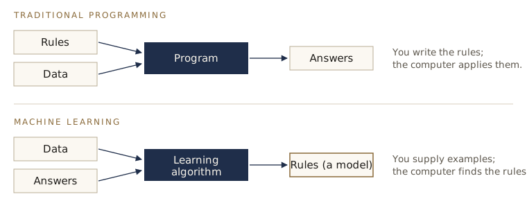
Suppose you want a program that recognizes cracks in photographs of a concrete beam. Writing the rules by hand (“a crack is a dark line at least 40 pixels long, unless it is a shadow, unless…”) breaks down quickly. With machine learning you collect a few thousand photos, label each one crack or no crack, and let a model learn what separates them.
When to use machine learning, and when not to
Machine learning is a good fit when
- the rules are too many or too subtle to write down (recognizing a face, reading handwriting);
- the environment keeps changing and the program needs to adapt to new data;
- there is a large amount of data and you want to find patterns in it.
It is usually a poor fit when
- a simple rule-based program already solves the problem — if you can write the rule, write the rule;
- you must be able to explain exactly why each decision was made (the patterns a deep model learns are hard to read);
- errors are unacceptable, since every learned model is wrong some of the time;
- you have very little data.
The kinds of learning you will meet
- Supervised learning — every training example comes with the right answer (a label). Most of this course is supervised: images with their class names, measurements with the value to predict.
- Unsupervised and self-supervised learning — there are no labels; the model finds structure on its own, such as groups of similar customers. Large language models are pretrained this way, by predicting the next word of ordinary text.
- Transfer learning — start from a model that already learned something useful on a large dataset and adapt it to your problem. It is one of the most practical ideas in the field, and module 06 is devoted to it.
What a neural network actually does
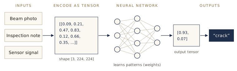
Whatever the data, the recipe is the same: turn the inputs into numbers, pass the numbers through a network that learns patterns in them, and turn the network’s output numbers back into something a person can use.
What PyTorch is
PyTorch is an open-source library for building and training neural networks in Python. It gives you three things you would otherwise have to write yourself: a fast data structure for numbers (the tensor), the ability to run the arithmetic on a graphics card (GPU), and automatic calculation of the gradients a model needs in order to learn. It is widely used in both research and industry, so what you learn here carries directly into the tools practitioners use.
Setting up
We will work in Google Colab, a free notebook that runs in the browser with PyTorch already installed. A notebook is a document made of cells: you type Python into a cell, press Shift + Enter, and the result appears underneath.
- Go to colab.research.google.com and choose New notebook.
- In the menu, choose Runtime → Change runtime type and pick a GPU. You will not need it until the end of this module, but it costs nothing to turn on now.
- In the first cell, import PyTorch and print its version:
import torch
torch.__version__
'2.14.0+cu130'
Your version number will probably differ; anything from 2.0 onward works for this course. The +cu130 part means this build of PyTorch can use NVIDIA GPUs.
Note. In the code below, lines that start with
#are comments. Python ignores them; they are there for you. The box under a code cell, labeled Output, shows what the cell prints.
Tensors
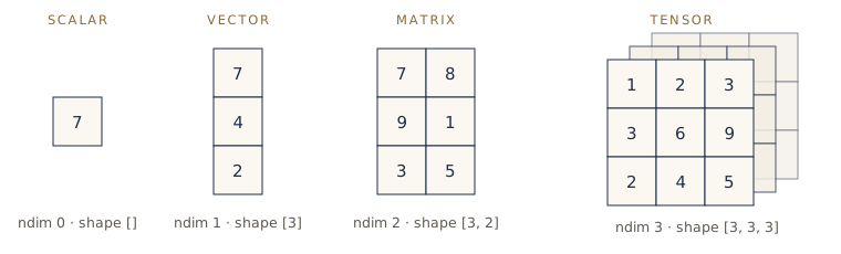
A tensor is a grid of numbers with any number of dimensions. You already know the first few kinds:
torch.Tensor; only the number of dimensions differs.Scalars, vectors, and matrices
A scalar is a single number. It has zero dimensions.
scalar = torch.tensor(7)
scalar
tensor(7)
scalar.ndim
0
To get the plain Python number back out of a one-element tensor, use .item():
scalar.item()
7
A vector is a list of numbers. It has one dimension. A vector can describe one thing with several numbers — for example a beam’s [length, width, depth] in meters.
vector = torch.tensor([7, 7])
vector.ndim, vector.shape
(1, torch.Size([2]))
Two attributes will come up constantly. ndim counts the dimensions. shape says how many elements lie along each one. A quick way to count dimensions by eye: count the opening square brackets at the start.
A matrix has two dimensions — rows and columns, like a spreadsheet.
MATRIX = torch.tensor([[7, 8],
                       [9, 10]])
MATRIX.ndim, MATRIX.shape
(2, torch.Size([2, 2]))
Tensors with three or more dimensions
Anything with more dimensions we simply call a tensor.
TENSOR = torch.tensor([[[1, 2, 3],
                        [3, 6, 9],
                        [2, 4, 5]]])
TENSOR.ndim, TENSOR.shape
(3, torch.Size([1, 3, 3]))
Read the shape from the outside in: one block, containing three rows, each with three numbers. The first dimension is the outermost bracket.
A color photograph is a natural three-dimensional tensor: three color channels (red, green, blue), each a grid of pixel intensities of a given height and width. A 224 × 224 photo is a tensor of shape [3, 224, 224], and a batch of 32 such photos is a four-dimensional tensor of shape [32, 3, 224, 224]. You will meet shapes like these again in module 03.
Note. By convention, scalars and vectors get lower-case names (
y,a) and matrices and higher tensors get upper-case names (X,W). PyTorch does not care, but it makes code easier to read.
Creating tensors
You will rarely type tensors out by hand. More often you create them with a function, or load them from data.
Random tensors
A neural network starts life as tensors full of random numbers and then adjusts them, a little at a time, until they describe the data well. That is what “training” means:
start with random numbers → look at data → update the numbers → look at more data → update again
random_tensor = torch.rand(size=(3, 4))
random_tensor, random_tensor.dtype
(tensor([[0.6709, 0.7096, 0.1050, 0.3310],
        [0.2577, 0.1638, 0.7138, 0.2757],
        [0.3083, 0.1421, 0.0624, 0.5003]]), torch.float32)
torch.rand draws numbers evenly between 0 and 1. Your numbers will differ from these — they are random. We will make them repeatable later in this module.
A random tensor shaped like a color image:
random_image = torch.rand(size=(3, 224, 224))
random_image.shape, random_image.ndim
(torch.Size([3, 224, 224]), 3)
Zeros, ones, and ranges
zeros = torch.zeros(size=(3, 4))
ones = torch.ones(size=(3, 4))
zeros, ones.dtype
(tensor([[0., 0., 0., 0.],
        [0., 0., 0., 0.],
        [0., 0., 0., 0.]]), torch.float32)
torch.arange(start, end, step) counts from start up to, but not including, end:
zero_to_ten = torch.arange(start=0, end=10, step=1)
zero_to_ten
tensor([0, 1, 2, 3, 4, 5, 6, 7, 8, 9])
And to make a tensor the same shape as another one, use the _like functions:
ten_zeros = torch.zeros_like(input=zero_to_ten)
ten_zeros
tensor([0, 0, 0, 0, 0, 0, 0, 0, 0, 0])
Datatypes
Every tensor has a datatype (dtype) that says how each number is stored. The default for decimals is torch.float32 — a 32-bit floating-point number. Whole numbers default to torch.int64.
float_32_tensor = torch.tensor([3.0, 6.0, 9.0])
int_tensor = torch.tensor([3, 6, 9])
float_32_tensor.dtype, int_tensor.dtype
(torch.float32, torch.int64)
Lower precision, such as torch.float16, uses half the memory and runs faster on modern GPUs, at the cost of less exact numbers. You can convert with .type() (or the equivalent .to()):
float_16_tensor = float_32_tensor.type(torch.float16)
float_16_tensor
tensor([3., 6., 9.], dtype=torch.float16)
The three questions to ask of any tensor
Nearly every error you will hit in this course comes down to one of three mismatches: the tensors have the wrong shape, the wrong datatype, or live on the wrong device (CPU or GPU). So when something breaks, print these three attributes first:
some_tensor = torch.rand(3, 4)
print(f"Shape:    {some_tensor.shape}")
print(f"Datatype: {some_tensor.dtype}")
print(f"Device:   {some_tensor.device}")
Shape:    torch.Size([3, 4])
Datatype: torch.float32
Device:   cpu
Habit. Before combining two tensors, ask: what shape, what datatype, what device? This one habit will save you hours.
Arithmetic on tensors
Element-wise operations
The basic operators work element by element: each number is combined with the number in the same position.
tensor = torch.tensor([1, 2, 3])
print(tensor + 10)
print(tensor * 10)
print(tensor - 10)
print(tensor * tensor)
tensor([11, 12, 13])
tensor([10, 20, 30])
tensor([-9, -8, -7])
tensor([1, 4, 9])
Note that tensor + 10 added 10 to every element even though 10 is a single number. PyTorch stretches the smaller operand to match the larger one — a rule called broadcasting. It is convenient, and occasionally surprising; the broadcasting rules are worth a read once you are comfortable.
Operations return a new tensor and leave the original alone unless you reassign it:
tensor
tensor([1, 2, 3])
Matrix multiplication
The most important operation in deep learning is matrix multiplication (PyTorch: torch.matmul, or the @ operator). Most of the work inside a neural network is matrix multiplications.
It is not element-wise. Each entry of the result is a row of the first matrix combined with a column of the second: multiply them pair by pair and add up the products.
print("Element-wise:", tensor * tensor)
print("Matrix multiplication:", torch.matmul(tensor, tensor))
Element-wise: tensor([1, 4, 9])
Matrix multiplication: tensor(14)
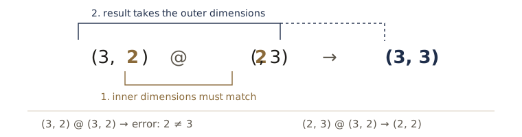
For two vectors, matrix multiplication gives \(1 \times 1 + 2 \times 2 + 3 \times 3 = 14\) — the dot product. For matrices there are two rules to remember:
- The inner dimensions must match.
(3, 2) @ (2, 3)works.(3, 2) @ (3, 2)does not. - The result has the shape of the outer dimensions.
(3, 2) @ (2, 3)gives(3, 3);(2, 3) @ (3, 2)gives(2, 2).
Why not just write a loop? Because PyTorch’s built-in version is enormously faster. Compare a hand-written loop with torch.matmul on 1,000-element vectors:
import time

a = torch.rand(1000)
b = torch.rand(1000)

start = time.perf_counter()
value = 0
for i in range(len(a)):
    value += a[i] * b[i]
loop_time = time.perf_counter() - start

start = time.perf_counter()
value = torch.matmul(a, b)
matmul_time = time.perf_counter() - start

print(f"Python loop:  {loop_time * 1000:.2f} ms")
print(f"torch.matmul: {matmul_time * 1000:.3f} ms")
Python loop:  5.22 ms
torch.matmul: 0.094 ms
Exact times depend on your machine, but the built-in version is dozens to hundreds of times faster — and the gap grows with the size of the tensors. The lesson generalizes: avoid Python loops over tensor elements; use tensor operations instead.
Shape errors, and how to fix them
Here is the error you will see more than any other:
tensor_A = torch.tensor([[1, 2],
                         [3, 4],
                         [5, 6]], dtype=torch.float32)

tensor_B = torch.tensor([[7, 10],
                         [8, 11],
                         [9, 12]], dtype=torch.float32)
torch.matmul(tensor_A, tensor_B)
RuntimeError: mat1 and mat2 shapes cannot be multiplied (3x2 and 3x2)
Both are (3, 2), so the inner dimensions (2 and 3) do not match. The fix is to transpose one of them — swap its rows and columns — with .T:
print(f"tensor_A: {tensor_A.shape},  tensor_B.T: {tensor_B.T.shape}")
output = torch.matmul(tensor_A, tensor_B.T)
print(output)
print(f"Output shape: {output.shape}")
tensor_A: torch.Size([3, 2]),  tensor_B.T: torch.Size([2, 3])
tensor([[ 27.,  30.,  33.],
        [ 61.,  68.,  75.],
        [ 95., 106., 117.]])
Output shape: torch.Size([3, 3])
Where this shows up: a linear layer
The simplest building block of a neural network, torch.nn.Linear, is exactly a matrix multiplication plus a bias:
Here \(x\) is the input, \(A\) is a matrix of weights the layer learns, and \(b\) is a bias vector it also learns. Watch the shapes:
torch.manual_seed(42)
linear = torch.nn.Linear(in_features=2, out_features=6)  # 2 numbers in, 6 numbers out
x = tensor_A                                             # 3 examples with 2 numbers each
output = linear(x)
print(f"Input shape:  {x.shape}")
print(f"Output shape: {output.shape}")
Input shape:  torch.Size([3, 2])
Output shape: torch.Size([3, 6])
Three examples went in with two numbers each; three came out with six numbers each. Changing out_features changes the output shape — and the inner dimension, in_features, must match the last dimension of the input. That is rule 1 again.
Summarizing a tensor
Finding the minimum, maximum, mean, and sum is called aggregation.
x = torch.arange(0, 100, 10)
x
tensor([ 0, 10, 20, 30, 40, 50, 60, 70, 80, 90])
print(f"Minimum: {x.min()}")
print(f"Maximum: {x.max()}")
print(f"Mean:    {x.type(torch.float32).mean()}")
print(f"Sum:     {x.sum()}")
Minimum: 0
Maximum: 90
Mean:    45.0
Sum:     450
mean() needs a floating-point tensor; calling it on integers raises a datatype error, which is why we converted first. Often you want the position of the largest value rather than the value itself — for instance, to find which class a model rates most likely. That is argmax (and argmin):
print(f"Index of max: {x.argmax()}")
print(f"Index of min: {x.argmin()}")
Index of max: 9
Index of min: 0
Changing a tensor’s shape
Different layers expect different shapes, so a lot of deep learning code is rearranging tensors without changing their values.
| Method | What it does |
|---|---|
x.reshape(shape) |
Rearranges x into a new shape with the same number of elements |
x.view(shape) |
Like reshape, but shares memory with the original |
torch.stack(tensors, dim) |
Joins a list of same-shaped tensors along a new dimension |
x.squeeze() |
Removes all dimensions of size 1 |
x.unsqueeze(dim) |
Adds a dimension of size 1 at position dim |
x.permute(dims) |
Reorders the dimensions |
x = torch.arange(1., 8.)
x, x.shape
(tensor([1., 2., 3., 4., 5., 6., 7.]), torch.Size([7]))
reshape needs the new shape to hold the same number of elements (here 7):
x_reshaped = x.reshape(1, 7)
x_reshaped, x_reshaped.shape
(tensor([[1., 2., 3., 4., 5., 6., 7.]]), torch.Size([1, 7]))
view does the same, but the result shares memory with the original — change one and the other changes too:
z = x.view(1, 7)
z[:, 0] = 5
z, x
(tensor([[5., 2., 3., 4., 5., 6., 7.]]), tensor([5., 2., 3., 4., 5., 6., 7.]))
stack puts tensors on top of each other along a new dimension:
x_stacked = torch.stack([x, x, x, x], dim=0)
x_stacked.shape
torch.Size([4, 7])
squeeze removes dimensions of size 1, and unsqueeze adds one back:
print(f"Before squeeze: {x_reshaped.shape}")
x_squeezed = x_reshaped.squeeze()
print(f"After squeeze:  {x_squeezed.shape}")
x_unsqueezed = x_squeezed.unsqueeze(dim=0)
print(f"After unsqueeze(dim=0): {x_unsqueezed.shape}")
Before squeeze: torch.Size([1, 7])
After squeeze:  torch.Size([7])
After unsqueeze(dim=0): torch.Size([1, 7])
permute reorders dimensions. Its most common use is images: image libraries store pictures as height × width × color channels, but PyTorch layers expect channels × height × width.
x_original = torch.rand(size=(224, 224, 3))   # [height, width, channels]
x_permuted = x_original.permute(2, 0, 1)      # [channels, height, width]
print(f"Original: {x_original.shape}")
print(f"Permuted: {x_permuted.shape}")
Original: torch.Size([224, 224, 3])
Permuted: torch.Size([3, 224, 224])
Watch out.
viewandpermutereturn a new view of the same memory, not a copy. Changing the values in the view changes the original.
Selecting data (indexing)
Indexing works as it does for Python lists, with one index per dimension, counting from 0.
x = torch.arange(1, 10).reshape(1, 3, 3)
x, x.shape
(tensor([[[1, 2, 3],
         [4, 5, 6],
         [7, 8, 9]]]), torch.Size([1, 3, 3]))
Go in one bracket at a time:
print(f"x[0]:       {x[0]}")
print(f"x[0][0]:    {x[0][0]}")
print(f"x[0][0][0]: {x[0][0][0]}")
x[0]:       tensor([[1, 2, 3],
        [4, 5, 6],
        [7, 8, 9]])
x[0][0]:    tensor([1, 2, 3])
x[0][0][0]: 1
A colon : means “everything along this dimension”:
print(x[:, 0])       # every block, first row
print(x[:, :, 1])    # every block, every row, second column
print(x[0, 2, 2])    # first block, third row, third column
tensor([[1, 2, 3]])
tensor([[2, 5, 8]])
tensor(9)
PyTorch and NumPy
NumPy is Python’s standard library for numerical arrays, and much scientific data starts life as a NumPy array. Two functions move between them:
torch.from_numpy(array)— NumPy array → PyTorch tensortensor.numpy()— PyTorch tensor → NumPy array
import numpy as np

array = np.arange(1.0, 8.0)
tensor = torch.from_numpy(array)
array, tensor
(array([1., 2., 3., 4., 5., 6., 7.]), tensor([1., 2., 3., 4., 5., 6., 7.], dtype=torch.float64))
Watch out. NumPy’s default decimal type is
float64, and the tensor keeps it. PyTorch models expectfloat32, so convert withtorch.from_numpy(array).type(torch.float32)— otherwise you will meet a datatype error.
tensor = torch.ones(7)
numpy_tensor = tensor.numpy()
tensor, numpy_tensor
(tensor([1., 1., 1., 1., 1., 1., 1.]), array([1., 1., 1., 1., 1., 1., 1.], dtype=float32))
Reproducibility: taming randomness
Randomness is essential to training, but when you are debugging, or sharing results with a classmate, you want the same “random” numbers every time. Computers produce pseudo-random numbers from a starting value called a seed; fix the seed and you fix the sequence.
random_tensor_A = torch.rand(3, 4)
random_tensor_B = torch.rand(3, 4)
print(torch.equal(random_tensor_A, random_tensor_B))

RANDOM_SEED = 42
torch.manual_seed(RANDOM_SEED)
random_tensor_C = torch.rand(3, 4)

torch.manual_seed(RANDOM_SEED)   # reset the seed before each call you want repeated
random_tensor_D = torch.rand(3, 4)
print(torch.equal(random_tensor_C, random_tensor_D))
False
True
The seed has to be reset before each call you want repeated, because every call moves the generator along. In this course we set torch.manual_seed(42) at the start of experiments so that your numbers match the notes. (Full reproducibility on GPUs needs a few more settings; see PyTorch’s reproducibility notes.)
Running on a GPU
Deep learning is mostly matrix multiplication, and a graphics card (GPU) can do thousands of multiplications at once. Training that takes hours on a CPU can take minutes on a GPU. In Colab you switched one on in the setup step; check that PyTorch can see it:
torch.cuda.is_available()
False
That prints True on a Colab GPU runtime (it printed False here because these notes were run on a CPU). NVIDIA GPUs are reached through a library called CUDA; on recent Macs PyTorch can use the built-in Apple GPU through a backend called mps.
Device-agnostic code
Since your code may run on a laptop, on Colab, or on a lab server, write it so it uses a GPU when one exists and falls back to the CPU otherwise. This line appears at the top of every notebook from here on:
device = "cuda" if torch.cuda.is_available() else "cpu"
device
'cpu'
Move a tensor (and later, a whole model) to the device with .to(device):
tensor = torch.tensor([1, 2, 3])
tensor_on_device = tensor.to(device)
tensor_on_device, tensor_on_device.device
(tensor([1, 2, 3]), device(type='cpu'))
On a GPU the output reads device='cuda:0' — the first GPU. Note that .to() returns a new tensor on the target device and leaves the original where it was, so assign the result to a name, as above.
Getting data back to the CPU
NumPy only works on the CPU. To convert a GPU tensor to NumPy, bring it back first with .cpu():
tensor_back_on_cpu = tensor_on_device.cpu().numpy()
tensor_back_on_cpu
array([1, 2, 3])
Calling .numpy() directly on a GPU tensor raises TypeError: can't convert cuda:0 device type tensor to numpy — the wrong device error from our three questions.
Summary
| Task | Code |
|---|---|
| Make a tensor | torch.tensor(data), torch.rand(shape), torch.zeros(shape), torch.arange(start, end) |
| Inspect it | x.ndim, x.shape, x.dtype, x.device |
| Change datatype | x.type(torch.float32) |
| Element-wise math | x + y, x * y |
| Matrix multiplication | torch.matmul(x, y) or x @ y; inner dimensions must match |
| Summaries | x.min(), x.max(), x.mean(), x.sum(), x.argmax() |
| Reshape | x.reshape, x.view, torch.stack, x.squeeze, x.unsqueeze, x.permute |
| NumPy | torch.from_numpy(a), x.numpy() |
| Reproducibility | torch.manual_seed(42) |
| Devices | device = "cuda" if torch.cuda.is_available() else "cpu", x.to(device), x.cpu() |
Three ideas to carry into the next module: a neural network is a stack of tensor operations; its learnable numbers start random and are gradually improved; and most errors are a mismatch in shape, datatype, or device.
Exercises
Do these in a fresh Colab notebook. They take about an hour.
- Read the documentation. Spend ten minutes on the pages for
torch.Tensorand CUDA semantics. You are aiming for awareness, not full understanding. - Create a random tensor of shape
(7, 7). - Matrix-multiply it with a random tensor of shape
(1, 7). (Hint: one of them needs transposing.) What is the output shape, and why? - Set the seed to
0and repeat exercises 2 and 3. Run the cell twice and confirm you get the same numbers. - Is there a GPU equivalent of
torch.manual_seed()? Find it in the documentation and set the GPU seed to1234. - With
torch.manual_seed(1234), create two random tensors of shape(2, 3)and send them to the GPU (use a Colab GPU runtime). - Matrix-multiply the tensors from exercise 6, adjusting one shape as needed. Then find the maximum and minimum of the result, and the positions of each.
- Create a random tensor of shape
(1, 1, 1, 10)with seed7, then remove all the size-1 dimensions to get shape[10]. Print both tensors and their shapes. - In your own words. For a problem from your engineering field, write three sentences: what the inputs would be as tensors (with shapes), what the model should output, and whether a hand-written rule could do the job instead.
Going further
- The PyTorch tensors tutorial covers the same ground from a different angle.
- Broadcasting semantics — the exact rules for combining tensors of different shapes.
- If matrix multiplication still feels mechanical, work a
(2, 3) @ (3, 2)example by hand on paper, then check it withtorch.matmul.
These notes follow the path of Daniel Bourke's Learn PyTorch for Deep Learning (MIT license), rewritten for engineering students meeting Python and machine learning for the first time.