CSE 676 · Module 05 · Week 3
Single-layer Networks: Classification
Discriminant functions, decision theory and ROC curves, generative classifiers, logistic and softmax regression, probit regression, and canonical link functions.
Companion reading: Bishop & Bishop, Deep Learning: Foundations and Concepts, chapter 5, “Single-layer Networks: Classification”
By the end of this module you can
- Explain the geometry of a linear discriminant — why \(\mathbf{w}\) is normal to the decision boundary and why \(y(\mathbf{x})/\lVert \mathbf{w} \rVert\) is a signed distance — and why \(K\) linear functions avoid the ambiguous regions of one-versus-the-rest and one-versus-one schemes.
- Fit a least-squares classifier and show on your own data how outliers and a sandwiched middle class break it.
- Turn posterior probabilities into decisions that minimize the misclassification rate or an expected loss, with or without a reject option.
- Compute a confusion matrix, precision, recall, and the F-score for an imbalanced problem, and build an ROC curve and its AUC, checking the AUC against the pairwise-ranking definition.
- Derive the linear logit of a Gaussian generative classifier with shared covariance, fit it by maximum likelihood, and build a naive Bayes classifier for binary features.
- Train logistic and softmax regression by gradient descent with a numerically stable log-softmax, and verify every gradient by finite differences.
- Read logistic and softmax regression as single-layer networks and explain, through canonical link functions, why the gradient for each weight is the output error \(y_k - t_k\) times the input feeding that weight.
- Compare probit and logistic regression, including how their tails respond to mislabeled points.
Contents
- Discriminant functions
- Decision theory
- Generative classifiers
- Discriminative classifiers
- Summary
- Exercises
- Going further
Module 04 built a regression model as a network with one layer of weights: a vector of basis functions \(\boldsymbol{\phi}(\mathbf{x})\) goes in, a weighted sum comes out, and the sum-of-squares error measures the fit. This module keeps the layer and changes the target. The output is now one of \(K\) discrete classes, and that single change raises three questions that regression never asked: how to encode a class as a target, what function to put on the output so that it can be read as a probability, and which error function belongs with that output.
The answers are the ones every deep classifier uses. A logistic sigmoid (two classes) or a softmax (\(K\) classes) sits on the output, the error is the cross-entropy, which is the negative log likelihood of the labels, and with that pairing the gradient of the error with respect to any weight is the output error \(y_k - t_k\) times the input that feeds the weight. In module 06 the fixed features become learned hidden units, and in module 08 backpropagation sends exactly this \(y_k - t_k\) backward through the network. The output layer itself never changes. The single-layer models of this module are the last layer of every classifier in the rest of the course.
We follow chapter 5 of Bishop & Bishop: discriminant functions and least squares; decision theory, meaning how to turn probabilities into decisions and how to measure a classifier; generative classifiers, where a linear model of the posterior falls out of assumptions about the data; and discriminative classifiers, where logistic, softmax, and probit regression are fitted directly. Much of the material also appears in Intro to ML, module 04, which goes further into Fisher’s discriminant, the perceptron, Newton’s method, and Bayesian logistic regression. Here we keep the shared derivations short, link there for the long versions, and spend the space on the network view and on how classifiers are evaluated.
import numpy as np
from scipy.special import expit, logsumexp, erf, log_ndtr
from scipy import stats                      # used only to check our own code

np.set_printoptions(precision=4, suppress=True)
rng = np.random.default_rng(505)

def add_bias(X):
    """Prepend the dummy input x_0 = 1 to every row: shape (N, D) -> (N, D + 1)."""
    return np.column_stack([np.ones(len(X)), X])

def one_hot(labels, K):
    """1-of-K coding: row n is t_n^T, a single 1 in column labels[n]."""
    return np.eye(K)[labels]
In code, classes are numbered from 0, so label k stands for class \(\mathcal{C}_{k+1}\). For two-class problems we use a target t that is 1 for \(\mathcal{C}_1\) and 0 for \(\mathcal{C}_2\).
Discriminant functions
A classifier divides input space into decision regions \(\mathcal{R}_k\), one per class, and every input in \(\mathcal{R}_k\) is assigned to \(\mathcal{C}_k\). The surfaces between regions are the decision boundaries. In this module the boundaries are hyperplanes, flat surfaces of dimension \(D - 1\) in the \(D\)-dimensional input space, and we call such classifiers linear. A data set whose classes can be split without error by hyperplanes is linearly separable.
A discriminant function maps an input straight to a class, with no probabilities involved. It is the simplest of the three approaches to classification we will meet, and its geometry carries over to the others.
Two classes
The linear discriminant for two classes is
\[y(\mathbf{x}) = \mathbf{w}^{\mathrm{T}}\mathbf{x} + w_0,\]with weight vector \(\mathbf{w}\) and bias \(w_0\) (a parameter, not the statistical bias of module 04). We assign \(\mathbf{x}\) to \(\mathcal{C}_1\) when \(y(\mathbf{x}) \geq 0\) and to \(\mathcal{C}_2\) otherwise, so the decision boundary is the hyperplane \(y(\mathbf{x}) = 0\).
Two facts about this hyperplane explain what the parameters do.
The weights set the orientation. Take two points \(\mathbf{x}_A, \mathbf{x}_B\) on the boundary. Subtracting \(y(\mathbf{x}_A) = 0\) from \(y(\mathbf{x}_B) = 0\) gives \(\mathbf{w}^{\mathrm{T}}(\mathbf{x}_B - \mathbf{x}_A) = 0\): \(\mathbf{w}\) is orthogonal to every direction lying in the boundary, so it is the boundary’s normal. For a point \(\mathbf{x}\) on the boundary, \(\mathbf{w}^{\mathrm{T}}\mathbf{x}/\lVert\mathbf{w}\rVert = -w_0/\lVert\mathbf{w}\rVert\), so the bias fixes how far the hyperplane sits from the origin.
The output is a scaled distance. Write any point as its orthogonal projection \(\mathbf{x}_{\perp}\) onto the boundary plus a step of signed length \(r\) along the unit normal, \(\mathbf{x} = \mathbf{x}_{\perp} + r\,\mathbf{w}/\lVert\mathbf{w}\rVert\). Multiply by \(\mathbf{w}^{\mathrm{T}}\), add \(w_0\), and use \(y(\mathbf{x}_{\perp}) = 0\):
\[y(\mathbf{x}) = r\,\frac{\mathbf{w}^{\mathrm{T}}\mathbf{w}}{\lVert\mathbf{w}\rVert} = r\,\lVert\mathbf{w}\rVert \qquad\Longrightarrow\qquad r = \frac{y(\mathbf{x})}{\lVert\mathbf{w}\rVert}.\]The output of a linear discriminant is the signed distance to the boundary, measured in units of \(1/\lVert\mathbf{w}\rVert\). Scaling \(\mathbf{w}\) and \(w_0\) together leaves the boundary where it is but makes the outputs larger; we will see this freedom again when logistic regression meets separable data.
w_d, w0_d = np.array([2.0, -1.0]), 1.5
X_pts = rng.normal(size=(4, 2))
r = (X_pts @ w_d + w0_d) / np.linalg.norm(w_d)                 # r = y(x) / ||w||
X_perp = X_pts - r[:, None] * w_d / np.linalg.norm(w_d)       # step back along the normal
print("signed distances r:          ", r)
print("y at the projections:        ", X_perp @ w_d + w0_d)
print("lengths ||x - x_perp||:      ", np.linalg.norm(X_pts - X_perp, axis=1))
print(f"offset of boundary from origin: {-w0_d / np.linalg.norm(w_d):.4f}")
signed distances r:           [2.3684 1.7766 0.5462 1.5469]
y at the projections:         [0. 0. 0. 0.]
lengths ||x - x_perp||:       [2.3684 1.7766 0.5462 1.5469]
offset of boundary from origin: -0.6708
The projections land exactly on the boundary, and the distances to them equal \(\lvert r\rvert\). As in module 04, it is often tidier to absorb the bias by adding a dummy input \(x_0 = 1\): with \(\widetilde{\mathbf{w}} = (w_0, \mathbf{w})\) and \(\widetilde{\mathbf{x}} = (1, \mathbf{x})\), the discriminant is \(y(\mathbf{x}) = \widetilde{\mathbf{w}}^{\mathrm{T}}\widetilde{\mathbf{x}}\), a hyperplane through the origin of the \((D+1)\)-dimensional augmented space. That is what add_bias does.
Multiple classes
For \(K > 2\) classes it is tempting to reuse two-class discriminants. There are two obvious ways, and both leave parts of the input space without a clear answer.
- One-versus-the-rest. Train one discriminant per class to separate \(\mathcal{C}_k\) from everything else (\(K - 1\) of them suffice in principle). Where no discriminant claims a point, or two claim it, the class is undefined.
- One-versus-one. Train \(K(K-1)/2\) discriminants, one per pair of classes, and let them vote. Three pairwise boundaries that do not meet in a single point enclose a region where every class gets exactly one vote.
The cell below makes both problems concrete. Three classes sit at the corners of a triangle; the one-versus-the-rest discriminants are the nearest-mean rules “closer to \(\boldsymbol{\mu}_k\) than to the average of the other two means”, and the pairwise discriminants are the perpendicular bisectors of each pair of means, each shifted a little toward one class of its pair (\(\mathcal{C}_2\) gains ground on \(\mathcal{C}_1\), \(\mathcal{C}_3\) on \(\mathcal{C}_2\), \(\mathcal{C}_1\) on \(\mathcal{C}_3\)), as happens when each pair is trained on its own data.
mus = np.array([[0.0, 2.0], [-2.0, -1.0], [2.0, -1.0]])        # three class centers
g = np.linspace(-4, 4, 400)
G = np.array(np.meshgrid(g, g)).reshape(2, -1).T               # grid over the square

def bisector(a, b, shift=0.0):
    """Linear discriminant that is positive on a's side of the perpendicular bisector."""
    return lambda X: X @ (a - b) - 0.5 * (a @ a - b @ b) + shift

# one-versus-the-rest: class k against the mean of the other two centers
rest = [bisector(mus[k], np.delete(mus, k, axis=0).mean(axis=0)) for k in range(3)]
claims = np.stack([f(G) > 0 for f in rest], axis=1).sum(axis=1)
print(f"one-vs-rest:  no class {np.mean(claims == 0):.1%},  "
      f"two or more {np.mean(claims >= 2):.1%}")

# one-versus-one: majority vote over the three pairwise discriminants
votes = np.zeros((len(G), 3), dtype=int)
for j, k in [(0, 1), (1, 2), (2, 0)]:
    win_j = bisector(mus[j], mus[k], shift=-2.0)(G) > 0         # nudged toward class k
    votes[:, j] += win_j
    votes[:, k] += ~win_j
print(f"one-vs-one:   three-way tie {np.mean(votes.max(axis=1) == 1):.1%}")

# K linear functions y_k(x) = w_k^T x + w_k0, decided by the largest
Y = G @ mus.T - 0.5 * np.sum(mus**2, axis=1)
n_best = np.sum(Y == Y.max(axis=1, keepdims=True), axis=1)
print(f"K-class rule: exactly one class {np.mean(n_best == 1):.1%}")
one-vs-rest:  no class 2.4%,  two or more 30.6%
one-vs-one:   three-way tie 2.3%
K-class rule: exactly one class 100.0%
Almost a third of the square is claimed by two one-versus-the-rest discriminants at once, and a small triangle in the middle gets exactly one vote per class under one-versus-one. A single \(K\)-class discriminant avoids the trouble. Use \(K\) linear functions
\[y_k(\mathbf{x}) = \mathbf{w}_k^{\mathrm{T}}\mathbf{x} + w_{k0}, \qquad k = 1, \dots, K,\]and assign \(\mathbf{x}\) to the class with the largest \(y_k\). Every point gets exactly one class (ties have probability zero). The boundary between \(\mathcal{R}_k\) and \(\mathcal{R}_j\) is where \(y_k = y_j\), the hyperplane \((\mathbf{w}_k - \mathbf{w}_j)^{\mathrm{T}}\mathbf{x} + (w_{k0} - w_{j0}) = 0\), so everything we said about two classes applies to each pair.
The regions are also convex. If \(\mathbf{x}_A\) and \(\mathbf{x}_B\) are both in \(\mathcal{R}_k\), any point between them is \(\widehat{\mathbf{x}} = \lambda\mathbf{x}_A + (1 - \lambda)\mathbf{x}_B\) with \(0 \leq \lambda \leq 1\), and by linearity \(y_k(\widehat{\mathbf{x}}) = \lambda y_k(\mathbf{x}_A) + (1-\lambda)y_k(\mathbf{x}_B)\). The same holds for every \(y_j\), and since \(y_k > y_j\) at both ends, it holds in between. Convexity is a limitation as well as a comfort: a single-layer network can never give one class two separate regions. Getting past that is the job of hidden layers.
1-of-K coding
To fit a classifier we need numeric targets. For two classes, a single binary target \(t \in \{0, 1\}\) does the job, with \(t = 1\) meaning \(\mathcal{C}_1\). It can be read as the probability that the class is \(\mathcal{C}_1\), a probability that for a labeled example is exactly 0 or 1. For \(K\) classes we use 1-of-\(K\) coding, also called one-hot encoding: \(\mathbf{t}\) is a vector of \(K\) zeros with a single 1 in position \(k\) for class \(\mathcal{C}_k\). With \(K = 4\), class \(\mathcal{C}_3\) has target \((0, 0, 1, 0)^{\mathrm{T}}\), and again \(t_k\) reads as the probability of class \(\mathcal{C}_k\). one_hot builds these rows; in deep learning libraries the same coding is usually implied, and the loss functions accept integer labels directly.
Least squares for classification
Least squares gave regression a closed-form fit, so it is natural to try it here. Give each class its own linear output, collect the augmented weight vectors \(\widetilde{\mathbf{w}}_k\) as the columns of a \((D+1) \times K\) matrix \(\widetilde{\mathbf{W}}\), and write \(\mathbf{y}(\mathbf{x}) = \widetilde{\mathbf{W}}^{\mathrm{T}}\widetilde{\mathbf{x}}\). With the augmented inputs as the rows of \(\widetilde{\mathbf{X}}\) and the one-hot targets as the rows of \(\mathbf{T}\), the sum-of-squares error
\[E_D(\widetilde{\mathbf{W}}) = \frac{1}{2}\operatorname{Tr}\left\{(\widetilde{\mathbf{X}}\widetilde{\mathbf{W}} - \mathbf{T})^{\mathrm{T}}(\widetilde{\mathbf{X}}\widetilde{\mathbf{W}} - \mathbf{T})\right\}\]is \(K\) separate regressions that share one design matrix. Setting the gradient \(\widetilde{\mathbf{X}}^{\mathrm{T}}(\widetilde{\mathbf{X}}\widetilde{\mathbf{W}} - \mathbf{T})\) to zero gives
\[\widetilde{\mathbf{W}} = (\widetilde{\mathbf{X}}^{\mathrm{T}}\widetilde{\mathbf{X}})^{-1}\widetilde{\mathbf{X}}^{\mathrm{T}}\mathbf{T} = \widetilde{\mathbf{X}}^{\dagger}\mathbf{T},\]with \(\widetilde{\mathbf{X}}^{\dagger}\) the pseudo-inverse from module 04. A new input goes to the class with the largest output.
There is a reason to hope this works. Least squares estimates the conditional mean \(\mathbb{E}[\mathbf{t} \mid \mathbf{x}]\), and for one-hot targets that mean is the vector of posterior class probabilities (exercise 1). The outputs even sum to one for every \(\mathbf{x}\): whenever all training targets satisfy a linear constraint \(\mathbf{a}^{\mathrm{T}}\mathbf{t}_n + b = 0\), and the model has a bias, the least-squares predictions satisfy it too (Bishop & Bishop exercise 5.3; Intro to ML, module 04 has the two-line proof). One-hot targets satisfy \(\mathbf{1}^{\mathrm{T}}\mathbf{t}_n - 1 = 0\). But nothing keeps the outputs inside \((0, 1)\), and the approximation to the posteriors is poor. Two experiments show how poor.
The first has three classes whose centers lie roughly on a line, 60 points each.
def fit_least_squares(X, T):
    """W~ = pinv(X~) T, solved with lstsq. Returns shape (D + 1, K) (or (D + 1,))."""
    W, *_ = np.linalg.lstsq(add_bias(X), T, rcond=None)
    return W

rng3 = np.random.default_rng(53)
means3 = np.array([[-4.0, 1.0], [0.0, 0.0], [4.0, -1.0]])
X3 = np.vstack([rng3.normal(m, 1.0, size=(60, 2)) for m in means3])
lab3 = np.repeat(np.arange(3), 60)
T3 = one_hot(lab3, 3)

W_ls3 = fit_least_squares(X3, T3)
Y_ls3 = add_bias(X3) @ W_ls3
pred_ls3 = Y_ls3.argmax(axis=1)
print(f"outputs sum to one: largest deviation {np.abs(Y_ls3.sum(axis=1) - 1).max():.1e}")
print(f"outputs range over [{Y_ls3.min():.2f}, {Y_ls3.max():.2f}] on the training data")
print(f"training errors: {np.sum(pred_ls3 != lab3)} of {len(lab3)};  "
      f"points given to each class: {np.bincount(pred_ls3, minlength=3)}")
outputs sum to one: largest deviation 1.1e-15
outputs range over [-0.45, 1.11] on the training data
training errors: 56 of 180;  points given to each class: [91  4 85]
The outputs sum to one to rounding error, yet they leave \([0, 1]\), and the middle class is almost erased: it should receive 60 points and receives 4. This failure is called masking. The output for the middle class must be a linear function of \(\mathbf{x}\) that is large in the middle and small on both sides, which a plane cannot be, so least squares makes it nearly flat and the outer classes take over. Nothing is wrong with the data: a linear classifier with a better error function separates the three classes well, as we will see with softmax regression.
The second experiment has two overlapping classes. We then add 25 more points of \(\mathcal{C}_1\) far away on the side where \(\mathcal{C}_1\) already belongs. A reasonable classifier should ignore them: they are classified correctly with a wide margin.
rng2 = np.random.default_rng(51)
X_c1 = rng2.normal([0.0, 1.5], 0.8, size=(60, 2))            # class C1, t = 1
X_c2 = rng2.normal([1.5, -0.5], 0.8, size=(60, 2))           # class C2, t = 0
X_far = rng2.normal([-7.0, 9.0], 0.7, size=(25, 2))          # more C1, far on its own side
X2, t2 = np.vstack([X_c1, X_c2]), np.r_[np.ones(60), np.zeros(60)]
X2o, t2o = np.vstack([X2, X_far]), np.r_[t2, np.ones(25)]

def normal_angle(w_aug):
    """Direction of the boundary normal (bias excluded), in degrees."""
    return np.degrees(np.arctan2(w_aug[2], w_aug[1]))

for name, X, t in [("without the far points", X2, t2), ("with the far points   ", X2o, t2o)]:
    w_ls = fit_least_squares(X, t)                             # one output, decide C1 if y > 1/2
    errors = np.sum((add_bias(X2) @ w_ls > 0.5) != t2)         # scored on the original 120
    print(f"{name}: normal at {normal_angle(w_ls):6.1f} deg, "
          f"errors on the original points {errors}")
without the far points: normal at  128.5 deg, errors on the original points 7
with the far points   : normal at   80.1 deg, errors on the original points 26
Adding correctly classified points rotates the boundary’s normal by almost 50 degrees and nearly quadruples the errors on the original points. The squared error punishes an output of \(y = 2\) for a target of 1 exactly as much as an output of 0: it penalizes predictions that are “too right”. The far points have outputs well beyond 1 under the original boundary, and the fit tilts the plane to pull them back, at the expense of the points near the boundary. A method that a handful of points can move this much is said to lack robustness.
Both failures have one cause. Least squares is maximum likelihood under Gaussian noise (module 04), and a 0/1 target is about as far from Gaussian as a variable can be. The cure is to use a likelihood that fits a class label, which leads to logistic and softmax regression below.
Watch out. Least squares on one-hot targets often works on easy, well-balanced data, which makes it tempting as a quick baseline. The failures above are not exotic: any class that lies between others, and any cluster of confidently correct points, distorts it.
Decision theory
A classifier that outputs probabilities still has to act: flag the transaction or not, send the part back or ship it. Decision theory says how to go from the joint distribution \(p(\mathbf{x}, \mathcal{C}_k)\), or from the posteriors \(p(\mathcal{C}_k \mid \mathbf{x})\), to a decision that is optimal for a stated criterion. Learning the probabilities is the inference stage; choosing the action is the decision stage, and once the probabilities are known, the decision stage is usually easy. Intro to ML, module 01 treats the first three subsections in more detail with a different example; we cover them briefly and then spend more time on how classifiers are measured, which that module does not cover.
Bayes’ theorem connects the quantities involved:
\[p(\mathcal{C}_k \mid \mathbf{x}) = \frac{p(\mathbf{x} \mid \mathcal{C}_k)\,p(\mathcal{C}_k)}{p(\mathbf{x})}, \qquad p(\mathbf{x}) = \sum_j p(\mathbf{x} \mid \mathcal{C}_j)\,p(\mathcal{C}_j).\]Here \(p(\mathcal{C}_k)\) is the prior probability of the class, before we see \(\mathbf{x}\), and \(p(\mathcal{C}_k \mid \mathbf{x})\) is the posterior after seeing it.
To have exact answers to compare with, we use a one-dimensional problem with known densities. A machine produces parts; a sensor reading \(x\) is \(\mathcal{N}(x \mid 0, 1)\) for good parts (\(\mathcal{C}_1\), prior 0.75) and \(\mathcal{N}(x \mid 2, 1)\) for faulty ones (\(\mathcal{C}_2\), prior 0.25).
pri = np.array([0.75, 0.25])                   # p(C1) good part, p(C2) faulty part
mu_1d, s_1d = np.array([0.0, 2.0]), 1.0        # p(x | C_k) = N(x | mu_k, 1)

def norm_cdf(a):
    """Standard normal CDF, written with erf."""
    return 0.5 * (1.0 + erf(a / np.sqrt(2.0)))

def posterior_1d(x, pri=pri):
    """p(C_k | x) by Bayes' theorem, computed in log space. Shape (N, 2)."""
    log_joint = (-0.5 * ((x[:, None] - mu_1d) / s_1d) ** 2 + np.log(pri))
    return np.exp(log_joint - logsumexp(log_joint, axis=1, keepdims=True))
Misclassification rate
Suppose we just want as few mistakes as possible. With two classes and regions \(\mathcal{R}_1, \mathcal{R}_2\), a mistake is a point of \(\mathcal{C}_2\) that lands in \(\mathcal{R}_1\) or a point of \(\mathcal{C}_1\) in \(\mathcal{R}_2\):
\[p(\text{mistake}) = \int_{\mathcal{R}_1} p(\mathbf{x}, \mathcal{C}_2)\,d\mathbf{x} + \int_{\mathcal{R}_2} p(\mathbf{x}, \mathcal{C}_1)\,d\mathbf{x}.\]Each \(\mathbf{x}\) can be placed in either region independently, so the error is smallest when each \(\mathbf{x}\) goes to the class with the larger joint density \(p(\mathbf{x}, \mathcal{C}_k) = p(\mathcal{C}_k \mid \mathbf{x})\,p(\mathbf{x})\), which is the class with the larger posterior. For \(K\) classes the same argument, applied to the probability of being correct, \(\sum_k \int_{\mathcal{R}_k} p(\mathbf{x}, \mathcal{C}_k)\,d\mathbf{x}\), gives the same rule: pick the largest posterior.
In our example the regions are \(x < \widehat{x}\) (good) and \(x \geq \widehat{x}\) (faulty), and the two weighted Gaussians cross at \(x_0 = 1 + \tfrac12\ln 3\). We check that the threshold minimizing the error sits exactly there.
def p_mistake(x_hat):
    """Faulty parts below x_hat plus good parts at or above it."""
    return pri[1] * norm_cdf(x_hat - mu_1d[1]) + pri[0] * (1 - norm_cdf(x_hat - mu_1d[0]))

xs = np.linspace(-1.0, 4.0, 50001)
x_best = xs[np.argmin(p_mistake(xs))]
x0 = 1.0 + 0.5 * np.log(pri[0] / pri[1])       # where 0.75 N(x|0,1) = 0.25 N(x|2,1)
print(f"best threshold on the grid {x_best:.4f},  crossing point x0 {x0:.4f}")
print(f"p(mistake) at x0 {p_mistake(x0):.4f};  at the midpoint x = 1: {p_mistake(1.0):.4f}")
print(f"posteriors at x0: {posterior_1d(np.array([x0]))[0]}")
best threshold on the grid 1.5493,  crossing point x0 1.5493
p(mistake) at x0 0.1270;  at the midpoint x = 1: 0.1587
posteriors at x0: [0.5 0.5]
At the crossing point the posteriors are exactly one half each. Moving the threshold to the midpoint between the means, which ignores the priors, costs about three percentage points of accuracy.
Expected loss
Mistakes rarely cost the same. Shipping a faulty part (it fails at a customer) is much worse than scrapping a good one. A loss matrix \(L_{kj}\) records the cost of deciding \(\mathcal{C}_j\) when the truth is \(\mathcal{C}_k\). Since the truth is unknown, we minimize the expected loss
\[\mathbb{E}[L] = \sum_k \sum_j \int_{\mathcal{R}_j} L_{kj}\,p(\mathbf{x}, \mathcal{C}_k)\,d\mathbf{x}.\]Again each \(\mathbf{x}\) is free, so for each \(\mathbf{x}\) we choose the decision \(j\) that minimizes \(\sum_k L_{kj}\,p(\mathcal{C}_k \mid \mathbf{x})\). With the loss matrix \(L_{kj} = 1 - I_{kj}\) (every mistake costs 1) this is the largest-posterior rule again. For two classes with zero loss on the diagonal, we decide \(\mathcal{C}_2\) when \(L_{21}\,p(\mathcal{C}_2 \mid \mathbf{x}) > L_{12}\,p(\mathcal{C}_1 \mid \mathbf{x})\), that is, when
\[p(\mathcal{C}_2 \mid \mathbf{x}) > \frac{L_{12}}{L_{12} + L_{21}}.\]Let shipping a faulty part cost 15 and scrapping a good one cost 1. The posterior threshold drops from 1/2 to 1/16.
L = np.array([[0.0, 1.0],      # truth C1 (good):   decide good, decide faulty
              [15.0, 0.0]])    # truth C2 (faulty): shipping it costs 15

def expected_loss(x_hat):
    return L[1, 0] * pri[1] * norm_cdf(x_hat - mu_1d[1]) + L[0, 1] * pri[0] * (1 - norm_cdf(x_hat - mu_1d[0]))

post_thresh = L[0, 1] / (L[0, 1] + L[1, 0])
p_c2 = posterior_1d(xs)[:, 1]
x_loss = xs[np.argmax(p_c2 > post_thresh)]           # first x where p(C2|x) > 1/16
print(f"posterior threshold {post_thresh:.4f} -> x threshold {x_loss:.4f}; "
      f"grid minimum of E[L] at {xs[np.argmin(expected_loss(xs))]:.4f}")
for name, xt in [("min misclassification", x0), ("min expected loss    ", x_loss)]:
    print(f"{name}: p(mistake) {p_mistake(xt):.4f}   E[L] {expected_loss(xt):.4f}")
posterior threshold 0.0625 -> x threshold 0.1953; grid minimum of E[L] at 0.1953
min misclassification: p(mistake) 0.1270   E[L] 1.2684
min expected loss    : p(mistake) 0.3258   E[L] 0.4503
The loss-aware rule makes more mistakes in total but cuts the expected loss sharply, because it trades expensive errors for cheap ones. Note that we did not refit anything: a model of the posteriors lets us change the loss matrix and simply move the threshold.
The reject option
Most errors come from inputs where the largest posterior is well below 1, where the classes overlap. In some applications it is better to decline to decide on those inputs and pass them to a person or a slower test. The reject option refuses every input whose largest posterior is at most a threshold \(\theta\). With \(\theta = 1\) everything is rejected; with \(K\) classes and \(\theta < 1/K\) nothing is, since the largest of \(K\) posteriors is at least \(1/K\). A Monte Carlo sample from our model shows the trade-off.
rng_r = np.random.default_rng(55)
n_mc = 200_000
c_mc = (rng_r.random(n_mc) < pri[1]).astype(int)                  # true class: 1 = faulty
x_mc = rng_r.normal(mu_1d[c_mc], s_1d)
P_mc = posterior_1d(x_mc)
decide = P_mc.argmax(axis=1)
for theta in [0.5, 0.7, 0.8, 0.9, 0.95]:
    keep = P_mc.max(axis=1) > theta
    err = np.mean(decide[keep] != c_mc[keep])
    print(f"theta {theta:.2f}: rejected {1 - keep.mean():6.1%},  error on the rest {err:6.2%}")
theta 0.50: rejected   0.0%,  error on the rest 12.71%
theta 0.70: rejected  15.4%,  error on the rest  7.87%
theta 0.80: rejected  25.4%,  error on the rest  5.57%
theta 0.90: rejected  41.2%,  error on the rest  3.12%
theta 0.95: rejected  55.6%,  error on the rest  1.77%
Rejecting a quarter of the inputs cuts the error on the rest from 12.7% to 5.6%, and each further halving of the error costs a larger share of rejections. When a loss matrix is given, rejection has a cost \(\lambda\) of its own, and the rule becomes: reject when the smallest expected loss over the classes exceeds \(\lambda\) (exercise 3).
Inference and decision
We can now name three approaches to classification, in decreasing order of what they model.
- Generative models. Model the class-conditional densities \(p(\mathbf{x} \mid \mathcal{C}_k)\) and the priors \(p(\mathcal{C}_k)\), or the joint \(p(\mathbf{x}, \mathcal{C}_k)\), and get the posteriors by Bayes’ theorem. They are called generative because we can sample synthetic inputs from them. They also give \(p(\mathbf{x})\), which can flag inputs unlike anything seen in training (novelty detection or outlier detection), but modeling a density in a high-dimensional space takes a lot of data, and much of the density’s structure may not affect the posteriors at all.
- Discriminative models. Model the posteriors \(p(\mathcal{C}_k \mid \mathbf{x})\) directly, then use decision theory.
- Discriminant functions. Learn a map from \(\mathbf{x}\) straight to a label, merging inference and decision. Probabilities play no role.
Neural network classifiers are almost always of the second kind: the network outputs posteriors, and a separate, cheap decision step turns them into actions. The third approach is simpler, but having posteriors pays for itself in several ways.
- Changing losses. When the loss matrix changes, we move a threshold, as in the cell above; a discriminant function would have to be retrained.
- Rejection. The reject option needs posteriors.
- Compensating for class priors. With a rare class (a few faulty parts per thousand), it is common to train on a balanced data set. Because the posterior is proportional to the prior, we can correct afterward: divide the model’s posteriors by the class fractions in the training set, multiply by the fractions in the population, and renormalize. Intro to ML, module 01 checks this numerically.
- Combining models. If two kinds of input, say an image \(\mathbf{x}_I\) and a sensor log \(\mathbf{x}_S\), are independent given the class, then \(p(\mathcal{C}_k \mid \mathbf{x}_I, \mathbf{x}_S) \propto p(\mathcal{C}_k \mid \mathbf{x}_I)\,p(\mathcal{C}_k \mid \mathbf{x}_S)/p(\mathcal{C}_k)\), so two separately trained models can be combined by multiplying their posteriors, dividing by the prior, and normalizing. The independence assumption is a naive Bayes assumption, which we meet again below.
There is one more advantage that matters for deep learning in particular: a model that outputs probabilities can be made a differentiable function of its parameters, so it can be composed with other models and trained end to end by gradient descent (module 07).
Classifier accuracy
The simplest measure of a classifier is its accuracy, the fraction of test points it classifies correctly. When one class is rare, accuracy can be badly misleading, so we need finer measures. Call the rare class positive (the fault, the disease, the fraud). Each prediction is then a true positive (predicted positive, is positive), false positive (predicted positive, is negative), true negative, or false negative. False positives are also called type 1 errors and false negatives type 2 errors. With counts \(N_{\mathrm{TP}}, N_{\mathrm{FP}}, N_{\mathrm{TN}}, N_{\mathrm{FN}}\) arranged in a confusion matrix (rows the true class, columns the decision), we define
\[\text{accuracy} = \frac{N_{\mathrm{TP}} + N_{\mathrm{TN}}}{N}, \qquad \text{precision} = \frac{N_{\mathrm{TP}}}{N_{\mathrm{TP}} + N_{\mathrm{FP}}}, \qquad \text{recall} = \frac{N_{\mathrm{TP}}}{N_{\mathrm{TP}} + N_{\mathrm{FN}}},\] \[\text{false positive rate} = \frac{N_{\mathrm{FP}}}{N_{\mathrm{FP}} + N_{\mathrm{TN}}}, \qquad \text{false discovery rate} = \frac{N_{\mathrm{FP}}}{N_{\mathrm{FP}} + N_{\mathrm{TP}}}.\]Precision is the fraction of positive predictions that are right; recall (also called the true positive rate or sensitivity) is the fraction of actual positives we catch. The F-score combines them as their harmonic mean,
\[F = \frac{2 \times \text{precision} \times \text{recall}}{\text{precision} + \text{recall}} = \frac{2N_{\mathrm{TP}}}{2N_{\mathrm{TP}} + N_{\mathrm{FP}} + N_{\mathrm{FN}}},\]which is small whenever either one is small. Combining the confusion matrix with a loss matrix, element by element, gives the total loss on the test set.
Our imbalanced example is a screening problem in two dimensions with 4% positives. Because we generate the data, we know the true posterior, and we compare three classifiers: one that always says “negative”, the true posterior thresholded at 0.5, and the same posterior thresholded at 0.2.
rng_s = np.random.default_rng(56)
N_s, prior_pos = 5000, 0.04
mu_neg, mu_pos = np.array([0.0, 0.0]), np.array([2.0, 1.0])
t_s = (rng_s.random(N_s) < prior_pos).astype(int)                  # 1 = positive
X_s = rng_s.normal(size=(N_s, 2)) + np.where(t_s[:, None] == 1, mu_pos, mu_neg)

def screening_posterior(X, use=(0, 1)):
    """True p(positive | x) with unit-covariance Gaussians, using the listed inputs only."""
    u = list(use)
    dm = mu_pos[u] - mu_neg[u]
    a = X[:, u] @ dm - 0.5 * (mu_pos[u] @ mu_pos[u] - mu_neg[u] @ mu_neg[u])
    return expit(a + np.log(prior_pos / (1 - prior_pos)))

def confusion(t, pred):
    """Counts (TN, FP, FN, TP) for 0/1 arrays."""
    return (np.sum((t == 0) & (pred == 0)), np.sum((t == 0) & (pred == 1)),
            np.sum((t == 1) & (pred == 0)), np.sum((t == 1) & (pred == 1)))

def report(name, t, pred):
    tn, fp, fn, tp = confusion(t, pred)
    acc = (tp + tn) / len(t)
    prec = tp / (tp + fp) if tp + fp > 0 else float("nan")
    rec = tp / (tp + fn)
    f1 = 2 * tp / (2 * tp + fp + fn)
    print(f"{name}: [[TN {tn:4d}  FP {fp:3d}] [FN {fn:3d}  TP {tp:3d}]]  "
          f"acc {acc:.3f}  prec {prec:.3f}  rec {rec:.3f}  F {f1:.3f}")

score_s = screening_posterior(X_s)
print(f"{t_s.sum()} positives among {N_s} points")
report("always negative ", t_s, np.zeros(N_s, dtype=int))
report("posterior > 0.5 ", t_s, (score_s > 0.5).astype(int))
report("posterior > 0.2 ", t_s, (score_s > 0.2).astype(int))
189 positives among 5000 points
always negative : [[TN 4811  FP   0] [FN 189  TP   0]]  acc 0.962  prec nan  rec 0.000  F 0.000
posterior > 0.5 : [[TN 4784  FP  27] [FN 126  TP  63]]  acc 0.969  prec 0.700  rec 0.333  F 0.452
posterior > 0.2 : [[TN 4689  FP 122] [FN  81  TP 108]]  acc 0.959  prec 0.470  rec 0.571  F 0.516
The do-nothing classifier scores 96% accuracy and is useless; its recall is zero and its precision undefined. The optimal classifier at threshold 0.5 barely beats it on accuracy, because with a 4% prior the posterior exceeds 0.5 only for inputs deep in the positive cluster: precision is decent, recall is poor. Lowering the threshold to 0.2 catches many more positives at the price of more false alarms and a slightly lower accuracy, and the F-score rises. Which operating point is right depends on the losses, not on accuracy.
In the limit of a large test set, each count divided by \(N\) becomes an area under a joint density: for a one-dimensional threshold \(\widehat{x}\), the fraction of false positives is the area under \(p(x, \text{negative})\) on the positive side of \(\widehat{x}\), and so on for the other three. Exercise 4 checks this with the part-inspection model.
ROC curve
A probabilistic classifier produces a score, and each threshold on the score gives one confusion matrix. The receiver operating characteristic (ROC) curve shows all of them at once: it plots the true positive rate (recall) against the false positive rate as the threshold sweeps from \(+\infty\) (nothing flagged, the point \((0, 0)\)) to \(-\infty\) (everything flagged, the point \((1, 1)\)). A perfect classifier passes through the top-left corner \((0, 1)\). A classifier that ignores its input and flags each point with probability \(\rho\) has true and false positive rates both equal to \(\rho\), so as \(\rho\) varies it traces the diagonal; a curve below the diagonal is worse than guessing. When two ROC curves cross, which classifier is better depends on the operating point.
To compute the curve, sort the points by decreasing score and walk down the list: each positive moves the curve up by \(1/N_{+}\) and each negative moves it right by \(1/N_{-}\), where \(N_{+}\) and \(N_{-}\) count the positives and negatives. Points with equal scores must be taken together, since no threshold can split them; that gives a diagonal step.
The area under the curve (AUC) summarizes the whole curve in one number: 1 for a perfect ranking, 0.5 for random guessing. It has a second meaning that is often more useful: the AUC equals the probability that a randomly chosen positive gets a higher score than a randomly chosen negative, counting ties as one half. We implement the curve, integrate it with the trapezoid rule, and check the area against that pairwise definition by comparing all positive–negative pairs. The second classifier is the true posterior computed from \(x_2\) alone, a weaker but honest competitor.
def roc_curve(scores, t):
    """False and true positive rates for every distinct threshold, from (0, 0) to (1, 1)."""
    order = np.argsort(-scores, kind="stable")
    s, tt = scores[order], t[order]
    tp, fp = np.cumsum(tt), np.cumsum(1 - tt)
    last = np.r_[s[1:] != s[:-1], True]            # end of each run of equal scores
    tpr = np.r_[0.0, tp[last]] / tt.sum()
    fpr = np.r_[0.0, fp[last]] / (len(tt) - tt.sum())
    return fpr, tpr

def auc_trapezoid(fpr, tpr):
    return np.sum(np.diff(fpr) * (tpr[1:] + tpr[:-1]) / 2)

def auc_pairs(scores, t):
    """P(score of a random positive > score of a random negative), ties count 1/2."""
    diff = scores[t == 1][:, None] - scores[t == 0][None, :]
    return np.mean((diff > 0) + 0.5 * (diff == 0))

score_x2 = screening_posterior(X_s, use=(1,))
score_rand = rng_s.random(N_s)
score_coarse = np.round(score_s, 1)                 # many ties: only 11 distinct values
for name, sc in [("both inputs  ", score_s), ("x2 only      ", score_x2),
                 ("random scores", score_rand), ("rounded (ties)", score_coarse)]:
    fpr, tpr = roc_curve(sc, t_s)
    print(f"{name}: AUC trapezoid {auc_trapezoid(fpr, tpr):.4f}   "
          f"pairwise {auc_pairs(sc, t_s):.4f}")
both inputs  : AUC trapezoid 0.9294   pairwise 0.9294
x2 only      : AUC trapezoid 0.7451   pairwise 0.7451
random scores: AUC trapezoid 0.5005   pairwise 0.5005
rounded (ties): AUC trapezoid 0.8583   pairwise 0.8583
The two definitions agree to every printed digit, including for the rounded scores, where ties are frequent and the diagonal steps matter. The classifier that sees both inputs ranks positives above negatives far more reliably than the one that sees only \(x_2\), and random scores sit near 0.5. Rounding the scores to one decimal loses some ranking information and lowers the AUC.
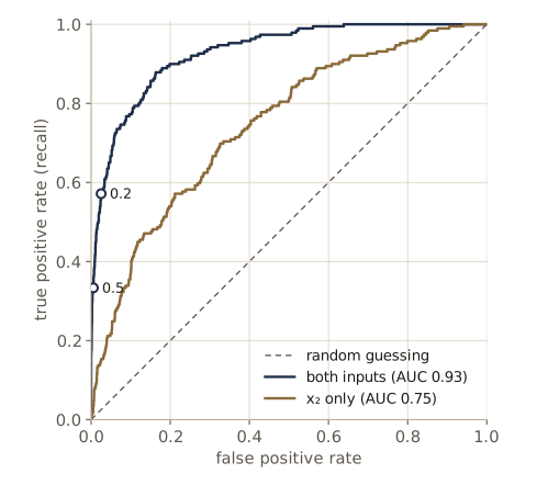
Notice that the AUC depends only on the ordering of the scores. Any increasing function of the score, for instance the logit instead of the probability, gives the same curve and area, so a model can have an excellent AUC and badly calibrated probabilities. ROC curves extend to more than two classes (one curve per class against the rest, for instance), but the picture quickly becomes unwieldy.
In practice. For rare positives, report precision and recall at the operating point you intend to use, not only accuracy or AUC. The AUC averages over thresholds nobody will use, and at a 4% prior a small false positive rate can still mean that most flagged cases are false alarms.
Generative classifiers
We now build posteriors from models of the data. For two classes, Bayes’ theorem can be rewritten as
\[p(\mathcal{C}_1 \mid \mathbf{x}) = \frac{p(\mathbf{x} \mid \mathcal{C}_1)p(\mathcal{C}_1)}{p(\mathbf{x} \mid \mathcal{C}_1)p(\mathcal{C}_1) + p(\mathbf{x} \mid \mathcal{C}_2)p(\mathcal{C}_2)} = \frac{1}{1 + \exp(-a)} = \sigma(a), \qquad a = \ln\frac{p(\mathbf{x} \mid \mathcal{C}_1)p(\mathcal{C}_1)}{p(\mathbf{x} \mid \mathcal{C}_2)p(\mathcal{C}_2)}.\]The logistic sigmoid \(\sigma(a) = 1/(1 + e^{-a})\) squashes the real line into \((0, 1)\) and satisfies \(\sigma(-a) = 1 - \sigma(a)\). Its inverse, \(a = \ln\{\sigma/(1 - \sigma)\}\), is the logit, and here it is the log of the posterior odds, \(\ln\{p(\mathcal{C}_1 \mid \mathbf{x})/p(\mathcal{C}_2 \mid \mathbf{x})\}\). Writing the posterior this way is only a change of notation. It becomes useful when \(a(\mathbf{x})\) turns out to be a simple function, and below it will be linear.
For \(K\) classes the same rewriting gives the softmax function (also called the normalized exponential)
\[p(\mathcal{C}_k \mid \mathbf{x}) = \frac{\exp(a_k)}{\sum_j \exp(a_j)}, \qquad a_k = \ln\left\{p(\mathbf{x} \mid \mathcal{C}_k)p(\mathcal{C}_k)\right\}.\]It is a smooth version of “max”: if one \(a_k\) is much larger than all the others, its posterior is close to 1 and the rest close to 0. With \(K = 2\) it reduces to the sigmoid of \(a_1 - a_2\).
Continuous inputs
Assume Gaussian class-conditional densities that share one covariance matrix, \(p(\mathbf{x} \mid \mathcal{C}_k) = \mathcal{N}(\mathbf{x} \mid \boldsymbol{\mu}_k, \boldsymbol{\Sigma})\). For two classes, the logit is a difference of two log densities plus the log prior odds. Expanding the quadratic forms,
\[\begin{aligned} a &= -\tfrac12(\mathbf{x} - \boldsymbol{\mu}_1)^{\mathrm{T}}\boldsymbol{\Sigma}^{-1}(\mathbf{x} - \boldsymbol{\mu}_1) + \tfrac12(\mathbf{x} - \boldsymbol{\mu}_2)^{\mathrm{T}}\boldsymbol{\Sigma}^{-1}(\mathbf{x} - \boldsymbol{\mu}_2) + \ln\frac{p(\mathcal{C}_1)}{p(\mathcal{C}_2)} \\ &= (\boldsymbol{\mu}_1 - \boldsymbol{\mu}_2)^{\mathrm{T}}\boldsymbol{\Sigma}^{-1}\mathbf{x} - \tfrac12\boldsymbol{\mu}_1^{\mathrm{T}}\boldsymbol{\Sigma}^{-1}\boldsymbol{\mu}_1 + \tfrac12\boldsymbol{\mu}_2^{\mathrm{T}}\boldsymbol{\Sigma}^{-1}\boldsymbol{\mu}_2 + \ln\frac{p(\mathcal{C}_1)}{p(\mathcal{C}_2)}. \end{aligned}\]The normalization constants cancel because the covariance is shared, and so do the terms \(\mathbf{x}^{\mathrm{T}}\boldsymbol{\Sigma}^{-1}\mathbf{x}\). What remains is linear in \(\mathbf{x}\):
Result. With shared-covariance Gaussian classes, \(p(\mathcal{C}_1 \mid \mathbf{x}) = \sigma(\mathbf{w}^{\mathrm{T}}\mathbf{x} + w_0)\) with
\[\mathbf{w} = \boldsymbol{\Sigma}^{-1}(\boldsymbol{\mu}_1 - \boldsymbol{\mu}_2), \qquad w_0 = -\tfrac12\boldsymbol{\mu}_1^{\mathrm{T}}\boldsymbol{\Sigma}^{-1}\boldsymbol{\mu}_1 + \tfrac12\boldsymbol{\mu}_2^{\mathrm{T}}\boldsymbol{\Sigma}^{-1}\boldsymbol{\mu}_2 + \ln\frac{p(\mathcal{C}_1)}{p(\mathcal{C}_2)}.\]For \(K\) classes, \(p(\mathcal{C}_k \mid \mathbf{x})\) is the softmax of \(a_k = \mathbf{w}_k^{\mathrm{T}}\mathbf{x} + w_{k0}\) with \(\mathbf{w}_k = \boldsymbol{\Sigma}^{-1}\boldsymbol{\mu}_k\) and \(w_{k0} = -\tfrac12\boldsymbol{\mu}_k^{\mathrm{T}}\boldsymbol{\Sigma}^{-1}\boldsymbol{\mu}_k + \ln p(\mathcal{C}_k)\).
The posterior is a single-layer network with a sigmoid or softmax output: exactly the form we will later fit directly. The priors enter only through the biases, so changing them shifts the decision boundary parallel to itself. If each class has its own covariance \(\boldsymbol{\Sigma}_k\), the quadratic terms no longer cancel and the boundaries become quadratic surfaces (a quadratic discriminant).
We check the result by computing the posterior two ways: from Bayes’ theorem with the densities evaluated by scipy.stats, and from the sigmoid of the linear function.
mu_a, mu_b = np.array([1.0, 0.5]), np.array([-0.5, -1.0])
Sigma_ab = np.array([[1.0, 0.6], [0.6, 2.0]])
p_a = 0.3                                                      # p(C1)

Si_mu_a, Si_mu_b = np.linalg.solve(Sigma_ab, mu_a), np.linalg.solve(Sigma_ab, mu_b)
w_gen = Si_mu_a - Si_mu_b                                      # Sigma^-1 (mu_1 - mu_2)
w0_gen = -0.5 * mu_a @ Si_mu_a + 0.5 * mu_b @ Si_mu_b + np.log(p_a / (1 - p_a))

X_q = 2.0 * rng.normal(size=(5, 2))
log_j1 = stats.multivariate_normal(mu_a, Sigma_ab).logpdf(X_q) + np.log(p_a)
log_j2 = stats.multivariate_normal(mu_b, Sigma_ab).logpdf(X_q) + np.log(1 - p_a)
print("Bayes' theorem:  ", np.exp(log_j1 - np.logaddexp(log_j1, log_j2)))
print("sigma(w^T x + w0):", expit(X_q @ w_gen + w0_gen))
Bayes' theorem:   [0.4907 0.0275 0.856  0.3463 0.3045]
sigma(w^T x + w0): [0.4907 0.0275 0.856  0.3463 0.3045]
Maximum likelihood solution
In practice the means, covariance, and priors are unknown and we fit them by maximum likelihood from labeled data. For two classes with \(t_n = 1\) for \(\mathcal{C}_1\) and prior \(p(\mathcal{C}_1) = \pi\), the likelihood is
\[p(\mathbf{t}, \mathbf{X} \mid \pi, \boldsymbol{\mu}_1, \boldsymbol{\mu}_2, \boldsymbol{\Sigma}) = \prod_{n=1}^{N}\left[\pi\,\mathcal{N}(\mathbf{x}_n \mid \boldsymbol{\mu}_1, \boldsymbol{\Sigma})\right]^{t_n}\left[(1 - \pi)\,\mathcal{N}(\mathbf{x}_n \mid \boldsymbol{\mu}_2, \boldsymbol{\Sigma})\right]^{1 - t_n}.\]Its logarithm splits into separate groups of terms for each parameter, and each group is a problem we have solved before. The terms in \(\pi\) are \(\sum_n\{t_n\ln\pi + (1 - t_n)\ln(1 - \pi)\}\), a Bernoulli log likelihood, maximized by \(\pi = N_1/N\), the fraction of training points in \(\mathcal{C}_1\). The terms in \(\boldsymbol{\mu}_1\) are a Gaussian log likelihood over the points of \(\mathcal{C}_1\) only, so \(\boldsymbol{\mu}_1 = \frac{1}{N_1}\sum_n t_n\mathbf{x}_n\), the class mean; likewise for \(\boldsymbol{\mu}_2\). The terms in \(\boldsymbol{\Sigma}\) collect to \(-\frac{N}{2}\ln\lvert\boldsymbol{\Sigma}\rvert - \frac{N}{2}\operatorname{Tr}(\boldsymbol{\Sigma}^{-1}\mathbf{S})\), which the standard Gaussian result maximizes at \(\boldsymbol{\Sigma} = \mathbf{S}\), with
\[\mathbf{S} = \sum_k \frac{N_k}{N}\mathbf{S}_k, \qquad \mathbf{S}_k = \frac{1}{N_k}\sum_{n \in \mathcal{C}_k}(\mathbf{x}_n - \boldsymbol{\mu}_k)(\mathbf{x}_n - \boldsymbol{\mu}_k)^{\mathrm{T}},\]the within-class covariances averaged with weights equal to the class fractions. The same results hold for \(K\) classes (Bishop & Bishop exercises 5.13–5.14; the full derivation is in Intro to ML, module 04). The fitting code is short, and converting the fitted Gaussians into the weights of a softmax layer is one more function.
def fit_shared_gaussian(X, labels, K):
    """ML priors N_k/N, class means, and the pooled covariance S."""
    priors = np.bincount(labels, minlength=K) / len(X)
    means = np.array([X[labels == k].mean(axis=0) for k in range(K)])
    R = X - means[labels]                          # x_n - mu_k for each point's class
    return priors, means, R.T @ R / len(X)         # S = sum_k (N_k / N) S_k

def gaussian_to_layer(priors, means, Sigma):
    """Columns (w_k0, w_k) with w_k = Sigma^-1 mu_k, w_k0 = -mu_k^T Sigma^-1 mu_k / 2 + ln p(C_k)."""
    Si_mu = np.linalg.solve(Sigma, means.T)                          # (D, K)
    w0 = -0.5 * np.sum(means.T * Si_mu, axis=0) + np.log(priors)
    return np.vstack([w0, Si_mu])                                    # (D + 1, K)

def log_softmax(A):
    """ln y_k = a_k - ln sum_j exp(a_j), row by row, without overflow."""
    return A - logsumexp(A, axis=1, keepdims=True)

def softmax(A):
    return np.exp(log_softmax(A))

rng_g = np.random.default_rng(58)
mus_g = np.array([[0.0, 2.0], [2.0, -1.0], [-2.0, -1.0]])
Sigma_g = np.array([[1.0, 0.5], [0.5, 1.5]])
N_g = [150, 60, 90]
X_g = np.vstack([rng_g.multivariate_normal(m, Sigma_g, size=n) for m, n in zip(mus_g, N_g)])
lab_g = np.repeat(np.arange(3), N_g)

pri_g, mu_g, S_g = fit_shared_gaussian(X_g, lab_g, 3)
print("priors:", pri_g, "\nmeans:\n", mu_g, "\npooled covariance:\n", S_g)
W_g = gaussian_to_layer(pri_g, mu_g, S_g)
P_layer = softmax(add_bias(X_g) @ W_g)
log_joint = np.column_stack([stats.multivariate_normal(mu_g[k], S_g).logpdf(X_g)
                             + np.log(pri_g[k]) for k in range(3)])
P_bayes = np.exp(log_joint - logsumexp(log_joint, axis=1, keepdims=True))
print(f"softmax layer vs Bayes' theorem: max difference {np.abs(P_layer - P_bayes).max():.1e}")
print(f"training accuracy {np.mean(P_layer.argmax(axis=1) == lab_g):.3f}")
priors: [0.5 0.2 0.3]
means:
 [[ 0.0371  2.0344]
 [ 1.8124 -1.1404]
 [-1.9664 -1.0247]]
pooled covariance:
 [[1.1092 0.5255]
 [0.5255 1.4332]]
softmax layer vs Bayes' theorem: max difference 6.7e-16
training accuracy 0.910
The estimates are close to the generating values (priors 0.5, 0.2, 0.3; covariance entries 1, 0.5, 1.5), and the fitted Gaussians turn into a softmax layer with the same posteriors as Bayes’ theorem. Note that log_softmax uses the log-sum-exp trick, which we will need again for training.
Two cautions about this approach. Maximum likelihood for a Gaussian is not robust, so a few outlying points can drag a class mean and inflate the covariance, just as they dragged least squares. And the number of parameters grows quickly: in \(M\) dimensions we fit \(2M\) mean values, \(M(M+1)/2\) covariance entries, and a prior, \(M(M+5)/2 + 1\) in all, while the posterior it produces has only \(M + 1\) parameters.
for M in [2, 10, 100, 784]:
    print(f"M = {M:4d}: generative {M * (M + 5) // 2 + 1:7d} parameters,  "
          f"logistic regression {M + 1:4d}")
M =    2: generative       8 parameters,  logistic regression    3
M =   10: generative      76 parameters,  logistic regression   11
M =  100: generative    5251 parameters,  logistic regression  101
M =  784: generative  309289 parameters,  logistic regression  785
For a 28 by 28 image, the generative model estimates over three hundred thousand numbers to produce a posterior that is determined by 785. That imbalance is the main argument for fitting the posterior directly.
Discrete features
Now let the inputs be binary, \(x_i \in \{0, 1\}\), such as the presence of words in a message or of flags in a log entry. A general distribution over \(D\) binary features needs \(2^D - 1\) numbers per class, which is hopeless beyond a few dozen features. The naive Bayes assumption treats the features as independent given the class:
\[p(\mathbf{x} \mid \mathcal{C}_k) = \prod_{i=1}^{D}\mu_{ki}^{x_i}(1 - \mu_{ki})^{1 - x_i},\]with one parameter \(\mu_{ki} = p(x_i = 1 \mid \mathcal{C}_k)\) per class and feature. Then
\[a_k(\mathbf{x}) = \ln\left\{p(\mathbf{x} \mid \mathcal{C}_k)p(\mathcal{C}_k)\right\} = \sum_{i=1}^{D}\left\{x_i\ln\mu_{ki} + (1 - x_i)\ln(1 - \mu_{ki})\right\} + \ln p(\mathcal{C}_k),\]which is again linear in the inputs: weights \(\ln\{\mu_{ki}/(1 - \mu_{ki})\}\) and bias \(\sum_i\ln(1 - \mu_{ki}) + \ln p(\mathcal{C}_k)\). The posterior is once more a softmax layer. Maximum likelihood sets \(\mu_{ki}\) to the fraction of class-\(k\) examples with \(x_i = 1\) (Bishop & Bishop exercise 5.15). With few examples, a fraction of exactly 0 or 1 would make a log infinite; the usual fix adds one pseudo-count to each outcome, which is what we do here. Features with \(L > 2\) states work the same way with a 1-of-\(L\) coding of each feature.
rng_nb = np.random.default_rng(59)
K_nb, D_nb, n_per = 3, 8, 200
mu_nb_true = rng_nb.uniform(0.1, 0.9, size=(K_nb, D_nb))           # p(x_i = 1 | C_k)
lab_nb = np.repeat(np.arange(K_nb), n_per)
X_nb = (rng_nb.random((K_nb * n_per, D_nb)) < mu_nb_true[lab_nb]).astype(float)

counts = np.array([X_nb[lab_nb == k].sum(axis=0) for k in range(K_nb)])
mu_nb = (counts + 1) / (n_per + 2)                                  # fractions, plus one pseudo-count
pri_nb = np.bincount(lab_nb) / len(lab_nb)
W_nb = np.vstack([np.log(1 - mu_nb).sum(axis=1) + np.log(pri_nb),   # biases
                  (np.log(mu_nb) - np.log(1 - mu_nb)).T])           # (D + 1, K)

x_new = X_nb[:4]
direct = np.array([[np.prod(mu_nb[k] ** x * (1 - mu_nb[k]) ** (1 - x)) * pri_nb[k]
                    for k in range(K_nb)] for x in x_new])
direct /= direct.sum(axis=1, keepdims=True)
print(f"product formula vs softmax layer: max difference "
      f"{np.abs(direct - softmax(add_bias(x_new) @ W_nb)).max():.1e}")
print(f"largest error in the estimated mu_ki: {np.abs(mu_nb - mu_nb_true).max():.3f}")
print(f"training accuracy {np.mean((add_bias(X_nb) @ W_nb).argmax(axis=1) == lab_nb):.3f}")
product formula vs softmax layer: max difference 2.5e-16
largest error in the estimated mu_ki: 0.047
training accuracy 0.797
Exponential family
The Gaussian and the Bernoulli cases are two instances of one result. Suppose each class-conditional density belongs to the exponential family (module 03) in the restricted form
\[p(\mathbf{x} \mid \boldsymbol{\lambda}_k, s) = \frac{1}{s}\,h\!\left(\frac{\mathbf{x}}{s}\right)g(\boldsymbol{\lambda}_k)\exp\left\{\frac{1}{s}\boldsymbol{\lambda}_k^{\mathrm{T}}\mathbf{x}\right\},\]where the natural parameters \(\boldsymbol{\lambda}_k\) differ between classes and the scale \(s\) is shared. Then \(h\) is common to all classes and cancels from every posterior, and
\[a_k(\mathbf{x}) = \frac{1}{s}\boldsymbol{\lambda}_k^{\mathrm{T}}\mathbf{x} + \ln g(\boldsymbol{\lambda}_k) + \ln p(\mathcal{C}_k),\]again linear in \(\mathbf{x}\). For two classes, \(a = a_1 - a_2\) and the posterior is a sigmoid of a linear function. So for a whole family of class-conditional densities, the posterior is a single layer with a sigmoid or softmax output. Densities outside this family, a mixture of Gaussians for one class for instance, give other shapes, and that is one motivation for the discriminative approach.
Discriminative classifiers
The generative route produced posteriors of the form “sigmoid or softmax of a linear function”, with the weights computed indirectly from fitted densities. The discriminative route takes that form as the model and fits its weights directly, by maximizing the likelihood of the labels given the inputs, \(\prod_n p(t_n \mid \mathbf{x}_n)\). It spends no parameters on the distribution of the inputs, and it does not suffer when the assumed densities are wrong, which they usually are. This is how neural networks classify.
Activation functions
Regression used \(y(\mathbf{x}, \mathbf{w}) = \mathbf{w}^{\mathrm{T}}\mathbf{x} + w_0\), which ranges over the whole real line. To output probabilities we pass the linear function through a fixed nonlinearity,
\[y(\mathbf{x}, \mathbf{w}) = f\left(\mathbf{w}^{\mathrm{T}}\mathbf{x} + w_0\right).\]In machine learning \(f\) is the activation function; in statistics its inverse \(f^{-1}\) is the link function. A surface of constant \(y\) is a surface of constant \(\mathbf{w}^{\mathrm{T}}\mathbf{x} + w_0\), which is a hyperplane, so the decision boundaries stay linear even though \(f\) is not. Models of this form are generalized linear models. Because \(f\) is nonlinear, the output is not a linear function of \(\mathbf{w}\) and there is no closed-form fit, but these models remain far simpler than the multilayer networks of module 06.
Fixed basis functions
Everything in this module works equally well on a fixed nonlinear transformation of the inputs, a feature vector \(\boldsymbol{\phi}(\mathbf{x})\) with \(M\) components, one of which is the constant \(\phi_0 = 1\) that carries the bias. A hyperplane in feature space is then a curved boundary in input space, and classes that no hyperplane separates in \(\mathbf{x}\) may be separable in \(\boldsymbol{\phi}\). From here on we write every model in terms of \(\boldsymbol{\phi}\).
Our example has one class clustered around the origin and the other on a ring around it. No line in the plane separates them: both class means sit near the origin. The squared coordinates \(\phi_1 = x_1^2\) and \(\phi_2 = x_2^2\) turn the ring into a band far from the origin of feature space and the cluster into a corner near it, so that a line \(\phi_1 + \phi_2 = \text{const}\), a circle in the original plane, separates them.
rng_ring = np.random.default_rng(57)
n_ring = 150
X_in = rng_ring.normal(0.0, 0.6, size=(n_ring, 2))                   # C1 (t = 1): a cluster
angle = rng_ring.uniform(0.0, 2 * np.pi, n_ring)
radius = rng_ring.normal(2.0, 0.35, n_ring)
X_out = np.column_stack([radius * np.cos(angle), radius * np.sin(angle)])  # C2 (t = 0): a ring
X_r = np.vstack([X_in, X_out])
t_r = np.r_[np.ones(n_ring), np.zeros(n_ring)]

def ring_features(X):
    """phi(x) = (1, x1^2, x2^2)."""
    return np.column_stack([np.ones(len(X)), X[:, 0] ** 2, X[:, 1] ** 2])

print("class means in x:  ", X_in.mean(axis=0), X_out.mean(axis=0))
print("class means in phi:", ring_features(X_in).mean(axis=0)[1:],
      ring_features(X_out).mean(axis=0)[1:])
class means in x:   [-0.0291 -0.0118] [-0.1732  0.0089]
class means in phi: [0.2881 0.3155] [1.9834 2.0015]
Features cannot remove overlap that is really there. If the class-conditional densities overlap in \(\mathbf{x}\), the true posterior is strictly between 0 and 1 in that region, and no transformation changes this; a poor transformation can even create overlap. What good features do is make the posterior easy to model. The weakness of fixed features is that someone has to choose them, and the number needed grows quickly with the input dimension; module 06 removes that weakness by learning the features.
Logistic regression
For two classes the discriminative model is
\[p(\mathcal{C}_1 \mid \boldsymbol{\phi}) = y(\boldsymbol{\phi}) = \sigma\left(\mathbf{w}^{\mathrm{T}}\boldsymbol{\phi}\right), \qquad p(\mathcal{C}_2 \mid \boldsymbol{\phi}) = 1 - y(\boldsymbol{\phi}).\]Statisticians call it logistic regression, although it classifies. As a network it is one layer: \(M\) inputs \(\phi_i\), one weight each, a sigmoid output unit. It has \(M\) parameters, one per feature, where the generative model needed a number that grows like \(M^2/2\).
The error function. Each label is a Bernoulli draw with probability \(y_n = \sigma(a_n)\), \(a_n = \mathbf{w}^{\mathrm{T}}\boldsymbol{\phi}_n\), so the likelihood is \(\prod_n y_n^{t_n}(1 - y_n)^{1 - t_n}\), and its negative logarithm is the cross-entropy error function
\[E(\mathbf{w}) = -\sum_{n=1}^{N}\left\{t_n\ln y_n + (1 - t_n)\ln(1 - y_n)\right\}.\]The gradient. The sigmoid’s derivative is \(d\sigma/da = \sigma(1 - \sigma)\), which follows from differentiating \((1 + e^{-a})^{-1}\). By the chain rule, the derivative of one term with respect to its pre-activation is
\[\frac{\partial E_n}{\partial a_n} = -\frac{t_n}{y_n}\,y_n(1 - y_n) + \frac{1 - t_n}{1 - y_n}\,y_n(1 - y_n) = -t_n(1 - y_n) + (1 - t_n)\,y_n = y_n - t_n,\]and since \(\partial a_n/\partial\mathbf{w} = \boldsymbol{\phi}_n\),
Result. For logistic regression with the cross-entropy error, \(\nabla E(\mathbf{w}) = \sum_{n=1}^{N}(y_n - t_n)\boldsymbol{\phi}_n\). The sigmoid’s derivative cancels, and each point contributes its error \(y_n - t_n\) times its feature vector, the same form as the sum-of-squares gradient of linear regression in module 04.
For the code, note that \(\ln y = a - \ln(1 + e^{a})\) and \(\ln(1 - y) = -\ln(1 + e^{a})\), so each term of the error is \(\ln(1 + e^{a_n}) - t_n a_n\). np.logaddexp(0, a) computes \(\ln(1 + e^{a})\) without overflow, and we never take the logarithm of a probability that has rounded to zero. We check the gradient against central finite differences before trusting it; every hand-derived gradient in this course gets the same check.
def cross_entropy(w, Phi, t):
    """E(w) = sum_n ln(1 + e^{a_n}) - t_n a_n, the stable form of the cross-entropy."""
    a = Phi @ w
    return np.sum(np.logaddexp(0.0, a) - t * a)

def cross_entropy_grad(w, Phi, t):
    return Phi.T @ (expit(Phi @ w) - t)                 # sum_n (y_n - t_n) phi_n

def numerical_gradient(f, w, h=1e-6):
    """Central differences, one parameter at a time; works for any array shape."""
    g = np.zeros_like(w)
    for i in np.ndindex(w.shape):
        e = np.zeros_like(w)
        e[i] = h
        g[i] = (f(w + e) - f(w - e)) / (2 * h)
    return g

Phi_r = ring_features(X_r)
w_test = rng.normal(size=3)
g_exact = cross_entropy_grad(w_test, Phi_r, t_r)
g_fd = numerical_gradient(lambda v: cross_entropy(v, Phi_r, t_r), w_test)
print("analytic gradient:", g_exact)
print(f"relative difference from finite differences: "
      f"{np.linalg.norm(g_exact - g_fd) / np.linalg.norm(g_fd):.1e}")
analytic gradient: [ 37.6417 227.884   55.5132]
relative difference from finite differences: 1.8e-10
Training. Setting \(\nabla E = 0\) gives no closed form, because \(y_n\) depends nonlinearly on \(\mathbf{w}\). The error is convex, though (its Hessian \(\sum_n y_n(1 - y_n)\boldsymbol{\phi}_n\boldsymbol{\phi}_n^{\mathrm{T}}\) is positive semidefinite), so any local minimum is global and plain gradient descent finds it. We divide the gradient by \(N\) so that the learning rate does not depend on the size of the data set, and fit the model twice: on the raw inputs \((1, x_1, x_2)\) and on the ring features.
def gradient_descent(grad, w, eta, n_steps, error=None, report=()):
    """w <- w - eta * grad(w); prints error(w) at the listed steps."""
    for step in range(1, n_steps + 1):
        w = w - eta * grad(w)
        if step in report:
            print(f"  step {step:5d}: E/N = {error(w):.4f}")
    return w

N_r = len(t_r)
fits = {}
for name, Phi_f in [("raw inputs", add_bias(X_r)), ("ring features", Phi_r)]:
    print(name)
    fits[name] = gradient_descent(
        lambda v: cross_entropy_grad(v, Phi_f, t_r) / N_r, np.zeros(Phi_f.shape[1]), eta=0.5,
        n_steps=3000, error=lambda v: cross_entropy(v, Phi_f, t_r) / N_r,
        report=(1, 10, 100, 1000, 3000))
    acc = np.mean((Phi_f @ fits[name] > 0) == t_r)
    print(f"  w = {fits[name]},  training accuracy {acc:.3f}")
raw inputs
  step     1: E/N = 0.6925
  step    10: E/N = 0.6909
  step   100: E/N = 0.6908
  step  1000: E/N = 0.6908
  step  3000: E/N = 0.6908
  w = [ 0.0129  0.128  -0.0129],  training accuracy 0.533
ring features
  step     1: E/N = 0.5636
  step    10: E/N = 0.3847
  step   100: E/N = 0.1637
  step  1000: E/N = 0.1310
  step  3000: E/N = 0.1308
  w = [ 5.5324 -3.1045 -2.7177],  training accuracy 0.953
On the raw inputs the model can do no better than a line through a disc and a ring, and its error stays near \(\ln 2 \approx 0.693\) per point, the value for predicting one half everywhere. On the ring features the error falls steadily and 95% of the points are classified correctly; the rest lie where the cluster’s tail meets the inner edge of the ring, a genuine overlap. The learned boundary \(w_0 + w_1x_1^2 + w_2x_2^2 = 0\) is an ellipse close to a circle, because \(w_1\) and \(w_2\) are similar.
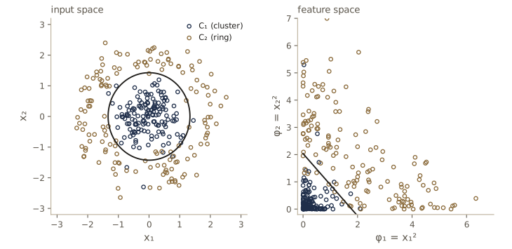
Gradient descent needed thousands of steps here. Because the error is convex and close to quadratic, Newton’s method converges in a handful of steps; for logistic regression it takes the form of a sequence of weighted least-squares problems, called iterative reweighted least squares (IRLS), derived and implemented in Intro to ML, module 04. IRLS needs the \(M \times M\) Hessian, which is fine for three weights and out of the question for the millions of weights in a deep network, so from module 07 on we train with (stochastic) gradient descent and its relatives.
Watch out. If the training data are linearly separable (in feature space), maximum likelihood has no finite solution. Any separating hyperplane can be scaled up: every \(a_n\) grows with the right sign, every \(y_n\) moves toward its target, and the error keeps falling toward zero as \(\lVert\mathbf{w}\rVert \to \infty\). The sigmoid becomes a step, every training point gets probability 1 for its class, and which of the many separating hyperplanes you end up with depends on the optimizer and the starting point. This happens however large \(N\) is, as long as the classes are separable. A regularizer such as \(\tfrac{\alpha}{2}\lVert\mathbf{w}\rVert^2\) removes the problem (module 09).
Generative or discriminative? Both approaches give a linear logit, so on data that really are shared-covariance Gaussians they should agree, and the generative fit, which uses more assumptions, can even be a little better with little data. When the assumptions fail, the discriminative fit is usually better. We compare them on two data sets. In the first, both classes are Gaussian with a shared covariance. In the second, 30% of class \(\mathcal{C}_2\) comes from a separate cluster far out on \(\mathcal{C}_2\)’s own side, a class that is not Gaussian at all.
def logistic_fit(X, t, eta=0.5, n_steps=4000):
    """Logistic regression on (1, x) by gradient descent from zero."""
    Phi = add_bias(X)
    return gradient_descent(lambda v: cross_entropy_grad(v, Phi, t) / len(t),
                            np.zeros(Phi.shape[1]), eta, n_steps)

def gaussian_fit_binary(X, t):
    """Shared-covariance generative classifier; returns (w0, w) for p(C1 | x) = sigma(.)."""
    pri, mu, S = fit_shared_gaussian(X, (1 - t).astype(int), 2)     # label 0 is C1 (t = 1)
    W = gaussian_to_layer(pri, mu, S)
    return W[:, 0] - W[:, 1]

def sample_gd(n, far, rng_):
    """Class C1 (t = 1) and class C2 (t = 0); with far=True, 30% of C2 is a distant cluster."""
    Sig = np.array([[1.0, 0.3], [0.3, 0.8]])
    X1 = rng_.multivariate_normal([-1.0, 0.5], Sig, size=n)
    X2 = rng_.multivariate_normal([1.0, -0.5], Sig, size=n)
    if far:
        m = int(0.3 * n)
        X2[:m] = rng_.normal([7.0, -2.0], 0.5, size=(m, 2))
    return np.vstack([X1, X2]), np.r_[np.ones(n), np.zeros(n)]

rng_gd = np.random.default_rng(60)
gd_fits = {}
for far in [False, True]:
    X_tr, t_tr = sample_gd(100, far, rng_gd)
    X_te, t_te = sample_gd(5000, far, rng_gd)
    w_gauss, w_logit = gaussian_fit_binary(X_tr, t_tr), logistic_fit(X_tr, t_tr)
    gd_fits[far] = (X_tr, t_tr, w_gauss, w_logit)
    errs = [np.mean((add_bias(X_te) @ v > 0) != t_te) for v in (w_gauss, w_logit)]
    print(f"far cluster {str(far):5s}: test error  generative {errs[0]:.3f}   "
          f"logistic regression {errs[1]:.3f}")
far cluster False: test error  generative 0.084   logistic regression 0.083
far cluster True : test error  generative 0.161   logistic regression 0.066
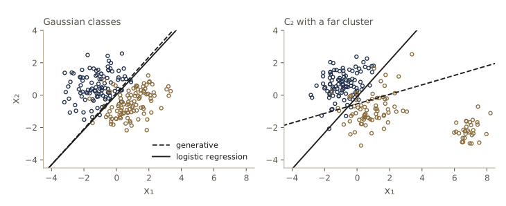
With Gaussian classes the two methods tie. With the far cluster the generative model’s mean for \(\mathcal{C}_2\) moves toward the cluster and its pooled covariance stretches, which rotates the boundary until it cuts through both main clusters (test error 0.161, against 0.066 for logistic regression); logistic regression only cares about the posterior near the boundary, where the far cluster has no influence. This is the same lack of robustness that broke least squares, now in a density model. It is also a small version of the general lesson: modeling the inputs is extra work, and extra risk, when all we need is the posterior.
Multi-class logistic regression
For \(K\) classes the model is a softmax layer,
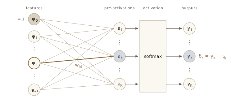
\[p(\mathcal{C}_k \mid \boldsymbol{\phi}) = y_k(\boldsymbol{\phi}) = \frac{\exp(a_k)}{\sum_{j}\exp(a_j)}, \qquad a_k = \mathbf{w}_k^{\mathrm{T}}\boldsymbol{\phi},\]usually called softmax regression or multinomial logistic regression. As a network it has \(M\) inputs, \(K\) output units, and a weight \(w_{ki}\) on each connection; we collect the \(\mathbf{w}_k\) as the columns of an \(M \times K\) matrix \(\mathbf{W}\), so that the pre-activations of all points are the rows of \(\mathbf{\Phi}\mathbf{W}\).
The softmax derivatives. Differentiating \(y_k = e^{a_k}/\sum_j e^{a_j}\) with the quotient rule gives
\[\frac{\partial y_k}{\partial a_j} = y_k\left(I_{kj} - y_j\right),\]where \(I_{kj}\) is 1 when \(k = j\) and 0 otherwise. Every output depends on every pre-activation, because they share the normalizer.
The error and its gradient. With one-hot targets \(\mathbf{t}_n\), the likelihood is \(\prod_n\prod_k y_{nk}^{t_{nk}}\), and the multi-class cross-entropy is
\[E(\mathbf{w}_1, \dots, \mathbf{w}_K) = -\sum_{n=1}^{N}\sum_{k=1}^{K}t_{nk}\ln y_{nk}.\]For one point, the derivative with respect to a pre-activation uses the softmax derivatives and \(\sum_k t_{nk} = 1\):
\[\frac{\partial E_n}{\partial a_{nj}} = -\sum_k \frac{t_{nk}}{y_{nk}}\,y_{nk}(I_{kj} - y_{nj}) = -t_{nj} + y_{nj}\sum_k t_{nk} = y_{nj} - t_{nj}.\]With \(\partial a_{nj}/\partial\mathbf{w}_j = \boldsymbol{\phi}_n\), the gradient is
Result. \(\nabla_{\mathbf{w}_j}E = \sum_{n=1}^{N}(y_{nj} - t_{nj})\boldsymbol{\phi}_n\), or for all classes at once \(\nabla_{\mathbf{W}}E = \mathbf{\Phi}^{\mathrm{T}}(\mathbf{Y} - \mathbf{T})\). For the single weight \(w_{ki}\) joining feature \(i\) to output \(k\), \(\partial E/\partial w_{ki} = \sum_n \delta_{nk}\,\phi_i(\mathbf{x}_n)\) with \(\delta_{nk} = y_{nk} - t_{nk}\).
Read the last line against the network diagram: the gradient for a weight is the value at its input end times the error at its output end. Backpropagation in module 08 computes an error \(\delta\) for every unit, hidden ones included, and then uses exactly this rule for every weight in the network; the output-layer errors it starts from are the \(y_k - t_k\) derived here.
Computing it stably. The softmax is unchanged if we add the same constant to every \(a_k\), so we subtract the largest before exponentiating. log_softmax above does this through logsumexp, and computing \(\ln y_k\) directly as \(a_k - \ln\sum_j e^{a_j}\) also avoids taking the log of an underflowed probability. Deep learning libraries do the same: their cross-entropy functions take the pre-activations (the “logits”) and never form the probabilities first.
A_big = np.array([[1000.0, 1001.0, 1002.0], [-1000.0, -1001.0, -1003.0]])
with np.errstate(over="ignore", invalid="ignore", divide="ignore"):
    naive = np.exp(A_big) / np.exp(A_big).sum(axis=1, keepdims=True)
    naive_log = np.log(naive)
print("naive softmax:\n", naive)
print("stable softmax:\n", softmax(A_big))
print("naive ln y:", naive_log[1], "  stable ln y:", log_softmax(A_big)[1])
naive softmax:
 [[nan nan nan]
 [nan nan nan]]
stable softmax:
 [[0.09   0.2447 0.6652]
 [0.7054 0.2595 0.0351]]
naive ln y: [nan nan nan]   stable ln y: [-0.349 -1.349 -3.349]
The naive version turns large pre-activations into inf/inf and small ones into 0/0; the stable version gives the right answer, including log probabilities that could not be recovered from the rounded probabilities.
Now the error, its gradient, a finite-difference check, and training on the three-class data where least squares failed.
def softmax_error(W, Phi, T):
    return -np.sum(T * log_softmax(Phi @ W))             # -sum_n sum_k t_nk ln y_nk

def softmax_grad(W, Phi, T):
    return Phi.T @ (softmax(Phi @ W) - T)                 # Phi^T (Y - T), shape (M, K)

Phi3 = add_bias(X3)
W_test = rng.normal(size=(3, 3))
G_exact = softmax_grad(W_test, Phi3, T3)
G_fd = numerical_gradient(lambda V: softmax_error(V, Phi3, T3), W_test)
print(f"relative difference from finite differences: "
      f"{np.linalg.norm(G_exact - G_fd) / np.linalg.norm(G_fd):.1e}")

W_sm3 = gradient_descent(lambda V: softmax_grad(V, Phi3, T3) / len(T3), np.zeros((3, 3)),
                         eta=0.2, n_steps=4000,
                         error=lambda V: softmax_error(V, Phi3, T3) / len(T3),
                         report=(1, 100, 1000, 4000))
pred_sm3 = (Phi3 @ W_sm3).argmax(axis=1)
print(f"training errors: softmax {np.sum(pred_sm3 != lab3)},  least squares "
      f"{np.sum(pred_ls3 != lab3)};  points per class (softmax) {np.bincount(pred_sm3)}")
shifted = softmax(Phi3 @ (W_sm3 + rng.normal(size=(3, 1))))  # add one vector to every w_k
print(f"adding the same vector to every w_k changes y by {np.abs(shifted - softmax(Phi3 @ W_sm3)).max():.1e}")
relative difference from finite differences: 2.1e-10
  step     1: E/N = 0.6328
  step   100: E/N = 0.1726
  step  1000: E/N = 0.0878
  step  4000: E/N = 0.0807
training errors: softmax 3,  least squares 56;  points per class (softmax) [59 59 62]
adding the same vector to every w_k changes y by 1.8e-15
Softmax regression separates the three classes, middle one included, with the same linear decision rule that least squares used; only the error function changed. The last line shows a redundancy: adding the same vector to every \(\mathbf{w}_k\) adds the same number to every \(a_k\) and leaves the outputs unchanged, so only differences \(\mathbf{w}_k - \mathbf{w}_j\) are determined (for \(K = 2\) this is why one sigmoid suffices). Gradient descent from zero is not bothered by this, and a weight penalty removes it.
The same comparison on the two-class data with the far points completes the picture.
for name, X, t in [("without the far points", X2, t2), ("with the far points   ", X2o, t2o)]:
    w_lr = logistic_fit(X, t)
    errors = np.sum((add_bias(X2) @ w_lr > 0) != t2)
    print(f"{name}: logistic normal at {normal_angle(w_lr):6.1f} deg, "
          f"errors on the original points {errors}")
without the far points: logistic normal at  121.1 deg, errors on the original points 6
with the far points   : logistic normal at  121.1 deg, errors on the original points 6
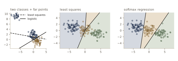
Logistic regression does not move at all to the printed precision. The cross-entropy of a point that is already classified with a wide margin is close to zero and so is its gradient, \(y_n - t_n \approx 0\): confident, correct points stop pulling on the weights. Squared error has no such off switch.
Note. Softmax regression with \(K = 2\) outputs and logistic regression with one output compute the same family of posteriors. In deep learning code you will see both: a single “logit” with a sigmoid and binary cross-entropy, or \(K\) logits with softmax cross-entropy. They are interchangeable for two classes, and only the second extends to more.
Probit regression
The logistic sigmoid came out of the generative models, but any increasing function from the real line onto \((0, 1)\) can serve as the activation, \(p(t = 1 \mid a) = f(a)\) with \(a = \mathbf{w}^{\mathrm{T}}\boldsymbol{\phi}\). One way to motivate a choice is a noisy threshold model: each input gets the label 1 if its activation \(a_n\) exceeds a random threshold \(\theta\) drawn from a density \(p(\theta)\), and 0 otherwise. Then
\[p(t = 1 \mid a) = \int_{-\infty}^{a} p(\theta)\,d\theta,\]the cumulative distribution function of the threshold. A standard Gaussian threshold gives the probit function
\[\Phi(a) = \int_{-\infty}^{a}\mathcal{N}(\theta \mid 0, 1)\,d\theta = \frac12\left\{1 + \operatorname{erf}\left(\frac{a}{\sqrt{2}}\right)\right\}, \qquad \operatorname{erf}(z) = \frac{2}{\sqrt{\pi}}\int_0^z e^{-u^2}\,du,\]where erf is the error function found in numerical libraries (unrelated to the error function \(E(\mathbf{w})\) of a model). A Gaussian threshold with another mean and variance adds nothing, since the shift and scale are absorbed into \(\mathbf{w}\). The resulting model is probit regression. Its negative log likelihood, with \(q_n = 2t_n - 1 \in \{-1, +1\}\) and the symmetry \(1 - \Phi(a) = \Phi(-a)\), is \(E(\mathbf{w}) = -\sum_n \ln\Phi(q_n a_n)\), and its gradient is
\[\nabla E(\mathbf{w}) = -\sum_{n=1}^{N} q_n\,\frac{\mathcal{N}(q_n a_n \mid 0, 1)}{\Phi(q_n a_n)}\,\boldsymbol{\phi}_n,\]which is not of the form \((y_n - t_n)\boldsymbol{\phi}_n\); we come back to this below. We use log_ndtr, which computes \(\ln\Phi\) accurately far into the tail, and fit both models to the two-class data without the far points.
def probit_error(w, Phi, t):
    return -np.sum(log_ndtr((2 * t - 1) * (Phi @ w)))

def probit_grad(w, Phi, t):
    q = 2 * t - 1
    z = q * (Phi @ w)
    ratio = np.exp(-0.5 * z**2 - 0.5 * np.log(2 * np.pi) - log_ndtr(z))   # N(z) / Phi(z)
    return -Phi.T @ (q * ratio)

def probit_fit(X, t, eta=0.5, n_steps=4000):
    Phi = add_bias(X)
    return gradient_descent(lambda v: probit_grad(v, Phi, t) / len(t),
                            np.zeros(Phi.shape[1]), eta, n_steps)

a_chk = np.linspace(-5, 5, 11)
print(f"Phi via erf vs scipy.stats.norm.cdf: {np.abs(norm_cdf(a_chk) - stats.norm.cdf(a_chk)).max():.1e}")
w_chk = rng.normal(size=3)
g_fd = numerical_gradient(lambda v: probit_error(v, add_bias(X2), t2), w_chk)
print(f"probit gradient vs finite differences: "
      f"{np.abs(probit_grad(w_chk, add_bias(X2), t2) - g_fd).max():.1e}")

w_logit2, w_probit2 = logistic_fit(X2, t2), probit_fit(X2, t2)
print("logistic w:", w_logit2, "\nprobit w:  ", w_probit2,
      "\nratio:     ", w_logit2 / w_probit2)
gap = np.abs(expit(add_bias(X2) @ w_logit2) - norm_cdf(add_bias(X2) @ w_probit2)).max()
print(f"largest difference in fitted probabilities: {gap:.3f}")
Phi via erf vs scipy.stats.norm.cdf: 1.1e-16
probit gradient vs finite differences: 2.0e-08
logistic w: [ 0.4311 -2.135   3.5409]
probit w:   [ 0.1577 -1.1161  1.9448]
ratio:      [2.7333 1.913  1.8207]
largest difference in fitted probabilities: 0.051
The fits agree once the scale is taken into account. The two slope weights of the logistic model are about 1.8 to 1.9 times those of the probit model (the ratio of the small biases is less stable), because a logistic sigmoid resembles a probit stretched horizontally. Matching the slopes at the origin gives \(\sigma(a) \approx \Phi(\lambda a)\) with \(\lambda^2 = \pi/8\), a stretch of \(1/\lambda \approx 1.6\) (exercise 7); a fit to data need not reproduce that exactly, since the curves differ away from the origin. The fitted probabilities differ by about 0.05 at most.
The difference lies in the tails. For large \(\lvert a\rvert\) the logistic sigmoid approaches 0 or 1 like \(e^{-\lvert a\rvert}\), the probit like \(e^{-a^2/2}\). A mislabeled point far on the wrong side of the boundary therefore costs about \(\lvert a\rvert\) under logistic regression but about \(a^2/2\) under probit regression, and the probit fit will work much harder to accommodate it. We add four mislabeled points, labeled \(\mathcal{C}_1\) but placed deep in \(\mathcal{C}_2\)’s territory, and refit.
X_bad = np.array([[5.0, -3.5], [5.5, -3.0], [4.5, -4.0], [5.2, -4.2]])   # labeled t = 1
X2b, t2b = np.vstack([X2, X_bad]), np.r_[t2, np.ones(4)]
for name, fit in [("logistic", logistic_fit), ("probit  ", probit_fit)]:
    w_clean, w_dirty = fit(X2, t2), fit(X2b, t2b)
    turn = normal_angle(w_dirty) - normal_angle(w_clean)
    errors = np.sum((add_bias(X2) @ w_dirty > 0) != t2)
    print(f"{name}: boundary normal turns {turn:6.1f} deg, "
          f"errors on the clean points {np.sum((add_bias(X2) @ w_clean > 0) != t2)} -> {errors}")
logistic: boundary normal turns  -18.3 deg, errors on the clean points 6 -> 9
probit  : boundary normal turns  -30.1 deg, errors on the clean points 8 -> 9
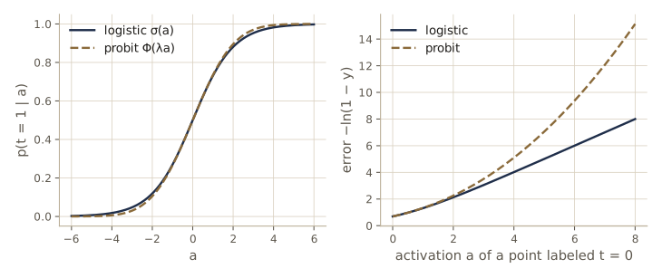
Both models are disturbed by the mislabeled points, but the probit boundary turns further, as the tail argument predicts. Logistic regression is not immune either; the far points of the least-squares experiment were harmless because they were correctly labeled. With labels that may be wrong, a standard remedy builds the flip probability into the likelihood (Intro to ML, module 04).
Canonical link functions
We have now met the gradient “error times feature”, \(\sum_n(y_n - t_n)\boldsymbol{\phi}_n\), three times: sum-of-squares with an identity output (module 04), cross-entropy with a sigmoid, and multi-class cross-entropy with a softmax. Probit regression broke the pattern. The explanation is a general property of the exponential family.
Suppose the target, rather than the input, has an exponential family distribution with natural parameter \(\eta\) and shared scale \(s\),
\[p(t \mid \eta, s) = \frac{1}{s}\,h\!\left(\frac{t}{s}\right)g(\eta)\exp\left\{\frac{\eta t}{s}\right\}.\]Differentiating the normalization condition with respect to \(\eta\) (module 03) gives the mean, \(y \equiv \mathbb{E}[t \mid \eta] = -s\,\frac{d}{d\eta}\ln g(\eta)\). That fixes a one-to-one relation between \(y\) and \(\eta\); write it \(\eta = \psi(y)\). A generalized linear model sets \(y = f(a)\) with \(a = \mathbf{w}^{\mathrm{T}}\boldsymbol{\phi}\). By the chain rule through \(\eta_n\), \(y_n\), and \(a_n\), the log likelihood has gradient
\[\begin{aligned} \nabla_{\mathbf{w}}\ln p(\mathbf{t} \mid \mathbf{w}) &= \sum_{n=1}^{N}\left\{\frac{d}{d\eta_n}\ln g(\eta_n) + \frac{t_n}{s}\right\}\frac{d\eta_n}{dy_n}\frac{dy_n}{da_n}\boldsymbol{\phi}_n \\ &= \sum_{n=1}^{N}\frac{1}{s}\left(t_n - y_n\right)\psi'(y_n)\,f'(a_n)\,\boldsymbol{\phi}_n. \end{aligned}\]Now choose the activation so that its inverse is \(\psi\), that is, \(f^{-1}(y) = \psi(y)\): the canonical link function. Then \(a_n = \eta_n\), and since \(f\) and \(\psi\) are inverse functions, \(f'(a)\,\psi'(y) = 1\). The two derivatives cancel, and the error \(E = -\ln p(\mathbf{t} \mid \mathbf{w})\) has gradient
Result. With the canonical link, \(\nabla E(\mathbf{w}) = \frac{1}{s}\sum_{n=1}^{N}(y_n - t_n)\boldsymbol{\phi}_n\). Gaussian targets: identity activation, sum-of-squares error, \(s = \beta^{-1}\) the noise variance. Bernoulli targets: logistic sigmoid, cross-entropy, \(s = 1\). Categorical targets (the vector version): softmax, multi-class cross-entropy.
The probit is a perfectly good activation for a Bernoulli target, but it is not the canonical one, so \(\psi'f' \neq 1\) and the factors do not cancel. We check all four cases numerically, comparing \((y - t)\boldsymbol{\phi}\) with a finite-difference gradient of each error.
Phi_c, t_c = add_bias(X2[:20]), t2[:20]
T_c = one_hot(rng.integers(0, 3, size=20), 3)
t_real = rng.normal(size=20)                                  # real-valued targets
w_at, W_at = rng.normal(size=3), rng.normal(size=(3, 3))

cases = [
    ("Gaussian, identity, sum of squares",
     lambda v: 0.5 * np.sum((Phi_c @ v - t_real) ** 2), w_at, Phi_c.T @ (Phi_c @ w_at - t_real)),
    ("Bernoulli, sigmoid, cross-entropy  ",
     lambda v: cross_entropy(v, Phi_c, t_c), w_at, Phi_c.T @ (expit(Phi_c @ w_at) - t_c)),
    ("categorical, softmax, cross-entropy",
     lambda V: softmax_error(V, Phi_c, T_c), W_at, Phi_c.T @ (softmax(Phi_c @ W_at) - T_c)),
    ("Bernoulli, probit, cross-entropy   ",
     lambda v: probit_error(v, Phi_c, t_c), w_at, Phi_c.T @ (norm_cdf(Phi_c @ w_at) - t_c)),
]
for name, err, where, y_minus_t in cases:
    g_fd = numerical_gradient(err, where)
    print(f"{name}: max |(y - t) phi - true gradient| = {np.abs(y_minus_t - g_fd).max():.1e}")
Gaussian, identity, sum of squares: max |(y - t) phi - true gradient| = 5.2e-09
Bernoulli, sigmoid, cross-entropy  : max |(y - t) phi - true gradient| = 4.4e-10
categorical, softmax, cross-entropy: max |(y - t) phi - true gradient| = 7.5e-09
Bernoulli, probit, cross-entropy   : max |(y - t) phi - true gradient| = 3.8e+00
The first three agree to finite-difference precision; the probit case is off by amounts of order one. The practical rule for building networks follows: pair each output activation with the negative log likelihood it is canonical for. Identity outputs go with sum-of-squares, a sigmoid with binary cross-entropy, a softmax with multi-class cross-entropy. The derivative of the error with respect to each output pre-activation is then \(y_k - t_k\), a well-scaled signal that does not vanish when the output saturates on the wrong side, and module 06 uses exactly these pairings for deep networks. (A sigmoid with a squared error, a non-canonical pairing, does vanish there; see exercise 8.)
Summary
| Method | What it models | Key equation or property |
|---|---|---|
| Linear discriminant | a label directly | \(y(\mathbf{x}) = \mathbf{w}^{\mathrm{T}}\mathbf{x} + w_0\); \(\mathbf{w}\) normal to the boundary, \(r = y/\lVert\mathbf{w}\rVert\) |
| \(K\)-class discriminant | a label directly | largest \(y_k = \mathbf{w}_k^{\mathrm{T}}\mathbf{x} + w_{k0}\); convex regions, no ambiguity |
| Least squares | posteriors, poorly | \(\widetilde{\mathbf{W}} = \widetilde{\mathbf{X}}^{\dagger}\mathbf{T}\); outputs sum to 1 but leave \([0,1]\); masking, outliers |
| Decision rules | decisions from posteriors | minimize \(\sum_k L_{kj}\,p(\mathcal{C}_k \mid \mathbf{x})\) over \(j\); reject if \(\max_k p(\mathcal{C}_k \mid \mathbf{x}) \leq \theta\) |
| Classifier measures | quality of decisions | precision, recall, F-score; ROC curve; AUC = P(positive ranked above negative) |
| Gaussian generative | \(p(\mathbf{x} \mid \mathcal{C}_k)\), \(p(\mathcal{C}_k)\) | shared \(\boldsymbol{\Sigma}\): \(\mathbf{w}_k = \boldsymbol{\Sigma}^{-1}\boldsymbol{\mu}_k\), softmax output; \(M(M+5)/2+1\) parameters |
| Naive Bayes | independent binary features | weights \(\ln\{\mu_{ki}/(1-\mu_{ki})\}\), softmax output |
| Logistic regression | \(p(\mathcal{C}_1 \mid \boldsymbol{\phi}) = \sigma(\mathbf{w}^{\mathrm{T}}\boldsymbol{\phi})\) | convex cross-entropy; \(\nabla E = \sum_n(y_n - t_n)\boldsymbol{\phi}_n\) |
| Softmax regression | \(p(\mathcal{C}_k \mid \boldsymbol{\phi})\) = softmax of \(\mathbf{w}_k^{\mathrm{T}}\boldsymbol{\phi}\) | \(\nabla_{\mathbf{W}}E = \mathbf{\Phi}^{\mathrm{T}}(\mathbf{Y} - \mathbf{T})\); compute with log-softmax |
| Probit regression | \(p(t = 1 \mid a) = \Phi(a)\) | similar fits to logistic; Gaussian tails make it less tolerant of mislabeled points |
| Canonical link | output activation matched to the likelihood | \(\partial E/\partial a_k = y_k - t_k\) |
Ideas to carry forward:
- A classifier is a network whose last layer is a sigmoid or softmax trained with cross-entropy. Everything before that layer, fixed features here and learned hidden layers from module 06 on, only changes what \(\boldsymbol{\phi}\) is.
- The gradient for a weight is the input at its tail times the error \(y_k - t_k\) at its head. Backpropagation (module 08) generalizes this rule to every layer.
- Keep inference and decision separate: learn posteriors, then choose thresholds from the losses and the priors of the deployment. Measure the result with the quantities that matter for the application, which for rare classes means precision and recall, not accuracy.
- Compute log probabilities from pre-activations with log-sum-exp, never by taking the log of a softmax output.
Exercises
- Show that for one-hot targets, \(\mathbb{E}[\mathbf{t} \mid \mathbf{x}]\) is the vector of posterior probabilities \(p(\mathcal{C}_k \mid \mathbf{x})\). Then regenerate the three-class data of
X3with 6000 points per class, fit least squares, and compare the fitted outputs with the true posteriors (which you can compute, since you know the generating Gaussians). Where is the approximation worst? - Prove that the decision regions of a \(K\)-class linear discriminant are convex, and construct a three-class data set in the plane for which the region of one class, under the optimal (Bayes) classifier, is not convex. Can softmax regression on raw inputs represent that classifier? What features would let it?
- Add a reject decision with loss \(\lambda\) to a two-class problem with loss matrix \(L_{kj}\). Derive the rule that minimizes the expected loss, show that with \(L_{kj} = 1 - I_{kj}\) it reduces to “reject when the largest posterior is below \(\theta\)”, and find \(\theta\) as a function of \(\lambda\). Check your rule on the Monte Carlo sample
x_mcby comparing its average loss with nearby thresholds. - For the part-inspection model and a threshold \(\widehat{x}\), write the four fractions \(N_{\mathrm{TP}}/N\), \(N_{\mathrm{FP}}/N\), \(N_{\mathrm{TN}}/N\), \(N_{\mathrm{FN}}/N\) as integrals of the joint densities and evaluate them with
norm_cdf. Compare with the counts in the Monte Carlo sample for \(\widehat{x} = 1\) and \(\widehat{x} = 2\). - Prove that the trapezoid area under the ROC curve equals the pairwise definition of the AUC, ties included. (Hint: consider how each positive contributes to the area as the curve moves right past the negatives.) Then show that
roc_curveis unchanged by any strictly increasing transformation of the scores and check it numerically with the logit ofscore_s. - Derive the maximum likelihood estimates of the priors, means, and shared covariance for \(K\) Gaussian classes, and check
fit_shared_gaussianagainstscipy.stats.multivariate_normalby showing numerically that small perturbations of the fitted parameters lower the log likelihood. - Show that \(\sigma'(0) = 1/4\) and that matching the slope of \(\Phi(\lambda a)\) at the origin gives \(\lambda^2 = \pi/8\). Plot \(\sigma(a) - \Phi(\lambda a)\) and find the largest difference. Repeat the mislabeled-point experiment with 1, 2, 4, and 8 bad points and plot the rotation of each boundary against the number of bad points.
- For a sigmoid output with a sum-of-squares error, show that \(\partial E_n/\partial a_n = (y_n - t_n)\,y_n(1 - y_n)\). Train logistic regression on the ring features with this error and with the cross-entropy, both from a start where every point is confidently misclassified (for instance \(\mathbf{w} = -10\,\mathbf{w}_{\text{fit}}\)), and compare how fast the error falls.
- Implement Newton’s method for logistic regression, \(\mathbf{w} \leftarrow \mathbf{w} - \mathbf{H}^{-1}\nabla E\) with \(\mathbf{H} = \mathbf{\Phi}^{\mathrm{T}}\mathbf{R}\mathbf{\Phi}\) and \(R_{nn} = y_n(1 - y_n)\), using
np.linalg.solve. How many steps does it need on the ring features to match 3000 steps of gradient descent? Then make the ring data separable (shrink the cluster) and watch \(\lVert\mathbf{w}\rVert\) over the iterations, with and without a penalty \(\tfrac{\alpha}{2}\lVert\mathbf{w}\rVert^2\). - For a Poisson target with mean \(y = e^{a}\), show that the log link is canonical and that the gradient of the negative log likelihood is \(\sum_n(y_n - t_n)\boldsymbol{\phi}_n\). Generate Poisson counts from a known weight vector, fit it by gradient descent, and check the gradient with
numerical_gradient. - In your own words: why do logistic and softmax regression give gradients of the form “output error times input”, what would go wrong if you paired a softmax output with a squared error in a deep classifier, and why is this pairing the right starting point for backpropagation?
Going further
- Bishop & Bishop, Deep Learning: Foundations and Concepts, chapter 5 — the source for this module. Exercises 5.2 (convex hulls and separability), 5.3–5.4 (linear constraints in least squares), 5.6 (a bound on the misclassification rate), 5.10 (the reject option with a loss matrix), 5.13–5.17 (generative and naive Bayes maximum likelihood), 5.20 (separable data), 5.21–5.22 (softmax derivatives), and 5.24 (the probit scaling) extend the material here.
- Intro to ML, module 04 — the same models with Fisher’s discriminant, the perceptron, IRLS, the Laplace approximation, and Bayesian logistic regression; Intro to ML, module 01 for decision theory with another example.
- Tom Fawcett, “An introduction to ROC analysis”, Pattern Recognition Letters, 2006 — a practical guide to ROC curves, AUC, and their pitfalls.
- John A. Nelder and Robert W. M. Wedderburn, “Generalized linear models”, Journal of the Royal Statistical Society, Series A, 1972 — the paper that introduced generalized linear models and canonical links.
- Andrew Y. Ng and Michael I. Jordan, “On discriminative vs. generative classifiers: a comparison of logistic regression and naive Bayes”, Advances in Neural Information Processing Systems 14, 2002 — when each approach wins, as a function of the amount of data.
- In this course: module 06 replaces the fixed features with learned ones, and module 08 propagates the output errors \(y_k - t_k\) back through the network.
These notes follow the chapters of C. M. Bishop and H. Bishop, Deep Learning: Foundations and Concepts (Springer, 2024), the course text, which the authors make free to read online. The explanations, code, figures, and exercises here are written for this course; the book remains the reference, with the full derivations and many more exercises.