CSE 676 · Module 03 · Week 2
Standard Distributions
Bernoulli, binomial, and multinomial; the multivariate Gaussian with its conditionals, marginals, and mixtures; periodic variables; the exponential family; histograms, kernels, and nearest neighbors.
Companion reading: Bishop & Bishop, Deep Learning: Foundations and Concepts, chapter 3, “Standard Distributions”
By the end of this module you can
- Fit Bernoulli and multinomial models by maximum likelihood, and explain why a network’s sigmoid and softmax outputs with a cross-entropy loss are these same likelihoods written in terms of logits.
- Describe a multivariate Gaussian through the eigenvectors and eigenvalues of its covariance, compute Mahalanobis distances and log densities stably with a Cholesky factor, and count the parameters of full, diagonal, and isotropic models.
- State the conditional and marginal distributions of a partitioned Gaussian and the linear-Gaussian version of Bayes’ theorem, and check them with exact linear algebra and with samples.
- Estimate a Gaussian by maximum likelihood, explain the bias of the covariance estimate, and update a mean one observation at a time with a 1/N or a constant step.
- Evaluate a Gaussian mixture density and its responsibilities with log-sum-exp, and fit a small mixture by gradient ascent in the same unconstrained parameters a mixture density network uses.
- Average angles correctly, and fit a von Mises distribution by maximum likelihood.
- Write the Bernoulli, categorical, and Gaussian distributions in exponential-family form, and show that maximum likelihood there is moment matching with a concave log-likelihood.
- Build histogram, kernel, and nearest-neighbor density estimates, choose their smoothing parameter, and explain why these methods scale poorly with dimension.
Contents
- Discrete variables
- The multivariate Gaussian
- Periodic variables
- The exponential family
- Nonparametric methods
- Summary
- Exercises
- Going further
Module 02 set up the rules of probability, densities, the one-dimensional Gaussian, and maximum likelihood. This module fills in the catalog: the handful of distributions that deep learning uses again and again, with their properties and their maximum likelihood fits. Each has a direct job inside a network. The Bernoulli distribution is what a sigmoid output unit predicts, the categorical distribution is what a softmax layer predicts, and a Gaussian with a network-computed mean is the probabilistic model behind a regression loss. Mixtures of Gaussians become mixture density networks in module 06 and the simplest latent-variable model in module 15. The exponential family explains why these output units pair so neatly with their losses, the story of canonical link functions in module 05.
The common task is density estimation: given observations \(\mathbf{x}_1, \dots, \mathbf{x}_N\), assumed independent and identically distributed (i.i.d.), build a model of the distribution \(p(\mathbf{x})\) that produced them. The task is ill-posed. Any density that is positive at the observed points could have generated them, so choosing a model is a model-selection question, the same one that polynomial degree raised in module 01. We take two routes. Parametric models fix a functional form with a few adjustable parameters and fit them, mostly by maximum likelihood. Nonparametric models (histograms, kernels, nearest neighbors) let the form follow the data, at the price of keeping the whole data set around. Deep learning sits between the two: a network has a fixed, large number of parameters and can still represent very flexible distributions.
The same material appears at greater length in Intro to ML, module 02, which also covers the Bayesian side (beta and Dirichlet priors, Bayesian inference for the Gaussian, Student’s t). Here we state each result, sketch the key steps, check it in code, and point to that module for the full derivations. Everything is NumPy, with SciPy used for special functions and for checking our own code.
import numpy as np
from scipy.special import expit, logsumexp, gammaln, i0e, i1e
from scipy import stats          # used only to check our own code

np.set_printoptions(precision=4, suppress=True)
rng = np.random.default_rng(3)
Discrete variables
The Bernoulli distribution
A binary variable \(x \in \{0, 1\}\) (a coin flip, a pixel that is on or off, an email that is or is not spam) has one parameter, the probability \(\mu\) that \(x = 1\). The Bernoulli distribution writes both cases in one formula:
\[\mathrm{Bern}(x \mid \mu) = \mu^{x} (1 - \mu)^{1 - x}, \qquad 0 \le \mu \le 1.\]Its mean is \(\mathbb{E}[x] = \mu\) and its variance is \(\operatorname{var}[x] = \mu(1 - \mu)\) (exercise 1). For a data set \(\mathcal{D} = \{x_1, \dots, x_N\}\) of independent flips, the log-likelihood is
\[\ln p(\mathcal{D} \mid \mu) = \sum_{n=1}^{N} \bigl\{ x_n \ln \mu + (1 - x_n) \ln(1 - \mu) \bigr\}.\]It depends on the data only through the number of ones, \(m = \sum_n x_n\). A function of the data that carries everything the likelihood needs is called a sufficient statistic; we will see where these come from in the section on the exponential family. Setting the derivative \(m/\mu - (N - m)/(1 - \mu)\) to zero gives
\[\mu_{\mathrm{ML}} = \frac{m}{N} = \frac{1}{N} \sum_{n=1}^{N} x_n,\]the fraction of ones, which is also the sample mean.
t = (rng.random(40) < 0.3).astype(float)        # 40 flips of a coin with mu = 0.3
m, N = t.sum(), len(t)
mu_ml = m / N                                    # sufficient statistic m, then m / N

def bern_loglik(mu, t):
    return np.sum(t * np.log(mu) + (1 - t) * np.log(1 - mu))

grid = np.linspace(0.01, 0.99, 9801)
best = grid[np.argmax([bern_loglik(g, t) for g in grid])]
print(f"m = {m:.0f} ones in N = {N}: mu_ML = {mu_ml:.4f}, grid maximum {best:.4f}")
m = 14 ones in N = 40: mu_ML = 0.3500, grid maximum 0.3500
Now the network view. A binary classifier computes a real number \(a\) (the logit, or pre-activation of the output unit) and turns it into a probability with the logistic sigmoid, \(y = \sigma(a) = 1/(1 + e^{-a})\). Training by maximum likelihood means minimizing the negative log of the Bernoulli probability of each target \(t_n \in \{0, 1\}\),
\[E = -\sum_{n=1}^{N} \bigl\{ t_n \ln y_n + (1 - t_n) \ln(1 - y_n) \bigr\},\]which is the binary cross-entropy loss. Nothing new has been added: it is the Bernoulli log-likelihood with \(\mu\) replaced by the network output. Two practical facts follow when we write it in terms of the logit. Using \(\ln \sigma(a) = -\ln(1 + e^{-a})\) and \(\ln(1 - \sigma(a)) = -a - \ln(1 + e^{-a})\), one term of the loss is
\[-t \ln \sigma(a) - (1 - t) \ln\bigl(1 - \sigma(a)\bigr) = \ln(1 + e^{a}) - t\,a,\]which can be evaluated without ever forming \(\sigma(a)\), so it cannot overflow or take the log of zero. And its derivative with respect to \(a\) is \(\sigma(a) - t = y - t\), the prediction minus the target. Libraries compute the loss “from logits” for the first reason; the simple gradient is the second reason this pairing is standard, and module 05 shows it is no accident.
def bce_from_logit(a, t):
    """-ln Bern(t | sigma(a)) = ln(1 + e^a) - t a, computed without overflow."""
    return np.logaddexp(0.0, a) - t * a

def bce_naive(a, t):
    y = expit(a)
    return -(t * np.log(y) + (1 - t) * np.log(1 - y))

a = np.array([-2.0, 0.5, 30.0, 40.0])
tt = np.array([1.0, 0.0, 0.0, 0.0])
with np.errstate(divide="ignore"):
    print("naive      :", bce_naive(a, tt))
print("from logits:", bce_from_logit(a, tt))
h = 1e-6
fd = (bce_from_logit(a + h, tt) - bce_from_logit(a - h, tt)) / (2 * h)
print("dE/da by finite differences:", fd)
print("sigma(a) - t               :", expit(a) - tt)
naive      : [ 2.1269  0.9741 30.001      inf]
from logits: [ 2.1269  0.9741 30.     40.    ]
dE/da by finite differences: [-0.8808  0.6225  1.      1.    ]
sigma(a) - t               : [-0.8808  0.6225  1.      1.    ]
At \(a = 40\) the naive version computes \(\sigma(40)\), which rounds to exactly 1 in double precision, and then takes \(\ln 0\). The logit form returns the correct loss of 40 (a confidently wrong prediction), and the finite-difference gradient agrees with \(y - t\) everywhere.
The binomial distribution
The number \(m\) of ones in \(N\) independent flips has the binomial distribution
\[\mathrm{Bin}(m \mid N, \mu) = \binom{N}{m} \mu^{m} (1 - \mu)^{N - m}, \qquad \binom{N}{m} = \frac{N!}{(N - m)!\, m!},\]where the binomial coefficient counts the ways of choosing which \(m\) of the \(N\) flips came up 1. Because \(m\) is a sum of \(N\) independent Bernoulli variables, and means and variances of independent variables add, \(\mathbb{E}[m] = N\mu\) and \(\operatorname{var}[m] = N\mu(1 - \mu)\). For large \(N\) the factorials overflow, so we compute the coefficient through the log-gamma function, \(\ln N! = \ln\Gamma(N + 1)\).
def binom_pmf(m, N, mu):
    """Bin(m | N, mu), with the binomial coefficient computed through log-gamma."""
    log_coef = gammaln(N + 1) - gammaln(m + 1) - gammaln(N - m + 1)
    return np.exp(log_coef + m * np.log(mu) + (N - m) * np.log(1 - mu))

Nb, mub = 25, 0.3
ms = np.arange(Nb + 1)
p = binom_pmf(ms, Nb, mub)
mean = np.sum(ms * p)
var = np.sum((ms - mean) ** 2 * p)
print(f"sum = {p.sum():.6f}, mean = {mean:.4f} (N mu = {Nb * mub:.4f}), "
      f"var = {var:.4f} (N mu (1 - mu) = {Nb * mub * (1 - mub):.4f})")
print("matches scipy:", np.allclose(p, stats.binom.pmf(ms, Nb, mub)))
counts = (rng.random((100_000, Nb)) < mub).sum(axis=1)   # sums of 25 Bernoulli draws
print(f"P(m = 7): formula {p[7]:.4f}, simulation {np.mean(counts == 7):.4f}")
sum = 1.000000, mean = 7.5000 (N mu = 7.5000), var = 5.2500 (N mu (1 - mu) = 5.2500)
matches scipy: True
P(m = 7): formula 0.1712, simulation 0.1720
As \(N\) grows, the binomial approaches a Gaussian with the same mean and variance, an instance of the central limit theorem from module 02.
The multinomial distribution
A variable with \(K\) mutually exclusive states (a digit class, the next character in a text, a word from a vocabulary) is best written in the 1-of-K or one-hot coding: a vector \(\mathbf{x}\) of length \(K\) with a single entry equal to 1 and the rest 0. With \(\mu_k\) the probability of state \(k\),
\[p(\mathbf{x} \mid \boldsymbol{\mu}) = \prod_{k=1}^{K} \mu_k^{x_k}, \qquad \mu_k \ge 0, \quad \sum_{k=1}^{K} \mu_k = 1.\]This is often called the categorical distribution; it is the Bernoulli distribution with \(K\) outcomes, and \(\mathbb{E}[\mathbf{x}] = \boldsymbol{\mu}\). For \(N\) i.i.d. observations the likelihood is \(\prod_k \mu_k^{m_k}\), where \(m_k = \sum_n x_{nk}\) counts the observations in state \(k\). The counts are the sufficient statistics, and they satisfy \(\sum_k m_k = N\).
To maximize \(\sum_k m_k \ln \mu_k\) we must respect the constraint \(\sum_k \mu_k = 1\). A Lagrange multiplier \(\lambda\) does this: maximize \(\sum_k m_k \ln \mu_k + \lambda(\sum_k \mu_k - 1)\). Setting the derivative with respect to \(\mu_k\) to zero gives \(\mu_k = -m_k/\lambda\); summing over \(k\) and using the constraint gives \(\lambda = -N\), so
\[\mu_k^{\mathrm{ML}} = \frac{m_k}{N}.\]The joint distribution of the counts \(m_1, \dots, m_K\), given \(N\), is the multinomial distribution
\[\mathrm{Mult}(m_1, \dots, m_K \mid \boldsymbol{\mu}, N) = \frac{N!}{m_1!\, m_2! \cdots m_K!} \prod_{k=1}^{K} \mu_k^{m_k},\]whose coefficient counts the ways to split \(N\) labeled observations into groups of sizes \(m_1, \dots, m_K\). With \(K = 2\) it reduces to the binomial.
A network cannot easily output numbers that are guaranteed to be positive and sum to one. Instead it outputs \(K\) unconstrained real numbers \(\eta_1, \dots, \eta_K\) (logits) and maps them through the softmax function
\[\mu_k = \frac{\exp(\eta_k)}{\sum_{j=1}^{K} \exp(\eta_j)}.\]Every choice of the \(\eta_k\) gives a valid distribution, so we can optimize freely. Adding the same constant to every \(\eta_k\) leaves the \(\mu_k\) unchanged, so only \(K - 1\) of the logits are really free; the exponential-family section below removes the redundancy explicitly. The log-likelihood \(\sum_k m_k \ln \mu_k\) has the gradient
\[\frac{\partial}{\partial \eta_k} \sum_{j} m_j \ln \mu_j = m_k - N \mu_k,\]observed counts minus predicted counts, the \(K\)-class version of \(t - y\). Gradient ascent on the logits should therefore land on \(\mu_k = m_k/N\) without any constraint handling. We compute \(\ln \mu_k = \eta_k - \ln \sum_j e^{\eta_j}\) with log-sum-exp, which subtracts the largest \(\eta_j\) before exponentiating so that nothing overflows.
K = 4
mu_true = np.array([0.1, 0.2, 0.3, 0.4])
labels = rng.choice(K, size=200, p=mu_true)
T = np.eye(K)[labels]                 # one-hot rows x_n, shape (N, K)
m_k = T.sum(axis=0)                   # sufficient statistics m_k
print("counts m_k:", m_k, " mu_ML = m_k / N:", m_k / len(T))

def log_softmax(eta):
    return eta - logsumexp(eta, axis=-1, keepdims=True)

eta = np.zeros(K)
for step in range(2001):
    grad = m_k - m_k.sum() * np.exp(log_softmax(eta))     # m_k - N mu_k
    eta += 0.002 * grad
    if step in (0, 10, 100, 2000):
        print(f"step {step:4d}: softmax(eta) = {np.exp(log_softmax(eta))}")
print("adding 5 to every eta_k changes nothing:",
      np.allclose(log_softmax(eta), log_softmax(eta + 5.0)))
counts m_k: [17. 45. 63. 75.]  mu_ML = m_k / N: [0.085 0.225 0.315 0.375]
step    0: softmax(eta) = [0.2338 0.2473 0.2563 0.2626]
step   10: softmax(eta) = [0.1487 0.2262 0.2889 0.3362]
step  100: softmax(eta) = [0.0858 0.2247 0.3147 0.3748]
step 2000: softmax(eta) = [0.085 0.225 0.315 0.375]
adding 5 to every eta_k changes nothing: True
The unconstrained ascent converges to the counting answer. In a classifier, the logits are the outputs of the last layer, a different \(\boldsymbol{\eta}\) for every input, and the loss \(-\sum_n \sum_k t_{nk} \ln \mu_k(\mathbf{x}_n)\) is the cross-entropy loss; its gradient with respect to each logit is again prediction minus target.
In practice. Always hand the loss the logits, not the probabilities: binary cross-entropy through \(\ln(1 + e^{a}) - ta\) and categorical cross-entropy through log-softmax. PyTorch’s
F.binary_cross_entropy_with_logitsandF.cross_entropydo exactly this. Computing a softmax first and taking its log afterwards loses precision for confident predictions and can produce \(\ln 0\).
The multivariate Gaussian
For a \(D\)-dimensional vector \(\mathbf{x}\), the multivariate Gaussian is
\[\mathcal{N}(\mathbf{x} \mid \boldsymbol{\mu}, \boldsymbol{\Sigma}) = \frac{1}{(2\pi)^{D/2}} \frac{1}{\lvert \boldsymbol{\Sigma} \rvert^{1/2}} \exp\Bigl\{ -\frac{1}{2} (\mathbf{x} - \boldsymbol{\mu})^{\mathrm{T}} \boldsymbol{\Sigma}^{-1} (\mathbf{x} - \boldsymbol{\mu}) \Bigr\},\]with mean vector \(\boldsymbol{\mu}\), a \(D \times D\) covariance matrix \(\boldsymbol{\Sigma}\), and its determinant \(\lvert \boldsymbol{\Sigma} \rvert\). Two facts from module 02 explain why it appears so often: among all distributions with a given mean and covariance it has the largest entropy, and sums of many independent variables tend toward it (the central limit theorem).
In deep learning the Gaussian plays three roles. It is the output distribution for regression: a network predicts the mean, \(p(\mathbf{t} \mid \mathbf{x}, \mathbf{w}) = \mathcal{N}(\mathbf{t} \mid \mathbf{y}(\mathbf{x}, \mathbf{w}), \sigma^2 \mathbf{I})\), and maximizing this likelihood is least squares (module 04). It is the standard choice of noise and of latent distribution in generative models (variational autoencoders in module 19 and diffusion models in module 20 are built from Gaussians). And it is the default for initializing weights. The rest of this section collects the properties those uses rely on.
Geometry of the Gaussian
The density depends on \(\mathbf{x}\) only through the quadratic form
\[\Delta^2 = (\mathbf{x} - \boldsymbol{\mu})^{\mathrm{T}} \boldsymbol{\Sigma}^{-1} (\mathbf{x} - \boldsymbol{\mu}),\]where \(\Delta\) is the Mahalanobis distance from \(\boldsymbol{\mu}\) to \(\mathbf{x}\). It equals the Euclidean distance when \(\boldsymbol{\Sigma} = \mathbf{I}\). We may take \(\boldsymbol{\Sigma}\) symmetric without loss of generality, because an antisymmetric part would cancel in the quadratic form.
A real symmetric matrix has real eigenvalues and an orthonormal set of eigenvectors, \(\boldsymbol{\Sigma}\mathbf{u}_i = \lambda_i \mathbf{u}_i\) with \(\mathbf{u}_i^{\mathrm{T}}\mathbf{u}_j = I_{ij}\) (the \((i, j)\) entry of the identity). Expanding in these eigenvectors,
\[\boldsymbol{\Sigma} = \sum_{i=1}^{D} \lambda_i \mathbf{u}_i \mathbf{u}_i^{\mathrm{T}}, \qquad \boldsymbol{\Sigma}^{-1} = \sum_{i=1}^{D} \frac{1}{\lambda_i} \mathbf{u}_i \mathbf{u}_i^{\mathrm{T}}, \qquad \Delta^2 = \sum_{i=1}^{D} \frac{y_i^2}{\lambda_i}, \quad y_i = \mathbf{u}_i^{\mathrm{T}}(\mathbf{x} - \boldsymbol{\mu}).\]The \(y_i\) are coordinates in a system shifted to \(\boldsymbol{\mu}\) and rotated to line up with the eigenvectors; stacking the \(\mathbf{u}_i^{\mathrm{T}}\) as the rows of an orthogonal matrix \(\mathbf{U}\) gives \(\mathbf{y} = \mathbf{U}(\mathbf{x} - \boldsymbol{\mu})\). Surfaces of constant density are ellipsoids centered at \(\boldsymbol{\mu}\) with axes along the \(\mathbf{u}_i\) and half-lengths proportional to \(\lambda_i^{1/2}\). For the density to be normalizable, every \(\lambda_i\) must be strictly positive: \(\boldsymbol{\Sigma}\) must be positive definite. If some eigenvalues are zero the matrix is only positive semidefinite, and the distribution collapses onto a lower-dimensional subspace; we meet such singular Gaussians in module 16.
In the \(y\) coordinates the change of variables has Jacobian determinant 1 (a rotation preserves volume), and \(\lvert \boldsymbol{\Sigma} \rvert^{1/2} = \prod_j \lambda_j^{1/2}\), so the density becomes
\[p(\mathbf{y}) = \prod_{j=1}^{D} \frac{1}{(2\pi\lambda_j)^{1/2}} \exp\Bigl\{ -\frac{y_j^2}{2\lambda_j} \Bigr\},\]a product of \(D\) independent one-dimensional Gaussians. That proves the density is normalized, and it says that a correlated Gaussian is an uncorrelated one seen in rotated axes.
For computation we use a different factorization. The Cholesky factorization writes \(\boldsymbol{\Sigma} = \mathbf{L}\mathbf{L}^{\mathrm{T}}\) with \(\mathbf{L}\) lower triangular. Then \(\Delta^2 = \lVert \mathbf{L}^{-1}(\mathbf{x} - \boldsymbol{\mu}) \rVert^2\), found by a triangular solve, and \(\ln\lvert\boldsymbol{\Sigma}\rvert = 2\sum_i \ln L_{ii}\), which never forms a determinant that could overflow or underflow. The same factor gives samples: if \(\mathbf{z} \sim \mathcal{N}(\mathbf{0}, \mathbf{I})\) then \(\mathbf{x} = \boldsymbol{\mu} + \mathbf{L}\mathbf{z}\) has covariance \(\mathbf{L}\mathbf{L}^{\mathrm{T}} = \boldsymbol{\Sigma}\). Writing a random variable as a deterministic function of parameters and fixed noise is the reparameterization trick that makes variational autoencoders trainable (module 19).
def gaussian_logpdf(X, mu, Sigma):
    """ln N(x | mu, Sigma) for each row of X, via the Cholesky factor Sigma = L L^T."""
    X = np.atleast_2d(X)
    L = np.linalg.cholesky(Sigma)
    Z = np.linalg.solve(L, (X - mu).T)                 # L^{-1}(x - mu), one column each
    maha2 = np.sum(Z ** 2, axis=0)                     # Delta^2
    log_det = 2 * np.sum(np.log(np.diag(L)))           # ln |Sigma|
    return -0.5 * (len(mu) * np.log(2 * np.pi) + log_det + maha2)

def gaussian_sample(mu, Sigma, size, rng):
    """x = mu + L z with z ~ N(0, I)."""
    L = np.linalg.cholesky(Sigma)
    return mu + rng.standard_normal((size, len(mu))) @ L.T

mu2 = np.array([1.0, -0.5])
Sigma2 = np.array([[2.0, 1.2], [1.2, 1.0]])
lam, U = np.linalg.eigh(Sigma2)                  # eigenvalues ascending, columns u_i
print("eigenvalues:", lam, f"det {np.linalg.det(Sigma2):.4f}, product {lam.prod():.4f}")
print("eigenvectors orthonormal:", np.allclose(U.T @ U, np.eye(2)))
x = np.array([2.5, 1.0])
y = U.T @ (x - mu2)                                  # y_i = u_i^T (x - mu)
print(f"Delta^2: eigen-coordinates {np.sum(y ** 2 / lam):.4f}, "
      f"direct {(x - mu2) @ np.linalg.solve(Sigma2, x - mu2):.4f}")
Xs = rng.uniform(-3, 3, size=(5, 2))
print("log density matches scipy:",
      np.allclose(gaussian_logpdf(Xs, mu2, Sigma2),
                  stats.multivariate_normal(mu2, Sigma2).logpdf(Xs)))
eigenvalues: [0.2 2.8] det 0.5600, product 0.5600
eigenvectors orthonormal: True
Delta^2: eigen-coordinates 2.4107, direct 2.4107
log density matches scipy: True
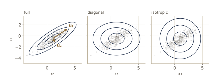
The two eigenvalues multiply to the determinant, and the Mahalanobis distance computed in the rotated coordinates matches the direct formula. The first panel of the figure below draws this Gaussian: the long axis of the ellipses points along the eigenvector with eigenvalue 2.8, the short axis along the one with eigenvalue 0.2.
Moments
Substituting \(\mathbf{z} = \mathbf{x} - \boldsymbol{\mu}\) in \(\mathbb{E}[\mathbf{x}] = \int \mathcal{N}(\mathbf{x} \mid \boldsymbol{\mu}, \boldsymbol{\Sigma})\, \mathbf{x} \, d\mathbf{x}\) gives an integral of \((\mathbf{z} + \boldsymbol{\mu})\) against a density that is even in \(\mathbf{z}\). The \(\mathbf{z}\) term vanishes by symmetry, so \(\mathbb{E}[\mathbf{x}] = \boldsymbol{\mu}\). For the second moment, the cross terms vanish the same way and the \(\mathbf{z}\mathbf{z}^{\mathrm{T}}\) term is evaluated in the eigen-coordinates, where the components are independent with variances \(\lambda_i\):
\[\mathbb{E}[\mathbf{x}\mathbf{x}^{\mathrm{T}}] = \boldsymbol{\mu}\boldsymbol{\mu}^{\mathrm{T}} + \boldsymbol{\Sigma}, \qquad \operatorname{cov}[\mathbf{x}] = \mathbb{E}\bigl[(\mathbf{x} - \mathbb{E}[\mathbf{x}])(\mathbf{x} - \mathbb{E}[\mathbf{x}])^{\mathrm{T}}\bigr] = \boldsymbol{\Sigma}.\]So the parameters are exactly the mean and the covariance. A Monte Carlo check with our sampler:
S = gaussian_sample(mu2, Sigma2, 200_000, rng)
print("sample mean:", S.mean(axis=0))
print("sample E[x x^T]:\n", S.T @ S / len(S))
print("mu mu^T + Sigma:\n", np.outer(mu2, mu2) + Sigma2)
Yc = (S - mu2) @ U                                   # eigen-coordinates of every sample
print("covariance in eigen-coordinates:\n", np.cov(Yc.T))
sample mean: [ 0.9961 -0.5039]
sample E[x x^T]:
 [[3.0017 0.7035]
 [0.7035 1.2573]]
mu mu^T + Sigma:
 [[3.   0.7 ]
 [0.7  1.25]]
covariance in eigen-coordinates:
 [[ 0.2002 -0.0007]
 [-0.0007  2.8126]]
In the eigen-coordinates the sample covariance is diagonal, up to Monte Carlo error, with the eigenvalues on the diagonal: the rotated components are uncorrelated.
Limitations
A symmetric \(D \times D\) covariance has \(D(D + 1)/2\) free entries; with the mean, a Gaussian has \(D(D + 3)/2\) parameters, which grows quadratically with \(D\), and working with \(\boldsymbol{\Sigma}\) costs \(O(D^3)\) for a factorization. Two restricted forms are common. A diagonal covariance \(\boldsymbol{\Sigma} = \operatorname{diag}(\sigma_i^2)\) has \(2D\) parameters and axis-aligned ellipses; an isotropic covariance \(\boldsymbol{\Sigma} = \sigma^2\mathbf{I}\) has \(D + 1\) parameters and spherical contours. Both are cheap, and both throw away the correlations between variables. The figure above shows all three.
The second limitation is structural: a Gaussian is unimodal, with a single peak, so it cannot represent data that fall into several clumps. The Gaussian is thus too flexible in one sense and too rigid in another. Latent variables address both: discrete latent variables give the mixtures later in this section and in module 15, and continuous latent variables give models whose number of parameters is controlled separately from \(D\) (module 16).
The cell below counts parameters at the size of an MNIST image (\(D = 784\)) and then compares the three forms on held-out data in \(D = 10\), fitting each by maximum likelihood (the formulas are derived below: the diagonal fit keeps the diagonal of the sample covariance, the isotropic fit its average diagonal entry).
for D in (2, 10, 784):
    print(f"D = {D:3d}: full {D * (D + 3) // 2:7d}, diagonal {2 * D:5d}, "
          f"isotropic {D + 1:4d}")

def fit_gaussian(X, kind="full"):
    """Maximum likelihood fit with a full, diagonal, or isotropic covariance."""
    mu = X.mean(axis=0)
    C = (X - mu).T @ (X - mu) / len(X)               # Sigma_ML
    if kind == "diagonal":
        C = np.diag(np.diag(C))
    elif kind == "isotropic":
        C = np.trace(C) / len(mu) * np.eye(len(mu))
    return mu, C

D = 10
A = rng.normal(size=(D, D)) / np.sqrt(D)
Sigma_true = A @ A.T + 0.1 * np.eye(D)               # a correlated covariance
X_test = gaussian_sample(np.zeros(D), Sigma_true, 5000, rng)
for Ntr in (12, 30, 1000):
    X_tr = gaussian_sample(np.zeros(D), Sigma_true, Ntr, rng)
    row = [gaussian_logpdf(X_test, *fit_gaussian(X_tr, kind)).mean()
           for kind in ("full", "diagonal", "isotropic")]
    print(f"N = {Ntr:4d}: test log-lik per point  full {row[0]:8.2f}   "
          f"diagonal {row[1]:7.2f}   isotropic {row[2]:7.2f}")
print(f"true Sigma: {gaussian_logpdf(X_test, np.zeros(D), Sigma_true).mean():.2f}")
D =   2: full       5, diagonal     4, isotropic    3
D =  10: full      65, diagonal    20, isotropic   11
D = 784: full  308504, diagonal  1568, isotropic  785
N =   12: test log-lik per point  full   -49.83   diagonal  -15.53   isotropic  -15.45
N =   30: test log-lik per point  full   -14.90   diagonal  -14.96   isotropic  -15.03
N = 1000: test log-lik per point  full   -12.52   diagonal  -14.72   isotropic  -14.92
true Sigma: -12.48
A full covariance for \(28 \times 28\) images needs over 300,000 parameters. On the ten-dimensional data the trade-off is visible directly. With only 12 training points the full covariance, estimated from barely more points than dimensions, is badly overfit and scores far worse on test data than the restricted forms. By 30 points the three are about even, and with 1000 points the full covariance is the clear winner and comes close to the true one. Choosing a covariance structure is a model-complexity decision like any other.
Conditional distributions
Partition \(\mathbf{x}\) into two groups, \(\mathbf{x}_a\) (the first \(M\) components) and \(\mathbf{x}_b\) (the rest), and partition the mean and covariance to match:
\[\mathbf{x} = \begin{pmatrix} \mathbf{x}_a \\ \mathbf{x}_b \end{pmatrix}, \qquad \boldsymbol{\mu} = \begin{pmatrix} \boldsymbol{\mu}_a \\ \boldsymbol{\mu}_b \end{pmatrix}, \qquad \boldsymbol{\Sigma} = \begin{pmatrix} \boldsymbol{\Sigma}_{aa} & \boldsymbol{\Sigma}_{ab} \\ \boldsymbol{\Sigma}_{ba} & \boldsymbol{\Sigma}_{bb} \end{pmatrix}.\]It helps to work also with the precision matrix \(\boldsymbol{\Lambda} = \boldsymbol{\Sigma}^{-1}\), partitioned the same way. Its blocks are not the inverses of the covariance blocks: \(\boldsymbol{\Lambda}_{aa} \ne \boldsymbol{\Sigma}_{aa}^{-1}\) in general.
If \(\mathbf{x}_a\) and \(\mathbf{x}_b\) are jointly Gaussian, the conditional \(p(\mathbf{x}_a \mid \mathbf{x}_b)\) is Gaussian too. The argument is short. As a function of \(\mathbf{x}_a\) with \(\mathbf{x}_b\) fixed, the conditional is proportional to the joint, and the joint’s exponent \(-\frac{1}{2}(\mathbf{x} - \boldsymbol{\mu})^{\mathrm{T}}\boldsymbol{\Lambda}(\mathbf{x} - \boldsymbol{\mu})\), written out in blocks, is a quadratic function of \(\mathbf{x}_a\). Any Gaussian’s exponent expands as \(-\frac{1}{2}\mathbf{x}^{\mathrm{T}}\boldsymbol{\Sigma}^{-1}\mathbf{x} + \mathbf{x}^{\mathrm{T}}\boldsymbol{\Sigma}^{-1}\boldsymbol{\mu} + \text{const}\), so we can read off the inverse covariance from the second-order term and the mean from the first-order term. This is called completing the square. The second-order term in \(\mathbf{x}_a\) is \(-\frac{1}{2}\mathbf{x}_a^{\mathrm{T}}\boldsymbol{\Lambda}_{aa}\mathbf{x}_a\) and the first-order term is \(\mathbf{x}_a^{\mathrm{T}}\{\boldsymbol{\Lambda}_{aa}\boldsymbol{\mu}_a - \boldsymbol{\Lambda}_{ab}(\mathbf{x}_b - \boldsymbol{\mu}_b)\}\), which gives the precision form of the result below. The inverse of a partitioned matrix (via the Schur complement \(\boldsymbol{\Sigma}_{aa} - \boldsymbol{\Sigma}_{ab}\boldsymbol{\Sigma}_{bb}^{-1}\boldsymbol{\Sigma}_{ba}\)) converts it to the covariance form. Intro to ML, module 02 does every step.
Result. For a jointly Gaussian \(\mathbf{x} = (\mathbf{x}_a, \mathbf{x}_b)\), the conditional is \(p(\mathbf{x}_a \mid \mathbf{x}_b) = \mathcal{N}(\mathbf{x}_a \mid \boldsymbol{\mu}_{a \mid b}, \boldsymbol{\Sigma}_{a \mid b})\) with
\[\begin{aligned} \boldsymbol{\mu}_{a \mid b} &= \boldsymbol{\mu}_a + \boldsymbol{\Sigma}_{ab}\boldsymbol{\Sigma}_{bb}^{-1}(\mathbf{x}_b - \boldsymbol{\mu}_b) = \boldsymbol{\mu}_a - \boldsymbol{\Lambda}_{aa}^{-1}\boldsymbol{\Lambda}_{ab}(\mathbf{x}_b - \boldsymbol{\mu}_b), \\ \boldsymbol{\Sigma}_{a \mid b} &= \boldsymbol{\Sigma}_{aa} - \boldsymbol{\Sigma}_{ab}\boldsymbol{\Sigma}_{bb}^{-1}\boldsymbol{\Sigma}_{ba} = \boldsymbol{\Lambda}_{aa}^{-1}. \end{aligned}\]
The conditional mean is a linear function of the observed \(\mathbf{x}_b\), and the conditional covariance does not depend on \(\mathbf{x}_b\) at all and is never larger than \(\boldsymbol{\Sigma}_{aa}\): observing correlated variables can only reduce uncertainty. A conditional whose mean is linear in the conditioning variable and whose covariance is constant is a linear-Gaussian model, the building block of the next subsection.
We check the result exactly on a three-dimensional Gaussian, conditioning \(x_1\) on \((x_2, x_3)\). The covariance and precision forms must agree, and, more to the point, the conditional density must equal the joint divided by the marginal of \(\mathbf{x}_b\) at every value of \(x_1\) (the marginal formula is the subject of the subsection after next; here we use it as given).
mu3 = np.array([0.5, -1.0, 2.0])
Sigma3 = np.array([[1.5, 0.6, -0.4],
                   [0.6, 1.0, 0.3],
                   [-0.4, 0.3, 0.8]])
a, b = [0], [1, 2]                                  # x_a = x_1, x_b = (x_2, x_3)

def gaussian_conditional(mu, Sigma, a, b, x_b):
    """Mean and covariance of p(x_a | x_b) from the covariance blocks."""
    S_ab, S_bb = Sigma[np.ix_(a, b)], Sigma[np.ix_(b, b)]
    gain = np.linalg.solve(S_bb, S_ab.T).T          # Sigma_ab Sigma_bb^{-1}
    mean = mu[a] + gain @ (x_b - mu[b])
    cov = Sigma[np.ix_(a, a)] - gain @ S_ab.T
    return mean, cov

x_b = np.array([-0.2, 1.5])
m_cov, C_cov = gaussian_conditional(mu3, Sigma3, a, b, x_b)
Lam = np.linalg.inv(Sigma3)                         # precision, to check the other form
L_aa, L_ab = Lam[np.ix_(a, a)], Lam[np.ix_(a, b)]
m_prec = mu3[a] - np.linalg.solve(L_aa, L_ab @ (x_b - mu3[b]))
print(f"covariance form: mean {m_cov[0]:.4f}, variance {C_cov[0, 0]:.4f}")
print(f"precision form : mean {m_prec[0]:.4f}, variance {1 / L_aa[0, 0]:.4f}")

xa_grid = np.linspace(-3, 4, 7)[:, None]
joint = gaussian_logpdf(np.hstack([xa_grid, np.tile(x_b, (7, 1))]), mu3, Sigma3)
marg_b = gaussian_logpdf(x_b, mu3[b], Sigma3[np.ix_(b, b)])
cond = gaussian_logpdf(xa_grid, m_cov, C_cov)
print("ln p(x_a, x_b) - ln p(x_b) equals ln N(x_a | mu_a|b, Sigma_a|b):",
      np.allclose(joint - marg_b, cond))
covariance form: mean 1.5845, variance 0.6662
precision form : mean 1.5845, variance 0.6662
ln p(x_a, x_b) - ln p(x_b) equals ln N(x_a | mu_a|b, Sigma_a|b): True
There is also a neat sampling check that connects to regression. Since \(\mathbb{E}[x_1 \mid x_2, x_3]\) is linear in \((x_2, x_3)\) with slopes \(\boldsymbol{\Sigma}_{ab}\boldsymbol{\Sigma}_{bb}^{-1}\), a least-squares fit of \(x_1\) on \((1, x_2, x_3)\) over many joint samples should recover those slopes, and the variance of its residuals should be \(\boldsymbol{\Sigma}_{a \mid b}\).
Z3 = gaussian_sample(mu3, Sigma3, 100_000, rng)
Phi = np.column_stack([np.ones(len(Z3)), Z3[:, b]])       # regress x_1 on (1, x_2, x_3)
w, *_ = np.linalg.lstsq(Phi, Z3[:, 0], rcond=None)
resid = Z3[:, 0] - Phi @ w
gain = np.linalg.solve(Sigma3[np.ix_(b, b)], Sigma3[np.ix_(a, b)].T).ravel()
print("least-squares slopes:", w[1:], "  Sigma_ab Sigma_bb^-1:", gain)
print(f"residual variance {resid.var():.4f}   Sigma_a|b {C_cov[0, 0]:.4f}")
least-squares slopes: [ 0.8443 -0.8165]   Sigma_ab Sigma_bb^-1: [ 0.8451 -0.8169]
residual variance 0.6634   Sigma_a|b 0.6662
For jointly Gaussian data, linear regression with Gaussian noise is not an approximation: it is the exact conditional distribution. Module 04 starts from this kind of model.
Marginal distributions
The marginal \(p(\mathbf{x}_a) = \int p(\mathbf{x}_a, \mathbf{x}_b)\, d\mathbf{x}_b\) is also Gaussian, and it has the simplest possible answer:
\[p(\mathbf{x}_a) = \mathcal{N}(\mathbf{x}_a \mid \boldsymbol{\mu}_a, \boldsymbol{\Sigma}_{aa}).\]To integrate out a group of Gaussian variables, just delete their rows and columns. The derivation completes the square in \(\mathbf{x}_b\) so that the integral over \(\mathbf{x}_b\) becomes the normalizer of a Gaussian, which does not depend on \(\mathbf{x}_a\); what remains is quadratic in \(\mathbf{x}_a\) with precision \(\boldsymbol{\Lambda}_{aa} - \boldsymbol{\Lambda}_{ab}\boldsymbol{\Lambda}_{bb}^{-1}\boldsymbol{\Lambda}_{ba}\), and the partitioned-inverse formula shows that this is \(\boldsymbol{\Sigma}_{aa}^{-1}\). Notice the contrast: the conditional is simplest in terms of the precision, the marginal in terms of the covariance.
We verify it by doing the integral numerically. Integrating the three-dimensional density over \(x_1\) at a fixed \((x_2, x_3)\) should give the two-dimensional Gaussian with the \((x_2, x_3)\) block of the mean and covariance.
u = np.linspace(-9, 10, 4001)                         # quadrature grid for x_1
x23 = np.array([0.3, 2.4])
pts = np.column_stack([u, np.tile(x23, (len(u), 1))])
integral = np.trapezoid(np.exp(gaussian_logpdf(pts, mu3, Sigma3)), u)
marg = np.exp(gaussian_logpdf(x23, mu3[b], Sigma3[np.ix_(b, b)]))[0]
print(f"integral over x_1 of p(x_1, x_2, x_3) = {integral:.6f};  "
      f"N(x_b | mu_b, Sigma_bb) = {marg:.6f}")
integral over x_1 of p(x_1, x_2, x_3) = 0.081130; N(x_b | mu_b, Sigma_bb) = 0.081130
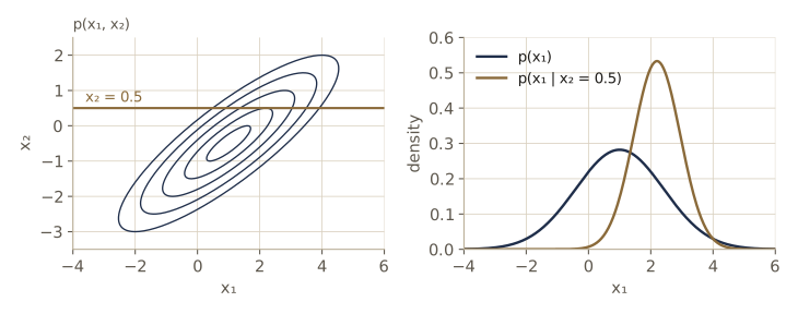
The figure shows both operations on the two-dimensional Gaussian from the geometry section: slicing the joint along a line \(x_2 = 0.5\) and renormalizing gives the conditional, while integrating over \(x_2\) gives the wider marginal.
Bayes’ theorem for linear-Gaussian models
Now suppose we are given the two pieces separately: a Gaussian marginal for \(\mathbf{x}\) (dimension \(M\)) and a Gaussian conditional for \(\mathbf{y}\) (dimension \(D\)) whose mean is a linear function of \(\mathbf{x}\),
\[p(\mathbf{x}) = \mathcal{N}(\mathbf{x} \mid \boldsymbol{\mu}, \boldsymbol{\Lambda}^{-1}), \qquad p(\mathbf{y} \mid \mathbf{x}) = \mathcal{N}(\mathbf{y} \mid \mathbf{A}\mathbf{x} + \mathbf{b}, \mathbf{L}^{-1}),\]with \(\mathbf{A}\) of size \(D \times M\) and precision matrices \(\boldsymbol{\Lambda}\) and \(\mathbf{L}\). Read \(\mathbf{x}\) as a hidden quantity with a prior, and \(\mathbf{y}\) as a noisy linear measurement of it. We want the evidence \(p(\mathbf{y})\) and the posterior \(p(\mathbf{x} \mid \mathbf{y})\).
The route is to recognize that \(\mathbf{z} = (\mathbf{x}, \mathbf{y})\) is jointly Gaussian: \(\ln p(\mathbf{x}) + \ln p(\mathbf{y} \mid \mathbf{x})\) is quadratic in \(\mathbf{z}\). Completing the square gives its mean and covariance,
\[\mathbb{E}[\mathbf{z}] = \begin{pmatrix} \boldsymbol{\mu} \\ \mathbf{A}\boldsymbol{\mu} + \mathbf{b} \end{pmatrix}, \qquad \operatorname{cov}[\mathbf{z}] = \begin{pmatrix} \boldsymbol{\Lambda}^{-1} & \boldsymbol{\Lambda}^{-1}\mathbf{A}^{\mathrm{T}} \\ \mathbf{A}\boldsymbol{\Lambda}^{-1} & \mathbf{L}^{-1} + \mathbf{A}\boldsymbol{\Lambda}^{-1}\mathbf{A}^{\mathrm{T}} \end{pmatrix},\]and then the marginal and conditional results of the last two subsections finish the job.
Result. For the linear-Gaussian model above,
\[\begin{aligned} p(\mathbf{y}) &= \mathcal{N}(\mathbf{y} \mid \mathbf{A}\boldsymbol{\mu} + \mathbf{b}, \ \mathbf{L}^{-1} + \mathbf{A}\boldsymbol{\Lambda}^{-1}\mathbf{A}^{\mathrm{T}}), \\ p(\mathbf{x} \mid \mathbf{y}) &= \mathcal{N}\bigl(\mathbf{x} \mid \boldsymbol{\Sigma}\{\mathbf{A}^{\mathrm{T}}\mathbf{L}(\mathbf{y} - \mathbf{b}) + \boldsymbol{\Lambda}\boldsymbol{\mu}\}, \ \boldsymbol{\Sigma}\bigr), \qquad \boldsymbol{\Sigma} = (\boldsymbol{\Lambda} + \mathbf{A}^{\mathrm{T}}\mathbf{L}\mathbf{A})^{-1}. \end{aligned}\]
Read the posterior this way: its precision is the prior precision plus the precision the measurement contributes, and its mean is a precision-weighted blend of the prior mean and what the data say. The evidence covariance is the measurement noise plus the prior spread pushed through \(\mathbf{A}\). This one result appears all over the book: Bayesian linear regression, probabilistic PCA and factor analysis (module 16), the forward and reverse steps of diffusion models (module 20), and the Kalman filter (Intro to ML, module 13).
Let’s check it with a two-dimensional \(\mathbf{x}\) observed through three noisy linear sensors. We compute the posterior once with the formula, and once by building the joint covariance of \(\mathbf{z}\) explicitly and calling gaussian_conditional from before.
mu_x = np.array([0.0, 1.0])
Lam_x = np.linalg.inv(np.array([[1.0, 0.5], [0.5, 2.0]]))   # prior precision Lambda
A_lg = np.array([[1.0, 0.0], [1.0, -1.0], [0.5, 2.0]])      # D = 3 by M = 2
b_lg = np.array([0.2, 0.0, -1.0])
L_lg = np.diag([4.0, 1.0, 10.0])                             # noise precision L

def linear_gaussian(mu, Lam, A, b, L, y):
    """p(y) and p(x | y) for p(x) = N(mu, Lam^-1) and p(y | x) = N(Ax + b, L^-1)."""
    py_mean = A @ mu + b
    py_cov = np.linalg.inv(L) + A @ np.linalg.solve(Lam, A.T)
    post_cov = np.linalg.inv(Lam + A.T @ L @ A)          # Sigma = (Lambda + A^T L A)^-1
    post_mean = post_cov @ (A.T @ L @ (y - b) + Lam @ mu)
    return py_mean, py_cov, post_mean, post_cov

y_obs = np.array([0.5, -1.0, 1.2])
py_m, py_C, px_m, px_C = linear_gaussian(mu_x, Lam_x, A_lg, b_lg, L_lg, y_obs)

Sx = np.linalg.inv(Lam_x)                                    # joint over z = (x, y)
mu_z = np.concatenate([mu_x, A_lg @ mu_x + b_lg])
Sigma_z = np.block([[Sx, Sx @ A_lg.T],
                    [A_lg @ Sx, np.linalg.inv(L_lg) + A_lg @ Sx @ A_lg.T]])
m_j, C_j = gaussian_conditional(mu_z, Sigma_z, [0, 1], [2, 3, 4], y_obs)
print("posterior mean:", px_m, "  via the joint:", m_j)
print("posterior covariance:\n", px_C, "\nvia the joint:\n", C_j)
print("p(y) covariance matches the joint:", np.allclose(py_C, Sigma_z[2:, 2:]))
print("prior variances:", np.diag(Sx), "  posterior variances:", np.diag(px_C))
posterior mean: [0.1997 1.0543]   via the joint: [0.1997 1.0543]
posterior covariance:
 [[ 0.1467 -0.0308]
 [-0.0308  0.0305]]
via the joint:
 [[ 0.1467 -0.0308]
 [-0.0308  0.0305]]
p(y) covariance matches the joint: True
prior variances: [1. 2.]   posterior variances: [0.1467 0.0305]
Both routes give the same posterior to every printed digit, and three measurements shrink the prior variances by a large factor.
Maximum likelihood
Given \(N\) i.i.d. observations stacked as the rows of \(\mathbf{X}\), the Gaussian log-likelihood is
\[\ln p(\mathbf{X} \mid \boldsymbol{\mu}, \boldsymbol{\Sigma}) = -\frac{ND}{2}\ln(2\pi) - \frac{N}{2}\ln\lvert\boldsymbol{\Sigma}\rvert - \frac{1}{2}\sum_{n=1}^{N}(\mathbf{x}_n - \boldsymbol{\mu})^{\mathrm{T}}\boldsymbol{\Sigma}^{-1}(\mathbf{x}_n - \boldsymbol{\mu}).\]Expanding the quadratic form shows that the data enter only through \(\sum_n \mathbf{x}_n\) and \(\sum_n \mathbf{x}_n\mathbf{x}_n^{\mathrm{T}}\), the sufficient statistics of the Gaussian. The gradient with respect to the mean is \(\sum_n \boldsymbol{\Sigma}^{-1}(\mathbf{x}_n - \boldsymbol{\mu})\), and setting it to zero gives the sample mean. Maximizing over \(\boldsymbol{\Sigma}\) takes a few matrix-derivative identities (ignore the symmetry constraint, and the answer turns out symmetric anyway; see Intro to ML, module 02):
\[\boldsymbol{\mu}_{\mathrm{ML}} = \frac{1}{N}\sum_{n=1}^{N}\mathbf{x}_n, \qquad \boldsymbol{\Sigma}_{\mathrm{ML}} = \frac{1}{N}\sum_{n=1}^{N}(\mathbf{x}_n - \boldsymbol{\mu}_{\mathrm{ML}})(\mathbf{x}_n - \boldsymbol{\mu}_{\mathrm{ML}})^{\mathrm{T}}.\]The mean estimate is unbiased, \(\mathbb{E}[\boldsymbol{\mu}_{\mathrm{ML}}] = \boldsymbol{\mu}\), but the covariance estimate is not: \(\mathbb{E}[\boldsymbol{\Sigma}_{\mathrm{ML}}] = \frac{N - 1}{N}\boldsymbol{\Sigma}\). The deviations are measured from the sample mean, which was fitted to the same data and so sits closer to them than the true mean does. Dividing by \(N - 1\) instead of \(N\) removes the bias. The bias matters only when \(N\) is small, so we check it with many tiny data sets of five points each.
def gaussian_ml(X):
    mu = X.mean(axis=0)
    return mu, (X - mu).T @ (X - mu) / len(X)

R, Nsmall = 40_000, 5
Xsets = gaussian_sample(mu2, Sigma2, R * Nsmall, rng).reshape(R, Nsmall, 2)
dev = Xsets - Xsets.mean(axis=1, keepdims=True)
Sigma_ml_avg = np.einsum("rni,rnj->ij", dev, dev) / (R * Nsmall)   # average of Sigma_ML
print(f"average Sigma_ML over {R} data sets of N = {Nsmall}:\n", Sigma_ml_avg)
print("(N - 1)/N Sigma:\n", (Nsmall - 1) / Nsmall * Sigma2)
average Sigma_ML over 40000 data sets of N = 5:
 [[1.5995 0.9579]
 [0.9579 0.7957]]
(N - 1)/N Sigma:
 [[1.6  0.96]
 [0.96 0.8 ]]
The average of the maximum likelihood estimates matches \(\frac{4}{5}\boldsymbol{\Sigma}\), not \(\boldsymbol{\Sigma}\). The same thing happens in regression: a network trained by least squares underestimates the noise variance if we read it off the training residuals, and more so the more parameters the network has.
Sequential estimation
Maximum likelihood as written is a batch method: it looks at all the data at once. Pulling the last point out of the sample mean gives an update that processes one point at a time:
\[\boldsymbol{\mu}_{\mathrm{ML}}^{(N)} = \frac{1}{N}\sum_{n=1}^{N}\mathbf{x}_n = \boldsymbol{\mu}_{\mathrm{ML}}^{(N-1)} + \frac{1}{N}\bigl(\mathbf{x}_N - \boldsymbol{\mu}_{\mathrm{ML}}^{(N-1)}\bigr).\]The new estimate moves the old one a step of size \(1/N\) toward the new point, in the direction of the “error” \(\mathbf{x}_N - \boldsymbol{\mu}^{(N-1)}\). The steps shrink as data accumulate, and after \(N\) points the result is exactly the batch mean.
This is the simplest case of a general idea. Robbins and Monro studied updates of the form \(\theta^{(N)} = \theta^{(N-1)} + \eta_N\, g(\theta^{(N-1)}, \mathbf{x}_N)\) that look for the root of the expected value of \(g\) using one noisy sample at a time, and showed that they converge if the step sizes satisfy \(\eta_N \to 0\), \(\sum_N \eta_N = \infty\), and \(\sum_N \eta_N^2 < \infty\); the choice \(\eta_N = 1/N\) qualifies. With \(g\) the gradient of a log-likelihood term, this is stochastic gradient ascent, the engine of all network training (module 07). Deep learning often uses a constant step instead, \(\eta_N = \eta\). That gives an exponentially weighted moving average, which forgets old data at a fixed rate. It never settles exactly, but it can follow a quantity that changes over time. Adam’s running averages of gradients and batch normalization’s running statistics (both in module 07) are moving averages of this kind.
stream = rng.normal(2.0, 1.0, size=2000)
mu_run = 0.0
for n, x_n in enumerate(stream, start=1):
    mu_run += (x_n - mu_run) / n                         # step 1/N
print(f"running mean {mu_run:.6f}   batch mean {stream.mean():.6f}")

drift = np.concatenate([rng.normal(2.0, 1.0, 1000), rng.normal(-1.0, 1.0, 1000)])
mu_avg, mu_ema, eta_c = 0.0, 0.0, 0.02
for n, x_n in enumerate(drift, start=1):
    mu_avg += (x_n - mu_avg) / n                         # step 1/N
    mu_ema += eta_c * (x_n - mu_ema)                     # constant step
    if n in (500, 1000, 1100, 1500, 2000):
        print(f"n = {n:4d}: 1/N step {mu_avg:6.3f}   constant step 0.02 {mu_ema:6.3f}")
running mean 2.038880   batch mean 2.038880
n =  500: 1/N step  1.966   constant step 0.02  2.050
n = 1000: 1/N step  2.000   constant step 0.02  2.004
n = 1100: 1/N step  1.737   constant step 0.02 -0.496
n = 1500: 1/N step  1.038   constant step 0.02 -0.857
n = 2000: 1/N step  0.526   constant step 0.02 -1.029
On a stationary stream the one-point update reproduces the batch mean exactly. When the true mean jumps from 2 to \(-1\) halfway through, the \(1/N\) average is stuck with its memory of the first half and reaches only about 0.5 by the end, while the constant-step average has covered most of the distance within a hundred points and ends close to \(-1\). With step \(\eta\) it effectively averages the last \(1/\eta = 50\) or so points, so it keeps fluctuating instead of converging.
Mixtures of Gaussians
A single Gaussian puts its peak between two clumps of data, exactly where there are no points. A mixture of Gaussians combines \(K\) of them:
\[p(\mathbf{x}) = \sum_{k=1}^{K} \pi_k\, \mathcal{N}(\mathbf{x} \mid \boldsymbol{\mu}_k, \boldsymbol{\Sigma}_k).\]Each Gaussian is a component with its own mean and covariance, and the \(\pi_k\) are mixing coefficients. Integrating both sides shows \(\sum_k \pi_k = 1\), and requiring \(p(\mathbf{x}) \ge 0\) everywhere is guaranteed by \(\pi_k \ge 0\), so the mixing coefficients behave like probabilities. With enough components, a mixture can approximate essentially any continuous density.
The probabilistic reading makes this precise. Write \(p(\mathbf{x}) = \sum_k p(k)\, p(\mathbf{x} \mid k)\) with \(p(k) = \pi_k\) the probability of choosing component \(k\) and \(p(\mathbf{x} \mid k)\) that component’s Gaussian. Then Bayes’ theorem gives the posterior probability that a point came from component \(k\), its responsibility:
\[\gamma_k(\mathbf{x}) = p(k \mid \mathbf{x}) = \frac{\pi_k\, \mathcal{N}(\mathbf{x} \mid \boldsymbol{\mu}_k, \boldsymbol{\Sigma}_k)}{\sum_{j} \pi_j\, \mathcal{N}(\mathbf{x} \mid \boldsymbol{\mu}_j, \boldsymbol{\Sigma}_j)}.\]The same reading gives a sampler (pick \(k\) with probability \(\pi_k\), then draw from component \(k\)), called ancestral sampling. The log-likelihood of a data set is
\[\ln p(\mathbf{X} \mid \boldsymbol{\pi}, \boldsymbol{\mu}, \boldsymbol{\Sigma}) = \sum_{n=1}^{N} \ln \Bigl\{ \sum_{k=1}^{K} \pi_k\, \mathcal{N}(\mathbf{x}_n \mid \boldsymbol{\mu}_k, \boldsymbol{\Sigma}_k) \Bigr\}.\]The sum sits inside the logarithm, so the log no longer cancels the exponentials and there is no closed-form maximum. It can be maximized by gradient-based optimization, or by the expectation-maximization (EM) algorithm of module 15. Evaluating it safely needs log-sum-exp: each term \(\ln\pi_k + \ln\mathcal{N}(\mathbf{x}_n \mid \cdot)\) is computed in log space and combined with logsumexp.
pi_mix = np.array([0.45, 0.35, 0.20])
mu_mix = [np.array([-1.5, 0.0]), np.array([1.5, 1.0]), np.array([0.5, -2.0])]
Sigma_mix = [np.array([[0.8, 0.5], [0.5, 0.9]]),
             np.array([[0.6, -0.3], [-0.3, 0.5]]),
             np.array([[1.2, 0.0], [0.0, 0.25]])]

def gmm_log_terms(X, pis, mus, Sigmas):
    """ln pi_k + ln N(x_n | mu_k, Sigma_k), shape (N, K)."""
    return np.stack([np.log(p) + gaussian_logpdf(X, m, S)
                     for p, m, S in zip(pis, mus, Sigmas)], axis=1)

def gmm_logpdf(X, pis, mus, Sigmas):
    return logsumexp(gmm_log_terms(X, pis, mus, Sigmas), axis=1)

def gmm_responsibilities(X, pis, mus, Sigmas):
    """gamma_k(x) = pi_k N_k / sum_j pi_j N_j, computed in log space."""
    T = gmm_log_terms(X, pis, mus, Sigmas)
    return np.exp(T - logsumexp(T, axis=1, keepdims=True))

def gmm_sample(pis, mus, Sigmas, size, rng):
    """Ancestral sampling: draw the component k, then x from component k."""
    k = rng.choice(len(pis), size=size, p=pis)
    X = np.empty((size, len(mus[0])))
    for j in range(len(pis)):
        X[k == j] = gaussian_sample(mus[j], Sigmas[j], np.sum(k == j), rng)
    return X, k

g1 = np.linspace(-8, 8, 641)
G = np.array(np.meshgrid(g1, g1)).reshape(2, -1).T
area = np.exp(gmm_logpdf(G, pi_mix, mu_mix, Sigma_mix)).sum() * (g1[1] - g1[0]) ** 2
print(f"mixture density sums to {area:.4f} over a grid")
probe = np.array([[-1.5, 0.0], [0.0, 1.0], [30.0, -25.0]])
print("responsibilities:\n", gmm_responsibilities(probe, pi_mix, mu_mix, Sigma_mix))
with np.errstate(divide="ignore"):
    naive = np.log(np.exp(gmm_log_terms(probe, pi_mix, mu_mix, Sigma_mix)).sum(axis=1))
print("naive log density:", naive)
print("log-sum-exp      :", gmm_logpdf(probe, pi_mix, mu_mix, Sigma_mix))
Xm, km = gmm_sample(pi_mix, mu_mix, Sigma_mix, 600, rng)
mu1, S1 = gaussian_ml(Xm)
print(f"mean log-lik: single Gaussian (ML) {gaussian_logpdf(Xm, mu1, S1).mean():.4f}, "
      f"the mixture {gmm_logpdf(Xm, pi_mix, mu_mix, Sigma_mix).mean():.4f}")
mixture density sums to 1.0000 over a grid
responsibilities:
 [[1.     0.     0.    ]
 [0.7535 0.2465 0.    ]
 [0.     1.     0.    ]]
naive log density: [-2.2588 -3.3855    -inf]
log-sum-exp      : [  -2.2588   -3.3855 -876.2145]
mean log-lik: single Gaussian (ML) -3.6167, the mixture -3.2329
A point at the center of the first component belongs to it with near certainty; a point between the first two components gets split responsibility. For a point far from all components, every term underflows to zero in the naive computation and its log is \(-\infty\), while log-sum-exp returns the correct large negative number. That matters in training: a single \(-\infty\) turns the loss and every gradient into nan. On the 600 samples, the best single Gaussian has a clearly lower log-likelihood than the mixture that generated them.
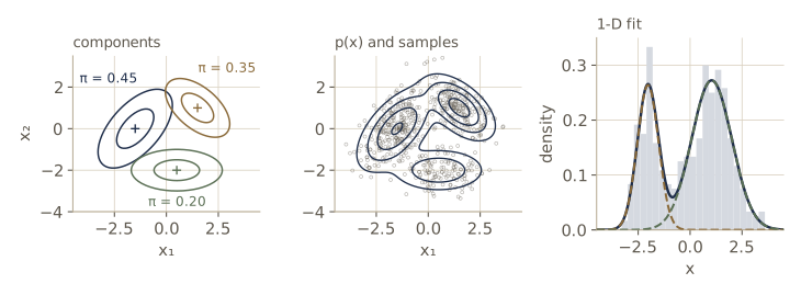
Fitting a mixture by gradient ascent shows how a network would do it. The parameters have constraints (\(\pi_k\) on the simplex, \(\sigma_k > 0\)), so we optimize unconstrained quantities instead: logits \(\eta_k\) with \(\boldsymbol{\pi} = \operatorname{softmax}(\boldsymbol{\eta})\), and \(s_k = \ln\sigma_k\). This is exactly how a mixture density network (module 06) parametrizes its outputs, with a network computing \(\eta_k\), \(\mu_k\), and \(s_k\) from each input. The gradients of the log-likelihood take a tidy form in terms of the responsibilities \(\gamma_{nk}\) and the standardized residuals \(z_{nk} = (x_n - \mu_k)/\sigma_k\):
\[\frac{\partial \ln p}{\partial \eta_k} = \sum_n (\gamma_{nk} - \pi_k), \qquad \frac{\partial \ln p}{\partial \mu_k} = \sum_n \gamma_{nk} \frac{z_{nk}}{\sigma_k}, \qquad \frac{\partial \ln p}{\partial s_k} = \sum_n \gamma_{nk}(z_{nk}^2 - 1).\]Each is the gradient of a single Gaussian (or of a softmax) weighted by how responsible component \(k\) is for point \(n\). We check them with finite differences and then run plain gradient ascent on the mean log-likelihood for 400 one-dimensional points from a two-component mixture.
def mix1d_loglik_grad(x, eta, mu, s):
    """Mean log-likelihood and its gradients w.r.t. eta, mu, and s = ln sigma."""
    log_pi = eta - logsumexp(eta)
    z = (x[:, None] - mu) / np.exp(s)                 # standardized residuals z_nk
    T = log_pi - 0.5 * np.log(2 * np.pi) - s - 0.5 * z ** 2
    ll = logsumexp(T, axis=1)
    gam = np.exp(T - ll[:, None])                     # responsibilities gamma_nk
    g_eta = (gam - np.exp(log_pi)).mean(axis=0)
    g_mu = (gam * z / np.exp(s)).mean(axis=0)
    g_s = (gam * (z ** 2 - 1)).mean(axis=0)
    return ll.mean(), [g_eta, g_mu, g_s]

rng_f = np.random.default_rng(11)
comp = rng_f.random(400) < 0.3
x1 = np.where(comp, rng_f.normal(-2.0, 0.5, 400), rng_f.normal(1.0, 1.0, 400))
print(f"fraction of points drawn from the first component: {comp.mean():.3f}")
params = [np.zeros(2), np.array([-0.5, 0.5]), np.zeros(2)]      # eta, mu, s

_, grads = mix1d_loglik_grad(x1, *params)               # finite-difference check
h, err = 1e-6, 0.0
for i in range(3):
    for j in range(2):
        up = [q.copy() for q in params]; up[i][j] += h
        dn = [q.copy() for q in params]; dn[i][j] -= h
        fd = (mix1d_loglik_grad(x1, *up)[0] - mix1d_loglik_grad(x1, *dn)[0]) / (2 * h)
        err = max(err, abs(fd - grads[i][j]))
print(f"largest gradient error: {err:.1e}")

for step in range(3001):
    ll, grads = mix1d_loglik_grad(x1, *params)
    for q, g in zip(params, grads):
        q += 0.1 * g                                             # gradient ascent
    if step in (0, 100, 500, 3000):
        eta, mu, s = params
        pi = np.exp(eta - logsumexp(eta))
        print(f"step {step:4d}: mean log-lik {ll:.4f}  pi {pi}"
              f"  mu {mu}  sigma {np.exp(s)}")
fraction of points drawn from the first component: 0.333
largest gradient error: 3.1e-10
step    0: mean log-lik -2.1526  pi [0.4995 0.5005]  mu [-0.5272  0.5264]  sigma [1.0669 1.0388]
step  100: mean log-lik -1.8702  pi [0.5346 0.4654]  mu [-0.9696  1.1967]  sigma [1.4086 0.9112]
step  500: mean log-lik -1.7540  pi [0.3389 0.6611]  mu [-2.0272  1.0395]  sigma [0.5129 0.9677]
step 3000: mean log-lik -1.7540  pi [0.3379 0.6621]  mu [-2.029   1.0372]  sigma [0.5111 0.9695]
The analytic gradients agree with finite differences to about ten digits, and after a few hundred steps the fit is close to the generating mixture (weights 0.3 and 0.7, means \(-2\) and 1, standard deviations 0.5 and 1); the fitted weight of the first component is near the fraction of points that actually came from it. The right panel of the figure above shows the result. Two warnings carry over to mixture density networks: the log-likelihood has several local maxima (swapping the labels of two components gives an equally good solution), and it is unbounded above, since a component that shrinks onto a single data point drives \(\sigma_k \to 0\) and the likelihood to infinity. Module 15 returns to both.
Periodic variables
Some quantities live on a circle: a wind direction, the hour of the day, the day of the year, the angle of a joint. Represent one by an angle \(\theta \in [0, 2\pi)\). Treating \(\theta\) as an ordinary real number makes every answer depend on where we put the zero. Consider 30 synthetic wind directions clustered around north-northwest, some just east of north (a few degrees) and some just west (in the 340s and 350s). Their ordinary average, in degrees, lands far from where the wind actually blows.
The fix is to treat each angle as a point on the unit circle, \(\mathbf{x}_n = (\cos\theta_n, \sin\theta_n)\), average those vectors, and take the angle of the average. Writing the average as \(\bar{\mathbf{x}} = (\bar{r}\cos\bar{\theta}, \bar{r}\sin\bar{\theta})\),
\[\bar{\theta} = \operatorname{atan2}\Bigl(\sum_n \sin\theta_n, \ \sum_n \cos\theta_n\Bigr), \qquad \bar{r} = \frac{1}{N}\Bigl\lVert \sum_n \mathbf{x}_n \Bigr\rVert,\]where \(\operatorname{atan2}\) is the arctangent that returns the angle in the correct quadrant. The circular mean \(\bar{\theta}\) does not depend on the origin, and the mean resultant length \(\bar{r} \in [0, 1]\) measures how concentrated the angles are (1 when they all agree).
rng_w = np.random.default_rng(29)
wind = np.rad2deg(rng_w.vonmises(np.deg2rad(-15.0), 5.0, size=30)) % 360   # in [0, 360)

def circular_mean_deg(deg):
    th = np.deg2rad(deg)
    return np.rad2deg(np.arctan2(np.sin(th).sum(), np.cos(th).sum())) % 360

print(f"directions range from {wind.min():.1f} to {wind.max():.1f} deg")
for origin in (0.0, 90.0, 180.0):
    shifted = (wind - origin) % 360                 # the same directions, zero moved
    naive = (shifted.mean() + origin) % 360
    circ = (circular_mean_deg(shifted) + origin) % 360
    print(f"zero at {origin:5.1f} deg: naive mean {naive:6.1f} deg, "
          f"circular mean {circ:6.1f} deg")
directions range from 2.3 to 358.3 deg
zero at   0.0 deg: naive mean  228.6 deg, circular mean  348.4 deg
zero at  90.0 deg: naive mean  348.6 deg, circular mean  348.4 deg
zero at 180.0 deg: naive mean  348.6 deg, circular mean  348.4 deg
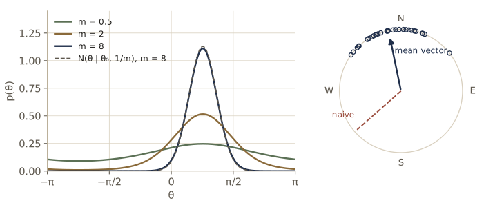
With the zero at north, the naive average points roughly southwest, while the circular mean is the same in every coordinate system. Moving the zero away from the data happens to rescue the naive average here, but only because the cut then falls where there are no observations.
In practice. When an input feature is periodic (time of day, day of week, a compass heading), feed a network the pair \((\cos\theta, \sin\theta)\) rather than \(\theta\) itself. Then 23:59 and 00:01 are neighbors, as they should be. The sinusoidal positional encodings of transformers (module 12) use sines and cosines of positions for related reasons.
The von Mises distribution
We want a Gaussian-like density on the circle: \(p(\theta) \ge 0\), \(\int_0^{2\pi} p(\theta)\, d\theta = 1\), and \(p(\theta + 2\pi) = p(\theta)\). One construction starts from an isotropic two-dimensional Gaussian with variance \(\sigma^2\) whose mean, in polar coordinates, is \((r_0\cos\theta_0, r_0\sin\theta_0)\), and restricts it to the unit circle \(\mathbf{x} = (\cos\theta, \sin\theta)\). In the exponent, \(\lVert\mathbf{x}\rVert^2 = 1\) and \(\cos\theta\cos\theta_0 + \sin\theta\sin\theta_0 = \cos(\theta - \theta_0)\), so everything except \((r_0/\sigma^2)\cos(\theta - \theta_0)\) is constant. Normalizing gives the von Mises distribution
\[p(\theta \mid \theta_0, m) = \frac{1}{2\pi I_0(m)} \exp\{m\cos(\theta - \theta_0)\}, \qquad I_0(m) = \frac{1}{2\pi}\int_0^{2\pi} \exp\{m\cos\theta\}\, d\theta.\]Here \(\theta_0\) is the mean direction and \(m = r_0/\sigma^2 \ge 0\) is the concentration, which plays the role of a precision. The normalizer \(I_0\) is the modified Bessel function of the first kind of order zero. At \(m = 0\) the distribution is uniform on the circle; for large \(m\), expanding \(\cos\alpha \approx 1 - \alpha^2/2\) shows it approaches a Gaussian in \(\theta\) with mean \(\theta_0\) and variance \(1/m\) (exercise 7).
The log-likelihood of angles \(\theta_1, \dots, \theta_N\) is
\[\ln p(\mathcal{D} \mid \theta_0, m) = -N\ln(2\pi) - N\ln I_0(m) + m\sum_{n=1}^{N}\cos(\theta_n - \theta_0).\]Setting the derivative with respect to \(\theta_0\) to zero gives \(\sum_n \sin(\theta_n - \theta_0) = 0\), whose solution (expand the sine of a difference) is \(\theta_0^{\mathrm{ML}} = \operatorname{atan2}(\sum_n \sin\theta_n, \sum_n\cos\theta_n)\): the circular mean. For the concentration, \(I_0'(m) = I_1(m)\) gives the condition
\[A(m_{\mathrm{ML}}) = \frac{1}{N}\sum_{n=1}^{N}\cos(\theta_n - \theta_0^{\mathrm{ML}}) = \bar{r}, \qquad A(m) = \frac{I_1(m)}{I_0(m)},\]so the fitted concentration is the one whose Bessel ratio equals the mean resultant length. \(A\) increases from 0 to 1, so we invert it numerically with a few Newton steps on \(\ln m\), using \(A'(m) = 1 - A(m)/m - A(m)^2\). For numerical safety we use SciPy’s exponentially scaled Bessel functions i0e(m) \(= e^{-m}I_0(m)\) and i1e.
def von_mises_logpdf(theta, theta0, m):
    """ln p(theta | theta0, m); i0e(m) = exp(-m) I0(m) keeps ln I0 finite."""
    return m * np.cos(theta - theta0) - np.log(2 * np.pi) - (np.log(i0e(m)) + m)

def A_ratio(m):
    return i1e(m) / i0e(m)                               # A(m) = I1(m) / I0(m)

def fit_von_mises(theta):
    """theta0_ML = atan2(sum sin, sum cos); m_ML solves A(m) = rbar (Newton on ln m)."""
    S, C = np.sin(theta).sum(), np.cos(theta).sum()
    theta0, rbar = np.arctan2(S, C), np.hypot(S, C) / len(theta)
    log_m = 0.0
    for _ in range(50):
        m = np.exp(log_m)
        A = A_ratio(m)
        log_m -= (A - rbar) / ((1 - A / m - A ** 2) * m)    # dA/d(ln m) = m A'(m)
    return theta0, np.exp(log_m), rbar

t0, m_hat, rbar = fit_von_mises(np.deg2rad(wind))
print(f"theta0_ML = {np.rad2deg(t0) % 360:.1f} deg, rbar = {rbar:.4f}, "
      f"m_ML = {m_hat:.3f}, A(m_ML) = {A_ratio(m_hat):.4f}")
g = np.linspace(-np.pi, np.pi, 20001)
area = np.trapezoid(np.exp(von_mises_logpdf(g, t0, m_hat)), g)
print(f"density integrates to {area:.6f}")
print("matches scipy:", np.allclose(von_mises_logpdf(g[::1000], t0, m_hat),
                                    stats.vonmises.logpdf(g[::1000], m_hat, loc=t0)))
for mc in (1.0, 5.0, 50.0):
    p_vm = np.exp(von_mises_logpdf(g, 0.0, mc))
    p_n = np.exp(-0.5 * mc * g ** 2) * np.sqrt(mc / (2 * np.pi))    # N(theta | 0, 1/m)
    print(f"m = {mc:4.0f}: peak height {p_vm.max():.3f}, "
          f"largest gap to N(theta | 0, 1/m) {np.max(np.abs(p_vm - p_n)):.4f}")
theta0_ML = 348.4 deg, rbar = 0.9113, m_ML = 5.933, A(m_ML) = 0.9113
density integrates to 1.000000
matches scipy: True
m =    1: peak height 0.342, largest gap to N(theta | 0, 1/m) 0.0572
m =    5: peak height 0.867, largest gap to N(theta | 0, 1/m) 0.0249
m =   50: peak height 2.814, largest gap to N(theta | 0, 1/m) 0.0071
The fitted mean direction is the circular mean, and the fitted concentration (the data were generated with \(m = 5\)) satisfies \(A(m_{\mathrm{ML}}) = \bar{r}\). The comparison with the Gaussian shows the large-\(m\) limit: the largest gap is about a sixth of the peak height at \(m = 1\) and a fraction of a percent at \(m = 50\).
The von Mises distribution is unimodal; mixtures of von Mises components handle several preferred directions. Other routes to periodic densities exist: a histogram over angle bins, wrapping a density on the real line around the circle (adding up its values at \(\theta + 2\pi k\) for all integers \(k\)), or marginalizing, rather than conditioning, a two-dimensional Gaussian onto the circle. They are more awkward to work with than the von Mises. Bishop & Bishop §3.3 and the directional-statistics literature go further.
The exponential family
Every parametric distribution in this module except the mixtures belongs to one family. The exponential family over \(\mathbf{x}\) with natural parameters \(\boldsymbol{\eta}\) consists of the distributions of the form
\[p(\mathbf{x} \mid \boldsymbol{\eta}) = h(\mathbf{x})\, g(\boldsymbol{\eta}) \exp\{\boldsymbol{\eta}^{\mathrm{T}}\mathbf{u}(\mathbf{x})\},\]where \(\mathbf{u}(\mathbf{x})\) is a vector of functions of \(\mathbf{x}\) and \(g(\boldsymbol{\eta})\) is the normalizer, fixed by \(g(\boldsymbol{\eta})\int h(\mathbf{x})\exp\{\boldsymbol{\eta}^{\mathrm{T}}\mathbf{u}(\mathbf{x})\}\, d\mathbf{x} = 1\) (a sum for discrete \(\mathbf{x}\)). The point of writing distributions this way is that several results, including maximum likelihood, can be proved once for all of them. (The von Mises distribution is a member too, with \(\mathbf{u}(\theta) = (\cos\theta, \sin\theta)\).)
Bernoulli. Write \(\mu^x(1 - \mu)^{1-x} = \exp\{x\ln\mu + (1 - x)\ln(1 - \mu)\} = (1 - \mu)\exp\{x\ln\frac{\mu}{1 - \mu}\}\). So \(u(x) = x\), \(h(x) = 1\), and the natural parameter is the log-odds
\[\eta = \ln\frac{\mu}{1 - \mu}, \qquad \text{so that} \qquad \mu = \sigma(\eta) = \frac{1}{1 + e^{-\eta}},\]with \(g(\eta) = 1 - \mu = \sigma(-\eta)\). The logistic sigmoid is the map from the natural parameter back to the mean. This is why a network’s binary output is a sigmoid of an unconstrained pre-activation: the pre-activation is the Bernoulli’s natural parameter.
Categorical. Directly, \(\prod_k\mu_k^{x_k} = \exp\{\sum_k x_k\ln\mu_k\}\), so \(\eta_k = \ln\mu_k\) and \(\mathbf{u}(\mathbf{x}) = \mathbf{x}\). But these \(\eta_k\) are tied together by \(\sum_k \mu_k = 1\). Eliminating \(\mu_K\) leaves \(K - 1\) free parameters
\[\eta_k = \ln\frac{\mu_k}{\mu_K}, \quad k = 1, \dots, K - 1, \qquad \mu_k = \frac{\exp(\eta_k)}{1 + \sum_{j=1}^{K-1}\exp(\eta_j)},\]with \(u_k(\mathbf{x}) = x_k\) for \(k < K\), \(h = 1\), and \(g(\boldsymbol{\eta}) = (1 + \sum_{j<K}\exp\eta_j)^{-1}\). The inverse map is the softmax (with \(\eta_K\) pinned at 0), so the softmax output layer is again “natural parameters in, mean parameters out”. The \(K\)-logit softmax of the previous section is the same thing with one redundant degree of freedom.
Gaussian. Expanding the square in the exponent,
\[\mathcal{N}(x \mid \mu, \sigma^2) = \frac{1}{(2\pi\sigma^2)^{1/2}}\exp\Bigl\{-\frac{x^2}{2\sigma^2} + \frac{\mu x}{\sigma^2} - \frac{\mu^2}{2\sigma^2}\Bigr\},\]which matches the standard form with
\[\mathbf{u}(x) = \begin{pmatrix} x \\ x^2 \end{pmatrix}, \qquad \boldsymbol{\eta} = \begin{pmatrix} \mu/\sigma^2 \\ -1/(2\sigma^2) \end{pmatrix}, \qquad h(x) = (2\pi)^{-1/2}, \qquad g(\boldsymbol{\eta}) = (-2\eta_2)^{1/2}\exp\Bigl(\frac{\eta_1^2}{4\eta_2}\Bigr).\]A generic implementation of the standard form reproduces all three.
def ef_logpdf(u_x, eta, log_h, log_g):
    """ln p(x | eta) = ln h(x) + ln g(eta) + eta^T u(x), one row of u_x per x."""
    return log_h + log_g + u_x @ eta

# Bernoulli: u(x) = x, h = 1, eta = log-odds, g = sigma(-eta)
mu_b = 0.3
eta_b = np.log(mu_b / (1 - mu_b))
p_b = np.exp(ef_logpdf(np.array([[0.0], [1.0]]), np.array([eta_b]), 0.0,
                       np.log(expit(-eta_b))))
print("Bernoulli  :", p_b, f"  sigma(eta) = {expit(eta_b):.4f}")

# categorical: K - 1 natural parameters eta_k = ln(mu_k / mu_K)
mu_c = np.array([0.1, 0.2, 0.3, 0.4])
eta_c = np.log(mu_c[:-1] / mu_c[-1])
U_c = np.eye(4)[:, :-1]                # u(x): first K - 1 entries of the one-hot x
log_g_c = -np.log1p(np.exp(eta_c).sum())               # g = (1 + sum_k e^eta_k)^-1
print("categorical:", np.exp(ef_logpdf(U_c, eta_c, 0.0, log_g_c)))

# Gaussian: u(x) = (x, x^2), eta = (mu / s2, -1 / (2 s2)), h = (2 pi)^(-1/2)
def log_g_gauss(eta):
    return 0.5 * np.log(-2 * eta[1]) + eta[0] ** 2 / (4 * eta[1])

mu_g, s2_g = 1.5, 0.8
eta_g = np.array([mu_g / s2_g, -1 / (2 * s2_g)])
xg = np.array([-1.0, 0.0, 2.5])
lp = ef_logpdf(np.column_stack([xg, xg ** 2]), eta_g, -0.5 * np.log(2 * np.pi),
               log_g_gauss(eta_g))
print("Gaussian matches scipy:",
      np.allclose(lp, stats.norm.logpdf(xg, mu_g, np.sqrt(s2_g))))
Bernoulli  : [0.7 0.3]   sigma(eta) = 0.3000
categorical: [0.1 0.2 0.3 0.4]
Gaussian matches scipy: True
Bishop & Bishop also use a restricted form with \(\mathbf{u}(\mathbf{x}) = \mathbf{x}\) and a shared scale parameter \(s\), \(p(\mathbf{x} \mid \boldsymbol{\lambda}_k, s) = \frac{1}{s}h(\frac{1}{s}\mathbf{x})\, g(\boldsymbol{\lambda}_k)\exp\{\frac{1}{s}\boldsymbol{\lambda}_k^{\mathrm{T}}\mathbf{x}\}\), for class-conditional densities that share everything but their natural parameters. Module 05 shows that such classes always produce posterior class probabilities that are a sigmoid or softmax of a linear function of \(\mathbf{x}\).
Sufficient statistics
The normalizer holds more than it seems. Differentiate the normalization condition with respect to \(\boldsymbol{\eta}\):
\[\nabla g(\boldsymbol{\eta})\int h(\mathbf{x})e^{\boldsymbol{\eta}^{\mathrm{T}}\mathbf{u}(\mathbf{x})}\,d\mathbf{x} + g(\boldsymbol{\eta})\int h(\mathbf{x})e^{\boldsymbol{\eta}^{\mathrm{T}}\mathbf{u}(\mathbf{x})}\mathbf{u}(\mathbf{x})\,d\mathbf{x} = \mathbf{0}.\]The first integral is \(1/g(\boldsymbol{\eta})\) and the second term is \(\mathbb{E}[\mathbf{u}(\mathbf{x})]\), so
\[-\nabla\ln g(\boldsymbol{\eta}) = \mathbb{E}[\mathbf{u}(\mathbf{x})], \qquad -\nabla\nabla\ln g(\boldsymbol{\eta}) = \operatorname{cov}[\mathbf{u}(\mathbf{x})],\]where the second identity comes from differentiating once more (exercise 8). Moments come from derivatives, with no integration. For the Bernoulli, \(-\ln g = \ln(1 + e^{\eta})\), whose derivative is \(\sigma(\eta) = \mu\) and second derivative \(\sigma(\eta)(1 - \sigma(\eta)) = \mu(1 - \mu)\), the Bernoulli mean and variance.
Now take \(N\) i.i.d. points. The log-likelihood is
\[\ln p(\mathbf{X} \mid \boldsymbol{\eta}) = \sum_n \ln h(\mathbf{x}_n) + N\ln g(\boldsymbol{\eta}) + \boldsymbol{\eta}^{\mathrm{T}}\sum_{n=1}^{N}\mathbf{u}(\mathbf{x}_n),\]and setting its gradient to zero gives
\[-\nabla\ln g(\boldsymbol{\eta}_{\mathrm{ML}}) = \frac{1}{N}\sum_{n=1}^{N}\mathbf{u}(\mathbf{x}_n), \qquad \text{that is,} \qquad \mathbb{E}_{\boldsymbol{\eta}_{\mathrm{ML}}}[\mathbf{u}(\mathbf{x})] = \frac{1}{N}\sum_{n=1}^{N}\mathbf{u}(\mathbf{x}_n).\]Three consequences. First, the data enter only through \(\sum_n\mathbf{u}(\mathbf{x}_n)\), the sufficient statistic: the count of ones for the Bernoulli, the class counts for the categorical, \(\sum_n x_n\) and \(\sum_n x_n^2\) for the Gaussian. Second, maximum likelihood is moment matching: choose the parameters so that the model’s expected sufficient statistics equal their data averages. Third, the Hessian of the log-likelihood with respect to \(\boldsymbol{\eta}\) is \(N\nabla\nabla\ln g = -N\operatorname{cov}[\mathbf{u}]\), which is negative semidefinite, so the log-likelihood is concave in the natural parameters and has no spurious local maxima. That is the fact behind the convexity of logistic and softmax regression in module 05: their logits are natural parameters that depend linearly on the weights.
Note. Compare the gradient \(\sum_n \mathbf{u}(\mathbf{x}_n) - N\,\mathbb{E}_{\boldsymbol{\eta}}[\mathbf{u}(\mathbf{x})]\) with what we found by hand: \(m - N\mu\) for the Bernoulli and \(m_k - N\mu_k\) for the softmax. Observed statistics minus expected statistics is the gradient of every exponential-family log-likelihood with respect to its natural parameters, and it is the source of the “prediction minus target” error signals that backpropagation starts from.
We verify the moment identities for the Gaussian by finite differences of \(\ln g\), and then check the three consequences on 500 data points: at the moment-matched parameters the gradient vanishes, the Hessian’s eigenvalues are negative, and every nearby \(\boldsymbol{\eta}\) has a lower log-likelihood.
hf, E2 = 1e-4, np.eye(2)
grad = np.array([-(log_g_gauss(eta_g + hf * e) - log_g_gauss(eta_g - hf * e)) / (2 * hf)
                 for e in E2])
def lg(d):
    return log_g_gauss(eta_g + hf * d)

hess = np.array([[-(lg(ei + ej) - lg(ei - ej) - lg(ej - ei) + lg(-ei - ej)) / (4 * hf**2)
                  for ej in E2] for ei in E2])
print("-grad ln g:", grad, "  E[u] = (mu, mu^2 + s2):", [mu_g, mu_g**2 + s2_g])
xs = rng.normal(mu_g, np.sqrt(s2_g), 200_000)
print("-hess ln g:\n", hess, "\ncov[u] from samples:\n", np.cov(np.vstack([xs, xs**2])))

def mean_loglik_gauss(eta, ubar):
    """(1/N) ln p(X | eta) = ln h + ln g(eta) + eta^T ubar for the Gaussian."""
    return -0.5 * np.log(2 * np.pi) + log_g_gauss(eta) + eta @ ubar

data = rng.normal(-0.7, 1.3, 500)
ubar = np.array([data.mean(), np.mean(data ** 2)])          # (1/N) sum_n u(x_n)
mu_hat, s2_hat = ubar[0], ubar[1] - ubar[0] ** 2            # moment matching
eta_ml = np.array([mu_hat / s2_hat, -1 / (2 * s2_hat)])
print(f"moment matching: mu = {mu_hat:.4f}, sigma^2 = {s2_hat:.4f}")
Eu = np.array([mu_hat, mu_hat ** 2 + s2_hat])
Cu = np.array([[s2_hat, 2 * mu_hat * s2_hat],
               [2 * mu_hat * s2_hat, 4 * mu_hat**2 * s2_hat + 2 * s2_hat**2]])  # cov[u]
print("gradient ubar - E[u] at eta_ML:", ubar - Eu)
print("eigenvalues of the Hessian -cov[u]:", np.linalg.eigvalsh(-Cu))
steps = rng.normal(size=(1000, 2)) * 0.05
best = mean_loglik_gauss(eta_ml, ubar)
drops = [best - mean_loglik_gauss(eta_ml + d, ubar) for d in steps]
print(f"1000 random nearby eta: every log-lik lower? {min(drops) > 0}")
-grad ln g: [1.5  3.05]   E[u] = (mu, mu^2 + s2): [1.5, 3.05]
-hess ln g:
 [[0.8  2.4 ]
 [2.4  8.48]]
cov[u] from samples:
 [[0.7983 2.3973]
 [2.3973 8.4654]]
moment matching: mu = -0.7350, sigma^2 = 1.5832
gradient ubar - E[u] at eta_ML: [0. 0.]
eigenvalues of the Hessian -cov[u]: [-9.1502 -0.8674]
1000 random nearby eta: every log-lik lower? True
The finite-difference derivatives of \(-\ln g\) reproduce the mean and covariance of \(\mathbf{u}(x) = (x, x^2)\), the moment-matched estimate is the familiar sample mean and (biased) sample variance, and the log-likelihood is concave around it. As \(N \to \infty\) the data averages converge to the true expectations, so \(\boldsymbol{\eta}_{\mathrm{ML}}\) converges to the true natural parameter.
Nonparametric methods
A parametric model fixes the shape of the density. If the shape is wrong, more data will not fix it: a Gaussian stays unimodal however bimodal the data are. Nonparametric methods let the data set the shape. They still have a parameter, but it controls smoothness rather than form. We study three on the same one-dimensional problem: 100 training points from a three-component mixture with one broad and two narrow peaks, plus 2000 validation points from the same source. Because we know the true density here, we can also score an estimate \(\hat{p}\) by its integrated squared error \(\int(\hat{p}(x) - p(x))^2\,dx\).
def normal_pdf(x, m, s):
    return np.exp(-0.5 * ((x - m) / s) ** 2) / (s * np.sqrt(2 * np.pi))

w_true = np.array([0.25, 0.55, 0.20])
m_true = np.array([-2.0, 0.3, 2.5])
s_true = np.array([0.4, 0.8, 0.3])

def p_true(x):
    return np.sum(w_true * normal_pdf(np.asarray(x)[:, None], m_true, s_true), axis=1)

def sample_true(n, rng):
    k = rng.choice(3, size=n, p=w_true)
    return rng.normal(m_true[k], s_true[k])

rng_d = np.random.default_rng(41)
x_tr = sample_true(100, rng_d)           # training set
x_va = sample_true(2000, rng_d)          # validation set, to choose the smoothing
xg_np = np.linspace(-5, 5, 10001)        # grid for integrals

def ise(p_hat_on_grid):
    return np.trapezoid((p_hat_on_grid - p_true(xg_np)) ** 2, xg_np)

print(f"validation mean log-lik, true density: {np.log(p_true(x_va)).mean():.4f}")
validation mean log-lik, true density: -1.6955
Histograms
The simplest estimate splits the line into bins of width \(\Delta_i\), counts the \(n_i\) training points in bin \(i\), and sets the density in that bin to
\[p_i = \frac{n_i}{N\Delta_i},\]which integrates to one. Usually all bins share one width \(\Delta\), and \(\Delta\) is the smoothing parameter.
def hist_density(x, x_train, width, lo=-5.0, hi=5.0):
    """p_i = n_i / (N Delta) on equal bins of the given width starting at lo."""
    edges = np.arange(lo, hi + 1e-9, width)
    n_i, _ = np.histogram(x_train, bins=edges)
    p_i = n_i / (len(x_train) * width)
    idx = np.clip(np.searchsorted(edges, x, side="right") - 1, 0, len(p_i) - 1)
    return np.where((x >= lo) & (x < hi), p_i[idx], 0.0)

for width in (0.1, 0.25, 0.5, 1.0, 2.0, 4.0):
    empty = np.mean(hist_density(x_va, x_tr, width) == 0)
    print(f"width {width:4.2f}: integrated squared error "
          f"{ise(hist_density(xg_np, x_tr, width)):.4f}, "
          f"validation points in empty bins {empty:6.1%}")
width 0.10: integrated squared error 0.1159, validation points in empty bins  19.7%
width 0.25: integrated squared error 0.0778, validation points in empty bins   3.4%
width 0.50: integrated squared error 0.0436, validation points in empty bins   1.1%
width 1.00: integrated squared error 0.0317, validation points in empty bins   1.1%
width 2.00: integrated squared error 0.0327, validation points in empty bins   1.1%
width 4.00: integrated squared error 0.1219, validation points in empty bins   0.0%
Narrow bins give a spiky estimate that is zero in every empty bin, so with the narrowest width a fifth of the validation points would be declared impossible. Very wide bins flatten everything, peaks included. The error is smallest for bins about one unit wide, in between. (The empty-bin fraction levels off at 1.1% because a few validation points lie just above 3, in a bin that received no training point.)
Histograms have two virtues: once the counts are made the data can be thrown away, and new points can be added as they arrive. But the estimate jumps at bin edges for reasons that have nothing to do with the data, and in \(D\) dimensions, \(M\) bins per axis means \(M^D\) bins, almost all of them empty unless \(N\) is astronomically large. That exponential growth is the curse of dimensionality, which module 06 takes up as the motivation for deep networks. Histograms teach two lessons that carry over: to estimate density at a point, look at the data in a neighborhood of it, and make that neighborhood neither too small nor too large.
Kernel densities
Make the neighborhood idea precise. Let \(\mathcal{R}\) be a small region containing \(\mathbf{x}\), with volume \(V\) and probability mass \(P = \int_{\mathcal{R}} p(\mathbf{x}')\,d\mathbf{x}'\). The number \(K\) of the \(N\) data points that fall in \(\mathcal{R}\) is binomial with mean \(NP\) and variance \(NP(1 - P)\), so for large \(N\) we have \(K \approx NP\). If \(\mathcal{R}\) is also small enough for \(p\) to be roughly constant on it, \(P \approx p(\mathbf{x})V\), and together
\[p(\mathbf{x}) \approx \frac{K}{NV}.\]The two assumptions pull in opposite directions (the region must be small for \(p\) to be constant, but large enough to hold many points), which is the smoothing trade-off again. We can use the formula two ways: fix \(V\) and count \(K\) (kernel methods), or fix \(K\) and measure \(V\) (nearest neighbors). Both converge to the true density as \(N \to \infty\) if \(V\) shrinks and \(K\) grows at suitable rates.
Fixing \(V\): take \(\mathcal{R}\) to be a cube of side \(h\) centered at \(\mathbf{x}\). With the Parzen window \(k(\mathbf{u}) = 1\) when every \(\lvert u_i \rvert \le 1/2\) and 0 otherwise, the count is \(K = \sum_n k((\mathbf{x} - \mathbf{x}_n)/h)\) and
\[p(\mathbf{x}) = \frac{1}{N}\sum_{n=1}^{N}\frac{1}{h^D}\,k\Bigl(\frac{\mathbf{x} - \mathbf{x}_n}{h}\Bigr).\]Read the other way round, this places a small box of mass \(1/N\) on every data point and adds them up. Any kernel function with \(k(\mathbf{u}) \ge 0\) and \(\int k(\mathbf{u})\,d\mathbf{u} = 1\) gives a valid density, and a smooth kernel gives a smooth estimate. The Gaussian kernel gives the kernel density estimator (or Parzen estimator)
\[p(\mathbf{x}) = \frac{1}{N}\sum_{n=1}^{N}\frac{1}{(2\pi h^2)^{D/2}}\exp\Bigl\{-\frac{\lVert\mathbf{x} - \mathbf{x}_n\rVert^2}{2h^2}\Bigr\},\]with bandwidth \(h\). It is a mixture of \(N\) Gaussians, one per data point, with equal weights and a shared isotropic covariance \(h^2\mathbf{I}\), so we evaluate it with the same log-sum-exp as the mixtures. We choose \(h\) by the mean log-likelihood of the validation set, which needs no knowledge of the true density.
def kde_logpdf(Xq, Xtr, h):
    """ln of the Gaussian kernel density estimate with bandwidth h; rows are points."""
    Xq, Xtr = Xq.reshape(len(Xq), -1), Xtr.reshape(len(Xtr), -1)
    D = Xtr.shape[1]
    d2 = np.sum(Xq ** 2, 1)[:, None] - 2 * Xq @ Xtr.T + np.sum(Xtr ** 2, 1)[None, :]
    return (logsumexp(-np.maximum(d2, 0) / (2 * h ** 2), axis=1) - np.log(len(Xtr))
            - 0.5 * D * np.log(2 * np.pi * h ** 2))

print(f"area under the estimate (h = 0.2): "
      f"{np.trapezoid(np.exp(kde_logpdf(xg_np, x_tr, 0.2)), xg_np):.6f}")
print("matches scipy.stats.gaussian_kde:",
      np.allclose(np.exp(kde_logpdf(xg_np[::500], x_tr, 0.2)),
                  stats.gaussian_kde(x_tr, 0.2 / x_tr.std(ddof=1))(xg_np[::500])))
for h in (0.02, 0.05, 0.1, 0.2, 0.3, 0.5, 1.0):
    val = kde_logpdf(x_va, x_tr, h).mean()
    print(f"h = {h:4.2f}: validation mean log-lik {val:8.4f}, "
          f"integrated squared error {ise(np.exp(kde_logpdf(xg_np, x_tr, h))):.4f}")
area under the estimate (h = 0.2): 1.000000
matches scipy.stats.gaussian_kde: True
h = 0.02: validation mean log-lik  -3.7619, integrated squared error 0.1592
h = 0.05: validation mean log-lik  -2.0254, integrated squared error 0.0733
h = 0.10: validation mean log-lik  -1.8183, integrated squared error 0.0405
h = 0.20: validation mean log-lik  -1.7328, integrated squared error 0.0148
h = 0.30: validation mean log-lik  -1.7346, integrated squared error 0.0097
h = 0.50: validation mean log-lik  -1.7890, integrated squared error 0.0175
h = 1.00: validation mean log-lik  -1.9130, integrated squared error 0.0364
The validation log-likelihood rises and then falls as \(h\) grows. It peaks at \(h = 0.2\), next to \(h = 0.3\) where the integrated squared error (which we could compute only because we know the truth) is smallest, and the two bandwidths score almost the same on both measures. A tiny bandwidth puts a spike on every training point and gives validation points between spikes almost no density; a large one smears the two narrow peaks into the broad one. The middle row of the figure below shows the three regimes.
A kernel estimator needs no training: “fitting” means storing the data. That is also its weakness, since every evaluation touches all \(N\) training points, so memory and prediction time grow linearly with the data set.
Nearest neighbors
One bandwidth for the whole space is a compromise: where data are dense a wide kernel blurs detail, and where they are sparse a narrow kernel is noisy. The other way to use \(p \approx K/(NV)\) adapts automatically. Fix \(K\), grow a sphere around \(\mathbf{x}\) until it contains exactly \(K\) training points, and set \(V\) to its volume. This is K-nearest-neighbor density estimation; now \(K\) is the smoothing parameter. In \(D\) dimensions a ball of radius \(r\) has volume \(\pi^{D/2}r^D/\Gamma(D/2 + 1)\).
def knn_density(Xq, Xtr, K):
    """K / (N V), V = volume of the smallest ball around x holding K training points."""
    Xq, Xtr = Xq.reshape(len(Xq), -1), Xtr.reshape(len(Xtr), -1)
    D = Xtr.shape[1]
    d2 = np.sum(Xq ** 2, 1)[:, None] - 2 * Xq @ Xtr.T + np.sum(Xtr ** 2, 1)[None, :]
    r = np.sqrt(np.maximum(np.partition(d2, K - 1, axis=1)[:, K - 1], 0))  # K-th nbr
    unit_ball = np.pi ** (D / 2) / np.exp(gammaln(D / 2 + 1))     # volume of unit ball
    return K / (len(Xtr) * unit_ball * r ** D)

for K in (1, 5, 10, 20, 40):
    err = ise(knn_density(xg_np, x_tr, K))
    print(f"K = {K:2d}: integrated squared error {err:.4f}, "
          f"validation mean log-lik {np.log(knn_density(x_va, x_tr, K)).mean():8.4f}")
for Lw in (10, 100, 1000):
    g_wide = np.linspace(-Lw, Lw, 400_001)
    print(f"integral of the K = 10 estimate over [-{Lw}, {Lw}]: "
          f"{np.trapezoid(knn_density(g_wide, x_tr, 10), g_wide):.3f}")
K =  1: integrated squared error 10988.7608, validation mean log-lik  -1.1017
K =  5: integrated squared error 0.1641, validation mean log-lik  -1.5600
K = 10: integrated squared error 0.0543, validation mean log-lik  -1.5650
K = 20: integrated squared error 0.0266, validation mean log-lik  -1.6387
K = 40: integrated squared error 0.0486, validation mean log-lik  -1.8688
integral of the K = 10 estimate over [-10, 10]: 1.462
integral of the K = 10 estimate over [-100, 100]: 1.717
integral of the K = 10 estimate over [-1000, 1000]: 1.950
By integrated squared error, \(K = 20\) is best among these values, and the bottom row of the figure shows the same trade-off as the other two methods. (At \(K = 1\) the estimate is infinite at every training point, where the distance to the nearest neighbor is zero, hence the enormous error.) But the validation log-likelihood tells a strange story: it keeps improving as \(K\) shrinks, and at \(K = 1\) it even beats the true density. The reason is in the last three lines. The \(K\)-nearest-neighbor estimate is not a normalized density: far from the data it decays only like \(1/\lvert x \rvert\), so its integral grows without bound as the range widens (exercise 11). An unnormalized “density” can put too much mass everywhere and score well on likelihood, so likelihood cannot be used to choose its \(K\).
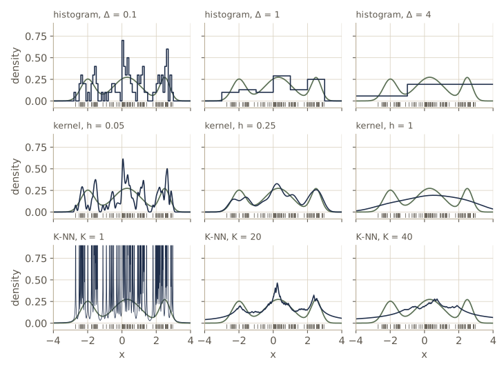
The same idea classifies. Draw the sphere around a new \(\mathbf{x}\) containing \(K\) points regardless of class, and suppose \(K_k\) of them belong to class \(\mathcal{C}_k\), which has \(N_k\) points in total. The density estimates \(p(\mathbf{x} \mid \mathcal{C}_k) = K_k/(N_k V)\), \(p(\mathbf{x}) = K/(NV)\), and priors \(p(\mathcal{C}_k) = N_k/N\) combine through Bayes’ theorem into
\[p(\mathcal{C}_k \mid \mathbf{x}) = \frac{K_k}{K}.\]To minimize misclassification we pick the class with the most representatives among the \(K\) nearest neighbors. With \(K = 1\) this is the nearest-neighbor rule, and a classical result of Cover and Hart shows that, as \(N \to \infty\), its error rate is at most twice the minimum achievable one. We try it on two interleaved half-moons.
def knn_classify(Xq, Xtr, ttr, K, n_classes):
    """p(C_k | x) = K_k / K: class fractions among the K nearest training points."""
    d2 = np.sum(Xq ** 2, 1)[:, None] - 2 * Xq @ Xtr.T + np.sum(Xtr ** 2, 1)[None, :]
    nn = np.argpartition(d2, K - 1, axis=1)[:, :K]
    return np.stack([np.mean(ttr[nn] == k, axis=1) for k in range(n_classes)], axis=1)

def two_moons(n, rng, noise=0.25):
    t = rng.integers(0, 2, n)
    ang = rng.uniform(0, np.pi, n)
    X = np.where(t[:, None] == 0,
                 np.column_stack([np.cos(ang), np.sin(ang)]),
                 np.column_stack([1 - np.cos(ang), 0.5 - np.sin(ang)]))
    return X + noise * rng.normal(size=(n, 2)), t

rng_c = np.random.default_rng(5)
Xc_tr, tc_tr = two_moons(300, rng_c)
Xc_te, tc_te = two_moons(2000, rng_c)
for K in (1, 5, 15, 51, 151):
    probs = knn_classify(Xc_te, Xc_tr, tc_tr, K, 2)
    print(f"K = {K:3d}: test accuracy {np.mean(np.argmax(probs, axis=1) == tc_te):.3f}")
K =   1: test accuracy 0.920
K =   5: test accuracy 0.932
K =  15: test accuracy 0.948
K =  51: test accuracy 0.939
K = 151: test accuracy 0.845
The familiar pattern again: \(K = 1\) follows the noise in individual training points, \(K = 151\) (half the training set) averages over both moons, and a moderate \(K\) does best.
Nearest neighbors and kernels scale better with dimension than histograms, but they still suffer in high dimensions, for a reason that is easy to demonstrate. For random points in a \(D\)-dimensional cube, compare the distance from a query to its nearest and its farthest neighbor:
rng_q = np.random.default_rng(8)
for D in (1, 2, 10, 100, 1000):
    Xd = rng_q.random((1000, D))
    q = rng_q.random((1, D))
    d = np.sqrt(np.sum((Xd - q) ** 2, axis=1))
    print(f"D = {D:4d}: nearest / farthest distance = {d.min() / d.max():.3f}")
D =    1: nearest / farthest distance = 0.001
D =    2: nearest / farthest distance = 0.011
D =   10: nearest / farthest distance = 0.246
D =  100: nearest / farthest distance = 0.701
D = 1000: nearest / farthest distance = 0.882
In high dimensions all 1000 points are nearly the same distance away, so “the neighborhood of \(\mathbf{x}\)” stops meaning much. Real data such as images are not uniform in their cube and behave better, but the effect is why neither method is used as a density model for raw images.
Watch out. Kernel and nearest-neighbor methods keep the entire training set, and every prediction costs a pass over it (tree-based and approximate neighbor search reduce this but do not remove it). Parametric models compress the data into a fixed set of parameters but commit to a shape. Deep networks aim for both: a large but fixed number of parameters, and a flexible shape learned from data.
Summary
| Distribution or method | What it models | Key formula or property |
|---|---|---|
| Bernoulli | one binary variable; sigmoid output | \(\mu_{\mathrm{ML}} = m/N\); loss \(\ln(1 + e^{a}) - ta\), gradient \(y - t\) |
| Binomial | number of ones in \(N\) trials | mean \(N\mu\), variance \(N\mu(1 - \mu)\) |
| Categorical / multinomial | one of \(K\) states; softmax output | \(\mu_k^{\mathrm{ML}} = m_k/N\); gradient in logits \(m_k - N\mu_k\) |
| Multivariate Gaussian | continuous vectors; regression output | ellipsoids along eigenvectors; \(D(D + 3)/2\) parameters |
| Conditional and marginal | parts of a joint Gaussian | \(\boldsymbol{\mu}_{a \mid b} = \boldsymbol{\mu}_a + \boldsymbol{\Sigma}_{ab}\boldsymbol{\Sigma}_{bb}^{-1}(\mathbf{x}_b - \boldsymbol{\mu}_b)\); \(p(\mathbf{x}_a) = \mathcal{N}(\boldsymbol{\mu}_a, \boldsymbol{\Sigma}_{aa})\) |
| Linear-Gaussian Bayes | hidden \(\mathbf{x}\), measurement \(\mathbf{y} = \mathbf{A}\mathbf{x} + \mathbf{b} +\) noise | posterior precision \(\boldsymbol{\Lambda} + \mathbf{A}^{\mathrm{T}}\mathbf{L}\mathbf{A}\) |
| Gaussian ML | fit from data | sample mean; \(\mathbb{E}[\boldsymbol{\Sigma}_{\mathrm{ML}}] = \frac{N-1}{N}\boldsymbol{\Sigma}\) |
| Sequential estimate | streaming data | \(\mu^{(N)} = \mu^{(N-1)} + \eta_N(x_N - \mu^{(N-1)})\) |
| Gaussian mixture | multimodal densities; MDN outputs | \(\ln\sum_k\pi_k\mathcal{N}_k\) by log-sum-exp; responsibilities \(\gamma_k\) |
| Von Mises | angles | \(\theta_0^{\mathrm{ML}}\) = circular mean; \(A(m_{\mathrm{ML}}) = \bar{r}\) |
| Exponential family | all of the above except mixtures | \(-\nabla\ln g = \mathbb{E}[\mathbf{u}]\); ML = moment matching, concave in \(\boldsymbol{\eta}\) |
| Histogram, kernel, K-NN | densities of any shape | \(p \approx K/(NV)\); one smoothing parameter; cost grows with \(N\) |
Ideas to carry forward:
- A network’s output layer is a distribution from this module with its parameters computed by the network: sigmoid for Bernoulli, softmax for categorical, identity for a Gaussian mean. Its loss is the negative log-likelihood, and its logits are natural parameters, which is why the gradient at the output is always prediction minus target.
- Gaussians are closed under conditioning, marginalizing, and linear-Gaussian Bayes, and the answers need only linear algebra. Much of the probabilistic machinery in the second half of the course (latent variables, diffusion) rests on these three results.
- Work in log space: log-sigmoid, log-softmax, Cholesky log-determinants, and log-sum-exp for mixtures. The naive versions fail exactly where training pushes the model, on confident predictions and on points far from the data.
- Every density estimator has a smoothing knob (degree, bandwidth, \(K\), number of components) that trades noise against bias, and it should be chosen on held-out data, with a properly normalized model.
Exercises
- Show that the Bernoulli distribution is normalized and has mean \(\mu\) and variance \(\mu(1 - \mu)\), and that its entropy is \(-\mu\ln\mu - (1 - \mu)\ln(1 - \mu)\). For which \(\mu\) is the entropy largest? Plot it and compare with the binary cross-entropy of a constant prediction \(y = \mu\) on labels drawn with probability \(\mu\).
- Derive the gradient \(\partial/\partial\eta_k\) of \(\sum_j m_j\ln\operatorname{softmax}(\boldsymbol{\eta})_j\), and show that the Hessian is \(-N(\operatorname{diag}(\boldsymbol{\mu}) - \boldsymbol{\mu}\boldsymbol{\mu}^{\mathrm{T}})\). Show that this matrix has the vector of all ones in its null space and explain what that has to do with adding a constant to every logit. Replace the gradient ascent in the notes by Newton’s method with the pseudo-inverse of the Hessian and count the iterations it needs.
- Show that if \(\mathbf{x} \sim \mathcal{N}(\boldsymbol{\mu}, \boldsymbol{\Sigma})\) then \(\mathbf{A}\mathbf{x} + \mathbf{b}\) is Gaussian with mean \(\mathbf{A}\boldsymbol{\mu} + \mathbf{b}\) and covariance \(\mathbf{A}\boldsymbol{\Sigma}\mathbf{A}^{\mathrm{T}}\). Use this to explain why
gaussian_sampleis correct, and check numerically that sampling with the symmetric square root \(\mathbf{U}\operatorname{diag}(\lambda_i^{1/2})\mathbf{U}^{\mathrm{T}}\) instead of the Cholesky factor gives the same distribution but different individual samples for the same noise. - The KL divergence between \(q = \mathcal{N}(\boldsymbol{\mu}_q, \boldsymbol{\Sigma}_q)\) and \(p = \mathcal{N}(\boldsymbol{\mu}_p, \boldsymbol{\Sigma}_p)\) in \(D\) dimensions is \(\frac{1}{2}\{\ln\frac{\lvert\boldsymbol{\Sigma}_p\rvert}{\lvert\boldsymbol{\Sigma}_q\rvert} - D + \operatorname{Tr}(\boldsymbol{\Sigma}_p^{-1}\boldsymbol{\Sigma}_q) + (\boldsymbol{\mu}_p - \boldsymbol{\mu}_q)^{\mathrm{T}}\boldsymbol{\Sigma}_p^{-1}(\boldsymbol{\mu}_p - \boldsymbol{\mu}_q)\}\). Derive it, implement it with Cholesky factors, and check it against a Monte Carlo average of \(\ln q - \ln p\) under samples from \(q\). (This formula is the regularizer in a variational autoencoder.)
- Partition a Gaussian into three groups \(\mathbf{x}_a, \mathbf{x}_b, \mathbf{x}_c\). Find \(p(\mathbf{x}_a \mid \mathbf{x}_b)\) with \(\mathbf{x}_c\) integrated out, and verify your answer on a four-dimensional example with the numerical-integration approach of the marginal section.
- Use the linear-Gaussian result to show that if \(\mathbf{x}\) and \(\mathbf{z}\) are independent Gaussians, then \(\mathbf{y} = \mathbf{x} + \mathbf{z}\) has mean \(\boldsymbol{\mu}_x + \boldsymbol{\mu}_z\) and covariance \(\boldsymbol{\Sigma}_x + \boldsymbol{\Sigma}_z\). Then take \(x \sim \mathcal{N}(0, 1)\) and \(y = \sqrt{\alpha}\,x + \sqrt{1 - \alpha}\,\epsilon\) with \(\epsilon \sim \mathcal{N}(0, 1)\): find \(p(y)\) and \(p(x \mid y)\), and check them by sampling. (This is one step of a diffusion model’s forward process, module 20.)
- For large \(m\), set \(\xi = m^{1/2}(\theta - \theta_0)\) and expand \(\cos\) to second order to show that the von Mises distribution tends to \(\mathcal{N}(\theta \mid \theta_0, 1/m)\). Use the asymptotic form \(I_0(m) \approx e^m/\sqrt{2\pi m}\) to check the normalizer. Then fit a two-component mixture of von Mises distributions by gradient ascent (softmax weights, log concentrations) to wind data you generate with two prevailing directions.
- Differentiate \(-\nabla\ln g(\boldsymbol{\eta}) = \mathbb{E}[\mathbf{u}(\mathbf{x})]\) once more to show \(-\nabla\nabla\ln g(\boldsymbol{\eta}) = \operatorname{cov}[\mathbf{u}(\mathbf{x})]\). Verify it for the categorical distribution with \(K - 1\) natural parameters by comparing a finite-difference Hessian of \(-\ln g\) with the covariance of the one-hot vector’s first \(K - 1\) entries.
- Write the Poisson distribution \(p(x \mid \lambda) = \lambda^x e^{-\lambda}/x!\) in exponential-family form. What is the natural parameter, and what map takes it back to the mean? Write the negative log-likelihood of a network that predicts a Poisson count from its output activation \(a\), and show that its derivative with respect to \(a\) is again prediction minus target.
- Show that \(\mathbb{E}[\boldsymbol{\Sigma}_{\mathrm{ML}}] = \frac{N-1}{N}\boldsymbol{\Sigma}\) using \(\mathbb{E}[\mathbf{x}_n\mathbf{x}_m^{\mathrm{T}}] = \boldsymbol{\mu}\boldsymbol{\mu}^{\mathrm{T}} + I_{nm}\boldsymbol{\Sigma}\). Then modify the sequential-estimation cell to update a running variance as well as a running mean one point at a time (Welford’s method), and check it against the batch variance.
- Show that the one-dimensional \(K\)-nearest-neighbor density estimate decays like \(K/(2N\lvert x \rvert)\) far from the data, so its integral diverges. Then implement leave-one-out cross-validation for the kernel bandwidth (score each training point under the estimate built from the other \(N - 1\)), and compare the bandwidth it picks with the validation-set choice in the notes.
- In your own words: why is the gradient of a network’s loss with respect to its output logits “prediction minus target” for binary, multiclass, and Gaussian outputs alike? Use the exponential family in your answer, and say what changes when the output is a mixture.
Going further
- Bishop & Bishop, Deep Learning: Foundations and Concepts, chapter 3 — the source for this module. Exercises 3.1–3.4 (discrete distributions), 3.6–3.9 (linear transformations, KL divergence, maximum entropy), 3.12–3.17 (eigenvectors, positive definiteness, parameter counts), 3.18–3.27 (partitioned and linear-Gaussian results), 3.28–3.29 (maximum likelihood and its bias), 3.31–3.34 (the von Mises distribution), 3.35–3.36 (exponential family), and 3.37–3.38 (nonparametric estimates) extend it.
- Intro to ML, module 02 — the full derivations of the partitioned-Gaussian and linear-Gaussian results, plus the Bayesian treatment this module skips (beta, Dirichlet, and normal-gamma priors, Student’s t) and a K-nearest-neighbor classifier study. Intro to ML, module 09 fits Gaussian mixtures with EM.
- Herbert Robbins and Sutton Monro, “A stochastic approximation method”, The Annals of Mathematical Statistics, 1951 — the sequential root-finding scheme behind stochastic gradient methods.
- Thomas M. Cover and Peter E. Hart, “Nearest neighbor pattern classification”, IEEE Transactions on Information Theory, 1967 — the factor-of-two bound for the nearest-neighbor rule.
- Kanti V. Mardia and Peter E. Jupp, Directional Statistics (Wiley, 2000) — distributions on circles and spheres, including von Mises mixtures and the wrapped and projected constructions.
- In this course, the distributions here return as output layers in module 04 and module 05, as mixture density networks in module 06, and as latent-variable models in module 15 and module 16.
These notes follow the chapters of C. M. Bishop and H. Bishop, Deep Learning: Foundations and Concepts (Springer, 2024), the course text, which the authors make free to read online. The explanations, code, figures, and exercises here are written for this course; the book remains the reference, with the full derivations and many more exercises.