CSE 676 · Module 02 · Week 1
Probabilities
The sum and product rules, Bayes' theorem, densities and expectations, the Gaussian and maximum likelihood, change of variables, information theory, and the Bayesian view of parameters.
Companion reading: Bishop & Bishop, Deep Learning: Foundations and Concepts, chapter 2, “Probabilities”
By the end of this module you can
- Derive the sum and product rules from counts, use Bayes’ theorem to turn a test’s error rates into the probability that a positive result is correct, and check the answer by simulation.
- Work with densities, cumulative distributions, expectations, variances, and covariances, and explain why a mini-batch gradient is an unbiased Monte Carlo estimate of the full gradient.
- Fit a Gaussian by maximum likelihood, prove that the maximum likelihood variance is biased by the factor \((N-1)/N\), and show the bias in a simulation.
- Show that least squares is maximum likelihood under Gaussian noise, whatever the function \(y(\mathbf{x}, \mathbf{w})\) is, and turn the fit into a predictive distribution.
- Transform a density through an invertible map with the Jacobian determinant, explain why the mode of a density moves under a nonlinear change of variables, and check a transformed density against samples in one and two dimensions.
- Compute entropy, differential entropy, KL divergence, conditional entropy, and mutual information, prove \(\mathrm{KL}(p \Vert q) \ge 0\) with Jensen’s inequality, and explain why the Gaussian has maximum entropy for a given variance.
- Relate the cross-entropy loss used to train classifiers to KL divergence and maximum likelihood, and describe how forward and reverse KL behave when a simple model is fitted to a two-mode density.
- Read weight decay as a Gaussian prior (MAP estimation), write down the Bayesian predictive distribution, and explain why deep learning mostly works with point estimates.
Contents
- The rules of probability
- Probability densities
- The Gaussian distribution
- Transformation of densities
- Information theory
- Bayesian probabilities
- Summary
- Exercises
- Going further
Module 01 fitted a curve to noisy points by minimizing a sum of squares, watched a flexible model overfit, and tamed it with a penalty on the weights. Those steps were chosen by hand. This module supplies the language that explains them: probability. With it, the sum-of-squares error becomes a likelihood, the penalty becomes a prior, and “how wrong is my model” becomes a KL divergence. Every later module leans on these ideas, from the cross-entropy loss of classifiers to the change-of-variables formula behind normalizing flows.
It helps to separate two sources of uncertainty from the start. Suppose a network estimates the age of a tree from a photograph of its bark. Part of its error comes from having seen only a finite number of labeled trees; more training photographs would shrink it. This is epistemic uncertainty (also called systematic uncertainty): uncertainty from limited knowledge. Another part would remain even with unlimited photographs, because bark alone does not determine age; two trees with identical bark can differ by decades. This is aleatoric uncertainty (intrinsic uncertainty, or noise): it comes from what the input leaves out, and the only cure is a different kind of input, such as a core sample. Probability handles both kinds with the same two rules.
Much of this material also appears in the Intro to ML notes (module 01 and module 02), which go further on several derivations. Here we keep each topic compact, run every result in NumPy, and point out where each idea is used inside neural networks.
The rules of probability
A screening test
We start with a concrete question. A blood test screens for a condition that affects 4 people in 1,000. When someone has the condition, the test comes back positive 92% of the time; this rate is the test’s sensitivity. When someone does not, it still comes back positive 2% of the time, a false positive; the 8% of affected people who test negative are false negatives. Two questions matter to anyone being screened. How likely is a positive result at all? And if my result is positive, how likely is it that I have the condition?
Before answering, we derive the two rules that answer every question of this kind.
The sum and product rules
Take two random variables, quantities whose values vary from trial to trial in a way we cannot predict: \(X\) with possible values \(x_1, \dots, x_L\) and \(Y\) with values \(y_1, \dots, y_M\). Run \(N\) trials and count \(n_{ij}\), the number of trials with \(X = x_i\) and \(Y = y_j\). Let \(c_i = \sum_j n_{ij}\) count the trials with \(X = x_i\) regardless of \(Y\). As \(N \to \infty\), fractions of trials become probabilities:
- the joint probability \(p(X = x_i, Y = y_j) = n_{ij}/N\);
- the marginal probability \(p(X = x_i) = c_i/N\);
- the conditional probability \(p(Y = y_j \mid X = x_i) = n_{ij}/c_i\), the fraction of the \(X = x_i\) trials that also have \(Y = y_j\).
Because \(c_i = \sum_j n_{ij}\), the marginal is a sum of joints. Because \(n_{ij}/N = (n_{ij}/c_i)(c_i/N)\), the joint is a conditional times a marginal. Writing \(p(X)\) for the whole distribution of \(X\), these are the two rules on which everything else rests:
Result. The sum rule and the product rule:
\[p(X) = \sum_{Y} p(X, Y), \qquad\qquad p(X, Y) = p(Y \mid X)\, p(X).\]
Summing out a variable with the sum rule is called marginalizing. Let us build the count table for the screening test by simulating two million people. Let \(C = 1\) mean the person has the condition and \(T = 1\) mean a positive test.
import numpy as np
from scipy import special, stats, optimize

np.set_printoptions(precision=4, suppress=True)
rng = np.random.default_rng(676)

prior, sens, fpr = 0.004, 0.92, 0.02      # p(C=1), p(T=1 | C=1), p(T=1 | C=0)

N_people = 2_000_000
C = rng.random(N_people) < prior                            # who has the condition
T = rng.random(N_people) < np.where(C, sens, fpr)           # each person's test result
counts = np.array([[np.sum(~C & ~T), np.sum(~C & T)],       # n_ij: rows C = 0, 1
                   [np.sum(C & ~T), np.sum(C & T)]])        #       columns T = 0, 1
c_i = counts.sum(axis=1)                                    # people with C = 0 and C = 1
print("counts n_ij:\n", counts)
print("marginal p(C) from counts:", c_i / N_people)
print(f"p(T=1 | C=1) from counts: {counts[1, 1] / c_i[1]:.4f}   (sensitivity {sens})")
print(f"p(T=1 | C=0) from counts: {counts[0, 1] / c_i[0]:.4f}   (false-positive rate {fpr})")
counts n_ij:
 [[1952236   39850]
 [    623    7291]]
marginal p(C) from counts: [0.996 0.004]
p(T=1 | C=1) from counts: 0.9213   (sensitivity 0.92)
p(T=1 | C=0) from counts: 0.0200   (false-positive rate 0.02)
The fractions match the rates we put in, up to sampling noise that shrinks as the population grows.
Bayes’ theorem
The product rule holds in either order, \(p(X, Y) = p(Y \mid X)\,p(X) = p(X \mid Y)\,p(Y)\). Dividing by \(p(X)\) gives Bayes’ theorem,
\[p(Y \mid X) = \frac{p(X \mid Y)\, p(Y)}{p(X)}, \qquad p(X) = \sum_{Y} p(X \mid Y)\, p(Y).\]It reverses a conditional: from the probability of \(X\) given \(Y\), which is often what we know, to the probability of \(Y\) given \(X\), which is often what we want. The denominator comes from the sum and product rules and is the constant that makes the left side sum to one over \(Y\).
The screening test, answered
The sensitivity and false-positive rate are conditionals \(p(T \mid C)\). The first question asks for \(p(T = 1)\), which the sum and product rules give directly:
\[p(T = 1) = p(T = 1 \mid C = 1)\,p(C = 1) + p(T = 1 \mid C = 0)\,p(C = 0) = 0.92 \times 0.004 + 0.02 \times 0.996 = 0.02360.\]The second question asks for \(p(C = 1 \mid T = 1)\), the reverse conditional, which is a job for Bayes’ theorem:
\[p(C = 1 \mid T = 1) = \frac{p(T = 1 \mid C = 1)\,p(C = 1)}{p(T = 1)} = \frac{0.00368}{0.02360} \approx 0.156.\]We compute both from the tables and compare with the simulated population.
p_C = np.array([1 - prior, prior])                  # p(C): index 0 = no condition, 1 = condition
p_T_given_C = np.array([[1 - fpr, fpr],             # rows C = 0, 1; columns T = 0, 1
                        [1 - sens, sens]])

joint = p_T_given_C * p_C[:, None]                  # product rule: p(C, T) = p(T | C) p(C)
p_T = joint.sum(axis=0)                             # sum rule: p(T) = sum over C of p(C, T)
p_C_given_T = joint / p_T                           # Bayes: p(C | T) = p(C, T) / p(T)

print(f"p(T=1)       exact {p_T[1]:.5f}   simulated {T.mean():.5f}")
print(f"p(C=1 | T=1) exact {p_C_given_T[1, 1]:.4f}    simulated {C[T].mean():.4f}")
print(f"p(C=1 | T=0) exact {p_C_given_T[1, 0]:.6f}  simulated {C[~T].mean():.6f}")
p(T=1)       exact 0.02360   simulated 0.02357
p(C=1 | T=1) exact 0.1559    simulated 0.1547
p(C=1 | T=0) exact 0.000328  simulated 0.000319
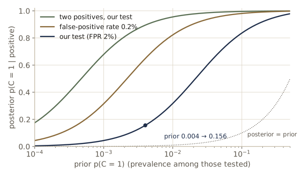
A positive result raises the probability of the condition from 0.4% to about 16%. It does not make the condition likely: roughly five of every six positives are false alarms. A negative result, on the other hand, is very reassuring: the probability falls to about 0.03%.
Prior and posterior probabilities
The screening calculation has a reading that runs through the whole course. Before the test, the best statement we can make about a person is \(p(C)\), the prior probability. After seeing the result we update it to \(p(C \mid T)\), the posterior probability. Bayes’ theorem is the update rule, and the result depends on both ingredients: a test that looks accurate still gives a modest posterior when the prior is small, because the few true positives are outnumbered by false positives from the much larger unaffected group.
Figure 1 shows how strongly the posterior depends on the prior. The same test is far more convincing in a clinic, where the condition is common among the people tested, than in a population-wide screen.
def posterior_positive(prior, sens, fpr):
    """p(C=1 | T=1) by Bayes' theorem."""
    return sens * prior / (sens * prior + fpr * (1 - prior))

for pr in [0.0004, 0.004, 0.04, 0.4]:
    print(f"prior {pr:7.4f}:  posterior after a positive = {posterior_positive(pr, sens, fpr):.4f}")

# a second, independent test: yesterday's posterior is today's prior
post1 = posterior_positive(prior, sens, fpr)
post2 = posterior_positive(post1, sens, fpr)
T2 = rng.random(N_people) < np.where(C, sens, fpr)         # a second, independent test
both = T & T2
print(f"after two positives: {post2:.4f}   simulated {C[both].mean():.4f}")
prior  0.0004:  posterior after a positive = 0.0181
prior  0.0040:  posterior after a positive = 0.1559
prior  0.0400:  posterior after a positive = 0.6571
prior  0.4000:  posterior after a positive = 0.9684
after two positives: 0.8947   simulated 0.8967
The last lines apply Bayes’ theorem twice. If the second test’s errors are independent of the first’s once we know \(C\), the posterior after the first test serves as the prior for the second. Two positives take us from 0.4% to about 89%. This sequential use of Bayes’ theorem, where each posterior becomes the next prior, returns when we learn parameters from data one batch at a time.
Independence
Two variables are independent if their joint distribution factorizes, \(p(X, Y) = p(X)\,p(Y)\). The product rule then gives \(p(Y \mid X) = p(Y)\): learning \(X\) changes nothing about \(Y\). A screening test whose result is independent of the condition is useless, because Bayes’ theorem returns the prior unchanged:
print(f"sens = fpr = 0.3: posterior {posterior_positive(prior, 0.3, 0.3):.4f} prior {prior}")
sens = fpr = 0.3: posterior 0.0040 prior 0.004
The two-test calculation used a weaker property, conditional independence: the test results are dependent (both tend to be positive for affected people), but independent once \(C\) is known, \(p(T_1, T_2 \mid C) = p(T_1 \mid C)\,p(T_2 \mid C)\). Conditional independence is the structure behind the graphical models of module 11. Independence of data points is the assumption behind almost every loss function in this course, as we see next.
Probability densities
For a continuous variable, the probability of any single exact value is zero, so we describe it instead by a probability density \(p(x)\): the probability that \(x\) falls in a small interval \((x, x + \delta x)\) is \(p(x)\,\delta x\) in the limit \(\delta x \to 0\). Probabilities of intervals are integrals,
\[p(x \in (a, b)) = \int_a^b p(x)\, dx, \qquad p(x) \ge 0, \qquad \int_{-\infty}^{\infty} p(x)\, dx = 1 .\]The cumulative distribution function \(P(z) = \int_{-\infty}^{z} p(x)\, dx\) gives the probability that \(x \le z\), and \(P'(x) = p(x)\). For a vector \(\mathbf{x} = (x_1, \dots, x_D)^{\mathrm{T}}\) the joint density \(p(\mathbf{x})\) gives probability \(p(\mathbf{x})\,\delta\mathbf{x}\) to a small volume \(\delta\mathbf{x}\) around \(\mathbf{x}\), and integrates to one over the whole space. The sum and product rules and Bayes’ theorem carry over with integrals in place of sums:
\[p(x) = \int p(x, y)\, dy, \qquad p(x, y) = p(y \mid x)\, p(x), \qquad p(y \mid x) = \frac{p(x \mid y)\, p(y)}{\int p(x \mid y)\, p(y)\, dy}.\]One informal way to see this is to chop each real variable into bins of width \(\Delta\), apply the discrete rules to the bins, and let \(\Delta \to 0\); a rigorous treatment needs measure theory, which we will not need.
Watch out. A density is not a probability, and it can be larger than 1. An exponential density with rate 1.5 has the value 1.5 at \(x = 0\). Only integrals of a density over a region are probabilities.
Example distributions
A constant density over the whole real line cannot be normalized: its integral diverges. A distribution that cannot be normalized is called improper. Restricted to an interval \((c, d)\), a constant becomes the uniform distribution \(p(x) = 1/(d - c)\). Three other simple densities appear often:
- the exponential distribution \(p(x \mid \lambda) = \lambda \exp(-\lambda x)\) for \(x \ge 0\), with rate \(\lambda > 0\);
- the Laplace distribution \(p(x \mid \mu, \gamma) = \frac{1}{2\gamma}\exp\left(-\frac{\lvert x - \mu \rvert}{\gamma}\right)\), an exponential reflected about a location \(\mu\), with scale \(\gamma\);
- the Dirac delta \(\delta(x - \mu)\), zero everywhere except at \(x = \mu\) and integrating to one: an infinitely narrow spike of unit area, which puts all probability on one point.
Deltas let us write a data set \(\mathcal{D} = \{x_1, \dots, x_N\}\) as a distribution. The empirical distribution puts mass \(1/N\) on each observation,
\[p(x \mid \mathcal{D}) = \frac{1}{N} \sum_{n=1}^{N} \delta(x - x_n).\]It is the distribution a model “sees” during training, and we will meet it again when we connect maximum likelihood to the KL divergence. A quick numerical check of the three continuous densities, whose means and variances have known closed forms:
def uniform_pdf(x, c, d):
    return np.where((x > c) & (x < d), 1.0 / (d - c), 0.0)

def exponential_pdf(x, lam):
    return np.where(x >= 0, lam * np.exp(-lam * np.clip(x, 0, None)), 0.0)

def laplace_pdf(x, mu, gamma):
    return np.exp(-np.abs(x - mu) / gamma) / (2 * gamma)

xg = np.linspace(-30, 30, 1_200_001)
cases = [("uniform(0, 2)", uniform_pdf(xg, 0, 2), 1.0, 4 / 12),
         ("exponential(1.5)", exponential_pdf(xg, 1.5), 1 / 1.5, 1 / 1.5 ** 2),
         ("Laplace(0.5, 0.7)", laplace_pdf(xg, 0.5, 0.7), 0.5, 2 * 0.7 ** 2)]
for name, p, mean, var in cases:
    m = np.trapezoid(xg * p, xg)
    v = np.trapezoid((xg - m) ** 2 * p, xg)
    print(f"{name:18s} integral {np.trapezoid(p, xg):.4f}   mean {m:.4f} ({mean:.4f})"
          f"   variance {v:.4f} ({var:.4f})")
uniform(0, 2)      integral 1.0000   mean 1.0000 (1.0000)   variance 0.3333 (0.3333)
exponential(1.5)   integral 1.0000   mean 0.6667 (0.6667)   variance 0.4445 (0.4444)
Laplace(0.5, 0.7)  integral 1.0000   mean 0.5000 (0.5000)   variance 0.9800 (0.9800)
The numbers in parentheses are the closed forms: \((c+d)/2\) and \((d-c)^2/12\) for the uniform, \(1/\lambda\) and \(1/\lambda^2\) for the exponential, \(\mu\) and \(2\gamma^2\) for the Laplace.
Expectations and covariances
The expectation of a function \(f(x)\) is its average under \(p(x)\),
\[\mathbb{E}[f] = \sum_x p(x)\, f(x) \quad \text{(discrete)}, \qquad \mathbb{E}[f] = \int p(x)\, f(x)\, dx \quad \text{(continuous)}.\]Given \(N\) points drawn from \(p(x)\), the expectation under the empirical distribution is the sample average, which approximates the true expectation and becomes exact as \(N \to \infty\):
\[\mathbb{E}[f] \approx \frac{1}{N} \sum_{n=1}^{N} f(x_n).\]A subscript names the variable being averaged: \(\mathbb{E}_x[f(x, y)]\) averages over \(x\) and is a function of \(y\). The conditional expectation \(\mathbb{E}_x[f \mid y] = \int p(x \mid y)\, f(x)\, dx\) averages under a conditional distribution. The variance measures spread around the mean, and expanding the square gives a useful second form:
\[\operatorname{var}[f] = \mathbb{E}\left[ \bigl(f(x) - \mathbb{E}[f(x)]\bigr)^2 \right] = \mathbb{E}[f(x)^2] - \mathbb{E}[f(x)]^2 .\]The covariance of two variables measures how they vary together, \(\operatorname{cov}[x, y] = \mathbb{E}_{x,y}\bigl[\{x - \mathbb{E}[x]\}\{y - \mathbb{E}[y]\}\bigr] = \mathbb{E}_{x,y}[xy] - \mathbb{E}[x]\,\mathbb{E}[y]\), and it is zero when \(x\) and \(y\) are independent. For vectors it is a matrix,
\[\operatorname{cov}[\mathbf{x}, \mathbf{y}] = \mathbb{E}_{\mathbf{x},\mathbf{y}}\left[ \{\mathbf{x} - \mathbb{E}[\mathbf{x}]\}\{\mathbf{y}^{\mathrm{T}} - \mathbb{E}[\mathbf{y}^{\mathrm{T}}]\} \right] = \mathbb{E}_{\mathbf{x},\mathbf{y}}[\mathbf{x}\mathbf{y}^{\mathrm{T}}] - \mathbb{E}[\mathbf{x}]\,\mathbb{E}[\mathbf{y}^{\mathrm{T}}],\]and \(\operatorname{cov}[\mathbf{x}] \equiv \operatorname{cov}[\mathbf{x}, \mathbf{x}]\) is the covariance matrix of the components of \(\mathbf{x}\).
Mini-batches are Monte Carlo estimates. Sample averages are how deep networks are trained. The training error is usually an average of per-example losses, \(E(\mathbf{w}) = \frac{1}{N}\sum_n E_n(\mathbf{w})\), which is an expectation under the empirical distribution. Its gradient is an expectation too. A mini-batch of \(B\) examples drawn at random gives the average of \(B\) per-example gradients, whose expectation over the random draw is exactly the full gradient: it is an unbiased estimate. Its covariance is roughly \(1/B\) times the covariance of a single example’s gradient, so its standard deviation shrinks like \(1/\sqrt{B}\). Module 07 builds stochastic gradient descent on exactly this fact. Here it is for a straight-line model with a squared error.
N = 5_000
x_mb = rng.uniform(-2, 2, N)
t_mb = 1.0 - 0.7 * x_mb + rng.normal(0, 0.5, N)
w = np.array([0.2, 0.3])                        # the current weights (w0, w1)

def per_example_grads(w, x, t):
    """Rows: gradient of E_n = (w0 + w1 x_n - t_n)^2 / 2 with respect to (w0, w1)."""
    r = w[0] + w[1] * x - t
    return np.stack([r, r * x], axis=1)

G = per_example_grads(w, x_mb, t_mb)
g_full = G.mean(axis=0)
Sigma_g = np.cov(G.T, bias=True)                # covariance of one example's gradient
print("full gradient:", g_full)
for B in [10, 100, 1000]:
    idx = np.array([rng.choice(N, B, replace=False) for _ in range(4000)])
    g_batch = G[idx].mean(axis=1)               # 4000 mini-batch gradients
    print(f"B = {B:4d}: mean {g_batch.mean(axis=0)}   std {g_batch.std(axis=0)}   "
          f"formula {np.sqrt(np.diag(Sigma_g) / B)}")
full gradient: [-0.8096  1.3613]
B =   10: mean [-0.8136  1.3577]   std [0.4009 0.5149]   formula [0.4011 0.5188]
B =  100: mean [-0.8141  1.3667]   std [0.1238 0.164 ]   formula [0.1268 0.164 ]
B = 1000: mean [-0.8095  1.3614]   std [0.036  0.0473]   formula [0.0401 0.0519]
The average of the mini-batch gradients matches the full gradient for every batch size, and their standard deviation follows the formula \(\sqrt{\operatorname{diag}(\boldsymbol{\Sigma})/B}\), where \(\boldsymbol{\Sigma}\) is the covariance matrix of a single example’s gradient. (At \(B = 1000\) the spread is a little below the formula because we sample a fifth of the data set without replacement; exercise 2 derives the exact factor.)
The Gaussian distribution
The Gaussian or normal distribution over a real variable \(x\) is
\[\mathcal{N}(x \mid \mu, \sigma^2) = \frac{1}{(2\pi\sigma^2)^{1/2}} \exp\left\{ -\frac{1}{2\sigma^2}(x - \mu)^2 \right\}.\]Its two parameters are the mean \(\mu\) and the variance \(\sigma^2\); \(\sigma\) is the standard deviation, and \(\beta = 1/\sigma^2\) is the precision. The density is positive everywhere and integrates to one (the classic proof squares the integral and switches to polar coordinates). We will see two reasons why the Gaussian is so common: it has the largest entropy for a given variance (later in this module), and sums of many independent variables tend toward it (module 03). The multivariate Gaussian also belongs to module 03.
Mean and variance
The first moment \(\mathbb{E}[x]\) and the second moment \(\mathbb{E}[x^2]\) of the Gaussian are
\[\mathbb{E}[x] = \int \mathcal{N}(x \mid \mu, \sigma^2)\, x\, dx = \mu, \qquad \mathbb{E}[x^2] = \int \mathcal{N}(x \mid \mu, \sigma^2)\, x^2\, dx = \mu^2 + \sigma^2,\]so \(\operatorname{var}[x] = \mathbb{E}[x^2] - \mathbb{E}[x]^2 = \sigma^2\), which justifies the names of the parameters. The first integral follows from the substitution \(z = x - \mu\) and the symmetry of the integrand; the second from differentiating the normalization condition with respect to \(\sigma^2\). The maximum of a density is its mode; for the Gaussian it is at the mean. We check the moments numerically, with a function we reuse all module long.
def gauss_pdf(x, mu, var):
    """N(x | mu, var)."""
    return np.exp(-0.5 * (x - mu) ** 2 / var) / np.sqrt(2 * np.pi * var)

mu0, var0 = -0.4, 1.3 ** 2
p = gauss_pdf(xg, mu0, var0)
print(f"integral {np.trapezoid(p, xg):.6f}   E[x] {np.trapezoid(xg * p, xg):.6f}   "
      f"E[x^2] {np.trapezoid(xg ** 2 * p, xg):.6f}   mu^2 + sigma^2 = {mu0 ** 2 + var0:.6f}")
print(f"mode on the grid: {xg[np.argmax(p)]:.4f}")
integral 1.000000   E[x] -0.400000   E[x^2] 1.850000   mu^2 + sigma^2 = 1.850000
mode on the grid: -0.4000
The likelihood function
Now suppose we observe \(N\) values \(\mathsf{x} = (x_1, \dots, x_N)\) and want to find the Gaussian they came from. Estimating a distribution from a finite sample is called density estimation. On its own the problem has no unique answer, since any density that is positive at the observed points could have produced them; restricting ourselves to Gaussians makes it well posed.
We assume the observations are independent and identically distributed, abbreviated i.i.d.: each is drawn from the same distribution, independently of the others. Independence turns the probability of the whole data set into a product,
\[p(\mathsf{x} \mid \mu, \sigma^2) = \prod_{n=1}^{N} \mathcal{N}(x_n \mid \mu, \sigma^2).\]Viewed as a function of the parameters, with the data held fixed, this is the likelihood function. Maximum likelihood picks the parameters that make the observed data most probable. We maximize the logarithm instead, which has the same maximizer because \(\ln\) is increasing, turns the product into a sum, and avoids a numerical problem we will see in a moment:
\[\ln p(\mathsf{x} \mid \mu, \sigma^2) = -\frac{1}{2\sigma^2} \sum_{n=1}^{N} (x_n - \mu)^2 - \frac{N}{2} \ln \sigma^2 - \frac{N}{2} \ln(2\pi).\]Setting the derivative with respect to \(\mu\) to zero gives \(\sum_n (x_n - \mu) = 0\). Setting the derivative with respect to \(\sigma^2\) to zero gives \(\frac{1}{2\sigma^4}\sum_n (x_n - \mu)^2 = \frac{N}{2\sigma^2}\). Solving the first and substituting into the second:
\[\mu_{\mathrm{ML}} = \frac{1}{N} \sum_{n=1}^{N} x_n, \qquad \sigma^2_{\mathrm{ML}} = \frac{1}{N} \sum_{n=1}^{N} (x_n - \mu_{\mathrm{ML}})^2 .\]These are the sample mean and the sample variance measured about the sample mean. The equation for \(\mu\) does not involve \(\sigma^2\), so we solve for the mean first and then the variance.
def gauss_loglik(x, mu, var):
    """ln p(x | mu, var) for i.i.d. data: a sum of log densities."""
    return np.sum(-0.5 * (x - mu) ** 2 / var - 0.5 * np.log(2 * np.pi * var))

x_obs = rng.normal(2.0, 0.8, size=40)
mu_ml = x_obs.mean()
var_ml = np.mean((x_obs - mu_ml) ** 2)

h = 1e-5                                          # central differences at the maximum
d_mu = (gauss_loglik(x_obs, mu_ml + h, var_ml) - gauss_loglik(x_obs, mu_ml - h, var_ml)) / (2 * h)
d_var = (gauss_loglik(x_obs, mu_ml, var_ml + h) - gauss_loglik(x_obs, mu_ml, var_ml - h)) / (2 * h)
loc, scale = stats.norm.fit(x_obs)                # SciPy's maximum likelihood fit, as a check
print(f"mu_ML {mu_ml:.4f}   sigma2_ML {var_ml:.4f}   (SciPy: {loc:.4f}, {scale ** 2:.4f})")
print(f"derivatives at the maximum: {d_mu:.1e}, {d_var:.1e}")

x_big = rng.normal(2.0, 0.8, size=2000)
print(f"product of 2000 densities: {np.prod(gauss_pdf(x_big, 2.0, 0.64))}")
print(f"sum of 2000 log densities: {gauss_loglik(x_big, 2.0, 0.64):.2f}")
mu_ML 2.0094   sigma2_ML 0.9112   (SciPy: 2.0094, 0.9112)
derivatives at the maximum: 0.0e+00, 1.4e-09
product of 2000 densities: 0.0
sum of 2000 log densities: -2368.53
The last two lines show the numerical reason for logs. Each density value is below one, and the product of 2,000 of them is smaller than the smallest positive double-precision number, so it underflows to zero; the sum of logs is an ordinary number. Deep learning libraries work with log-probabilities throughout for the same reason.
The bias of maximum likelihood
Maximum likelihood underlies most of the losses in this course, so it is worth knowing its flaws. The simplest one shows up with the Gaussian. The estimates \(\mu_{\mathrm{ML}}\) and \(\sigma^2_{\mathrm{ML}}\) are functions of a random data set, so they are random themselves. Suppose the data really come from \(\mathcal{N}(\mu, \sigma^2)\) and we average the estimates over many data sets of size \(N\).
The mean is fine: \(\mathbb{E}[\mu_{\mathrm{ML}}] = \frac{1}{N}\sum_n \mathbb{E}[x_n] = \mu\). Independence also gives \(\operatorname{var}[\mu_{\mathrm{ML}}] = \frac{1}{N^2}\sum_n \operatorname{var}[x_n] = \sigma^2/N\). For the variance, write each deviation from the sample mean as a deviation from the true mean minus the error of the sample mean, \(x_n - \mu_{\mathrm{ML}} = (x_n - \mu) - (\mu_{\mathrm{ML}} - \mu)\), and expand the square:
\[\begin{aligned} \sum_{n=1}^{N} (x_n - \mu_{\mathrm{ML}})^2 &= \sum_{n=1}^{N} (x_n - \mu)^2 - 2(\mu_{\mathrm{ML}} - \mu)\sum_{n=1}^{N} (x_n - \mu) + N(\mu_{\mathrm{ML}} - \mu)^2 \\ &= \sum_{n=1}^{N} (x_n - \mu)^2 - N(\mu_{\mathrm{ML}} - \mu)^2 , \end{aligned}\]where the second line uses \(\sum_n (x_n - \mu) = N(\mu_{\mathrm{ML}} - \mu)\). Now take expectations. Each \((x_n - \mu)^2\) has expectation \(\sigma^2\), and \((\mu_{\mathrm{ML}} - \mu)^2\) has expectation \(\operatorname{var}[\mu_{\mathrm{ML}}] = \sigma^2/N\). Dividing by \(N\):
Result. For i.i.d. Gaussian data,
\[\mathbb{E}[\mu_{\mathrm{ML}}] = \mu, \qquad \mathbb{E}[\sigma^2_{\mathrm{ML}}] = \frac{1}{N}\left(N\sigma^2 - \sigma^2\right) = \frac{N-1}{N}\,\sigma^2 .\]
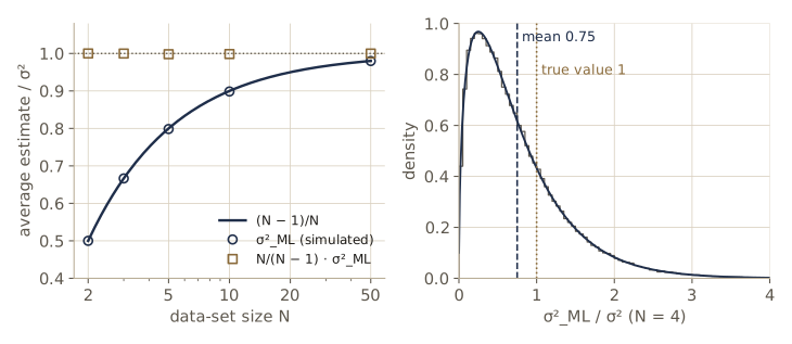
On average, maximum likelihood underestimates the variance. An estimator whose average differs from the true value is biased. The derivation shows exactly where the bias comes from: the spread is measured around \(\mu_{\mathrm{ML}}\), which was fitted to these same points and therefore sits closer to them than the true mean does, by an amount whose square averages \(\sigma^2/N\). If we knew the true mean and used \(\widehat{\sigma}^2 = \frac{1}{N}\sum_n (x_n - \mu)^2\), there would be no bias, since \(\mathbb{E}[\widehat{\sigma}^2] = \sigma^2\). We do not know it, but the result tells us how to correct the estimate: the rescaled estimator
\[\widetilde{\sigma}^2 = \frac{N}{N-1}\,\sigma^2_{\mathrm{ML}} = \frac{1}{N-1} \sum_{n=1}^{N} (x_n - \mu_{\mathrm{ML}})^2\]has \(\mathbb{E}[\widetilde{\sigma}^2] = \sigma^2\). A simulation over 200,000 data sets for each of several sizes:
mu_true, var_true = 2.0, 0.64
sim = np.random.default_rng(3)
for N in [2, 3, 5, 10, 50]:
    sets = sim.normal(mu_true, np.sqrt(var_true), size=(200_000, N))
    m_ml = sets.mean(axis=1)
    v_ml = np.mean((sets - m_ml[:, None]) ** 2, axis=1)       # about the sample mean
    v_true_mean = np.mean((sets - mu_true) ** 2, axis=1)      # about the true mean
    print(f"N = {N:2d}: mu_ML {m_ml.mean():.4f}   sigma2_ML {v_ml.mean():.4f} "
          f"(formula {(N - 1) / N * var_true:.4f})   true-mean {v_true_mean.mean():.4f}   "
          f"corrected {(N / (N - 1) * v_ml).mean():.4f}")
N =  2: mu_ML 2.0011   sigma2_ML 0.3200 (formula 0.3200)   true-mean 0.6406   corrected 0.6400
N =  3: mu_ML 2.0000   sigma2_ML 0.4266 (formula 0.4267)   true-mean 0.6396   corrected 0.6399
N =  5: mu_ML 1.9982   sigma2_ML 0.5110 (formula 0.5120)   true-mean 0.6389   corrected 0.6387
N = 10: mu_ML 1.9997   sigma2_ML 0.5751 (formula 0.5760)   true-mean 0.6394   corrected 0.6390
N = 50: mu_ML 2.0000   sigma2_ML 0.6271 (formula 0.6272)   true-mean 0.6398   corrected 0.6399
Each line gives the averages over data sets of \(\mu_{\mathrm{ML}}\), of \(\sigma^2_{\mathrm{ML}}\) (with the formula \(\frac{N-1}{N}\sigma^2\) beside it), of \(\widehat{\sigma}^2\) computed with the true mean, and of the corrected \(\widetilde{\sigma}^2\). The last two sit at \(\sigma^2 = 0.64\) for every \(N\). With two points, maximum likelihood reports half the true variance on average; with fifty, the shortfall is 2%. Figure 2 shows the same numbers as a curve, together with the whole distribution of \(\sigma^2_{\mathrm{ML}}\) for data sets of four points.
Note. For a single Gaussian the bias is harmless unless \(N\) is tiny. It matters because it is the simplest case of a general pattern: maximum likelihood tunes the parameters to the particular sample, so the fitted model looks better on that sample than it really is. With one extra parameter (the mean) the effect is a factor \((N-1)/N\); with the millions of parameters of a neural network it becomes overfitting, and no simple correction factor exists. Regularization, held-out data, and the Bayesian ideas at the end of this module are the remedies.
Linear regression as maximum likelihood
The same reasoning explains the sum-of-squares error of module 01. We want to predict a target \(t\) from an input \(x\), and we express our uncertainty about \(t\) with a Gaussian centered on a model’s prediction:
\[p(t \mid x, \mathbf{w}, \sigma^2) = \mathcal{N}\bigl(t \mid y(x, \mathbf{w}), \sigma^2\bigr).\]Here \(y(x, \mathbf{w})\) can be a polynomial, a linear model with basis functions, or a deep network; nothing below depends on its form. For i.i.d. training pairs \((x_n, t_n)\) the log-likelihood is
\[\ln p(\mathsf{t} \mid \mathsf{x}, \mathbf{w}, \sigma^2) = -\frac{1}{2\sigma^2} \sum_{n=1}^{N} \bigl\{ y(x_n, \mathbf{w}) - t_n \bigr\}^2 - \frac{N}{2} \ln \sigma^2 - \frac{N}{2} \ln(2\pi).\]To maximize over \(\mathbf{w}\) we can drop the last two terms, which do not depend on \(\mathbf{w}\), and the positive factor \(1/\sigma^2\), which does not move the maximum. Flipping the sign turns maximization into minimization of
\[E(\mathbf{w}) = \frac{1}{2} \sum_{n=1}^{N} \bigl\{ y(x_n, \mathbf{w}) - t_n \bigr\}^2 .\]Result. Minimizing the sum-of-squares error is maximum likelihood under additive Gaussian noise. The negative log-likelihood is the error function, up to a scale and a constant: \(-\ln p(\mathsf{t} \mid \mathsf{x}, \mathbf{w}, \sigma^2) = E(\mathbf{w})/\sigma^2 + \frac{N}{2}\ln(2\pi\sigma^2)\).
This is the pattern for every loss in the course. Choose a distribution for the target given the network’s output, and the negative log-likelihood is the loss: Gaussian targets give squared error (module 04), Bernoulli and categorical targets give the cross-entropy losses of modules 05 and 06, and a network can even predict \(\sigma^2\) as a second output when the noise level varies with \(x\) (exercise 4).
Once \(\mathbf{w}_{\mathrm{ML}}\) is found, maximizing over \(\sigma^2\) gives the mean squared residual,
\[\sigma^2_{\mathrm{ML}} = \frac{1}{N} \sum_{n=1}^{N} \bigl\{ y(x_n, \mathbf{w}_{\mathrm{ML}}) - t_n \bigr\}^2 ,\]and together they give a predictive distribution, a full distribution over the target for a new input rather than a single number: \(p(t \mid x, \mathbf{w}_{\mathrm{ML}}, \sigma^2_{\mathrm{ML}}) = \mathcal{N}\bigl(t \mid y(x, \mathbf{w}_{\mathrm{ML}}), \sigma^2_{\mathrm{ML}}\bigr)\). We fit a cubic polynomial to 30 noisy points and check each claim.
def f_true(x):
    return 0.8 * np.sin(2.5 * x) + 0.3 * x

def design(x, M):
    """Polynomial features 1, x, ..., x^M as an (N, M+1) matrix."""
    return x[:, None] ** np.arange(M + 1)

sigma_noise = 0.15
x_tr = rng.uniform(-1.2, 1.2, 30)
t_tr = f_true(x_tr) + rng.normal(0, sigma_noise, 30)
x_te = rng.uniform(-1.2, 1.2, 2000)
t_te = f_true(x_te) + rng.normal(0, sigma_noise, 2000)

Phi = design(x_tr, 3)
w_ml = np.linalg.lstsq(Phi, t_tr, rcond=None)[0]         # least squares = maximum likelihood
var_ml_reg = np.mean((Phi @ w_ml - t_tr) ** 2)

def neg_log_lik(w, var):
    r = Phi @ w - t_tr
    return 0.5 * r @ r / var + 0.5 * len(t_tr) * np.log(2 * np.pi * var)

E = 0.5 * np.sum((Phi @ w_ml - t_tr) ** 2)
print("w_ML:", w_ml)
print(f"NLL {neg_log_lik(w_ml, var_ml_reg):.4f} = E/sigma^2 + (N/2) ln(2 pi sigma^2) = "
      f"{E / var_ml_reg + 15 * np.log(2 * np.pi * var_ml_reg):.4f}")
w_other = w_ml + np.array([0.0, 0.05, 0.0, 0.0])
print(f"a nearby w has higher NLL: {neg_log_lik(w_other, var_ml_reg):.4f}")
print(f"sigma_ML {np.sqrt(var_ml_reg):.4f}   (true noise s.d. {sigma_noise})")
inside = np.abs(t_te - design(x_te, 3) @ w_ml) < 1.96 * np.sqrt(var_ml_reg)
print(f"test targets inside the 95% predictive interval: {inside.mean():.1%}")
w_ML: [ 0.0216  1.9914 -0.1193 -1.2481]
NLL -14.1597 = E/sigma^2 + (N/2) ln(2 pi sigma^2) = -14.1597
a nearby w has higher NLL: -13.3500
sigma_ML 0.1509   (true noise s.d. 0.15)
test targets inside the 95% predictive interval: 91.0%
The noise estimate is close to the true 0.15, but the 95% predictive interval covers only 91% of new targets. Two things we have already met explain the shortfall. The residuals are measured about a curve fitted to these same 30 points, so, like the Gaussian variance, they understate the noise a new point will see. And the plug-in predictive distribution treats \(\mathbf{w}_{\mathrm{ML}}\) as exact, ignoring our uncertainty about the weights themselves; the Bayesian predictive distribution at the end of the module adds it back.
Transformation of densities
One variable
Densities behave differently from ordinary functions when we change variables, and this difference is the foundation of the normalizing flows in module 18. Suppose \(x = g(y)\) for an invertible, differentiable \(g\). An ordinary function \(f(x)\) becomes \(\widetilde{f}(y) = f(g(y))\): we just look up the old value. A density must instead preserve probability. The probability that \(x\) falls in a small interval of length \(\delta x\) is the probability that \(y\) falls in the corresponding interval of length \(\delta y\), so \(p_x(x)\,\lvert\delta x\rvert \approx p_y(y)\,\lvert\delta y\rvert\). Letting the intervals shrink,
\[p_y(y) = p_x(x) \left\lvert \frac{dx}{dy} \right\rvert = p_x\bigl(g(y)\bigr)\, \lvert g'(y) \rvert .\]The absolute value is there because \(g\) may be decreasing, while a ratio of lengths is always positive. The factor \(\lvert g'(y) \rvert\) records how much the map stretches or squeezes space: where \(g\) squeezes a long stretch of \(x\) into a short stretch of \(y\), the density of \(y\) piles up.
The mode moves. For an ordinary function, the maximum of \(\widetilde{f}\) sits at the \(\widehat{y}\) with \(g(\widehat{y}) = \widehat{x}\), because \(\widetilde{f}'(y) = f'(g(y))\,g'(y)\) vanishes wherever \(f'\) does. For a density the extra factor spoils this. Take \(g\) increasing, so \(p_y(y) = p_x(g(y))\,g'(y)\), and differentiate:
\[p_y'(y) = p_x'\bigl(g(y)\bigr)\, g'(y)^2 + p_x\bigl(g(y)\bigr)\, g''(y).\]At the point with \(g(\widehat{y}) = \widehat{x}\) the first term vanishes, but the second does not unless \(g''(\widehat{y}) = 0\). So for a nonlinear \(g\) the mode of \(p_y\) is generally not the image of the mode of \(p_x\); only linear maps, with \(g'' = 0\), preserve it. A “most probable value” depends on the variable we choose to describe it in. We return to this when we meet MAP estimates at the end of the module.
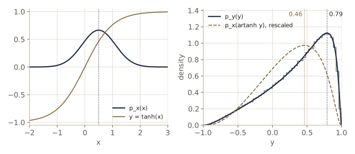
Here is an example that shows up in practice. Some reinforcement-learning methods produce bounded actions by passing a Gaussian through \(\tanh\), and must include exactly this correction when they compute the log-probability of an action. Let \(x \sim \mathcal{N}(0.5, 0.6^2)\) and \(y = \tanh(x)\), so \(x = g(y) = \operatorname{artanh}(y)\) and \(g'(y) = 1/(1 - y^2)\):
\[p_y(y) = \frac{\mathcal{N}\bigl(\operatorname{artanh}(y) \mid \mu, \sigma^2\bigr)}{1 - y^2}, \qquad -1 < y < 1 .\]Setting the derivative of \(\ln p_y\) to zero and writing \(u = \operatorname{artanh}(y)\) gives the condition \(u - \mu = 2\sigma^2 \tanh(u)\) for the mode, whose solution lies well to the right of \(u = \mu\).
mu_x, sd_x = 0.5, 0.6

def p_y_tanh(y):
    """Density of y = tanh(x) for x ~ N(mu_x, sd_x^2): p_x(g(y)) |g'(y)|, g = artanh."""
    return gauss_pdf(np.arctanh(y), mu_x, sd_x ** 2) / (1 - y ** 2)

yg = np.linspace(-1 + 1e-9, 1 - 1e-9, 400_001)
py = p_y_tanh(yg)
naive = gauss_pdf(np.arctanh(yg), mu_x, sd_x ** 2)          # p_x(g(y)): treated as a function
u_hat = optimize.brentq(lambda u: u - mu_x - 2 * sd_x ** 2 * np.tanh(u), -5, 5)
print(f"integral of p_y: {np.trapezoid(py, yg):.5f}")
print(f"tanh(mode of p_x) = tanh({mu_x}) = {np.tanh(mu_x):.4f};  "
      f"max of p_x(g(y)) on the grid: {yg[np.argmax(naive)]:.4f}")
print(f"mode of p_y on the grid: {yg[np.argmax(py)]:.4f};  from u - mu = 2 sigma^2 tanh(u): "
      f"{np.tanh(u_hat):.4f}")

y_samples = np.tanh(rng.normal(mu_x, sd_x, 200_000))
hist, edges = np.histogram(y_samples, bins=50, range=(-1, 1), density=True)
mids = 0.5 * (edges[:-1] + edges[1:])
print(f"largest gap between histogram and p_y: {np.max(np.abs(hist - p_y_tanh(mids))):.3f}"
      f"   (peak of p_y {py.max():.3f})")
integral of p_y: 1.00000
tanh(mode of p_x) = tanh(0.5) = 0.4621;  max of p_x(g(y)) on the grid: 0.4621
mode of p_y on the grid: 0.7886;  from u - mu = 2 sigma^2 tanh(u): 0.7886
largest gap between histogram and p_y: 0.022   (peak of p_y 1.124)
The function \(p_x(g(y))\) peaks at \(\tanh(0.5) = 0.46\), as an ordinary function should; the density \(p_y\) peaks near 0.79, and the histogram of transformed samples agrees with the density, not with the function. The squeezing near \(\pm 1\) is what pushes mass outward (figure 3).
Any density from a simple one. Run the formula the other way and it becomes a way to make samples. If \(u\) is uniform on \((0, 1)\) and \(P\) is a cumulative distribution function with inverse \(P^{-1}\), then \(y = P^{-1}(u)\) has density \(P'(y) = p(y)\): the change of variables multiplies the uniform density 1 by \(\lvert du/dy \rvert = P'(y)\). So every density on the real line can be produced by pushing a fixed simple density through a monotonic function. For the exponential, \(P(y) = 1 - e^{-\lambda y}\) and \(y = -\ln(1 - u)/\lambda\).
lam = 1.5
u = rng.random(100_000)
y_exp = -np.log(1 - u) / lam                        # inverse CDF of the exponential
ks = stats.kstest(y_exp, stats.expon(scale=1 / lam).cdf)
print(f"mean {y_exp.mean():.4f} (1/lambda = {1 / lam:.4f})   "
      f"Kolmogorov-Smirnov distance to the exponential CDF: {ks.statistic:.4f}")
mean 0.6641 (1/lambda = 0.6667) Kolmogorov-Smirnov distance to the exponential CDF: 0.0026
This idea, a simple base density pushed through a learned invertible function, is what a normalizing flow is. Generative adversarial networks, variational autoencoders, and diffusion models (modules 17, 19, 20) also generate data by transforming simple noise, even when they cannot evaluate the resulting density.
Several variables
For a vector \(\mathbf{x} = (x_1, \dots, x_D)^{\mathrm{T}}\) and an invertible map \(\mathbf{x} = \mathbf{g}(\mathbf{y})\) between spaces of the same dimension \(D\), the derivative becomes the Jacobian matrix \(\mathbf{J}\) with elements \(J_{ij} = \partial g_i / \partial y_j\), and the length ratio becomes a volume ratio:
\[p_{\mathbf{y}}(\mathbf{y}) = p_{\mathbf{x}}\bigl(\mathbf{g}(\mathbf{y})\bigr)\, \bigl\lvert \det \mathbf{J} \bigr\rvert, \qquad \mathbf{J} = \begin{pmatrix} \partial g_1/\partial y_1 & \cdots & \partial g_1/\partial y_D \\ \vdots & \ddots & \vdots \\ \partial g_D/\partial y_1 & \cdots & \partial g_D/\partial y_D \end{pmatrix}.\]Near a point, the map acts like the linear map \(\mathbf{J}\), which sends a small box of volume \(\delta\mathbf{y}\) to a parallelepiped of volume \(\lvert\det\mathbf{J}\rvert\,\delta\mathbf{y}\) in \(\mathbf{x}\)-space. The box and its image hold the same probability, which gives the formula; it is the same Jacobian factor that appears when changing variables in a multiple integral.
In \(D\) dimensions a determinant costs \(O(D^3)\) operations in general, which is far too slow inside a model with thousands of dimensions. Flows therefore use maps whose Jacobian is triangular, so that the determinant is the product of the diagonal. The simplest example is a coupling transformation in two dimensions: leave \(x_1\) alone, and scale and shift \(x_2\) by amounts that depend on \(x_1\),
\[y_1 = x_1, \qquad y_2 = x_2\, e^{s(x_1)} + b(x_1).\]The inverse is \(x_1 = y_1\), \(x_2 = \bigl(y_2 - b(y_1)\bigr)e^{-s(y_1)}\), whatever the functions \(s\) and \(b\) are (in a flow they are neural networks). Its Jacobian is lower triangular with diagonal \((1, e^{-s(y_1)})\), so \(\det \mathbf{J} = e^{-s(y_1)}\) and
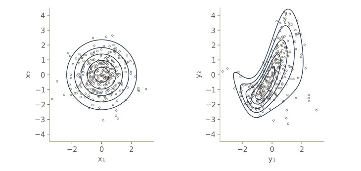
\[\ln p_{\mathbf{y}}(\mathbf{y}) = \ln p_{\mathbf{x}}\bigl(\mathbf{g}(\mathbf{y})\bigr) - s(y_1).\]We take a standard Gaussian for \(\mathbf{x}\), fixed choices \(s(x_1) = 0.6\tanh(x_1)\) and \(b(x_1) = 1.5\sin(1.2\,x_1)\), and check the formula three ways: the Jacobian determinant against finite differences, the density’s integral, and the density against a two-dimensional histogram of transformed samples.
def s_fn(x1):
    return 0.6 * np.tanh(x1)

def b_fn(x1):
    return 1.5 * np.sin(1.2 * x1)

def coupling_forward(X):
    """x -> y: y1 = x1, y2 = x2 exp(s(x1)) + b(x1). X has shape (N, 2)."""
    return np.stack([X[:, 0], X[:, 1] * np.exp(s_fn(X[:, 0])) + b_fn(X[:, 0])], axis=1)

def coupling_inverse(Y):
    """y -> x = g(y)."""
    return np.stack([Y[:, 0], (Y[:, 1] - b_fn(Y[:, 0])) * np.exp(-s_fn(Y[:, 0]))], axis=1)

def log_p_y(Y):
    """ln p_y(y) = ln N(g(y) | 0, I) - s(y1)."""
    X = coupling_inverse(Y)
    return -0.5 * np.sum(X ** 2, axis=1) - np.log(2 * np.pi) - s_fn(Y[:, 0])

y0 = np.array([[0.7, -0.4]])                        # finite-difference Jacobian of g at one point
h = 1e-6
J = np.column_stack([(coupling_inverse(y0 + h * e) - coupling_inverse(y0 - h * e))[0] / (2 * h)
                     for e in np.eye(2)])
print("J at y = (0.7, -0.4):\n", J)
print(f"det J {np.linalg.det(J):.6f}   exp(-s(y1)) {np.exp(-s_fn(0.7)):.6f}")

g1 = np.linspace(-6, 6, 601)                        # integrate p_y over a grid
Y1, Y2 = np.meshgrid(g1, g1, indexing="ij")
P_grid = np.exp(log_p_y(np.column_stack([Y1.ravel(), Y2.ravel()]))).reshape(Y1.shape)
print(f"integral of p_y over the grid: {np.trapezoid(np.trapezoid(P_grid, g1), g1):.5f}")

Y_s = coupling_forward(rng.normal(size=(400_000, 2)))
H2, e1, e2 = np.histogram2d(Y_s[:, 0], Y_s[:, 1], bins=24, range=[[-3, 3], [-3, 3]], density=True)
c1, c2 = np.meshgrid(0.5 * (e1[:-1] + e1[1:]), 0.5 * (e2[:-1] + e2[1:]), indexing="ij")
P_c = np.exp(log_p_y(np.column_stack([c1.ravel(), c2.ravel()]))).reshape(c1.shape)
H2 *= np.mean((np.abs(Y_s) < 3).all(axis=1))        # histogram normalized over the whole plane
print(f"largest gap between the 2-D histogram and p_y: {np.max(np.abs(H2 - P_c)):.4f}"
      f"   (peak of p_y {P_grid.max():.4f})")
J at y = (0.7, -0.4):
 [[ 1.      0.    ]
 [-0.434   0.6959]]
det J 0.695850   exp(-s(y1)) 0.695850
integral of p_y over the grid: 0.99942
largest gap between the 2-D histogram and p_y: 0.0057   (peak of p_y 0.1854)
The determinant from finite differences matches \(e^{-s(y_1)}\), the density integrates to one (up to the little mass outside the grid), and the histogram agrees with the formula to within what we expect from sampling noise and from evaluating the density only at cell centers. Figure 4 shows what the map does: the round Gaussian is bent into a curved band, stretched where \(s > 0\) and squeezed where \(s < 0\).
Information theory
Information theory measures how much information a random quantity carries. It supplies the losses used to train classifiers and the divergences used to compare distributions, both of which recur in almost every later module. The Intro to ML notes treat it at more length (module 01, “Information theory”).
Entropy
How much information do we gain when we learn the value of a discrete variable \(x\)? A rare outcome surprises us more than a common one, and for two independent variables the information should add, while their probabilities multiply. The logarithm is the function that turns products into sums (exercise 2.21 of Bishop & Bishop shows it is the only reasonable choice), so we define the information content of an outcome as
\[h(x) = -\log_2 p(x),\]measured in bits. It is zero for a certain event and grows as the probability shrinks. Its average over the distribution is the entropy,
\[\mathrm{H}[x] = -\sum_x p(x) \log_2 p(x),\]with the convention \(0 \log 0 = 0\) (the limit of \(\epsilon \ln \epsilon\) as \(\epsilon \to 0\)).
Entropy has a concrete meaning: it is the average number of bits needed to transmit the value of \(x\). Take a variable with five states \(\{a, b, c, d, e\}\) and probabilities \(\left(\tfrac12, \tfrac14, \tfrac18, \tfrac1{16}, \tfrac1{16}\right)\). A fixed-length code needs 3 bits per symbol. A code that gives short strings to common states, 0, 10, 110, 1110, 1111, averages fewer, and because no code string is the beginning of another, a concatenated message decodes without separators. Shannon’s noiseless coding theorem says that no code can average fewer bits than the entropy; this code reaches it.
def entropy(p, base=np.e):
    """H[p] = -sum p ln p (nats), with 0 ln 0 = 0; base=2 gives bits."""
    p = np.asarray(p, dtype=float)
    nz = p > 0
    return -np.sum(p[nz] * np.log(p[nz])) / np.log(base)

p5 = np.array([1 / 2, 1 / 4, 1 / 8, 1 / 16, 1 / 16])
code = ["0", "10", "110", "1110", "1111"]
avg_len = sum(pk * len(ck) for pk, ck in zip(p5, code))
print(f"entropy {entropy(p5, 2):.4f} bits   average code length {avg_len:.4f} bits")
print(f"uniform over 5 states: {entropy(np.full(5, 0.2), 2):.4f} bits = log2(5)")

bins = np.arange(20)                                # 20 states; a narrow and a broad distribution
for width in [1.0, 4.0]:
    q = np.exp(-0.5 * ((bins - 9.5) / width) ** 2)
    q /= q.sum()
    print(f"20 states, width {width}: H = {entropy(q):.4f} nats")
print(f"20 states, uniform:   H = {entropy(np.full(20, 0.05)):.4f} nats = ln 20")
entropy 1.8750 bits   average code length 1.8750 bits
uniform over 5 states: 2.3219 bits = log2(5)
20 states, width 1.0: H = 1.4189 nats
20 states, width 4.0: H = 2.7490 nats
20 states, uniform:   H = 2.9957 nats = ln 20
From here on we use natural logarithms, so entropy is measured in nats; one nat is \(1/\ln 2 \approx 1.44\) bits. The last three lines show the general trend: a distribution concentrated on a few states has low entropy, a spread-out one has high entropy, and the uniform distribution has the most.
That last claim follows from a short constrained maximization. Maximize \(-\sum_i p_i \ln p_i\) subject to \(\sum_i p_i = 1\) with a Lagrange multiplier \(\lambda\) (Bishop & Bishop, Appendix C). The derivative of \(-\sum_i p_i \ln p_i + \lambda\left(\sum_i p_i - 1\right)\) with respect to \(p_i\) is \(-\ln p_i - 1 + \lambda\), which vanishes only when all \(p_i\) are equal, \(p_i = 1/M\) for \(M\) states, with entropy \(\ln M\). The second derivatives form the diagonal matrix with entries \(-1/p_i < 0\), so this is a maximum. The minimum, \(\mathrm{H} = 0\), is attained when one state has probability one.
The physics perspective
Entropy began in physics, and the physics reading gives another intuition. Distribute \(N\) identical objects among bins so that bin \(i\) holds \(n_i\) of them. A particular assignment of objects to bins is a microstate; the list of occupation fractions \(n_i/N\) is a macrostate. The number of microstates that realize a macrostate is the multiplicity
\[W = \frac{N!}{\prod_i n_i!},\]because there are \(N!\) orderings of the objects and reordering within a bin changes nothing. Define the entropy as \(\frac{1}{N}\ln W\). Using Stirling’s approximation \(\ln N! \approx N\ln N - N\) and letting \(N \to \infty\) with the fractions \(p_i = n_i/N\) fixed, \(\frac{1}{N}\ln W \to -\sum_i p_i \ln p_i\). A spread-out macrostate can be realized in vastly more ways than a concentrated one, which is why it has higher entropy. The Intro to ML notes check this limit numerically.
Differential entropy
For a continuous variable, cut the line into bins of width \(\Delta\). By the mean value theorem each bin contains a point \(x_i\) with \(\int_{i\Delta}^{(i+1)\Delta} p(x)\,dx = p(x_i)\Delta\), so the binned variable has probabilities \(p(x_i)\Delta\) and entropy
\[\mathrm{H}_\Delta = -\sum_i p(x_i)\Delta \ln\bigl(p(x_i)\Delta\bigr) = -\sum_i p(x_i)\Delta \ln p(x_i) - \ln \Delta ,\]using \(\sum_i p(x_i)\Delta = 1\). As \(\Delta \to 0\) the first term tends to an integral while \(-\ln\Delta\) grows without bound: describing a real number to infinite precision takes infinitely many bits. Dropping the divergent term defines the differential entropy
\[\mathrm{H}[\mathbf{x}] = -\int p(\mathbf{x}) \ln p(\mathbf{x})\, d\mathbf{x}.\]For the exponential distribution, \(\mathrm{H} = 1 - \ln\lambda\). That is negative once \(\lambda > e\): differential entropy, unlike the discrete kind, can be negative, because a density can be much larger than one.
lam = 2.0
H_exp = 1 - np.log(lam)
for Delta in [0.5, 0.1, 0.01, 0.001]:
    edges_d = np.arange(0, 40 + Delta, Delta)
    probs = np.diff(1 - np.exp(-lam * edges_d))     # exact bin probabilities
    print(f"Delta = {Delta:5}:  H_Delta = {entropy(probs):7.4f}   "
          f"H_Delta + ln Delta = {entropy(probs) + np.log(Delta):.4f}")
print(f"differential entropy 1 - ln(lambda) = {H_exp:.4f};  for lambda = 5: {1 - np.log(5):.4f}")
Delta =   0.5:  H_Delta =  1.0407   H_Delta + ln Delta = 0.3475
Delta =   0.1:  H_Delta =  2.6111   H_Delta + ln Delta = 0.3085
Delta =  0.01:  H_Delta =  4.9120   H_Delta + ln Delta = 0.3069
Delta = 0.001:  H_Delta =  7.2146   H_Delta + ln Delta = 0.3069
differential entropy 1 - ln(lambda) = 0.3069;  for lambda = 5: -0.6094
The binned entropy grows as the bins shrink, while \(\mathrm{H}_\Delta + \ln\Delta\) settles on the differential entropy.
Maximum entropy
Which density has the largest differential entropy? Without constraints the question has no answer (spread the density ever wider), so fix the mean \(\mu\) and the variance \(\sigma^2\) as well as the normalization. With Lagrange multipliers \(\lambda_1, \lambda_2, \lambda_3\) for the three constraints, we maximize the functional
\[-\int p \ln p\, dx + \lambda_1\left(\int p\, dx - 1\right) + \lambda_2\left(\int x\, p\, dx - \mu\right) + \lambda_3\left(\int (x - \mu)^2 p\, dx - \sigma^2\right).\]The calculus of variations (Bishop & Bishop, Appendix B) asks that the derivative of the integrand with respect to \(p(x)\) vanish at every \(x\): \(-\ln p(x) - 1 + \lambda_1 + \lambda_2 x + \lambda_3 (x - \mu)^2 = 0\). So \(\ln p(x)\) is a quadratic in \(x\), and \(p\) is the exponential of a quadratic. Matching the three constraints forces \(\lambda_2 = 0\) and \(\lambda_3 = -1/(2\sigma^2)\), and normalization fixes \(\lambda_1\):
Result. Among all densities with a given mean and variance, the Gaussian \(\mathcal{N}(x \mid \mu, \sigma^2)\) has the largest differential entropy, namely
\[\mathrm{H}[x] = -\mathbb{E}\bigl[\ln \mathcal{N}(x \mid \mu, \sigma^2)\bigr] = \tfrac12 \ln(2\pi\sigma^2) + \frac{\mathbb{E}[(x-\mu)^2]}{2\sigma^2} = \tfrac12\bigl\{1 + \ln(2\pi\sigma^2)\bigr\}.\]
We never imposed \(p \ge 0\); the solution satisfies it anyway. The entropy grows with \(\sigma^2\), and it is negative for \(\sigma^2 < 1/(2\pi e)\). In modeling terms, choosing a Gaussian when all we know is a mean and a variance adds the fewest extra assumptions. A numerical comparison with four other densities of the same variance:
def diff_entropy(p, x):
    """-integral p ln p on a grid (0 ln 0 = 0)."""
    safe = np.where(p > 0, p, 1.0)
    return -np.trapezoid(np.where(p > 0, p * np.log(safe), 0.0), x)

sig = 1.0
s_log = sig * np.sqrt(3) / np.pi                     # logistic scale with variance sig^2
m_mix, v_mix = 0.8, sig ** 2 - 0.8 ** 2              # equal mixture of N(-0.8, v) and N(0.8, v)
dens = {"Gaussian": gauss_pdf(xg, 0, sig ** 2),
        "Laplace": laplace_pdf(xg, 0, sig / np.sqrt(2)),
        "uniform": uniform_pdf(xg, -sig * np.sqrt(3), sig * np.sqrt(3)),
        "logistic": stats.logistic.pdf(xg, scale=s_log),
        "two bumps": 0.5 * gauss_pdf(xg, -m_mix, v_mix) + 0.5 * gauss_pdf(xg, m_mix, v_mix)}
for name, p in dens.items():
    var = np.trapezoid(xg ** 2 * p, xg)
    print(f"{name:10s} variance {var:.4f}   entropy {diff_entropy(p, xg):.4f}")
print(f"formula for the Gaussian: {0.5 * (1 + np.log(2 * np.pi * sig ** 2)):.4f}")
Gaussian   variance 1.0000   entropy 1.4189
Laplace    variance 1.0000   entropy 1.3466
uniform    variance 1.0000   entropy 1.2425
logistic   variance 1.0000   entropy 1.4046
two bumps  variance 1.0000   entropy 1.3806
formula for the Gaussian: 1.4189
All five have unit variance, and the Gaussian has the largest entropy. The logistic, whose shape is close to a Gaussian’s, is just behind; the uniform, which cannot spread beyond its edges, comes last.
Kullback–Leibler divergence
Now suppose data come from a distribution \(p(\mathbf{x})\) that we do not know, and we model it with \(q(\mathbf{x})\). If we built a code from \(q\) instead of \(p\), we would spend on average \(-\int p \ln q\, d\mathbf{x}\) nats per value instead of the optimal \(-\int p \ln p\, d\mathbf{x}\). The excess is the relative entropy or Kullback–Leibler (KL) divergence:
\[\mathrm{KL}(p \Vert q) = -\int p(\mathbf{x}) \ln q(\mathbf{x})\, d\mathbf{x} - \left(-\int p(\mathbf{x}) \ln p(\mathbf{x})\, d\mathbf{x}\right) = -\int p(\mathbf{x}) \ln \frac{q(\mathbf{x})}{p(\mathbf{x})}\, d\mathbf{x},\]with a sum in place of the integral for discrete variables. It is not symmetric: \(\mathrm{KL}(p \Vert q)\) and \(\mathrm{KL}(q \Vert p)\) differ in general. Its most important property is that it is never negative, and proving it takes one inequality.
A function \(f\) is convex if every chord lies on or above its graph: for any \(a, b\) and \(0 \le \lambda \le 1\),
\[f\bigl(\lambda a + (1 - \lambda) b\bigr) \le \lambda f(a) + (1 - \lambda) f(b).\]It is strictly convex if equality holds only at \(\lambda = 0\) or \(\lambda = 1\) (for \(a \ne b\)); a twice-differentiable function with \(f'' > 0\) everywhere is strictly convex, as are \(x^2\) and \(-\ln x\) for \(x > 0\). If \(f\) is convex, \(-f\) is concave. By induction on the number of points, the chord inequality extends to any weights \(\lambda_i \ge 0\) with \(\sum_i \lambda_i = 1\): \(f\left(\sum_i \lambda_i x_i\right) \le \sum_i \lambda_i f(x_i)\). Reading the weights as probabilities gives Jensen’s inequality,
\[f\bigl(\mathbb{E}[x]\bigr) \le \mathbb{E}\bigl[f(x)\bigr], \qquad \text{or for continuous variables} \qquad f\left(\int x\, p(x)\, dx\right) \le \int f(x)\, p(x)\, dx .\]Apply it with the convex function \(f = -\ln\) to the ratio \(q(\mathbf{x})/p(\mathbf{x})\), averaged under \(p\):
\[\mathrm{KL}(p \Vert q) = \mathbb{E}_{p}\left[-\ln \frac{q(\mathbf{x})}{p(\mathbf{x})}\right] \ge -\ln \mathbb{E}_{p}\left[\frac{q(\mathbf{x})}{p(\mathbf{x})}\right] = -\ln \int q(\mathbf{x})\, d\mathbf{x} = -\ln 1 = 0 .\]Because \(-\ln\) is strictly convex, equality requires \(q/p\) to be constant, which with both normalized means \(q = p\).
Result. \(\mathrm{KL}(p \Vert q) \ge 0\), with equality if and only if \(q = p\). The divergence measures how much \(q\) differs from \(p\), in the direction “data from \(p\), model \(q\)”.
KL divergence and maximum likelihood. Suppose \(q(\mathbf{x} \mid \boldsymbol{\theta})\) is a model with parameters \(\boldsymbol{\theta}\) and we have samples \(\mathbf{x}_1, \dots, \mathbf{x}_N\) from \(p\). We cannot compute \(\mathrm{KL}(p \Vert q)\) without \(p\), but we can estimate its expectation with a sample average:
\[\mathrm{KL}(p \Vert q) \approx \frac{1}{N} \sum_{n=1}^{N} \bigl\{ -\ln q(\mathbf{x}_n \mid \boldsymbol{\theta}) + \ln p(\mathbf{x}_n) \bigr\}.\]The second term does not depend on \(\boldsymbol{\theta}\), and the first is the negative log-likelihood divided by \(N\). So maximizing the likelihood is minimizing (an estimate of) the KL divergence from the data distribution to the model. Equivalently, it minimizes the KL divergence from the empirical distribution to the model, exactly and up to a constant.
Cross-entropy and the classification loss
The first term deserves its own name. The cross-entropy of \(q\) relative to \(p\) is
\[\mathrm{H}[p, q] = -\sum_{\mathbf{x}} p(\mathbf{x}) \ln q(\mathbf{x}) = \mathrm{H}[p] + \mathrm{KL}(p \Vert q),\]the average code length when the code is built from \(q\). Since \(\mathrm{H}[p]\) does not involve the model, minimizing cross-entropy over \(q\) and minimizing KL are the same thing.
This is the loss used to train almost every classifier. A classifier with \(K\) classes outputs a distribution \(y_k(\mathbf{x}, \mathbf{w})\) over the classes, usually through the softmax of \(K\) unnormalized scores \(a_k\) (logits): \(y_k = \exp(a_k) / \sum_j \exp(a_j)\). For a training example whose label is class \(c\), write the target as the one-hot distribution \(\mathbf{t}_n\) with \(t_{nc} = 1\) and all other entries 0. The cross-entropy between the target and the prediction is
\[\mathrm{H}[\mathbf{t}_n, \mathbf{y}_n] = -\sum_{k=1}^{K} t_{nk} \ln y_k(\mathbf{x}_n, \mathbf{w}) = -\ln y_c(\mathbf{x}_n, \mathbf{w}),\]the negative log-probability that the model gives the correct class. Summed over the training set, it is the negative log-likelihood of a categorical model for the labels. So the cross-entropy loss is maximum likelihood again, and at the same time a KL divergence, since a one-hot target has zero entropy. Module 05 derives it for single-layer classifiers, and module 06 uses it for deep ones. When the target is not one-hot (a “soft” label, as in label smoothing or distillation), the loss is still \(\mathrm{H}[\mathbf{t}, \mathbf{y}] = \mathrm{H}[\mathbf{t}] + \mathrm{KL}(\mathbf{t} \Vert \mathbf{y})\), and only the KL part depends on the network.
In code, the log-probabilities should be computed directly from the logits with the log-sum-exp trick, \(\ln y_k = a_k - \ln\sum_j e^{a_j}\), where the log-sum-exp subtracts the largest logit before exponentiating. Computing the softmax first and then taking its log fails for large logits.
def log_softmax(A):
    """ln y_k = a_k - ln sum_j exp(a_j), row by row, computed stably."""
    return A - special.logsumexp(A, axis=1, keepdims=True)

def cross_entropy(T, A):
    """Average over rows of H[t_n, y_n] = -sum_k t_nk ln y_k, from logits A."""
    return -np.mean(np.sum(T * log_softmax(A), axis=1))

A = np.array([[2.0, 0.5, -1.0],                    # logits for 4 examples, 3 classes
              [0.1, 0.2, 3.0],
              [1.0, 1.0, 1.0],
              [-2.0, 4.0, 0.0]])
labels = np.array([0, 2, 1, 0])
T_hot = np.eye(3)[labels]
print(f"cross-entropy {cross_entropy(T_hot, A):.4f}   "
      f"mean of -ln y_correct {-np.mean(log_softmax(A)[np.arange(4), labels]):.4f}")

T_soft = 0.9 * T_hot + 0.1 / 3                      # smoothed labels
Y = np.exp(log_softmax(A))
kl_rows = np.sum(T_soft * (np.log(T_soft) - np.log(Y)), axis=1)
H_rows = -np.sum(T_soft * np.log(T_soft), axis=1)
print(f"soft labels: cross-entropy {cross_entropy(T_soft, A):.4f} = "
      f"H[t] {H_rows.mean():.4f} + KL(t||y) {kl_rows.mean():.4f}")

big = np.array([[1000.0, 0.0, -5.0]])
with np.errstate(over="ignore", invalid="ignore", divide="ignore"):
    naive_logprob = np.log(np.exp(big) / np.exp(big).sum())
print("naive log softmax:", naive_logprob, "   stable:", log_softmax(big))
cross-entropy 1.8675   mean of -ln y_correct 1.8675
soft labels: cross-entropy 1.8859 = H[t] 0.2911 + KL(t||y) 1.5947
naive log softmax: [[ nan -inf -inf]]    stable: [[    0. -1000. -1005.]]
The naive version overflows at a logit of 1000 and returns nan; the stable version returns the right answer. PyTorch’s F.cross_entropy takes logits for this reason.
Forward and reverse KL
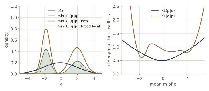
Because KL is not symmetric, “fit \(q\) to \(p\) by minimizing KL” means two different things, and the difference matters whenever the model family cannot represent \(p\) exactly. We fit a single Gaussian \(q(x) = \mathcal{N}(x \mid m, s^2)\) to a density \(p\) with two separated modes.
- Forward KL, \(\mathrm{KL}(p \Vert q)\), averages \(-\ln q\) under \(p\). Wherever \(p\) has mass, \(q\) must not be small, or \(-\ln q\) explodes; so \(q\) spreads to cover both modes. For a Gaussian \(q\), setting the derivatives of \(-\int p \ln q\, dx\) with respect to \(m\) and \(s^2\) to zero gives \(m = \mathbb{E}_p[x]\) and \(s^2 = \operatorname{var}_p[x]\): the best Gaussian matches the mean and variance of \(p\) (moment matching). This is the direction maximum likelihood uses.
- Reverse KL, \(\mathrm{KL}(q \Vert p)\), averages \(\ln(q/p)\) under \(q\). Now \(q\) is punished for putting mass where \(p\) is small, and not at all for ignoring regions where \(p\) is large. So \(q\) tends to lock onto one mode. This is the direction used by variational inference, which we meet with the variational autoencoder in module 19.
We compute the forward fit from the moments. For the reverse fit we evaluate \(\mathrm{KL}(q \Vert p)\) on a grid of \((m, s)\) values and list every grid point that is lower than all its neighbors, that is, every local minimum. All integrals are done numerically.
xk = np.linspace(-8, 8, 3201)
p_bi = 0.55 * gauss_pdf(xk, -1.8, 0.5 ** 2) + 0.45 * gauss_pdf(xk, 2.0, 0.8 ** 2)
ln_p = np.log(p_bi)

def kl_forward(m, s):                                # KL(p || q), q = N(m, s^2)
    return np.trapezoid(p_bi * (ln_p - np.log(gauss_pdf(xk, m, s ** 2))), xk)

def kl_reverse(m, s):                                # KL(q || p)
    q = gauss_pdf(xk, m, s ** 2)
    return np.trapezoid(q * (np.log(q + 1e-300) - ln_p), xk)

m_fwd = np.trapezoid(xk * p_bi, xk)                  # moment matching
s_fwd = np.sqrt(np.trapezoid((xk - m_fwd) ** 2 * p_bi, xk))
print(f"forward KL fit:        m = {m_fwd:.3f}, s = {s_fwd:.3f}   "
      f"KL(p||q) = {kl_forward(m_fwd, s_fwd):.4f}   KL(q||p) = {kl_reverse(m_fwd, s_fwd):.4f}")

ms, ss = np.linspace(-3.5, 3.5, 141), np.linspace(0.2, 3.0, 57)
R = np.array([[kl_reverse(m, s) for s in ss] for m in ms])      # reverse KL on the grid
inner = R[1:-1, 1:-1]
is_min = np.ones(inner.shape, dtype=bool)            # below all eight grid neighbours
for di in (-1, 0, 1):
    for dj in (-1, 0, 1):
        if di or dj:
            is_min &= inner < R[1 + di:R.shape[0] - 1 + di, 1 + dj:R.shape[1] - 1 + dj]
for i, j in zip(*np.nonzero(is_min)):
    m, s = ms[i + 1], ss[j + 1]
    print(f"reverse KL local min:  m = {m:.3f}, s = {s:.3f}   "
          f"KL(q||p) = {R[i + 1, j + 1]:.4f}   KL(p||q) = {kl_forward(m, s):.4f}")
forward KL fit:        m = -0.090, s = 2.000   KL(p||q) = 0.4915   KL(q||p) = 1.1079
reverse KL local min:  m = -1.800, s = 0.500   KL(q||p) = 0.5943   KL(p||q) = 12.4523
reverse KL local min:  m = 0.700, s = 1.700   KL(q||p) = 0.8232   KL(p||q) = 0.6290
reverse KL local min:  m = 1.950, s = 0.850   KL(q||p) = 0.7905   KL(p||q) = 4.7837
The forward fit sits between the modes with a large spread, putting its peak where \(p\) has almost no mass. Reverse KL has three local minima. Two are narrow Gaussians, one on each mode, that ignore the other mode entirely; the one on the heavier left mode is the global minimum. The third is a broad Gaussian between the modes with a higher divergence. Which one an optimizer finds depends on where it starts. Neither answer is wrong; they answer different questions (figure 5).
Conditional entropy
For two variables with joint distribution \(p(\mathbf{x}, \mathbf{y})\), once \(\mathbf{x}\) is known the extra information needed to specify \(\mathbf{y}\) is \(-\ln p(\mathbf{y} \mid \mathbf{x})\). Its average is the conditional entropy
\[\mathrm{H}[\mathbf{y} \mid \mathbf{x}] = -\iint p(\mathbf{y}, \mathbf{x}) \ln p(\mathbf{y} \mid \mathbf{x})\, d\mathbf{y}\, d\mathbf{x}.\]Taking the log of the product rule, \(\ln p(\mathbf{x}, \mathbf{y}) = \ln p(\mathbf{y} \mid \mathbf{x}) + \ln p(\mathbf{x})\), and averaging under \(p(\mathbf{x}, \mathbf{y})\) gives the chain rule
\[\mathrm{H}[\mathbf{x}, \mathbf{y}] = \mathrm{H}[\mathbf{y} \mid \mathbf{x}] + \mathrm{H}[\mathbf{x}].\]Describing both variables costs the information for \(\mathbf{x}\) plus the extra for \(\mathbf{y}\) given \(\mathbf{x}\).
Mutual information
If \(\mathbf{x}\) and \(\mathbf{y}\) are independent, \(p(\mathbf{x}, \mathbf{y}) = p(\mathbf{x})p(\mathbf{y})\). The KL divergence between the joint and the product of the marginals therefore measures how far they are from independent. It is the mutual information
\[\mathrm{I}[\mathbf{x}, \mathbf{y}] \equiv \mathrm{KL}\bigl(p(\mathbf{x}, \mathbf{y}) \Vert p(\mathbf{x})p(\mathbf{y})\bigr) = -\iint p(\mathbf{x}, \mathbf{y}) \ln \frac{p(\mathbf{x})\, p(\mathbf{y})}{p(\mathbf{x}, \mathbf{y})}\, d\mathbf{x}\, d\mathbf{y}.\]By the properties of KL it is non-negative, and zero exactly when the variables are independent. Writing \(p(\mathbf{x}, \mathbf{y}) = p(\mathbf{x} \mid \mathbf{y})p(\mathbf{y})\) inside the log gives
\[\mathrm{I}[\mathbf{x}, \mathbf{y}] = \mathrm{H}[\mathbf{x}] - \mathrm{H}[\mathbf{x} \mid \mathbf{y}] = \mathrm{H}[\mathbf{y}] - \mathrm{H}[\mathbf{y} \mid \mathbf{x}],\]the reduction in uncertainty about one variable from learning the other. In Bayesian terms, with \(p(\mathbf{x})\) as a prior and \(p(\mathbf{x} \mid \mathbf{y})\) as the posterior after observing \(\mathbf{y}\), it is how much, on average, the observation shrinks our uncertainty.
The screening test makes this concrete. How many nats does one test result tell us, on average, about the condition? We also try the test with a tenfold lower false-positive rate.
def info_quantities(prior, sens, fpr):
    joint = np.array([[1 - fpr, fpr], [1 - sens, sens]]) * np.array([[1 - prior], [prior]])
    pC, pT = joint.sum(axis=1), joint.sum(axis=0)
    H_C, H_T, H_CT = entropy(pC), entropy(pT), entropy(joint.ravel())
    H_C_given_T = -np.sum(joint * np.log(joint / pT))           # p(C | T) = p(C, T) / p(T)
    I_kl = np.sum(joint * np.log(joint / np.outer(pC, pT)))     # KL(joint || product)
    return H_C, H_T, H_CT, H_C_given_T, I_kl

H_C, H_T, H_CT, H_C_T, I_kl = info_quantities(prior, sens, fpr)
print(f"H[C] {H_C:.5f}   H[C|T] {H_C_T:.5f}   I = H[C] - H[C|T] = {H_C - H_C_T:.5f}   "
      f"I as a KL: {I_kl:.5f} nats")
print(f"chain rule: H[C,T] {H_CT:.5f} = H[C|T] + H[T] = {H_C_T + H_T:.5f}")
_, _, _, _, I_better = info_quantities(prior, sens, fpr / 10)
print(f"false-positive rate 0.2%: I = {I_better:.5f} nats "
      f"({I_better / H_C:.0%} of H[C], versus {I_kl / H_C:.0%})")
H[C] 0.02608   H[C|T] 0.01310   I = H[C] - H[C|T] = 0.01297   I as a KL: 0.01297 nats
chain rule: H[C,T] 0.12484 = H[C|T] + H[T] = 0.12484
false-positive rate 0.2%: I = 0.01951 nats (75% of H[C], versus 50%)
A single result removes about half of our (already small) uncertainty about the condition; with a tenfold lower false-positive rate it removes three quarters. Mutual information is a single number that rates a test, or more generally how much a feature or a learned representation tells us about a quantity of interest.
Bayesian probabilities
So far we have mostly read probabilities as frequencies of repeatable events: the fraction of people who test positive. Probabilities can also express uncertainty about things that are not repeatable at all. Whether a particular coin in your pocket is biased, or what the right weights of a network are, is not the outcome of a random experiment; it is simply unknown. Using probability for such degrees of belief is the Bayesian interpretation, and the frequency reading is the frequentist or classical one. The Bayesian use is not an arbitrary choice: Cox (1946) showed that any numerical measure of belief obeying a few common-sense consistency requirements must follow the sum and product rules, which makes such beliefs probabilities.
The Bayesian reading brings prior knowledge in naturally. If a coin that looks ordinary lands heads four times out of four, maximum likelihood estimates the probability of heads as 1 and predicts heads forever. A Bayesian with any sensible prior, one that puts most belief near 0.5, reaches a much milder conclusion. Module 03 works this out with the beta distribution.
Model parameters
Apply this to the parameters \(\mathbf{w}\) of a model trained on a data set \(\mathcal{D}\). Before seeing the data, we describe what we believe about \(\mathbf{w}\) with a prior \(p(\mathbf{w})\). The data enter through \(p(\mathcal{D} \mid \mathbf{w})\), and Bayes’ theorem gives the posterior:
\[p(\mathbf{w} \mid \mathcal{D}) = \frac{p(\mathcal{D} \mid \mathbf{w})\, p(\mathbf{w})}{p(\mathcal{D})}, \qquad p(\mathcal{D}) = \int p(\mathcal{D} \mid \mathbf{w})\, p(\mathbf{w})\, d\mathbf{w}.\]Definition. Viewed as a function of \(\mathbf{w}\) with the data fixed, \(p(\mathcal{D} \mid \mathbf{w})\) is the likelihood function. It is not a probability distribution over \(\mathbf{w}\), and its integral over \(\mathbf{w}\) need not be one. In words: posterior ∝ likelihood × prior, and the denominator \(p(\mathcal{D})\) is the normalizing constant.
Maximum likelihood uses only the likelihood and returns one \(\mathbf{w}_{\mathrm{ML}}\); its negative log is the error function. The frequentist view treats \(\mathbf{w}\) as fixed and describes uncertainty by how the estimate would vary over hypothetical repeated data sets. The Bayesian view conditions on the one data set we actually have and describes uncertainty by the spread of the posterior.
The smallest example that shows the posterior at work has one parameter. Let \(t = w x + \epsilon\) with Gaussian noise of known standard deviation \(\sigma = 0.5\), and a prior \(w \sim \mathcal{N}(0, 1)\). We compute the posterior on a grid of \(w\) values by multiplying the likelihood by the prior and normalizing, and compare with the exact answer: because everything is Gaussian, the posterior is Gaussian with precision \(1/s_0^2 + \sum_n x_n^2/\sigma^2\) and mean \(\left(\sum_n x_n t_n/\sigma^2\right)\) divided by that precision (module 04 derives this for general linear models).
w_true, sig_t, s0 = 0.8, 0.5, 1.0
x_all = rng.uniform(-2, 2, 50)
t_all = w_true * x_all + rng.normal(0, sig_t, 50)
w_grid = np.linspace(-6, 6, 12_001)

for N in [1, 5, 50]:
    x_n, t_n = x_all[:N], t_all[:N]
    log_post = (-0.5 * ((t_n[None, :] - w_grid[:, None] * x_n[None, :]) ** 2).sum(axis=1)
                / sig_t ** 2 - 0.5 * w_grid ** 2 / s0 ** 2)        # ln likelihood + ln prior
    post = np.exp(log_post - log_post.max())
    post /= np.trapezoid(post, w_grid)                             # divide by p(D)
    m_grid = np.trapezoid(w_grid * post, w_grid)
    sd_grid = np.sqrt(np.trapezoid((w_grid - m_grid) ** 2 * post, w_grid))
    prec = 1 / s0 ** 2 + np.sum(x_n ** 2) / sig_t ** 2
    m_exact = np.sum(x_n * t_n) / sig_t ** 2 / prec
    print(f"N = {N:2d}: posterior mean {m_grid:.4f} (exact {m_exact:.4f})   "
          f"s.d. {sd_grid:.4f} (exact {1 / np.sqrt(prec):.4f})")
N =  1: posterior mean -0.1710 (exact -0.1710)   s.d. 0.9711 (exact 0.9711)
N =  5: posterior mean 0.2889 (exact 0.2889)   s.d. 0.2149 (exact 0.2149)
N = 50: posterior mean 0.7735 (exact 0.7735)   s.d. 0.0599 (exact 0.0599)
As data accumulate, the posterior concentrates around the true value 0.8 and its standard deviation shrinks roughly like \(1/\sqrt{N}\): epistemic uncertainty falling as we observe more.
Regularization as MAP estimation
The posterior also explains regularization. Instead of maximizing the likelihood, we can pick the \(\mathbf{w}\) that maximizes the posterior, the maximum a posteriori or MAP estimate. Taking negative logs of Bayes’ theorem,
\[-\ln p(\mathbf{w} \mid \mathcal{D}) = -\ln p(\mathcal{D} \mid \mathbf{w}) - \ln p(\mathbf{w}) + \ln p(\mathcal{D}).\]The first term is the usual error function, the last does not depend on \(\mathbf{w}\), and the middle term is new: a function of \(\mathbf{w}\) added to the error, which is exactly what a regularizer is. For a prior that makes each of the \(M\) weights an independent zero-mean Gaussian with variance \(s^2\),
\[p(\mathbf{w} \mid s) = \prod_{i=1}^{M} \mathcal{N}(w_i \mid 0, s^2), \qquad -\ln p(\mathbf{w} \mid s) = \frac{1}{2s^2} \sum_{i=1}^{M} w_i^2 + \text{const}.\]With the Gaussian-noise likelihood of the regression section, MAP estimation minimizes
\[\frac{1}{2\sigma^2} \sum_{n=1}^{N} \bigl\{ y(x_n, \mathbf{w}) - t_n \bigr\}^2 + \frac{1}{2s^2}\, \mathbf{w}^{\mathrm{T}}\mathbf{w},\]which after multiplying by \(\sigma^2\) is the regularized sum-of-squares error of module 01 with coefficient \(\lambda = \sigma^2/s^2\). A broad prior (large \(s\)) means weak regularization; a narrow one means strong regularization.
In gradient descent this penalty has a memorable form. The gradient of \(\frac{\lambda}{2}\mathbf{w}^{\mathrm{T}}\mathbf{w}\) is \(\lambda\mathbf{w}\), so each step with learning rate \(\eta\) becomes
\[\mathbf{w} \leftarrow (1 - \eta\lambda)\, \mathbf{w} - \eta \nabla E(\mathbf{w}),\]which shrinks every weight by a constant factor before the usual update. This is weight decay, one of the most common regularizers in deep learning (module 09). We run it on the cubic regression problem from earlier and compare with the closed-form MAP solution \((\boldsymbol{\Phi}^{\mathrm{T}}\boldsymbol{\Phi} + \lambda\mathbf{I})\mathbf{w} = \boldsymbol{\Phi}^{\mathrm{T}}\mathsf{t}\).
lam_wd = sigma_noise ** 2 / 0.5 ** 2                # prior s.d. 0.5 on each weight
w_map = np.linalg.solve(Phi.T @ Phi + lam_wd * np.eye(4), Phi.T @ t_tr)

w_gd = np.zeros(4)
eta = 0.01
for step in range(1, 20_001):
    grad_E = Phi.T @ (Phi @ w_gd - t_tr)            # gradient of the sum-of-squares error
    w_gd = (1 - eta * lam_wd) * w_gd - eta * grad_E # weight decay step
    if step in (10, 100, 1000, 20_000):
        print(f"step {step:6d}: distance to the MAP solution {np.linalg.norm(w_gd - w_map):.2e}")
print("w_MAP:", w_map)
print("w_ML: ", w_ml)
step     10: distance to the MAP solution 1.83e+00
step    100: distance to the MAP solution 4.62e-01
step   1000: distance to the MAP solution 5.15e-07
step  20000: distance to the MAP solution 5.00e-15
w_MAP: [ 0.0196  1.8987 -0.1208 -1.1509]
w_ML:  [ 0.0216  1.9914 -0.1193 -1.2481]
Weight decay converges to the MAP solution, and the prior pulls the larger coefficients toward zero compared with maximum likelihood.
Watch out. A MAP estimate is the mode of a density, so, as we saw with \(\tanh\), it depends on how the parameters are written. Put the same prior on \(\ln s\) instead of \(s\) and the most probable value changes. The posterior itself transforms consistently; only its single “best point” does not. This is one reason Bayesian methods prefer to keep the whole posterior.
Bayesian machine learning
MAP is still a point estimate: one \(\mathbf{w}\), with the posterior’s spread thrown away. A fully Bayesian prediction for a new input \(x\) averages the predictions of all weight vectors, weighted by the posterior. By the sum and product rules,
\[p(t \mid x, \mathcal{D}) = \int p(t \mid x, \mathbf{w})\, p(\mathbf{w} \mid \mathcal{D})\, d\mathbf{w}.\]This integral over parameters is what distinguishes Bayesian methods. It gives predictions whose spread includes our uncertainty about \(\mathbf{w}\) (epistemic) on top of the noise (aleatoric), and it does not overfit in the way maximum likelihood does, because no single over-tuned \(\mathbf{w}\) is chosen. The same principle applied one level up compares models of different complexity, averaging over each model’s parameters and weighting models by their posterior probabilities; that tends to favor models of intermediate complexity.
For the one-parameter model the integral has a closed form: the predictive distribution is Gaussian with mean \(m_N x\) and variance \(\sigma^2 + x^2 s_N^2\), where \(m_N\) and \(s_N^2\) are the posterior mean and variance. We check it by Monte Carlo, averaging \(p(t \mid x, w)\) over samples of \(w\) from the posterior, and compare it with the plug-in prediction that uses only the MAP value.
N = 5
x_n, t_n = x_all[:N], t_all[:N]
prec = 1 / s0 ** 2 + np.sum(x_n ** 2) / sig_t ** 2
m_N, s2_N = np.sum(x_n * t_n) / sig_t ** 2 / prec, 1 / prec    # Gaussian posterior (= MAP at m_N)
w_post = rng.normal(m_N, np.sqrt(s2_N), 200_000)               # samples from p(w | D)

t_eval = 1.0
for x_new in [0.5, 2.0, 6.0]:
    mc = gauss_pdf(t_eval, w_post * x_new, sig_t ** 2).mean()  # average of p(t | x, w)
    exact = gauss_pdf(t_eval, m_N * x_new, sig_t ** 2 + x_new ** 2 * s2_N)
    print(f"x = {x_new}: predictive s.d. {np.sqrt(sig_t ** 2 + x_new ** 2 * s2_N):.3f} "
          f"(plug-in {sig_t:.3f})   p(t=1 | x, D): Monte Carlo {mc:.4f}, exact {exact:.4f}")
x = 0.5: predictive s.d. 0.511 (plug-in 0.500)   p(t=1 | x, D): Monte Carlo 0.1923, exact 0.1925
x = 2.0: predictive s.d. 0.659 (plug-in 0.500)   p(t=1 | x, D): Monte Carlo 0.4922, exact 0.4930
x = 6.0: predictive s.d. 1.383 (plug-in 0.500)   p(t=1 | x, D): Monte Carlo 0.2508, exact 0.2506
Near the data the Bayesian and plug-in predictions nearly agree. Far from them, at \(x = 6\), the Bayesian predictive spread is more than twice the noise level, because a small uncertainty in the slope becomes a large uncertainty in the prediction; the plug-in prediction is just as confident there as anywhere.
Why deep learning mostly uses point estimates. The integral over \(\mathbf{w}\) is the obstacle. For our one weight we could use a grid; for a network with millions or billions of weights, neither grids nor exact formulas exist, and even rough approximations to the posterior are expensive. In practice, given a fixed compute budget and plenty of data, it is usually better to train a larger network by maximum likelihood with regularization than to treat a much smaller network in a fully Bayesian way. Most of this course therefore trains point estimates (maximum likelihood or MAP), while borrowing Bayesian ideas where they are cheap: priors as regularizers, averaging over several trained models, and the variational methods of modules 16 and 19. The Intro to ML notes show approximate Bayesian treatments of networks with the Laplace approximation (Intro to ML, module 05).
In practice. When a network’s confidence matters (medical screening is the obvious case), remember that a single trained network reports only aleatoric uncertainty, through its output distribution. Epistemic uncertainty, the kind that grows far from the training data as in the \(x = 6\) example, needs something extra: an ensemble of networks trained from different initializations, or an approximate posterior.
Summary
| Idea | What it says | Key equation or property |
|---|---|---|
| Sum and product rules | marginals sum joints; joints factor into conditional × marginal | \(p(X) = \sum_Y p(X, Y)\), \(p(X, Y) = p(Y \mid X)p(X)\) |
| Bayes’ theorem | reverses a conditional; posterior ∝ likelihood × prior | \(p(Y \mid X) = p(X \mid Y)p(Y)/p(X)\) |
| Expectations | averages under a distribution; sample averages estimate them | mini-batch gradients are unbiased, s.d. \(\propto 1/\sqrt{B}\) |
| Gaussian maximum likelihood | sample mean and sample variance | \(\mathbb{E}[\sigma^2_{\mathrm{ML}}] = \frac{N-1}{N}\sigma^2\) |
| Regression as maximum likelihood | Gaussian noise turns the negative log-likelihood into squared error | \(-\ln p = E(\mathbf{w})/\sigma^2 + \text{const}\) |
| Change of variables | densities pick up the Jacobian; modes move | \(p_{\mathbf{y}}(\mathbf{y}) = p_{\mathbf{x}}(\mathbf{g}(\mathbf{y}))\,\lvert\det\mathbf{J}\rvert\) |
| Entropy | average information; maximal for uniform (discrete) or Gaussian (fixed variance) | \(\mathrm{H} = \frac12\{1 + \ln(2\pi\sigma^2)\}\) for \(\mathcal{N}(\mu, \sigma^2)\) |
| KL divergence and cross-entropy | extra code length from using \(q\) for \(p\); ML and the classification loss minimize it | \(\mathrm{H}[p, q] = \mathrm{H}[p] + \mathrm{KL}(p \Vert q)\), \(\mathrm{KL} \ge 0\) |
| Mutual information | how much one variable tells about another | \(\mathrm{I}[x, y] = \mathrm{H}[x] - \mathrm{H}[x \mid y]\) |
| MAP and weight decay | Gaussian prior = quadratic penalty | \(\lambda = \sigma^2/s^2\), \(\mathbf{w} \leftarrow (1 - \eta\lambda)\mathbf{w} - \eta\nabla E\) |
| Bayesian prediction | average predictions over the posterior | \(p(t \mid x, \mathcal{D}) = \int p(t \mid x, \mathbf{w})\,p(\mathbf{w} \mid \mathcal{D})\,d\mathbf{w}\) |
Ideas to carry forward:
- A loss is a negative log-likelihood. Choose a distribution for the target given the network output and the loss follows: squared error for Gaussian targets, cross-entropy for class labels. Minimizing it minimizes a KL divergence from the data to the model.
- Densities transform with a Jacobian. Invertible maps with cheap Jacobian determinants turn a simple density into a flexible one; this is the core of normalizing flows (module 18), and the reason “most probable value” depends on parameterization.
- Forward and reverse KL behave differently. Forward KL (maximum likelihood) covers all of the data’s modes; reverse KL (variational inference) tends to lock onto one.
- Point estimates are a practical choice, not the whole story. Priors become regularizers, but the uncertainty in the weights is discarded unless we do something extra to keep it.
Exercises
- After a positive first test, a patient takes the same test again and it comes back negative. Assuming conditional independence of the two results given \(C\), compute \(p(C = 1 \mid T_1 = 1, T_2 = 0)\) with our test’s numbers, and check it with the simulated population by adding a second, independent test result. Then explain in a sentence why conditional independence might fail for two runs of the same blood test on the same sample.
- A mini-batch of size \(B\) is drawn without replacement from \(N\) examples. Show that the mini-batch average of per-example gradients is unbiased and that the variance of each component is \(\frac{\sigma_g^2}{B} \cdot \frac{N - B}{N - 1}\), where \(\sigma_g^2\) is the variance of that component over the data set. Check the factor against the \(B = 1000\) line of the mini-batch experiment.
- For i.i.d. Gaussian data, \(\sigma^2_{\mathrm{ML}}\) is biased and \(\widetilde{\sigma}^2 = \frac{N}{N-1}\sigma^2_{\mathrm{ML}}\) is not. Using the simulation code, compare their mean squared errors \(\mathbb{E}[(\text{estimate} - \sigma^2)^2]\) for \(N = 3, 5, 20\). Which is closer to the truth on average? Find by simulation the multiplier \(c\) for which \(c \sum_n (x_n - \mu_{\mathrm{ML}})^2\) has the smallest mean squared error, and compare it with \(1/(N+1)\).
- Let the noise level depend on the input: \(p(t \mid x) = \mathcal{N}\bigl(t \mid y(x, \mathbf{w}), \sigma(x)^2\bigr)\) with \(\ln \sigma(x) = v_0 + v_1 x\). Write the negative log-likelihood, derive its gradients with respect to \(\mathbf{w}\), \(v_0\), and \(v_1\), and fit a cubic \(y\) and the two \(v\)’s by gradient descent to data whose noise standard deviation grows from 0.05 at \(x = -1.2\) to 0.4 at \(x = 1.2\). Why does parameterizing \(\ln\sigma\) rather than \(\sigma\) help?
- Let \(x \sim \mathcal{N}(0, 1)\) and \(y = \ln(1 + e^{x})\) (the softplus). Derive \(p_y(y)\) for \(y > 0\), find its mode numerically, and compare with the image of the mode of \(x\). Check \(p_y\) against a histogram of transformed samples.
- Compose two coupling layers: the first transforms \(x_2\) given \(x_1\) as in the notes, the second transforms the new first coordinate given the new second coordinate with its own functions \(s'\) and \(b'\). Show that the log-determinant of the composition is the sum of the two layers’ log-determinants, implement the composed density, and verify that it integrates to one and matches a histogram of samples.
- A classifier’s softmax with temperature \(\tau\) is \(y_k = \exp(a_k/\tau)/\sum_j \exp(a_j/\tau)\). Show that the entropy of \(\mathbf{y}\) tends to 0 as \(\tau \to 0\) (when the largest logit is unique) and to \(\ln K\) as \(\tau \to \infty\). Plot the entropy against \(\tau\) for the logits \((2, 1, 0.5, -1)\).
- Derive the KL divergence between two univariate Gaussians \(\mathcal{N}(\mu_1, \sigma_1^2)\) and \(\mathcal{N}(\mu_2, \sigma_2^2)\) and check it against numerical integration. Then prove the moment-matching result used for the forward KL fit: among Gaussians \(q\), \(\mathrm{KL}(p \Vert q)\) is minimized by the mean and variance of \(p\).
- With label smoothing, the target for class \(c\) is \(t_k = (1 - \epsilon)\,[k = c] + \epsilon/K\). Show that the cross-entropy loss becomes \((1 - \epsilon)(-\ln y_c) + \epsilon \cdot \frac{1}{K}\sum_k (-\ln y_k)\), and that its minimum over \(\mathbf{y}\) is at \(\mathbf{y} = \mathbf{t}\). What is the gap \(a_c - a_k\) between logits at that minimum? Why does this stop logits from growing without bound?
- Replace the Gaussian prior on the single weight \(w\) by a Laplace prior \(p(w) \propto \exp(-\lvert w \rvert/b)\). Show that the MAP estimate minimizes a squared error plus an absolute-value penalty, derive the closed form (a “soft threshold” of the least-squares estimate), and check it against the grid posterior. For which data does the MAP estimate come out exactly zero?
- For the one-parameter Bayesian model with \(N = 3\) data points, generate 5,000 test pairs with \(x\) uniform on \((-6, 6)\). What fraction of targets falls inside the central 95% interval of the Bayesian predictive distribution, and of the MAP plug-in distribution? Where do the misses of the plug-in model concentrate?
- In your own words: what is the difference between aleatoric and epistemic uncertainty, which of the two does a network trained by maximum likelihood with a Gaussian or softmax output represent, and what would you have to add to represent the other?
Going further
- C. M. Bishop and H. Bishop, Deep Learning: Foundations and Concepts, chapter 2 — the source for this module. Exercise 2.1 revisits the screening example with a lower prevalence, 2.2 is a pleasant puzzle about non-transitive dice, 2.12–2.18 cover the Gaussian’s moments and the bias of maximum likelihood, 2.19–2.20 are about transformations of densities, 2.21–2.38 cover entropy, KL divergence, Jensen’s inequality, and mutual information, and 2.40–2.41 are Bayesian.
- Intro to ML, module 01 covers the same ground from Pattern Recognition and Machine Learning, with more on decision theory and model selection; Intro to ML, module 02 develops the Gaussian, conjugate priors, and Bayesian inference for the Gaussian’s parameters; Intro to ML, module 10 uses reverse KL for variational inference.
- D. J. C. MacKay, Information Theory, Inference, and Learning Algorithms, Cambridge University Press, 2003 (free online) — entropy, coding, and Bayesian inference in one book, with many worked examples.
- T. M. Cover and J. A. Thomas, Elements of Information Theory, 2nd ed., Wiley, 2006 — the standard reference for entropy, KL divergence, and mutual information.
- C. E. Shannon, “A mathematical theory of communication”, Bell System Technical Journal, 1948 — where entropy and the coding theorem come from.
- In this course: module 03 (standard distributions and the multivariate Gaussian), module 05 (cross-entropy for classifiers), and module 18 (normalizing flows, built on the change of variables).
These notes follow the chapters of C. M. Bishop and H. Bishop, Deep Learning: Foundations and Concepts (Springer, 2024), the course text, which the authors make free to read online. The explanations, code, figures, and exercises here are written for this course; the book remains the reference, with the full derivations and many more exercises.