CSE 676 · Module 18 · Week 13
Normalizing Flows
Invertible networks with tractable Jacobians — coupling flows, masked and inverse autoregressive flows, and continuous flows built from neural ordinary differential equations.
Companion reading: Bishop & Bishop, Deep Learning: Foundations and Concepts, chapter 18, “Normalizing Flows”
By the end of this module you can
- Write the exact log likelihood of an invertible network with the change-of-variables formula, and explain why a stack of invertible layers has a log-determinant equal to the sum of the layers’ log-determinants.
- Build an affine coupling layer from tensor operations, derive its triangular Jacobian, and verify its inverse and log-determinant against
torch.autograd.functional.jacobian. - Train a stack of coupling layers by maximum likelihood on two-dimensional data and compare its test log likelihood with a Gaussian and with the true density.
- Construct MADE masks, verify that they make the Jacobian triangular, and explain why a masked autoregressive flow evaluates densities in one pass but samples in D passes, while an inverse autoregressive flow does the opposite.
- Write a fourth-order Runge–Kutta integrator, measure its order of accuracy, and describe a neural ODE as the limit of a residual network.
- Derive the adjoint equations for a neural ODE, implement them, and compare the gradients and memory cost with backpropagation through the solver.
- Derive the instantaneous change of variables, train a continuous normalizing flow with an exact trace, and check that its density integrates to one.
- Show that Hutchinson’s trace estimator is unbiased, compute its variance for Gaussian and Rademacher probes, and confirm both numerically.
Contents
- Invertible networks and exact likelihoods
- Coupling flows
- Autoregressive flows
- Continuous flows
- Summary
- Exercises
- Going further
A generative model that maps a simple latent variable \(\mathbf{z}\) through a neural network to a data point \(\mathbf{x}\) is easy to sample from, but its likelihood is usually out of reach. The GANs of module 17 gave up on the likelihood and trained with a second, adversarial network instead. This module takes another road: restrict the network so that it can be inverted, and use the change-of-variables formula from module 02 to write down the likelihood exactly. Models of this kind are called normalizing flows.
Invertibility alone is not enough. The change-of-variables formula contains the determinant of a \(D \times D\) Jacobian matrix, which costs \(O(D^3)\) operations in general, far too much to compute for every data point at every training step. So each family of flows is a design for layers that are invertible and have a Jacobian whose determinant is cheap. We build three: coupling flows, where half of the variables pass through unchanged and control a simple transformation of the other half; autoregressive flows, where each variable is transformed conditionally on the ones before it; and continuous flows, where the transformation is the solution of a neural ordinary differential equation and the determinant is replaced by a trace.
Everything is written from tensor operations in PyTorch and checked numerically: inverses by round trips, log-determinants against Jacobians computed by automatic differentiation, adjoint gradients against backpropagation through the solver, and a trace estimator against the exact trace. All the models are trained on a two-dimensional “two moons” data set that we generate ourselves, for which we can compute the true density and so know the best log likelihood any model could reach. The last part connects to residual networks (module 09) and points ahead to the diffusion models of module 20.
import math
import time
import numpy as np
import torch
import torch.nn as nn
import torch.nn.functional as F

np.set_printoptions(precision=4, suppress=True)
rng = np.random.default_rng(18)
torch.manual_seed(18)
Invertible networks and exact likelihoods
The change of variables, recalled
Choose a simple base distribution \(p_{\mathbf{z}}(\mathbf{z})\) over a latent vector \(\mathbf{z}\), in this module always the standard Gaussian \(\mathcal{N}(\mathbf{z} \mid \mathbf{0}, \mathbf{I})\), and a network \(\mathbf{x} = \mathbf{f}(\mathbf{z}, \mathbf{w})\) that maps latent vectors to data vectors. Sampling is easy: draw \(\mathbf{z}\) and push it through \(\mathbf{f}\). For the likelihood we need to go the other way. Suppose \(\mathbf{f}\) is bijective (one-to-one and onto) for every value of the weights, and write its inverse as \(\mathbf{z} = \mathbf{g}(\mathbf{x}, \mathbf{w})\), so that \(\mathbf{g}(\mathbf{f}(\mathbf{z}, \mathbf{w}), \mathbf{w}) = \mathbf{z}\). Module 02 showed that probability is conserved under such a map, which gives
\[p_{\mathbf{x}}(\mathbf{x} \mid \mathbf{w}) = p_{\mathbf{z}}\bigl(\mathbf{g}(\mathbf{x}, \mathbf{w})\bigr)\, \bigl\lvert \det \mathbf{J}(\mathbf{x}) \bigr\rvert, \qquad J_{ij}(\mathbf{x}) = \frac{\partial g_i(\mathbf{x}, \mathbf{w})}{\partial x_j}.\](The same formula, read in the sampling direction, is the transformation method for generating random numbers in Intro to ML, module 11.) The determinant is the factor by which \(\mathbf{g}\) changes volume near \(\mathbf{x}\): where the network squeezes a large region of latent space into a small region of data space, the data density is high. Even though the map is deterministic, we keep calling \(\mathbf{z}\) the latent variable.
It is often easier to work with the Jacobian of the forward map, \(K_{ij} = \partial f_i / \partial z_j\). Differentiating the identity \(\mathbf{f}(\mathbf{g}(\mathbf{x})) = \mathbf{x}\) with the chain rule gives \(\mathbf{K}\mathbf{J} = \mathbf{I}\), with \(\mathbf{K}\) evaluated at \(\mathbf{z} = \mathbf{g}(\mathbf{x})\). Taking determinants, \(\det \mathbf{J} = 1 / \det \mathbf{K}\), so
\[\ln p_{\mathbf{x}}(\mathbf{x} \mid \mathbf{w}) = \ln p_{\mathbf{z}}(\mathbf{z}) + \ln \bigl\lvert \det \mathbf{J}(\mathbf{x}) \bigr\rvert = \ln p_{\mathbf{z}}(\mathbf{z}) - \ln \bigl\lvert \det \mathbf{K}(\mathbf{z}) \bigr\rvert, \qquad \mathbf{z} = \mathbf{g}(\mathbf{x}, \mathbf{w}).\]For a training set \(\mathcal{D} = \{\mathbf{x}_1, \dots, \mathbf{x}_N\}\) of independent points the log likelihood is the sum of this over \(n\), and we maximize it by stochastic gradient descent, with automatic differentiation providing the gradients. Nothing is approximated: this is the exact likelihood of the model.
One consequence is built into the setup: an invertible map needs \(\mathbf{z}\) and \(\mathbf{x}\) to have the same dimension \(D\). A flow cannot compress, unlike the latent-variable models of module 16 and the autoencoders of module 19, and for images it carries a latent vector as large as the image.
Composing invertible layers
We make \(\mathbf{f}\) flexible the usual way, by stacking layers, and keep it invertible by making each layer invertible. If \(\mathbf{x} = \mathbf{f}_L(\cdots \mathbf{f}_2(\mathbf{f}_1(\mathbf{z})))\), the inverse applies the layer inverses in the opposite order, \(\mathbf{z} = \mathbf{g}_1(\mathbf{g}_2(\cdots \mathbf{g}_L(\mathbf{x})))\). By the chain rule the Jacobian of the composition is the product of the layer Jacobians, each evaluated at the intermediate point where the layer acts, and determinants multiply, \(\det(\mathbf{A}\mathbf{B}) = \det\mathbf{A}\,\det\mathbf{B}\). Taking logarithms,
\[\ln \bigl\lvert \det \mathbf{J}(\mathbf{x}) \bigr\rvert = \sum_{l=1}^{L} \ln \bigl\lvert \det \mathbf{J}_l \bigr\rvert ,\]where \(\mathbf{J}_l\) is the Jacobian of \(\mathbf{g}_l\) at its own input. A flow is therefore a sequence of layers, each of which can run forward, run backward, and report its own log-determinant; the model just adds them up. The name comes from this picture: a simple density is transported through a sequence of maps, like a fluid, and the inverse direction turns (“normalizes”) the complicated data density into a standard normal one.
Which layers qualify? A layer must be invertible, its inverse must be cheap to compute (for the likelihood), and its log-determinant must be cheap. The rest of the module is about three answers to that design problem.
A running example: two moons
Our data are two interleaved half-circles blurred by Gaussian noise. We generate them ourselves, so we also know the exact density: a point is produced by choosing a moon with probability \(\tfrac12\), an angle \(\theta\) uniformly in \([0, \pi]\), and adding isotropic noise of standard deviation \(\sigma = 0.12\) to the point \(\mathbf{c}_k(\theta)\) on the chosen arc. Hence
\[p(\mathbf{x}) = \frac{1}{2} \sum_{k=1}^{2} \frac{1}{\pi} \int_0^{\pi} \mathcal{N}\bigl(\mathbf{x} \mid \mathbf{c}_k(\theta), \sigma^2 \mathbf{I}\bigr)\, d\theta ,\]and the integral over the angle is one-dimensional, so the trapezoid rule on a fine grid evaluates it to high accuracy.
SIGMA, SCALE = 0.12, 1.6
SHIFT = torch.tensor([0.5, 0.25])

def moon_centers(theta, which):
    """Points c_k(theta) on the upper (which = 0) or lower (which = 1) arc."""
    c, s = torch.cos(theta), torch.sin(theta)
    upper = torch.stack([c, s], dim=1)
    lower = torch.stack([1 - c, 0.5 - s], dim=1)
    arc = torch.where(which[:, None] == 0, upper, lower)
    return SCALE * (arc - SHIFT)

def make_moons(N, gen):
    which = torch.randint(0, 2, (N,), generator=gen)
    theta = math.pi * torch.rand(N, generator=gen)
    return moon_centers(theta, which) + SIGMA * torch.randn(N, 2, generator=gen), which

def true_log_prob(x, n_theta=721):
    """Exact ln p(x): the integral over the angle by the trapezoid rule, in log space."""
    theta = torch.linspace(0, math.pi, n_theta)
    w = torch.full((n_theta,), 1.0 / (n_theta - 1))
    w[[0, -1]] *= 0.5                                    # trapezoid weights; they sum to 1
    parts = []
    for k in range(2):
        c = moon_centers(theta, torch.full((n_theta,), k))
        d2 = ((x[:, None, :] - c[None]) ** 2).sum(-1)
        log_gauss = -0.5 * d2 / SIGMA**2 - math.log(2 * math.pi * SIGMA**2)
        parts.append(math.log(0.5) + torch.logsumexp(log_gauss + torch.log(w), dim=1))
    return torch.logaddexp(parts[0], parts[1])

gen = torch.Generator().manual_seed(18)
X_train, _ = make_moons(3000, gen)
X_test, moon_test = make_moons(3000, gen)
print("X_train", tuple(X_train.shape), "  mean", X_train.mean(0).numpy(),
      "  std", X_train.std(0).numpy())

gauss = torch.distributions.MultivariateNormal(X_train.mean(0), torch.cov(X_train.T))
print(f"test NLL, true density     {-true_log_prob(X_test).mean().item():.4f} nats")
print(f"test NLL, fitted Gaussian  {-gauss.log_prob(X_test).mean().item():.4f} nats")
X_train (3000, 2)   mean [-0.0226  0.0009]   std [1.3949 0.7967]
test NLL, true density     1.6668 nats
test NLL, fitted Gaussian  2.8370 nats
The negative log likelihood (NLL) per test point is our score throughout. For any model \(q\), the expected NLL under the data distribution \(p\) is \(\mathbb{E}_p[-\ln q] = \mathrm{H}[p] + \mathrm{KL}(p \Vert q)\), the entropy of \(p\) plus a nonnegative divergence. The true-density line is a Monte Carlo estimate of this entropy, the floor no model can beat on average; a fitted Gaussian sits more than a nat above it. A flow should close most of that gap.
Coupling flows
Why linear layers are not enough
The simplest invertible layer is linear, \(\mathbf{x} = \mathbf{A}\mathbf{z} + \mathbf{b}\) with \(\mathbf{A}\) invertible. Its inverse and its determinant are easy, but a composition of linear maps is again a linear map, and a linear map of a Gaussian is a Gaussian. However many such layers we stack, the model is the fitted Gaussian above. We need layers that are nonlinear but keep the two properties that made the linear layer attractive.
The affine coupling layer
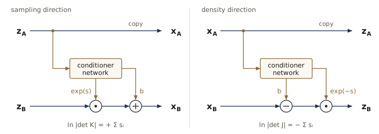
The real NVP layer (for “real-valued non-volume-preserving”; Dinh, Sohl-Dickstein, and Bengio) gets there with a clever split. Divide the latent vector into two blocks, \(\mathbf{z} = (\mathbf{z}_A, \mathbf{z}_B)\), with \(d\) and \(D - d\) components, and split the output the same way. The first block is copied, and the second block goes through an elementwise affine map whose scale and shift are computed from the first block by neural networks:
\[\mathbf{x}_A = \mathbf{z}_A, \qquad \mathbf{x}_B = \exp\bigl(\mathbf{s}(\mathbf{z}_A, \mathbf{w})\bigr) \odot \mathbf{z}_B + \mathbf{b}(\mathbf{z}_A, \mathbf{w}).\]Here \(\odot\) is the elementwise product, the exponential acts elementwise and keeps every scale positive, and \(\mathbf{s}\) (the log-scales) and \(\mathbf{b}\) (the shifts) are outputs of an ordinary network, in practice one network with \(2(D - d)\) outputs.
The inverse needs no inversion of any network. Given \(\mathbf{x}\), the first block is already known, \(\mathbf{z}_A = \mathbf{x}_A\); feeding it to the network reproduces exactly the same \(\mathbf{s}\) and \(\mathbf{b}\) that the forward pass used, and the affine map is undone:
\[\mathbf{z}_A = \mathbf{x}_A, \qquad \mathbf{z}_B = \exp\bigl(-\mathbf{s}(\mathbf{x}_A, \mathbf{w})\bigr) \odot \bigl(\mathbf{x}_B - \mathbf{b}(\mathbf{x}_A, \mathbf{w})\bigr).\]The networks \(\mathbf{s}\) and \(\mathbf{b}\) can be as complicated as we like and need not be invertible themselves; they are only ever evaluated, never inverted.
Its Jacobian is triangular
Order the variables as \((\mathbf{x}_A, \mathbf{x}_B)\) and write the Jacobian of the inverse map in blocks:
\[\mathbf{J} = \frac{\partial (\mathbf{z}_A, \mathbf{z}_B)}{\partial (\mathbf{x}_A, \mathbf{x}_B)} = \begin{pmatrix} \mathbf{I}_d & \mathbf{0} \\[2pt] \dfrac{\partial \mathbf{z}_B}{\partial \mathbf{x}_A} & \operatorname{diag}\bigl(\exp(-\mathbf{s})\bigr) \end{pmatrix}.\]The top row holds the derivatives of \(\mathbf{z}_A = \mathbf{x}_A\): the identity with respect to \(\mathbf{x}_A\) and zero with respect to \(\mathbf{x}_B\). The bottom-right block is diagonal because \(z_{B,i}\) depends on \(x_{B,i}\) only through its own scale and shift. The bottom-left block contains derivatives of the networks \(\mathbf{s}\) and \(\mathbf{b}\), which are messy, but they sit below the diagonal. The matrix is lower triangular, and the determinant of a triangular matrix is the product of its diagonal. The messy block never enters.
Result. For an affine coupling layer, the log-determinants in the two directions are
\[\ln \bigl\lvert \det \mathbf{J} \bigr\rvert = -\sum_{i} s_i(\mathbf{x}_A, \mathbf{w}), \qquad \ln \bigl\lvert \det \mathbf{K} \bigr\rvert = +\sum_{i} s_i(\mathbf{z}_A, \mathbf{w}),\]a sum of \(D - d\) network outputs, computed in the same pass that computes the transformation.
In code a layer has two methods named after the book’s two directions: f maps \(\mathbf{z} \to \mathbf{x}\) and returns \(\ln\lvert\det\mathbf{K}\rvert\), and g maps \(\mathbf{x} \to \mathbf{z}\) and returns \(\ln\lvert\det\mathbf{J}\rvert\). We pass the raw log-scales through \(\tanh\), so each layer scales a coordinate by at most a factor \(e\) up or down. That is a common stabilizing choice: an unbounded \(\mathbf{s}\) can blow up early in training, and stacking layers restores the range.
LOG_2PI = math.log(2 * math.pi)

def base_log_prob(z):
    """ln N(z | 0, I), one value per row."""
    return -0.5 * (z ** 2).sum(dim=1) - 0.5 * z.shape[1] * LOG_2PI

class AffineCoupling(nn.Module):
    """x_A = z_A,  x_B = exp(s(z_A)) * z_B + b(z_A); block A is the first d coordinates."""
    def __init__(self, D, d, hidden=32):
        super().__init__()
        self.d = d
        self.net = nn.Sequential(nn.Linear(d, hidden), nn.Tanh(),
                                 nn.Linear(hidden, hidden), nn.Tanh(),
                                 nn.Linear(hidden, 2 * (D - d)))      # outputs s and b

    def s_and_b(self, u_A):
        s, b = self.net(u_A).chunk(2, dim=1)
        return torch.tanh(s), b                      # log-scales kept in (-1, 1)

    def f(self, z):                                  # sampling direction z -> x
        z_A, z_B = z[:, :self.d], z[:, self.d:]
        s, b = self.s_and_b(z_A)
        x_B = torch.exp(s) * z_B + b
        return torch.cat([z_A, x_B], dim=1), s.sum(dim=1)            # ln|det K| = +sum s

    def g(self, x):                                  # density direction x -> z
        x_A, x_B = x[:, :self.d], x[:, self.d:]
        s, b = self.s_and_b(x_A)
        z_B = torch.exp(-s) * (x_B - b)
        return torch.cat([x_A, z_B], dim=1), -s.sum(dim=1)           # ln|det J| = -sum s
We check a single layer in \(D = 4\) with \(d = 2\): the round trip \(\mathbf{f}(\mathbf{g}(\mathbf{x}))\) must return \(\mathbf{x}\), the two log-determinants must be negatives of each other, and the full Jacobian from torch.autograd.functional.jacobian must be lower triangular with the log-determinant our layer reports.
torch.manual_seed(1)
layer = AffineCoupling(D=4, d=2)
x = torch.randn(6, 4)
z, logdet_J = layer.g(x)
x_back, logdet_K = layer.f(z)
print(f"max abs error of f(g(x)) - x       {(x_back - x).abs().max().item():.1e}")
print(f"max abs of ln det J + ln det K     {(logdet_J + logdet_K).abs().max().item():.1e}")

J = torch.autograd.functional.jacobian(lambda v: layer.g(v[None])[0][0], x[0])
print("Jacobian dz/dx at the first point:\n", J.numpy())
print(f"ln|det J|: autograd + slogdet {torch.linalg.slogdet(J)[1].item():.6f}"
      f"   layer's -sum(s) {logdet_J[0].item():.6f}")
max abs error of f(g(x)) - x       2.4e-07
max abs of ln det J + ln det K     0.0e+00
Jacobian dz/dx at the first point:
 [[ 1.      0.      0.      0.    ]
 [ 0.      1.      0.      0.    ]
 [ 0.1442  0.2125  0.9743  0.    ]
 [ 0.0694 -0.0046  0.      1.392 ]]
ln|det J|: autograd + slogdet 0.304715   layer's -sum(s) 0.304715
The upper-right block is exactly zero, the upper-left block is the identity, and the lower-right block is diagonal. The dense determinant from slogdet, which knows nothing about the structure, agrees with the sum of log-scales to single precision.
Stacking layers and alternating the roles
One coupling layer leaves \(\mathbf{z}_A\) untouched, which is a serious limitation. The fix is to alternate: the next layer copies the other block and transforms this one. We implement the swap as a separate layer that reverses the order of the coordinates. A permutation is invertible, its Jacobian is a permutation matrix, and its log-determinant is zero, so it costs nothing in the likelihood. (In higher dimensions one can use fixed random permutations, or the learned invertible \(1 \times 1\) convolutions of the Glow model, whose log-determinant is again cheap.)
The Flow container holds its layers in sampling order and adds up their log-determinants in whichever direction it runs.
class Reverse(nn.Module):
    """Reverse the order of the coordinates: a permutation, so ln|det| = 0."""
    def f(self, z):
        return z.flip(1), torch.zeros(z.shape[0])

    def g(self, x):
        return x.flip(1), torch.zeros(x.shape[0])

class Flow(nn.Module):
    """Layers in sampling order: z -> layers[0] -> ... -> layers[-1] -> x."""
    def __init__(self, layers, D=2):
        super().__init__()
        self.layers, self.D = nn.ModuleList(layers), D

    def g(self, x):                                  # x -> z, adding up ln|det J_l|
        logdet = torch.zeros(x.shape[0])
        for layer in reversed(self.layers):
            x, ld = layer.g(x)
            logdet = logdet + ld
        return x, logdet

    def f(self, z):                                  # z -> x, adding up ln|det K_l|
        logdet = torch.zeros(z.shape[0])
        for layer in self.layers:
            z, ld = layer.f(z)
            logdet = logdet + ld
        return z, logdet

    def log_prob(self, x):                           # ln p_z(g(x)) + ln|det J(x)|
        z, logdet = self.g(x)
        return base_log_prob(z) + logdet

    def sample(self, n, gen=None):
        return self.f(torch.randn(n, self.D, generator=gen))[0]

def coupling_flow(n_layers=8, hidden=32):
    """Affine coupling layers in 2-D, with a coordinate swap after each."""
    layers = []
    for _ in range(n_layers):
        layers += [AffineCoupling(D=2, d=1, hidden=hidden), Reverse()]
    return Flow(layers)

torch.manual_seed(2)
flow = coupling_flow()
x = X_test[:4]
z, logdet = flow.g(x)
for n in range(4):
    J_n = torch.autograd.functional.jacobian(lambda v: flow.g(v[None])[0][0], x[n])
    print(f"point {n}   autograd {torch.linalg.slogdet(J_n)[1].item():+.6f}"
          f"   summed over layers {logdet[n].item():+.6f}")
print("parameters:", sum(p.numel() for p in flow.parameters()))
point 0   autograd +0.091021   summed over layers +0.091021
point 1   autograd +0.013697   summed over layers +0.013697
point 2   autograd -0.628953   summed over layers -0.628953
point 3   autograd -0.377835   summed over layers -0.377835
parameters: 9488
The per-layer sums match the log-determinant of the whole stack’s Jacobian, which is the composition rule at work. Note that the Jacobian of the whole stack is no longer triangular; only each factor is.
Training on two moons
Training is maximum likelihood: sample a mini-batch, map it to latent space with g, add the base log density and the summed log-determinants, and minimize the average negative. Adam with a cosine learning-rate schedule works well here. The same function will train every density model in this module that exposes a log_prob method.
def train_flow(model, X, steps, lr=1e-2, batch=256, seed=0, n_reports=4):
    """Maximum likelihood with Adam and a cosine learning-rate schedule."""
    gen = torch.Generator().manual_seed(seed)
    opt = torch.optim.Adam(model.parameters(), lr=lr)
    sched = torch.optim.lr_scheduler.CosineAnnealingLR(opt, steps)
    for step in range(1, steps + 1):
        idx = torch.randint(0, X.shape[0], (batch,), generator=gen)
        loss = -model.log_prob(X[idx]).mean()        # average negative log likelihood
        opt.zero_grad()
        loss.backward()
        opt.step()
        sched.step()
        if step % (steps // n_reports) == 0:
            with torch.no_grad():
                test_nll = -model.log_prob(X_test).mean().item()
            print(f"step {step:5d}   batch NLL {loss.item():.4f}   test NLL {test_nll:.4f}")

torch.manual_seed(2)
flow = coupling_flow()
train_flow(flow, X_train, steps=1200)
step   300   batch NLL 1.8885   test NLL 1.9744
step   600   batch NLL 1.7642   test NLL 1.7905
step   900   batch NLL 1.6512   test NLL 1.7390
step  1200   batch NLL 1.6439   test NLL 1.7284
Having trained the model, we use it in both directions. Mapping the test set to latent space should give something close to a standard Gaussian; sampling should produce points that the true density considers typical; and the round trip should still be exact after training.
with torch.no_grad():
    Z_test, _ = flow.g(X_test)
    X_gen = flow.sample(3000, gen=torch.Generator().manual_seed(5))
    x_back, _ = flow.f(Z_test)
print("latent mean", Z_test.mean(0).numpy(),
      "  latent covariance\n", torch.cov(Z_test.T).numpy())
err = (x_back - X_test).abs().max().item()
print(f"max abs error of f(g(x)) - x after training  {err:.1e}")
print(f"average true ln p at test points  {true_log_prob(X_test).mean().item():.4f}")
print(f"average true ln p at flow samples {true_log_prob(X_gen).mean().item():.4f}")
latent mean [-0.0014  0.0054]   latent covariance
 [[1.0266 0.0072]
 [0.0072 1.0421]]
max abs error of f(g(x)) - x after training  1.4e-06
average true ln p at test points  -1.6668
average true ln p at flow samples -1.9037
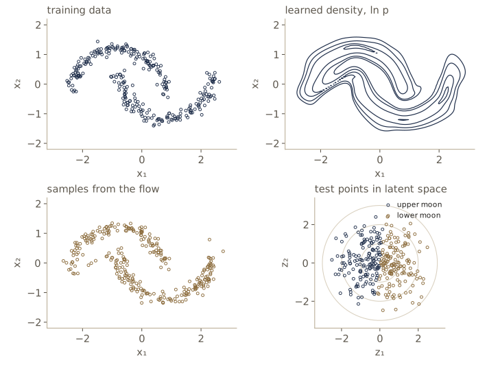
A few things to notice. The test NLL has come down from the Gaussian’s 2.84 nats to within about 0.06 nats of the entropy floor. The latent images of the test points have a mean near zero and a covariance near the identity, as they must if the model is good. Samples score lower under the true density than real data do (an average of −1.90 against −1.67), because some of them fall in the gap between the moons.
That gap is not an accident of training. A flow is a continuous bijection of the plane, so it cannot tear the single connected blob of the Gaussian into two separate pieces; it can only stretch a thin, low-density bridge between them. Increasing the depth makes the bridge thinner but never removes it, which is one reason flows need many layers for multimodal data. A GPU, more layers, wider conditioners, and longer training would bring the NLL closer still to the floor.
Coupling functions and conditioners
Real NVP is one member of a larger family. A general coupling flow replaces the affine map by
\[\mathbf{x}_B = \mathbf{h}\bigl(\mathbf{z}_B, \boldsymbol{\theta}(\mathbf{z}_A, \mathbf{w})\bigr),\]where the coupling function \(\mathbf{h}(\cdot, \boldsymbol{\theta})\) is invertible in its first argument for every value of its parameters \(\boldsymbol{\theta}\), and the conditioner \(\boldsymbol{\theta}(\mathbf{z}_A, \mathbf{w})\) is a neural network that computes those parameters from the copied block. (Bishop & Bishop write the conditioner as \(\mathbf{g}\); we use \(\boldsymbol{\theta}\) to keep \(\mathbf{g}\) for the inverse map.) The triangular argument above goes through unchanged: the Jacobian’s diagonal comes from \(\partial \mathbf{h} / \partial \mathbf{z}_B\) alone.
Common choices, in increasing flexibility:
- Additive coupling, \(\mathbf{x}_B = \mathbf{z}_B + \mathbf{b}(\mathbf{z}_A)\), used by NICE (Dinh, Krueger, and Bengio). Its log-determinant is zero, so the map preserves volume; a final learned diagonal scaling is needed to change volume at all.
- Affine coupling, as above (real NVP, Glow).
- Monotone nonlinear coupling, where each coordinate of \(\mathbf{z}_B\) passes through a strictly increasing scalar function whose shape the conditioner sets, for example a monotone rational-quadratic spline (neural spline flows). One such layer can bend a single coordinate far more than an affine map can, and inversion is still elementwise.
Whatever the choice, the cost of a layer is one pass of the conditioner in either direction, which is why coupling flows are equally fast for density evaluation and for sampling.
Autoregressive flows
From the product rule to a flow
Any joint density can be factorized with the product rule once we fix an ordering of the variables:
\[p(x_1, \dots, x_D) = \prod_{i=1}^{D} p(x_i \mid \mathbf{x}_{1:i-1}),\]where \(\mathbf{x}_{1:i-1} = (x_1, \dots, x_{i-1})\). This is the autoregressive factorization behind the language models of module 12 and the structured models of module 11. Turning it into a flow means generating each coordinate from its own latent variable, with parameters that depend on the coordinates generated before it. A masked autoregressive flow (MAF; Papamakarios, Pavlakou, and Murray) uses
\[x_i = h\bigl(z_i, \boldsymbol{\theta}_i(\mathbf{x}_{1:i-1}, \mathbf{w})\bigr), \qquad z_i = h^{-1}\bigl(x_i, \boldsymbol{\theta}_i(\mathbf{x}_{1:i-1}, \mathbf{w})\bigr),\]and in the affine case \(h(z, (\mu, \alpha)) = \mu + e^{\alpha} z\), so that
\[x_i = \mu_i(\mathbf{x}_{1:i-1}) + e^{\alpha_i(\mathbf{x}_{1:i-1})}\, z_i, \qquad z_i = \bigl(x_i - \mu_i(\mathbf{x}_{1:i-1})\bigr)\, e^{-\alpha_i(\mathbf{x}_{1:i-1})}.\]With Gaussian \(z_i\), the conditional \(p(x_i \mid \mathbf{x}_{1:i-1})\) is the Gaussian \(\mathcal{N}(\mu_i, e^{2\alpha_i})\); stacking several such layers makes the conditionals non-Gaussian.
The Jacobian of the density direction is triangular for the same reason as before. The latent \(z_i\) depends on \(x_i\) and on earlier coordinates only, so \(\partial z_i / \partial x_j = 0\) for \(j > i\): row \(i\) has nonzero entries only up to the diagonal, a lower-triangular matrix. The diagonal entries are \(\partial z_i / \partial x_i = e^{-\alpha_i}\), so
\[\ln \bigl\lvert \det \mathbf{J} \bigr\rvert = -\sum_{i=1}^{D} \alpha_i(\mathbf{x}_{1:i-1}).\]Masks that enforce the ordering: MADE
We could build \(D\) separate conditioner networks, one per coordinate, but that wastes computation. The word “masked” refers to a better idea (Germain, Gregor, Murray, and Larochelle, “MADE”): a single network that outputs all the \(\mu_i\) and \(\alpha_i\) at once, with some weights forced to zero by fixed binary masks so that output \(i\) cannot see inputs \(i, i+1, \dots, D\).
The construction assigns every unit a degree. Input \(x_j\) has degree \(j\). Each hidden unit gets a degree \(m\) between \(1\) and \(D - 1\), meaning it may depend on inputs \(1, \dots, m\) only. A connection from a unit of degree \(m\) into a hidden unit of degree \(m'\) is allowed when \(m' \ge m\), so dependencies can only stay the same or widen as they move up. The output for coordinate \(i\) has degree \(i\) and accepts connections only from hidden units of degree strictly less than \(i\). By induction over layers, every path from \(x_j\) to output \(i\) passes through degrees at least \(j\) and strictly below \(i\), so \(j < i\) is required, which is exactly the autoregressive constraint. Output 1 receives no connections at all: its \(\mu_1\) and \(\alpha_1\) are learned constants, and input \(x_D\) is never used.
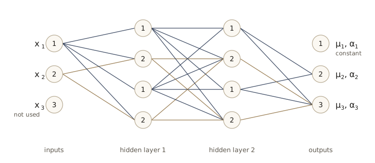
A masked linear layer multiplies its weight matrix elementwise by the mask before using it. Gradients of the masked-out weights are zero, so they never change.
class MaskedLinear(nn.Linear):
    """A linear layer whose weight matrix is multiplied by a fixed 0/1 mask."""
    def __init__(self, n_in, n_out, mask):
        super().__init__(n_in, n_out)
        self.register_buffer("mask", mask.float())

    def forward(self, u):
        return F.linear(u, self.weight * self.mask, self.bias)

def made_masks(D, hidden_sizes):
    """Degrees: inputs 1..D, hidden units cycle through 1..D-1, outputs 1..D."""
    degrees = [torch.arange(1, D + 1)]
    for H in hidden_sizes:
        degrees.append(torch.arange(H) % max(D - 1, 1) + 1)
    masks = [degrees[l + 1][:, None] >= degrees[l][None, :] for l in range(len(hidden_sizes))]
    masks.append(degrees[0][:, None] > degrees[-1][None, :])      # output i sees degrees < i
    return masks, degrees

class MADE(nn.Module):
    """Outputs mu_i and alpha_i that depend only on u_1, ..., u_{i-1}."""
    def __init__(self, D, hidden_sizes):
        super().__init__()
        masks, _ = made_masks(D, hidden_sizes)
        sizes = [D] + list(hidden_sizes)
        layers = []
        for l in range(len(hidden_sizes)):
            layers += [MaskedLinear(sizes[l], sizes[l + 1], masks[l]), nn.Tanh()]
        layers.append(MaskedLinear(sizes[-1], 2 * D, masks[-1].repeat(2, 1)))
        self.net = nn.Sequential(*layers)
        self.passes = 0                              # counts network evaluations

    def forward(self, u):
        self.passes += 1
        mu, alpha = self.net(u).chunk(2, dim=1)
        return mu, torch.tanh(alpha)

torch.manual_seed(4)
made = MADE(5, [16, 16])
u0 = torch.randn(5)
J_mu = torch.autograd.functional.jacobian(lambda v: made(v[None])[0][0], u0)
print("nonzero pattern of d mu_i / d u_j:\n", (J_mu.abs() > 0).int().numpy())
nonzero pattern of d mu_i / d u_j:
 [[0 0 0 0 0]
 [1 0 0 0 0]
 [1 1 0 0 0]
 [1 1 1 0 0]
 [1 1 1 1 0]]
The derivative of each \(\mu_i\) with respect to the inputs is nonzero only strictly below the diagonal, as designed. Although the masks remove many weights, a single MADE is still one ordinary forward pass: all \(D\) conditionals are computed in parallel.
The masked autoregressive flow layer
A MAF layer wraps a MADE. The density direction g computes all the \(z_i\) from one pass over \(\mathbf{x}\), because every \(\mu_i\) and \(\alpha_i\) depends only on observed coordinates. The sampling direction f cannot do that: \(\mu_2\) depends on \(x_1\), which has to be generated first, then \(\mu_3\) on \(x_1\) and \(x_2\), and so on. Sampling is a loop of \(D\) passes, each of which fixes one more coordinate.
class MAFLayer(nn.Module):
    """x_i = mu_i(x_<i) + exp(alpha_i(x_<i)) z_i."""
    def __init__(self, D, hidden_sizes):
        super().__init__()
        self.made, self.D = MADE(D, hidden_sizes), D

    def g(self, x):                                  # density: one pass
        mu, alpha = self.made(x)
        return (x - mu) * torch.exp(-alpha), -alpha.sum(dim=1)

    def f(self, z):                                  # sampling: D passes, one coordinate each
        x = torch.zeros_like(z)
        for i in range(self.D):
            mu, alpha = self.made(x)
            x = x.clone()
            x[:, i] = mu[:, i] + torch.exp(alpha[:, i]) * z[:, i]
        return x, alpha.sum(dim=1)

torch.manual_seed(4)
maf = MAFLayer(5, [16, 16])
x = torch.randn(4, 5)
z, logdet = maf.g(x)
x_back, _ = maf.f(z)
print(f"max abs error of f(g(x)) - x   {(x_back - x).abs().max().item():.1e}")
J = torch.autograd.functional.jacobian(lambda v: maf.g(v[None])[0][0], x[0])
print("Jacobian dz/dx:\n", J.numpy())
print(f"ln|det J|: autograd + slogdet {torch.linalg.slogdet(J)[1].item():.6f}"
      f"   layer's -sum(alpha) {logdet[0].item():.6f}")
max abs error of f(g(x)) - x   1.2e-07
Jacobian dz/dx:
 [[ 0.8792  0.      0.      0.      0.    ]
 [-0.0065  0.7942  0.      0.      0.    ]
 [-0.0122 -0.0291  0.812   0.      0.    ]
 [ 0.0035  0.0619  0.0096  0.8183  0.    ]
 [-0.0193 -0.0473 -0.0237  0.0072  0.8476]]
ln|det J|: autograd + slogdet -0.933275   layer's -sum(alpha) -0.933275
The sequential loop in f works because at iteration \(i\) the first \(i - 1\) coordinates of x are already final, and output \(i\) of the MADE depends only on them; later coordinates, still zero, are invisible to it. The Jacobian is lower triangular and its log-determinant is the sum of the \(-\alpha_i\).
Inverse autoregressive flows
Swapping which variables the conditioner reads gives the inverse autoregressive flow (IAF; Kingma and coauthors):
\[x_i = \mu_i(\mathbf{z}_{1:i-1}) + e^{\alpha_i(\mathbf{z}_{1:i-1})}\, z_i .\]Now the scales and shifts depend on earlier latent coordinates, which are all known when we sample, so sampling is one MADE pass. Evaluating the density of a given \(\mathbf{x}\) is the sequential operation: \(z_1\) comes from \(x_1\) alone, then \(z_2\) needs \(z_1\), and so on. The two flows are the same computation run in opposite directions, which is where the name comes from. For the IAF the forward Jacobian \(\mathbf{K}\) is lower triangular with diagonal \(e^{\alpha_i}\), so \(\ln\lvert\det\mathbf{K}\rvert = \sum_i \alpha_i\).
class IAFLayer(nn.Module):
    """x_i = mu_i(z_<i) + exp(alpha_i(z_<i)) z_i."""
    def __init__(self, D, hidden_sizes):
        super().__init__()
        self.made, self.D = MADE(D, hidden_sizes), D

    def f(self, z):                                  # sampling: one pass
        mu, alpha = self.made(z)
        return mu + torch.exp(alpha) * z, alpha.sum(dim=1)

    def g(self, x):                                  # density: D passes
        z = torch.zeros_like(x)
        for i in range(self.D):
            mu, alpha = self.made(z)
            z = z.clone()
            z[:, i] = (x[:, i] - mu[:, i]) * torch.exp(-alpha[:, i])
        return z, -alpha.sum(dim=1)

torch.manual_seed(4)
iaf = IAFLayer(5, [16, 16])
z = torch.randn(4, 5)
x, logdet_K = iaf.f(z)
z_back, logdet_J = iaf.g(x)
print(f"max abs error of g(f(z)) - z   {(z_back - z).abs().max().item():.1e}")
print("ln q(x) from the sampling pass ", (base_log_prob(z) - logdet_K).detach().numpy())
print("ln q(x) from the density loop  ", (base_log_prob(z_back) + logdet_J).detach().numpy())
max abs error of g(f(z)) - z   2.4e-07
ln q(x) from the sampling pass  [-6.4408 -6.7072 -8.3103 -9.8954]
ln q(x) from the density loop   [-6.4408 -6.7072 -8.3103 -9.8954]
The last two lines show the property that makes the IAF useful: when the model scores its own samples, it already knows the \(\mathbf{z}\) that produced them, so the log density comes out of the one-pass sampling computation, \(\ln q(\mathbf{x}) = \ln p_{\mathbf{z}}(\mathbf{z}) - \ln\lvert\det\mathbf{K}\rvert\), and agrees with the slow loop. That is exactly what variational inference needs: the ELBO of module 19 requires samples from the approximate posterior and their log densities, never the density of an arbitrary external point. The IAF was introduced as a flexible posterior for variational autoencoders for this reason.
The cost asymmetry, measured
We count MADE passes and time both directions of each flow on a batch of 256 vectors in \(D = 64\) dimensions.
D = 64
torch.manual_seed(5)
maf64, iaf64 = MAFLayer(D, [256, 256]), IAFLayer(D, [256, 256])
batch = torch.randn(256, D)
jobs = [("MAF density (g)", maf64, maf64.g), ("MAF sampling (f)", maf64, maf64.f),
        ("IAF density (g)", iaf64, iaf64.g), ("IAF sampling (f)", iaf64, iaf64.f)]
for name, layer, fn in jobs:
    layer.made.passes = 0
    t0 = time.perf_counter()
    with torch.no_grad():
        fn(batch)
    ms = 1000 * (time.perf_counter() - t0)
    print(f"{name:17s} {layer.made.passes:3d} MADE passes   {ms:6.1f} ms")
MAF density (g)     1 MADE passes      1.5 ms
MAF sampling (f)   64 MADE passes     72.7 ms
IAF density (g)    64 MADE passes     74.6 ms
IAF sampling (f)    1 MADE passes      1.8 ms
The pass counts are exact; the times are from one CPU thread and yours will differ, but the slow direction will stay dozens of times slower than the fast one, in line with its 64 passes against one. Neither network is slow in absolute terms. The problem is that the slow direction is inherently sequential: the \(D\) passes cannot run in parallel, so a GPU does not rescue it.
| Flow | Density of a data point | Sampling | Natural use |
|---|---|---|---|
| Coupling (real NVP) | 1 pass | 1 pass | both, with less flexibility per layer |
| Masked autoregressive (MAF) | 1 pass | \(D\) sequential passes | density estimation, maximum likelihood training |
| Inverse autoregressive (IAF) | \(D\) sequential passes | 1 pass (with its own log density) | variational posteriors, fast generation |
Note. A coupling layer is an autoregressive layer with only two groups of variables instead of \(D\): the conditioner for block \(B\) sees all of block \(A\), and block \(A\) gets the identity. It gives up some flexibility per layer to make both directions a single pass. An autoregressive layer is at least as expressive: in two dimensions a MAF layer is exactly a coupling layer plus a learned affine map of the first coordinate, since \(\mu_1\) and \(\alpha_1\) are constants.
Training a MAF on two moons
Since maximum likelihood only ever evaluates densities of data points, MAF trains in single passes. We stack MAF layers with coordinate reversals, as for the coupling flow, and train with the same function.
def maf_flow(n_layers=6, hidden=32, D=2):
    layers = []
    for _ in range(n_layers):
        layers += [MAFLayer(D, [hidden, hidden]), Reverse()]
    return Flow(layers, D=D)

torch.manual_seed(6)
maf_model = maf_flow()
train_flow(maf_model, X_train, steps=1000)
step   250   batch NLL 2.3085   test NLL 2.1853
step   500   batch NLL 1.9278   test NLL 1.9463
step   750   batch NLL 1.8252   test NLL 1.8455
step  1000   batch NLL 1.7835   test NLL 1.8181
The MAF ends at 1.82 nats, a little behind the coupling flow’s 1.73 with fewer layers and fewer training steps. That is no surprise: in two dimensions the two architectures are nearly the same model. The difference between them shows in higher dimensions, where each MAF layer models every conditional of the ordering rather than one split, and where sampling from it gets slow. In practice, MAF-style layers are used for density estimation and IAF-style layers where fast sampling matters; one well-known example trains a fast IAF student to imitate a slow autoregressive teacher so that audio can be generated in parallel.
Continuous flows
Neural ordinary differential equations
Our third construction starts from residual networks. A residual block adds a learned correction to its input, and if all blocks share one set of weights we can write \(\mathbf{z}^{(t+1)} = \mathbf{z}^{(t)} + \mathbf{f}(\mathbf{z}^{(t)}, \mathbf{w})\). Scale the correction by a step size \(h\),
\[\mathbf{z}(t + h) = \mathbf{z}(t) + h\, \mathbf{f}\bigl(\mathbf{z}(t), t, \mathbf{w}\bigr),\]and let \(h \to 0\) while the number of blocks grows like \(T / h\). Rearranging and taking the limit gives an ordinary differential equation for the hidden state,
\[\frac{d\mathbf{z}(t)}{dt} = \mathbf{f}\bigl(\mathbf{z}(t), t, \mathbf{w}\bigr),\]called a neural ODE, short for neural ordinary differential equation (Chen, Rubanova, Bettencourt, and Duvenaud). The network \(\mathbf{f}\) is a vector field: it says in which direction and how fast each point moves. The input is the initial state \(\mathbf{z}(0)\), the output is \(\mathbf{z}(T) = \mathbf{z}(0) + \int_0^T \mathbf{f}(\mathbf{z}(t), t, \mathbf{w})\, dt\), and “depth” has become the continuous variable \(t\), called time. We allowed \(\mathbf{f}\) to depend on \(t\) directly, the continuous analogue of giving each block its own weights. Module 09 made the same observation from the residual-network side: one residual block is one step of Euler’s method.
To compute \(\mathbf{z}(T)\) we need a numerical integrator. Euler’s method is the residual update above; its error after integrating to a fixed time \(T\) shrinks only in proportion to \(h\). The classical fourth-order Runge–Kutta method (RK4) evaluates the field four times per step, at the start, twice at the midpoint, and at the end, and combines them with weights \(\tfrac16, \tfrac13, \tfrac13, \tfrac16\):
\[\begin{aligned} \mathbf{k}_1 &= \mathbf{f}(\mathbf{z}_k, t_k), & \mathbf{k}_2 &= \mathbf{f}\bigl(\mathbf{z}_k + \tfrac{h}{2}\mathbf{k}_1, t_k + \tfrac{h}{2}\bigr), \\ \mathbf{k}_3 &= \mathbf{f}\bigl(\mathbf{z}_k + \tfrac{h}{2}\mathbf{k}_2, t_k + \tfrac{h}{2}\bigr), & \mathbf{k}_4 &= \mathbf{f}(\mathbf{z}_k + h\mathbf{k}_3, t_k + h), \\ \mathbf{z}_{k+1} &= \mathbf{z}_k + \tfrac{h}{6}\bigl(\mathbf{k}_1 + 2\mathbf{k}_2 + 2\mathbf{k}_3 + \mathbf{k}_4\bigr). & & \end{aligned}\]Its error at time \(T\) shrinks like \(h^4\): halving the step divides it by about 16. Our integrator takes fixed steps and runs equally well backward in time (a negative \(h\)), which we will need.
def odeint(f, z0, t0, t1, n_steps, method="rk4"):
    """Integrate dz/dt = f(t, z) from t0 to t1 in n_steps fixed steps (t1 < t0 allowed)."""
    h = (t1 - t0) / n_steps
    z = z0
    for k in range(n_steps):
        t = t0 + k * h
        if method == "euler":
            z = z + h * f(t, z)
        else:
            k1 = f(t, z)
            k2 = f(t + h / 2, z + h / 2 * k1)
            k3 = f(t + h / 2, z + h / 2 * k2)
            k4 = f(t + h, z + h * k3)
            z = z + h / 6 * (k1 + 2 * k2 + 2 * k3 + k4)
    return z

# a test problem with a known answer: a damped rotation dz/dt = A z, so z(T) = exp(AT) z(0)
A = torch.tensor([[-0.1, -1.0], [1.0, -0.1]], dtype=torch.float64)
z_start = torch.tensor([[1.0, 0.0]], dtype=torch.float64)
T_rot = 2 * math.pi
exact = z_start @ torch.linalg.matrix_exp(A * T_rot).T
print(" steps    Euler error    RK4 error")
for n in [10, 20, 40, 80, 160]:
    err = [(odeint(lambda t, z: z @ A.T, z_start, 0.0, T_rot, n, m) - exact).norm().item()
           for m in ["euler", "rk4"]]
    print(f"{n:6d}    {err[0]:.3e}      {err[1]:.3e}")
 steps    Euler error    RK4 error
    10    2.855e+00      4.685e-03
    20    9.026e-01      2.861e-04
    40    3.458e-01      1.766e-05
    80    1.514e-01      1.097e-06
   160    7.089e-02      6.833e-08
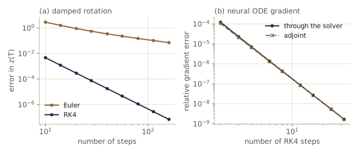
Each doubling of the number of steps divides RK4’s error by about 16, and Euler’s by a factor that settles toward 2 as the steps get small, the fourth- and first-order behavior predicted. For the same accuracy RK4 needs far fewer evaluations of \(\mathbf{f}\), even at four per step.
Practical solvers go further and choose their step sizes adaptively, estimating the local error at each step (for example by comparing a fourth- and a fifth-order formula computed from shared evaluations) and shrinking or growing the step to meet a tolerance. The evaluation times are then not evenly spaced and differ from one input to the next, and the number of function evaluations, which depends on the input and the tolerance, plays the role that depth plays in a layered network. One can also train with a tight tolerance and deploy with a looser one to save computation. We stay with fixed-step RK4, which is easy to reason about and differentiate through.
Backpropagation through a neural ODE
Suppose we have inputs \(\mathbf{z}(0)\), a loss \(L\) that depends on the output \(\mathbf{z}(T)\), and we want \(\nabla_{\mathbf{w}} L\). There are two ways.
Differentiate through the solver (“discretize, then optimize”). The solver is a chain of ordinary tensor operations, and automatic differentiation (module 08) handles it like any deep network. This gives the exact gradient of the discretized computation, but backpropagation must store the intermediate values of every evaluation of \(\mathbf{f}\), so memory grows linearly with the number of steps.
Solve an adjoint equation (“optimize, then discretize”). Derive the continuous-time analogue of backpropagation and integrate it with the solver as a black box. To derive it, go back to the Euler form \(\mathbf{z}_{k+1} = \mathbf{z}_k + h\,\mathbf{f}(\mathbf{z}_k, t_k, \mathbf{w})\) with \(\mathbf{z}_n = \mathbf{z}(T)\), and define the adjoint as the gradient of the loss with respect to the state,
\[\mathbf{a}(t) = \frac{\partial L}{\partial \mathbf{z}(t)} \quad\text{(a column vector)}, \qquad \mathbf{a}_k = \frac{\partial L}{\partial \mathbf{z}_k}.\]The chain rule through one step gives the backward recursion of backpropagation,
\[\mathbf{a}_k = \Bigl(\mathbf{I} + h\,\frac{\partial \mathbf{f}}{\partial \mathbf{z}}\Bigr)^{\mathrm{T}} \mathbf{a}_{k+1} \quad\Longrightarrow\quad \frac{\mathbf{a}_{k+1} - \mathbf{a}_k}{h} = -\Bigl(\frac{\partial \mathbf{f}}{\partial \mathbf{z}}\Bigr)^{\mathrm{T}} \mathbf{a}_{k+1},\]and letting \(h \to 0\) turns it into a differential equation that runs backward from the known final value \(\mathbf{a}(T) = \partial L / \partial \mathbf{z}(T)\):
\[\frac{d\mathbf{a}(t)}{dt} = -\Bigl(\frac{\partial \mathbf{f}}{\partial \mathbf{z}}\bigl(\mathbf{z}(t), t, \mathbf{w}\bigr)\Bigr)^{\mathrm{T}} \mathbf{a}(t).\]For the weights, recall from module 08 that a shared parameter collects the sum of the gradient contributions from every place it is used. The weights are used in every step, and step \(k\) contributes \(h\,(\partial \mathbf{f} / \partial \mathbf{w})^{\mathrm{T}} \mathbf{a}_{k+1}\), so in the limit the sum becomes an integral:
\[\nabla_{\mathbf{w}} L = \int_0^T \Bigl(\frac{\partial \mathbf{f}}{\partial \mathbf{w}}\bigl(\mathbf{z}(t), t, \mathbf{w}\bigr)\Bigr)^{\mathrm{T}} \mathbf{a}(t)\, dt.\]These are the three phases of backpropagation in continuous form: a forward pass for the states, a backward pass for the adjoints, and products of the two for the weight gradients. The matrices \(\partial\mathbf{f}/\partial\mathbf{z}\) and \(\partial\mathbf{f}/\partial\mathbf{w}\) are never formed: each right-hand side is a vector–Jacobian product, which one reverse-mode pass through \(\mathbf{f}\) delivers.
The backward integration needs \(\mathbf{z}(t)\) at whatever times the solver chooses, and storing the forward trajectory would bring back the memory cost. Instead we integrate the state equation backward too, starting from \(\mathbf{z}(T)\), alongside the adjoint. Collect everything into one augmented state \(\bigl(\mathbf{z}, \mathbf{a}, \mathbf{G}\bigr)\) and integrate from \(t = T\) down to \(t = 0\):
\[\frac{d}{dt}\begin{pmatrix} \mathbf{z} \\ \mathbf{a} \\ \mathbf{G} \end{pmatrix} = \begin{pmatrix} \mathbf{f} \\ -(\partial \mathbf{f}/\partial \mathbf{z})^{\mathrm{T}} \mathbf{a} \\ -(\partial \mathbf{f}/\partial \mathbf{w})^{\mathrm{T}} \mathbf{a} \end{pmatrix}, \qquad \begin{pmatrix} \mathbf{z} \\ \mathbf{a} \\ \mathbf{G} \end{pmatrix}\!(T) = \begin{pmatrix} \mathbf{z}(T) \\ \partial L / \partial \mathbf{z}(T) \\ \mathbf{0} \end{pmatrix}.\]Integrating \(d\mathbf{G}/dt\) from \(T\) down to \(0\) gives \(\mathbf{G}(0) = \int_0^T (\partial\mathbf{f}/\partial\mathbf{w})^{\mathrm{T}}\mathbf{a}\,dt = \nabla_{\mathbf{w}} L\).
Watch out. You will see the weight gradient written with a minus sign in front of an integral that runs from \(T\) down to \(0\), or with the adjoint as a row vector and the transposes moved. These are the same formula. Equation (18.26) of Bishop & Bishop carries such a minus sign with limits written from \(0\) to \(T\); read its integral as running in the direction the backward solver runs, from \(T\) down to \(0\). The safe check is the one we do below: compare with backpropagation through the solver on a small problem.
We test both methods on a small neural ODE in double precision: a field with one hidden layer of 32 units, 32 input points, and a squared-error loss against random targets at \(T = 2\). The same field class, with a trace method added later, will define the continuous flow. A saved-tensor hook counts the bytes that autograd stores for the backward pass.
class ODEField(nn.Module):
    """f(z, t) = W2 tanh(W1 [z, t] + b1) + b2: one hidden layer, time as an extra input."""
    def __init__(self, D=2, hidden=64):
        super().__init__()
        self.lin1 = nn.Linear(D + 1, hidden)
        self.lin2 = nn.Linear(hidden, D)

    def forward(self, t, z):
        t_col = torch.full((z.shape[0], 1), float(t), dtype=z.dtype)
        return self.lin2(torch.tanh(self.lin1(torch.cat([z, t_col], dim=1))))

torch.manual_seed(8)
field = ODEField(D=2, hidden=32).double()
params = list(field.parameters())
g8 = torch.Generator().manual_seed(8)
Z0 = torch.randn(32, 2, generator=g8, dtype=torch.float64)
targets = torch.randn(32, 2, generator=g8, dtype=torch.float64)
T_ode = 2.0

def ode_loss(zT):
    return 0.5 * ((zT - targets) ** 2).sum(dim=1).mean()

def saved_bytes(fn):
    """Run fn() and count the bytes autograd saves for the backward pass."""
    total = [0]
    def pack(t):
        total[0] += t.numel() * t.element_size()
        return t
    with torch.autograd.graph.saved_tensors_hooks(pack, lambda t: t):
        out = fn()
    return out, total[0]

def grad_through_solver(n_steps):
    zT, mem = saved_bytes(lambda: odeint(field, Z0, 0.0, T_ode, n_steps))
    grads = torch.autograd.grad(ode_loss(zT), params)
    return torch.cat([g.flatten() for g in grads]), mem

def grad_adjoint(n_steps):
    with torch.no_grad():                            # forward pass: nothing is stored
        zT = odeint(field, Z0, 0.0, T_ode, n_steps)
    zT_leaf = zT.clone().requires_grad_(True)
    aT, = torch.autograd.grad(ode_loss(zT_leaf), zT_leaf)        # a(T) = dL/dz(T)
    B, P = Z0.shape[0], sum(p.numel() for p in params)

    def augmented(t, s):                             # s = (z, a, G) flattened
        z, a = s[:2 * B].view(B, 2), s[2 * B:4 * B].view(B, 2)
        with torch.enable_grad():
            z = z.detach().requires_grad_(True)
            fz = field(t, z)
            # vector-Jacobian products a^T df/dz and a^T df/dw in one reverse pass
            vjps = torch.autograd.grad(fz, [z] + params, grad_outputs=a)
        return torch.cat([fz.flatten()] + [-v.flatten() for v in vjps])

    s_T = torch.cat([zT.flatten(), aT.flatten(), torch.zeros(P, dtype=torch.float64)])
    s_0 = odeint(augmented, s_T, T_ode, 0.0, n_steps)                # integrate back to t = 0
    z0_error = (s_0[:2 * B].view(B, 2) - Z0).abs().max().item()
    return s_0[4 * B:], z0_error

g_ref, _ = grad_through_solver(400)                  # a very accurate reference gradient
rel = lambda u, v: ((u - v).norm() / v.norm()).item()
print(" steps   through solver   adjoint    adjoint vs solver   z(0) error   stored by autograd")
for n in [2, 4, 8, 16, 32]:
    g_direct, mem = grad_through_solver(n)
    g_adj, z0_err = grad_adjoint(n)
    print(f"{n:6d}   {rel(g_direct, g_ref):.2e}         {rel(g_adj, g_ref):.2e}   "
          f"{rel(g_adj, g_direct):.2e}            {z0_err:.1e}      {mem / 1024:7.0f} KiB")
 steps   through solver   adjoint    adjoint vs solver   z(0) error   stored by autograd
     2   1.23e-04         1.07e-04   8.35e-05            2.8e-05          143 KiB
     4   7.12e-06         6.61e-06   4.92e-06            8.7e-07          287 KiB
     8   4.33e-07         4.16e-07   3.01e-07            2.7e-08          575 KiB
    16   2.68e-08         2.61e-08   1.87e-08            8.5e-10         1151 KiB
    32   1.67e-09         1.64e-09   1.16e-09            2.7e-11         2303 KiB
The first two columns are relative errors against the reference gradient, and both fall by roughly a factor of 16 per doubling of the step count, the RK4 rate. The two methods do not agree exactly at any finite step count: backpropagation through the solver is the exact gradient of the discrete computation, while the adjoint is an RK4 approximation of the exact gradient of the continuous one, and the state recomputed backward in time is itself only approximately \(\mathbf{z}(0)\) (fifth column). Both converge to the same answer. The memory column is the real difference: backpropagation through the solver stores intermediate values for every step, growing linearly, while the adjoint’s forward pass runs without a graph and its backward pass needs only the current augmented state.
As a last check that the reference itself is right, a central finite difference on one weight:
eps, w = 1e-6, params[0]
with torch.no_grad():
    w0 = w[0, 0].item()
    w[0, 0] = w0 + eps
    L_plus = ode_loss(odeint(field, Z0, 0.0, T_ode, 400)).item()
    w[0, 0] = w0 - eps
    L_minus = ode_loss(odeint(field, Z0, 0.0, T_ode, 400)).item()
    w[0, 0] = w0
print(f"finite difference {(L_plus - L_minus) / (2 * eps):.8f}"
      f"   reference gradient {g_ref[0].item():.8f}")
finite difference -0.07714482 reference gradient -0.07714482
In practice. The adjoint method trades memory for computation and accuracy: it roughly doubles the work (a second integration of the state, plus the vector–Jacobian products) and relies on the backward integration of \(\mathbf{z}\) being accurate, which can fail when the dynamics are strongly contracting, since running them backward then amplifies errors. Many implementations therefore offer both, and hybrids that store a few checkpoints. If the loss depends on the state at several intermediate times, as with irregularly sampled time series, the backward solve is split at those times and the adjoint receives a jump at each one.
Neural ODE flows: the instantaneous change of variables
A neural ODE is automatically invertible: to recover \(\mathbf{z}(0)\) from \(\mathbf{z}(T)\), integrate the same equation backward in time. (For a well-behaved field, two trajectories can never meet at the same point at the same time, since from that point on they would have to coincide, so distinct starting points stay distinct.) So a neural ODE can serve as a flow, with no architectural restriction on \(\mathbf{f}\) at all. Put a base density \(p(\mathbf{z}(0))\) on the initial state; the ODE carries it to a density \(p(\mathbf{z}(t))\) at every time and to the model density \(p(\mathbf{z}(T))\) at the output. What we need is how \(\ln p\) changes along a trajectory.
Take one Euler step, \(\mathbf{z}' = \mathbf{z} + h\,\mathbf{f}(\mathbf{z}, t)\). Its Jacobian is \(\mathbf{I} + h\,\mathbf{A}\) with \(\mathbf{A} = \partial\mathbf{f}/\partial\mathbf{z}\), and the change of variables for this one step reads \(\ln p_{t+h}(\mathbf{z}') = \ln p_t(\mathbf{z}) - \ln\lvert\det(\mathbf{I} + h\mathbf{A})\rvert\). Expanding the determinant to first order in \(h\) (every term of the permutation expansion except the product of the diagonal carries at least two off-diagonal factors, each of order \(h\)),
\[\det(\mathbf{I} + h\mathbf{A}) = \prod_i (1 + h A_{ii}) + O(h^2) = 1 + h \operatorname{Tr}(\mathbf{A}) + O(h^2),\]so \(\ln\lvert\det(\mathbf{I} + h\mathbf{A})\rvert = h\operatorname{Tr}(\mathbf{A}) + O(h^2)\). Dividing by \(h\) and letting \(h \to 0\) gives the instantaneous change of variables:
Result. Along a trajectory of \(d\mathbf{z}/dt = \mathbf{f}(\mathbf{z}(t), t, \mathbf{w})\), the log density satisfies
\[\frac{d \ln p\bigl(\mathbf{z}(t)\bigr)}{dt} = -\operatorname{Tr}\Bigl(\frac{\partial \mathbf{f}}{\partial \mathbf{z}(t)}\Bigr),\]and so, for the trajectory that ends at \(\mathbf{z}(T) = \mathbf{x}\),
\[\ln p_{\mathbf{x}}(\mathbf{x}) = \ln p_{\mathbf{z}}\bigl(\mathbf{z}(0)\bigr) - \int_0^T \operatorname{Tr}\Bigl(\frac{\partial \mathbf{f}}{\partial \mathbf{z}(t)}\Bigr) dt.\]
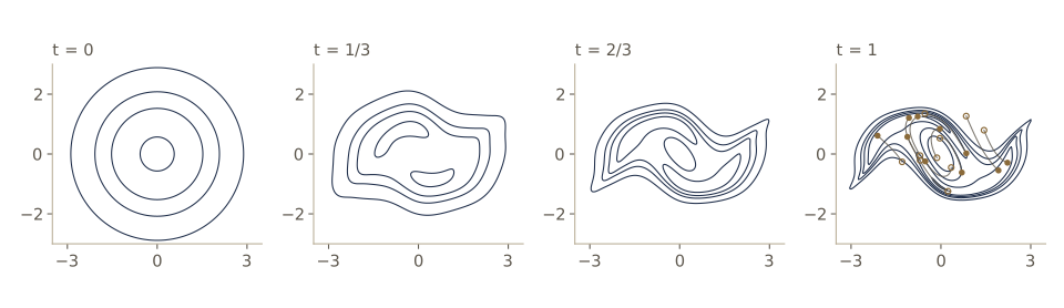
The trace is the divergence of the vector field. Where the flow lines spread apart (positive divergence) probability thins out and the log density falls; where they converge it rises. A model built this way is a continuous normalizing flow. To evaluate the density at a data point we integrate backward from \(\mathbf{x}\) at time \(T\) to time \(0\), carrying the accumulated trace along as one extra coordinate of the state; to sample we integrate forward from a Gaussian draw.
Before building anything we check the formula itself on the untrained field from the adjoint experiment. For one starting point, we integrate the trace along the trajectory, and separately differentiate the whole solver with respect to its starting point and take the log-determinant of that \(2 \times 2\) Jacobian. The trace uses one backward pass per dimension, the exact method for small \(D\).
def trace_autograd(f_val, z, create_graph=False):
    """Exact Tr(df/dz) per row: one reverse-mode pass per dimension."""
    tr = torch.zeros(z.shape[0], dtype=z.dtype)
    for i in range(z.shape[1]):
        grad_i, = torch.autograd.grad(f_val[:, i].sum(), z, create_graph=create_graph,
                                      retain_graph=True)
        tr = tr + grad_i[:, i]
    return tr

def with_trace(t, s):                                # s = (z, c) with dc/dt = +Tr(df/dz)
    with torch.enable_grad():
        z = s[:, :2].detach().requires_grad_(True)
        fz = field(t, z)
        tr = trace_autograd(fz, z)
    return torch.cat([fz, tr[:, None]], dim=1)

z_a = torch.tensor([0.3, -0.7], dtype=torch.float64)
s_T = odeint(with_trace, torch.cat([z_a, torch.zeros(1, dtype=torch.float64)])[None],
             0.0, T_ode, 200)
J_solver = torch.autograd.functional.jacobian(
    lambda v: odeint(field, v[None], 0.0, T_ode, 200)[0], z_a)
print(f"integral of the trace       {s_T[0, 2].item():.10f}")
print(f"ln|det dz(T)/dz(0)|         {torch.linalg.slogdet(J_solver)[1].item():.10f}")
integral of the trace       -0.0638359954
ln|det dz(T)/dz(0)|         -0.0638359954
The two agree to many digits, so the integral of the trace is the log-determinant of the whole transformation, with no triangular structure anywhere.
Training a continuous normalizing flow
For a network with one hidden layer, the trace has a closed form that is cheaper than \(D\) backward passes. Write \(\mathbf{f} = \mathbf{W}_2 \tanh(\mathbf{W}_1 \mathbf{z} + \mathbf{u}t + \mathbf{b}_1) + \mathbf{b}_2\) with \(\mathbf{W}_1\) the part of the first weight matrix that multiplies \(\mathbf{z}\), and let \(\mathbf{h}\) be the vector of hidden activations. Then \(\partial\mathbf{f}/\partial\mathbf{z} = \mathbf{W}_2 \operatorname{diag}(1 - \mathbf{h}^2)\, \mathbf{W}_1\) and, by the cyclic property of the trace,
\[\operatorname{Tr}\Bigl(\frac{\partial\mathbf{f}}{\partial\mathbf{z}}\Bigr) = \sum_{k} (1 - h_k^2) \sum_{i} (W_1)_{ki} (W_2)_{ik}.\]We add this as a method, check it against the autograd loop, and then define the flow. The flow’s state is \((\mathbf{z}, c)\) with \(dc/dt = -\operatorname{Tr}(\partial\mathbf{f}/\partial\mathbf{z})\): integrating from \((\mathbf{x}, 0)\) at time \(T\) down to \(0\) leaves \(c(0) = \int_0^T \operatorname{Tr}\,dt\), and integrating from \((\mathbf{z}(0), \ln p_{\mathbf{z}}(\mathbf{z}(0)))\) forward leaves the log density of the sample in \(c(T)\).
def forward_and_trace(self, t, z):
    """f(z, t) and its exact trace Tr(df/dz) in closed form."""
    t_col = torch.full((z.shape[0], 1), float(t), dtype=z.dtype)
    h = torch.tanh(self.lin1(torch.cat([z, t_col], dim=1)))
    W1 = self.lin1.weight[:, :z.shape[1]]                  # H x D, the columns that see z
    W2 = self.lin2.weight                                  # D x H
    c = (W1 * W2.T).sum(dim=1)                             # c_k = sum_i (W1)_ki (W2)_ik
    return self.lin2(h), ((1 - h ** 2) * c).sum(dim=1)

ODEField.forward_and_trace = forward_and_trace

z_check = torch.randn(5, 2, dtype=torch.float64, requires_grad=True)
f_val, tr_closed = field.forward_and_trace(0.4, z_check)
tr_auto = trace_autograd(field(0.4, z_check), z_check)
print("max abs difference, closed form vs autograd trace: "
      f"{(tr_closed - tr_auto).abs().max().item():.1e}")

class CNF(nn.Module):
    """Continuous flow: dz/dt = f(z, t) and d(ln p)/dt = -Tr(df/dz) for t in [0, T]."""
    def __init__(self, field, T=1.0, n_steps=5):
        super().__init__()
        self.field, self.T, self.n_steps = field, T, n_steps

    def augmented(self, t, s):                       # s = (z, c)
        fz, tr = self.field.forward_and_trace(t, s[:, :-1])
        return torch.cat([fz, -tr[:, None]], dim=1)

    def log_prob(self, x, n_steps=None):
        s_T = torch.cat([x, torch.zeros(x.shape[0], 1, dtype=x.dtype)], dim=1)
        s_0 = odeint(self.augmented, s_T, self.T, 0.0, n_steps or self.n_steps)
        return base_log_prob(s_0[:, :-1]) - s_0[:, -1]

    def sample(self, n, gen=None, n_steps=None):
        z0 = torch.randn(n, 2, generator=gen)
        s_0 = torch.cat([z0, base_log_prob(z0)[:, None]], dim=1)
        s_T = odeint(self.augmented, s_0, 0.0, self.T, n_steps or self.n_steps)
        return s_T[:, :-1], s_T[:, -1]               # samples and their log densities
max abs difference, closed form vs autograd trace: 3.5e-17
We train with backpropagation through five RK4 steps, which is twenty evaluations of the field per density evaluation. The model has a single hidden layer of 64 units; its time input lets the field change as the flow proceeds.
torch.manual_seed(3)
cnf = CNF(ODEField(D=2, hidden=64), T=1.0, n_steps=5)
print("parameters:", sum(p.numel() for p in cnf.parameters()))
train_flow(cnf, X_train, steps=500)
parameters: 386
step   125   batch NLL 2.2199   test NLL 2.1157
step   250   batch NLL 1.9401   test NLL 1.9313
step   375   batch NLL 1.8478   test NLL 1.8912
step   500   batch NLL 1.9075   test NLL 1.8863
The continuous flow gets most of the way from the Gaussian (2.84 nats) toward the floor (1.67) with only 386 parameters, though it trails the coupling flow’s 1.73 here; a deeper field, more steps, and longer training, as in FFJORD (Grathwohl and coauthors), do much better, at a cost a GPU makes bearable. Three checks tell us the density is a real density. It should integrate to one over the plane. Its value should not depend much on how finely we integrate, since the trained object is supposed to approximate a continuous flow. And sampling forward and evaluating backward should agree.
with torch.no_grad():
    g1, g2 = torch.linspace(-4, 4, 161), torch.linspace(-3, 3, 121)
    G1, G2 = torch.meshgrid(g1, g2, indexing="ij")
    grid = torch.stack([G1.flatten(), G2.flatten()], dim=1)
    dens = cnf.log_prob(grid).exp().view(161, 121)
    mass = torch.trapezoid(torch.trapezoid(dens, g2, dim=1), g1).item()
    print(f"integral of the CNF density over the grid   {mass:.4f}")
    for n in [5, 10, 40]:
        nll = -cnf.log_prob(X_test, n).mean().item()
        print(f"test NLL with {n:2d} RK4 steps               {nll:.4f}")
    x_s, logp_forward = cnf.sample(5, gen=torch.Generator().manual_seed(11))
    logp_backward = cnf.log_prob(x_s)
print("ln p of samples, carried forward :", logp_forward.numpy())
print("ln p of samples, evaluated back  :", logp_backward.numpy())
integral of the CNF density over the grid   1.0002
test NLL with  5 RK4 steps               1.8863
test NLL with 10 RK4 steps               1.8866
test NLL with 40 RK4 steps               1.8866
ln p of samples, carried forward : [-2.3208 -1.5567 -1.182  -2.1497 -2.048 ]
ln p of samples, evaluated back  : [-2.3191 -1.5568 -1.1822 -2.1502 -2.0471]
All three checks pass. The density integrates to 1.0002 over the box, within the accuracy of the trapezoid rule on this grid. The test NLL moves by only 0.0003 nats when we integrate with 10 or 40 steps instead of the 5 used in training, so five RK4 steps already solve this smooth field’s ODE accurately: what we trained behaves like a continuous flow, not like a five-layer network that happens to be evaluated with a solver. The log densities carried forward during sampling and those recomputed by integrating backward agree to about \(2 \times 10^{-3}\), the discretization error of five steps in each direction.
Why a trace, and Hutchinson’s estimator
The instantaneous formula trades a determinant for a trace. That looks like a big saving, \(O(D)\) to add a diagonal against \(O(D^3)\) for a general determinant, but the comparison is subtler. Our discrete flows never computed a general determinant either; their triangular Jacobians gave the determinant in \(O(D)\) from quantities the forward pass already produced. The real gain of the continuous flow is freedom: \(\mathbf{f}\) can be any network, with no coupling split, no masks, and no ordering. The catch is that for a general network the diagonal of \(\partial\mathbf{f}/\partial\mathbf{z}\) is not available from one pass. The loop in trace_autograd needs \(D\) backward passes, each costing about one evaluation of \(\mathbf{f}\), which is too slow for images. (Our closed form works only because the field has a single hidden layer.)
Hutchinson’s trace estimator removes the factor \(D\). Let \(\boldsymbol{\epsilon}\) be a random vector with \(\mathbb{E}[\boldsymbol{\epsilon}] = \mathbf{0}\) and \(\mathbb{E}[\boldsymbol{\epsilon}\boldsymbol{\epsilon}^{\mathrm{T}}] = \mathbf{I}\), such as a standard Gaussian or a Rademacher vector with independent entries equal to \(\pm 1\) with probability \(\tfrac12\). Then for any matrix \(\mathbf{A}\),
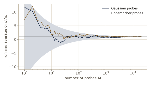
\[\mathbb{E}\bigl[\boldsymbol{\epsilon}^{\mathrm{T}}\mathbf{A}\boldsymbol{\epsilon}\bigr] = \sum_{i,j} A_{ij}\, \mathbb{E}[\epsilon_i \epsilon_j] = \sum_{i,j} A_{ij}\, \delta_{ij} = \operatorname{Tr}(\mathbf{A}),\]so the average \(\frac{1}{M}\sum_{m=1}^{M} \boldsymbol{\epsilon}_m^{\mathrm{T}}\mathbf{A}\boldsymbol{\epsilon}_m\) of \(M\) independent draws is an unbiased estimate of the trace for every \(M\). With \(\mathbf{A} = \partial\mathbf{f}/\partial\mathbf{z}\), the row vector \(\boldsymbol{\epsilon}^{\mathrm{T}}\mathbf{A}\) is a single vector–Jacobian product, one reverse-mode pass, and a dot product with \(\boldsymbol{\epsilon}\) finishes the job. In training one uses \(M = 1\) with a fresh probe for each data point; the extra noise joins the noise of stochastic gradient descent, and the gradient stays unbiased.
The price is variance. Only the symmetric part \(\mathbf{A}_s = \frac12(\mathbf{A} + \mathbf{A}^{\mathrm{T}})\) matters, since \(\boldsymbol{\epsilon}^{\mathrm{T}}\mathbf{A}\boldsymbol{\epsilon} = \boldsymbol{\epsilon}^{\mathrm{T}}\mathbf{A}_s\boldsymbol{\epsilon}\). For Gaussian probes, rotating to the eigenbasis of \(\mathbf{A}_s\) turns the estimate into \(\sum_i \lambda_i \epsilon_i'^2\) with independent \(\epsilon_i'\), whose variance is \(2\sum_i\lambda_i^2 = 2\lVert\mathbf{A}_s\rVert_F^2\). For Rademacher probes \(\epsilon_i^2 = 1\) exactly, the diagonal contributes no noise, and the variance drops to \(2\bigl(\lVert\mathbf{A}_s\rVert_F^2 - \sum_i A_{ii}^2\bigr)\). We check the mean and both variances on the Jacobian of a random network in \(D = 20\), computing all probes in one batched backward pass.
torch.manual_seed(9)
Dh = 20
net20 = nn.Sequential(nn.Linear(Dh, 64), nn.Tanh(), nn.Linear(64, Dh)).double()
with torch.no_grad():
    for p in net20.parameters():
        p.mul_(3.0)                                  # a less trivial Jacobian
z_pt = torch.randn(Dh, dtype=torch.float64)
A_mat = torch.autograd.functional.jacobian(lambda v: net20(v[None])[0], z_pt)
A_sym = 0.5 * (A_mat + A_mat.T)
var_gauss = 2 * (A_sym ** 2).sum().item()
var_rad = 2 * ((A_sym ** 2).sum() - (torch.diagonal(A_mat) ** 2).sum()).item()

def hutchinson_samples(fn, z, M, kind, gen):
    """M single-probe estimates eps^T (df/dz) eps from one batched vector-Jacobian product."""
    Z = z.expand(M, -1).clone().requires_grad_(True)
    if kind == "gaussian":
        eps = torch.randn(Z.shape, generator=gen, dtype=z.dtype)
    else:
        eps = 2.0 * torch.randint(0, 2, Z.shape, generator=gen).to(z.dtype) - 1.0
    eps_A, = torch.autograd.grad(fn(Z), Z, grad_outputs=eps)       # rows eps^T A
    return (eps_A * eps).sum(dim=1)

print(f"exact trace {torch.trace(A_mat).item():.4f}")
M = 20000
for kind, v_theory in [("gaussian", var_gauss), ("rademacher", var_rad)]:
    est = hutchinson_samples(net20, z_pt, M, kind, torch.Generator().manual_seed(9))
    print(f"{kind:10s}  mean of {M} estimates {est.mean().item():.4f} "
          f"(standard error {est.std().item() / math.sqrt(M):.4f})   "
          f"variance {est.var().item():.2f}  vs formula {v_theory:.2f}")
exact trace 0.9740
gaussian    mean of 20000 estimates 0.9623 (standard error 0.0553)   variance 61.11  vs formula 59.67
rademacher  mean of 20000 estimates 1.0059 (standard error 0.0528)   variance 55.80  vs formula 55.99
Both averages sit within one standard error of the exact trace, and the sample variances match the formulas. Here the diagonal of the Jacobian is small, so Rademacher probes help only a little. With a single probe the standard deviation of the estimate is large compared with the trace itself, which is why the estimator is used inside stochastic gradient descent rather than to report a density: for evaluating a trained model on test data one computes the trace exactly, or averages many probes.
Flow matching, and where this leads
Training a continuous flow by maximum likelihood means integrating the ODE, with the trace, at every step, and backpropagating through or around the solver. That is slow and memory-hungry even with the adjoint and Hutchinson’s estimator. Flow matching (Lipman and coauthors) sidesteps the integration during training: it specifies a simple path of densities from the Gaussian to the data, for example by moving each noise sample along a straight line toward a data point, and regresses the network \(\mathbf{f}\) directly onto the velocity of that path, a plain squared-error loss with no solver and no trace. The ODE is only solved at sampling time. This brings continuous flows very close to the diffusion models of module 20, which also learn a vector field by regression and generate by integrating it. There, the deterministic version of the diffusion sampler is itself a continuous normalizing flow, and its exact log likelihood comes from the instantaneous change of variables derived above.
Note. The three families solve the same design problem in different ways. Coupling and autoregressive flows restrict the architecture to make the Jacobian triangular; continuous flows keep the architecture free but pay with an ODE solve and a trace. All of them keep \(\dim\mathbf{z} = \dim\mathbf{x}\) and give exact likelihoods, which is what sets flows apart from GANs, which have no likelihood, and VAEs, which have a bound.
Summary
In the cost column, an entry such as 1 / \(D\) means one network pass to evaluate a density and \(D\) sequential passes to draw a sample.
| Model | Transformation | Log-determinant or density change | Cost |
|---|---|---|---|
| Any flow | \(\mathbf{x} = \mathbf{f}(\mathbf{z})\), \(\mathbf{z} = \mathbf{g}(\mathbf{x})\) | \(\ln\lvert\det\mathbf{J}\rvert = \sum_l \ln\lvert\det\mathbf{J}_l\rvert\) | set by the layers |
| Affine coupling (real NVP) | \(\mathbf{x}_B = e^{\mathbf{s}(\mathbf{z}_A)} \odot \mathbf{z}_B + \mathbf{b}(\mathbf{z}_A)\) | \(\ln\lvert\det\mathbf{K}\rvert = \sum_i s_i\) | 1 / 1 |
| MAF | \(x_i = \mu_i + e^{\alpha_i} z_i\), with \(\mu_i, \alpha_i\) computed from \(\mathbf{x}_{1:i-1}\) | \(\ln\lvert\det\mathbf{J}\rvert = -\sum_i \alpha_i\) | 1 / \(D\) |
| IAF | \(x_i = \mu_i + e^{\alpha_i} z_i\), with \(\mu_i, \alpha_i\) computed from \(\mathbf{z}_{1:i-1}\) | \(\ln\lvert\det\mathbf{K}\rvert = \sum_i \alpha_i\) | \(D\) / 1 |
| Neural ODE | \(d\mathbf{z}/dt = \mathbf{f}(\mathbf{z}, t, \mathbf{w})\) | adjoint: \(d\mathbf{a}/dt = -(\partial\mathbf{f}/\partial\mathbf{z})^{\mathrm{T}}\mathbf{a}\) | one ODE solve each |
| Continuous flow | same ODE, base density at time 0 | \(d\ln p/dt = -\operatorname{Tr}(\partial\mathbf{f}/\partial\mathbf{z})\) | one ODE solve each |
| Hutchinson | \(\operatorname{Tr}(\mathbf{A}) = \mathbb{E}[\boldsymbol{\epsilon}^{\mathrm{T}}\mathbf{A}\boldsymbol{\epsilon}]\) | variance \(2\lVert\mathbf{A}_s\rVert_F^2\) (Gaussian) | one reverse pass per probe |
Ideas to carry forward:
- An invertible network turns a simple density into a complicated one with an exact likelihood; the whole art is in layers whose inverse and log-determinant are cheap. Triangular Jacobians are the recurring trick.
- The direction that needs a sequential loop decides what a flow is good for: MAF for density evaluation and maximum likelihood, IAF for sampling and variational inference, coupling flows for both at some cost in flexibility.
- A residual network is Euler’s method for an ODE. Taking the limit gives neural ODEs, trained either by backpropagating through the solver (exact for the discretization, memory grows with steps) or by the adjoint equations (constant memory, extra computation).
- In continuous time the log-determinant becomes the integral of a trace, which frees the architecture; Hutchinson’s estimator makes the trace affordable, and flow matching, like diffusion, removes the solver from training altogether.
Exercises
- Starting from \(\mathbf{f}(\mathbf{g}(\mathbf{x})) = \mathbf{x}\), show that \(\mathbf{K}\mathbf{J} = \mathbf{I}\) and hence \(\ln p_{\mathbf{x}}(\mathbf{x}) = \ln p_{\mathbf{z}}(\mathbf{z}) - \ln\lvert\det\mathbf{K}\rvert\). Then show that for three layers the inverse is \(\mathbf{g}_1 \circ \mathbf{g}_2 \circ \mathbf{g}_3\) and the log-determinants add. Verify the second claim numerically for a three-layer
Flowin \(D = 3\) usingtorch.autograd.functional.jacobian. - A shift \(\mathbf{x} = \mathbf{z} + \mathbf{b}\) has Jacobian \(\mathbf{I}\). Explain why in terms of volumes. Now take the additive coupling layer \(\mathbf{x}_B = \mathbf{z}_B + \mathbf{b}(\mathbf{z}_A)\) and show it preserves volume even though it is nonlinear. Implement an additive coupling flow for two moons with a final learned diagonal scaling layer, train it with
train_flow, and compare its test NLL with the affine flow’s. What goes wrong without the final scaling? - Remove the \(\tanh\) bound on the log-scales in
AffineCouplingand retrain the coupling flow with learning rates \(10^{-2}\) and \(3 \times 10^{-3}\). Record the largest \(\lvert s_i \rvert\) seen during training and whether the loss stays finite. Explain what you observe. - Replace the fixed
Reverselayers of the coupling flow by learned invertible linear layers \(\mathbf{x} = \mathbf{W}\mathbf{z}\) with \(\mathbf{W} = \mathbf{P}\mathbf{L}\mathbf{U}\) (a fixed permutation, a unit lower-triangular matrix, and an upper-triangular matrix with a positive diagonal parameterized by its logarithm). Derive the log-determinant, implement the layer, check it withslogdet, and compare test NLLs. - Prove that the MADE masks built by
made_masksmake output \(i\) independent of inputs \(j \ge i\), by induction over the layers on the claim “unit of degree \(m\) depends only on inputs \(1, \dots, m\)”. Then show the Jacobian of the MAF density map is lower triangular with diagonal \(e^{-\alpha_i}\). Finally, change the hidden degrees to random integers in \([1, D-1]\) and verify the triangular pattern still holds for \(D = 6\). - Train an IAF (stack
IAFLayers withReverse) to approximate the two-moons density by minimizing the reverse KL divergence \(\mathbb{E}_{q}[\ln q(\mathbf{x}) - \ln p(\mathbf{x})]\), using samples from the IAF andtrue_log_probas the target. Why is the IAF the right choice here and the MAF the wrong one? Report the estimated KL divergence and describe any mode-seeking you see. - Derive the adjoint equation for Euler steps in more detail: write the backward recursion for \(\mathbf{a}_k\) and the weight gradient as a sum over steps, and take the limit. Then extend
grad_adjointto return \(\partial L / \partial \mathbf{z}(0)\) and check it against backpropagation through the solver. - For the damped rotation \(d\mathbf{z}/dt = \mathbf{A}\mathbf{z}\) used to test
odeint, compute \(\operatorname{Tr}(\mathbf{A})\) and predict how the log density of a point changes between \(t = 0\) and \(t = 2\pi\) if \(\mathbf{z}(0)\) is standard Gaussian. Confirm it with the closed-form Gaussian density of \(\mathbf{z}(2\pi) = e^{2\pi\mathbf{A}}\mathbf{z}(0)\). - Derive the one-dimensional instantaneous change of variables \(\frac{d}{dt}\ln p(z(t)) = -f'(z(t))\) directly, by conserving the probability in a small interval that moves with the flow. Illustrate it with \(f(z) = -z\): what happens to a Gaussian of variance 1 as \(t\) grows?
- Show that the Hutchinson estimator with \(M\) probes is unbiased for every \(M\) and that its variance is the single-probe variance divided by \(M\). Derive the Rademacher variance \(2(\lVert\mathbf{A}_s\rVert_F^2 - \sum_i A_{ii}^2)\) by expanding \(\boldsymbol{\epsilon}^{\mathrm{T}}\mathbf{A}_s\boldsymbol{\epsilon}\) and using \(\epsilon_i^2 = 1\). Which probe is better for a diagonal matrix?
- Retrain the continuous flow with a two-hidden-layer field and a Hutchinson trace (one Rademacher probe per point, fresh at each step) instead of the closed form. Evaluate the test NLL with the exact
trace_autogradloop. How do training time and final NLL compare with the one-hidden-layer model? - In your own words: why can a coupling flow sample and evaluate densities equally fast while an autoregressive flow cannot, and what does a continuous flow give up and gain relative to both? Explain it to a classmate who knows the change-of-variables formula but has never seen a flow.
Going further
- C. M. Bishop and H. Bishop, Deep Learning: Foundations and Concepts (Springer, 2024), chapter 18 — the source for this module; free to read at bishopbook.com. Exercises 18.1–18.2 (inverses and determinants of compositions), 18.4 (triangular autoregressive Jacobians), 18.5–18.7 (neural ODEs and their backpropagation as limits of residual networks), 18.8 (the one-dimensional instantaneous change of variables), 18.10 (inverting a continuous flow), and 18.11 (unbiasedness of Hutchinson’s estimator) extend the material here.
- George Papamakarios, Eric Nalisnick, Danilo Jimenez Rezende, Shakir Mohamed, and Balaji Lakshminarayanan, “Normalizing flows for probabilistic modeling and inference,” Journal of Machine Learning Research, 2021, arXiv:1912.02762 — a thorough review of the whole field.
- Laurent Dinh, Jascha Sohl-Dickstein, and Samy Bengio, “Density estimation using Real NVP,” arXiv:1605.08803; George Papamakarios, Theo Pavlakou, and Iain Murray, “Masked autoregressive flow for density estimation,” arXiv:1705.07057; and Diederik P. Kingma and coauthors, “Improved variational inference with inverse autoregressive flow,” arXiv:1606.04934 — the coupling and autoregressive flows of this module.
- Ricky T. Q. Chen, Yulia Rubanova, Jesse Bettencourt, and David Duvenaud, “Neural ordinary differential equations,” arXiv:1806.07366, and Will Grathwohl and coauthors, “FFJORD: Free-form continuous dynamics for scalable reversible generative models,” arXiv:1810.01367 — neural ODEs, the adjoint method, continuous flows, and the Hutchinson trace in training.
- Yaron Lipman and coauthors, “Flow matching for generative modeling,” arXiv:2210.02747 — training continuous flows without a solver.
- Related modules: the change of variables in module 02; backpropagation and shared weights in module 08; residual networks as Euler steps in module 09; the other generative models in module 17, module 19, and module 20; and density estimation with mixtures in Intro to ML, module 09.
These notes follow the chapters of C. M. Bishop and H. Bishop, Deep Learning: Foundations and Concepts (Springer, 2024), the course text, which the authors make free to read online. The explanations, code, figures, and exercises here are written for this course; the book remains the reference, with the full derivations and many more exercises.