CSE 676 · Module 20 · Week 14
Diffusion Models
The noising encoder, the learned reverse decoder and its evidence lower bound, predicting the noise, score matching and stochastic differential equations, and classifier and classifier-free guidance.
Companion reading: Bishop & Bishop, Deep Learning: Foundations and Concepts, chapter 20, “Diffusion Models”
By the end of this module you can
- Define the forward noising chain, derive the diffusion kernel \(q(\mathbf{z}_t \mid \mathbf{x})\) and the Gaussian \(q(\mathbf{z}_{t-1} \mid \mathbf{z}_t, \mathbf{x})\), and check both against simulation.
- Explain why a small noise step makes the reverse step nearly Gaussian, and write down the reverse decoder \(p(\mathbf{z}_{t-1} \mid \mathbf{z}_t, \mathbf{w})\).
- Derive the evidence lower bound of a diffusion model, rewrite it as a sum of Gaussian KL divergences, and reduce it to the noise-prediction loss.
- Train a small denoising network in PyTorch, sample from it with ancestral sampling, and measure the result against the exact data density.
- Relate noise prediction to the score, prove that denoising score matching and explicit score matching differ by a constant, and explain why several noise levels are needed.
- Write the forward process as a stochastic differential equation, sample with the reverse SDE and with the probability-flow ODE, and compute exact log likelihoods from the ODE.
- Implement classifier guidance and classifier-free guidance, and measure how the guidance scale trades diversity for agreement with the label.
Contents
- The forward encoder
- The reverse decoder
- Score matching
- Guided diffusion
- Looking back over the course
- Summary
- Exercises
- Going further
This is the last of the four families of deep generative models in the course. All four share one plan: draw a latent vector from a simple distribution, usually \(\mathcal{N}(\mathbf{0}, \mathbf{I})\), and let a neural network turn it into a data point. Generative adversarial networks (module 17) learn that map with a discriminator as the critic; normalizing flows (module 18) make it invertible so that the likelihood is exact; variational autoencoders (module 19) learn an approximate inverse and train with the evidence lower bound. A diffusion model, also called a denoising diffusion probabilistic model (DDPM), takes yet another route. It never learns the whole map at once. Instead it fixes a long chain that destroys a data point by adding a little Gaussian noise at every step, until nothing but noise is left, and trains one network to undo a single step of that chain. Generation runs the learned undo step many times, starting from pure noise.
That description already contains most of the course. The fixed noising chain is a Markov chain (module 14) that plays the role of a VAE encoder, so a diffusion model is a hierarchical latent-variable model, and the ELBO of module 15 and module 19 is its training objective. Once the bound is simplified, what the network learns is a denoiser, and module 19 showed that a denoiser estimates the score \(\nabla \ln p\), the quantity Langevin sampling needs. Letting the number of steps go to infinity turns the chain into a stochastic differential equation, with a deterministic twin that is a continuous normalizing flow in the sense of module 18. And for images the denoiser is a U-net (module 10).
We build everything on two-dimensional data whose density we know exactly. That is the key to this module’s checks: for a Gaussian mixture, every noisy version of the data is again a Gaussian mixture, so the best possible denoiser, the true score at every noise level, and the true log likelihood are all available in closed form, and we can compare each learned quantity with its exact value. The networks are small enough to train on one CPU thread in about fifteen seconds. We follow Bishop & Bishop chapter 20 section by section and close with a look back over the whole course.
import math
import numpy as np
import torch
import torch.nn as nn
import torch.nn.functional as F

np.set_printoptions(precision=4, suppress=True)
rng = np.random.default_rng(20)
torch.manual_seed(20)
The data set is a spiral with three arms. Each arm is one class and is made of \(J = 4\) elongated Gaussian components laid along a curve, so the density is a mixture of \(K = 12\) Gaussians. The arms have different weights, 0.40, 0.35, and 0.25, which will let us check that a sampler reproduces the proportions of the data and not just its shape. We draw 4,000 training points and 2,000 test points.
C, J = 3, 4                                    # classes (spiral arms), Gaussian components per arm
class_weights = np.array([0.40, 0.35, 0.25])

def spiral_mixture():
    """Means, covariances, log weights and class of each of the C * J mixture components."""
    means, covs, log_w, comp_class = [], [], [], []
    for c in range(C):
        for j in range(J):
            theta, r = 2 * np.pi * c / C + 0.55 * j, 0.55 + 0.42 * j
            radial = np.array([np.cos(theta), np.sin(theta)])
            tangent = 0.42 * radial + 0.55 * r * np.array([-radial[1], radial[0]])
            u = tangent / np.linalg.norm(tangent)
            R = np.stack([u, [-u[1], u[0]]], axis=1)          # columns: along and across the arm
            means.append(r * radial)
            covs.append(R @ np.diag([0.24 ** 2, 0.09 ** 2]) @ R.T)
            log_w.append(np.log(class_weights[c] / J))
            comp_class.append(c)
    as_t = lambda a: torch.tensor(np.array(a), dtype=torch.float32)
    return as_t(means), as_t(covs), as_t(log_w), torch.tensor(comp_class)

mix_mu, mix_cov, mix_logw, comp_class = spiral_mixture()
K = len(mix_mu)

def sample_mixture(n, rng):
    """n points from the mixture, with their class labels."""
    k = rng.choice(K, size=n, p=np.exp(mix_logw.numpy()) / np.exp(mix_logw.numpy()).sum())
    eps = torch.tensor(rng.standard_normal((n, 2)), dtype=torch.float32)
    L = torch.linalg.cholesky(mix_cov)
    return mix_mu[k] + (L[k] @ eps[..., None])[..., 0], comp_class[k]

X, labels = sample_mixture(4000, rng)              # training set, shape (N, D) = (4000, 2)
X_test, labels_test = sample_mixture(2000, rng)
N, D = X.shape
print(f"training data {tuple(X.shape)}, test data {tuple(X_test.shape)}")
print("class fractions:", (torch.bincount(labels) / N).numpy())
print("mean", X.mean(0).numpy(), "  std", X.std(0).numpy())
training data (4000, 2), test data (2000, 2)
class fractions: [0.408  0.3462 0.2457]
mean [-0.0162  0.1414]   std [0.9002 0.9083]
The data are roughly centered with a standard deviation near 1 in each coordinate. That matters: the noising process below pulls everything toward \(\mathcal{N}(\mathbf{0}, \mathbf{I})\), and it does so most gracefully when the data already live on about that scale. For images, the usual preprocessing maps pixel intensities to \([-1, 1]\) for the same reason.
The forward encoder
The forward process takes a data point \(\mathbf{x}\) and produces a sequence of increasingly noisy versions \(\mathbf{z}_1, \mathbf{z}_2, \dots, \mathbf{z}_T\). Each step shrinks the current vector slightly and adds fresh Gaussian noise:
\[\mathbf{z}_t = \sqrt{1 - \beta_t}\, \mathbf{z}_{t-1} + \sqrt{\beta_t}\, \boldsymbol{\epsilon}_t, \qquad \boldsymbol{\epsilon}_t \sim \mathcal{N}(\mathbf{0}, \mathbf{I}),\]with \(\mathbf{z}_0 = \mathbf{x}\). Equivalently, each step is the Gaussian conditional distribution
\[q(\mathbf{z}_t \mid \mathbf{z}_{t-1}) = \mathcal{N}\left(\mathbf{z}_t \mid \sqrt{1 - \beta_t}\, \mathbf{z}_{t-1}, \beta_t \mathbf{I}\right).\]The numbers \(\beta_t \in (0, 1)\) form the noise schedule. They are chosen by hand, not learned, and they usually increase along the chain, \(\beta_1 < \beta_2 < \dots < \beta_T\): early steps remove fine detail gently, later steps can be bolder because little structure is left. The steps form a Markov chain, since \(\mathbf{z}_t\) depends on the past only through \(\mathbf{z}_{t-1}\), and in the language of module 19 the chain is an encoder, one that is fixed rather than learned (figure 1). Note the naming: diffusion papers call this noising direction the forward process, whereas the flows of module 18 call the map from latent to data the forward direction. Many papers also write \(\mathbf{x}_0, \mathbf{x}_1, \dots, \mathbf{x}_T\) where we write \(\mathbf{x}, \mathbf{z}_1, \dots, \mathbf{z}_T\).
Why the factor \(\sqrt{1 - \beta_t}\) in front of \(\mathbf{z}_{t-1}\)? Suppose \(\mathbf{z}_{t-1}\) has mean \(\mathbf{m}\) and covariance \(\mathbf{S}\). Because the noise is independent of \(\mathbf{z}_{t-1}\), means add and covariances add, so \(\mathbf{z}_t\) has mean \(\sqrt{1-\beta_t}\,\mathbf{m}\) and covariance \((1 - \beta_t)\mathbf{S} + \beta_t \mathbf{I}\). The mean shrinks toward zero, the covariance moves a fraction \(\beta_t\) of the way toward \(\mathbf{I}\), and if \(\mathbf{z}_{t-1}\) is already \(\mathcal{N}(\mathbf{0}, \mathbf{I})\) then so is \(\mathbf{z}_t\). The coefficients are chosen precisely so that the standard Gaussian is the fixed point of every step.
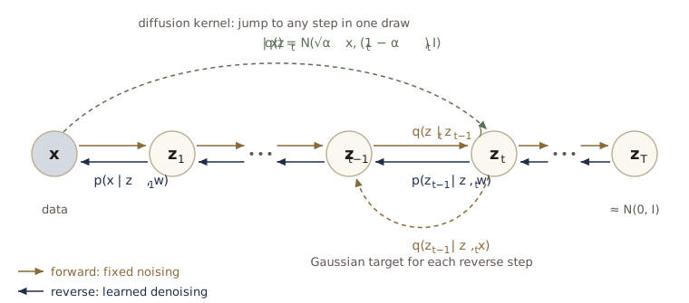
We use \(T = 200\) steps with \(\beta_t\) rising linearly from \(10^{-4}\) to \(0.06\). Image models typically use \(T = 1000\) with smaller steps; our data are simple and two-dimensional, and fewer steps keep sampling cheap. In the code, beta[t] is \(\beta_t\) for \(t = 1, \dots, T\) (the entry beta[0] is a placeholder), so the indices match the math.
T = 200
beta = torch.cat([torch.zeros(1), torch.linspace(1e-4, 0.06, T)]).double()   # beta[t] = beta_t
alpha = torch.cumprod(1 - beta, 0)                         # alpha[t] = prod_{tau <= t} (1 - beta_tau)
for t in [1, 10, 50, 100, 200]:
    signal, noise = alpha[t].sqrt(), (1 - alpha[t]).sqrt()
    print(f"t = {t:3d}   beta_t = {beta[t]:.4f}   alpha_t = {alpha[t]:.4f}   "
          f"signal sqrt(alpha_t) = {signal:.3f}   noise sqrt(1 - alpha_t) = {noise:.3f}")
t =   1   beta_t = 0.0001   alpha_t = 0.9999   signal sqrt(alpha_t) = 1.000   noise sqrt(1 - alpha_t) = 0.010
t =  10   beta_t = 0.0028   alpha_t = 0.9855   signal sqrt(alpha_t) = 0.993   noise sqrt(1 - alpha_t) = 0.120
t =  50   beta_t = 0.0148   alpha_t = 0.6869   signal sqrt(alpha_t) = 0.829   noise sqrt(1 - alpha_t) = 0.560
t = 100   beta_t = 0.0299   alpha_t = 0.2198   signal sqrt(alpha_t) = 0.469   noise sqrt(1 - alpha_t) = 0.883
t = 200   beta_t = 0.0600   alpha_t = 0.0022   signal sqrt(alpha_t) = 0.047   noise sqrt(1 - alpha_t) = 0.999
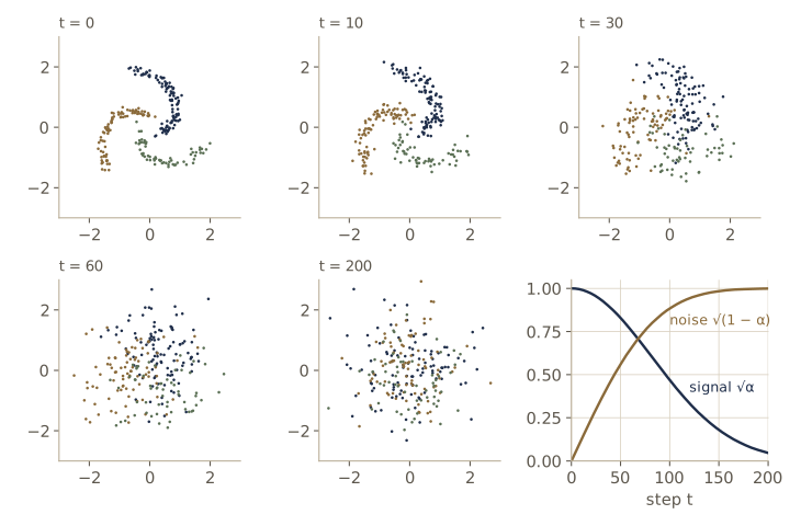
The second array, \(\alpha_t\), is the subject of the next subsection. The two columns on the right tell the story of the chain: after 10 steps the data are only slightly blurred, by \(t = 50\) the noise is already more than half the size of the signal, the two are equal near \(t = 68\), and at \(t = T\) less than 5% of the original signal remains.
The diffusion kernel
To train on step \(t\) we need samples of \(\mathbf{z}_t\), and it would be wasteful to run \(t\) noising steps to get each one. We don’t have to. Conditioned on \(\mathbf{x}\), the chain’s joint distribution is
\[q(\mathbf{z}_1, \dots, \mathbf{z}_t \mid \mathbf{x}) = q(\mathbf{z}_1 \mid \mathbf{x}) \prod_{\tau=2}^{t} q(\mathbf{z}_\tau \mid \mathbf{z}_{\tau-1}),\]and the marginal of the last variable has a closed form. We show by induction that
\[q(\mathbf{z}_t \mid \mathbf{x}) = \mathcal{N}\left(\mathbf{z}_t \mid \sqrt{\alpha_t}\, \mathbf{x}, (1 - \alpha_t)\mathbf{I}\right), \qquad \alpha_t = \prod_{\tau=1}^{t} (1 - \beta_\tau).\]For \(t = 1\) this is the single step itself, since \(\alpha_1 = 1 - \beta_1\). Suppose it holds for \(t - 1\), so that \(\mathbf{z}_{t-1} = \sqrt{\alpha_{t-1}}\,\mathbf{x} + \sqrt{1 - \alpha_{t-1}}\,\boldsymbol{\epsilon}\) with \(\boldsymbol{\epsilon}\) standard normal. One more step gives
\[\mathbf{z}_t = \sqrt{(1 - \beta_t)\alpha_{t-1}}\;\mathbf{x} + \sqrt{1 - \beta_t}\sqrt{1 - \alpha_{t-1}}\;\boldsymbol{\epsilon} + \sqrt{\beta_t}\;\boldsymbol{\epsilon}_t .\]The first coefficient is \(\sqrt{\alpha_t}\). The two noise terms are independent zero-mean Gaussians, so their sum is Gaussian with variance \((1 - \beta_t)(1 - \alpha_{t-1}) + \beta_t = 1 - (1 - \beta_t)\alpha_{t-1} = 1 - \alpha_t\) per coordinate, which completes the induction. This conditional of \(\mathbf{z}_t\) given \(\mathbf{x}\) is called the diffusion kernel. In sampling form,
\[\mathbf{z}_t = \sqrt{\alpha_t}\,\mathbf{x} + \sqrt{1 - \alpha_t}\,\boldsymbol{\epsilon}_t, \qquad \boldsymbol{\epsilon}_t \sim \mathcal{N}(\mathbf{0}, \mathbf{I}),\]where \(\boldsymbol{\epsilon}_t\) is now the total noise accumulated over the first \(t\) steps, not the increment added at step \(t\). Because \(\alpha_t\) is a product of numbers below one, it decreases toward zero, and as \(T \to \infty\) (with the \(\beta_t\) bounded away from zero) \(q(\mathbf{z}_T \mid \mathbf{x}) \to \mathcal{N}(\mathbf{0}, \mathbf{I})\) whatever \(\mathbf{x}\) was. All information about the starting point is gone, so the marginal \(q(\mathbf{z}_T)\) is also standard normal.
Watch out. Much of the diffusion literature (including Ho et al., 2020) writes \(\alpha_t\) for the single-step factor \(1 - \beta_t\) and \(\bar{\alpha}_t\) for the cumulative product. Bishop & Bishop, and these notes, use \(\alpha_t\) for the cumulative product. When you compare formulas with a paper, check which convention it uses first.
We check the kernel by brute force. Starting 50,000 copies of the chain at the same training point and running the noising steps one at a time, the sample mean and covariance of \(\mathbf{z}_t\) should match \(\sqrt{\alpha_t}\,\mathbf{x}\) and \((1 - \alpha_t)\mathbf{I}\).
def forward_step(z, t):
    """One noising step: z_t = sqrt(1 - beta_t) z_{t-1} + sqrt(beta_t) eps_t."""
    return (1 - beta[t]).sqrt() * z + beta[t].sqrt() * torch.randn_like(z)

def diffuse(x, t, eps):
    """Jump straight to step t with the diffusion kernel: sqrt(alpha_t) x + sqrt(1 - alpha_t) eps."""
    return alpha[t].sqrt() * x + (1 - alpha[t]).sqrt() * eps

torch.manual_seed(1)
x0 = X[0].double()
z = x0.repeat(50_000, 1)                      # 50,000 independent chains, all started at the same x
print(f"x = {x0.numpy()}")
for t in range(1, T + 1):
    z = forward_step(z, t)
    if t in (10, 50, 200):
        cov = torch.cov(z.T)
        print(f"t = {t:3d}  chain mean {z.mean(0).numpy()}  "
              f"kernel mean {(alpha[t].sqrt() * x0).numpy()}  chain var {torch.diag(cov).numpy()}  "
              f"kernel var {1 - alpha[t]:.4f}  chain cov {cov[0, 1]:+.4f}")
z_T = diffuse(X.double(), T, torch.randn(N, 2, dtype=torch.float64))
print("whole data set at t = T: mean", z_T.mean(0).numpy(),
      "  covariance", torch.cov(z_T.T).numpy().ravel())
x = [0.5577 1.2633]
t =  10  chain mean [0.5523 1.2542]  kernel mean [0.5537 1.2541]  chain var [0.0145 0.0145]  kernel var 0.0145  chain cov +0.0001
t =  50  chain mean [0.4671 1.0484]  kernel mean [0.4622 1.047 ]  chain var [0.3118 0.3157]  kernel var 0.3131  chain cov -0.0020
t = 200  chain mean [0.021  0.0582]  kernel mean [0.026  0.0588]  chain var [1.0016 0.9908]  kernel var 0.9978  chain cov -0.0006
whole data set at t = T: mean [ 0.0007 -0.0077]   covariance [1.0337 0.0018 0.0018 0.9553]
Mean, variances, and the (zero) covariance all agree to within sampling error, and at \(t = T\) the whole training set has been turned into something indistinguishable, at this sample size, from \(\mathcal{N}(\mathbf{0}, \mathbf{I})\). Figure 2 shows the process on the data set.
Conditional distribution
Generation needs the chain in reverse: given \(\mathbf{z}_t\), what was \(\mathbf{z}_{t-1}\)? Bayes’ theorem gives
\[q(\mathbf{z}_{t-1} \mid \mathbf{z}_t) = \frac{q(\mathbf{z}_t \mid \mathbf{z}_{t-1})\, q(\mathbf{z}_{t-1})}{q(\mathbf{z}_t)}, \qquad q(\mathbf{z}_{t-1}) = \int q(\mathbf{z}_{t-1} \mid \mathbf{x})\, p(\mathbf{x})\, d\mathbf{x},\]and the marginal \(q(\mathbf{z}_{t-1})\) involves the unknown data density. Replacing \(p(\mathbf{x})\) by the training points gives a mixture of \(N\) Gaussians, one per training point, which is neither convenient nor a good model.
If we also condition on the starting point, things become easy. Given \(\mathbf{x}\) the problem is like asking where a random walk was one step ago when we know both where it is now and where it started. By Bayes’ theorem and the Markov property, \(q(\mathbf{z}_t \mid \mathbf{z}_{t-1}, \mathbf{x}) = q(\mathbf{z}_t \mid \mathbf{z}_{t-1})\), so
\[q(\mathbf{z}_{t-1} \mid \mathbf{z}_t, \mathbf{x}) = \frac{q(\mathbf{z}_t \mid \mathbf{z}_{t-1})\, q(\mathbf{z}_{t-1} \mid \mathbf{x})}{q(\mathbf{z}_t \mid \mathbf{x})} .\]Both factors in the numerator are Gaussian in \(\mathbf{z}_{t-1}\), and the denominator does not depend on \(\mathbf{z}_{t-1}\), so the result is Gaussian and we find it by completing the square. Collect the exponent of the numerator as a function of \(\mathbf{z}_{t-1}\):
\[\begin{aligned} &-\frac{\lVert \mathbf{z}_t - \sqrt{1 - \beta_t}\,\mathbf{z}_{t-1} \rVert^2}{2\beta_t} - \frac{\lVert \mathbf{z}_{t-1} - \sqrt{\alpha_{t-1}}\,\mathbf{x} \rVert^2}{2(1 - \alpha_{t-1})} \\ &\qquad = -\frac{1}{2}\left(\frac{1 - \beta_t}{\beta_t} + \frac{1}{1 - \alpha_{t-1}}\right)\lVert \mathbf{z}_{t-1} \rVert^2 \\ &\qquad\quad + \mathbf{z}_{t-1}^{\mathrm{T}}\left(\frac{\sqrt{1 - \beta_t}}{\beta_t}\mathbf{z}_t + \frac{\sqrt{\alpha_{t-1}}}{1 - \alpha_{t-1}}\mathbf{x}\right) + \text{const}. \end{aligned}\]The coefficient of \(-\tfrac12\lVert \mathbf{z}_{t-1} \rVert^2\) is the inverse variance. Over a common denominator it is \(\{(1 - \beta_t)(1 - \alpha_{t-1}) + \beta_t\}/\{\beta_t(1 - \alpha_{t-1})\}\), and we met the numerator in the induction above: it equals \(1 - \alpha_t\). The mean is the variance times the linear coefficient. The result is
Result. The reverse step conditioned on the data point is
\[\begin{aligned} q(\mathbf{z}_{t-1} \mid \mathbf{z}_t, \mathbf{x}) &= \mathcal{N}\left(\mathbf{z}_{t-1} \mid \mathbf{m}_t(\mathbf{x}, \mathbf{z}_t), \sigma_t^2 \mathbf{I}\right), \\ \mathbf{m}_t(\mathbf{x}, \mathbf{z}_t) &= \frac{(1 - \alpha_{t-1})\sqrt{1 - \beta_t}\,\mathbf{z}_t + \sqrt{\alpha_{t-1}}\,\beta_t\,\mathbf{x}}{1 - \alpha_t}, \qquad \sigma_t^2 = \frac{\beta_t (1 - \alpha_{t-1})}{1 - \alpha_t}. \end{aligned}\]The mean is a weighted combination of where we are and where we started; the variance is slightly smaller than \(\beta_t\).
Here \(\alpha_0 = 1\), so \(\sigma_1^2 = 0\): with \(\mathbf{x}\) known, there is nothing uncertain about \(\mathbf{z}_0 = \mathbf{x}\). To check the formula without trusting the algebra, we simulate pairs \((\mathbf{z}_{t-1}, \mathbf{z}_t)\) from the forward process for a fixed \(\mathbf{x}\) and regress \(\mathbf{z}_{t-1}\) on \(\mathbf{z}_t\) by least squares. For jointly Gaussian variables the conditional mean is exactly linear, so the fitted slope and intercept must match the coefficients of \(\mathbf{m}_t\), and the residual variance must match \(\sigma_t^2\).
def posterior(x, z_t, t):
    """Mean m_t(x, z_t) and variance sigma_t^2 of q(z_{t-1} | z_t, x)."""
    m = ((1 - alpha[t - 1]) * (1 - beta[t]).sqrt() * z_t
         + alpha[t - 1].sqrt() * beta[t] * x) / (1 - alpha[t])
    var = beta[t] * (1 - alpha[t - 1]) / (1 - alpha[t])
    return m, var

torch.manual_seed(2)
t = 30
z_prev = diffuse(x0, t - 1, torch.randn(100_000, 2, dtype=torch.float64))   # z_{t-1} ~ q(z_{t-1} | x)
z_t = forward_step(z_prev, t)                                                # z_t ~ q(z_t | z_{t-1})
A = torch.cat([z_t, torch.ones(len(z_t), 1, dtype=torch.float64)], 1)
coef = torch.linalg.lstsq(A, z_prev).solution                               # regress z_{t-1} on [z_t, 1]
resid_var = (z_prev - A @ coef).var(0)
m0, var = posterior(x0, torch.zeros(2, dtype=torch.float64), t)            # intercept = m_t(x, 0)
slope = (1 - alpha[t - 1]) * (1 - beta[t]).sqrt() / (1 - alpha[t])
print(f"slope      regression {coef[0, 0]:.4f} {coef[1, 1]:.4f}   formula {slope:.4f}")
print(f"cross      regression {coef[1, 0]:+.4f} {coef[0, 1]:+.4f}   formula  0")
print(f"intercept  regression {coef[2].numpy()}   formula {m0.numpy()}")
print(f"variance   regression {resid_var.numpy()}   formula {var:.5f}")
slope      regression 0.9334 0.9343   formula 0.9339
cross      regression -0.0003 -0.0010   formula  0
intercept  regression [0.0372 0.0833]   formula [0.0368 0.0833]
variance   regression [0.0083 0.0083]   formula 0.00828
Every coefficient agrees to about three decimals, the accuracy we can expect from 100,000 samples.
For real data, \(q(\mathbf{z}_t)\) is unknown, but for our mixture it is not. Each component \(\mathcal{N}(\boldsymbol{\mu}_k, \boldsymbol{\Sigma}_k)\) pushed through the diffusion kernel becomes \(\mathcal{N}(\sqrt{\alpha_t}\boldsymbol{\mu}_k, \alpha_t\boldsymbol{\Sigma}_k + (1 - \alpha_t)\mathbf{I})\) (a linear map plus independent Gaussian noise), with the same weight. So we can evaluate the exact noisy density \(q(\mathbf{z}_t)\), its gradient \(\nabla \ln q(\mathbf{z}_t)\), and the probability of each class given a noisy point, at every step. These functions are our ground truth for the rest of the module; the network never sees them.
def mixture_stats(z, a):
    """Exact ln q_t(z), its gradient grad ln q_t(z), and the component responsibilities, where
    q_t = sum_k pi_k N(sqrt(a) mu_k, a Sigma_k + (1 - a) I) and a = alpha_t (a = 1: the data density)."""
    a = float(a)
    L = torch.linalg.cholesky(a * mix_cov + (1 - a) * torch.eye(2))
    diff = z[:, None, :] - math.sqrt(a) * mix_mu                      # (n, K, 2)
    prec_diff = torch.cholesky_solve(diff[..., None], L)[..., 0]      # C_k^{-1} (z - m_k)
    log_det = 2 * torch.log(torch.diagonal(L, dim1=-2, dim2=-1)).sum(-1)
    log_joint = mix_logw - 0.5 * (diff * prec_diff).sum(-1) - 0.5 * log_det - math.log(2 * math.pi)
    resp = torch.softmax(log_joint, 1)
    grad_log_q = -(resp[..., None] * prec_diff).sum(1)
    return torch.logsumexp(log_joint, 1), grad_log_q, resp

def class_posterior(z, a):
    """p(c | z_t) under the exact noisy mixture: the summed responsibilities of each class."""
    return torch.zeros(len(z), C).index_add_(1, comp_class, mixture_stats(z, a)[2])

log_p_test = mixture_stats(X_test, 1.0)[0]
print(f"average log density of the test data under the true p(x): {log_p_test.mean():.4f}")
zc, h, a40 = X_test[:4], 1e-3, alpha[40].item()                     # finite-difference check at t = 40
num = torch.stack([(mixture_stats(zc + h * e, a40)[0] - mixture_stats(zc - h * e, a40)[0]) / (2 * h)
                   for e in torch.eye(2)], 1)
err = (num - mixture_stats(zc, a40)[1]).abs().max()
print(f"largest gradient error vs central differences: {err:.1e}")
average log density of the test data under the true p(x): -1.2794
largest gradient error vs central differences: 2.8e-04
The gradient agrees with central differences to within single-precision rounding. The average log density of the test data, about \(-1.28\) nats, is the best any model of these data can do on average; we will compare samplers and bounds against it.
The reverse decoder
The reverse process undoes the chain one step at a time. Since \(q(\mathbf{z}_{t-1} \mid \mathbf{z}_t)\) is intractable, we learn an approximation \(p(\mathbf{z}_{t-1} \mid \mathbf{z}_t, \mathbf{w})\) with a neural network, and generation starts from \(\mathbf{z}_T \sim \mathcal{N}(\mathbf{0}, \mathbf{I})\) and applies it \(T\) times. What family should \(p\) belong to? When \(\beta_t\) is small the answer is simple: \(q(\mathbf{z}_{t-1} \mid \mathbf{z}_t)\) is nearly Gaussian, with a variance close to \(\beta_t\). The reason is visible in Bayes’ theorem above. As a function of \(\mathbf{z}_{t-1}\), the factor \(q(\mathbf{z}_t \mid \mathbf{z}_{t-1})\) is a narrow Gaussian of width about \(\sqrt{\beta_t}\), and over such a narrow window the smooth factor \(q(\mathbf{z}_{t-1})\) barely changes, so it can only tilt the Gaussian slightly. Expanding \(\ln q(\mathbf{z}_{t-1})\) to first order around \(\mathbf{z}_t\) makes this precise and shows that the tilt shifts the mean by about \(\beta_t \nabla \ln q(\mathbf{z}_t)\) (Exercise 3). When \(\beta_t\) is large, the window covers the structure of \(q(\mathbf{z}_{t-1})\) and the reverse distribution can be far from Gaussian, for example multimodal.
We can measure this in one dimension, where \(q(\mathbf{z}_{t-1} \mid \mathbf{z}_t)\) can be computed on a fine grid for any marginal. We take a three-component mixture as \(q(\mathbf{z}_{t-1})\), compute the exact reverse distribution for ten values of \(z_t\), and report how far it is from the best Gaussian (the one with the same mean and variance), measured by the KL divergence, together with the ratio of its variance to \(\beta_t\).
def normal_pdf(x, m, s):
    return torch.exp(-0.5 * ((x - m) / s) ** 2) / (s * math.sqrt(2 * math.pi))

u = torch.linspace(-6, 6, 12001, dtype=torch.float64)            # grid of z_{t-1} values
du = u[1] - u[0]
q_prev = (torch.tensor([0.5, 0.3, 0.2]) *
          normal_pdf(u[:, None], torch.tensor([-1.5, 0.4, 2.0]), torch.tensor([0.3, 0.25, 0.4]))).sum(1)
for b in [0.5, 0.05, 0.005]:
    kls, ratios = [], []
    for zt in torch.linspace(-2.0, 2.5, 10, dtype=torch.float64):
        post = normal_pdf(zt, math.sqrt(1 - b) * u, math.sqrt(b)) * q_prev    # Bayes' numerator
        post = post / (post.sum() * du)
        mean = (u * post).sum() * du
        var = ((u - mean) ** 2 * post).sum() * du
        log_gauss = -0.5 * (u - mean) ** 2 / var - 0.5 * torch.log(2 * math.pi * var)
        ok = post > 0
        kls.append(((post[ok] * (post[ok].log() - log_gauss[ok])).sum() * du).item())
        ratios.append((var / b).item())
    print(f"beta = {b:5.3f}: KL(q(z_t-1 | z_t) || best Gaussian) at most {max(kls):.4f};  "
          f"variance / beta from {min(ratios):.2f} to {max(ratios):.2f}")
beta = 0.500: KL(q(z_t-1 | z_t) || best Gaussian) at most 0.5192;  variance / beta from 0.23 to 2.04
beta = 0.050: KL(q(z_t-1 | z_t) || best Gaussian) at most 0.2309;  variance / beta from 0.58 to 3.42
beta = 0.005: KL(q(z_t-1 | z_t) || best Gaussian) at most 0.0072;  variance / beta from 0.93 to 1.48
With \(\beta = 0.5\) the reverse distribution is badly non-Gaussian for some \(z_t\), and its variance bears little relation to \(\beta\). With \(\beta = 0.005\) it is Gaussian to within a hundredth of a nat, and its variance is of the order of \(\beta\). The price of small steps is their number: many small steps are needed before \(\mathbf{z}_T\) is close to \(\mathcal{N}(\mathbf{0}, \mathbf{I})\), and each generated sample costs one network evaluation per step.
We therefore model each reverse step as
\[p(\mathbf{z}_{t-1} \mid \mathbf{z}_t, \mathbf{w}) = \mathcal{N}\left(\mathbf{z}_{t-1} \mid \boldsymbol{\mu}(\mathbf{z}_t, \mathbf{w}, t), \beta_t \mathbf{I}\right),\]with a fixed variance \(\beta_t\) and a mean computed by a network \(\boldsymbol{\mu}(\mathbf{z}_t, \mathbf{w}, t)\). The network receives the step \(t\) as an input, so a single set of weights serves all \(T\) steps. (Choosing \(\sigma_t^2\) instead of \(\beta_t\) for the variance is the other common fixed choice, and Nichol and Dhariwal (2021) let the network output the variance as well.) The output must have the same shape as the input, which for images makes the U-net of module 10, with its skip connections between matching resolutions, the standard architecture. The full generative model is a Markov chain running backward,
\[p(\mathbf{x}, \mathbf{z}_1, \dots, \mathbf{z}_T \mid \mathbf{w}) = p(\mathbf{z}_T) \left\{ \prod_{t=2}^{T} p(\mathbf{z}_{t-1} \mid \mathbf{z}_t, \mathbf{w}) \right\} p(\mathbf{x} \mid \mathbf{z}_1, \mathbf{w}),\]with \(p(\mathbf{z}_T) = \mathcal{N}(\mathbf{z}_T \mid \mathbf{0}, \mathbf{I})\) and the last step \(p(\mathbf{x} \mid \mathbf{z}_1, \mathbf{w})\) of the same Gaussian form. Sampling from it is ancestral sampling in the sense of module 14: draw \(\mathbf{z}_T\), then each \(\mathbf{z}_{t-1}\) given the one before.
Our network, for two-dimensional data, is a small residual MLP. The step \(t\) enters through sinusoidal features, the same device as the positional encoding of transformers (module 12): \(\sin\) and \(\cos\) of \(t/T\) at eight geometrically spaced frequencies. The embedding is added inside every residual block, so every layer knows how noisy its input is. (We will actually let the network output a noise estimate rather than \(\boldsymbol{\mu}\) directly; the next subsections explain why, and the two are related by a fixed formula.) The optional class input is for guidance at the end of the module.
def time_embed(t, n_freq=8):
    """Sinusoidal features of the step t (a tensor of shape (B,)); periods from 4T down to T/32."""
    freqs = (math.pi / 2) * 2.0 ** torch.arange(n_freq)
    angles = (t.float() / T)[:, None] * freqs
    return torch.cat([angles.sin(), angles.cos()], 1)

class NoiseNet(nn.Module):
    """g(z, w, t), or g(z, w, t, c) when n_classes > 0: a residual MLP whose step (and class)
    embedding is added inside every block."""
    def __init__(self, hidden=64, n_blocks=2, n_classes=0):
        super().__init__()
        self.n_classes = n_classes
        d_cond = 16 + (16 if n_classes else 0)
        if n_classes:
            self.class_emb = nn.Embedding(n_classes + 1, 16)       # index n_classes means "no label"
        self.inp = nn.Linear(2 + d_cond, hidden)
        self.cond = nn.ModuleList([nn.Linear(d_cond, hidden) for _ in range(n_blocks)])
        self.blocks = nn.ModuleList([nn.Sequential(nn.SiLU(), nn.Linear(hidden, hidden), nn.SiLU(),
                                                   nn.Linear(hidden, hidden)) for _ in range(n_blocks)])
        self.out = nn.Sequential(nn.SiLU(), nn.Linear(hidden, 2))

    def forward(self, z, t, c=None):
        e = time_embed(t)
        if self.n_classes:
            e = torch.cat([e, self.class_emb(c)], 1)
        h = self.inp(torch.cat([z, e], 1))
        for cond, block in zip(self.cond, self.blocks):
            h = h + block(h + cond(e))
        return self.out(h)

print("parameters:", sum(p.numel() for p in NoiseNet().parameters()))
parameters: 20162
Training the decoder
The natural objective is the likelihood. For one data point,
\[p(\mathbf{x} \mid \mathbf{w}) = \int \cdots \int p(\mathbf{x}, \mathbf{z}_1, \dots, \mathbf{z}_T \mid \mathbf{w})\, d\mathbf{z}_1 \cdots d\mathbf{z}_T ,\]an integral over every noise trajectory that could have ended at \(\mathbf{x}\). This is the general latent-variable model of module 16 with \(\mathbf{z} = (\mathbf{z}_1, \dots, \mathbf{z}_T)\). Unlike a VAE, every latent vector has the same dimension as the data, as in a normalizing flow. The integral runs through \(T\) nested network evaluations and has no closed form, so, as for the VAE, we maximize a lower bound instead.
The evidence lower bound
For any distribution \(q(\mathbf{z})\) over the latent variables, the log likelihood splits into two parts (module 15):
\[\ln p(\mathbf{x} \mid \mathbf{w}) = \mathcal{L}(\mathbf{w}) + \mathrm{KL}\left(q(\mathbf{z}) \Vert p(\mathbf{z} \mid \mathbf{x}, \mathbf{w})\right), \qquad \mathcal{L}(\mathbf{w}) = \int q(\mathbf{z}) \ln \frac{p(\mathbf{x}, \mathbf{z} \mid \mathbf{w})}{q(\mathbf{z})}\, d\mathbf{z}.\]The identity follows by writing \(p(\mathbf{x}, \mathbf{z} \mid \mathbf{w}) = p(\mathbf{z} \mid \mathbf{x}, \mathbf{w})\, p(\mathbf{x} \mid \mathbf{w})\) inside the logarithm. Since the KL divergence is non-negative, \(\mathcal{L}(\mathbf{w}) \le \ln p(\mathbf{x} \mid \mathbf{w})\): \(\mathcal{L}\) is the evidence lower bound (ELBO). In a VAE, \(q\) is an encoder network trained together with the decoder so that the bound becomes tight. In a diffusion model we make a different choice: \(q\) is the forward process \(q(\mathbf{z}_1, \dots, \mathbf{z}_T \mid \mathbf{x})\), fixed and dependent on \(\mathbf{x}\), and only the reverse model is trained. We give up the chance to tighten the bound through \(q\) and gain a \(q\) that we can sample in one step at any \(t\). This is why a diffusion model is often described as a hierarchical VAE with a fixed encoder (Luo, 2022).
Substituting the two Markov chains,
\[\mathcal{L}(\mathbf{w}) = \mathbb{E}_q\left[ \ln p(\mathbf{z}_T) + \sum_{t=2}^{T} \ln \frac{p(\mathbf{z}_{t-1} \mid \mathbf{z}_t, \mathbf{w})}{q(\mathbf{z}_t \mid \mathbf{z}_{t-1}, \mathbf{x})} - \ln q(\mathbf{z}_1 \mid \mathbf{x}) + \ln p(\mathbf{x} \mid \mathbf{z}_1, \mathbf{w}) \right],\]where \(\mathbb{E}_q\) averages over the forward process started at \(\mathbf{x}\). The first and third terms do not involve \(\mathbf{w}\). The last one is a reconstruction term like the one in a VAE, and it can be estimated by sampling \(\mathbf{z}_1\) from \(q(\mathbf{z}_1 \mid \mathbf{x})\); since \(q\) is fixed, no reparameterization is needed. The sum in the middle is the problem. Each term compares a reverse step with a forward step, and estimating it by sampling a pair \((\mathbf{z}_{t-1}, \mathbf{z}_t)\) gives a noisy estimate. We rewrite it.
Rewriting the ELBO
The trouble is that \(p\) goes backward and \(q\) goes forward. Bayes’ theorem, conditioned on \(\mathbf{x}\), turns the forward step around:
\[\begin{aligned} q(\mathbf{z}_t \mid \mathbf{z}_{t-1}, \mathbf{x}) &= \frac{q(\mathbf{z}_{t-1} \mid \mathbf{z}_t, \mathbf{x})\, q(\mathbf{z}_t \mid \mathbf{x})}{q(\mathbf{z}_{t-1} \mid \mathbf{x})}, \qquad\text{so} \\ \ln \frac{p(\mathbf{z}_{t-1} \mid \mathbf{z}_t, \mathbf{w})}{q(\mathbf{z}_t \mid \mathbf{z}_{t-1}, \mathbf{x})} &= \ln \frac{p(\mathbf{z}_{t-1} \mid \mathbf{z}_t, \mathbf{w})}{q(\mathbf{z}_{t-1} \mid \mathbf{z}_t, \mathbf{x})} + \ln \frac{q(\mathbf{z}_{t-1} \mid \mathbf{x})}{q(\mathbf{z}_t \mid \mathbf{x})} . \end{aligned}\]The last term does not involve \(\mathbf{w}\), and summed over \(t = 2, \dots, T\) it telescopes to \(\ln q(\mathbf{z}_1 \mid \mathbf{x}) - \ln q(\mathbf{z}_T \mid \mathbf{x})\). Its first part cancels the \(-\ln q(\mathbf{z}_1 \mid \mathbf{x})\) above, and its second part combines with \(\ln p(\mathbf{z}_T)\). In each remaining term only two latent variables appear, so all the others integrate out. The result is
Result. The ELBO of a diffusion model is
\[\begin{aligned} \mathcal{L}(\mathbf{w}) = {} & \underbrace{\int q(\mathbf{z}_1 \mid \mathbf{x}) \ln p(\mathbf{x} \mid \mathbf{z}_1, \mathbf{w})\, d\mathbf{z}_1}_{\text{reconstruction}} \\ & - \sum_{t=2}^{T} \underbrace{\int \mathrm{KL}\left(q(\mathbf{z}_{t-1} \mid \mathbf{z}_t, \mathbf{x}) \Vert p(\mathbf{z}_{t-1} \mid \mathbf{z}_t, \mathbf{w})\right) q(\mathbf{z}_t \mid \mathbf{x})\, d\mathbf{z}_t}_{\text{consistency terms}} \\ & - \mathrm{KL}\left(q(\mathbf{z}_T \mid \mathbf{x}) \Vert p(\mathbf{z}_T)\right). \end{aligned}\]The last term has no parameters and is nearly zero when \(\alpha_T \approx 0\); Bishop & Bishop drop it together with the other constants.
Compare this with the VAE bound of module 19: one reconstruction term and one KL term have become one reconstruction term and \(T - 1\) KL terms, one per decoder stage. Each consistency term asks the learned reverse step to match the tractable reverse step \(q(\mathbf{z}_{t-1} \mid \mathbf{z}_t, \mathbf{x})\) from the previous section. And since both are Gaussians with covariances proportional to \(\mathbf{I}\), the KL divergence is available in closed form. For \(\mathcal{N}(\mathbf{m}, \sigma^2\mathbf{I})\) and \(\mathcal{N}(\boldsymbol{\mu}, \beta\mathbf{I})\) in \(D\) dimensions,
\[\mathrm{KL} = \frac{1}{2\beta}\lVert \mathbf{m} - \boldsymbol{\mu} \rVert^2 + \frac{D}{2}\left(\frac{\sigma^2}{\beta} - 1 - \ln\frac{\sigma^2}{\beta}\right),\]and the second part does not depend on \(\mathbf{w}\). So each consistency term is, up to a constant, a squared error between the network’s mean \(\boldsymbol{\mu}(\mathbf{z}_t, \mathbf{w}, t)\) and the target \(\mathbf{m}_t(\mathbf{x}, \mathbf{z}_t)\), averaged over \(\mathbf{z}_t \sim q(\mathbf{z}_t \mid \mathbf{x})\), which we can sample in one draw from the diffusion kernel.
Predicting the noise
Ho et al. (2020) found that a different parameterization of the same network trains better. Instead of the mean, the network predicts the noise. Solve the kernel’s sampling form for the data point, \(\mathbf{x} = (\mathbf{z}_t - \sqrt{1 - \alpha_t}\,\boldsymbol{\epsilon}_t)/\sqrt{\alpha_t}\), and substitute it into \(\mathbf{m}_t\). Using \(\sqrt{\alpha_{t-1}}/\sqrt{\alpha_t} = 1/\sqrt{1 - \beta_t}\), the coefficient of \(\mathbf{z}_t\) becomes \(\{(1 - \alpha_{t-1})(1 - \beta_t) + \beta_t\}/\{\sqrt{1 - \beta_t}(1 - \alpha_t)\} = 1/\sqrt{1 - \beta_t}\), and
\[\mathbf{m}_t(\mathbf{x}, \mathbf{z}_t) = \frac{1}{\sqrt{1 - \beta_t}}\left( \mathbf{z}_t - \frac{\beta_t}{\sqrt{1 - \alpha_t}}\,\boldsymbol{\epsilon}_t \right).\]The target mean is the current point with a scaled copy of the total noise removed. This suggests giving the network the same form, with a network \(\mathbf{g}(\mathbf{z}_t, \mathbf{w}, t)\) that predicts the total noise \(\boldsymbol{\epsilon}_t\) from the noisy point:
\[\boldsymbol{\mu}(\mathbf{z}_t, \mathbf{w}, t) = \frac{1}{\sqrt{1 - \beta_t}}\left( \mathbf{z}_t - \frac{\beta_t}{\sqrt{1 - \alpha_t}}\,\mathbf{g}(\mathbf{z}_t, \mathbf{w}, t) \right).\]Now \(\mathbf{m}_t - \boldsymbol{\mu} = \beta_t(\mathbf{g} - \boldsymbol{\epsilon}_t)/\{\sqrt{1 - \beta_t}\sqrt{1 - \alpha_t}\}\), and each consistency term becomes a weighted squared error on the noise:
\[\begin{aligned} &\mathrm{KL}\left(q(\mathbf{z}_{t-1} \mid \mathbf{z}_t, \mathbf{x}) \Vert p(\mathbf{z}_{t-1} \mid \mathbf{z}_t, \mathbf{w})\right) \\ &\qquad = \frac{\beta_t}{2(1 - \alpha_t)(1 - \beta_t)} \left\lVert \mathbf{g}\left(\sqrt{\alpha_t}\,\mathbf{x} + \sqrt{1 - \alpha_t}\,\boldsymbol{\epsilon}_t, \mathbf{w}, t\right) - \boldsymbol{\epsilon}_t \right\rVert^2 + \text{const}. \end{aligned}\]The reconstruction term turns out to have the same form. With \(\alpha_1 = 1 - \beta_1\) and \(\mathbf{z}_1 = \sqrt{1 - \beta_1}\,\mathbf{x} + \sqrt{\beta_1}\,\boldsymbol{\epsilon}_1\), the formula for \(\boldsymbol{\mu}\) gives \(\mathbf{x} - \boldsymbol{\mu}(\mathbf{z}_1, \mathbf{w}, 1) = \sqrt{\beta_1}(\mathbf{g} - \boldsymbol{\epsilon}_1)/\sqrt{1 - \beta_1}\), so that \(\ln p(\mathbf{x} \mid \mathbf{z}_1, \mathbf{w}) = -\lVert \mathbf{g}(\mathbf{z}_1, \mathbf{w}, 1) - \boldsymbol{\epsilon}_1 \rVert^2 / \{2(1 - \beta_1)\} + \text{const}\), which is the \(t = 1\) case of the same weighted error. Before using these formulas we verify them: the two expressions for \(\mathbf{m}_t\) should agree, the Gaussian KL should agree with PyTorch’s kl_divergence, and the KL should equal the weighted noise error plus the constant, for any network output \(\mathbf{g}\).
from torch.distributions import Normal, Independent, kl_divergence

def mean_from_noise(z_t, t, g):
    """mu(z_t, w, t) from a noise prediction g."""
    return (z_t - beta[t] / (1 - alpha[t]).sqrt() * g) / (1 - beta[t]).sqrt()

def kl_iso(m1, v1, m2, v2):
    """KL( N(m1, v1 I) || N(m2, v2 I) ) in D dimensions (the last axis)."""
    d = m1.shape[-1]
    return 0.5 * (d * (v1 / v2 - 1 - math.log(v1 / v2)) + ((m1 - m2) ** 2).sum(-1) / v2)

torch.manual_seed(3)
x = X[:5].double()
for t in [2, 20, 150]:
    eps = torch.randn_like(x)
    z_t = diffuse(x, t, eps)
    g = eps + 0.3 * torch.randn_like(x)                      # stand-in for an imperfect network output
    m, var = posterior(x, z_t, t)
    m_eps = mean_from_noise(z_t, t, eps)                     # m_t written with the true noise
    mu = mean_from_noise(z_t, t, g)
    kl = kl_iso(m, var, mu, beta[t])
    kl_torch = kl_divergence(Independent(Normal(m, var.sqrt().expand_as(m)), 1),
                             Independent(Normal(mu, beta[t].sqrt().expand_as(mu)), 1))
    weight = beta[t] / (2 * (1 - alpha[t]) * (1 - beta[t]))
    kl_noise = weight * ((g - eps) ** 2).sum(1) + kl_iso(m[:1], var, m[:1], beta[t])   # error + const
    print(f"t = {t:3d}: m_t two ways {(m - m_eps).abs().max():.0e}   "
          f"KL vs torch {(kl - kl_torch).abs().max():.0e}   "
          f"KL vs weighted noise error {(kl - kl_noise).abs().max():.0e}   weight {weight:.4f}")
t =   2: m_t two ways 1e-13   KL vs torch 2e-16   KL vs weighted noise error 2e-12   weight 0.4004
t =  20: m_t two ways 1e-15   KL vs torch 3e-17   KL vs weighted noise error 2e-15   weight 0.0508
t = 150: m_t two ways 2e-16   KL vs torch 6e-17   KL vs weighted noise error 4e-17   weight 0.0243
All three pairs agree to rounding error. The last column shows the ELBO’s weights: they fall steeply with \(t\), so the true bound spends most of its attention on the nearly clean steps. Ho et al. (2020) found that dropping the weights altogether gives better samples, which leads to the simplified loss
\[\mathcal{L}_{\text{simple}}(\mathbf{w}) = \sum_{t=1}^{T} \left\lVert \mathbf{g}\left(\sqrt{\alpha_t}\,\mathbf{x} + \sqrt{1 - \alpha_t}\,\boldsymbol{\epsilon}_t, \mathbf{w}, t\right) - \boldsymbol{\epsilon}_t \right\rVert^2 ,\]to be minimized (the sign flips, since we maximized \(\mathcal{L}\)). It says: take a training point, choose a step, add the corresponding amount of noise, and ask the network what noise was added. The target is the total noise, not the increment of step \(t\). In stochastic gradient descent we do not sum over all \(T\) steps for each point; we pick one step at random per example, which gives an unbiased estimate of the sum, and every time a point is reused it gets fresh noise, a built-in form of data augmentation. Relative to the ELBO, the unweighted loss shifts effort from the smallest \(t\), where the task is nearly impossible (the noise is tiny and almost invisible), toward the larger \(t\) that decide the coarse layout of a sample.
Here is the training loop, which is Algorithm 20.1 of Bishop & Bishop with minibatches. We use Adam with a learning rate that decays linearly to zero (module 07).
def train_ddpm(model, X, labels=None, p_drop=0.0, steps=3000, batch=512, lr=3e-3, log_every=500):
    """Minimize the simplified loss: random x, random t, fresh noise, squared error on the noise.
    With labels, each label is replaced by the null class with probability p_drop (used in guidance)."""
    opt = torch.optim.Adam(model.parameters(), lr=lr, foreach=True)
    sched = torch.optim.lr_scheduler.LambdaLR(opt, lambda s: 1 - s / steps)
    running = []
    for step in range(1, steps + 1):
        idx = torch.randint(0, len(X), (batch,))
        x = X[idx]
        t = torch.randint(1, T + 1, (batch,))                                  # t ~ uniform{1..T}
        eps = torch.randn_like(x)
        z_t = alpha[t].float().sqrt()[:, None] * x + (1 - alpha[t]).float().sqrt()[:, None] * eps
        if labels is None:
            g = model(z_t, t)
        else:
            c = torch.where(torch.rand(batch) < p_drop, model.n_classes, labels[idx])
            g = model(z_t, t, c)
        loss = (g - eps).pow(2).sum(1).mean()
        opt.zero_grad()
        loss.backward()
        opt.step()
        sched.step()
        running.append(loss.item())
        if step % log_every == 0:
            recent = np.mean(running[-log_every:])
            print(f"step {step:5d}   loss (mean of last {log_every}) {recent:.4f}")
    return model

torch.manual_seed(4)
g_net = train_ddpm(NoiseNet(), X)
step   500   loss (mean of last 500) 0.6879
step  1000   loss (mean of last 500) 0.6374
step  1500   loss (mean of last 500) 0.6206
step  2000   loss (mean of last 500) 0.6005
step  2500   loss (mean of last 500) 0.5916
step  3000   loss (mean of last 500) 0.5856
The loss falls quickly and then creeps down. It cannot approach zero: at large \(t\) the noise is almost all of \(\mathbf{z}_t\) and is easy to predict, but at small \(t\) the noise is a tiny perturbation of a data point, and no function of \(\mathbf{z}_t\) can tell exactly which perturbation was added. How good is the network, then? For our data we can compute the best possible predictor. The minimizer of the expected squared error is the conditional mean \(\mathbb{E}[\boldsymbol{\epsilon}_t \mid \mathbf{z}_t]\) (the regression result of module 04), and it has a neat form. Differentiating \(q(\mathbf{z}_t) = \int q(\mathbf{z}_t \mid \mathbf{x})p(\mathbf{x})\,d\mathbf{x}\) under the integral, with \(\nabla \ln q(\mathbf{z}_t \mid \mathbf{x}) = -(\mathbf{z}_t - \sqrt{\alpha_t}\,\mathbf{x})/(1 - \alpha_t) = -\boldsymbol{\epsilon}_t/\sqrt{1 - \alpha_t}\), gives
\[\nabla \ln q(\mathbf{z}_t) = \int \nabla \ln q(\mathbf{z}_t \mid \mathbf{x})\, p(\mathbf{x} \mid \mathbf{z}_t)\, d\mathbf{x} = -\frac{\mathbb{E}[\boldsymbol{\epsilon}_t \mid \mathbf{z}_t]}{\sqrt{1 - \alpha_t}} .\]So the ideal noise predictor is \(-\sqrt{1 - \alpha_t}\,\nabla \ln q(\mathbf{z}_t)\), which mixture_stats gives us exactly. This is Tweedie’s formula from module 19 in a new guise, and we return to it in the section on score matching. We compare the network’s loss with the best achievable loss at several steps, on fresh points from the true density.
def net_eps(net, c=None):
    """Wrap a network as a noise predictor eps_fn(z, t) for an integer step t (and optional class c)."""
    def fn(z, t):
        tt = torch.full((len(z),), t)
        return net(z, tt) if c is None else net(z, tt, torch.full((len(z),), c))
    return fn

def exact_eps(z, t):
    """The best possible noise prediction E[eps | z_t] = -sqrt(1 - alpha_t) grad ln q_t(z_t)."""
    a = alpha[t].item()
    return -math.sqrt(1 - a) * mixture_stats(z, a)[1]

torch.manual_seed(5)
x_eval, _ = sample_mixture(20_000, np.random.default_rng(5))
with torch.no_grad():
    for t in [1, 5, 10, 20, 50, 100, 200]:
        eps = torch.randn_like(x_eval)
        z_t = diffuse(x_eval, t, eps).float()
        loss_net = (net_eps(g_net)(z_t, t) - eps).pow(2).sum(1).mean()
        loss_opt = (exact_eps(z_t, t) - eps).pow(2).sum(1).mean()
        print(f"t = {t:3d}   network {loss_net:.4f}   best possible {loss_opt:.4f}")
t =   1   network 2.0516   best possible 1.9922
t =   5   network 1.7779   best possible 1.7061
t =  10   network 1.4318   best possible 1.3387
t =  20   network 1.2920   best possible 1.2415
t =  50   network 1.2058   best possible 1.2006
t = 100   network 0.3754   best possible 0.3749
t = 200   network 0.0057   best possible 0.0036
From \(t = 50\) on, the network is within about 0.005 of the optimum. At small \(t\) it is several percent worse. There the ideal predictor has to resolve the fine structure of the arms, whose components have a standard deviation of only 0.09 across the arm, and a small network trained for a few seconds does that only approximately. Note also how the best achievable loss depends on \(t\): at \(t = 1\) it is essentially \(D = 2\), the loss of predicting zero, because noise of standard deviation 0.01 cannot be told apart from the data’s own spread.
With the network trained, we can evaluate the full ELBO, constants included, and compare it with the true average log density. The bound must come out below it: in expectation over the data, \(\mathcal{L} \le \ln p(\mathbf{x} \mid \mathbf{w})\), and no model’s average log likelihood can exceed that of the true density (Gibbs’ inequality). We also evaluate the ELBO of the ideal noise predictor, which is the best bound any network of this form could reach, because each consistency term is minimized separately by the conditional mean.
@torch.no_grad()
def elbo(eps_fn, x):
    """One-sample Monte Carlo estimate of the full ELBO for each row of x: reconstruction term,
    consistency terms, and the parameter-free term -KL(q(z_T | x) || N(0, I))."""
    x = x.double()
    eps = torch.randn_like(x)
    z1 = diffuse(x, 1, eps)
    mu = mean_from_noise(z1, 1, eps_fn(z1.float(), 1).double())
    L = -0.5 * ((x - mu) ** 2).sum(1) / beta[1] - 0.5 * D * torch.log(2 * math.pi * beta[1])
    for t in range(2, T + 1):
        z_t = diffuse(x, t, torch.randn_like(x))
        m, var = posterior(x, z_t, t)
        L = L - kl_iso(m, var, mean_from_noise(z_t, t, eps_fn(z_t.float(), t).double()), beta[t])
    L = L - kl_iso(alpha[T].sqrt() * x, 1 - alpha[T], torch.zeros_like(x), torch.tensor(1.0))
    return L

torch.manual_seed(6)
x_b = X_test[:1000]
print(f"true average log density         {mixture_stats(x_b, 1.0)[0].mean():.3f}")
print(f"ELBO, ideal noise predictor      {elbo(exact_eps, x_b).mean():.3f}")
print(f"ELBO, trained network            {elbo(net_eps(g_net), x_b).mean():.3f}")
true average log density         -1.287
ELBO, ideal noise predictor      -1.361
ELBO, trained network            -1.595
Both bounds sit below the true value, as they must. The gap for the ideal predictor is the price of the Gaussian reverse steps with fixed variance \(\beta_t\); the extra gap for the trained network reflects the small-\(t\) errors in the table above.
Generating new samples
Sampling follows the reverse chain (Algorithm 20.2 of Bishop & Bishop). Draw \(\mathbf{z}_T \sim \mathcal{N}(\mathbf{0}, \mathbf{I})\); then, for \(t = T, \dots, 2\), evaluate the network, form the mean \(\boldsymbol{\mu}(\mathbf{z}_t, \mathbf{w}, t)\), and draw
\[\mathbf{z}_{t-1} = \boldsymbol{\mu}(\mathbf{z}_t, \mathbf{w}, t) + \sqrt{\beta_t}\,\boldsymbol{\epsilon}, \qquad \boldsymbol{\epsilon} \sim \mathcal{N}(\mathbf{0}, \mathbf{I}).\]At the last step we output the mean \(\boldsymbol{\mu}(\mathbf{z}_1, \mathbf{w}, 1)\) without adding noise. Notice the bookkeeping: the network estimates the total noise in \(\mathbf{z}_t\), but each step removes only the fraction \(\beta_t/\sqrt{1 - \alpha_t}\) of that estimate, and then fresh noise of variance \(\beta_t\) goes back in. The sample is refined gradually, and early mistakes can be corrected by later steps.
To judge the samples we use two numbers, because each alone can be fooled. The average true log density of the samples, \(\ln p(\mathbf{x})\), rewards samples that land where the data are, but a sampler that piles everything onto the densest spots would score better than real data. The energy distance between the samples and the test set,
\[2\,\mathbb{E}\lVert \mathbf{a} - \mathbf{b} \rVert - \mathbb{E}\lVert \mathbf{a} - \mathbf{a}' \rVert - \mathbb{E}\lVert \mathbf{b} - \mathbf{b}' \rVert ,\]with \(\mathbf{a}, \mathbf{a}'\) independent samples and \(\mathbf{b}, \mathbf{b}'\) independent test points, is zero only when the two distributions are equal, so it also punishes missing spread. We also report the fraction of samples in each class, using the true class posterior, to check the arm weights 0.40, 0.35, 0.25. For reference we score a fresh sample from the true density.
@torch.no_grad()
def sample_ddpm(eps_fn, n, keep=()):
    """Ancestral sampling through the reverse chain; also returns the z_t for the steps listed in keep."""
    z = torch.randn(n, 2)
    snaps = {T: z.clone()}
    for t in range(T, 0, -1):
        mu = mean_from_noise(z, t, eps_fn(z, t)).float()
        z = mu + beta[t].sqrt().float() * torch.randn_like(z) if t > 1 else mu
        if t - 1 in keep:
            snaps[t - 1] = z.clone()
    return z, snaps

def energy_distance(a, b):
    """2 E||a - b|| - E||a - a'|| - E||b - b'||, estimated from two samples."""
    return (2 * torch.cdist(a, b).mean() - torch.cdist(a, a).mean() - torch.cdist(b, b).mean()).item()

def report(name, x, nfe=None):
    lp = mixture_stats(x, 1.0)[0]
    frac = class_posterior(x, 1.0).argmax(1).bincount(minlength=C) / len(x)
    nfe = "" if nfe is None else f"{nfe:4d}"
    print(f"{name:28s} {nfe:>4s}   mean ln p(x) {lp.mean():7.3f}   "
          f"energy distance {energy_distance(x, X_test):.4f}   classes {frac.numpy()}")

torch.manual_seed(7)
x_net, snaps = sample_ddpm(net_eps(g_net), 2000, keep=(100, 50, 20))
torch.manual_seed(7)
x_ideal, _ = sample_ddpm(exact_eps, 2000)
report("fresh sample from p(x)", sample_mixture(2000, np.random.default_rng(7))[0])
report("DDPM, trained network", x_net)
report("DDPM, ideal noise predictor", x_ideal)
fresh sample from p(x)              mean ln p(x)  -1.314   energy distance 0.0006   classes [0.4045 0.3405 0.255 ]
DDPM, trained network               mean ln p(x)  -1.824   energy distance 0.0015   classes [0.405  0.3375 0.2575]
DDPM, ideal noise predictor         mean ln p(x)  -1.358   energy distance 0.0005   classes [0.395 0.339 0.266]
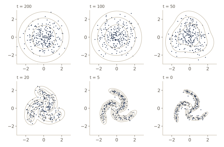
The sampler with the ideal noise predictor is almost indistinguishable from real data, which confirms that 200 Gaussian reverse steps are enough for this problem. The trained network’s samples reproduce the class proportions and have a small energy distance, but their average log density is lower: some samples fall in the gaps between and around the arms, the visible trace of the small-\(t\) errors. Figure 3 shows the samples forming.
In practice. For images the recipe is the same with three changes: a U-net (module 10) with attention layers in place of the MLP, around \(T = 1000\) steps, and far more training (hundreds of thousands of steps on a GPU). Training is stable and needs no adversary, one of the main attractions of diffusion models over the GANs of module 17. The cost moves to sampling: every sample needs one network evaluation per step. Two lines of work reduce it. Song, Meng and Ermon (2020) introduced denoising diffusion implicit models (DDIM), which keep the training objective but use a non-Markovian reverse process that can skip steps, often cutting the number of evaluations by one or two orders of magnitude. And viewing sampling as solving a differential equation (the end of the next section) lets us use better numerical solvers. Diffusion models have also been defined for discrete data, with corruption processes that replace tokens or categories rather than add Gaussian noise (Austin et al., 2021). One use is generating candidate molecules, where the atom types are discrete; there the denoiser works on a graph of atoms, typically a graph network of the kind built in module 13, and when atom positions are generated too, an equivariant one, so that rotating the input rotates the predicted noise.
Score matching
The models so far were derived from a latent-variable model and its ELBO. A second line of work, developed largely independently, arrives at essentially the same algorithm from the direction of energy-based models (module 14). Its central object is the score function, the gradient of the log density with respect to the data vector,
\[\mathbf{s}(\mathbf{x}) = \nabla_{\mathbf{x}} \ln p(\mathbf{x}).\]It is a vector field with one component per input dimension, and it points toward higher density. The gradient is with respect to \(\mathbf{x}\), not with respect to any parameters. Knowing the score means knowing the density up to a constant: if two densities have the same score everywhere, integrating gives \(\ln q = \ln p + \text{const}\), so \(q = Kp\). And the normalizing constant, the bane of energy-based models, disappears under the gradient. Langevin dynamics (module 14) needs nothing but the score to draw samples.
We have in fact been learning scores all along. The identity above, \(\nabla \ln q(\mathbf{z}_t) = -\mathbb{E}[\boldsymbol{\epsilon}_t \mid \mathbf{z}_t]/\sqrt{1 - \alpha_t}\), says that a noise predictor trained to optimality is, after scaling, the score of the noisy density:
\[\mathbf{s}(\mathbf{z}, \mathbf{w}, t) = -\frac{\mathbf{g}(\mathbf{z}, \mathbf{w}, t)}{\sqrt{1 - \alpha_t}} .\]Score loss function
To learn a score directly we could minimize the expected squared distance from the true score,
\[J(\mathbf{w}) = \frac{1}{2}\int \left\lVert \mathbf{s}(\mathbf{x}, \mathbf{w}) - \nabla_{\mathbf{x}} \ln p(\mathbf{x}) \right\rVert^2 p(\mathbf{x})\, d\mathbf{x} .\]Two ways of building \(\mathbf{s}(\mathbf{x}, \mathbf{w})\) suggest themselves. A network with \(D\) outputs can represent it directly. Or a network with a single output \(\phi(\mathbf{x}, \mathbf{w})\) can play the role of the log density (an energy), with \(\mathbf{s} = \nabla_{\mathbf{x}}\phi\) computed by automatic differentiation. The second option guarantees that the model is the gradient of something, which a true score always is; a gradient field has a symmetric Jacobian, because mixed second derivatives commute. But it costs an extra backward pass in every evaluation, and a further one inside training, so practice almost always uses the first option and accepts a vector field that is not exactly a gradient. We can see this in our trained network: the Jacobian of its implied score is not symmetric, whereas the exact score’s Jacobian (the Hessian of \(\ln q\)) is symmetric to rounding error.
def net_score(net, c=None):
    """The score model s(z, w, t) = -g(z, w, t) / sqrt(1 - alpha_t) implied by a noise predictor."""
    eps_fn = net_eps(net, c)
    return lambda z, t: -eps_fn(z, t) / math.sqrt(1 - alpha[t].item())

def jacobian_2d(f, z):
    """Row-wise 2 x 2 Jacobians J[n, i, j] = d f_i / d z_j of a map applied to each row of z."""
    z = z.clone().requires_grad_(True)
    out = f(z)
    rows = [torch.autograd.grad(out[:, i].sum(), z, retain_graph=True)[0] for i in range(2)]
    return torch.stack(rows, 1)

def asymmetry(J):
    """Average size of J_12 - J_21 relative to the average size of the entries of J."""
    return ((J[:, 0, 1] - J[:, 1, 0]).abs().mean() / J.abs().mean()).item()

torch.manual_seed(8)
for t in [5, 40]:
    z_t = diffuse(X_test[:1000], t, torch.randn(1000, 2)).float()
    J_net = jacobian_2d(lambda v: net_score(g_net)(v, t), z_t)
    J_true = jacobian_2d(lambda v: mixture_stats(v, alpha[t])[1], z_t)
    print(f"t = {t:2d}: Jacobian asymmetry, network {asymmetry(J_net):.3f}   "
          f"exact score {asymmetry(J_true):.1e}")
t =  5: Jacobian asymmetry, network 0.198   exact score 7.4e-08
t = 40: Jacobian asymmetry, network 0.166   exact score 1.0e-07
The learned field has a noticeable rotational part, especially at small \(t\) where it is least accurate. For sampling this does little harm, as the samples above show.
Modified score loss
The loss \(J\) contains the unknown true score, so we cannot compute it. We could try the training data, but their empirical density \(\frac{1}{N}\sum_n \delta(\mathbf{x} - \mathbf{x}_n)\) is a set of spikes with no usable gradient. The way out is to smooth it. Convolving the data with a Gaussian noise kernel \(q(\mathbf{z} \mid \mathbf{x}, \sigma) = \mathcal{N}(\mathbf{z} \mid \mathbf{x}, \sigma^2\mathbf{I})\) gives the smoothed density
\[q_\sigma(\mathbf{z}) = \int q(\mathbf{z} \mid \mathbf{x}, \sigma)\, p(\mathbf{x})\, d\mathbf{x},\]which, with the empirical \(p\), is the Gaussian kernel density estimate of Intro to ML, module 02. We aim to match its score instead, with the loss \(J_\sigma(\mathbf{w}) = \frac12\int \lVert \mathbf{s}(\mathbf{z}, \mathbf{w}) - \nabla \ln q_\sigma(\mathbf{z}) \rVert^2 q_\sigma(\mathbf{z})\,d\mathbf{z}\). That still looks intractable, but it is not.
Expand the square. The term \(\frac12\int \lVert \mathbf{s} \rVert^2 q_\sigma\,d\mathbf{z}\) can be written as an average over pairs \((\mathbf{x}, \mathbf{z})\) drawn from \(p(\mathbf{x})\,q(\mathbf{z} \mid \mathbf{x}, \sigma)\). The term \(\frac12\int \lVert \nabla \ln q_\sigma \rVert^2 q_\sigma\,d\mathbf{z}\) does not involve \(\mathbf{w}\). The cross term is where the trick happens: using \(q_\sigma \nabla \ln q_\sigma = \nabla q_\sigma\) and differentiating under the integral,
\[\begin{aligned} \int \mathbf{s}(\mathbf{z}, \mathbf{w})^{\mathrm{T}} \nabla \ln q_\sigma(\mathbf{z})\, q_\sigma(\mathbf{z})\, d\mathbf{z} &= \iint \mathbf{s}(\mathbf{z}, \mathbf{w})^{\mathrm{T}} \nabla_{\mathbf{z}} q(\mathbf{z} \mid \mathbf{x}, \sigma)\, p(\mathbf{x})\, d\mathbf{x}\, d\mathbf{z} \\ &= \iint \mathbf{s}(\mathbf{z}, \mathbf{w})^{\mathrm{T}} \nabla_{\mathbf{z}} \ln q(\mathbf{z} \mid \mathbf{x}, \sigma)\; q(\mathbf{z} \mid \mathbf{x}, \sigma)\, p(\mathbf{x})\, d\mathbf{x}\, d\mathbf{z}. \end{aligned}\]The unknown marginal score has been replaced by the score of the noise kernel, which we know. Completing the square again gives the result of Vincent (2011):
Result. Up to an additive constant that does not depend on \(\mathbf{w}\), the explicit loss \(J_\sigma\) equals the denoising score matching loss
\[\begin{aligned} J_{\text{DSM}}(\mathbf{w}) &= \frac{1}{2}\iint \left\lVert \mathbf{s}(\mathbf{z}, \mathbf{w}) - \nabla_{\mathbf{z}} \ln q(\mathbf{z} \mid \mathbf{x}, \sigma) \right\rVert^2 q(\mathbf{z} \mid \mathbf{x}, \sigma)\, p(\mathbf{x})\, d\mathbf{z}\, d\mathbf{x}, \\ \nabla_{\mathbf{z}} \ln q(\mathbf{z} \mid \mathbf{x}, \sigma) &= -\frac{\mathbf{z} - \mathbf{x}}{\sigma^2} . \end{aligned}\]The two losses have the same minimizer, the score of the smoothed density.
The constant is the difference of the two \(\mathbf{w}\)-free terms. If \(p\) is Gaussian with covariance \(\boldsymbol{\Sigma}\), then \(q_\sigma\) is Gaussian with covariance \(\mathbf{C} = \boldsymbol{\Sigma} + \sigma^2\mathbf{I}\), and the constant is \(\frac12\left(D/\sigma^2 - \operatorname{tr}\mathbf{C}^{-1}\right)\). We check the whole statement on a two-dimensional Gaussian, where both losses can be estimated by Monte Carlo from the same samples. For several candidate score models of the linear form \(\mathbf{s}(\mathbf{z}) = \mathbf{A}\mathbf{z} + \mathbf{b}\), including the exact smoothed score, the difference between the two losses should always be that same constant.
torch.manual_seed(9)
mu_p = torch.tensor([0.5, -1.0], dtype=torch.float64)
Sigma_p = torch.tensor([[1.0, 0.6], [0.6, 0.8]], dtype=torch.float64)
sigma = 0.5
C_s = Sigma_p + sigma ** 2 * torch.eye(2, dtype=torch.float64)          # covariance of q_sigma(z)
x = mu_p + torch.randn(1_000_000, 2, dtype=torch.float64) @ torch.linalg.cholesky(Sigma_p).T
z = x + sigma * torch.randn_like(x)                                       # z ~ q(z | x, sigma)
smoothed_score = -torch.linalg.solve(C_s, (z - mu_p).T).T                 # exact grad ln q_sigma(z)
kernel_score = -(z - x) / sigma ** 2                                      # grad_z ln q(z | x, sigma)
P_s, P_p = torch.linalg.inv(C_s), torch.linalg.inv(Sigma_p)               # 2 x 2 precisions
candidates = {"exact smoothed score": (-P_s, P_s @ mu_p),
              "unsmoothed data score": (-P_p, P_p @ mu_p),
              "random linear field": (torch.randn(2, 2, dtype=torch.float64),
                                      torch.randn(2, dtype=torch.float64)),
              "pull toward origin": (-torch.eye(2, dtype=torch.float64),
                                     torch.zeros(2, dtype=torch.float64))}
const = 0.5 * (D / sigma ** 2 - torch.trace(P_s))
print(f"predicted constant (D / sigma^2 - tr C^-1) / 2 = {const:.4f}")
for name, (A, b) in candidates.items():
    s = z @ A.T + b                                                       # candidate s(z, w) = A z + b
    J_explicit = 0.5 * ((s - smoothed_score) ** 2).sum(1).mean()
    J_denoise = 0.5 * ((s - kernel_score) ** 2).sum(1).mean()
    print(f"{name:22s} J_explicit {J_explicit:8.4f}   J_DSM {J_denoise:8.4f}   "
          f"difference {J_denoise - J_explicit:.4f}")
predicted constant (D / sigma^2 - tr C^-1) / 2 = 2.7927
exact smoothed score   J_explicit   0.0000   J_DSM   2.7918   difference 2.7918
unsmoothed data score  J_explicit   0.6874   J_DSM   3.4794   difference 2.7920
random linear field    J_explicit   1.6641   J_DSM   4.4539   difference 2.7898
pull toward origin     J_explicit   0.9831   J_DSM   3.7736   difference 2.7906
The explicit loss ranges from zero (the exact smoothed score) to well above one, while the difference between the two losses stays at the predicted constant to within Monte Carlo error. Note that the exact unsmoothed score of \(p\) is not the minimizer: denoising score matching learns the score of the noisy density, which is exactly why a range of noise levels will be needed.
Now put the diffusion kernel in the role of the noise kernel. With \(\mathbf{z}_t = \sqrt{\alpha_t}\,\mathbf{x} + \sqrt{1 - \alpha_t}\,\boldsymbol{\epsilon}_t\), the kernel’s score is \(-\boldsymbol{\epsilon}_t/\sqrt{1 - \alpha_t}\), and substituting \(\mathbf{s} = -\mathbf{g}/\sqrt{1 - \alpha_t}\) turns the denoising score matching loss at step \(t\) into \(\lVert \mathbf{g} - \boldsymbol{\epsilon}_t \rVert^2 / \{2(1 - \alpha_t)\}\). That is the noise-prediction loss again, with yet another weighting over \(t\) (Song and Ermon, 2019). Three routes, the ELBO, the simplified loss, and score matching, lead to the same regression problem and differ only in how they weight the noise levels. Module 19’s denoising autoencoder was the one-level version.
Once a score model is trained, Langevin dynamics generates samples from it: starting anywhere, repeat
\[\mathbf{z}^{(l+1)} = \mathbf{z}^{(l)} + \eta\, \mathbf{s}(\mathbf{z}^{(l)}, \mathbf{w}) + \sqrt{2\eta}\,\boldsymbol{\epsilon}^{(l)}, \qquad \boldsymbol{\epsilon}^{(l)} \sim \mathcal{N}(\mathbf{0}, \mathbf{I}),\]a gradient step uphill in log density plus noise, which for small \(\eta\) and many steps samples the density whose score we use (module 14).
Noise variance
With a single noise level, score matching plus Langevin sampling has three weaknesses (Song and Ermon, 2019). First, if the data lie on a lower-dimensional manifold, as images approximately do (module 16), the density is zero off the manifold and the score is not defined there. Second, the loss weights errors by the density, so wherever there are few data the learned score is poorly determined, and those are exactly the regions a Langevin chain started from noise must cross. Third, even an exact score cannot tell a Langevin chain how much probability each of several well-separated modes deserves.
The second problem is easy to see in our trained network. Below we measure the relative error of its score at a small noise level (\(t = 3\)) and a large one (\(t = 60\)), both at typical points of \(q(\mathbf{z}_t)\) and at rare points, those in a box around the data whose density is below the first percentile of the typical points.
torch.manual_seed(10)
box = (torch.rand(20_000, 2) - 0.5) * 5                                  # uniform over [-2.5, 2.5]^2
for t in [3, 60]:
    a = alpha[t].item()
    z_typical = diffuse(X_test, t, torch.randn(len(X_test), 2)).float()
    log_q_typical = mixture_stats(z_typical, a)[0]
    rare = box[mixture_stats(box, a)[0] < log_q_typical.quantile(0.01)]
    for name, pts in [("typical points", z_typical), ("rare points", rare)]:
        with torch.no_grad():
            s_true = mixture_stats(pts, a)[1]
            err = (net_score(g_net)(pts, t) - s_true).norm(dim=1) / s_true.norm(dim=1)
        print(f"t = {t:2d}, {name:15s} ({len(pts):5d} points): median relative error {err.median():.3f}")
t =  3, typical points  ( 2000 points): median relative error 0.618
t =  3, rare points     (15707 points): median relative error 0.891
t = 60, typical points  ( 2000 points): median relative error 0.053
t = 60, rare points     ( 3262 points): median relative error 0.035
At \(t = 60\) the score is accurate everywhere, because the noisy density is smooth and has mass over the whole region. At \(t = 3\) it is rough even at typical points and nearly useless at rare points, where the error is almost as large as the score itself.
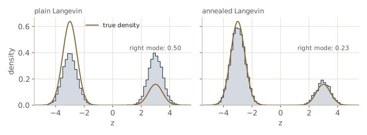
The third problem is the subject of Exercise 20.18 of Bishop & Bishop: if \(p = \lambda p_A + (1 - \lambda)p_B\) with components that do not overlap, then in the region of \(p_A\) the score is \(\nabla \ln (\lambda p_A) = \nabla \ln p_A\), and \(\lambda\) has dropped out. Langevin chains feel only the local shape; the fraction that ends up in each mode is decided by where the chains started. We demonstrate it with exact scores on a one-dimensional density with modes at \(\pm 3\) and weights 0.8 and 0.2, starting all chains from a broad symmetric distribution.
The remedy uses noise on purpose. Adding noise of a large variance smears the modes into each other, so that the score of the smoothed density does carry information about the weights, fills in low-density regions, and is defined everywhere; but it also distorts the density. So we use a sequence of noise levels \(\sigma_L > \dots > \sigma_1\), from large enough to connect everything to small enough to be faithful, and train one network \(\mathbf{s}(\mathbf{z}, \mathbf{w}, \sigma^2)\) with the noise level as an input and a weighted sum of denoising score matching losses, one per level. Sampling by annealed Langevin dynamics runs a few Langevin steps at each level, from \(\sigma_L\) down to \(\sigma_1\), handing the samples from one level to the next. The step size is scaled with the noise variance, since a smoother density tolerates longer steps.
def langevin(score, z, eta, n_steps):
    """Langevin dynamics: z <- z + eta * score(z) + sqrt(2 eta) * eps, for many chains at once."""
    for _ in range(n_steps):
        z = z + eta * score(z) + math.sqrt(2 * eta) * torch.randn_like(z)
    return z

w2, m2, s2 = torch.tensor([0.8, 0.2]), torch.tensor([-3.0, 3.0]), 0.5    # two well-separated modes

def score_two_modes(z, sigma):
    """Exact score of the two-mode density smoothed by Gaussian noise of standard deviation sigma."""
    var = s2 ** 2 + sigma ** 2
    r = torch.softmax(torch.log(w2) - (z[:, None] - m2) ** 2 / (2 * var), 1)
    return (r * (m2 - z[:, None])).sum(1) / var

torch.manual_seed(11)
z0 = 4.0 * torch.randn(10_000)                                    # broad, symmetric starting points
z_plain = langevin(lambda z: score_two_modes(z, 0.0), z0, eta=0.01, n_steps=1200)
z_ann = z0.clone()
for sig in torch.logspace(math.log10(4.0), math.log10(0.02), 12).tolist():   # sigma_L = 4 down to 0.02
    z_ann = langevin(lambda z: score_two_modes(z, sig), z_ann,
                     eta=0.04 * (s2 ** 2 + sig ** 2), n_steps=100)
print(f"weight of the right-hand mode: true 0.200   plain Langevin {(z_plain > 0).float().mean():.3f}   "
      f"annealed Langevin {(z_ann > 0).float().mean():.3f}")
print(f"spread within the left mode:   true {s2:.3f}   plain Langevin {z_plain[z_plain < 0].std():.3f}   "
      f"annealed Langevin {z_ann[z_ann < 0].std():.3f}")
weight of the right-hand mode: true 0.200   plain Langevin 0.496   annealed Langevin 0.230
spread within the left mode:   true 0.500   plain Langevin 0.511   annealed Langevin 0.508
Both samplers get the shape of each mode right, but plain Langevin puts about half the chains in the small mode, because about half of them started on its side. Annealing recovers the weights, 0.23 against the true 0.20 (figure 4).
This training procedure, a single network over many noise levels with a weighted sum of losses, is the diffusion model’s training procedure, and annealed Langevin sampling is the counterpart of the reverse chain. Our noise-prediction network already is a multi-level score model, so we can sample from it by annealed Langevin as well: twenty levels spaced along the chain, ten steps each, with \(\eta = 0.3(1 - \alpha_t)\), and at the end one jump to the estimate of the clean point, \((\mathbf{z}_t + (1 - \alpha_t)\,\mathbf{s})/\sqrt{\alpha_t}\) (Tweedie’s formula again).
@torch.no_grad()
def annealed_langevin(score_fn, n, levels, n_inner, c):
    """A few Langevin steps at each noise level, noisiest first, then one denoising jump."""
    z = torch.randn(n, 2)
    for t in levels:
        eta = c * (1 - alpha[t].item())
        for _ in range(n_inner):
            z = z + eta * score_fn(z, t) + math.sqrt(2 * eta) * torch.randn_like(z)
    a = alpha[levels[-1]].item()
    return (z + (1 - a) * score_fn(z, levels[-1])) / math.sqrt(a)

levels = list(range(T, 9, -10))                                 # t = 200, 190, ..., 10
torch.manual_seed(12)
report("annealed Langevin, network", annealed_langevin(net_score(g_net), 2000, levels, 10, 0.3), 200)
torch.manual_seed(12)
report("annealed Langevin, exact", annealed_langevin(lambda z, t: mixture_stats(z, alpha[t])[1],
                                                     2000, levels, 10, 0.3), 200)
annealed Langevin, network    200   mean ln p(x)  -1.679   energy distance 0.0039   classes [0.397 0.358 0.245]
annealed Langevin, exact      200   mean ln p(x)  -1.035   energy distance 0.0037   classes [0.3875 0.3645 0.248 ]
With the same 200 network evaluations, annealed Langevin gets the class weights right and a higher average log density than ancestral sampling, but a larger energy distance. The row with the exact score shows what is going on, and why we report two numbers: its average log density is higher than that of real data, because the final denoising jump pulls points onto the arms’ center lines (it outputs a posterior mean, not a sample), so the samples are too concentrated. The energy distance catches the lost spread.
Stochastic differential equations
Diffusion models work best with many small steps, so it is natural to take the limit of infinitely many (Song et al., 2020), much as module 18 took the limit of infinitely many residual layers to get neural ODEs. Let \(\tau = t/T \in [0, 1]\) be a continuous time and let the step variances shrink with the step size \(\Delta\tau = 1/T\), as \(\beta_t = \beta(\tau)\,\Delta\tau\) for a smooth rate \(\beta(\tau)\). Expanding \(\sqrt{1 - \beta(\tau)\Delta\tau} \approx 1 - \tfrac12\beta(\tau)\Delta\tau\), the noising step becomes
\[\mathbf{z}(\tau + \Delta\tau) - \mathbf{z}(\tau) \approx -\tfrac12 \beta(\tau)\,\mathbf{z}(\tau)\,\Delta\tau + \sqrt{\beta(\tau)\,\Delta\tau}\;\boldsymbol{\epsilon},\]and in the limit a stochastic differential equation (SDE),
\[d\mathbf{z} = \underbrace{-\tfrac12 \beta(\tau)\,\mathbf{z}\; d\tau}_{\text{drift}} + \underbrace{\sqrt{\beta(\tau)}\; d\mathbf{v}}_{\text{diffusion}} .\]The general form is \(d\mathbf{z} = \mathbf{f}(\mathbf{z}, \tau)\,d\tau + g(\tau)\,d\mathbf{v}\). The drift \(\mathbf{f}\) is a deterministic velocity, as in an ODE; the diffusion term adds Gaussian increments \(d\mathbf{v}\) whose variance equals the time step, which is why the noise enters with a square root of \(\Delta\tau\). Two remarkable facts make this view useful (Song et al., 2020, building on older results on time-reversed diffusions). First, the process can be run backward in time by another SDE,
\[d\mathbf{z} = \left[\mathbf{f}(\mathbf{z}, \tau) - g(\tau)^2\, \nabla_{\mathbf{z}} \ln q_\tau(\mathbf{z})\right] d\tau + g(\tau)\, d\mathbf{v},\]integrated from \(\tau = 1\) down to \(\tau = 0\), where \(q_\tau\) is the noisy marginal at time \(\tau\). The only unknown is the score of the noisy marginal, which is what our network estimates. Its simplest discretization with fixed steps, the Euler–Maruyama method, gives (with our \(\mathbf{f}\) and \(g\) and a step back of size \(\Delta\tau\)) \(\mathbf{z} \leftarrow \mathbf{z} + [\tfrac12\beta\mathbf{z} + \beta\,\mathbf{s}]\Delta\tau + \sqrt{\beta\Delta\tau}\,\boldsymbol{\epsilon}\), which agrees to first order in \(\beta_t\) with the ancestral step: \(\boldsymbol{\mu} = (\mathbf{z}_t + \beta_t\mathbf{s})/\sqrt{1 - \beta_t} \approx \mathbf{z}_t + \tfrac12\beta_t\mathbf{z}_t + \beta_t\mathbf{s}\). The same update also splits into two familiar pieces: a Langevin step on the score with step size \(\eta = \tfrac12\beta_t\), which contributes \(\tfrac12\beta_t\mathbf{s} + \sqrt{\beta_t}\,\boldsymbol{\epsilon}\), and a deterministic move \(\tfrac12\beta_t(\mathbf{z} + \mathbf{s})\), which we are about to meet again. Second, there is a deterministic process with the same marginals \(q_\tau\) at every time, the probability-flow ODE,
\[\frac{d\mathbf{z}}{d\tau} = \mathbf{f}(\mathbf{z}, \tau) - \tfrac12\, g(\tau)^2\, \nabla_{\mathbf{z}} \ln q_\tau(\mathbf{z}) = -\tfrac12\beta(\tau)\left[\mathbf{z} + \nabla_{\mathbf{z}} \ln q_\tau(\mathbf{z})\right].\]Run backward from \(\mathbf{z}(1) \sim \mathcal{N}(\mathbf{0}, \mathbf{I})\), it maps noise to data with no randomness after the first draw. Any ODE solver can be used, including adaptive ones that take large steps where the flow is smooth. And since the map from \(\mathbf{z}(1)\) to \(\mathbf{z}(0)\) is an invertible flow, the continuous change-of-variables formula of module 18 gives exact log likelihoods.
To use our discrete network in continuous time, we need \(\alpha(\tau)\) and \(\beta(\tau)\) consistent with the discrete schedule. We interpolate \(\ln\alpha\) linearly between the grid points \(\tau = t/T\), which makes \(\beta(\tau) = -d\ln\alpha/d\tau\) constant on each step interval and equal to \(-T\ln(1 - \beta_t) \approx T\beta_t\) there; the network is simply evaluated at the non-integer step \(\tau T\). Near \(\tau = 0\) the score blows up (the noise variance \(1 - \alpha(\tau)\) vanishes), so both samplers stop at \(\tau = 1/T\) and finish with one jump to the estimate of the clean point.
log_alpha = torch.log(alpha)                     # ln alpha_t for t = 0, ..., T (alpha_0 = 1)

def alpha_cont(tau):
    """alpha(tau) for tau in [0, 1]: ln alpha interpolated linearly between the grid points t / T."""
    s = tau * T
    i = min(int(s), T - 1)
    return math.exp(log_alpha[i] + (s - i) * (log_alpha[i + 1] - log_alpha[i]))

def beta_cont(tau):
    """beta(tau) = -d ln alpha / d tau, constant on each step interval ((t - 1)/T, t/T]."""
    i = min(max(math.ceil(tau * T - 1e-9), 1), T)
    return -T * (log_alpha[i] - log_alpha[i - 1]).item()

def net_g(net, c=None):
    """The noise network as a function of continuous time tau (it sees the step tau * T)."""
    def fn(z, tau):
        tt = torch.full((len(z),), tau * T)
        return net(z, tt) if c is None else net(z, tt, torch.full((len(z),), c))
    return fn

def pf_drift(g_fn, z, tau):
    """Right-hand side of the probability-flow ODE: -beta(tau)/2 * (z + score)."""
    score = -g_fn(z, tau) / math.sqrt(1 - alpha_cont(tau))
    return -0.5 * beta_cont(tau) * (z + score)

def denoise(g_fn, z, tau):
    """Final jump to the estimate of the clean point, (z - sqrt(1 - a) g) / sqrt(a)."""
    a = alpha_cont(tau)
    return (z - math.sqrt(1 - a) * g_fn(z, tau)) / math.sqrt(a)

@torch.no_grad()
def sample_ode(g_fn, z, n_steps, method="heun"):
    """Integrate the probability-flow ODE from tau = 1 down to tau = 1/T, then denoise."""
    taus = torch.linspace(1.0, 1.0 / T, n_steps + 1).tolist()
    for t0, t1 in zip(taus[:-1], taus[1:]):
        h = t1 - t0                                              # negative: time runs backward
        f0 = pf_drift(g_fn, z, t0)
        if method == "euler":
            z = z + h * f0
        else:                                                    # Heun: average the slopes at both ends
            z = z + 0.5 * h * (f0 + pf_drift(g_fn, z + h * f0, t1))
    return denoise(g_fn, z, 1.0 / T)

@torch.no_grad()
def sample_reverse_sde(g_fn, z, n_steps):
    """Euler-Maruyama steps on the reverse SDE from tau = 1 down to tau = 1/T, then denoise."""
    taus = torch.linspace(1.0, 1.0 / T, n_steps + 1).tolist()
    for t0, t1 in zip(taus[:-1], taus[1:]):
        dt, b = t0 - t1, beta_cont(t0)
        score = -g_fn(z, t0) / math.sqrt(1 - alpha_cont(t0))
        z = z + (0.5 * b * z + b * score) * dt + math.sqrt(b * dt) * torch.randn_like(z)
    return denoise(g_fn, z, 1.0 / T)

print(f"alpha(50/T) = {alpha_cont(50 / T):.6f}   alpha_50 = {alpha[50]:.6f}")
print(f"beta(50/T) / T = {beta_cont(50 / T) / T:.6f}   beta_50 = {beta[50]:.6f}")
alpha(50/T) = 0.686868   alpha_50 = 0.686868
beta(50/T) / T = 0.014961   beta_50 = 0.014849
Now we compare samplers that all use the same trained network, counting cost in network function evaluations (NFE). Heun’s method costs two evaluations per step, the other methods one; the final denoising jump adds one more.
g_fn = net_g(g_net)
torch.manual_seed(13)
z_T = torch.randn(2000, 2)                    # shared starting noise for the SDE and ODE samplers
torch.manual_seed(14)
report("ancestral (Algorithm 20.2)", sample_ddpm(net_eps(g_net), 2000)[0], T)
for n in [200, 20, 10]:
    torch.manual_seed(14)
    report(f"reverse SDE, {n} steps", sample_reverse_sde(g_fn, z_T, n), n + 1)
for n in [20, 10]:
    report(f"PF ODE Euler, {n} steps", sample_ode(g_fn, z_T, n, "euler"), n + 1)
for n in [100, 10]:
    report(f"PF ODE Heun, {n} steps", sample_ode(g_fn, z_T, n), 2 * n + 1)
x_ode = sample_ode(g_fn, z_T, 10, "euler")
rerun_gap = (x_ode - sample_ode(g_fn, z_T, 10, "euler")).abs().max()
print(f"ODE run twice from the same z_T: largest difference {rerun_gap:.1e}")
ancestral (Algorithm 20.2)    200   mean ln p(x)  -1.814   energy distance 0.0015   classes [0.418  0.3305 0.2515]
reverse SDE, 200 steps        201   mean ln p(x)  -1.815   energy distance 0.0015   classes [0.417  0.3305 0.2525]
reverse SDE, 20 steps          21   mean ln p(x)  -3.165   energy distance 0.0059   classes [0.3935 0.365  0.2415]
reverse SDE, 10 steps          11   mean ln p(x)  -5.810   energy distance 0.0101   classes [0.364 0.351 0.285]
PF ODE Euler, 20 steps         21   mean ln p(x)  -2.084   energy distance 0.0013   classes [0.3985 0.343  0.2585]
PF ODE Euler, 10 steps         11   mean ln p(x)  -2.469   energy distance 0.0016   classes [0.3955 0.343  0.2615]
PF ODE Heun, 100 steps        201   mean ln p(x)  -1.944   energy distance 0.0013   classes [0.3995 0.342  0.2585]
PF ODE Heun, 10 steps          21   mean ln p(x)  -2.467   energy distance 0.0015   classes [0.399 0.341 0.26 ]
ODE run twice from the same z_T: largest difference 0.0e+00
With 200 or so evaluations all the samplers are comparable. The difference shows at low cost. With 11 or 21 evaluations the reverse SDE falls apart, because a large stochastic step injects noise that the few remaining steps cannot remove, while the ODE, whose trajectories are smooth, still gives reasonable samples. On this problem plain Euler steps do as well as or better than Heun’s at equal cost; on images, higher-order and adaptive solvers are often worth their extra evaluations. The last line confirms that the ODE sampler is deterministic: the randomness is all in \(\mathbf{z}_T\). Figure 5 contrasts the two kinds of trajectories.
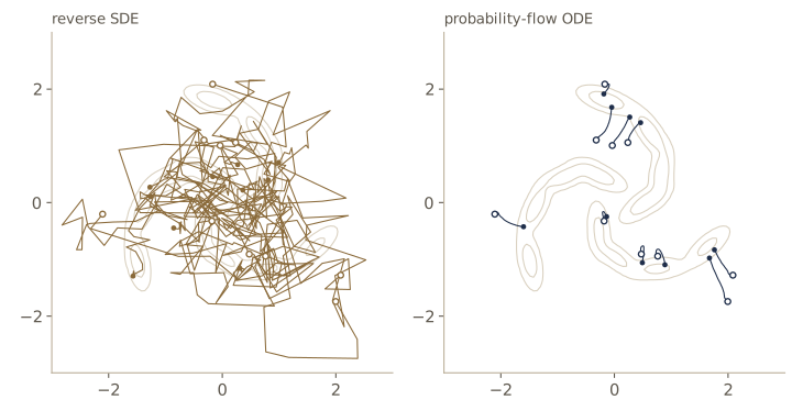
Finally, the likelihood. Along a trajectory of \(d\mathbf{z}/d\tau = \mathbf{f}(\mathbf{z}, \tau)\) the log density changes at the rate \(-\nabla \cdot \mathbf{f}\) (the instantaneous change of variables of module 18). Carrying a data point \(\mathbf{x}\) forward from \(\tau_0 = 1/T\) to \(\tau = 1\) and integrating,
\[\ln p_{\tau_0}(\mathbf{x}) = \ln \mathcal{N}\left(\mathbf{z}(1) \mid \mathbf{0}, \mathbf{I}\right) + \int_{\tau_0}^{1} \nabla \cdot \mathbf{f}\left(\mathbf{z}(\tau), \tau\right) d\tau .\]In two dimensions the divergence is cheap: two backward passes give the diagonal of the Jacobian exactly. (In high dimensions one uses a stochastic trace estimator instead, as for continuous flows.) We integrate the augmented system with Heun steps, first with the exact score, to validate the machinery against the true density \(q_{\tau_0}\), and then with the network. The ODE model is a different model from the discrete chain of the previous section, although both use the same network, so its likelihood and the chain’s ELBO measure different things; we print both for comparison.
def ode_log_likelihood(g_fn, x, n_steps=100):
    """ln p(x) under the flow defined by the probability-flow ODE, by carrying x from tau = 1/T to 1
    and accumulating the integral of div f (Heun steps), plus ln N(z(1) | 0, I)."""
    def drift_and_div(z, tau):
        z = z.detach().requires_grad_(True)
        f = pf_drift(g_fn, z, tau)
        div = sum(torch.autograd.grad(f[:, i].sum(), z, retain_graph=True)[0][:, i] for i in range(2))
        return f.detach(), div.detach()
    taus = torch.linspace(1.0 / T, 1.0, n_steps + 1).tolist()
    z, delta = x.clone(), torch.zeros(len(x))
    for t0, t1 in zip(taus[:-1], taus[1:]):
        h = t1 - t0
        f0, d0 = drift_and_div(z, t0)
        f1, d1 = drift_and_div(z + h * f0, t1)
        z, delta = z + 0.5 * h * (f0 + f1), delta + 0.5 * h * (d0 + d1)
    return -0.5 * (z ** 2).sum(1) - math.log(2 * math.pi) + delta

def exact_g(z, tau):
    """The ideal noise predictor at continuous time tau."""
    a = alpha_cont(tau)
    return -math.sqrt(1 - a) * mixture_stats(z, a)[1]

x_ll = X_test[:500]
print(f"true ln q(x) at tau = 1/T, averaged     {mixture_stats(x_ll, alpha[1])[0].mean():.3f}")
print(f"ODE likelihood with the exact score     {ode_log_likelihood(exact_g, x_ll).mean():.3f}")
print(f"ODE likelihood with the trained network {ode_log_likelihood(g_fn, x_ll).mean():.3f}")
torch.manual_seed(6)
print(f"ELBO of the discrete chain, same points {elbo(net_eps(g_net), x_ll).mean():.3f}")
true ln q(x) at tau = 1/T, averaged     -1.258
ODE likelihood with the exact score     -1.271
ODE likelihood with the trained network -1.411
ELBO of the discrete chain, same points -1.500
With the exact score, the ODE reproduces the true log density to about a hundredth of a nat, which validates the construction (the remaining gap comes from the time steps and from \(\mathbf{z}(1)\) not being exactly standard normal). With the trained network the model’s log likelihood is about 0.15 nats per point below the truth, and above the ELBO of the discrete chain. Exact likelihoods are one of the things the ODE view adds; they make diffusion models comparable with flows on the same footing.
Guided diffusion
So far the model generates from \(p(\mathbf{x})\). Most applications want \(p(\mathbf{x} \mid \mathbf{c})\), where the condition \(\mathbf{c}\) is a class label, a sentence, a low-resolution image, or an image with a hole in it. The direct approach feeds \(\mathbf{c}\) to the network as an extra input, \(\mathbf{g}(\mathbf{z}, \mathbf{w}, t, \mathbf{c})\), and trains on pairs \((\mathbf{x}_n, \mathbf{c}_n)\). It works, but the network is free to pay little attention to \(\mathbf{c}\), and we have no knob to trade how closely samples match the condition against how varied they are. Guidance adds that knob. Throughout this section, all scores are scores of noisy distributions at the current step, and our label is the arm \(c \in \{0, 1, 2\}\).
Classifier guidance
Suppose we have a classifier \(p(c \mid \mathbf{z}_t)\). Bayes’ theorem and the fact that \(p(c)\) does not depend on \(\mathbf{z}_t\) give
\[\nabla \ln p(\mathbf{z}_t \mid c) = \nabla \ln p(\mathbf{z}_t) + \nabla \ln p(c \mid \mathbf{z}_t) .\]The conditional score is the unconditional one plus the gradient of the classifier’s log probability, a push toward regions the classifier assigns to class \(c\) (Dhariwal and Nichol, 2021). Scaling the push by a guidance scale \(\lambda\) gives
\[\text{score}(\mathbf{z}_t, c, \lambda) = \nabla \ln p(\mathbf{z}_t) + \lambda\, \nabla \ln p(c \mid \mathbf{z}_t).\]With \(\lambda = 0\) we recover the unconditional model, with \(\lambda = 1\) the conditional one, and with \(\lambda > 1\) the samples are pushed toward points the classifier is sure about. In terms of the noise prediction, since \(\mathbf{s} = -\mathbf{g}/\sqrt{1 - \alpha_t}\), the guided prediction is \(\mathbf{g} - \lambda\sqrt{1 - \alpha_t}\,\nabla \ln p(c \mid \mathbf{z}_t)\), and the sampler is unchanged.
The classifier has to work on noisy inputs at every step, so it cannot be an ordinary classifier trained on clean data; it is trained on \((\mathbf{z}_t, t)\) pairs made with the diffusion kernel, and takes the step as an input. For our data we can compare its accuracy with the Bayes-optimal accuracy computed from the exact noisy class posterior.
class NoisyClassifier(nn.Module):
    """p(c | z_t, t): an MLP on the noisy point and the step embedding, returning class logits."""
    def __init__(self, hidden=64):
        super().__init__()
        self.net = nn.Sequential(nn.Linear(2 + 16, hidden), nn.SiLU(),
                                 nn.Linear(hidden, hidden), nn.SiLU(), nn.Linear(hidden, C))

    def forward(self, z, t):
        return self.net(torch.cat([z, time_embed(t)], 1))

torch.manual_seed(16)
clf = NoisyClassifier()
opt = torch.optim.Adam(clf.parameters(), lr=3e-3, foreach=True)
for step in range(1500):
    idx = torch.randint(0, N, (512,))
    t = torch.randint(1, T + 1, (512,))
    z_t = diffuse(X[idx], t[:, None], torch.randn(512, 2)).float()
    loss = F.cross_entropy(clf(z_t, t), labels[idx])
    opt.zero_grad()
    loss.backward()
    opt.step()
with torch.no_grad():
    for t in [10, 50, 100, 150]:
        z_t = diffuse(X_test, t, torch.randn(len(X_test), 2)).float()
        acc = (clf(z_t, torch.full((len(z_t),), t)).argmax(1) == labels_test).float().mean()
        bayes = (class_posterior(z_t, alpha[t]).argmax(1) == labels_test).float().mean()
        print(f"t = {t:3d}: classifier accuracy {acc:.3f}   Bayes-optimal accuracy {bayes:.3f}")
t =  10: classifier accuracy 0.989   Bayes-optimal accuracy 0.994
t =  50: classifier accuracy 0.735   Bayes-optimal accuracy 0.736
t = 100: classifier accuracy 0.533   Bayes-optimal accuracy 0.526
t = 150: classifier accuracy 0.431   Bayes-optimal accuracy 0.426
The classifier is as good as it can be at every noise level; as the noise grows, the label becomes impossible to read off and the accuracy falls toward the largest class weight.
Classifier-free guidance
Classifier guidance needs a second network trained on noisy data, and its gradient can be a poor guide: a classifier only has to find some feature that separates the classes and may ignore everything else about \(\mathbf{x}\). Classifier-free guidance (Ho and Salimans, 2022) removes the classifier. Substituting \(\nabla \ln p(c \mid \mathbf{z}_t) = \nabla \ln p(\mathbf{z}_t \mid c) - \nabla \ln p(\mathbf{z}_t)\) into the guided score gives
\[\text{score}(\mathbf{z}_t, c, \lambda) = \lambda\, \nabla \ln p(\mathbf{z}_t \mid c) + (1 - \lambda)\, \nabla \ln p(\mathbf{z}_t),\]a combination of a conditional and an unconditional score. For \(0 < \lambda < 1\) it interpolates between them; for \(\lambda > 1\) the unconditional score enters with a negative sign, pushing samples away from what an unconditional model would produce and toward what distinguishes class \(c\). Both scores come from one network: during training, the label is replaced by a special null value with some probability (we use 15%), so the network learns \(\mathbf{g}(\mathbf{z}, \mathbf{w}, t, c)\) and \(\mathbf{g}(\mathbf{z}, \mathbf{w}, t, \varnothing)\) at once. This is like dropout (module 09) applied to the whole conditioning input. In noise form the guided prediction is \(\lambda\,\mathbf{g}(\mathbf{z}_t, \mathbf{w}, t, c) + (1 - \lambda)\,\mathbf{g}(\mathbf{z}_t, \mathbf{w}, t, \varnothing)\), at the cost of two network evaluations per step.
torch.manual_seed(15)
cfg_net = train_ddpm(NoiseNet(n_classes=C), X, labels=labels, p_drop=0.15)
step   500   loss (mean of last 500) 0.5335
step  1000   loss (mean of last 500) 0.4402
step  1500   loss (mean of last 500) 0.4269
step  2000   loss (mean of last 500) 0.4215
step  2500   loss (mean of last 500) 0.4171
step  3000   loss (mean of last 500) 0.4134
Now we sample class \(c = 2\), the smallest arm, at several guidance scales with both methods, and measure four things: the share of samples that the true class posterior assigns to class 2; the average \(\ln p(c \mid \mathbf{x})\) under the true posterior (how unambiguous the samples are); the energy distance to real class-2 test points; and how the samples that land on the arm spread over its four components, from the inner end of the arm to the outer end (real data put about a quarter in each). A fresh sample from the true class-2 distribution gives the reference row.
def classifier_guided_eps(net, clf, c, lam):
    """Noise prediction for the classifier-guided score: g - lam sqrt(1 - alpha_t) grad ln p(c | z_t)."""
    def fn(z, t):
        tt = torch.full((len(z),), t)
        with torch.enable_grad():
            zg = z.clone().requires_grad_(True)
            grad = torch.autograd.grad(F.log_softmax(clf(zg, tt), 1)[:, c].sum(), zg)[0]
        return net(z, tt) - lam * math.sqrt(1 - alpha[t].item()) * grad
    return fn

def cfg_eps(net, c, lam):
    """Noise prediction for classifier-free guidance: lam g(z, c) + (1 - lam) g(z, null)."""
    def fn(z, t):
        tt = torch.full((len(z),), t)
        g_cond = net(z, tt, torch.full((len(z),), c))
        g_null = net(z, tt, torch.full((len(z),), C))                   # label C = "no label"
        return lam * g_cond + (1 - lam) * g_null
    return fn

def guided_report(name, xs, c):
    post = class_posterior(xs, 1.0)
    on = post.argmax(1) == c
    resp = mixture_stats(xs[on], 1.0)[2][:, comp_class == c]             # this arm's four components
    spread = resp.argmax(1).bincount(minlength=J) / on.sum()
    print(f"{name:20s} on class {(post.argmax(1) == c).float().mean():6.1%}   "
          f"mean ln p(c|x) {post[:, c].clamp_min(1e-12).log().mean():7.3f}   "
          f"energy distance {energy_distance(xs, X_test[labels_test == c]):.4f}   "
          f"inner to outer {spread.numpy()}")

c = 2
x_ref, lab_ref = sample_mixture(4000, np.random.default_rng(17))
guided_report("true p(x | c)", x_ref[lab_ref == c][:1000], c)
for lam in [0.0, 1.0, 3.0, 8.0]:
    torch.manual_seed(17)
    x_guided = sample_ddpm(classifier_guided_eps(g_net, clf, c, lam), 1000)[0]
    guided_report(f"classifier, lam = {lam:.0f}", x_guided, c)
for lam in [0.0, 1.0, 3.0, 8.0]:
    torch.manual_seed(17)
    guided_report(f"free, lam = {lam:.0f}", sample_ddpm(cfg_eps(cfg_net, c, lam), 1000)[0], c)
true p(x | c)        on class  99.9%   mean ln p(c|x)  -0.006   energy distance 0.0009   inner to outer [0.237  0.262  0.2453 0.2557]
classifier, lam = 0  on class  23.6%   mean ln p(c|x) -18.389   energy distance 0.8925   inner to outer [0.2542 0.2034 0.2161 0.3263]
classifier, lam = 1  on class  93.5%   mean ln p(c|x)  -0.704   energy distance 0.0061   inner to outer [0.2257 0.2417 0.2299 0.3027]
classifier, lam = 3  on class  99.9%   mean ln p(c|x)  -0.007   energy distance 0.1696   inner to outer [0.0571 0.1602 0.3654 0.4174]
classifier, lam = 8  on class 100.0%   mean ln p(c|x)  -0.000   energy distance 0.4711   inner to outer [0.006 0.065 0.35  0.579]
free, lam = 0        on class  22.6%   mean ln p(c|x) -17.825   energy distance 0.9162   inner to outer [0.2345 0.2124 0.2566 0.2965]
free, lam = 1        on class  99.7%   mean ln p(c|x)  -0.030   energy distance 0.0028   inner to outer [0.2447 0.2538 0.2227 0.2788]
free, lam = 3        on class 100.0%   mean ln p(c|x)  -0.000   energy distance 0.2415   inner to outer [0.037 0.12  0.442 0.401]
free, lam = 8        on class 100.0%   mean ln p(c|x)  -0.000   energy distance 0.3177   inner to outer [0.011 0.028 0.767 0.194]
The pattern is the same for both methods. At \(\lambda = 0\) the label is ignored and only about a quarter of the samples land on the requested arm. At \(\lambda = 1\) most or nearly all do, the energy distance to the real class-2 data is smallest, and the samples cover the arm evenly, as the true conditional does. Pushing \(\lambda\) higher makes every sample unambiguously class 2, with \(\ln p(c \mid \mathbf{x})\) essentially zero, but the samples retreat from the inner end of the arm, where it comes close to the other arms, toward the outer half where no other class is near. The energy distance grows accordingly. That is the diversity–fidelity trade-off of guidance in miniature: large guidance scales give samples that are typical of the class in the classifier’s eyes, and less representative of the class as a whole. At \(\lambda = 1\) the classifier-free model is the more accurate of the two here, because its conditional branch learned the class-2 density directly rather than by combining an unconditional model with a separate classifier. Figure 6 shows the samples. Its bottom-left panel also shows a cost of label dropout: the unconditional branch of the classifier-free network saw only 15% of the training examples, and its samples are visibly more scattered off the arms than those of the dedicated unconditional network in the top-left panel.
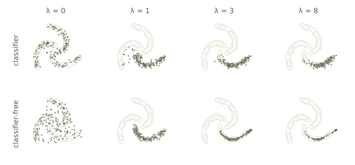
Watch out. For \(\lambda\) other than 0 and 1, it is tempting to think the guided sampler draws from the sharpened density proportional to \(p(\mathbf{x})\,p(c \mid \mathbf{x})^{\lambda}\). It does not, exactly: the guided field at step \(t\) is built from the noisy \(p(\mathbf{z}_t)\) and \(p(c \mid \mathbf{z}_t)\), and noising a sharpened density is not the same as sharpening the noisy one, so the field is in general not the score of the noised sharpened density. Guidance is best seen as a well-behaved heuristic whose effect we measure, as above, rather than derive.
The same machinery powers the applications that made diffusion models famous. In text-to-image models the condition is a prompt; a transformer language model (module 12) encodes it, and the denoising U-net reads the encoding through cross-attention layers, with classifier-free guidance sharpening the match between image and text. For super-resolution the condition is a low-resolution image and the model samples plausible high-resolution versions, several stages of which can be cascaded to reach large images. Inpainting, colorization, deblurring, and video generation follow the same pattern. To cut the cost of denoising in pixel space, latent diffusion (Rombach et al., 2022) first trains an autoencoder (module 19), then runs the whole diffusion model in its lower-dimensional latent space, and decodes the result with the autoencoder’s decoder. Bishop & Bishop §20.4 surveys these developments.
Looking back over the course
This module closes the course, and it is a good place to see how the pieces fit. After the overview of module 01, we started with probability and the standard distributions (modules 02–03) and with single-layer models for regression and classification (modules 04–05), where the network view of linear models first appeared. Deep networks (module 06), gradient descent (module 07), backpropagation (module 08), and regularization (module 09) gave us the machinery to train anything differentiable. Convolutional networks (module 10), transformers (module 12), and graph networks (module 13) built prior knowledge about images, sequences, and graphs into the architecture. Structured distributions and sampling (modules 11 and 14) and latent-variable models (modules 15 and 16) supplied the probabilistic toolkit, and the last four modules used all of it to build generative models: adversarial training (17), invertible flows (18), variational autoencoders (19), and now diffusion. A diffusion model on images uses almost everything at once: a U-net trained with Adam and backpropagation, an ELBO derived from a latent-variable model, a Markov chain, Langevin-style sampling, a transformer for the text prompt, and an ODE view that makes it a normalizing flow. The same few ideas, likelihoods and their bounds, gradients through computation graphs, and architectures that respect the structure of the data, keep recurring, and they are what we hope you carry beyond the course.
Summary
| Idea | What it does | Key equation or property |
|---|---|---|
| Forward encoder | fixed noising chain, data to \(\mathcal{N}(\mathbf{0}, \mathbf{I})\) | \(q(\mathbf{z}_t \mid \mathbf{z}_{t-1}) = \mathcal{N}(\sqrt{1 - \beta_t}\,\mathbf{z}_{t-1}, \beta_t\mathbf{I})\) |
| Diffusion kernel | sample any step in one draw | \(\mathbf{z}_t = \sqrt{\alpha_t}\,\mathbf{x} + \sqrt{1 - \alpha_t}\,\boldsymbol{\epsilon}_t\), \(\alpha_t = \prod_{\tau \le t}(1 - \beta_\tau)\) |
| Reverse conditional | tractable target for each reverse step | \(q(\mathbf{z}_{t-1} \mid \mathbf{z}_t, \mathbf{x}) = \mathcal{N}(\mathbf{m}_t, \sigma_t^2\mathbf{I})\), \(\sigma_t^2 = \beta_t(1 - \alpha_{t-1})/(1 - \alpha_t)\) |
| Reverse decoder | learned Gaussian steps | \(p(\mathbf{z}_{t-1} \mid \mathbf{z}_t, \mathbf{w}) = \mathcal{N}(\boldsymbol{\mu}(\mathbf{z}_t, \mathbf{w}, t), \beta_t\mathbf{I})\) |
| ELBO | training objective | reconstruction \(-\sum_t\) KL consistency terms, each a squared error |
| Noise prediction | simplified loss | \(\lVert \mathbf{g}(\sqrt{\alpha_t}\,\mathbf{x} + \sqrt{1 - \alpha_t}\,\boldsymbol{\epsilon}, \mathbf{w}, t) - \boldsymbol{\epsilon} \rVert^2\) |
| Score | noise predictor is a scaled score | \(\mathbf{s} = -\mathbf{g}/\sqrt{1 - \alpha_t}\); ideal \(\mathbf{g} = \mathbb{E}[\boldsymbol{\epsilon} \mid \mathbf{z}_t]\) |
| Denoising score matching | learn a score without knowing it | same minimizer as the explicit loss; differs by a constant |
| Annealed Langevin | sample from multi-level scores | Langevin steps from large to small noise |
| SDE and probability-flow ODE | continuous-time samplers, exact likelihood | \(d\mathbf{z}/d\tau = -\tfrac12\beta(\tau)[\mathbf{z} + \nabla\ln q_\tau(\mathbf{z})]\) |
| Classifier guidance | condition an unconditional model | \(\nabla\ln p(\mathbf{z}_t) + \lambda\nabla\ln p(c \mid \mathbf{z}_t)\) |
| Classifier-free guidance | one network with label dropout | \(\lambda\,\mathbf{g}(\mathbf{z}, c) + (1 - \lambda)\,\mathbf{g}(\mathbf{z}, \varnothing)\) |
Ideas to carry forward:
- A diffusion model trains one network on a simple regression problem, predicting the noise that was added, at every noise level. The ELBO, the simplified loss, and denoising score matching are three derivations of that same problem that differ only in how they weight the levels.
- The fixed Gaussian encoder is what makes everything tractable: the kernel \(q(\mathbf{z}_t \mid \mathbf{x})\) lets us sample any step directly, and \(q(\mathbf{z}_{t-1} \mid \mathbf{z}_t, \mathbf{x})\) gives a Gaussian target for every reverse step.
- Many noise levels are essential. Large noise connects the modes, fills in empty regions, and gets the mixture weights right; small noise restores detail.
- Sampling is where the cost is and where the choices are: ancestral steps, Langevin steps, SDE and ODE solvers, and guidance all reuse the same trained network.
Exercises
- Using the mean and covariance recursion for one noising step, show that if \(\beta_t = \beta\) is constant the covariance of \(\mathbf{z}_t\) approaches \(\mathbf{I}\) geometrically, with the deviation shrinking by the factor \(1 - \beta\) per step. Starting the chain from our whole training set, compute the empirical covariance of \(\mathbf{z}_t\) at several \(t\) with
forward_stepand compare with the recursion. - Show that \(\alpha_T \to 0\) as \(T \to \infty\) whenever \(\sum_t \beta_t\) diverges. For our schedule, compute \(\mathrm{KL}(q(\mathbf{z}_T \mid \mathbf{x}) \Vert \mathcal{N}(\mathbf{0}, \mathbf{I}))\) for the training point farthest from the origin. How large would \(\beta_T\) need to be, with the same linear shape and \(T = 50\), to keep it below 0.01 nats?
- Take the logarithm of Bayes’ theorem for \(q(\mathbf{z}_{t-1} \mid \mathbf{z}_t)\) and expand \(\ln q(\mathbf{z}_{t-1})\) to first order around \(\mathbf{z}_t\). Show that \(q(\mathbf{z}_{t-1} \mid \mathbf{z}_t)\) is approximately Gaussian with covariance \(\beta_t\mathbf{I}\) and find the leading correction to its mean. Check your formula for the mean with the one-dimensional grid code at \(\beta = 0.005\).
- Derive the Gaussian KL formula used in
kl_iso. Then modifyelboto use the reverse variance \(\sigma_t^2\) in place of \(\beta_t\) for \(t \ge 2\), keeping everything else. Which choice gives the higher bound for the ideal noise predictor and for the trained network? Explain the result using the form of the constant term. - Train the network on the true ELBO weights, \(\beta_t / \{2(1 - \alpha_t)(1 - \beta_t)\}\) per step, instead of the simplified loss. Compare the per-step losses, the ELBO, and the sample quality with the network in the notes. Then try sampling \(t\) non-uniformly with probability proportional to the weight, which leaves the expected loss unchanged, and compare the training curves.
- Instead of the noise, let the network predict the clean point \(\hat{\mathbf{x}}(\mathbf{z}_t, \mathbf{w}, t)\). Express \(\boldsymbol{\mu}\) in terms of \(\hat{\mathbf{x}}\), show that the consistency term becomes a weighted squared error \(\lVert \hat{\mathbf{x}} - \mathbf{x} \rVert^2\), and find the weight. Train this version with an unweighted loss and compare the samples with the noise-predicting network. Which steps does each parameterization emphasize?
- For a one-dimensional model, integrate by parts to show that \(J(w) = \int \{ s'(x, w) + \tfrac12 s(x, w)^2 \} p(x)\,dx + \text{const}\), which needs no knowledge of the true score (Hyvärinen’s score matching). Fit a linear score \(s(x) = ax + b\) to samples from a Gaussian by minimizing this loss and by minimizing denoising score matching with several values of \(\sigma\). Show that the denoising estimate of \(a\) is biased toward the smoothed variance and approaches the other as \(\sigma \to 0\).
- In the two-mode Langevin experiment, vary the number of noise levels (2, 4, 12) and the largest level \(\sigma_L\) (0.5, 1, 4). How large must \(\sigma_L\) be, relative to the separation of the modes, for annealing to recover the weights? Explain the answer using the score of the smoothed density at the midpoint between the modes.
- The DDIM update from step \(t\) to an earlier step \(s\) is \(\mathbf{z}_s = \sqrt{\alpha_s}\,\hat{\mathbf{x}} + \sqrt{1 - \alpha_s}\,\mathbf{g}(\mathbf{z}_t, \mathbf{w}, t)\), with \(\hat{\mathbf{x}} = (\mathbf{z}_t - \sqrt{1 - \alpha_t}\,\mathbf{g})/\sqrt{\alpha_t}\). Show that for \(s\) close to \(t\) it agrees to first order with an Euler step of the probability-flow ODE. Implement it with 10 and 20 steps and compare with the Euler ODE sampler at equal cost.
- Train a classifier on clean data only (\(t = 0\)) and use it for classifier guidance by evaluating it on \(\mathbf{z}_t\). What happens to the on-class rate and the energy distance at \(\lambda = 1\) and \(\lambda = 3\)? Explain the failure by looking at the classifier’s gradients at large \(t\).
- Repeat the guidance experiment for all three classes and plot, for each method, the on-class rate against the energy distance as \(\lambda\) runs from 0 to 8. Where on the curve would you operate if you wanted samples that a user would recognize as the requested class but that still looked varied?
- In your own words: how can a network trained only to guess the noise that was added to a data point generate completely new data? Explain it to a classmate who knows what an autoencoder is but has never seen a diffusion model, and say where the randomness of a new sample comes from.
Going further
- Bishop & Bishop, Deep Learning: Foundations and Concepts, chapter 20 — the source for this module. Exercises 20.1–20.5 (the forward process and its kernel), 20.6–20.7 (the reverse conditional), 20.8–20.13 (the ELBO and noise prediction), 20.14–20.18 (score matching), and 20.19–20.20 (SDEs and guidance) complement the ones above.
- Jonathan Ho, Ajay Jain, and Pieter Abbeel, “Denoising diffusion probabilistic models,” NeurIPS 2020, arXiv:2006.11239 — the noise-prediction parameterization and the simplified loss.
- Yang Song, Jascha Sohl-Dickstein, Diederik P. Kingma, Abhishek Kumar, Stefano Ermon, and Ben Poole, “Score-based generative modeling through stochastic differential equations,” ICLR 2021, arXiv:2011.13456 — the SDE view, the reverse SDE, and the probability-flow ODE.
- Jonathan Ho and Tim Salimans, “Classifier-free diffusion guidance,” arXiv:2207.12598 — guidance without a classifier.
- Calvin Luo, “Understanding diffusion models: a unified perspective,” arXiv:2208.11970 — a careful tutorial that derives the ELBO, score, and guidance views side by side.
- Related modules: Langevin sampling and energy-based models in module 14; the ELBO in module 15 and module 19, where the denoising autoencoder first met the score; continuous flows in module 18; U-nets in module 10; and variational inference in Intro to ML, module 10.
These notes follow the chapters of C. M. Bishop and H. Bishop, Deep Learning: Foundations and Concepts (Springer, 2024), the course text, which the authors make free to read online. The explanations, code, figures, and exercises here are written for this course; the book remains the reference, with the full derivations and many more exercises.