CSE 676 · Module 17 · Week 12
Generative Adversarial Networks
Adversarial training of a generator against a discriminator, the optimal discriminator and the Jensen–Shannon divergence, practical training (non-saturating loss, mode collapse, least-squares and Wasserstein variants), convolutional and conditional image GANs, and CycleGAN.
Companion reading: Bishop & Bishop, Deep Learning: Foundations and Concepts, chapter 17, “Generative Adversarial Networks”
By the end of this module you can
- Write down the GAN error function, explain why the generator ascends it while the discriminator descends it, and implement both losses stably from logits.
- Derive the optimal discriminator and show that, against it, the generator’s objective is a constant minus twice the Jensen–Shannon divergence, then check both results numerically.
- Train a small GAN on a two-dimensional mixture of Gaussians and measure mode coverage and sample quality during training.
- Explain why the original generator loss saturates when the discriminator is confident, derive the non-saturating loss, and measure the difference in gradient size and in training progress.
- Recognize mode collapse and the rotational dynamics of two-player games, and describe the least-squares, instance-noise, and Wasserstein remedies.
- Estimate a Wasserstein distance with a gradient-penalty critic and explain why it keeps a useful signal when the Jensen–Shannon divergence saturates.
- Build a small convolutional conditional GAN for digits and describe progressive growing, StyleGAN, and BigGAN at the level of ideas.
- Define the cycle-consistency loss of CycleGAN and show on two toy domains that it turns unpaired translation into a pair of mutually inverse maps.
Contents
Module 16 ended with a problem. A nonlinear latent-variable model, a simple distribution over a latent vector \(\mathbf{z}\) followed by a deep network that maps \(\mathbf{z}\) to data space, is easy to sample from and very expressive, but its likelihood is an integral over \(\mathbf{z}\) that we cannot compute. Modules 17 to 20 are four ways around that integral. This module takes the most radical one: give up on the likelihood altogether and train the network by a game.
A generative adversarial network (GAN) pairs the generator network with a second network, a classifier that tries to tell real training examples from the generator’s output. The classifier is trained to be right; the generator is trained to make it wrong. Nothing in this setup requires a density: the generator is judged only by the samples it produces. That freedom let GANs produce some of the first convincing high-resolution synthetic images, and it is also why they are harder to train and evaluate than the other three families.
We start with the loss function and derive what the game optimizes when both players are perfect: the Jensen–Shannon divergence between the data and the model. Then we train GANs on a two-dimensional mixture, where every failure mode is visible, and meet the fixes that practice relies on: the non-saturating generator loss, least-squares and Wasserstein objectives, and gradient penalties. The last part moves to images (convolutional and conditional GANs, trained on small MNIST digits) and to CycleGAN, which learns to translate between two domains without paired examples. Everything runs on a CPU in under two minutes; the text says where a GPU and more data would change the picture. We build on backpropagation (module 08), Adam (module 07), transposed convolutions (module 10), and the Kullback–Leibler divergence (module 02).
import math
import time
import numpy as np
import torch
import torch.nn as nn
import torch.nn.functional as F
from torchvision import datasets

np.set_printoptions(precision=4, suppress=True)
rng = np.random.default_rng(17)
torch.manual_seed(17)
Adversarial training
A generator without a likelihood
Start from the model of module 16. Draw a latent vector from a fixed, simple distribution,
\[p(\mathbf{z}) = \mathcal{N}(\mathbf{z} \mid \mathbf{0}, \mathbf{I}),\]and push it through a deep network \(\mathbf{x} = \mathbf{g}(\mathbf{z}, \mathbf{w})\) with parameters \(\mathbf{w}\), called the generator. Together, \(p(\mathbf{z})\) and \(\mathbf{g}\) define a distribution \(p_G(\mathbf{x})\) over data space: the distribution of \(\mathbf{g}(\mathbf{z}, \mathbf{w})\) when \(\mathbf{z}\) is random. We can sample from \(p_G\) with one forward pass, but we cannot evaluate \(p_G(\mathbf{x})\) at a given point. If the latent dimension \(M\) is smaller than the data dimension \(D\), all of the probability sits on an \(M\)-dimensional surface in data space and \(p_G\) has no ordinary density at all; even when \(M = D\), evaluating it would need the inverse of \(\mathbf{g}\) and the determinant of its Jacobian, which is exactly the constraint that normalizing flows (module 18) accept. A model that we can sample from but whose density we cannot evaluate is called an implicit generative model.
Without a likelihood we cannot fit \(\mathbf{w}\) by maximum likelihood. The idea of GANs is to learn a measure of how well the samples match the data at the same time as the generator. A second network \(d(\mathbf{x}, \boldsymbol{\phi})\), the discriminator, receives a data vector and outputs the probability that it came from the training set rather than from the generator. The discriminator is an ordinary binary classifier, and training it is supervised learning with labels we get for free: real examples are one class, generated examples the other. The generator is then trained to push the discriminator’s output on its samples toward “real”. Figure 1 shows the arrangement.
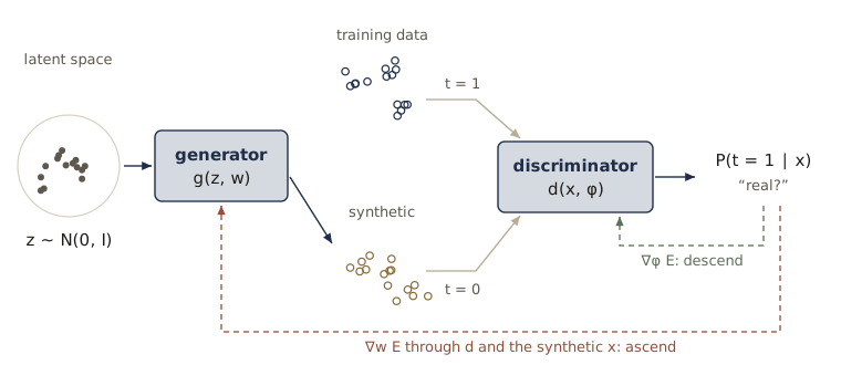
Our running example is a distribution whose structure we know exactly: an equal-weight mixture of six Gaussians of standard deviation 0.1, with centers on a regular hexagon of radius 2. Each mixture component is a mode, and a good generator must put samples near all six. The generator maps an 8-dimensional latent vector to the plane; both networks are small multilayer perceptrons. The discriminator network outputs a single logit \(a(\mathbf{x}, \boldsymbol{\phi})\), and \(d = \sigma(a)\) is applied inside the loss, as usual for binary classifiers.
K = 6                                                    # modes of the data distribution
angles = torch.arange(K) * (2 * math.pi / K)
MU = 2.0 * torch.stack([torch.cos(angles), torch.sin(angles)], dim=1)   # (K, 2) centers
SIG = 0.1

def sample_data(n, gen):
    """n points from the equal-weight mixture of K Gaussians on a hexagon."""
    k = torch.randint(0, K, (n,), generator=gen)
    return MU[k] + SIG * torch.randn(n, 2, generator=gen)

def mlp(d_in, d_out, width=64):
    return nn.Sequential(nn.Linear(d_in, width), nn.LeakyReLU(0.2),
                         nn.Linear(width, width), nn.LeakyReLU(0.2),
                         nn.Linear(width, d_out))

def n_params(net):
    return sum(p.numel() for p in net.parameters())

M = 8                                                    # latent dimension
g_net, d_net = mlp(M, 2), mlp(2, 1)                      # g(z, w) and the logit a(x, phi)
print("generator parameters", n_params(g_net), "  discriminator parameters", n_params(d_net))
generator parameters 4866 discriminator parameters 4417
To follow training we need a way to score a set of samples against the known mixture. Assign each sample to its nearest center and call it good if it lies within three standard deviations (0.3) of that center; a mode counts as covered if it receives at least 2% of the samples (a perfect generator gives each mode about 17%). The fraction of good samples measures quality, the number of covered modes measures diversity, and a generator can do well on one while failing the other.
def coverage(x):
    """(number of modes covered, fraction of good samples) for samples x of shape (n, 2)."""
    dist = torch.cdist(x, MU)                            # (n, K) distances to the centers
    d_min, k = dist.min(dim=1)
    good = d_min < 3 * SIG
    counts = torch.bincount(k[good], minlength=K)
    return int((counts >= 0.02 * len(x)).sum()), good.float().mean().item()

gen = torch.Generator().manual_seed(0)
modes, quality = coverage(sample_data(2000, gen))
print(f"real data:           modes covered {modes}   good fraction {quality:.3f}")
with torch.no_grad():
    modes, quality = coverage(g_net(torch.randn(2000, M, generator=gen)))
print(f"untrained generator: modes covered {modes}   good fraction {quality:.3f}")
real data:           modes covered 6   good fraction 0.988
untrained generator: modes covered 0   good fraction 0.000
Even real data scores slightly below 1, because a two-dimensional Gaussian puts about 1% of its mass beyond three standard deviations. The untrained generator puts its samples in a small blob near the origin, far from every mode.
The loss function
Label real examples with \(t = 1\) and generated ones with \(t = 0\). The discriminator’s output is its estimate of \(P(t = 1 \mid \mathbf{x})\), and we train it with the cross-entropy error of module 05,
\[E(\mathbf{w}, \boldsymbol{\phi}) = -\frac{1}{N}\sum_{n=1}^{N}\left\{t_n \ln d_n + (1 - t_n)\ln(1 - d_n)\right\},\]with \(d_n = d(\mathbf{x}_n, \boldsymbol{\phi})\). The training set of the discriminator consists of real points \(\mathbf{x}_n\) and synthetic points \(\mathbf{g}(\mathbf{z}_n, \mathbf{w})\) with fresh \(\mathbf{z}_n \sim p(\mathbf{z})\). Splitting the sum by label and averaging each part over its own examples (we use equally many of each, so this is the same error up to a factor of 2), the GAN error function is
\[E_{\mathrm{GAN}}(\mathbf{w}, \boldsymbol{\phi}) = -\frac{1}{N_{\mathrm{real}}}\sum_{n \in \mathrm{real}} \ln d(\mathbf{x}_n, \boldsymbol{\phi}) - \frac{1}{N_{\mathrm{synth}}}\sum_{n \in \mathrm{synth}} \ln\bigl(1 - d(\mathbf{g}(\mathbf{z}_n, \mathbf{w}), \boldsymbol{\phi})\bigr).\]The two networks want opposite things from this one number. The discriminator wants it small (classify correctly); the generator wants it large (make the discriminator fail on synthetic points). Training is the minimax problem
\[\min_{\boldsymbol{\phi}} \; \max_{\mathbf{w}} \; E_{\mathrm{GAN}}(\mathbf{w}, \boldsymbol{\phi}),\]and with stochastic gradients on mini-batches the updates are gradient descent for one player and gradient ascent for the other, with learning rate \(\eta\):
\[\Delta\boldsymbol{\phi} = -\eta\, \nabla_{\boldsymbol{\phi}} E_{\mathrm{GAN}}, \qquad \Delta\mathbf{w} = +\eta\, \nabla_{\mathbf{w}} E_{\mathrm{GAN}}.\]Only the second term of \(E_{\mathrm{GAN}}\) depends on \(\mathbf{w}\), and its gradient reaches the generator through the discriminator: by the chain rule, \(\nabla_{\mathbf{w}}\) of \(\ln(1 - d(\mathbf{g}(\mathbf{z}, \mathbf{w})))\) is the derivative of the log with respect to \(d\), times the gradient of \(d\) with respect to its input \(\mathbf{x}\), times the Jacobian of \(\mathbf{g}\) with respect to \(\mathbf{w}\). So the generator learns in which direction to move each sample to look more real, and backpropagation in one graph that contains both networks computes it. In practice the two players take turns: one mini-batch step for the discriminator, then one for the generator with a fresh batch of samples, and repeat.
Definition. A two-player zero-sum game is a pair of players whose payoffs add to zero: whatever one gains, the other loses. Here the payoff is \(E_{\mathrm{GAN}}\) for the generator and \(-E_{\mathrm{GAN}}\) for the discriminator. A solution is a Nash equilibrium, a pair \((\mathbf{w}^\star, \boldsymbol{\phi}^\star)\) at which neither player can improve by changing only its own parameters. It is a saddle point of \(E_{\mathrm{GAN}}\), not a minimum, which is why ordinary intuition about gradient descent does not carry over.
In code we never form \(d = \sigma(a)\) and then take its log: as soon as the discriminator is confident, \(\sigma(a)\) rounds to 0 or 1 in floating point and the log becomes infinite. The identities \(\ln\sigma(a) = -\operatorname{softplus}(-a)\) and \(\ln(1 - \sigma(a)) = -\operatorname{softplus}(a)\), with \(\operatorname{softplus}(a) = \ln(1 + e^{a})\), give a stable version. The generator’s part of the error comes in two versions that the next sections compare; we write both now. Minimizing g_error_saturating is the same as maximizing \(E_{\mathrm{GAN}}\) over \(\mathbf{w}\).
def d_error(a_real, a_fake):
    """E_GAN from logits: -mean ln d(x) - mean ln(1 - d(g(z)))."""
    return F.softplus(-a_real).mean() + F.softplus(a_fake).mean()

def g_error_saturating(a_fake):
    """The generator's part of E_GAN with the sign flipped: minimize mean ln(1 - d(g(z)))."""
    return -F.softplus(a_fake).mean()

def g_error_nonsaturating(a_fake):
    """The alternative generator loss: minimize -mean ln d(g(z))."""
    return F.softplus(-a_fake).mean()

a_real, a_fake = torch.randn(5), torch.randn(5)
d_r, d_f = torch.sigmoid(a_real), torch.sigmoid(a_fake)
direct = -(torch.log(d_r).mean() + torch.log(1 - d_f).mean())
library = (F.binary_cross_entropy_with_logits(a_real, torch.ones(5))
           + F.binary_cross_entropy_with_logits(a_fake, torch.zeros(5)))
print("matches the direct formula:", torch.allclose(d_error(a_real, a_fake), direct),
      "  matches PyTorch's BCE:", torch.allclose(d_error(a_real, a_fake), library))
a_big = torch.tensor([-120.0])                            # a very confident discriminator
print(f"direct formula at a = -120: {-torch.log(torch.sigmoid(a_big)).item()}"
      f"   stable version: {g_error_nonsaturating(a_big).item():.1f}")
matches the direct formula: True   matches PyTorch's BCE: True
direct formula at a = -120: inf   stable version: 120.0
The optimal discriminator
What does this game converge to when both networks are flexible enough to represent anything? To answer, replace the averages by expectations (the limit of infinitely many samples) and write the generator’s contribution as an expectation over \(p_G\):
\[E(p_G, d) = -\int p_{\mathrm{data}}(\mathbf{x}) \ln d(\mathbf{x})\, d\mathbf{x} - \int p_G(\mathbf{x}) \ln\bigl(1 - d(\mathbf{x})\bigr)\, d\mathbf{x}.\]First fix the generator and minimize over all functions \(d\) with values in \((0, 1)\). The integrand involves \(d\) only at the point \(\mathbf{x}\) itself, so we can minimize pointwise. For fixed \(\mathbf{x}\), write \(p = p_{\mathrm{data}}(\mathbf{x})\) and \(q = p_G(\mathbf{x})\) and minimize \(f(d) = -p \ln d - q \ln(1 - d)\). Setting the derivative to zero,
\[f'(d) = -\frac{p}{d} + \frac{q}{1 - d} = 0 \quad\Longrightarrow\quad p(1 - d) = q\, d \quad\Longrightarrow\quad d = \frac{p}{p + q},\]and \(f''(d) = p/d^2 + q/(1 - d)^2 > 0\), so this is the minimum. (Bishop & Bishop exercise 17.1 does the same with the calculus of variations of their Appendix B.)
Result. For a fixed generator, the discriminator that minimizes the GAN error is
\[d^\star(\mathbf{x}) = \frac{p_{\mathrm{data}}(\mathbf{x})}{p_{\mathrm{data}}(\mathbf{x}) + p_G(\mathbf{x})}.\]It is the posterior probability of “real” when real and synthetic points are equally likely a priori. It equals \(\tfrac{1}{2}\) everywhere exactly when \(p_G = p_{\mathrm{data}}\).
This is also a statement about what a trained discriminator knows: \(d^\star/(1 - d^\star) = p_{\mathrm{data}}/p_G\), so a well-trained classifier is an estimate of a density ratio, a trick that is useful well beyond GANs.
What the generator optimizes: the Jensen–Shannon divergence
Now substitute \(d^\star\) back to get the error as a function of the generator alone,
\[C(p_G) = E(p_G, d^\star) = -\int p_{\mathrm{data}} \ln\frac{p_{\mathrm{data}}}{p_{\mathrm{data}} + p_G}\, d\mathbf{x} - \int p_G \ln\frac{p_G}{p_{\mathrm{data}} + p_G}\, d\mathbf{x}.\]Introduce the average of the two distributions, \(m = \tfrac{1}{2}(p_{\mathrm{data}} + p_G)\), which is itself a normalized distribution. Since \(p_{\mathrm{data}} + p_G = 2m\), each logarithm splits as \(\ln(p/(2m)) = \ln(p/m) - \ln 2\), and each distribution integrates to one, so
\[\begin{aligned} C(p_G) &= -\int p_{\mathrm{data}} \ln\frac{p_{\mathrm{data}}}{m}\, d\mathbf{x} + \ln 2 - \int p_G \ln\frac{p_G}{m}\, d\mathbf{x} + \ln 2 \\ &= \ln 4 - \mathrm{KL}(p_{\mathrm{data}} \Vert m) - \mathrm{KL}(p_G \Vert m). \end{aligned}\]Definition. The Jensen–Shannon divergence between two distributions \(p\) and \(q\) is
\[\mathrm{JS}(p \Vert q) = \tfrac{1}{2}\mathrm{KL}\bigl(p \Vert m\bigr) + \tfrac{1}{2}\mathrm{KL}\bigl(q \Vert m\bigr), \qquad m = \tfrac{1}{2}(p + q).\]It is symmetric in \(p\) and \(q\), it is finite even when the supports of \(p\) and \(q\) do not overlap, and \(0 \le \mathrm{JS} \le \ln 2\), with zero exactly when \(p = q\) and \(\ln 2\) exactly when the supports are disjoint.
With this definition, against an optimal discriminator the error is
\[C(p_G) = \ln 4 - 2\,\mathrm{JS}(p_{\mathrm{data}} \Vert p_G).\]The generator maximizes \(C\), which is the same as minimizing the Jensen–Shannon divergence between its distribution and the data. Because \(\mathrm{JS} \ge 0\) with equality only for equal distributions, the unique best generator reproduces the data distribution exactly; there, \(d^\star = \tfrac{1}{2}\) everywhere and the error equals \(\ln 4 \approx 1.386\). In the idealized limit the adversarial game is a legitimate way to fit a density model, even though no density was ever written down.
Watch out. Signs and names differ between sources. We follow Bishop & Bishop’s error function, which the discriminator minimizes, so the generator maximizes \(\ln 4 - 2\,\mathrm{JS}\). The original GAN paper uses the value function \(V = -E\), which the discriminator maximizes; the same result then reads “the generator minimizes \(-\ln 4 + 2\,\mathrm{JS}\)”, and that is the form printed in Bishop & Bishop’s exercise 17.1. The two statements are the same, but if you mix conventions within one derivation you will get the wrong sign.
Let us check all of this numerically in one dimension, where integrals are sums over a fine grid. Take a data density that is a two-component mixture and a single Gaussian for the generator, compute \(d^\star\), and compare \(E(p_G, d^\star)\) with \(\ln 4 - 2\,\mathrm{JS}\) computed from its definition. Any other discriminator, such as the constant \(\tfrac{1}{2}\) or a perturbed \(d^\star\), must give a larger error.
def normal_pdf(x, mu, s):
    return torch.exp(-0.5 * ((x - mu) / s) ** 2) / (s * math.sqrt(2 * math.pi))

def p_data_1d(x):
    return 0.5 * normal_pdf(x, -1.5, 0.4) + 0.5 * normal_pdf(x, 1.0, 0.6)

def p_G_1d(x):
    return normal_pdf(x, 0.3, 1.2)

xs = torch.linspace(-6, 6, 6001, dtype=torch.float64)    # integration grid
p, q = p_data_1d(xs), p_G_1d(xs)
d_star = p / (p + q)

def integrate(f):
    return torch.trapezoid(f, xs).item()

def E_pop(d):
    """The population GAN error E(p_G, d) for a discriminator given on the grid."""
    return integrate(-p * torch.log(d) - q * torch.log1p(-d))

m = 0.5 * (p + q)
JS = 0.5 * integrate(p * torch.log(p / m)) + 0.5 * integrate(q * torch.log(q / m))
print(f"E at d*            {E_pop(d_star):.4f}")
print(f"ln 4 - 2 JS        {math.log(4) - 2 * JS:.4f}    (JS = {JS:.4f})")
print(f"E at d = 1/2       {E_pop(torch.full_like(xs, 0.5)):.4f}    (ln 4 = {math.log(4):.4f})")
d_bumped = (d_star + 0.05 * torch.sin(3 * xs)).clamp(1e-6, 1 - 1e-6)
print(f"E at a perturbed d {E_pop(d_bumped):.4f}")
E at d*            1.1715
ln 4 - 2 JS        1.1715    (JS = 0.1074)
E at d = 1/2       1.3863    (ln 4 = 1.3863)
E at a perturbed d 1.1798
The two routes agree to all printed digits, and both alternatives are worse, as they must be. Does a real network trained on samples find \(d^\star\)? Train a small discriminator on fresh samples from the two densities and compare its output with \(d^\star\) on the grid, where there is appreciable probability.
def sample_data_1d(n, gen):
    first = torch.rand(n, generator=gen) < 0.5
    x = torch.where(first, -1.5 + 0.4 * torch.randn(n, generator=gen),
                    1.0 + 0.6 * torch.randn(n, generator=gen))
    return x[:, None]

def sample_G_1d(n, gen):
    return (0.3 + 1.2 * torch.randn(n, generator=gen))[:, None]

torch.manual_seed(1)
gen = torch.Generator().manual_seed(2)
d_1d = mlp(1, 1)
opt = torch.optim.Adam(d_1d.parameters(), lr=1e-3)
for step in range(1501):
    E = d_error(d_1d(sample_data_1d(256, gen)), d_1d(sample_G_1d(256, gen)))
    opt.zero_grad()
    E.backward()
    opt.step()
    if step % 500 == 0:
        print(f"step {step:4d}   E {E.item():.4f}")
with torch.no_grad():
    d_learned = torch.sigmoid(d_1d(xs.float()[:, None]))[:, 0].double()
region = (p + q) > 0.05
gap = (d_learned - d_star)[region].abs()
print(f"population minimum E(d*) = {E_pop(d_star):.4f}")
print(f"learned d vs d*: mean absolute difference {gap.mean().item():.3f}, "
      f"largest {gap.max().item():.3f}")
step    0   E 1.4085
step  500   E 1.2184
step 1000   E 1.1937
step 1500   E 1.2310
population minimum E(d*) = 1.1715
learned d vs d*: mean absolute difference 0.040, largest 0.077
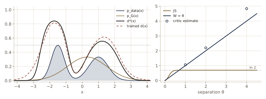
The training error settles near the population minimum (it fluctuates because each batch is a new sample), and the learned discriminator follows \(d^\star\) to within a few hundredths on average. The largest gap, about 0.08, is on the right flank of the second data bump, where \(d^\star\) falls steeply and samples are already thinning out.
Conditional GANs
The GAN so far samples from \(p(\mathbf{x})\). Often we want to choose what is generated: an image of a particular digit, or of a dog of a given breed. A conditional GAN samples from \(p(\mathbf{x} \mid \mathbf{c})\) for a conditioning vector \(\mathbf{c}\), such as a one-hot class label. Both networks receive \(\mathbf{c}\) as an extra input, the generator as \(\mathbf{g}(\mathbf{z}, \mathbf{c}, \mathbf{w})\) and the discriminator as \(d(\mathbf{x}, \mathbf{c}, \boldsymbol{\phi})\), and training uses labeled pairs \((\mathbf{x}_n, \mathbf{c}_n)\):
\[E_{\mathrm{cGAN}} = -\frac{1}{N_{\mathrm{real}}}\sum_{n \in \mathrm{real}} \ln d(\mathbf{x}_n, \mathbf{c}_n) - \frac{1}{N_{\mathrm{synth}}}\sum_{n \in \mathrm{synth}} \ln\bigl(1 - d(\mathbf{g}(\mathbf{z}_n, \mathbf{c}_n), \mathbf{c}_n)\bigr),\]where the synthetic examples use labels drawn from the label distribution of the data. The derivation above goes through for each value of \(\mathbf{c}\) separately: the optimal discriminator becomes \(p_{\mathrm{data}}(\mathbf{x} \mid \mathbf{c}) / (p_{\mathrm{data}}(\mathbf{x} \mid \mathbf{c}) + p_G(\mathbf{x} \mid \mathbf{c}))\), so a discriminator that sees the label punishes a generator that produces a good “7” when asked for a “3”. Compared with one GAN per class, one conditional GAN shares its internal representations across classes (strokes are strokes, whatever the digit) and so uses the data more efficiently. We train one on MNIST in the image section.
GAN training in practice
The training loop
The function below implements the alternating updates: one discriminator step on a batch of real points and a batch of freshly generated ones, then one generator step on another fresh batch. It returns nothing; instead it prints the discriminator error, the generator loss, and our two coverage scores every few hundred steps, and it can call a function at chosen steps (we use that to save snapshots of the samples). Both players use Adam (module 07) with a first-moment coefficient \(\beta_1 = 0.5\) rather than the default 0.9: momentum carried over from an old opponent is often harmful in a game, and this lower value became a common choice for GANs. The option "ls" selects the least-squares losses of a later section.
def ls_d_error(a_real, a_fake):
    """Least-squares discriminator loss: targets 1 for real, 0 for synthetic."""
    return 0.5 * ((a_real - 1) ** 2).mean() + 0.5 * (a_fake ** 2).mean()

def ls_g_error(a_fake):
    return 0.5 * ((a_fake - 1) ** 2).mean()

G_ERRORS = {"sat": g_error_saturating, "ns": g_error_nonsaturating, "ls": ls_g_error}

def train_gan(g_net, d_net, g_loss="ns", steps=2000, B=128, lr=1e-3, seed=0,
              log_every=250, callback=None, callback_steps=()):
    gen = torch.Generator().manual_seed(seed)
    opt_g = torch.optim.Adam(g_net.parameters(), lr=lr, betas=(0.5, 0.999))
    opt_d = torch.optim.Adam(d_net.parameters(), lr=lr, betas=(0.5, 0.999))
    z_eval = torch.randn(2000, M, generator=torch.Generator().manual_seed(1234))
    d_err = ls_d_error if g_loss == "ls" else d_error
    for step in range(steps + 1):
        if step in callback_steps:
            callback(step, g_net, d_net)
        # discriminator: one descent step on real and freshly generated points
        x_real = sample_data(B, gen)
        with torch.no_grad():
            x_fake = g_net(torch.randn(B, M, generator=gen))
        E_d = d_err(d_net(x_real), d_net(x_fake))
        opt_d.zero_grad()
        E_d.backward()
        opt_d.step()
        # generator: one step on a new batch; the gradient flows back through d_net
        # (it also fills d_net's .grad, which the next opt_d.zero_grad() clears)
        E_g = G_ERRORS[g_loss](d_net(g_net(torch.randn(B, M, generator=gen))))
        opt_g.zero_grad()
        E_g.backward()
        opt_g.step()
        if log_every and step % log_every == 0:
            with torch.no_grad():
                modes, quality = coverage(g_net(z_eval))
            print(f"step {step:5d}   E_d {E_d.item():.3f}   E_g {E_g.item():.3f}   "
                  f"modes {modes}   good {quality:.3f}")
Now train a freshly initialized pair of networks with the non-saturating generator loss (the next section explains the choice) and keep snapshots of 300 samples for the figure.
snapshots = {}
def keep_samples(step, g_net, d_net):
    z_snap = torch.randn(300, M, generator=torch.Generator().manual_seed(5))
    with torch.no_grad():
        snapshots[step] = g_net(z_snap)

torch.manual_seed(0)
g_net, d_net = mlp(M, 2), mlp(2, 1)
t0 = time.time()
train_gan(g_net, d_net, g_loss="ns", steps=2000, callback=keep_samples,
          callback_steps=(0, 250, 500, 1000, 2000))
print(f"training time {time.time() - t0:.1f} s  (your times will differ)")
step     0   E_d 1.386   E_g 0.579   modes 0   good 0.000
step   250   E_d 1.122   E_g 0.954   modes 0   good 0.055
step   500   E_d 0.946   E_g 1.164   modes 5   good 0.248
step   750   E_d 1.137   E_g 1.122   modes 6   good 0.544
step  1000   E_d 1.213   E_g 1.210   modes 6   good 0.700
step  1250   E_d 1.196   E_g 1.028   modes 6   good 0.761
step  1500   E_d 1.331   E_g 0.910   modes 6   good 0.811
step  1750   E_d 1.354   E_g 0.888   modes 6   good 0.830
step  2000   E_d 1.332   E_g 0.933   modes 6   good 0.860
training time 8.1 s  (your times will differ)
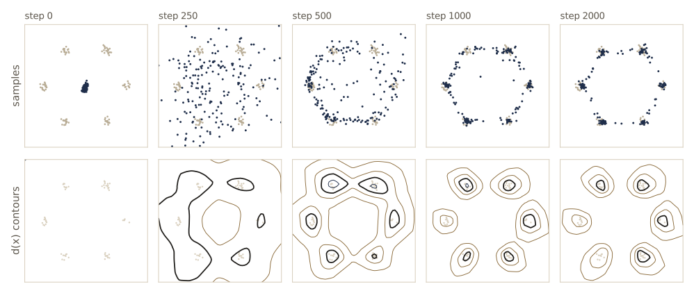
A few things to notice.
- The losses do not measure progress. The discriminator error starts near \(\ln 4 \approx 1.39\) (an untrained classifier that outputs about \(\tfrac{1}{2}\)), drops while the discriminator gets ahead, and then climbs back toward \(\ln 4\) as the generator catches up. The generator loss moves in the opposite direction. Neither decreases steadily, and a low discriminator error can mean either a bad generator or a discriminator that is too strong. With a likelihood-based model we would watch the validation log likelihood; a GAN has no such number, which is why we wrote
coverage. - Coverage and quality arrive at different times. After 250 steps the samples are scattered everywhere and no mode is covered; by step 500 the samples form a ring through five of the six modes, but only a quarter of them are good; from step 750 all six modes are covered, and the good fraction keeps rising (to 0.86 at step 2000) as the samples tighten around the centers.
- Some samples fall between modes. The generator is a continuous function of a connected latent space, so it cannot map the Gaussian \(p(\mathbf{z})\) onto six separate islands without sending a little mass across the gaps between them. More capacity makes the bridges thinner but never removes them.
Watch out. Numbers like these vary with the seed, the learning rates, and the network sizes much more than for a supervised model of the same size. A GAN result from one run is an anecdote; before you trust a comparison between two training methods, repeat it over several seeds (exercise 5 asks you to).
Saturation and the non-saturating loss
The generator’s term in \(E_{\mathrm{GAN}}\) has a flaw that shows up exactly when the generator most needs help. Write the discriminator’s output on a synthetic point as \(d = \sigma(a)\), with \(a\) the logit, and differentiate the generator’s per-sample objective with respect to \(a\) (every gradient the generator receives passes through this factor). For the original form, whose negative the generator minimizes,
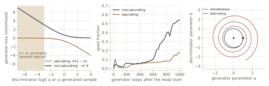
\[\frac{\partial}{\partial a}\ln\bigl(1 - \sigma(a)\bigr) = -\sigma(a) = -d,\]using \(\sigma'(a) = \sigma(a)(1 - \sigma(a))\). Early in training the generator is poor, the discriminator rejects its samples confidently, \(d \approx 0\), and so the gradient is nearly zero. The generator’s loss is flat, or saturated, precisely where it is worst.
The fix, already proposed in the original GAN paper, is to change the generator’s objective from “make the discriminator’s probability of fake small” to “make its probability of real large”: minimize
\[-\frac{1}{N_{\mathrm{synth}}}\sum_{n \in \mathrm{synth}} \ln d(\mathbf{g}(\mathbf{z}_n, \mathbf{w}), \boldsymbol{\phi})\]instead. This is the non-saturating generator loss. Its derivative with respect to the logit is
\[\frac{\partial}{\partial a}\bigl(-\ln\sigma(a)\bigr) = -(1 - \sigma(a)) = -(1 - d),\]which is close to \(-1\) when \(d \approx 0\) and vanishes only when the discriminator is fooled. Both objectives push \(d\) up and have the same fixed point, but they weight samples very differently: the original one listens to the samples that already fool the discriminator, the non-saturating one to the samples that do not. The discriminator’s loss is unchanged, so the game is no longer exactly zero-sum, and the Jensen–Shannon analysis above no longer describes the generator’s objective exactly (Arjovsky and Bottou showed that against the optimal discriminator the non-saturating loss corresponds to a combination of a reverse KL divergence and the JS divergence).
To see the effect, give the discriminator a head start: train it alone for 300 steps against an untrained generator, so it rejects the generator’s samples confidently, then compare the gradient that each loss sends to the generator’s parameters from exactly the same state.
import copy

torch.manual_seed(0)
g_start, d_start = mlp(M, 2), mlp(2, 1)
gen = torch.Generator().manual_seed(7)
opt = torch.optim.Adam(d_start.parameters(), lr=1e-3, betas=(0.5, 0.999))
for step in range(300):                                  # the discriminator gets a head start
    with torch.no_grad():
        x_fake = g_start(torch.randn(128, M, generator=gen))
    E = d_error(d_start(sample_data(128, gen)), d_start(x_fake))
    opt.zero_grad()
    E.backward()
    opt.step()
z = torch.randn(512, M, generator=gen)
with torch.no_grad():
    d_fake = torch.sigmoid(d_start(g_start(z)))
print(f"discriminator error {E.item():.4f}   "
      f"median d on generated points {d_fake.median().item():.4f}")
for name in ["sat", "ns"]:
    g_start.zero_grad()
    G_ERRORS[name](d_start(g_start(z))).backward()
    grad_norm = torch.sqrt(sum((p.grad ** 2).sum() for p in g_start.parameters()))
    print(f"{name:>3}: norm of the gradient with respect to w = {grad_norm.item():.5f}")
discriminator error 0.0031   median d on generated points 0.0020
sat: norm of the gradient with respect to w = 0.00259
 ns: norm of the gradient with respect to w = 1.09108
With the discriminator this confident, the saturating loss delivers a gradient hundreds of times smaller than the non-saturating one, from the same networks and the same latent samples. Now continue the game from this state with each loss, for 1000 steps, with identical data and latent samples.
def continue_game(g_loss, steps=1000, seed=11):
    g, d = copy.deepcopy(g_start), copy.deepcopy(d_start)
    train_gan(g, d, g_loss=g_loss, steps=steps, seed=seed, log_every=250)

t0 = time.time()
print("saturating generator loss")
continue_game("sat")
print("non-saturating generator loss")
continue_game("ns")
print(f"time {time.time() - t0:.1f} s  (your times will differ)")
saturating generator loss
step     0   E_d 0.003   E_g -0.002   modes 0   good 0.000
step   250   E_d 1.047   E_g -0.597   modes 0   good 0.036
step   500   E_d 1.007   E_g -0.447   modes 0   good 0.063
step   750   E_d 0.716   E_g -0.393   modes 1   good 0.079
step  1000   E_d 0.753   E_g -0.407   modes 3   good 0.178
non-saturating generator loss
step     0   E_d 0.003   E_g 6.290   modes 0   good 0.000
step   250   E_d 1.156   E_g 0.906   modes 0   good 0.058
step   500   E_d 0.909   E_g 1.466   modes 0   good 0.076
step   750   E_d 0.839   E_g 1.654   modes 3   good 0.294
step  1000   E_d 0.950   E_g 1.400   modes 5   good 0.544
time 7.6 s  (your times will differ)
After 1000 steps the non-saturating generator covers five modes with more than half of its samples good; the saturating one covers three, with fewer than a fifth of its samples good, and for its first 750 steps it covered at most one mode. That the saturating version moves at all is thanks to Adam, which divides each update by a running estimate of the gradient’s size and so partly undoes the shrinking; plain gradient descent at the same learning rate would move the parameters by only about \(10^{-3} \times 0.003 \approx 3 \times 10^{-6}\) per step. Even so, a tiny gradient is mostly noise, and the direction it points in is unreliable. For this reason essentially every GAN implementation uses the non-saturating loss (or one of the alternatives below) for the generator.
Mode collapse
The most characteristic failure of GANs is mode collapse: the generator maps most or all latent vectors to a small part of the data distribution, for instance to only a few of our six clusters, or, for digits, to only one digit class, drawn well. The discriminator cannot see diversity in a single sample; it judges samples one at a time, so a generator that produces a perfect “3” every time gives it nothing to reject on any single example. The discriminator then learns to reject that mode, the generator hops to another one, and the pair can chase each other around the modes without ever covering all of them. Partial collapse, where some modes are dropped for good, is common and harder to notice.
Two views explain why it happens. In the game view, the generator’s update assumes the current discriminator is fixed, and against a fixed discriminator the best response is to put all samples at the single point the discriminator likes most; only the discriminator’s later reaction makes diversity pay. In the divergence view, the non-saturating loss behaves like a reverse KL divergence \(\mathrm{KL}(p_G \Vert p_{\mathrm{data}})\), which punishes samples where the data have no mass heavily and missing modes lightly (the mode-seeking behavior of the reverse KL that module 02 demonstrates on a two-mode density). Remedies include giving the discriminator information about whole batches (for example the spread of features across the batch), the Wasserstein objective below, and architectural choices in image GANs; none is a complete cure. In our CycleGAN experiment near the end of the module we will see a clean case of mode collapse in a translation network.
Why games are hard to optimize
Even without collapse, simultaneous gradient steps on a game need not converge. The smallest example has one parameter per player: the generator’s parameter \(a\) ascends and the discriminator’s parameter \(b\) descends the error \(E(a, b) = ab\). The only equilibrium is \((0, 0)\). The gradient field \((\partial E/\partial a, -\partial E/\partial b) = (b, -a)\) is a pure rotation around it, so the players circle the equilibrium instead of approaching it. With simultaneous discrete steps,
\[\begin{pmatrix} a_{k+1} \\ b_{k+1} \end{pmatrix} = \begin{pmatrix} 1 & \eta \\ -\eta & 1 \end{pmatrix}\begin{pmatrix} a_k \\ b_k \end{pmatrix}, \qquad a_{k+1}^2 + b_{k+1}^2 = (1 + \eta^2)(a_k^2 + b_k^2),\]so the distance from the equilibrium grows by a factor \(\sqrt{1 + \eta^2}\) every step: the iterates spiral outward. If the players alternate, and the discriminator reacts to the generator’s new value, the update matrix becomes \(\begin{pmatrix} 1 & \eta \\ -\eta & 1 - \eta^2 \end{pmatrix}\), with determinant 1: it preserves area and, for \(\eta < 2\), keeps the iterates on a fixed ellipse around the equilibrium, neither approaching it nor escaping. Bishop & Bishop exercise 17.2 shows the continuous-time version of this circling.
eta, n = 0.1, 200
for scheme in ["simultaneous", "alternating"]:
    a, b = 1.0, 0.0
    radii = [1.0]
    for k in range(n):
        if scheme == "simultaneous":
            a, b = a + eta * b, b - eta * a
        else:
            a = a + eta * b
            b = b - eta * a
        radii.append(math.hypot(a, b))
    print(f"{scheme:>12}: distance from equilibrium after 0/50/100/150/200 steps "
          + " ".join(f"{radii[k]:.3f}" for k in range(0, n + 1, 50)))
print(f"predicted for simultaneous steps: (1 + eta^2)^(n/2) = {(1 + eta ** 2) ** (n / 2):.3f}")
simultaneous: distance from equilibrium after 0/50/100/150/200 steps 1.000 1.282 1.645 2.109 2.705
 alternating: distance from equilibrium after 0/50/100/150/200 steps 1.000 0.989 1.023 0.976 1.020
predicted for simultaneous steps: (1 + eta^2)^(n/2) = 2.705
Neither scheme reaches the equilibrium. The training loop above alternates, which is better than simultaneous steps, but a real GAN has millions of such coupled directions, and a loss that oscillates without settling is a common sight. Many practical ingredients (small learning rates, low momentum, penalties on the discriminator’s gradients, averaging the generator’s weights over time) can be read as ways of damping this rotation.
Smoother discriminators: least squares and instance noise
Saturation has a counterpart on the discriminator’s side. When \(p_{\mathrm{data}}\) and \(p_G\) barely overlap, as early in training or in high dimensions, the optimal discriminator jumps from 0 to 1 in the narrow space between them and is flat everywhere else. A flat discriminator gives the generator no direction to move, whatever loss the generator uses. Two simple ways to make the discriminator smoother:
- Least-squares GAN. Treat the discriminator output as a real number rather than a probability and replace the cross-entropy by squared errors toward targets: the discriminator minimizes \(\tfrac{1}{2}\mathbb{E}[(d(\mathbf{x}) - 1)^2] + \tfrac{1}{2}\mathbb{E}[d(\mathbf{g}(\mathbf{z}))^2]\) and the generator minimizes \(\tfrac{1}{2}\mathbb{E}[(d(\mathbf{g}(\mathbf{z})) - 1)^2]\) (the functions
ls_d_errorandls_g_errorabove). A squared error keeps growing with the distance from the target, so samples far on the wrong side still receive a gradient proportional to how wrong they are. - Instance noise. Add Gaussian noise to both the real and the synthetic samples before the discriminator sees them. Blurring both distributions makes their supports overlap, which smooths the optimal discriminator; the noise level is usually decreased during training.
Wasserstein GANs and gradient penalties
A deeper look at the same problem: the Jensen–Shannon divergence is a poor guide when the two distributions do not overlap. The next cell takes two narrow Gaussians (standard deviation 0.1) a distance \(\theta\) apart and computes JS on a grid, in log space so that the tails do not underflow.
for theta in [0.5, 1.0, 2.0, 4.0]:
    log_p = -0.5 * (xs / 0.1) ** 2 - math.log(0.1 * math.sqrt(2 * math.pi))
    log_q = -0.5 * ((xs - theta) / 0.1) ** 2 - math.log(0.1 * math.sqrt(2 * math.pi))
    log_m = torch.logaddexp(log_p, log_q) - math.log(2)
    js = (0.5 * integrate(log_p.exp() * (log_p - log_m))
          + 0.5 * integrate(log_q.exp() * (log_q - log_m)))
    print(f"theta = {theta:3.1f}   JS = {js:.4f}   (ln 2 = {math.log(2):.4f})")
theta = 0.5   JS = 0.6759   (ln 2 = 0.6931)
theta = 1.0   JS = 0.6931   (ln 2 = 0.6931)
theta = 2.0   JS = 0.6931   (ln 2 = 0.6931)
theta = 4.0   JS = 0.6931   (ln 2 = 0.6931)
Once the two bumps stop overlapping, JS is stuck at \(\ln 2\): moving the generator’s bump from 4 units away to 1 unit away does not change the objective at all, so its gradient with respect to \(\theta\) is zero. For images, which lie near thin surfaces in a space of very high dimension, non-overlapping supports are the normal situation early in training.
A distance that keeps growing with \(\theta\) is the Wasserstein distance, also called the earth mover’s distance. Picture \(p_G\) as a pile of earth and \(p_{\mathrm{data}}\) as a hole of the same volume. A transport plan says how much earth goes from each point \(\mathbf{x}\) to each point \(\mathbf{y}\); its cost is the amount moved times the distance moved, summed over all moves. The Wasserstein-1 distance is the cost of the cheapest plan:
\[W(p_{\mathrm{data}}, p_G) = \inf_{\gamma \in \Pi(p_{\mathrm{data}}, p_G)} \mathbb{E}_{(\mathbf{x}, \mathbf{y}) \sim \gamma}\bigl[\lVert \mathbf{x} - \mathbf{y} \rVert\bigr],\]where \(\Pi\) is the set of joint distributions with the two given marginals. For our two bumps the cheapest plan shifts every point by \(\theta\), so \(W = \theta\): the distance tells the generator how far it still has to go. Computing the infimum directly is hopeless in high dimensions, but the Kantorovich–Rubinstein duality rewrites it as a maximization over functions:
\[W(p_{\mathrm{data}}, p_G) = \sup_{\lVert f \rVert_L \le 1} \; \mathbb{E}_{\mathbf{x} \sim p_{\mathrm{data}}}[f(\mathbf{x})] - \mathbb{E}_{\mathbf{x} \sim p_G}[f(\mathbf{x})],\]where the supremum is over 1-Lipschitz functions, those with \(\lvert f(\mathbf{x}) - f(\mathbf{y}) \rvert \le \lVert \mathbf{x} - \mathbf{y} \rVert\) (for differentiable \(f\), gradient norm at most 1 everywhere). The maximizing \(f\) is called the critic. It plays the discriminator’s role, but it outputs an unbounded real number (no sigmoid, no log), and the Lipschitz constraint keeps it from becoming arbitrarily steep. The Wasserstein GAN trains a network \(d(\mathbf{x}, \boldsymbol{\phi})\) as the critic, maximizing the difference of means, while the generator minimizes the same difference, that is, maximizes \(\mathbb{E}[d(\mathbf{g}(\mathbf{z}))]\).
The difficulty is enforcing the constraint. The original Wasserstein GAN clipped every weight of the critic to a small interval, which bounds the gradient crudely and tends to make the critic too simple. The gradient penalty version (WGAN-GP) replaces the hard constraint by a soft one: the optimal critic has gradient norm 1 almost everywhere along the lines between matched points, so it penalizes deviations of \(\lVert\nabla_{\mathbf{x}} d\rVert\) from 1 at random points \(\hat{\mathbf{x}} = \epsilon\mathbf{x} + (1 - \epsilon)\mathbf{g}(\mathbf{z})\), \(\epsilon \sim \mathcal{U}(0, 1)\), between real and synthetic samples. The critic minimizes
\[\begin{aligned} E_{\mathrm{WGAN\text{-}GP}}(\boldsymbol{\phi}) = {} & \frac{1}{N}\sum_{n} d(\mathbf{g}(\mathbf{z}_n), \boldsymbol{\phi}) - \frac{1}{N}\sum_{n} d(\mathbf{x}_n, \boldsymbol{\phi}) \\ & + \lambda\, \frac{1}{N}\sum_{n}\bigl(\lVert \nabla_{\hat{\mathbf{x}}} d(\hat{\mathbf{x}}_n, \boldsymbol{\phi}) \rVert - 1\bigr)^2, \end{aligned}\]with \(\lambda\) (Bishop & Bishop call it \(\eta\)) controlling the penalty; \(\lambda = 10\) is the usual choice. Evaluating the penalty needs the gradient of the critic with respect to its input inside the loss, and then the gradient of that with respect to \(\boldsymbol{\phi}\): a second-order derivative, which torch.autograd.grad(..., create_graph=True) provides. Bishop & Bishop’s equation (17.11) writes a variant with the penalty evaluated at the data points; penalizing the gradient at real data is also the idea behind the R1 regularizer of Mescheder, Geiger, and Nowozin, which is widely used with the ordinary GAN loss.
Let us check the claim that the critic estimates \(W\). Place the data at the origin and the generator’s samples at distance \(\theta\) along the first axis, both with standard deviation 0.1, in two dimensions (in one dimension the penalty creates a barrier between slopes \(+1\) and \(-1\) that the optimizer cannot cross, which is a nice exercise to think about). Train a critic with the gradient penalty for each \(\theta\) and report \(\mathbb{E}_{\mathrm{data}}[d] - \mathbb{E}_G[d]\) on fresh samples.
def critic_error(d, x_real, x_fake, gen, lam=10.0):
    """WGAN-GP critic loss: mean d(fake) - mean d(real) + lam * mean (grad norm - 1)^2."""
    eps = torch.rand(len(x_real), 1, generator=gen)
    x_hat = (eps * x_real + (1 - eps) * x_fake).requires_grad_(True)
    grad = torch.autograd.grad(d(x_hat).sum(), x_hat, create_graph=True)[0]
    penalty = ((grad.norm(dim=1) - 1) ** 2).mean()
    return d(x_fake).mean() - d(x_real).mean() + lam * penalty

def fit_critic(theta, steps=600, lam=10.0):
    torch.manual_seed(3)
    gen = torch.Generator().manual_seed(4)
    shift = torch.tensor([theta, 0.0])
    critic = mlp(2, 1)
    opt = torch.optim.Adam(critic.parameters(), lr=1e-3, betas=(0.5, 0.9))
    for step in range(steps):
        x_real = 0.1 * torch.randn(256, 2, generator=gen)
        x_fake = shift + 0.1 * torch.randn(256, 2, generator=gen)
        E = critic_error(critic, x_real, x_fake, gen, lam)
        opt.zero_grad()
        E.backward()
        opt.step()
    with torch.no_grad():
        x_real = 0.1 * torch.randn(5000, 2, generator=gen)
        x_fake = shift + 0.1 * torch.randn(5000, 2, generator=gen)
        return (critic(x_real).mean() - critic(x_fake).mean()).item()

lam = 10.0
for theta in [1.0, 2.0, 4.0]:
    print(f"theta = {theta:3.1f}   critic estimate {fit_critic(theta, lam=lam):.3f}   "
          f"W = {theta:.3f}   theta + theta^2/(2 lam) = {theta + theta ** 2 / (2 * lam):.3f}")
theta = 1.0   critic estimate 1.061   W = 1.000   theta + theta^2/(2 lam) = 1.050
theta = 2.0   critic estimate 2.199   W = 2.000   theta + theta^2/(2 lam) = 2.200
theta = 4.0   critic estimate 4.838   W = 4.000   theta + theta^2/(2 lam) = 4.800
The estimates grow in proportion to \(\theta\), as \(W\) does, while JS was flat. They also overshoot \(\theta\) slightly, and the overshoot is predictable. For a critic that is linear along the first axis with slope \(s\), the loss is \(-s\theta + \lambda(s - 1)^2\), the soft penalty lets the slope exceed 1 when that pays, and minimizing over \(s\) gives \(s = 1 + \theta/(2\lambda)\) and an estimate \(s\theta = \theta + \theta^2/(2\lambda)\), the last column. The estimates are close to that value. For training a generator what matters is that the critic’s slope is about 1 between the two distributions, so the generator always gets a gradient of useful size pointing toward the data, however far away it is. Figure 2 (right) shows these estimates next to JS.
In practice. WGAN-GP usually trains the critic for several steps (five is common) per generator step, uses Adam with low momentum, and avoids batch normalization in the critic, because the penalty is defined per sample and batch normalization couples the samples of a batch. It costs about three times as much per critic step as an ordinary discriminator step because of the second derivative. On our small mixture and CPU budget it trains more slowly than the non-saturating GAN; exercise 6 asks you to run it. Its main advantages show on harder problems: a critic value that correlates with sample quality during training, and much less sensitivity to the architecture.
Image GANs
Convolutional generators and discriminators
Images are where GANs made their name. The first GANs used fully connected networks, but for images convolutional networks (module 10) are the natural choice on both sides. The discriminator is an image classifier with one output, so a standard convolutional network with strided convolutions that halve the resolution at each stage fits. The generator has the opposite shape: it maps a short latent vector to a large image. It starts with a linear layer that produces a small stack of low-resolution feature maps and then transposed convolutions with stride 2 double the resolution stage by stage while reducing the number of channels, ending in as many channels as the image has colors. The deep convolutional GAN (DCGAN) of Radford, Metz, and Chintala set out guidelines that became standard: strided convolutions instead of pooling in the discriminator, transposed convolutions in the generator, batch normalization in both networks (but not on the generator’s output or the discriminator’s input), ReLU in the generator with a \(\tanh\) output so that pixel values lie in \((-1, 1)\), and leaky ReLU in the discriminator so that gradients flow for negative inputs too. (Our tiny discriminator below leaves out batch normalization, which small models often do without.)
A conditional GAN for digits
We build a small conditional DCGAN for MNIST. To fit a CPU budget of a few seconds per cell, we average-pool the digits to \(14 \times 14\) pixels and keep the networks narrow: the generator’s linear layer produces 64 feature maps of \(7 \times 7\), one transposed convolution doubles them to \(14 \times 14\) with 32 channels, and a \(3 \times 3\) convolution turns those into the one-channel image. The label enters the generator as a one-hot vector appended to \(\mathbf{z}\), and the discriminator as ten constant feature maps (one per class, the one for the true class set to 1) stacked onto the image, so both networks see \(\mathbf{c}\) at their first layer. On a GPU you would use full-resolution digits, wider layers, and many more steps; the code needs no other change.
train_set = datasets.MNIST(root="data", train=True, download=True)
test_set = datasets.MNIST(root="data", train=False, download=True)
X = F.avg_pool2d(train_set.data[:6000].float().div(127.5).sub(1).unsqueeze(1), 2)   # in [-1, 1]
y = train_set.targets[:6000]
X_test = F.avg_pool2d(test_set.data[:2000].float().div(127.5).sub(1).unsqueeze(1), 2)
y_test = test_set.targets[:2000]
print("training images", tuple(X.shape), "  pixel range", X.min().item(), "to", X.max().item())

Mz = 32                                                   # latent dimension for digits

class DigitGenerator(nn.Module):
    def __init__(self):
        super().__init__()
        self.fc = nn.Linear(Mz + 10, 64 * 7 * 7)
        self.bn0 = nn.BatchNorm2d(64)
        self.up = nn.ConvTranspose2d(64, 32, 4, stride=2, padding=1)     # 7x7 -> 14x14
        self.bn1 = nn.BatchNorm2d(32)
        self.out = nn.Conv2d(32, 1, 3, padding=1)                         # 32 channels -> 1

    def forward(self, z, c_onehot):
        h = self.fc(torch.cat([z, c_onehot], dim=1)).view(-1, 64, 7, 7)
        h = F.relu(self.bn0(h))
        h = F.relu(self.bn1(self.up(h)))
        return torch.tanh(self.out(h))

class DigitDiscriminator(nn.Module):
    def __init__(self):
        super().__init__()
        self.conv1 = nn.Conv2d(1 + 10, 32, 4, stride=2, padding=1)        # 14x14 -> 7x7
        self.conv2 = nn.Conv2d(32, 64, 3, stride=2, padding=1)            # 7x7 -> 4x4
        self.fc = nn.Linear(64 * 4 * 4, 1)

    def forward(self, x, c_onehot):
        c_maps = c_onehot[:, :, None, None].expand(-1, 10, 14, 14)
        h = F.leaky_relu(self.conv1(torch.cat([x, c_maps], dim=1)), 0.2)
        h = F.leaky_relu(self.conv2(h), 0.2)
        return self.fc(h.flatten(1))                                       # logit

torch.manual_seed(0)
G_img, D_img = DigitGenerator(), DigitDiscriminator()
with torch.no_grad():
    out = G_img(torch.randn(2, Mz), F.one_hot(torch.tensor([3, 7]), 10).float())
print("generated batch", tuple(out.shape), "  generator parameters", n_params(G_img),
      "  discriminator parameters", n_params(D_img))
training images (6000, 1, 14, 14)   pixel range -1.0 to 1.0
generated batch (2, 1, 14, 14)   generator parameters 168129   discriminator parameters 25185
To judge the samples without training a separate classifier, use the crudest classifier there is: the nearest class mean, which assigns an image to the class whose average training image is closest in Euclidean distance. It is a weak classifier on real digits, but if the generator ignored the label, it would agree with the requested label only about 10% of the time. We also measure diversity within each class as the average distance between pairs of images of the same class; a collapsed generator would make this much smaller than for real digits.
class_means = torch.stack([X[y == k].mean(0) for k in range(10)]).flatten(1)

def nearest_mean(imgs):
    return torch.cdist(imgs.flatten(1), class_means).argmin(dim=1)

def within_class_spread(imgs, labels):
    """Average Euclidean distance between two images of the same class."""
    per_class = []
    for k in range(10):
        f = imgs[labels == k].flatten(1)
        dist = torch.cdist(f, f)
        per_class.append(dist.sum() / (len(f) * (len(f) - 1)))
    return torch.stack(per_class).mean().item()

acc_real = (nearest_mean(X_test) == y_test).float().mean().item()
print(f"nearest class mean on real test digits: accuracy {acc_real:.3f}   "
      f"within-class spread {within_class_spread(X_test, y_test):.2f}")
nearest class mean on real test digits: accuracy 0.757 within-class spread 7.36
The training loop is the same as before, with images and labels in place of points and with the non-saturating generator loss. The synthetic half of each discriminator batch uses the labels of the real half, so both halves have the same class mix. We train for 600 steps in three cells of 200.
opt_G = torch.optim.Adam(G_img.parameters(), lr=1e-3, betas=(0.5, 0.999))
opt_D = torch.optim.Adam(D_img.parameters(), lr=1e-3, betas=(0.5, 0.999))
gen_img = torch.Generator().manual_seed(1)
z_show = torch.randn(200, Mz, generator=torch.Generator().manual_seed(2))
c_show = torch.arange(10).repeat_interleave(20)              # 20 samples of each class

def evaluate_generator():
    G_img.eval()                                              # batch norm uses running averages
    with torch.no_grad():
        samples = G_img(z_show, F.one_hot(c_show, 10).float())
    G_img.train()
    return samples

def train_digits(steps, B=64):
    for step in range(steps):
        idx = torch.randint(0, len(X), (B,), generator=gen_img)
        x_real, c = X[idx], F.one_hot(y[idx], 10).float()
        x_fake = G_img(torch.randn(B, Mz, generator=gen_img), c)
        E_d = d_error(D_img(x_real, c), D_img(x_fake.detach(), c))
        opt_D.zero_grad()
        E_d.backward()
        opt_D.step()
        E_g = g_error_nonsaturating(D_img(x_fake, c))
        opt_G.zero_grad()
        E_g.backward()
        opt_G.step()
    samples = evaluate_generator()
    acc = (nearest_mean(samples) == c_show).float().mean().item()
    print(f"E_d {E_d.item():.3f}   E_g {E_g.item():.3f}   nearest-mean agreement {acc:.3f}   "
          f"within-class spread {within_class_spread(samples, c_show):.2f}")

t0 = time.time()
train_digits(200)
print(f"time {time.time() - t0:.1f} s  (your times will differ)")
E_d 1.404   E_g 0.767   nearest-mean agreement 0.475   within-class spread 4.21
time 9.7 s  (your times will differ)
t0 = time.time()
train_digits(200)
print(f"time {time.time() - t0:.1f} s  (your times will differ)")
E_d 1.387   E_g 0.750   nearest-mean agreement 0.830   within-class spread 6.40
time 10.0 s  (your times will differ)
t0 = time.time()
train_digits(200)
print(f"time {time.time() - t0:.1f} s  (your times will differ)")
E_d 1.310   E_g 0.762   nearest-mean agreement 0.835   within-class spread 6.00
time 9.5 s  (your times will differ)
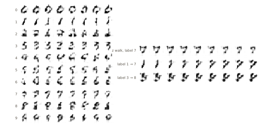
After 600 small steps most samples are recognizable digits of the requested classes, rough and blocky at \(14 \times 14\) pixels. The label is clearly used: the nearest-mean rule agrees with it on about 83% of generated digits, a little more often than on real test digits (76%). That is not a sign that the samples are better than real digits. It says that the generator favors typical shapes close to their class mean, and the within-class spread, 6.0 against 7.4 for real digits, says the same: the samples are less varied than the data, a mild form of the reduced diversity discussed under mode collapse. Watch also how the spread first collapses (4.2 after 200 steps) and then recovers as training goes on. Longer training, wider networks, and full resolution improve all of these numbers.
What the latent space learns
A GAN is trained only to produce realistic samples, yet its latent space tends to become organized. Radford and colleagues showed for DCGANs trained on photographs that walking along a straight line in latent space produces a smooth sequence of plausible images, and that some directions in latent space correspond to meaningful changes (such as the orientation of a face or whether it wears glasses); averaging the latent vectors of several images that share an attribute and doing vector arithmetic on those averages can transfer the attribute to a new image, which the same arithmetic on pixels cannot do. Representations in which separate directions control separate attributes are called disentangled. Figure 5 (right) shows the same effects in miniature: a latent walk at a fixed label, and a walk in the label input between two classes. The next cell makes the label walk and reads each image with the nearest-mean rule.
G_img.eval()
lam_grid = torch.linspace(0, 1, 9)
z_walk = torch.randn(1, Mz, generator=torch.Generator().manual_seed(3)).expand(9, -1)
with torch.no_grad():
    for a, b in [(1, 7), (3, 8)]:
        c_mix = (1 - lam_grid)[:, None] * F.one_hot(torch.tensor(a), 10) \
                + lam_grid[:, None] * F.one_hot(torch.tensor(b), 10)
        read_as = nearest_mean(G_img(z_walk, c_mix.float()))
        print(f"label blended from {a} to {b}: read as", read_as.tolist())
_ = G_img.train()
label blended from 1 to 7: read as [1, 1, 1, 1, 1, 7, 7, 7, 7]
label blended from 3 to 8: read as [5, 5, 8, 8, 8, 8, 8, 8, 8]
The generator was never shown a blended label, yet every blend produces a digit-like image, and the reading switches once along the path (from 1 to 7 at the middle of the first walk, from 5 to 8 early in the second). The first image of the second walk, generated with the pure label 3, is read as a 5: our crude classifier and our briefly trained generator both have limits, and a rough “3” at \(14 \times 14\) pixels is close to a “5”. The overall picture is still that the network has learned a continuous family of shapes rather than ten disconnected lookup tables.
Progressive growing, StyleGAN, and BigGAN
The same ingredients, scaled up and refined, produced the GANs behind the well-known photographs of people who do not exist. We describe the main ideas without numbers; the papers are listed at the end.
- Progressive growing (Karras and colleagues) starts training both networks at a very low resolution, where the global layout of an image is learned quickly and stably, and then adds layers that double the resolution, fading each new layer in gradually. The fine details are learned last, on top of a structure that is already right. This made stable training at megapixel resolution possible.
- StyleGAN (from the same group) changes the generator. A separate mapping network first transforms \(\mathbf{z}\) into an intermediate latent vector; the synthesis network starts from a learned constant rather than from \(\mathbf{z}\), and the intermediate vector sets the scale and bias of the normalized feature maps at every resolution (the “style” of that layer). Per-pixel noise inputs add stochastic detail such as the exact placement of hairs. Coarse layers then control pose and shape and fine layers control color and texture, which makes the latent space notably more disentangled and allows styles from different latent vectors to be mixed.
- BigGAN (Brock, Donahue, and Simonyan) scales class-conditional GANs to large, diverse image collections, with residual blocks, a shared class embedding that modulates batch normalization throughout the generator, a projection of the class embedding in the discriminator, very large batches, and regularization to keep training stable. Its truncation trick samples \(\mathbf{z}\) from a normal distribution with the tails cut off: this trades diversity for fidelity, with a single knob, at sampling time.
Note. How are such models compared if there is no likelihood? The standard answer is to compare statistics of generated and real images in the feature space of a pretrained classifier. The Fréchet Inception distance (FID) fits a Gaussian to the features of each set and measures the distance between the two Gaussians; lower is better. It rewards both quality and diversity, but it depends on the feature network and the sample size, so FID values are only comparable within one evaluation protocol. Our
coverageand nearest-mean scores are toy versions of the same idea.
CycleGAN
GANs can learn conditional distributions for problems that have nothing to do with classes. Image-to-image translation maps an image in one domain to a corresponding image in another: a photograph to a painting of the same scene, a summer landscape to a winter one, a horse to a zebra in the same pose. If we had many pairs of corresponding images this would be supervised learning. Usually we have only two unpaired collections, photographs in one folder and paintings in another. CycleGAN (Zhu and colleagues) learns translation from such unpaired data.
It uses two generators and two discriminators. For domains \(\mathcal{X}\) and \(\mathcal{Y}\), the generator \(\mathbf{g}_{Y}(\mathbf{x}, \mathbf{w}_Y)\) maps a point of \(\mathcal{X}\) into \(\mathcal{Y}\), and \(\mathbf{g}_{X}(\mathbf{y}, \mathbf{w}_X)\) maps back. (The subscript names the domain a generator produces.) The discriminator \(d_Y\) tells real members of \(\mathcal{Y}\) from outputs of \(\mathbf{g}_Y\), and \(d_X\) does the same in \(\mathcal{X}\). Here the generators take a data point, not random noise, as input; the randomness of the ordinary GAN is replaced by the variety of the input domain.
The two GAN losses alone make the outputs look like members of the target domain, but they say nothing about which output belongs to which input: any map that turns the distribution of \(\mathcal{X}\) into the distribution of \(\mathcal{Y}\) is a perfect solution, however it pairs individual inputs with outputs, and in practice training may not even reach such a map but collapse several parts of \(\mathcal{X}\) onto one part of \(\mathcal{Y}\). CycleGAN adds the requirement that translating there and back returns the original. The cycle-consistency error is
\[E_{\mathrm{cyc}}(\mathbf{w}_X, \mathbf{w}_Y) = \frac{1}{N_X}\sum_{n \in \mathcal{X}} \lVert \mathbf{g}_X(\mathbf{g}_Y(\mathbf{x}_n)) - \mathbf{x}_n \rVert_1 + \frac{1}{N_Y}\sum_{n \in \mathcal{Y}} \lVert \mathbf{g}_Y(\mathbf{g}_X(\mathbf{y}_n)) - \mathbf{y}_n \rVert_1,\]with the \(L_1\) norm \(\lVert \mathbf{v} \rVert_1 = \sum_i \lvert v_i \rvert\), and the generators are trained on the total
\[E_{\mathrm{GAN}}(\mathbf{w}_X, \boldsymbol{\phi}_X) + E_{\mathrm{GAN}}(\mathbf{w}_Y, \boldsymbol{\phi}_Y) + \lambda\, E_{\mathrm{cyc}}(\mathbf{w}_X, \mathbf{w}_Y),\]where \(\lambda\) (again \(\eta\) in Bishop & Bishop) weighs the two goals. Each training example contributes four terms: for a point \(\mathbf{x}_n\), the adversarial term of \(\mathbf{g}_Y(\mathbf{x}_n)\) judged by \(d_Y\) and the cycle term of \(\mathbf{g}_X(\mathbf{g}_Y(\mathbf{x}_n))\); for a point \(\mathbf{y}_n\), the mirror image. A map that can be undone must keep enough information about its input to reconstruct it, so cycle consistency pushes \(\mathbf{g}_Y\) and \(\mathbf{g}_X\) toward a pair of mutually inverse, one-to-one maps between the domains. The original CycleGAN uses the least-squares adversarial loss, convolutional generators with residual blocks, and discriminators that classify overlapping image patches rather than whole images.
A CycleGAN on two toy domains
We define two domains in the plane, each a mixture of four tight clusters. Domain \(\mathcal{X}\) has its clusters at the corners of a square, \((\pm 1, \pm 1)\); domain \(\mathcal{Y}\) has them at \((\pm 2, 0)\) and \((0, \pm 2)\), a larger square turned by 45 degrees. Nothing says which cluster of \(\mathcal{X}\) should correspond to which cluster of \(\mathcal{Y}\); each corner of \(\mathcal{X}\) is equally close to two clusters of \(\mathcal{Y}\). A good translation should at least be a one-to-one matching of clusters that the reverse map undoes. We train all four networks with the least-squares losses from before, once without the cycle term (\(\lambda = 0\)) and once with it (\(\lambda = 5\)), from the same initialization.
CX = torch.tensor([[1.0, 1.0], [-1.0, 1.0], [-1.0, -1.0], [1.0, -1.0]])    # clusters of X
CY = torch.tensor([[2.0, 0.0], [0.0, 2.0], [-2.0, 0.0], [0.0, -2.0]])      # clusters of Y

def sample_domain(centers, n, gen):
    k = torch.randint(0, len(centers), (n,), generator=gen)
    return centers[k] + 0.15 * torch.randn(n, 2, generator=gen), k

x_eval, k_eval = sample_domain(CX, 1000, torch.Generator().manual_seed(99))

def train_cyclegan(lam, steps=800, B=128, seed=0):
    torch.manual_seed(seed)
    gen = torch.Generator().manual_seed(seed + 5)
    g_X, g_Y, d_X, d_Y = mlp(2, 2), mlp(2, 2), mlp(2, 1), mlp(2, 1)   # g_Y: X -> Y, g_X: Y -> X
    opt_g = torch.optim.Adam([*g_X.parameters(), *g_Y.parameters()], lr=1e-3, betas=(0.5, 0.999))
    opt_d = torch.optim.Adam([*d_X.parameters(), *d_Y.parameters()], lr=1e-3, betas=(0.5, 0.999))
    for step in range(steps + 1):
        x, _ = sample_domain(CX, B, gen)
        y, _ = sample_domain(CY, B, gen)
        with torch.no_grad():
            y_fake, x_fake = g_Y(x), g_X(y)
        E_d = ls_d_error(d_Y(y), d_Y(y_fake)) + ls_d_error(d_X(x), d_X(x_fake))
        opt_d.zero_grad()
        E_d.backward()
        opt_d.step()
        y_fake, x_fake = g_Y(x), g_X(y)
        E_adv = ls_g_error(d_Y(y_fake)) + ls_g_error(d_X(x_fake))
        E_cyc = ((g_X(y_fake) - x).abs().sum(1).mean()          # x -> y -> x
                 + (g_Y(x_fake) - y).abs().sum(1).mean())       # y -> x -> y
        E_g = E_adv + lam * E_cyc
        opt_g.zero_grad()
        E_g.backward()
        opt_g.step()
    return g_X, g_Y

def report(g_X, g_Y):
    with torch.no_grad():
        y_out = g_Y(x_eval)
        x_back = g_X(y_out)
    k_out = torch.cdist(y_out, CY).argmin(1)                    # which Y cluster each x lands in
    k_back = torch.cdist(x_back, CX).argmin(1)                  # which X cluster it returns to
    table = torch.zeros(4, 4, dtype=torch.long)
    table.index_put_((k_eval, k_out), torch.ones_like(k_eval), accumulate=True)
    print("rows: cluster of x;  columns: cluster of g_Y(x) in Y")
    print(table.numpy())
    print(f"mean L1 round-trip error {(x_back - x_eval).abs().sum(1).mean().item():.3f}   "
          f"fraction returned to their own cluster {(k_back == k_eval).float().mean().item():.3f}")
t0 = time.time()
g_X0, g_Y0 = train_cyclegan(lam=0.0)
print("without the cycle term (lambda = 0)")
report(g_X0, g_Y0)
print(f"time {time.time() - t0:.1f} s  (your times will differ)")
without the cycle term (lambda = 0)
rows: cluster of x;  columns: cluster of g_Y(x) in Y
[[  0   0 242   0]
 [  0   0   0 252]
 [  0   0   0 234]
 [  0   0 272   0]]
mean L1 round-trip error 3.234   fraction returned to their own cluster 0.000
time 6.5 s  (your times will differ)
t0 = time.time()
g_X5, g_Y5 = train_cyclegan(lam=5.0)
print("with the cycle term (lambda = 5)")
report(g_X5, g_Y5)
print(f"time {time.time() - t0:.1f} s  (your times will differ)")
with the cycle term (lambda = 5)
rows: cluster of x;  columns: cluster of g_Y(x) in Y
[[  0   0 242   0]
 [  0 252   0   0]
 [234   0   0   0]
 [  0   0   0 272]]
mean L1 round-trip error 0.033   fraction returned to their own cluster 1.000
time 7.3 s  (your times will differ)
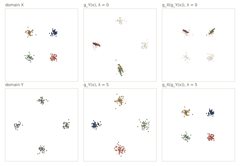
The results are exactly the failure and the fix described above. Without the cycle term, the adversarial losses are satisfied only partially: \(\mathbf{g}_Y\) has collapsed, sending pairs of \(\mathcal{X}\) clusters onto the same \(\mathcal{Y}\) cluster and leaving others empty, a clean small example of mode collapse, and since \(\mathbf{g}_X\) was trained independently, the round trip returns no point at all to its own cluster. With the cycle term the translation is a one-to-one matching of clusters, and the round trip reproduces the input with a small error. Which matching it found is arbitrary: the domains are symmetric, and a different seed can give a different, equally valid matching.
Watch out. Cycle consistency makes the two maps invertible, not correct. When the domains have symmetries, several invertible matchings fit equally well, and nothing in the loss prefers the one a human would call right (here, any rotation or reflection of the matching). In real applications the network’s inductive bias (convolutions that keep things in place, residual generators that start near the identity) does much of the work of choosing a sensible translation. Cycle-consistent networks have also been observed to hide the information needed for reconstruction in small, nearly invisible perturbations of their outputs, which satisfies the loss without a meaningful correspondence.
Summary
| Method or idea | What it does | Key equation or property |
|---|---|---|
| GAN | trains an implicit generator against a classifier | \(\min_{\boldsymbol{\phi}}\max_{\mathbf{w}} E_{\mathrm{GAN}}\); discriminator descends, generator ascends |
| Optimal discriminator | best classifier for a fixed generator | \(d^\star = p_{\mathrm{data}}/(p_{\mathrm{data}} + p_G)\) |
| Generator’s objective against \(d^\star\) | distance between model and data | \(C(p_G) = \ln 4 - 2\,\mathrm{JS}(p_{\mathrm{data}} \Vert p_G)\), best at \(p_G = p_{\mathrm{data}}\) |
| Non-saturating loss | strong gradient when the generator is poor | minimize \(-\ln d(\mathbf{g}(\mathbf{z}))\); \(\partial/\partial a = -(1 - d)\) instead of \(-d\) |
| Conditional GAN | samples from \(p(\mathbf{x} \mid \mathbf{c})\) | \(\mathbf{c}\) is an input to both networks |
| Least-squares GAN, instance noise | smoother discriminator | squared error toward targets; noise on both inputs |
| WGAN-GP | Wasserstein distance with a critic | critic maximizes \(\mathbb{E}_{\mathrm{data}}[d] - \mathbb{E}_G[d]\) with penalty \(\lambda(\lVert\nabla d\rVert - 1)^2\) |
| DCGAN | convolutional image GAN | strided convolutions in \(d\), transposed convolutions in \(\mathbf{g}\), batch norm |
| CycleGAN | unpaired translation between two domains | \(E_{\mathrm{GAN}}^{X} + E_{\mathrm{GAN}}^{Y} + \lambda E_{\mathrm{cyc}}\), \(E_{\mathrm{cyc}}\) an \(L_1\) round-trip error |
Ideas to carry forward:
- A classifier trained to separate data from model samples is a learned measure of discrepancy, and it estimates the density ratio between them. GANs use it as a loss for a model whose likelihood is unavailable.
- A game is not an optimization problem. Losses need not decrease, simultaneous gradient steps can circle or diverge, and the generator can satisfy each judgment of the discriminator while dropping modes. Most practical GAN techniques exist to tame these dynamics.
- What the generator learns depends on how the discrepancy is measured: JS saturates for non-overlapping distributions, least squares and Wasserstein distances keep a gradient that points toward the data.
- Adversarial losses make outputs look right; extra terms such as cycle consistency (or a reconstruction or conditioning input) are needed to make them correspond to something. The same idea returns whenever a GAN loss is added to another model, for example to sharpen the outputs of autoencoders (module 19).
Exercises
- Show that for fixed \(p_{\mathrm{data}}\) and \(p_G\) the population error \(E(p_G, d)\) is a convex functional of \(d\), and that \(E(p_G, d^\star) \le \ln 4\) for every \(p_G\). For what \(p_G\) can a discriminator do no better than the constant \(d = \tfrac{1}{2}\)?
- Suppose the data distribution is an equal mixture of three well-separated classes and the generator has learned to produce only the first class, perfectly, and never the other two. Using \(d^\star\), find the optimal discriminator output on a real image of the first class, and on real images of the other classes. What does the non-saturating generator loss push the generator to do from this state?
- Prove that \(0 \le \mathrm{JS}(p \Vert q) \le \ln 2\), that the upper bound is attained exactly when \(p\) and \(q\) have disjoint supports, and that JS is symmetric in its two arguments. Then compute the gradient of \(C(p_G)\) with respect to the generator’s shift \(\theta\) for the two narrow Gaussians of the Wasserstein section, and explain in one sentence why it vanishes.
- For a discriminator logit \(a\), plot (or tabulate) the per-sample generator gradients \(-d\) and \(-(1 - d)\) of the saturating and non-saturating losses against \(d\), and the least-squares generator gradient \(a - 1\) against \(a\). Which of the three gives the largest gradient to samples that the discriminator rejects most confidently?
- Repeat the mixture GAN of the notes with five different seeds for each of the losses
"sat","ns", and"ls", and report the mean and range of the number of modes covered and of the good fraction after 2000 steps. Is the difference between the losses larger or smaller than the variation across seeds? - Write a
train_wganfunction for the mixture that usescritic_errorfor the critic (five critic steps per generator step, Adam with \(\beta_1 = 0.5\), \(\beta_2 = 0.9\)) and the generator loss \(-\mathbb{E}[d(\mathbf{g}(\mathbf{z}))]\). Train it for as many generator steps as your budget allows, log the critic’s estimate \(\mathbb{E}_{\mathrm{data}}[d] - \mathbb{E}_G[d]\) alongsidecoverage, and compare how the estimate and the good fraction move together. - Repeat the one-dimensional version of
fit_critic(data at 0, generator at \(\theta\), both on a line) from several seeds. Show that for some seeds the critic ends with slope near \(-1\) and a negative estimate. Explain, using the penalty \(\lambda(\lvert f'\rvert - 1)^2\) along the path from slope \(-1\) to slope \(+1\), why gradient descent cannot fix this in one dimension but can in two. - Analyze the bilinear game \(E(a, b) = ab\) with alternating updates: find the eigenvalues of the update matrix \(\begin{pmatrix} 1 & \eta \\ -\eta & 1 - \eta^2 \end{pmatrix}\), show that they have modulus 1 for \(0 < \eta < 2\), and find a quadratic quantity that the alternating iteration conserves exactly. What happens for \(\eta > 2\)?
- Add instance noise to the mixture GAN: add Gaussian noise of standard deviation \(\sigma_{\mathrm{inst}}\) to both real and generated points before the discriminator, with \(\sigma_{\mathrm{inst}}\) decreasing linearly from 0.5 to 0 during training. Repeat the head-start experiment of the saturation section with the saturating loss and instance noise. Does the noise rescue the saturating generator? Why?
- Extend the conditional digit GAN with a third convolutional stage to generate full \(28 \times 28\) digits, and compare nearest-mean agreement and within-class spread after the same number of steps. Then remove the label from the discriminator only (it still reaches the generator) and explain what happens to the agreement.
- In the toy CycleGAN, replace domain \(\mathcal{Y}\) by eight clusters on a circle while \(\mathcal{X}\) keeps four. Can a pair of maps be both cycle consistent and a perfect GAN solution? Train with \(\lambda = 5\) and describe what the networks do instead.
- In your own words: explain to a classmate why a GAN can learn a data distribution without ever evaluating a probability density, what the discriminator is really estimating, and why training can fail even when both networks are large enough to represent the solution.
Going further
- C. M. Bishop and H. Bishop, Deep Learning: Foundations and Concepts, chapter 17 — the source for this module. Exercise 17.1 is the full optimal-discriminator and Jensen–Shannon derivation, 17.2 the continuous-time analysis of the bilinear game, and 17.3 a short calculation with \(d^\star\) in the spirit of exercise 2 above.
- Ian Goodfellow and colleagues, “Generative adversarial networks”, arXiv:1406.2661 — the original paper, with the minimax game, the optimal discriminator, and the non-saturating loss.
- Martin Arjovsky, Soumith Chintala, and Léon Bottou, “Wasserstein GAN”, arXiv:1701.07875; and Ishaan Gulrajani and colleagues, “Improved training of Wasserstein GANs”, arXiv:1704.00028 — the earth mover’s distance, the critic, and the gradient penalty.
- Alec Radford, Luke Metz, and Soumith Chintala, “Unsupervised representation learning with deep convolutional generative adversarial networks”, arXiv:1511.06434 — the DCGAN guidelines, latent walks, and latent vector arithmetic.
- Jun-Yan Zhu, Taesung Park, Phillip Isola, and Alexei Efros, “Unpaired image-to-image translation using cycle-consistent adversarial networks”, arXiv:1703.10593 — CycleGAN.
- Related modules: the nonlinear latent-variable model and the four approaches to deep generative modeling in module 16; the other three approaches in module 18 (normalizing flows), module 19 (variational autoencoders), and module 20 (diffusion models); and the zero-forcing and zero-avoiding directions of the KL divergence in Intro to ML, module 10.
These notes follow the chapters of C. M. Bishop and H. Bishop, Deep Learning: Foundations and Concepts (Springer, 2024), the course text, which the authors make free to read online. The explanations, code, figures, and exercises here are written for this course; the book remains the reference, with the full derivations and many more exercises.