CSE 676 · Module 19 · Week 13
Autoencoders
Linear, deep, sparse, denoising, and masked autoencoders; variational autoencoders with amortized inference and the reparameterization trick.
Companion reading: Bishop & Bishop, Deep Learning: Foundations and Concepts, chapter 19, “Autoencoders”
By the end of this module you can
- Derive the optimal linear autoencoder, show that it projects onto the principal subspace, and verify it with principal angles against PCA on MNIST.
- Build and train deep autoencoders in PyTorch and measure how reconstruction error depends on the size of the bottleneck, compared with PCA.
- Constrain a representation with an L1 penalty on activations and measure the resulting sparsity.
- Train denoising autoencoders and show that a trained denoiser, through Tweedie’s formula, estimates the score of the noise-smoothed data density.
- Implement a small masked autoencoder with a transformer encoder that sees only the visible patches, and evaluate its features with a linear probe.
- Derive the variational autoencoder’s ELBO, including the closed-form Gaussian KL term, and explain amortized inference and the gap it leaves.
- Derive the reparameterization and score-function gradient estimators and compare their variances numerically.
- Train a VAE on binarized MNIST, read its latent space, estimate its log likelihood by importance sampling, and recognize posterior collapse and blurry samples.
Contents
An autoencoder is a network trained to reproduce its own input. That sounds pointless, since the identity map does it perfectly, and it would be, except that we deliberately make the job hard: we squeeze the signal through a narrow layer, penalize busy hidden units, or damage the input and ask for the undamaged version. To succeed under such a handicap the network has to find structure in the data, and the internal layer where it records that structure is the representation we are after. Module 06 introduced representation learning and named autoencoders as one of its classic tools; this module builds them.
Every autoencoder has two halves. The encoder maps an input \(\mathbf{x}\) to a code (or latent representation) \(\mathbf{z}(\mathbf{x})\), and the decoder maps the code to an output \(\mathbf{y}(\mathbf{z})\) that should be close to \(\mathbf{x}\). The first half of the module covers deterministic autoencoders and the different constraints that keep them from learning the identity: a bottleneck (linear and deep autoencoders), a sparsity penalty, noise (denoising autoencoders), and missing patches (masked autoencoders). Along the way we meet two ideas that later modules depend on: a trained denoiser knows the gradient of the log density (module 20), and masking plus reconstruction is the same self-supervised recipe as masked language modelling (module 12).
The second half turns the autoencoder into a probabilistic generative model, the variational autoencoder (VAE). It is the nonlinear latent-variable model of module 16, trained by maximizing the evidence lower bound of module 15, with a second network that does approximate inference and a trick that lets gradients flow through random samples. It is the third of the four approaches to deep generative modelling, after GANs (module 17) and normalizing flows (module 18). All models are small enough to train on a CPU in seconds, on 6,000 MNIST digits.
import math
import numpy as np
import torch
import torch.nn as nn
import torch.nn.functional as F
from torchvision import datasets

np.set_printoptions(precision=4, suppress=True)
rng = np.random.default_rng(19)
torch.manual_seed(19)
We use the first 6,000 training images and the first 2,000 test images, flattened to vectors of \(D = 784\) intensities in \([0, 1]\), one row per image.
train_set = datasets.MNIST(root="data", train=True, download=True)
test_set = datasets.MNIST(root="data", train=False, download=True)
X = train_set.data[:6000].float().div(255.).flatten(1)       # (N, D) = (6000, 784)
y = train_set.targets[:6000]
X_test = test_set.data[:2000].float().div(255.).flatten(1)
y_test = test_set.targets[:2000]
N, D = X.shape
print(f"training images {tuple(X.shape)}, test images {tuple(X_test.shape)}")
print(f"average squared length of an image, ||x||^2: {X.pow(2).sum(1).mean():.2f}")
training images (6000, 784), test images (2000, 784)
average squared length of an image, ||x||^2: 88.40
The last number sets a scale for the reconstruction errors below: a decoder that output a blank image would have an average squared error of about that size.
Deterministic autoencoders
Train a network with \(D\) inputs and \(D\) outputs to map each training vector onto itself, by minimizing the sum-of-squares reconstruction error
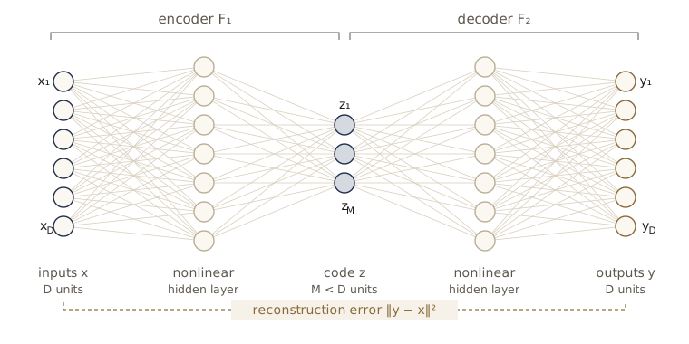
\[E(\mathbf{w}) = \frac{1}{2}\sum_{n=1}^{N} \lVert \mathbf{y}(\mathbf{x}_n, \mathbf{w}) - \mathbf{x}_n \rVert^2 .\]Such a network computes an auto-associative mapping. The targets are the inputs, so no labels are needed. If a hidden layer is at least as wide as the input and nothing else constrains the network, a perfect solution exists that has learned nothing, so we need a constraint. The simplest is a bottleneck: a hidden layer of \(M < D\) units through which all information must pass. The network then has to decide what to keep.
Linear autoencoders
Start with the smallest case: one hidden layer of \(M\) units and no nonlinearity. Write the encoder as an \(M \times D\) matrix \(\mathbf{A}\) and the decoder as a \(D \times M\) matrix \(\mathbf{B}\), so that \(\mathbf{z} = \mathbf{A}\mathbf{x}\) and \(\mathbf{y} = \mathbf{B}\mathbf{A}\mathbf{x}\). Biases only matter for the mean (the optimal output bias makes the average error zero, which is the same as centering the data), so we center the data, \(\mathbf{x}_n \leftarrow \mathbf{x}_n - \bar{\mathbf{x}}\), and drop them. With the sample covariance \(\mathbf{S} = \frac{1}{N}\sum_n \mathbf{x}_n\mathbf{x}_n^{\mathrm{T}}\), the average error per image is
\[\frac{1}{N}\sum_{n=1}^{N} \lVert \mathbf{x}_n - \mathbf{B}\mathbf{A}\mathbf{x}_n \rVert^2 = \operatorname{Tr}\left\{ (\mathbf{I} - \mathbf{B}\mathbf{A})\,\mathbf{S}\,(\mathbf{I} - \mathbf{B}\mathbf{A})^{\mathrm{T}} \right\},\]because \(\lVert \mathbf{v} \rVert^2 = \operatorname{Tr}(\mathbf{v}\mathbf{v}^{\mathrm{T}})\) and the trace is linear. Two things follow at once. The error depends on the data only through \(\mathbf{S}\), as it did for PCA. And the product \(\mathbf{B}\mathbf{A}\) has rank at most \(M\), so the network is a rank-constrained linear map. Which rank-\(M\) map is best? We find the minimum in three steps.
Step 1: the best decoder for a given encoder. For fixed \(\mathbf{A}\) the error is a least-squares problem in \(\mathbf{B}\): regress \(\mathbf{x}\) on the codes \(\mathbf{A}\mathbf{x}\). Setting the derivative with respect to \(\mathbf{B}\) to zero gives \(-2\mathbf{S}\mathbf{A}^{\mathrm{T}} + 2\mathbf{B}\mathbf{A}\mathbf{S}\mathbf{A}^{\mathrm{T}} = \mathbf{0}\), so (for \(\mathbf{A}\) of full rank \(M\) and \(\mathbf{S}\) positive definite)
\[\mathbf{B} = \mathbf{S}\mathbf{A}^{\mathrm{T}}(\mathbf{A}\mathbf{S}\mathbf{A}^{\mathrm{T}})^{-1} .\]Step 2: the error as a function of the encoder alone. Substituting, and using the fact that a least-squares residual is orthogonal to the fit, the error becomes
\[\operatorname{Tr}(\mathbf{S}) - \operatorname{Tr}\left\{ (\mathbf{A}\mathbf{S}\mathbf{A}^{\mathrm{T}})^{-1}\mathbf{A}\mathbf{S}^2\mathbf{A}^{\mathrm{T}} \right\} = \operatorname{Tr}(\mathbf{S}) - \operatorname{Tr}(\mathbf{S}\boldsymbol{\Pi}), \qquad \boldsymbol{\Pi} = \mathbf{C}^{\mathrm{T}}(\mathbf{C}\mathbf{C}^{\mathrm{T}})^{-1}\mathbf{C}, \quad \mathbf{C} = \mathbf{A}\mathbf{S}^{1/2} .\](Check it by writing \(\mathbf{A}\mathbf{S}\mathbf{A}^{\mathrm{T}} = \mathbf{C}\mathbf{C}^{\mathrm{T}}\) and \(\mathbf{A}\mathbf{S}^2\mathbf{A}^{\mathrm{T}} = \mathbf{C}\mathbf{S}\mathbf{C}^{\mathrm{T}}\) and cycling the trace.) The matrix \(\boldsymbol{\Pi}\) is the orthogonal projection onto the \(M\)-dimensional row space of \(\mathbf{C}\).
Step 3: the best projection. Minimizing the error means maximizing \(\operatorname{Tr}(\mathbf{S}\boldsymbol{\Pi})\), the variance captured by an \(M\)-dimensional subspace. That is the maximum-variance problem of PCA (module 16): the maximum is \(\lambda_1 + \dots + \lambda_M\), the sum of the \(M\) largest eigenvalues of \(\mathbf{S}\), reached when the subspace is spanned by the leading eigenvectors \(\mathbf{u}_1, \dots, \mathbf{u}_M\). Since \(\mathbf{S}^{-1/2}\) maps that span into itself, the rows of \(\mathbf{A}\) span it too, and so do the columns of \(\mathbf{B} = \mathbf{S}\mathbf{A}^{\mathrm{T}}(\cdots)^{-1}\). Then \(\mathbf{B}\mathbf{A} = \mathbf{U}_M\mathbf{U}_M^{\mathrm{T}}\).
Result. At the minimum, a linear autoencoder with \(M\) hidden units projects each input onto the principal subspace of the data, and its average error is the sum of the discarded eigenvalues, \(\sum_{i > M}\lambda_i\). The weights are not unique: for any invertible \(M \times M\) matrix \(\mathbf{G}\), the pair \((\mathbf{G}\mathbf{A}, \mathbf{B}\mathbf{G}^{-1})\) gives the same product \(\mathbf{B}\mathbf{A}\). So the columns of \(\mathbf{B}\) form a basis of the principal subspace, in general neither orthogonal nor normalized, and not the eigenvectors themselves.
Baldi and Hornik (1989) showed more: the error surface of this network has no local minima other than the global one, and every other stationary point is a saddle. We train one to see the result. Because the error depends on the data only through \(\mathbf{S}\), one full-batch gradient step costs a few small matrix products, whatever \(N\) is. First the eigen-decomposition of \(\mathbf{S}\), and a helper that measures PCA’s error at any \(M\):
x_bar = X.mean(0)
Xc = X - x_bar                                        # centered training data
S = Xc.T @ Xc / N                                     # sample covariance, (D, D)
lam, U = torch.linalg.eigh(S.double())
lam, U = lam.flip(0).float(), U.flip(1).float()       # eigenvalues in decreasing order
print("largest eigenvalues:", lam[:9].numpy().round(3))
print(f"total variance Tr(S) = {lam.sum():.2f}")

def pca_error(M, X_eval):
    """Mean over images of ||x_hat - x||^2 after projecting onto the first M principal directions."""
    U_M = U[:, :M]
    X_hat = (X_eval - x_bar) @ U_M @ U_M.T + x_bar
    return (X_hat - X_eval).pow(2).sum(1).mean().item()
largest eigenvalues: [5.305 3.876 3.286 2.912 2.486 2.353 1.755 1.545 1.455]
total variance Tr(S) = 52.84
The eigenvalues fall slowly, and several neighbors are close together. That matters for iterative training: a direction mixing \(\mathbf{u}_i\) and \(\mathbf{u}_j\) changes the error only in proportion to \(\lambda_i - \lambda_j\), so the subspace is pinned down slowly where eigenvalues nearly tie. We take \(M = 6\), where the gap to the seventh eigenvalue is comparatively wide, and minimize the error written with \(\mathbf{S}\). Expanding the trace, with \(\operatorname{Tr}(\mathbf{B}\mathbf{A}\mathbf{S}) = \sum_{ij} B_{ij}(\mathbf{A}\mathbf{S})_{ji}\) and \(\operatorname{Tr}(\mathbf{B}\mathbf{A}\mathbf{S}\mathbf{A}^{\mathrm{T}}\mathbf{B}^{\mathrm{T}}) = \operatorname{Tr}(\mathbf{B}^{\mathrm{T}}\mathbf{B}\,\mathbf{A}\mathbf{S}\mathbf{A}^{\mathrm{T}})\):
def linear_ae_error(A, B):
    """(1/N) sum_n ||x_n - B A x_n||^2 for the centered data, computed from S alone."""
    AS = A @ S                                                     # (M, D)
    return torch.trace(S) - 2 * torch.sum(B.T * AS) + torch.trace((B.T @ B) @ (AS @ A.T))

M = 6
torch.manual_seed(1)
A = (0.01 * torch.randn(M, D)).requires_grad_()                    # encoder weights
B = (0.01 * torch.randn(D, M)).requires_grad_()                    # decoder weights
A_init = A.detach().clone()                                        # kept for a check below
opt = torch.optim.Adam([A, B], lr=1e-2)
for step in range(401):
    err = linear_ae_error(A, B)
    opt.zero_grad()
    err.backward()
    opt.step()
    if step % 100 == 0:
        print(f"step {step:3d}: average error {err.item():8.4f}")
print(f"PCA, sum of the discarded eigenvalues: {lam[M:].sum():.4f}")
step   0: average error  52.8456
step 100: average error  32.6248
step 200: average error  32.6231
step 300: average error  32.6230
step 400: average error  32.6230
PCA, sum of the discarded eigenvalues: 32.6228
The trained network reaches PCA’s error. To compare subspaces rather than numbers we use principal angles: if the columns of \(\mathbf{Q}_1\) and \(\mathbf{Q}_2\) are orthonormal bases of two \(M\)-dimensional subspaces, the singular values of \(\mathbf{Q}_1^{\mathrm{T}}\mathbf{Q}_2\) are the cosines of \(M\) angles, all zero exactly when the subspaces coincide.
def principal_angles(P, Q):
    """Principal angles in degrees between the column spaces of P and Q."""
    P_orth, _ = torch.linalg.qr(P)
    Q_orth, _ = torch.linalg.qr(Q)
    cosines = torch.linalg.svdvals(P_orth.T @ Q_orth).clamp(max=1.0)
    return torch.rad2deg(torch.arccos(cosines))

with torch.no_grad():
    U_M = U[:, :M]
    print("decoder columns vs principal subspace:", principal_angles(B, U_M).numpy().round(3))
    print("encoder rows    vs principal subspace:", principal_angles(A.T, U_M).numpy().round(3))
    print(f"angle between b_1 and u_1 on their own: {principal_angles(B[:, :1], U[:, :1]).item():.1f}")
    print("B^T B, which would be the identity for an orthonormal basis:")
    print((B.T @ B).numpy())
    err_direct = (Xc - Xc @ A.T @ B.T).pow(2).sum(1).mean()
    print(f"error recomputed from the 6000 images: {err_direct:.4f}")
decoder columns vs principal subspace: [0.02  0.028 0.084 0.086 0.108 0.313]
encoder rows    vs principal subspace: [ 9.952 11.757 12.916 14.728 15.702 21.453]
angle between b_1 and u_1 on their own: 86.6
B^T B, which would be the identity for an orthonormal basis:
[[ 1.3149  0.2309 -0.0283 -0.2703 -0.1369 -0.0667]
 [ 0.2309  1.4477  0.3333  0.2482 -0.4241  0.1568]
 [-0.0283  0.3333  1.6513  0.0701  0.0241 -0.0015]
 [-0.2703  0.2482  0.0701  1.517  -0.0169  0.2573]
 [-0.1369 -0.4241  0.0241 -0.0169  2.0361 -0.4452]
 [-0.0667  0.1568 -0.0015  0.2573 -0.4452  1.6473]]
error recomputed from the 6000 images: 32.6230
The decoder behaves exactly as the result predicts: all six angles are a small fraction of a degree, while the first decoder column on its own is far from the first eigenvector and the columns are neither unit length nor orthogonal. The network has found the principal subspace and an arbitrary basis of it. Recomputing the error from the images confirms that the covariance shortcut was only a shortcut.
The encoder is another story: its rows are about 10 to 21 degrees away from the principal subspace, although the error is optimal. The derivation assumed \(\mathbf{S}\) positive definite, and for MNIST it is not. Many border pixels are zero in every image, and hundreds of other directions have almost no variance. A component of an encoder row along such a direction multiplies an input that is always (nearly) zero, so it does not change any code, it receives (nearly) zero gradient, and it keeps its random initial value. The error pins the encoder down only on the directions in which the data vary:
with torch.no_grad():
    dead = X.std(0) == 0                                  # pixels that are 0 in every training image
    print(f"pixels constant over the training set: {dead.sum().item()} of {D}")
    change = (A - A_init)[:, dead].abs().max()
    print(f"largest change of an encoder weight on those pixels: {change:.1e}")
    R = U[:, lam > 1e-2]                                  # directions with variance above 0.01
    print(f"encoder rows projected onto the {R.shape[1]} directions with variance > 0.01:")
    A_proj = R @ (R.T @ A.T)                              # rows of A projected, as columns
    print("   angles to the principal subspace:", principal_angles(A_proj, U_M).numpy().round(3))
pixels constant over the training set: 120 of 784
largest change of an encoder weight on those pixels: 0.0e+00
encoder rows projected onto the 247 directions with variance > 0.01:
   angles to the principal subspace: [0.069 0.086 0.114 0.138 0.18  0.3  ]
Once the directions the data never exercise are projected out, the encoder rows also lie in the principal subspace. The same thing happens in any network: weights attached to inputs that never vary are left where initialization put them, which is one reason weight decay (module 09) is a sensible default.
Note. Making the hidden units nonlinear does not escape PCA. Bourlard and Kamp (1988) showed that for a network with a single hidden layer and linear outputs, the minimum-error solution is still the projection onto the principal subspace, whatever the hidden activation function. There is then no reason to prefer the network: an SVD solves PCA exactly in a fixed amount of time and returns orthonormal directions ordered by variance. To get something new we need more layers.
Deep autoencoders
Now put a nonlinear hidden layer on each side of the bottleneck, as in figure 1. The encoder half, \(F_1\), is a general nonlinear map from the \(D\)-dimensional data space to the \(M\)-dimensional code; the decoder half, \(F_2\), is a general nonlinear map back. The set of all possible outputs, \(\{F_2(\mathbf{z})\}\), is an \(M\)-dimensional curved surface in data space, and the encoder assigns each input the coordinates of a nearby point on that surface. This is a nonlinear generalization of PCA, in which a flat subspace is replaced by a learned curved manifold (linear units recover PCA as a special case). The price is the usual one for deep networks: the error is no longer quadratic in the weights, training is a nonconvex optimization that can end in a poor local minimum, and \(M\) must be chosen before training.
Our deep autoencoder has layers \(784 \to 128 \to M \to 128 \to 784\), ReLU hidden units, a linear bottleneck, and sigmoid outputs, since pixel intensities lie in \([0, 1]\). We write three small helpers that the rest of the module reuses: a constructor, a mini-batch training loop that takes any loss function, and a function that measures reconstruction error.
def make_ae(M, H=128):
    """Encoder D -> H -> M and decoder M -> H -> D with ReLU hidden layers and sigmoid outputs."""
    encoder = nn.Sequential(nn.Linear(D, H), nn.ReLU(), nn.Linear(H, M))
    decoder = nn.Sequential(nn.Linear(M, H), nn.ReLU(), nn.Linear(H, D), nn.Sigmoid())
    return encoder, decoder

def params_of(*modules):
    return [p for m in modules for p in m.parameters()]

def fit(loss_fn, params, X_train, epochs, lr=1e-3, batch=100, seed=0, report=()):
    """Mini-batch Adam on loss_fn(x_batch); prints the epoch-average loss for epochs in `report`."""
    torch.manual_seed(seed)
    opt = torch.optim.Adam(params, lr=lr)
    for epoch in range(1, epochs + 1):
        perm = torch.randperm(len(X_train))
        total = 0.0
        for i in range(0, len(X_train), batch):
            xb = X_train[perm[i:i + batch]]
            loss = loss_fn(xb)
            opt.zero_grad()
            loss.backward()
            opt.step()
            total += loss.item() * len(xb)
        if epoch in report:
            print(f"  epoch {epoch:2d}: training loss {total / len(X_train):.3f}")
    return total / len(X_train)

def recon_error(encoder, decoder, X_in, X_target=None):
    """Mean over images of ||y(x_in) - x_target||^2; the target defaults to the input."""
    X_target = X_in if X_target is None else X_target
    with torch.no_grad():
        return (decoder(encoder(X_in)) - X_target).pow(2).sum(1).mean().item()

deep_ae = {}
torch.manual_seed(2)
enc, dec = make_ae(2)
print(f"parameters with M = 2: {sum(p.numel() for p in params_of(enc, dec)):,}")
fit(lambda xb: (dec(enc(xb)) - xb).pow(2).sum(1).mean(), params_of(enc, dec), X,
    epochs=8, lr=3e-3, seed=102, report=(1, 4, 8))
deep_ae[2] = (enc, dec)
print(f"M = 2: test error {recon_error(enc, dec, X_test):.2f}, "
      f"PCA with M = 2: {pca_error(2, X_test):.2f}")
parameters with M = 2: 202,258
  epoch  1: training loss 60.970
  epoch  4: training loss 40.373
  epoch  8: training loss 37.135
M = 2: test error 37.82, PCA with M = 2: 42.77
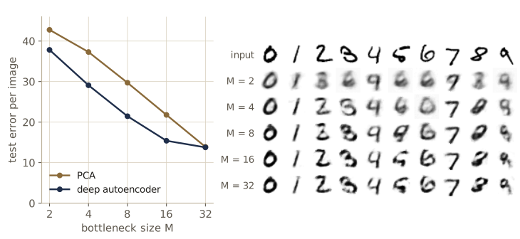
With a two-unit bottleneck the deep autoencoder already beats two principal components clearly. Now the other bottleneck sizes, each trained the same way:
for M in [4, 8, 16, 32]:
    torch.manual_seed(M)
    enc, dec = make_ae(M)
    fit(lambda xb: (dec(enc(xb)) - xb).pow(2).sum(1).mean(), params_of(enc, dec), X,
        epochs=8, lr=3e-3, seed=100 + M)
    deep_ae[M] = (enc, dec)

print(" M    deep AE (train)   deep AE (test)   PCA (test)")
for M, (enc, dec) in deep_ae.items():
    print(f"{M:2d}    {recon_error(enc, dec, X):12.2f}   {recon_error(enc, dec, X_test):14.2f}"
          f"   {pca_error(M, X_test):10.2f}")
 M    deep AE (train)   deep AE (test)   PCA (test)
 2           36.84            37.82        42.77
 4           27.80            29.09        37.30
 8           19.54            21.45        29.71
16           13.52            15.39        21.78
32           11.97            13.76        13.89
The nonlinear model wins by a wide margin when the code is tiny and the margin shrinks as \(M\) grows; by \(M = 32\) the two are about level on test data. That pattern is typical. A curved surface can follow the digits much better than a flat one of the same dimension, but with a wide bottleneck a flat subspace already captures most of the variance, and PCA’s solution is exact while our network had eight quick epochs on 6,000 images. With the full training set, a GPU, and longer training, deep autoencoders keep an edge at larger \(M\) as well (Hinton and Salakhutdinov’s 2006 paper made this case for MNIST and for documents). Figure 2 shows the reconstructions.
With \(M = 2\) we can look at the code space directly. The next cell encodes the test images and summarizes where the codes lie.
with torch.no_grad():
    z_ae = deep_ae[2][0](X_test)                        # 2-D codes of the test images
print("code range per coordinate:", z_ae.min(0).values.numpy(), "to", z_ae.max(0).values.numpy())
print("code standard deviation:  ", z_ae.std(0).numpy())
centroids = torch.stack([z_ae[y_test == k].mean(0) for k in range(10)])
print("class centroids:")
print(centroids.numpy().round(1).T)
code range per coordinate: [ -7.805  -15.7403] to [7.3764 5.7075]
code standard deviation:   [2.4321 2.8224]
class centroids:
[[-1.6 -1.8 -2.1 -2.9  1.7 -2.2 -1.   1.7 -2.7  1.6]
 [ 2.3 -3.8 -1.1 -1.1 -2.9 -1.5  0.2 -5.5 -2.1 -3.5]]
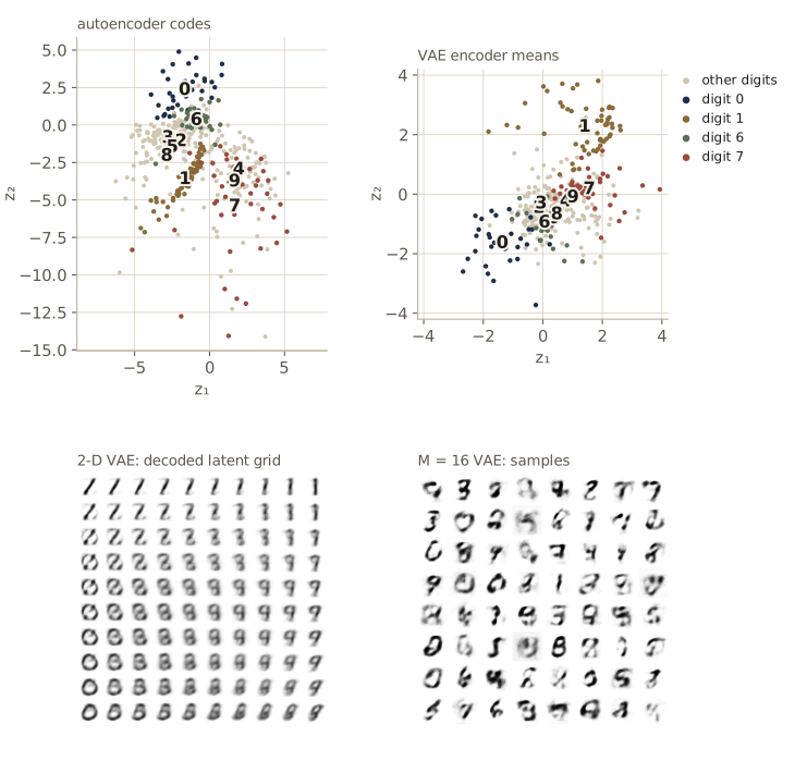
The digit classes occupy different regions (figure 6, top left, plots them), even though the network never saw a label. But the scale and placement of the code space are arbitrary: nothing in the loss prefers one layout over any stretched or bent version of it, the classes form thin rays and blobs with empty space between them, and there is no rule for which codes are “typical”. If we wanted to generate digits by choosing a code and decoding it, we would not know where to choose. For this reason plain autoencoders now play little direct role in practice; their codes are not organized in a way that later tasks or sampling can rely on. The variational autoencoder at the end of the module fixes the second problem by adding a distribution over codes.
Sparse autoencoders
A bottleneck limits the number of hidden units. An alternative is to allow many units but penalize how many are in use for each input, so that each image is described by a few active features chosen from a large dictionary. The L1 norm is the standard sparsity-inducing penalty (module 09 explains why its corners produce exact zeros). A sparse autoencoder adds it to the reconstruction error, but applied to the hidden unit activations \(z_k\) rather than to the weights:
\[\widetilde{E}(\mathbf{w}) = E(\mathbf{w}) + \lambda \sum_{k=1}^{K} \lvert z_k \rvert ,\]summed over the \(K\) units of one hidden layer (and over the data points). Automatic differentiation handles the extra term like any other. We use one hidden layer of \(K = 256\) ReLU units, so activations are nonnegative and a unit is either exactly off or on, and measure three things on the test set: how many units are on per image, how many of the largest activations are needed to account for 90% of an image’s total activation, and how many units never switch on at all.
def train_sparse_ae(lam_l1, K=256, epochs=6):
    """One hidden layer of K ReLU units, sigmoid outputs, squared error + lam_l1 * sum_k |z_k|."""
    torch.manual_seed(3)
    layer1, layer2 = nn.Linear(D, K), nn.Linear(K, D)

    def loss_fn(xb):
        z = F.relu(layer1(xb))
        return (torch.sigmoid(layer2(z)) - xb).pow(2).sum(1).mean() + lam_l1 * z.abs().sum(1).mean()

    fit(loss_fn, params_of(layer1, layer2), X, epochs, seed=4)
    with torch.no_grad():
        z = F.relu(layer1(X_test))
        err = (torch.sigmoid(layer2(z)) - X_test).pow(2).sum(1).mean().item()
        active = (z > 0).float().sum(1).mean().item()
        z_sorted = z.sort(1, descending=True).values
        share = z_sorted.cumsum(1) / z_sorted.sum(1, keepdim=True)
        k90 = ((share < 0.9).sum(1) + 1).float().mean().item()
        never = ((z > 0).sum(0) == 0).sum().item()
    return err, active, k90, never

print(" lambda   test error   units on   units for 90%   never on   (of 256)")
for lam_l1 in [0.0, 0.02, 0.05, 0.1]:
    err, active, k90, never = train_sparse_ae(lam_l1)
    print(f"  {lam_l1:4.2f}   {err:10.2f}   {active:8.1f}   {k90:13.1f}   {never:8d}")
 lambda   test error   units on   units for 90%   never on   (of 256)
  0.00        12.88      219.5           163.8         19
  0.02        13.46      150.8            89.7         24
  0.05        14.22       89.2            48.5         28
  0.10        16.07       53.2            29.6         49
Without the penalty most units respond to every digit and the activation is spread thinly over well over a hundred of them. As \(\lambda\) grows the codes become much sparser, with only a modest rise in reconstruction error, and more units are switched off for good, which lowers the effective dimension of the representation. The penalty is on activations, not parameters: it asks each input to be explained by few features, which is the idea behind sparse coding and behind the sparse dictionaries now used to interpret the internal activations of large networks.
Denoising autoencoders
A third way to rule out the identity is to change the task. A denoising autoencoder (Vincent et al., 2008) receives a corrupted copy \(\widetilde{\mathbf{x}}_n\) of each training vector and is trained to output the clean original:
\[E(\mathbf{w}) = \sum_{n=1}^{N} \lVert \mathbf{y}(\widetilde{\mathbf{x}}_n, \mathbf{w}) - \mathbf{x}_n \rVert^2 ,\]with a fresh corruption drawn every time an example is used. Common corruptions are additive Gaussian noise, \(\widetilde{\mathbf{x}} = \mathbf{x} + \sigma\boldsymbol{\epsilon}\) with \(\boldsymbol{\epsilon} \sim \mathcal{N}(\mathbf{0}, \mathbf{I})\), and masking noise, which sets a random fraction \(\nu\) of the inputs to zero. Copying the input is now useless; the network has to know what digits look like (strokes are continuous, neighboring pixels agree, a 7 has no loop) in order to undo the damage. We train one denoiser for each kind of noise, with the same architecture as the \(M = 32\) autoencoder above, and compare them with that autoencoder, which saw only clean images.
sigma, nu = 0.5, 0.5
def add_gaussian(x):
    return x + sigma * torch.randn_like(x)
def add_masking(x):
    return x * (torch.rand_like(x) > nu)                  # zero a fraction nu of the pixels

denoisers = {}
for name, corrupt, seed in [("gaussian", add_gaussian, 1), ("masking", add_masking, 3)]:
    torch.manual_seed(seed)
    enc, dec = make_ae(32)
    fit(lambda xb: (dec(enc(corrupt(xb))) - xb).pow(2).sum(1).mean(), params_of(enc, dec), X,
        epochs=8, lr=3e-3, seed=seed + 1)
    denoisers[name] = (enc, dec)

torch.manual_seed(9)
test_inputs = {"gaussian": add_gaussian(X_test), "masking": add_masking(X_test)}
print("noise      corrupted input   plain AE   Gaussian DAE   masking DAE")
for name, X_noisy in test_inputs.items():
    row = [(X_noisy - X_test).pow(2).sum(1).mean().item(), recon_error(*deep_ae[32], X_noisy, X_test),
           recon_error(*denoisers["gaussian"], X_noisy, X_test),
           recon_error(*denoisers["masking"], X_noisy, X_test)]
    print(f"{name:9s}  {row[0]:15.2f}   {row[1]:8.2f}   {row[2]:12.2f}   {row[3]:11.2f}")
print(f"clean      {0.0:15.2f}   {recon_error(*deep_ae[32], X_test):8.2f}   "
      f"{recon_error(*denoisers['gaussian'], X_test):12.2f}   "
      f"{recon_error(*denoisers['masking'], X_test):11.2f}")
with torch.no_grad():
    enc, dec = denoisers["masking"]
    print(f"total intensity per clean test image {X_test.sum(1).mean():.1f}; "
          f"masking DAE's output for it {dec(enc(X_test)).sum(1).mean():.1f}")
noise      corrupted input   plain AE   Gaussian DAE   masking DAE
gaussian            196.08      27.62          19.66         37.62
masking              40.22      31.64          25.67         19.81
clean                 0.00      13.76          15.91         29.49
total intensity per clean test image 94.8; masking DAE's output for it 137.0
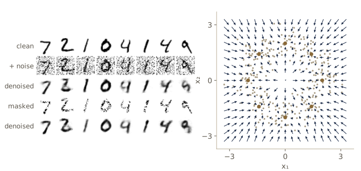
Several things to notice. The plain autoencoder is already a decent denoiser, because its bottleneck forces every output onto the learned surface of digits, and much of the noise lies off it. Each denoiser does best on the corruption it was trained for. The Gaussian denoiser generalizes reasonably: it also beats the plain autoencoder on missing pixels, and it loses little on clean inputs. The masking denoiser is a specialist. It is worse than the plain autoencoder on Gaussian noise and much worse on clean images, and the last line shows why: it was trained on inputs with half their ink removed, so it has learned to add ink, and it keeps adding it when nothing is missing. A denoiser learns the corruption as well as the data, and a mismatch between training and test corruptions costs accuracy. Figure 3 (left) shows examples.
Denoising and the score
Why does a denoiser learn structure? Bishop & Bishop §19.1.4 gives the geometric picture: data lie near a low-dimensional manifold, noise pushes a point off it, and the denoiser learns, for every point in space, a vector back toward the manifold. We can make that precise. The score of a density is the gradient of its log, \(\mathbf{s}(\mathbf{x}) = \nabla_{\mathbf{x}} \ln p(\mathbf{x})\); it points uphill toward regions of high density.
Adding Gaussian noise to data drawn from \(p(\mathbf{x})\) produces samples from the smoothed density
\[p_\sigma(\widetilde{\mathbf{x}}) = \int p(\mathbf{x})\,\mathcal{N}(\widetilde{\mathbf{x}} \mid \mathbf{x}, \sigma^2\mathbf{I})\,d\mathbf{x} .\]Differentiate under the integral. The gradient of the Gaussian with respect to its argument is \(\mathcal{N}(\widetilde{\mathbf{x}} \mid \mathbf{x}, \sigma^2\mathbf{I})\,(\mathbf{x} - \widetilde{\mathbf{x}})/\sigma^2\), so
\[\nabla p_\sigma(\widetilde{\mathbf{x}}) = \frac{1}{\sigma^2}\int (\mathbf{x} - \widetilde{\mathbf{x}})\,p(\mathbf{x})\,\mathcal{N}(\widetilde{\mathbf{x}} \mid \mathbf{x}, \sigma^2\mathbf{I})\,d\mathbf{x} = \frac{p_\sigma(\widetilde{\mathbf{x}})}{\sigma^2}\left( \mathbb{E}[\mathbf{x} \mid \widetilde{\mathbf{x}}] - \widetilde{\mathbf{x}} \right),\]where the second step recognizes \(p(\mathbf{x})\mathcal{N}(\widetilde{\mathbf{x}} \mid \mathbf{x}, \sigma^2\mathbf{I})/p_\sigma(\widetilde{\mathbf{x}})\) as the posterior \(p(\mathbf{x} \mid \widetilde{\mathbf{x}})\). Dividing by \(p_\sigma\) gives Tweedie’s formula, \(\mathbb{E}[\mathbf{x} \mid \widetilde{\mathbf{x}}] = \widetilde{\mathbf{x}} + \sigma^2\nabla \ln p_\sigma(\widetilde{\mathbf{x}})\). Finally, the function that minimizes the expected squared error \(\mathbb{E}\lVert \mathbf{r}(\widetilde{\mathbf{x}}) - \mathbf{x} \rVert^2\) is the conditional mean \(\mathbb{E}[\mathbf{x} \mid \widetilde{\mathbf{x}}]\) (the regression result of module 04). Putting the two together:
Result. If \(\mathbf{r}(\widetilde{\mathbf{x}})\) is the optimal denoiser for Gaussian noise of standard deviation \(\sigma\), then
\[\frac{\mathbf{r}(\widetilde{\mathbf{x}}) - \widetilde{\mathbf{x}}}{\sigma^2} = \nabla_{\widetilde{\mathbf{x}}} \ln p_\sigma(\widetilde{\mathbf{x}}) .\]A trained denoiser therefore estimates the score of the noise-smoothed data density, and the smaller \(\sigma\), the closer \(p_\sigma\) is to \(p\). Vincent (2011) turned this into a training principle, denoising score matching.
We check the claim where the true score is known. The data are a mixture of eight narrow Gaussians (standard deviation \(s_0 = 0.1\)) placed around a circle of radius 2, a stand-in for data near a one-dimensional manifold. Adding noise of standard deviation \(\sigma\) gives another Gaussian mixture, with variance \(\tau^2 = s_0^2 + \sigma^2\) per component, whose score is a responsibility-weighted pull toward the component means, \(\nabla \ln p_\sigma(\widetilde{\mathbf{x}}) = \sum_k \gamma_k(\widetilde{\mathbf{x}})(\boldsymbol{\mu}_k - \widetilde{\mathbf{x}})/\tau^2\). We train a small network on fresh noisy samples at every step and compare its implied score with the exact one.
K_mix, s0, sigma_toy = 8, 0.1, 0.5
angles = 2 * math.pi * torch.arange(K_mix) / K_mix
mus = 2.0 * torch.stack([angles.cos(), angles.sin()], 1)          # component means on a circle

def sample_ring(n):
    return mus[torch.randint(0, K_mix, (n,))] + s0 * torch.randn(n, 2)

def true_score(x_tilde, tau2=s0 ** 2 + sigma_toy ** 2):
    """Exact grad ln p_sigma for the noisy mixture: sum_k gamma_k (mu_k - x) / tau^2."""
    gamma = torch.softmax(-(x_tilde[:, None, :] - mus[None]).pow(2).sum(-1) / (2 * tau2), dim=1)
    return (gamma[..., None] * (mus[None] - x_tilde[:, None, :])).sum(1) / tau2

torch.manual_seed(11)
denoiser_2d = nn.Sequential(nn.Linear(2, 128), nn.SiLU(), nn.Linear(128, 128), nn.SiLU(),
                            nn.Linear(128, 2))
opt = torch.optim.Adam(denoiser_2d.parameters(), lr=2e-3)
for step in range(3001):
    x = sample_ring(512)
    x_tilde = x + sigma_toy * torch.randn_like(x)
    loss = (denoiser_2d(x_tilde) - x).pow(2).sum(1).mean()
    opt.zero_grad()
    loss.backward()
    opt.step()
    if step % 1000 == 0:
        print(f"step {step:4d}: denoising loss {loss.item():.4f}")

with torch.no_grad():
    x = sample_ring(4000)
    x_tilde = x + sigma_toy * torch.randn_like(x)
    s_learned = (denoiser_2d(x_tilde) - x_tilde) / sigma_toy ** 2
    s_true = true_score(x_tilde)
    cos = F.cosine_similarity(s_learned, s_true, dim=1)
    rel = (s_learned - s_true).norm(dim=1) / s_true.norm(dim=1)
    loss_opt = (x_tilde + sigma_toy ** 2 * s_true - x).pow(2).sum(1).mean()
    loss_net = (denoiser_2d(x_tilde) - x).pow(2).sum(1).mean()
print(f"cosine(learned score, true score): median {cos.median():.4f}, mean {cos.mean():.4f}")
print(f"relative error of the learned score: median {rel.median():.3f}")
print(f"denoising loss of the exact E[x | x~]: {loss_opt:.4f}   of the network: {loss_net:.4f}")
step    0: denoising loss 4.1214
step 1000: denoising loss 0.2506
step 2000: denoising loss 0.1979
step 3000: denoising loss 0.2415
cosine(learned score, true score): median 0.9965, mean 0.9707
relative error of the learned score: median 0.133
denoising loss of the exact E[x | x~]: 0.2215   of the network: 0.2260
The learned vectors point in almost exactly the right direction at typical noisy points, and the network’s denoising loss is within a whisker of the best achievable loss, the one obtained by Tweedie’s formula with the true score. The right panel of figure 3 draws the learned score field. This is the bridge to module 20: a diffusion model trains denoisers at many noise levels and uses the scores they imply to walk from pure noise to data.
Masked autoencoders
Masking noise with a large fraction of inputs removed is also how transformers learn language without labels: BERT-style masked language modelling hides some of the tokens of a sentence and trains the network to predict them (module 12). A masked autoencoder (MAE; He et al., 2021) carries the recipe over to images. The image is cut into patches, as in a vision transformer, a large random subset of the patches is removed, and the network is trained to reconstruct the missing ones. Three design choices distinguish it from a plain denoising autoencoder with masking noise:
- The encoder sees only the visible patches. The masked patches are dropped from the token sequence, not replaced by a placeholder. Since the cost of self-attention grows with the square of the sequence length, removing three quarters of the tokens makes the encoder much cheaper to train, which is what makes the method attractive for pre-training large vision transformers.
- Mask a lot. A missing word can change the meaning of a sentence, so language models mask a modest fraction (15% in BERT). Images are highly redundant: a missing patch can usually be filled in from its neighbors by interpolation, which teaches nothing. Masking most of the image (75% is a typical choice) forces the network to reason about the whole object.
- A light decoder that is thrown away. The decoder receives the encoded visible tokens plus one shared, learned mask token at every masked position, adds position embeddings so it knows where each token belongs, runs a smaller transformer, and maps each token to the pixel values of its patch with a linear layer. The loss is the squared error on the masked patches only. After pre-training we throw the decoder away, and the encoder, applied to complete unmasked images, becomes the starting point for downstream tasks, usually with new output layers and fine-tuning.
Our miniature MAE cuts each \(28 \times 28\) digit into a \(4 \times 4\) grid of \(7 \times 7\) patches, a sequence of 16 tokens of 49 pixels each, and keeps 4 random patches per image (75% masked). The encoder has two transformer blocks of width 64; the decoder has one block of width 32. We write the transformer block ourselves (multi-head self-attention and an MLP, each with a residual connection and a pre-layer normalization, as in module 12) so that nothing is hidden, and check our attention function once against PyTorch’s built-in.
P, G = 7, 4                           # patch side and patches per side
T = G * G                             # 16 tokens per image

def patchify(x):
    """(B, 784) images -> (B, T, P*P) patches in row-major order."""
    return x.view(-1, G, P, G, P).permute(0, 1, 3, 2, 4).reshape(-1, T, P * P)

def unpatchify(p):
    return p.view(-1, G, G, P, P).permute(0, 1, 3, 2, 4).reshape(-1, G * P * G * P)

def attention(q, k, v):
    """Scaled dot-product attention, softmax(Q K^T / sqrt(d_head)) V, for every head at once."""
    return torch.softmax(q @ k.transpose(-2, -1) / math.sqrt(q.shape[-1]), dim=-1) @ v

class Block(nn.Module):
    """Pre-norm transformer block: x + MHSA(LN(x)), then x + MLP(LN(x))."""
    def __init__(self, d, heads):
        super().__init__()
        self.ln1, self.ln2 = nn.LayerNorm(d), nn.LayerNorm(d)
        self.qkv, self.proj = nn.Linear(d, 3 * d), nn.Linear(d, d)
        self.mlp = nn.Sequential(nn.Linear(d, 2 * d), nn.GELU(), nn.Linear(2 * d, d))
        self.heads = heads

    def forward(self, x):                                            # x: (B, T, d)
        Bn, Tn, d = x.shape
        qkv = self.qkv(self.ln1(x)).view(Bn, Tn, 3, self.heads, d // self.heads)
        q, k, v = qkv.permute(2, 0, 3, 1, 4)                # each (B, heads, T, d_head)
        x = x + self.proj(attention(q, k, v).transpose(1, 2).reshape(Bn, Tn, d))
        return x + self.mlp(self.ln2(x))

class MAE(nn.Module):
    def __init__(self, d=64, d_dec=32, depth=2, heads=4):
        super().__init__()
        self.embed = nn.Linear(P * P, d)                             # patch embedding
        self.pos = nn.Parameter(0.02 * torch.randn(T, d))            # learned position embeddings
        self.blocks = nn.ModuleList([Block(d, heads) for _ in range(depth)])
        self.norm = nn.LayerNorm(d)
        self.to_dec = nn.Linear(d, d_dec)
        self.mask_token = nn.Parameter(torch.zeros(d_dec))
        self.pos_dec = nn.Parameter(0.02 * torch.randn(T, d_dec))
        self.dec_block = Block(d_dec, 2)
        self.to_pixels = nn.Linear(d_dec, P * P)

    def encode(self, patches, keep=None):
        """Encode the patches listed in keep (B, n_keep) or, if keep is None, all of them."""
        h = self.embed(patches) + self.pos
        if keep is not None:
            h = torch.gather(h, 1, keep[..., None].expand(-1, -1, h.shape[-1]))
        for blk in self.blocks:
            h = blk(h)
        return self.norm(h)

    def forward(self, patches, keep):
        h = self.to_dec(self.encode(patches, keep))                  # (B, n_keep, d_dec)
        full = self.mask_token.expand(len(patches), T, -1).clone()   # mask token everywhere ...
        full = full.scatter(1, keep[..., None].expand(-1, -1, h.shape[-1]), h)  # ... except visible
        return self.to_pixels(self.dec_block(full + self.pos_dec))   # (B, T, P*P)

def random_keep(n_images, n_keep):
    return torch.rand(n_images, T).argsort(1)[:, :n_keep]           # a random subset per image

n_keep = 4
print("patchify is invertible:", torch.equal(unpatchify(patchify(X[:10])), X[:10]))
q_, k_, v_ = torch.randn(3, 2, 4, T, 16).unbind(0)                   # (batch, heads, tokens, d_head)
print("attention matches F.scaled_dot_product_attention:",
      torch.allclose(attention(q_, k_, v_), F.scaled_dot_product_attention(q_, k_, v_), atol=1e-6))
torch.manual_seed(5)
mae = MAE()
print(f"MAE parameters: {sum(p.numel() for p in mae.parameters()):,}")
patchify is invertible: True
attention matches F.scaled_dot_product_attention: True
MAE parameters: 84,081
The loss reconstructs every patch but scores only the masked ones:
def mae_loss(xb):
    patches = patchify(xb)
    keep = random_keep(len(xb), n_keep)
    pred = mae(patches, keep)
    masked = torch.ones(len(xb), T, dtype=torch.bool).scatter(1, keep, False)
    return (pred - patches).pow(2).sum(-1)[masked].mean()     # squared error per masked patch

fit(mae_loss, mae.parameters(), X, epochs=10, lr=2e-3, batch=128, seed=6, report=(1, 4, 7, 10))
with torch.no_grad():
    torch.manual_seed(7)
    test_loss = mae_loss(X_test).item()
    mean_patches = patchify(x_bar[None]).expand(len(X_test), -1, -1)
    baseline = (mean_patches - patchify(X_test)).pow(2).sum(-1).mean().item()
print(f"test error per masked patch: {test_loss:.3f}   "
      f"(filling in the mean training image: {baseline:.3f})")
  epoch  1: training loss 4.421
  epoch  4: training loss 3.212
  epoch  7: training loss 3.063
  epoch 10: training loss 2.897
test error per masked patch: 2.791   (filling in the mean training image: 3.158)
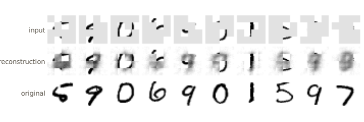
With only four of sixteen patches visible, the network does better than the obvious baseline of pasting in the average digit, but not by a wide margin, and figure 4 shows what that means. Where the visible fragments pin the digit down, the fill is a recognizable, blurred version of it; where they do not, the network paints a gray average of the candidates. The squared error rewards the average of all plausible completions, which is why the fills look soft; the same effect makes VAE samples blurry below.
Reconstruction is not the goal, though; the encoder’s representation is. The standard way to measure it is a linear probe: freeze the encoder, feed it the complete test images, average its output tokens into one 64-dimensional feature vector, and train only a linear softmax classifier on those features. We compare the trained encoder with an untrained one of the same architecture and with a linear classifier on the raw pixels.
def mae_features(model, X_in):
    with torch.no_grad():
        return model.encode(patchify(X_in)).mean(1)            # all 16 patches, averaged tokens

def linear_probe(F_train, F_test, steps=200):
    """Softmax regression on standardized features; returns test accuracy."""
    mu, sd = F_train.mean(0), F_train.std(0) + 1e-6
    F_train, F_test = (F_train - mu) / sd, (F_test - mu) / sd
    torch.manual_seed(0)
    clf = nn.Linear(F_train.shape[1], 10)
    opt = torch.optim.Adam(clf.parameters(), lr=1e-2)
    for _ in range(steps):
        loss = F.cross_entropy(clf(F_train), y)
        opt.zero_grad()
        loss.backward()
        opt.step()
    with torch.no_grad():
        return (clf(F_test).argmax(1) == y_test).float().mean().item()

torch.manual_seed(5)
untrained = MAE()                                              # same initialization as mae had
print(f"linear probe, MAE encoder:        "
      f"{linear_probe(mae_features(mae, X), mae_features(mae, X_test)):.3f}")
print(f"linear probe, untrained encoder:  "
      f"{linear_probe(mae_features(untrained, X), mae_features(untrained, X_test)):.3f}")
print(f"linear classifier on raw pixels:  {linear_probe(X, X_test):.3f}")
linear probe, MAE encoder:        0.717
linear probe, untrained encoder:  0.575
linear classifier on raw pixels:  0.857
Pre-training moves the probe accuracy well above that of the random encoder, so the encoder has learned something about digit identity from reconstruction alone, without labels. It does not beat a linear classifier on the 784 raw pixels, which on MNIST is a strong baseline; our encoder has 64 features, saw 6,000 images for ten epochs, and was never fine-tuned. The published MAE results come from large vision transformers pre-trained for hundreds of epochs on large natural-image collections and then fine-tuned. The recipe is what carries over, and nothing in it is specific to images: masking and reconstruction apply to any data that can be cut into tokens.
Variational autoencoders
The deterministic autoencoders learn codes but give no way to generate new data. The latent-variable model of module 16 does the opposite. It draws a code from a fixed prior and passes it through a network \(\mathbf{g}(\mathbf{z}, \mathbf{w})\) that gives the parameters of a distribution over data,
\[p(\mathbf{z}) = \mathcal{N}(\mathbf{z} \mid \mathbf{0}, \mathbf{I}), \qquad p(\mathbf{x} \mid \mathbf{w}) = \int p(\mathbf{x} \mid \mathbf{z}, \mathbf{w})\,p(\mathbf{z})\,d\mathbf{z},\]with \(\mathbf{z}\) of dimension \(M\). Sampling is one forward pass, but the likelihood is an integral through a neural network with no closed form, and module 16 showed that estimating it by averaging over prior samples needs more and more samples as the output noise shrinks. The variational autoencoder (Kingma and Welling, 2013; Rezende, Mohamed, and Wierstra, 2014) trains this model anyway, with three ideas:
- maximize the evidence lower bound (ELBO) instead of the likelihood, as in the EM algorithm;
- amortized inference: a second network, the encoder, approximates the posterior over \(\mathbf{z}\) for every data point in one forward pass;
- the reparameterization trick, which makes the bound differentiable with respect to the encoder’s parameters.
The evidence lower bound
For any distribution \(q(\mathbf{z})\) over the latent space, module 15 and module 16 derived the decomposition
\[\ln p(\mathbf{x} \mid \mathbf{w}) = \mathcal{L}(q, \mathbf{w}) + \mathrm{KL}\left(q(\mathbf{z}) \Vert p(\mathbf{z} \mid \mathbf{x}, \mathbf{w})\right), \qquad \mathcal{L}(q, \mathbf{w}) = \int q(\mathbf{z})\ln\frac{p(\mathbf{x} \mid \mathbf{z}, \mathbf{w})\,p(\mathbf{z})}{q(\mathbf{z})}\,d\mathbf{z} .\](In one line: \(\ln p(\mathbf{x} \mid \mathbf{w}) = \ln p(\mathbf{x}, \mathbf{z} \mid \mathbf{w}) - \ln p(\mathbf{z} \mid \mathbf{x}, \mathbf{w})\) for every \(\mathbf{z}\); add and subtract \(\ln q(\mathbf{z})\) and average over \(q\).) The KL divergence is nonnegative, so \(\mathcal{L}\) is a lower bound on the log likelihood, tight exactly when \(q\) is the true posterior. For a data set of \(N\) independent points, each point gets its own latent variable \(\mathbf{z}_n\) and its own distribution \(q_n\), and
\[\ln p(\mathcal{D} \mid \mathbf{w}) = \sum_{n=1}^{N} \mathcal{L}_n + \sum_{n=1}^{N}\mathrm{KL}\left(q_n(\mathbf{z}_n) \Vert p(\mathbf{z}_n \mid \mathbf{x}_n, \mathbf{w})\right), \qquad \mathcal{L}_n = \int q_n(\mathbf{z}_n)\ln\frac{p(\mathbf{x}_n \mid \mathbf{z}_n, \mathbf{w})\,p(\mathbf{z}_n)}{q_n(\mathbf{z}_n)}\,d\mathbf{z}_n .\]For Gaussian mixtures and probabilistic PCA the E step sets each \(q_n\) to the exact posterior, which closes the gap. Here the posterior is \(p(\mathbf{z}_n \mid \mathbf{x}_n, \mathbf{w}) = p(\mathbf{x}_n \mid \mathbf{z}_n, \mathbf{w})p(\mathbf{z}_n)/p(\mathbf{x}_n \mid \mathbf{w})\): the numerator is one pass through the decoder, but the denominator is the intractable likelihood itself. So we restrict \(q\) to a tractable family, Gaussians, and accept a gap. Maximizing \(\mathcal{L}\) over \(q\) is the same as minimizing \(\mathrm{KL}(q \Vert p)\), the reverse direction that module 02 showed tends to lock onto a single mode. Intro to ML, module 10 develops variational inference in general.
How big can the gap be? A one-dimensional example makes it concrete. Take \(z \sim \mathcal{N}(0, 1)\) and a decoder that squares the latent, \(x \mid z \sim \mathcal{N}(z^2, s^2)\) with \(s = 0.25\). For an observation \(x^\star = 2\), the latent could be near \(+\sqrt{2}\) or near \(-\sqrt{2}\), so the posterior has two equal modes. We compute \(\ln p(x^\star)\) by quadrature and find the best Gaussian \(q = \mathcal{N}(\mu, \varsigma^2)\) by grid search, using the closed-form ELBO: with \(\mathbb{E}_q[z^2] = \mu^2 + \varsigma^2\) and \(\mathbb{E}_q[z^4] = \mu^4 + 6\mu^2\varsigma^2 + 3\varsigma^4\), every term of \(\mathcal{L}\) is a polynomial expectation or the Gaussian entropy \(\frac{1}{2}\ln(2\pi e \varsigma^2)\).
s_dec, x_star = 0.25, 2.0

def log_joint(z):
    """ln p(x* | z) + ln p(z) for the squaring decoder."""
    return (-0.5 * ((x_star - z ** 2) / s_dec) ** 2 - np.log(s_dec * np.sqrt(2 * np.pi))
            - 0.5 * z ** 2 - 0.5 * np.log(2 * np.pi))

z_grid = np.linspace(-6, 6, 24001)
lj = log_joint(z_grid)
log_px = np.log(np.sum(np.exp(lj - lj.max())) * (z_grid[1] - z_grid[0])) + lj.max()
post = np.exp(lj - log_px)                                 # exact posterior on the grid
print(f"ln p(x*) by quadrature: {log_px:.4f};  posterior modes at z = "
      f"{z_grid[np.argmax(post * (z_grid < 0))]:.3f} and {z_grid[np.argmax(post * (z_grid > 0))]:.3f}")

def elbo_1d(mu, vs):
    """Closed-form ELBO for q = N(mu, vs) (vs is the variance), using Gaussian moments."""
    Ez2 = mu ** 2 + vs
    Ez4 = mu ** 4 + 6 * mu ** 2 * vs + 3 * vs ** 2
    E_sq = x_star ** 2 - 2 * x_star * Ez2 + Ez4                # E_q[(x* - z^2)^2]
    E_loglik = -0.5 * E_sq / s_dec ** 2 - np.log(s_dec * np.sqrt(2 * np.pi))
    E_logprior = -0.5 * Ez2 - 0.5 * np.log(2 * np.pi)
    entropy = 0.5 * np.log(2 * np.pi * np.e * vs)
    return E_loglik + E_logprior + entropy

mu_g, sd_g = np.meshgrid(np.linspace(-3, 3, 1201), np.linspace(0.005, 2, 800), indexing="ij")
L = elbo_1d(mu_g, sd_g ** 2)
i, j = np.unravel_index(np.argmax(L), L.shape)
print(f"best Gaussian q: mu = {mu_g[i, j]:.3f}, std = {sd_g[i, j]:.3f}, ELBO = {L[i, j]:.4f}")
print(f"gap = KL(q || posterior) = {log_px - L[i, j]:.4f}   (ln 2 = {np.log(2):.4f})")
ln p(x*) by quadrature: -2.2436;  posterior modes at z = -1.403 and 1.403
best Gaussian q: mu = -1.395, std = 0.090, ELBO = -2.9399
gap = KL(q || posterior) = 0.6964   (ln 2 = 0.6931)
The best Gaussian sits on one of the two modes (the mirror-image solution is equally good) and ignores the other, and the gap is close to \(\ln 2\): a Gaussian that covers half of a two-mode posterior loses about \(\ln 2\) nats, as Exercise 5 asks you to show. With a single mode the gap would come only from the shape mismatch. In a VAE the same thing happens at every data point, and the bound stays below the likelihood by the sum of such gaps.
Amortized inference
Fitting a separate \(q_n\) to every training point, and refitting all of them after every change to \(\mathbf{w}\), would be very slow. Instead, a VAE trains one network, the encoder (or inference network) with parameters \(\boldsymbol{\phi}\), that takes \(\mathbf{x}\) and outputs the parameters of its approximate posterior \(q(\mathbf{z} \mid \mathbf{x}, \boldsymbol{\phi})\). The cost of inference is paid once, during training, and then spread over every future data point, which is why it is called amortized inference. The usual choice is a Gaussian with diagonal covariance,
\[q(\mathbf{z} \mid \mathbf{x}, \boldsymbol{\phi}) = \prod_{j=1}^{M}\mathcal{N}\left(z_j \mid \mu_j(\mathbf{x}, \boldsymbol{\phi}), \sigma_j^2(\mathbf{x}, \boldsymbol{\phi})\right).\]The means can be any real numbers, so their output units are linear. The variances must be positive; we let the network output \(\ln\sigma_j^2\) with a linear unit and exponentiate, which is the same as an exponential activation on \(\sigma_j^2\) and keeps the gradients well scaled.
The model now has two networks with separate parameters trained on one objective: the encoder \(q(\mathbf{z} \mid \mathbf{x}, \boldsymbol{\phi})\) maps data to a distribution over codes, and the generative network \(p(\mathbf{x} \mid \mathbf{z}, \mathbf{w})\) maps codes back to a distribution over data, so it plays the role of the decoder. The structure mirrors a deterministic autoencoder, with distributions in place of points. By Bayes’ theorem, the encoder is trying to be the probabilistic inverse of the decoder.
Both parameter sets are updated together by stochastic gradient ascent on \(\sum_n \mathcal{L}_n(\mathbf{w}, \boldsymbol{\phi})\). It helps to think of it as a softened EM. An update of \(\boldsymbol{\phi}\) with \(\mathbf{w}\) fixed raises the bound toward \(\ln p(\mathbf{x} \mid \mathbf{w})\), like an E step; an update of \(\mathbf{w}\) with \(\boldsymbol{\phi}\) fixed raises the bound by improving the model, like an M step. The difference is that the “E step” never closes the gap. The true posterior need not be a diagonal Gaussian (the example above), a finite encoder cannot represent the best Gaussian for every \(\mathbf{x}\) exactly (the part of the gap due to sharing one network across all points is called the amortization gap), and stochastic training only approximately optimizes either network.
The reparameterization trick
We still have to compute the bound and its gradients. Split the ELBO for one data point into two terms by writing \(\ln\{p(\mathbf{x}_n \mid \mathbf{z}, \mathbf{w})p(\mathbf{z})/q\} = \ln p(\mathbf{x}_n \mid \mathbf{z}, \mathbf{w}) - \ln\{q/p(\mathbf{z})\}\):
\[\mathcal{L}_n(\mathbf{w}, \boldsymbol{\phi}) = \underbrace{\int q(\mathbf{z} \mid \mathbf{x}_n, \boldsymbol{\phi})\ln p(\mathbf{x}_n \mid \mathbf{z}, \mathbf{w})\,d\mathbf{z}}_{\text{expected reconstruction}} - \underbrace{\mathrm{KL}\left(q(\mathbf{z} \mid \mathbf{x}_n, \boldsymbol{\phi}) \Vert p(\mathbf{z})\right)}_{\text{stay close to the prior}} .\]The first term rewards codes from which the decoder can reconstruct \(\mathbf{x}_n\); it is the probabilistic version of the reconstruction error. The second pulls each approximate posterior toward the prior, which keeps the codes of the whole data set in the region where we will later sample.
The KL term in closed form. For one coordinate, with \(q = \mathcal{N}(\mu, \sigma^2)\) and \(p = \mathcal{N}(0, 1)\),
\[\mathrm{KL}(q \Vert p) = \mathbb{E}_q\left[\ln q(z) - \ln p(z)\right] = \mathbb{E}_q\left[-\tfrac{1}{2}\ln\sigma^2 - \frac{(z - \mu)^2}{2\sigma^2} + \frac{z^2}{2}\right] = -\tfrac{1}{2}\ln\sigma^2 - \tfrac{1}{2} + \tfrac{1}{2}(\mu^2 + \sigma^2),\]using \(\mathbb{E}_q[(z - \mu)^2] = \sigma^2\) and \(\mathbb{E}_q[z^2] = \mu^2 + \sigma^2\) (the \(\ln 2\pi\) terms cancel). A diagonal Gaussian’s KL is the sum over coordinates:
\[\mathrm{KL}\left(q(\mathbf{z} \mid \mathbf{x}_n, \boldsymbol{\phi}) \Vert p(\mathbf{z})\right) = \frac{1}{2}\sum_{j=1}^{M}\left(\mu_j^2 + \sigma_j^2 - 1 - \ln\sigma_j^2\right).\]This is the general Gaussian KL of module 03 with a standard normal as the second argument. Each summand is nonnegative and zero only at \(\mu_j = 0, \sigma_j = 1\). We check it against a Monte Carlo average of \(\ln q - \ln p\) and against PyTorch’s kl_divergence:
def gauss_kl(mu, log_var):
    """KL( N(mu, diag exp(log_var)) || N(0, I) ), summed over the last dimension."""
    return 0.5 * (mu.pow(2) + log_var.exp() - 1.0 - log_var).sum(-1)

def log_normal(z, mu, log_var):
    """ln N(z | mu, diag exp(log_var)), summed over the last dimension."""
    return (-0.5 * (z - mu).pow(2) / log_var.exp() - 0.5 * log_var
            - 0.5 * math.log(2 * math.pi)).sum(-1)

mu_q = torch.tensor(rng.normal(size=3), dtype=torch.float32)
log_var_q = torch.tensor(rng.normal(scale=0.5, size=3), dtype=torch.float32)
torch.manual_seed(12)
z = mu_q + torch.exp(0.5 * log_var_q) * torch.randn(200_000, 3)
zeros = torch.zeros(3)
mc = log_normal(z, mu_q, log_var_q) - log_normal(z, zeros, zeros)
lib = torch.distributions.kl_divergence(torch.distributions.Normal(mu_q, torch.exp(0.5 * log_var_q)),
                                        torch.distributions.Normal(0.0, 1.0)).sum()
print(f"closed form {gauss_kl(mu_q, log_var_q):.4f}   Monte Carlo {mc.mean():.4f} "
      f"(+/- {mc.std() / math.sqrt(len(mc)):.4f})   torch.distributions {lib:.4f}")
closed form 0.8070 Monte Carlo 0.8124 (+/- 0.0030) torch.distributions 0.8070
Watch out. Sign conventions for this term vary between texts. The quantity \(\frac{1}{2}\sum_j(1 + \ln\sigma_j^2 - \mu_j^2 - \sigma_j^2)\) is minus the KL divergence; it is what gets added to the expected reconstruction to form the ELBO. When you implement a VAE, write the KL as the nonnegative quantity above and subtract it, and check that your printed KL values are never negative.
The reconstruction term and its gradient. The expected reconstruction is an integral through the decoder network with no closed form, so we estimate it by sampling. With \(L\) samples from the encoder,
\[\int q(\mathbf{z} \mid \mathbf{x}_n, \boldsymbol{\phi})\ln p(\mathbf{x}_n \mid \mathbf{z}, \mathbf{w})\,d\mathbf{z} \approx \frac{1}{L}\sum_{l=1}^{L}\ln p(\mathbf{x}_n \mid \mathbf{z}_n^{(l)}, \mathbf{w}), \qquad \mathbf{z}_n^{(l)} \sim q(\mathbf{z} \mid \mathbf{x}_n, \boldsymbol{\phi}) .\]The gradient with respect to \(\mathbf{w}\) is fine: differentiate each term. The gradient with respect to \(\boldsymbol{\phi}\) is the problem. The parameters \(\boldsymbol{\phi}\) shape the distribution the samples come from, but once a sample is drawn it is just a number, with no record of how it depended on \(\boldsymbol{\phi}\). In a computational graph, the sampling step cuts the path from the loss back to the encoder.
There are two ways around it. Write the problem generically as the gradient of \(\mathbb{E}_{q_{\boldsymbol{\phi}}}[f(\mathbf{z})]\) for some function \(f\).
-
Score-function estimator (also called REINFORCE, after Williams, 1992). Move the gradient onto the density and use \(\nabla_{\boldsymbol{\phi}} q = q\,\nabla_{\boldsymbol{\phi}}\ln q\):
\[\nabla_{\boldsymbol{\phi}}\int q_{\boldsymbol{\phi}}(\mathbf{z})f(\mathbf{z})\,d\mathbf{z} = \int q_{\boldsymbol{\phi}}(\mathbf{z})\,f(\mathbf{z})\,\nabla_{\boldsymbol{\phi}}\ln q_{\boldsymbol{\phi}}(\mathbf{z})\,d\mathbf{z} \approx \frac{1}{L}\sum_{l} f(\mathbf{z}^{(l)})\,\nabla_{\boldsymbol{\phi}}\ln q_{\boldsymbol{\phi}}(\mathbf{z}^{(l)}) .\]It is unbiased and works for any \(q\), even over discrete variables, and \(f\) need not be differentiable. But it uses \(f\) only through its values, multiplied by a score that is large in the tails, so its variance is high.
-
Reparameterization. Generate the sample as a differentiable function of the parameters and of noise that does not depend on them. For a Gaussian, if \(\epsilon \sim \mathcal{N}(0, 1)\) then \(z = \mu + \sigma\epsilon\) has distribution \(\mathcal{N}(\mu, \sigma^2)\) (a linear function of a Gaussian is Gaussian with mean \(\mu\) and variance \(\sigma^2\,\mathrm{var}(\epsilon)\)). The expectation becomes one over a fixed distribution, and the gradient passes inside:
\[\nabla_{\boldsymbol{\phi}}\mathbb{E}_{\epsilon}\left[f(\boldsymbol{\mu}_{\boldsymbol{\phi}} + \boldsymbol{\sigma}_{\boldsymbol{\phi}} \odot \boldsymbol{\epsilon})\right] = \mathbb{E}_{\epsilon}\left[\nabla_{\mathbf{z}} f(\mathbf{z})^{\mathrm{T}}\,\frac{\partial \mathbf{z}}{\partial \boldsymbol{\phi}}\right], \qquad \frac{\partial z_j}{\partial \mu_j} = 1, \quad \frac{\partial z_j}{\partial \sigma_j} = \epsilon_j .\]This uses the slope of \(f\), the information of how the reconstruction changes when the code moves, which is why it needs far fewer samples. It requires a continuous \(\mathbf{z}\) and a differentiable \(f\).
A numerical comparison on a problem where we know the answer: \(q = \mathcal{N}(\mu, \sigma^2)\) with \(\mu = 0.5\), \(\sigma = 1\), and \(f(z) = (z - 2)^2\). Then \(\mathbb{E}_q[f] = (\mu - 2)^2 + \sigma^2\), so the exact gradients are \(\partial/\partial\mu = 2(\mu - 2) = -3\) and \(\partial/\partial\sigma = 2\sigma = 2\). We draw 100,000 single-sample (\(L = 1\)) estimates of each kind, letting autograd compute them: giving every sample its own copy of \(\mu\) and \(\sigma\) makes .grad hold one gradient per sample. The score-function estimator is written the way it is implemented in practice, as the gradient of a surrogate loss \(f(z)\ln q(z)\) with the sample detached. We also try it with a baseline, subtracting a constant \(b\) from \(f\) (allowed because \(\mathbb{E}_q[\nabla\ln q] = 0\)), here the natural choice \(b = \mathbb{E}_q[f]\).
def f_toy(z):
    return (z - 2.0) ** 2

mu0, sigma0, n = 0.5, 1.0, 100_000
torch.manual_seed(13)
eps = torch.randn(n)

def per_sample_grads(surrogate):
    """Gradients of surrogate(mu, sigma).sum() w.r.t. one copy of (mu, sigma) per sample."""
    mu = torch.full((n,), mu0, requires_grad=True)
    sd = torch.full((n,), sigma0, requires_grad=True)
    surrogate(mu, sd).sum().backward()
    return torch.stack([mu.grad, sd.grad], 1)

z_fixed = mu0 + sigma0 * eps                                   # the same samples, detached
b = (mu0 - 2.0) ** 2 + sigma0 ** 2                             # E_q[f], the ideal constant baseline
estimators = {
    "reparameterization": per_sample_grads(lambda mu, sd: f_toy(mu + sd * eps)),
    "score function": per_sample_grads(lambda mu, sd: f_toy(z_fixed) * log_normal(
        z_fixed[:, None], mu[:, None], 2 * torch.log(sd)[:, None])),
    "score function + baseline": per_sample_grads(lambda mu, sd: (f_toy(z_fixed) - b) * log_normal(
        z_fixed[:, None], mu[:, None], 2 * torch.log(sd)[:, None])),
}
print(f"exact gradient:              d/dmu = {2 * (mu0 - 2):6.3f}   d/dsigma = {2 * sigma0:6.3f}")
for name, g in estimators.items():
    m, s = g.mean(0), g.std(0)
    print(f"{name:26s}   mean {m[0]:6.3f} (std {s[0]:5.2f})   mean {m[1]:6.3f} (std {s[1]:5.2f})")
exact gradient:              d/dmu = -3.000   d/dsigma =  2.000
reparameterization           mean -2.993 (std  2.00)   mean  1.993 (std  4.12)
score function               mean -2.994 (std  7.18)   mean  1.995 (std 14.82)
score function + baseline    mean -3.006 (std  5.29)   mean  1.989 (std 12.12)
All three estimators are unbiased: their means agree with the exact gradient to within Monte Carlo error. Their spreads differ greatly. A single reparameterized sample has a much smaller standard deviation than a single score-function sample; the baseline helps the score-function estimator but does not close the gap. The number of samples needed for a given accuracy grows with the variance, and in a VAE the latent space has many dimensions, which makes the difference larger (Exercise 6). This is why reparameterization is sometimes described as a variance-reduction technique.
PyTorch’s distributions expose the two options as rsample(), which reparameterizes and keeps the graph, and sample(), which cuts it:
mu = torch.tensor([0.5], requires_grad=True)
q_dist = torch.distributions.Normal(mu, torch.tensor([1.0]))
print("sample():  requires_grad =", q_dist.sample().requires_grad)
print("rsample(): requires_grad =", q_dist.rsample().requires_grad)
sample():  requires_grad = False
rsample(): requires_grad = True
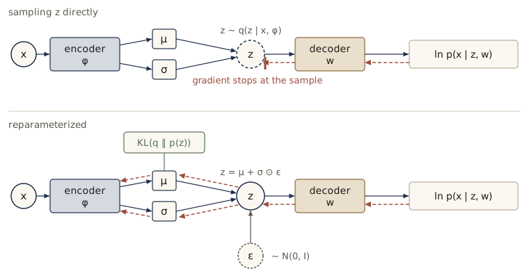
The VAE objective. Putting the pieces together, with \(L\) samples per data point and \(\mathbf{z}_n^{(l)} = \boldsymbol{\mu}_n + \boldsymbol{\sigma}_n \odot \boldsymbol{\epsilon}^{(l)}\), where \(\boldsymbol{\mu}_n = \boldsymbol{\mu}(\mathbf{x}_n, \boldsymbol{\phi})\) and \(\boldsymbol{\sigma}_n = \boldsymbol{\sigma}(\mathbf{x}_n, \boldsymbol{\phi})\),
\[\mathcal{L}(\mathbf{w}, \boldsymbol{\phi}) \approx \sum_{n}\left\{ \frac{1}{L}\sum_{l=1}^{L}\ln p(\mathbf{x}_n \mid \mathbf{z}_n^{(l)}, \mathbf{w}) - \frac{1}{2}\sum_{j=1}^{M}\left(\mu_{nj}^2 + \sigma_{nj}^2 - 1 - \ln\sigma_{nj}^2\right) \right\},\]summed over a mini-batch. In practice \(L = 1\): one sample gives a noisy estimate of the bound, but the mini-batch gradient is noisy anyway, and more updates beat more accurate ones. A training step is: run the encoder to get \(\boldsymbol{\mu}_n\) and \(\ln\boldsymbol{\sigma}_n^2\) for each image of the batch; draw \(\boldsymbol{\epsilon}\) and form \(\mathbf{z}_n\); run the decoder; evaluate the bound; backpropagate into both networks; take an optimizer step. Bishop & Bishop’s Algorithm 19.1 lists these steps.
In practice. A trained VAE is used in two ways. To generate, discard the encoder, draw \(\mathbf{z} \sim \mathcal{N}(\mathbf{0}, \mathbf{I})\), and decode. To evaluate a new point \(\widehat{\mathbf{x}}\), the ELBO is the usual stand-in for the intractable \(\ln p(\widehat{\mathbf{x}})\); estimate it with samples from the encoder \(q(\mathbf{z} \mid \widehat{\mathbf{x}}, \boldsymbol{\phi})\), not from the prior, because the encoder puts the samples where \(p(\widehat{\mathbf{x}} \mid \mathbf{z})\) is large.
A VAE for MNIST
For the likelihood \(p(\mathbf{x} \mid \mathbf{z}, \mathbf{w})\) we binarize the digits (pixel on if its intensity exceeds 0.5) and use independent Bernoulli pixels whose probabilities are the sigmoid of the decoder’s outputs, as in module 16’s treatment of discrete data. Then \(\ln p(\mathbf{x} \mid \mathbf{z}, \mathbf{w})\) is minus the binary cross-entropy summed over the 784 pixels, which F.binary_cross_entropy_with_logits computes stably from the logits. (A Gaussian likelihood on the gray-level images would work as well; the Bernoulli choice keeps the numbers comparable with the VAE literature on binarized MNIST, though our subset and our binarization are not the standard benchmark.) Encoder and decoder each have one hidden layer of 256 ReLU units.
Xb = (X > 0.5).float()                                      # binarized digits
Xb_test = (X_test > 0.5).float()

class VAE(nn.Module):
    def __init__(self, M, H=256):
        super().__init__()
        self.encoder = nn.Sequential(nn.Linear(D, H), nn.ReLU(), nn.Linear(H, 2 * M))  # mu, ln sigma^2
        self.decoder = nn.Sequential(nn.Linear(M, H), nn.ReLU(), nn.Linear(H, D))      # pixel logits

    def encode(self, x):
        mu, log_var = self.encoder(x).chunk(2, dim=-1)
        return mu, log_var

def elbo_terms(vae, x):
    """Single-sample (L = 1) expected reconstruction and closed-form KL, one value per image."""
    mu, log_var = vae.encode(x)
    z = mu + torch.exp(0.5 * log_var) * torch.randn_like(mu)          # reparameterization
    log_px = -F.binary_cross_entropy_with_logits(vae.decoder(z), x, reduction="none").sum(-1)
    return log_px, gauss_kl(mu, log_var)

def vae_loss(vae):
    def loss_fn(xb):
        log_px, kl = elbo_terms(vae, xb)
        return (kl - log_px).mean()                                   # minus the ELBO per image
    return loss_fn

def evaluate_vae(vae, X_eval, seed=0):
    torch.manual_seed(seed)
    with torch.no_grad():
        log_px, kl = elbo_terms(vae, X_eval)
    return (log_px - kl).mean().item(), log_px.mean().item(), kl.mean().item()

torch.manual_seed(22)
vae2 = VAE(2)
fit(vae_loss(vae2), vae2.parameters(), Xb, epochs=15, seed=32, report=(1, 5, 10, 15))
elbo, rec, kl = evaluate_vae(vae2, Xb_test)
print(f"M = 2 test: ELBO {elbo:.2f} nats = reconstruction {rec:.2f} - KL {kl:.2f}")
  epoch  1: training loss 265.402
  epoch  5: training loss 179.224
  epoch 10: training loss 168.212
  epoch 15: training loss 163.132
M = 2 test: ELBO -164.39 nats = reconstruction -159.77 - KL 4.62
The training loss is minus the ELBO in nats per image. The KL term shows how much information the codes carry about each image beyond what the prior already says; with two latent dimensions it is small, so most of an image’s detail cannot be encoded and the reconstruction term dominates. Compare the code spaces of the deterministic autoencoder and the VAE:
with torch.no_grad():
    mu_vae, log_var_vae = vae2.encode(Xb_test)
for name, Z in [("autoencoder codes", z_ae), ("VAE encoder means", mu_vae)]:
    print(f"{name:18s}: mean {Z.mean(0).numpy().round(2)}, std {Z.std(0).numpy().round(2)}")
post_std = torch.exp(0.5 * log_var_vae).mean(0)
print(f"VAE posterior std, averaged over test images: {post_std.numpy().round(3)}")
autoencoder codes : mean [-0.9  -2.02], std [2.43 2.82]
VAE encoder means : mean [ 0.45 -0.18], std [1.08 1.2 ]
VAE posterior std, averaged over test images: [0.148 0.126]
The autoencoder’s codes have whatever location and scale training happened to produce. The VAE’s encoder means are centered near zero with a spread close to one, because the KL term pulls every \(q(\mathbf{z} \mid \mathbf{x})\) toward \(\mathcal{N}(\mathbf{0}, \mathbf{I})\), and each image is encoded not as a point but as a small Gaussian cloud whose width is the posterior standard deviation. The two layouts are plotted in the top row of figure 6. The KL term acts as a regularizer on the code space, which is what makes it safe to sample from the prior.
Decoding a regular grid of latent points shows what the decoder has learned. We map evenly spaced probabilities through the inverse Gaussian CDF, so the grid covers the prior’s bulk evenly; figure 6 (bottom left) shows the result. Neighboring codes decode to similar images, and moving across the plane morphs one digit class into the next.
A two-dimensional code is a strong bottleneck. Now a VAE with \(M = 16\):
torch.manual_seed(36)
vae16 = VAE(16)
fit(vae_loss(vae16), vae16.parameters(), Xb, epochs=15, seed=46, report=(1, 5, 10, 15))
elbo, rec, kl = evaluate_vae(vae16, Xb_test)
print(f"M = 16 test: ELBO {elbo:.2f} nats = reconstruction {rec:.2f} - KL {kl:.2f}")
with torch.no_grad():
    mu16, log_var16 = vae16.encode(Xb_test)
    kl_per_dim = (0.5 * (mu16.pow(2) + log_var16.exp() - 1 - log_var16)).mean(0)
print("average KL per latent dimension:", kl_per_dim.numpy().round(2))
  epoch  1: training loss 278.630
  epoch  5: training loss 143.890
  epoch 10: training loss 118.689
  epoch 15: training loss 108.750
M = 16 test: ELBO -113.25 nats = reconstruction -91.58 - KL 21.67
average KL per latent dimension: [1.16 1.42 1.44 1.1  1.24 1.01 1.41 1.06 1.46 1.16 1.83 1.45 1.56 1.57
 1.52 1.27]
More latent dimensions buy a much better bound: the codes now carry many more nats per image, and the reconstruction term improves by more than the KL grows. The per-dimension KL shows how the information is spread. Here every dimension carries at least one nat; a dimension whose KL stays near zero has \(q(z_j \mid \mathbf{x}) \approx p(z_j)\) for every image, which means it carries no information and the decoder ignores it. Samples from this model are in figure 6 (bottom right).
How loose is the bound? The importance-sampling estimate of module 16, with the encoder as the proposal distribution, gives a tighter estimate of \(\ln p(\mathbf{x})\):
\[\ln p(\mathbf{x}) \approx \ln\frac{1}{K}\sum_{k=1}^{K}\frac{p(\mathbf{x} \mid \mathbf{z}_k, \mathbf{w})\,p(\mathbf{z}_k)}{q(\mathbf{z}_k \mid \mathbf{x}, \boldsymbol{\phi})}, \qquad \mathbf{z}_k \sim q(\mathbf{z} \mid \mathbf{x}, \boldsymbol{\phi}) .\]By Jensen’s inequality its expectation lies between the ELBO (which is the average of the log weights, the case \(K = 1\)) and \(\ln p(\mathbf{x})\), and it approaches \(\ln p(\mathbf{x})\) as \(K\) grows. We compute it for 500 test images:
def log_weights(vae, x, K):
    """ln p(x|z_k) + ln p(z_k) - ln q(z_k|x) for K encoder samples per image: (K, n_images)."""
    with torch.no_grad():
        mu, log_var = vae.encode(x)
        out = []
        for _ in range(K):
            z = mu + torch.exp(0.5 * log_var) * torch.randn_like(mu)
            log_px = -F.binary_cross_entropy_with_logits(vae.decoder(z), x, reduction="none").sum(-1)
            zeros = torch.zeros_like(z)
            out.append(log_px + log_normal(z, zeros, zeros) - log_normal(z, mu, log_var))
    return torch.stack(out)

torch.manual_seed(14)
lw = log_weights(vae16, Xb_test[:500], K=200)
print(f"ELBO (mean log weight):          {lw.mean():.2f}")
for K in [1, 10, 50, 200]:
    est = torch.logsumexp(lw[:K], 0) - math.log(K)
    print(f"importance estimate, K = {K:3d}:   {est.mean():.2f}")
ELBO (mean log weight):          -111.38
importance estimate, K =   1:   -111.19
importance estimate, K =  10:   -107.66
importance estimate, K =  50:   -106.58
importance estimate, K = 200:   -106.03
The estimates climb with \(K\) and level off a few nats above the ELBO. That difference is (up to the remaining bias of the \(K = 200\) estimate) the average \(\mathrm{KL}(q \Vert p(\mathbf{z} \mid \mathbf{x}))\) at the trained parameters: the price of the Gaussian, amortized posterior approximation. It is modest compared with the bound itself, which says the encoder does a reasonable job, but it is not zero, just as the one-dimensional example predicted.
Blurry samples, posterior collapse, and β
VAE samples are known for looking soft, and figure 6 shows it. The cause is the likelihood. The decoder outputs pixel probabilities, the mean of \(p(\mathbf{x} \mid \mathbf{z})\); when a code is compatible with several nearby images (a stroke slightly left or right), the mean averages them, exactly as squared error did for the MAE. Sampling the pixels instead of showing the means does not help, since independent Bernoulli pixels give salt-and-pepper noise rather than sharp strokes. Factorized likelihoods cannot express “this stroke is here or there”, and the objective’s pull toward the prior further limits how precisely each code can pin down its image.
Two opposite failures bracket good training (Bishop & Bishop §19.2.2):
- Posterior collapse. The encoder’s \(q(\mathbf{z} \mid \mathbf{x}, \boldsymbol{\phi})\) becomes equal to the prior for every \(\mathbf{x}\), the KL term drops to near zero, and the decoder learns to produce average-looking outputs without using the code. Reconstructions of an input look like a blurry generic digit. Collapse is most common when the decoder is powerful enough to model the data without a code (an autoregressive decoder, for example), and it often happens dimension by dimension: the per-dimension KL printed above is the diagnostic.
- An uncompressed code. The KL term is large, reconstructions are excellent, but the encoder’s clouds do not cover the prior, so codes drawn from \(\mathcal{N}(\mathbf{0}, \mathbf{I})\) land in regions no training image was mapped to and decode to nonsense. This is the deterministic autoencoder’s problem returning.
A single knob trades these off. The β-VAE (Higgins et al., 2017) multiplies the KL term by a coefficient \(\beta\): increasing \(\beta\) presses the codes toward the prior (better samples, worse reconstructions, and more risk of collapse), decreasing it does the opposite. A common schedule, KL annealing, starts with a small \(\beta\) and raises it during training so that the encoder learns to use the code before the KL term pushes back. Exercise 9 explores both.
Note. Many variants change one part of the recipe. For images, the encoder is usually convolutional and the decoder uses transposed convolutions (module 10). A conditional VAE feeds a label or other side information \(\mathbf{c}\) to both networks and may use a learned conditional prior \(p(\mathbf{z} \mid \mathbf{c})\), so we can ask for, say, a 7. The decoder can output a variance or the parameters of a richer distribution, such as a mixture (module 06), and the encoder can output a full covariance through a triangular factor (Exercise 7).
Summary
| Model | Constraint that prevents copying | What it gives | Key equation or property |
|---|---|---|---|
| Linear autoencoder | bottleneck of \(M < D\) linear units | the principal subspace (any basis of it) | minimum error \(\sum_{i > M}\lambda_i\); \(\mathbf{B}\mathbf{A} = \mathbf{U}_M\mathbf{U}_M^{\mathrm{T}}\) |
| Deep autoencoder | bottleneck between nonlinear layers | codes on a learned curved manifold | nonconvex; beats PCA most at small \(M\) |
| Sparse autoencoder | L1 penalty on activations | few active units per input | \(E + \lambda\sum_k \lvert z_k \rvert\) |
| Denoising autoencoder | corrupted input, clean target | robust features; the score of \(p_\sigma\) | \((\mathbf{r}(\widetilde{\mathbf{x}}) - \widetilde{\mathbf{x}})/\sigma^2 \approx \nabla\ln p_\sigma(\widetilde{\mathbf{x}})\) |
| Masked autoencoder | most patches removed; encoder sees the rest | pre-trained transformer encoder | loss on masked patches only |
| Variational autoencoder | KL to the prior; noisy codes | a generative model with an encoder | \(\mathcal{L}_n = \mathbb{E}_q[\ln p(\mathbf{x}_n \mid \mathbf{z})] - \mathrm{KL}(q \Vert p(\mathbf{z}))\) |
| Reparameterization | — | low-variance gradients through samples | \(\mathbf{z} = \boldsymbol{\mu} + \boldsymbol{\sigma}\odot\boldsymbol{\epsilon}\), \(\boldsymbol{\epsilon} \sim \mathcal{N}(\mathbf{0}, \mathbf{I})\) |
Ideas to carry forward:
- An autoencoder is only as interesting as its constraint. A bottleneck, a sparsity penalty, noise, and masking each force the network to model the data in a different way, and the linear case shows that without nonlinearity a bottleneck just rediscovers PCA.
- Denoising and density modelling are the same problem in disguise: the optimal denoiser encodes the score of the smoothed density. Diffusion models (module 20) are built on this.
- Masking plus reconstruction is a general self-supervised recipe for transformers, in language and in vision alike.
- A VAE is an autoencoder whose code is a distribution, trained on a lower bound. The encoder amortizes inference, the reparameterization trick carries gradients through the sampling step, and the gap between bound and likelihood, together with the pull toward the prior, explains both its stability and its blurry samples.
Exercises
- For the linear autoencoder, show that if \((\mathbf{A}, \mathbf{B})\) is optimal then so is \((\mathbf{G}\mathbf{A}, \mathbf{B}\mathbf{G}^{-1})\) for every invertible \(\mathbf{G}\). Then show that adding the penalty \(\lVert \mathbf{A} - \mathbf{B}^{\mathrm{T}} \rVert_F^2\) (or tying \(\mathbf{A} = \mathbf{B}^{\mathrm{T}}\)) restricts the symmetry to orthogonal \(\mathbf{G}\). Modify
linear_ae_errorto tie the weights, retrain, and check that \(\mathbf{B}^{\mathrm{T}}\mathbf{B}\) is now close to the identity. - Train the linear autoencoder with \(M = 8\) on mini-batches of the images (not on \(\mathbf{S}\)) with Adam for a few thousand steps and track the principal angles. Which angle converges slowest? Relate its speed to the gap \(\lambda_8 - \lambda_9\) printed in the notes.
- Prove that the minimizer over functions \(\mathbf{r}\) of \(\mathbb{E}\lVert \mathbf{r}(\widetilde{\mathbf{x}}) - \mathbf{x} \rVert^2\) is \(\mathbb{E}[\mathbf{x} \mid \widetilde{\mathbf{x}}]\). For data concentrated at a single point \(\mathbf{x}_0\), compute \(p_\sigma\), its score, and the optimal denoiser, and check Tweedie’s formula directly.
- Repeat the 2-D score experiment for \(\sigma \in \{0.1, 0.25, 0.5, 1.0\}\), training a fresh denoiser for each. Report the median cosine similarity between learned and true scores, measured at noisy samples and at points on a uniform grid over \([-4, 4]^2\). Where does the estimate fail, and why does it fail more for small \(\sigma\)?
- Let a posterior be an equal mixture of two Gaussians \(\mathcal{N}(\pm m, s^2)\) with \(m \gg s\). Show that the Gaussian \(q = \mathcal{N}(m, s^2)\) has \(\mathrm{KL}(q \Vert p) \to \ln 2\) as \(m/s \to \infty\). Use the 1-D squaring-decoder example to plot the ELBO gap against \(x^\star\) for \(x^\star\) from \(-1\) to \(4\), and explain the curve.
- Extend the gradient-variance experiment to \(M\) dimensions with \(f(\mathbf{z}) = \lVert \mathbf{z} - 2\cdot\mathbf{1} \rVert^2\) and \(q = \mathcal{N}(\mathbf{0.5}, \mathbf{I})\). Derive the variance of both estimators of \(\partial/\partial\mu_1\) as a function of \(M\), and confirm numerically for \(M = 1, 4, 16, 64\).
- Let \(\boldsymbol{\epsilon} \sim \mathcal{N}(\mathbf{0}, \mathbf{I})\) and \(\mathbf{z} = \boldsymbol{\mu} + \mathbf{L}\boldsymbol{\epsilon}\) with \(\mathbf{L}\) lower triangular. Show that \(\mathbf{z} \sim \mathcal{N}(\boldsymbol{\mu}, \mathbf{L}\mathbf{L}^{\mathrm{T}})\), give \(\ln\lvert \mathbf{L}\mathbf{L}^{\mathrm{T}} \rvert\) in terms of the diagonal of \(\mathbf{L}\), and write the KL to \(\mathcal{N}(\mathbf{0}, \mathbf{I})\). Describe the output layer of an encoder that produces \(\boldsymbol{\mu}\) and \(\mathbf{L}\), and say which activations keep the diagonal positive.
- Show that the ELBO can be written as \(\mathbb{E}_q[\ln p(\mathbf{x}, \mathbf{z})] + \mathrm{H}[q]\), with \(\mathrm{H}\) the entropy, and as \(\mathbb{E}_q[\ln p(\mathbf{z})] + \mathbb{E}_q[\ln\{p(\mathbf{x} \mid \mathbf{z})/q(\mathbf{z} \mid \mathbf{x})\}]\). Which form did the code use, and which form would you use if \(q\) were not Gaussian?
- Train the \(M = 16\) VAE with the KL term multiplied by \(\beta \in \{0.5, 1, 4\}\), and once with \(\beta\) rising linearly from 0 to 1 over the first 5 epochs. For each, report the test ELBO (with \(\beta = 1\)), the reconstruction term, the per-dimension KL, and the number of collapsed dimensions (KL below 0.05 nats), and compare samples by eye.
- Replace the VAE’s encoder and decoder with small convolutional networks (two strided convolutions down, two transposed convolutions up, as in module 10). Compare the test ELBO and the samples with the fully connected VAE at a similar parameter count.
- Train a denoising autoencoder with masking noise at \(\nu = 0.75\) (no patches, no transformer) and compare its linear-probe accuracy with the MAE’s. What does the MAE’s design buy, and what would change with larger images?
- In your own words: what does each of the bottleneck, the sparsity penalty, the noise, and the KL term prevent, and why does only the last one give a model you can sample from?
Going further
- Bishop & Bishop, Deep Learning: Foundations and Concepts, chapter 19 — the source for this module. Exercise 19.1 derives the score-function estimator, 19.2 and 19.3 the reparameterization for diagonal and full covariances, 19.4 the Gaussian KL term and its gradients, and 19.5–19.6 alternative forms of the ELBO.
- Diederik Kingma and Max Welling, “Auto-encoding variational Bayes”, arXiv:1312.6114, and Danilo Rezende, Shakir Mohamed, and Daan Wierstra, “Stochastic backpropagation and approximate inference in deep generative models”, arXiv:1401.4082 — the two original VAE papers. Kingma and Welling’s later monograph, “An introduction to variational autoencoders”, arXiv:1906.02691, is a thorough modern treatment.
- Pascal Vincent, Hugo Larochelle, Yoshua Bengio, and Pierre-Antoine Manzagol, “Extracting and composing robust features with denoising autoencoders”, ICML 2008; and Pascal Vincent, “A connection between score matching and denoising autoencoders”, Neural Computation, 2011.
- Kaiming He, Xinlei Chen, Saining Xie, Yanghao Li, Piotr Dollár, and Ross Girshick, “Masked autoencoders are scalable vision learners”, arXiv:2111.06377.
- Pierre Baldi and Kurt Hornik, “Neural networks and principal component analysis: learning from examples without local minima”, Neural Networks, 1989 — the linear autoencoder’s error surface.
- Related modules: representation learning in module 06; masked language models and vision transformers in module 12; the ELBO and EM in module 15; PCA and nonlinear latent-variable models in module 16; the other deep generative models in module 17, module 18, and module 20; and PCA and variational inference from Pattern Recognition and Machine Learning in Intro to ML, module 12 and Intro to ML, module 10.
These notes follow the chapters of C. M. Bishop and H. Bishop, Deep Learning: Foundations and Concepts (Springer, 2024), the course text, which the authors make free to read online. The explanations, code, figures, and exercises here are written for this course; the book remains the reference, with the full derivations and many more exercises.