CSE 676 · Module 15 · Week 11
Discrete Latent Variables
K-means, Gaussian mixtures, the EM algorithm and its relation to K-means, Bernoulli mixtures, and the evidence lower bound that justifies EM.
Companion reading: Bishop & Bishop, Deep Learning: Foundations and Concepts, chapter 15, “Discrete Latent Variables”
By the end of this module you can
- Derive the two K-means steps as exact minimizations of the distortion, explain why the algorithm stops, and seed it with k-means++.
- Use K-means to segment an image by color and as a vector quantizer on image patches, count the bits a codebook saves, and relate the codebook to the discrete latent codes of modern generative models.
- Write a Gaussian mixture as a latent-variable model with a one-hot variable, sample from it, and compute responsibilities and the log likelihood in log space.
- Explain the singularities and the label symmetry of the mixture likelihood, and show both numerically.
- Derive the EM updates for Gaussian and Bernoulli mixtures, implement them so that the log likelihood never decreases, and show that K-means is the small-variance limit of EM.
- Prove the decomposition of the log likelihood into the evidence lower bound and a KL divergence, write the bound in the three forms later modules use, and verify it at every EM iteration.
- Show that the bound touches the log likelihood with the same gradient after an E step, and explain why gradient-based training of latent-variable models is a form of generalized EM.
- Extend EM to MAP estimation, partial M steps, and incremental updates of sufficient statistics.
Contents
- K-means clustering
- Mixtures of Gaussians
- The expectation–maximization algorithm
- The evidence lower bound
- Summary
- Exercises
- Going further
In module 03 we wrote a Gaussian mixture as a weighted sum of Gaussians and fitted a small one by gradient ascent, and in module 11 we drew probabilistic models as graphs of observed and hidden variables. This module brings the two together. A mixture is what we get when a model has one hidden variable that says which component produced each observation. We never see that variable, so we call it latent, and because it takes one of \(K\) values, it is a discrete latent variable.
Latent variables are the organizing idea behind the generative models in the last part of the course. A variational autoencoder (module 19) has continuous latent variables computed by a network; a diffusion model (module 20) treats a whole chain of noisy images as latent. Both are trained by maximizing a lower bound on the log likelihood, the evidence lower bound, and that bound appears here first, in the simplest setting where every quantity can be computed exactly and checked. The discrete case also has a direct descendant in deep learning: the codebooks of vector-quantized autoencoders are learned by the same two steps as K-means.
We start with K-means clustering, which has no probabilities at all, and use it to segment a small painted image by color and to compress image patches. We then give the Gaussian mixture its latent-variable form, derive the expectation–maximization (EM) algorithm for it, and extend EM to mixtures of Bernoulli distributions on binarized MNIST digits. The last part derives EM a third time, from the evidence lower bound, and uses that view to justify MAP estimation, partial M steps, and incremental updates. The same material, with longer derivations and different examples, is in Intro to ML, module 09; here we state each result, sketch the steps, check it in code, and spend more time on the bound. Everything is NumPy, with SciPy’s logsumexp for the log-space sums and torchvision only to load MNIST.
import numpy as np
from itertools import permutations
from scipy.special import logsumexp

np.set_printoptions(precision=4, suppress=True)
rng = np.random.default_rng(15)
K-means clustering
The distortion and its two half-steps
We have \(N\) points \(\mathbf{x}_1, \dots, \mathbf{x}_N\) in \(\mathbb{R}^D\) and want to divide them into \(K\) groups, or clusters, of points that lie close together. Each cluster gets a prototype \(\boldsymbol{\mu}_k \in \mathbb{R}^D\), and each point gets binary indicators \(r_{nk} \in \{0, 1\}\) with exactly one \(r_{nk} = 1\), marking the cluster it belongs to. Writing a choice among \(K\) options as a binary vector with a single 1 is 1-of-K coding; in network code it is called a one-hot vector.
Definition. The distortion of assignments \(\{r_{nk}\}\) and prototypes \(\{\boldsymbol{\mu}_k\}\) is \(J = \sum_{n=1}^{N} \sum_{k=1}^{K} r_{nk} \lVert \mathbf{x}_n - \boldsymbol{\mu}_k \rVert^2\), the total squared distance from each point to the prototype of its cluster. K-means looks for assignments and prototypes with small \(J\).
Minimizing \(J\) jointly is a hard combinatorial problem (\(K^N\) possible assignments), but each half of it is easy when the other half is held fixed.
With the prototypes fixed, \(J\) is a sum of separate terms, one per point, and each term is smallest when its single 1 sits at the nearest prototype:
\[r_{nk} = \begin{cases} 1 & \text{if } k = \arg\min_j \lVert \mathbf{x}_n - \boldsymbol{\mu}_j \rVert^2, \\ 0 & \text{otherwise.} \end{cases}\]With the assignments fixed, \(J\) is a convex quadratic in each \(\boldsymbol{\mu}_k\). Its gradient is \(-2 \sum_n r_{nk} (\mathbf{x}_n - \boldsymbol{\mu}_k)\), and setting it to zero gives
\[\boldsymbol{\mu}_k = \frac{\sum_n r_{nk} \mathbf{x}_n}{\sum_n r_{nk}},\]the mean of the points in cluster \(k\), which is where the name comes from. Alternating exact minimizations over blocks of variables is coordinate descent. We call the assignment update the E step and the prototype update the M step, names that will make sense once we meet EM.
Each half-step can only lower \(J\) or leave it unchanged. There are finitely many assignments, and each one fixes the prototypes of the following M step, so an assignment cannot recur once \(J\) has dropped below its value: the algorithm must stop after finitely many iterations, when the assignments no longer change. The stopping point is a local minimum in the sense that neither half-step can improve it; it need not be the global minimum.
Running K-means
Our running example for the first half of the module is a two-dimensional data set of 500 points drawn from three Gaussian clusters of different shapes: a large tilted ellipse, a small round cluster, and a flat one. We keep the labels that generated each point, but only to check the results.
def make_three_clusters(N, rng):
    """N points from three 2-D Gaussians of different shapes; also returns the labels."""
    pi_true = np.array([0.5, 0.3, 0.2])
    mu_true = np.array([[-1.0, -0.5], [2.5, 2.0], [2.2, -1.8]])
    Sigma_true = np.array([[[1.6, 1.1], [1.1, 1.0]],      # long and tilted
                           [[0.25, 0.0], [0.0, 0.25]],    # small and round
                           [[0.6, -0.1], [-0.1, 0.12]]])  # flat
    z = rng.choice(3, size=N, p=pi_true)                  # which cluster made each point
    L = np.linalg.cholesky(Sigma_true)
    X = mu_true[z] + np.einsum("nij,nj->ni", L[z], rng.standard_normal((N, 2)))
    return X, z, (pi_true, mu_true, Sigma_true)

X, z_true, theta_true = make_three_clusters(500, rng)
N, D = X.shape
print("X:", X.shape, "  points per cluster:", np.bincount(z_true))
X: (500, 2) points per cluster: [237 164 99]
The implementation follows the two updates. The squared distances for all pairs come from expanding \(\lVert \mathbf{x} - \boldsymbol{\mu} \rVert^2 = \lVert \mathbf{x} \rVert^2 - 2 \mathbf{x}^{\mathrm{T}} \boldsymbol{\mu} + \lVert \boldsymbol{\mu} \rVert^2\), which needs one matrix product instead of an \(N \times K \times D\) array; that matters for the image patches later. The M step sums the points of each cluster with np.bincount. The assignments are stored as integer indices rather than one-hot rows.
def sq_dists(X, mu):
    """(N, K) squared distances ||x_n - mu_k||^2, expanded to avoid an (N, K, D) array."""
    d2 = (X ** 2).sum(1)[:, None] - 2 * X @ mu.T + (mu ** 2).sum(1)[None, :]
    return np.maximum(d2, 0.0)

def kmeans_e_step(X, mu):
    return sq_dists(X, mu).argmin(axis=1)             # r_nk = 1 for the nearest mu_k

def kmeans_m_step(X, r, mu_old):
    """Each prototype moves to the mean of its points; an empty cluster keeps its old one."""
    K = len(mu_old)
    counts = np.bincount(r, minlength=K)
    sums = np.stack([np.bincount(r, weights=X[:, d], minlength=K)
                     for d in range(X.shape[1])], axis=1)
    return np.where(counts[:, None] > 0, sums / np.maximum(counts, 1)[:, None], mu_old)

def distortion(X, r, mu):
    return ((X - mu[r]) ** 2).sum()                    # J with r stored as indices

def kmeans(X, mu, max_iter=100):
    """Batch K-means from initial prototypes mu; J is recorded after every half-step."""
    J_hist, r = [], None
    for it in range(max_iter):
        r_new = kmeans_e_step(X, mu)
        J_hist.append(distortion(X, r_new, mu))
        if r is not None and np.array_equal(r_new, r):
            break                                     # assignments unchanged: stop
        r = r_new
        mu = kmeans_m_step(X, r, mu)
        J_hist.append(distortion(X, r, mu))
    return mu, r, J_hist
We start all three prototypes above the data, a deliberately poor choice, so that the algorithm has work to do. To compare clusters with the generating labels we must allow for relabeling (cluster 0 of K-means may be cluster 2 of the data), so best_match tries all \(K!\) label permutations.
mu_start = np.array([[-3.0, 3.0], [0.0, 3.5], [3.5, 3.0]])   # all three above the data
mu_km, r_km, J_km = kmeans(X, mu_start)
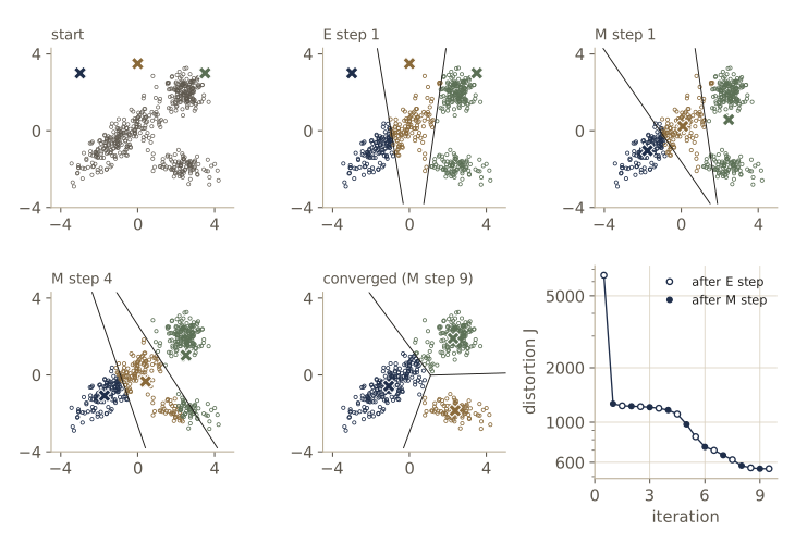
print("J after each half-step:", np.round(J_km, 1))
print("J never increases:", bool(np.all(np.diff(J_km) <= 1e-9)))
print("prototypes:\n", mu_km)

def best_match(labels, z, K):
    """Fraction of points whose cluster label agrees with z under the best relabeling."""
    return max(np.mean(np.array(p)[labels] == z) for p in permutations(range(K)))
print(f"agreement with the generating clusters: {best_match(r_km, z_true, 3):.3f}")
J after each half-step: [6506.5 1264.1 1232.2 1225.8 1219.4 1209.8 1194.2 1167.7 1110.   973.
  831.   730.8  699.7  657.   619.8  574.4  559.2  552.4  552.4]
J never increases: True
prototypes:
 [[-1.0732 -0.578 ]
 [ 2.3749 -1.8573]
 [ 2.2682  1.903 ]]
agreement with the generating clusters: 0.950
The first M step pulls the distortion from about 6500 down to about 1260, because moving the prototypes into the data is a large improvement. Then comes a long stretch of small decreases: the prototype that started on the left has captured most of the data and has to give up points slowly as the other two work their way down. After nine rounds the assignments settle at \(J \approx 552\). The clusters agree with the generating labels for 95% of the points. The mistakes are where the long tilted cluster reaches toward the flat one: K-means measures plain Euclidean distance to a center, so it prefers round clusters of similar size and cuts elongated ones at the perpendicular bisector between two prototypes.
Choosing the starting prototypes
Because K-means stops at a local minimum, the start matters. A common choice is \(K\) distinct data points picked at random. k-means++ (Arthur and Vassilvitskii, 2007) picks them one at a time instead: the first uniformly, and each later one with probability proportional to \(D(\mathbf{x})^2\), the squared distance from \(\mathbf{x}\) to the nearest prototype chosen so far. Far-away points, which are likely to lie in clusters that have no prototype yet, become likely picks. Its authors proved that the seeding alone has an expected distortion within a factor \(O(\ln K)\) of the optimum.
We compare the two seedings on nine round blobs in a three-by-three grid, a layout where K-means easily ends with two prototypes in one blob and one prototype straddling two others, and run 50 starts of each.
def kmeans_pp(X, K, rng):
    """k-means++ seeding: each new prototype is a data point drawn with prob. ~ D(x)^2."""
    idx = [rng.integers(len(X))]
    d2 = sq_dists(X, X[idx])[:, 0]                    # squared distance to nearest chosen
    for _ in range(K - 1):
        idx.append(rng.choice(len(X), p=d2 / d2.sum()))
        d2 = np.minimum(d2, sq_dists(X, X[idx[-1:]])[:, 0])
    return X[idx].copy()

grid_rng = np.random.default_rng(4)
centers = 3.0 * np.array([[i, j] for i in range(3) for j in range(3)], dtype=float)
X_grid = np.vstack([c + 0.5 * grid_rng.standard_normal((50, 2)) for c in centers])

init_rng = np.random.default_rng(0)
J_random, J_pp = [], []
for trial in range(50):
    mu0 = X_grid[init_rng.choice(len(X_grid), size=9, replace=False)]
    J_random.append(kmeans(X_grid, mu0)[2][-1])
    J_pp.append(kmeans(X_grid, kmeans_pp(X_grid, 9, init_rng))[2][-1])
J_random, J_pp = np.array(J_random), np.array(J_pp)
J_best = min(J_random.min(), J_pp.min())
for name, Js in [("random points", J_random), ("k-means++    ", J_pp)]:
    print(f"{name}: mean J {Js.mean():6.1f}, worst {Js.max():6.1f}, "
          f"runs reaching the best J ({J_best:.1f}): {np.mean(Js < J_best + 1e-6):.0%}")
random points: mean J  379.7, worst  618.6, runs reaching the best J (221.3): 26%
k-means++    : mean J  293.5, worst  597.7, runs reaching the best J (221.3): 64%
Random data points find the one-prototype-per-blob solution in about a quarter of the runs; k-means++ in about two thirds, with a clearly lower average distortion. Neither is perfect, so in practice we still run several seeded starts and keep the one with the lowest \(J\).
Sequential K-means
The batch algorithm touches all \(N\) points at every iteration. When data arrive one point at a time, we can instead update only the prototype nearest to the new point \(\mathbf{x}_n\):
\[\boldsymbol{\mu}_k^{\mathrm{new}} = \boldsymbol{\mu}_k^{\mathrm{old}} + \frac{1}{N_k} \left( \mathbf{x}_n - \boldsymbol{\mu}_k^{\mathrm{old}} \right),\]where \(N_k\) counts the points that prototype \(k\) has absorbed so far, including this one. This is the running-mean update of module 03: with step \(1/N_k\) each prototype stays exactly the mean of the points assigned to it. Replacing \(1/N_k\) by a small constant turns the running mean into an exponential moving average that forgets old points, which suits data whose distribution drifts. Intro to ML, module 09 runs the online version and compares it with the batch one.
Image segmentation and vector quantization
K-means is often applied to pixels. Treat each pixel’s color as a point in RGB space, cluster, and repaint every pixel with its prototype: the image now uses a palette of \(K\) colors. This is a crude form of image segmentation, the task of dividing an image into regions that look uniform or belong to one object; it is crude because it ignores where the pixels are.
The same idea gives a compression scheme. In lossless compression the data can be rebuilt exactly; in lossy compression we accept some error for a smaller representation. Vector quantization is lossy: store the \(K\) prototypes, now called codebook vectors, and for each data vector only the index of its nearest codebook vector. New vectors are encoded the same way. For an RGB image with 8 bits per channel, the raw pixels cost 24 bits each; the quantized image costs \(24K\) bits for the palette plus \(\lceil \log_2 K \rceil\) bits per pixel for the indices.
We need an image, so we paint one: a 96×128 still life of three balls, red, blue, and orange, in front of a wall and on a table, plus a little pixel noise. Each ball is lit from the upper left, so its color runs from a bright to a dark version of its hue, as it would in a photograph. The 12,288 pixels are our data points in \(\mathbb{R}^3\).
def make_still_life(rng, h=96, w=128):
    """Three shaded balls (red, blue, orange) before a wall, on a table; RGB in [0, 1]."""
    yy, xx = np.mgrid[0:h, 0:w].astype(float)                    # pixel row and column
    img = np.empty((h, w, 3))
    img[:] = [0.86, 0.82, 0.74] - 0.10 * (xx / w)[..., None]      # wall, darker to the right
    img[yy > 0.62 * h] = [0.52, 0.42, 0.33]                      # table top
    light = np.array([-0.5, -0.6, 0.62]) / np.linalg.norm([-0.5, -0.6, 0.62])  # upper left
    for cx, cy, r, color in [(36, 52, 21, [0.80, 0.18, 0.14]),   # red
                             (100, 50, 19, [0.20, 0.34, 0.72]),  # blue
                             (68, 64, 16, [0.92, 0.52, 0.16])]:  # orange, in front
        dx, dy = (xx - cx) / r, (yy - cy) / r
        inside = dx ** 2 + dy ** 2 < 1
        nz = np.sqrt(np.clip(1 - dx ** 2 - dy ** 2, 0, 1))       # normal (dx, dy, nz)
        cos = np.clip(dx * light[0] + dy * light[1] + nz * light[2], 0, 1)
        img[inside] = ((0.35 + 0.65 * cos)[..., None] * np.array(color))[inside]
    return np.clip(img + 0.02 * rng.standard_normal(img.shape), 0, 1)

scene = make_still_life(np.random.default_rng(7))
pixels = scene.reshape(-1, 3)                                # (N, 3): one row per pixel
palettes = {}
for K in [2, 4, 8]:
    palette, idx, J = kmeans(pixels, kmeans_pp(pixels, K, np.random.default_rng(K)))
    palettes[K] = (palette, idx)
    mse = np.mean((palette[idx] - pixels) ** 2)
    bits = 24 * K + len(pixels) * int(np.ceil(np.log2(K)))   # palette + index per pixel
    print(f"K = {K}: mean squared error {mse:.4f}, {bits / len(pixels):.3f} bits per pixel, "
          f"iterations: {len(J) // 2}")
print("the K = 4 palette (RGB):\n", palettes[4][0])
K = 2: mean squared error 0.0144, 1.004 bits per pixel, iterations: 1
K = 4: mean squared error 0.0045, 2.008 bits per pixel, iterations: 6
K = 8: mean squared error 0.0014, 3.016 bits per pixel, iterations: 16
the K = 4 palette (RGB):
 [[0.5467 0.422  0.3096]
 [0.811  0.7712 0.6914]
 [0.4999 0.1443 0.0881]
 [0.1314 0.2208 0.4685]]
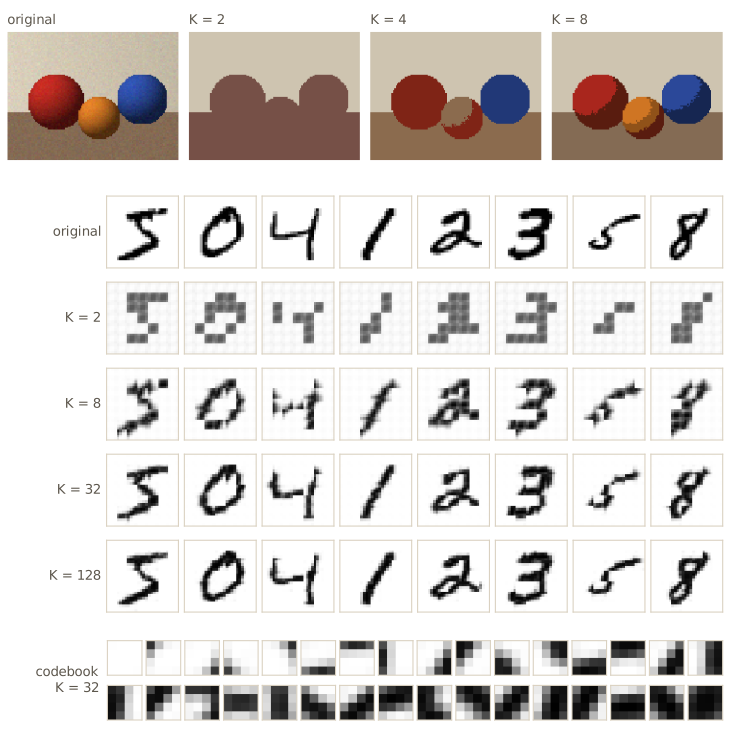
With two colors K-means separates the light wall from everything else. With four, the wall, the table, the red ball, and the blue ball get a color each, and the orange ball gets none: its lit side is painted with the table’s brown and its shaded side with the red ball’s red, whichever of the four colors is nearer. With eight, the orange ball finally gets colors of its own, but every ball is also cut into a lit part and a shaded part, and the darkest rim of the orange ball still joins the shaded red. Color clusters are not objects. Shading splits one object into several segments, and different objects of similar color are merged, because the algorithm sees only a cloud of 12,288 points in color space and nothing about where the pixels are. The compression is large, from 24 bits per pixel to about 1, 2, or 3. Bishop & Bishop §15.1.1 makes the same experiment on a photograph, and Intro to ML, module 09 on a synthetic landscape.
Single pixels throw away the correlations between neighbors, which is where most of the redundancy of real images lies. We therefore also quantize patches. On MNIST, every image is cut into 49 non-overlapping 4×4 patches, each a vector in \(\mathbb{R}^{16}\). We use the first 600 training images, which gives 29,400 patches.
from torchvision import datasets
train = datasets.MNIST(root="data", train=True, download=True)
digits = train.data[:600].float().div(255.).numpy()        # (600, 28, 28), values in [0, 1]

def to_patches(imgs, p=4):
    """Cut each image into non-overlapping p x p patches: rows of length p*p."""
    n, h, w = imgs.shape
    return imgs.reshape(n, h // p, p, w // p, p).transpose(0, 1, 3, 2, 4).reshape(-1, p * p)

def from_patches(P, n, h=28, w=28, p=4):
    return P.reshape(n, h // p, w // p, p, p).transpose(0, 1, 3, 2, 4).reshape(n, h, w)

patches = to_patches(digits)
print("patches:", patches.shape, "  round trip exact:",
      np.array_equal(from_patches(patches, len(digits)), digits))
print(f"fraction of all-zero patches: {np.mean(patches.max(axis=1) == 0):.3f}")
patches: (29400, 16)   round trip exact: True
fraction of all-zero patches: 0.631
Nearly two thirds of the patches are pure background, so one codebook vector will be spent on the empty patch. The raw gray images store 8 bits per pixel. The quantized version stores the codebook, \(16K\) numbers of 8 bits, once, plus an index of \(\lceil \log_2 K \rceil\) bits per patch:
\[\text{bits} = 8 \cdot 16 K + N_{\text{patch}} \lceil \log_2 K \rceil.\]We cap each run at 30 iterations; the distortion changes little after that.
raw_bits = digits.size * 8                                   # 8 bits per gray level
codebooks = {}
for K in [2, 8, 32, 128]:
    codebook, idx, J = kmeans(patches, kmeans_pp(patches, K, np.random.default_rng(K)),
                              max_iter=30)
    codebooks[K] = (codebook, idx)
    recon = from_patches(codebook[idx], len(digits))
    mse = np.mean((recon - digits) ** 2)
    bits = 8 * 16 * K + len(patches) * int(np.ceil(np.log2(K)))   # codebook + indices
    print(f"K = {K:3d}: {len(J) // 2:2d} iterations, mean squared error {mse:.4f}, "
          f"{bits:7d} bits = {100 * bits / raw_bits:5.2f}% of {raw_bits}")
K =   2: 10 iterations, mean squared error 0.0479,   29656 bits =  0.79% of 3763200
K =   8: 30 iterations, mean squared error 0.0243,   89224 bits =  2.37% of 3763200
K =  32: 30 iterations, mean squared error 0.0117,  151096 bits =  4.02% of 3763200
K = 128: 30 iterations, mean squared error 0.0061,  222184 bits =  5.90% of 3763200
With two codebook vectors every patch is either empty or a gray smear, and the digits become blocky silhouettes. With 32 vectors the codebook contains stroke pieces at different angles and positions, and the digits are clearly legible at 4% of the raw size. Each fourfold increase in \(K\) costs two more bits per patch and roughly halves the squared error.
Note. A vector-quantized autoencoder (VQ-VAE; van den Oord, Vinyals, and Kavukcuoglu, 2017) puts this codebook inside a network. An encoder maps an image to a grid of vectors, each vector is replaced by its nearest codebook entry (the E step), and a decoder rebuilds the image from the entries. The codebook is trained to move toward the encoder outputs assigned to it (the M step, done by gradient descent or, in a variant described in the same paper, by exponential moving averages, which is sequential K-means with a constant step). The grid of indices is a discrete latent representation, and a second model can then be trained to generate index grids.
Mixtures of Gaussians
K-means gives every point to exactly one cluster, even a point halfway between two prototypes. A probabilistic model replaces these hard assignments with probabilities.
Latent variables for the component
A Gaussian mixture has the density
\[p(\mathbf{x}) = \sum_{k=1}^{K} \pi_k \, \mathcal{N}(\mathbf{x} \mid \boldsymbol{\mu}_k, \boldsymbol{\Sigma}_k),\]with mixing coefficients \(0 \le \pi_k \le 1\), \(\sum_k \pi_k = 1\). Introduce a one-hot latent vector \(\mathbf{z} = (z_1, \dots, z_K)^{\mathrm{T}}\), with \(z_k \in \{0, 1\}\) and \(\sum_k z_k = 1\), that records which component produced \(\mathbf{x}\). Define the joint distribution by a marginal over \(\mathbf{z}\) and a conditional over \(\mathbf{x}\):
\[p(\mathbf{z}) = \prod_{k=1}^{K} \pi_k^{z_k}, \qquad p(\mathbf{x} \mid \mathbf{z}) = \prod_{k=1}^{K} \mathcal{N}(\mathbf{x} \mid \boldsymbol{\mu}_k, \boldsymbol{\Sigma}_k)^{z_k}.\]The products pick out one factor because exactly one \(z_k\) is 1, so \(p(z_k = 1) = \pi_k\) and \(p(\mathbf{x} \mid z_k = 1) = \mathcal{N}(\mathbf{x} \mid \boldsymbol{\mu}_k, \boldsymbol{\Sigma}_k)\). Summing the joint over the \(K\) states of \(\mathbf{z}\) gives back the mixture, \(p(\mathbf{x}) = \sum_{\mathbf{z}} p(\mathbf{z}) p(\mathbf{x} \mid \mathbf{z}) = \sum_k \pi_k \mathcal{N}(\mathbf{x} \mid \boldsymbol{\mu}_k, \boldsymbol{\Sigma}_k)\). As a graphical model (module 11) this is the two-node graph \(\mathbf{z} \to \mathbf{x}\), and for a data set every observation \(\mathbf{x}_n\) has its own latent \(\mathbf{z}_n\).
Nothing about the density has changed; what we gained is a joint distribution over \((\mathbf{x}, \mathbf{z})\) that is much easier to work with than the marginal. Two things follow at once.
First, ancestral sampling: draw \(\mathbf{z}\) from \(p(\mathbf{z})\), then \(\mathbf{x}\) from \(p(\mathbf{x} \mid \mathbf{z})\). That is exactly how make_three_clusters generated our data. If we keep the labels we have samples of the joint, called the complete data; if we drop them we have samples of \(p(\mathbf{x})\), the incomplete data, which is all we ever observe in practice.
Second, Bayes’ theorem gives the posterior probability that component \(k\) produced \(\mathbf{x}\):
\[\gamma(z_k) \equiv p(z_k = 1 \mid \mathbf{x}) = \frac{\pi_k \, \mathcal{N}(\mathbf{x} \mid \boldsymbol{\mu}_k, \boldsymbol{\Sigma}_k)}{\sum_{j=1}^{K} \pi_j \, \mathcal{N}(\mathbf{x} \mid \boldsymbol{\mu}_j, \boldsymbol{\Sigma}_j)}.\]\(\pi_k\) is the prior probability of component \(k\) and \(\gamma(z_k)\) is its posterior after seeing \(\mathbf{x}\). We call \(\gamma(z_k)\) the responsibility of component \(k\) for \(\mathbf{x}\), and write \(\gamma(z_{nk})\) for data point \(n\).
The code works entirely in log space, as in module 03: the numerator’s logarithm is \(\ln \pi_k + \ln \mathcal{N}(\mathbf{x}_n \mid \boldsymbol{\mu}_k, \boldsymbol{\Sigma}_k)\), the log of the denominator is a log-sum-exp over \(k\), and the Gaussian’s log density uses a Cholesky factor \(\boldsymbol{\Sigma} = \mathbf{L}\mathbf{L}^{\mathrm{T}}\) for both the quadratic form and \(\ln \lvert \boldsymbol{\Sigma} \rvert = 2 \sum_i \ln L_{ii}\).
def gauss_logpdf(X, mu, Sigma):
    """ln N(x_n | mu, Sigma) for every row of X, using a Cholesky factor Sigma = L L^T."""
    L = np.linalg.cholesky(Sigma)
    u = np.linalg.solve(L, (X - mu).T)                     # L^{-1} (x_n - mu), shape (D, N)
    half_logdet = np.log(np.diag(L)).sum()                 # (1/2) ln |Sigma|
    return -0.5 * (X.shape[1] * np.log(2 * np.pi) + (u ** 2).sum(axis=0)) - half_logdet

def log_joint(X, pi, mu, Sigma):
    """(N, K) matrix of ln p(x_n, z_nk = 1) = ln pi_k + ln N(x_n | mu_k, Sigma_k)."""
    return np.stack([np.log(pi[k]) + gauss_logpdf(X, mu[k], Sigma[k])
                     for k in range(len(pi))], axis=1)

def log_likelihood(X, pi, mu, Sigma):
    return logsumexp(log_joint(X, pi, mu, Sigma), axis=1).sum()

def responsibilities(X, pi, mu, Sigma):
    a = log_joint(X, pi, mu, Sigma)
    return np.exp(a - logsumexp(a, axis=1, keepdims=True))

gamma_true = responsibilities(X, *theta_true)
print("responsibilities of the first four points under the true parameters:\n",
      gamma_true[:4])
print("their true components:", z_true[:4])
unsure = np.mean(gamma_true.max(axis=1) < 0.9)
print(f"points whose largest responsibility is below 0.9: {unsure:.1%}")
print(f"ln p(X) under the true parameters: {log_likelihood(X, *theta_true):.2f}")
responsibilities of the first four points under the true parameters:
 [[0.0129 0.9871 0.    ]
 [0.     0.     1.    ]
 [1.     0.     0.    ]
 [0.9999 0.     0.0001]]
their true components: [1 2 0 0]
points whose largest responsibility is below 0.9: 3.6%
ln p(X) under the true parameters: -1426.42
Even with the true parameters, a point can be ambiguous: the first point came from the round cluster and gets responsibility 0.99 there and 0.01 from the tilted one. Only a few percent of the points have no component with responsibility of at least 0.9; for those the soft assignment records that the data alone cannot decide.
The likelihood function
Collect the data in the \(N \times D\) matrix \(\mathbf{X}\). For i.i.d. data the log likelihood is
\[\ln p(\mathbf{X} \mid \boldsymbol{\pi}, \boldsymbol{\mu}, \boldsymbol{\Sigma}) = \sum_{n=1}^{N} \ln \left\{ \sum_{k=1}^{K} \pi_k \, \mathcal{N}(\mathbf{x}_n \mid \boldsymbol{\mu}_k, \boldsymbol{\Sigma}_k) \right\}.\]The sum over components sits inside the logarithm, so the logarithm no longer acts on the Gaussian’s exponential, and setting derivatives to zero does not give a closed form. Before maximizing it, two properties of this function deserve attention.
Singularities. Put the mean of one component exactly on a data point, \(\boldsymbol{\mu}_j = \mathbf{x}_n\), with covariance \(\sigma_j^2 \mathbf{I}\). That point’s term contains \(\pi_j \mathcal{N}(\mathbf{x}_n \mid \mathbf{x}_n, \sigma_j^2 \mathbf{I}) = \pi_j (2\pi\sigma_j^2)^{-D/2}\), which grows without bound as \(\sigma_j \to 0\). Every other point is still covered by the remaining components, so their terms stay finite, and the log likelihood goes to \(+\infty\). A single Gaussian cannot do this: shrinking onto one point makes the density at every other point vanish, and the log likelihood goes to \(-\infty\). So the maximum likelihood problem for a mixture has no maximum at all, only these degenerate spikes and many well-behaved local maxima. We test it by adding a fourth component with weight 0.01 on the point \(\mathbf{x}_7\) to the true mixture and shrinking its width.
print("add a fourth component with weight 0.01 centered on the point x_7:")
for sigma in [1.0, 1e-2, 1e-4, 1e-8, 1e-16, 1e-64]:
    pi4 = np.append(0.99 * theta_true[0], 0.01)
    mu4 = np.vstack([theta_true[1], X[7]])
    Sigma4 = np.concatenate([theta_true[2], sigma ** 2 * np.eye(2)[None]])
    print(f"  sigma = {sigma:7.0e}:  ln p(X) = {log_likelihood(X, pi4, mu4, Sigma4):9.2f}")
print("a single Gaussian centered on x_7:")
for sigma in [1.0, 1e-2, 1e-4]:
    print(f"  sigma = {sigma:7.0e}:  ln p(X) = "
          f"{gauss_logpdf(X, X[7], sigma ** 2 * np.eye(2)).sum():14.2f}")
add a fourth component with weight 0.01 centered on the point x_7:
  sigma =   1e+00:  ln p(X) =  -1426.49
  sigma =   1e-02:  ln p(X) =  -1425.00
  sigma =   1e-04:  ln p(X) =  -1415.79
  sigma =   1e-08:  ln p(X) =  -1397.37
  sigma =   1e-16:  ln p(X) =  -1360.53
  sigma =   1e-64:  ln p(X) =  -1139.48
a single Gaussian centered on x_7:
  sigma =   1e+00:  ln p(X) =       -2478.85
  sigma =   1e-02:  ln p(X) =   -15595456.02
  sigma =   1e-04:  ln p(X) = -155991414271.39
In two dimensions the spike adds \(-2 \ln \sigma\), about 4.6 per factor of ten, so the growth is slow but unbounded: at \(\sigma = 10^{-4}\) the degenerate model already beats the true parameters, and at \(10^{-64}\) it is far ahead. The single Gaussian collapses the other way. This is overfitting in its purest form, and it is not only theoretical: EM can walk into such a spike, as we will see in the section on parameter priors, which also gives the cure.
Identifiability. Permuting the labels of the \(K\) components changes the parameter vector but not the density, so every solution comes with \(K!\) equivalent copies. A parameter is identifiable if different values give different distributions; mixture parameters are identifiable only up to this relabeling.
for perm in [(0, 1, 2), (2, 0, 1), (1, 2, 0)]:
    p = list(perm)
    ll = log_likelihood(X, theta_true[0][p], theta_true[1][p], theta_true[2][p])
    print(f"components in order {perm}: ln p(X) = {ll:.6f}")
components in order (0, 1, 2): ln p(X) = -1426.416020
components in order (2, 0, 1): ln p(X) = -1426.416020
components in order (1, 2, 0): ln p(X) = -1426.416020
For density estimation this does not matter: any of the copies is as good as any other. It does matter when we want to interpret a component (“component 2 is the round cluster”), when we average parameters across runs, and for Bayesian treatments whose posteriors have \(K!\) symmetric modes. The same symmetry appears in neural networks, where permuting hidden units leaves the function unchanged (module 06).
Maximum likelihood
We look for stationary points anyway, because they suggest an algorithm. Using \(\partial \mathcal{N}(\mathbf{x} \mid \boldsymbol{\mu}, \boldsymbol{\Sigma}) / \partial \boldsymbol{\mu} = \mathcal{N}(\mathbf{x} \mid \boldsymbol{\mu}, \boldsymbol{\Sigma}) \, \boldsymbol{\Sigma}^{-1} (\mathbf{x} - \boldsymbol{\mu})\), the derivative of the log likelihood with respect to \(\boldsymbol{\mu}_k\) is
\[\frac{\partial \ln p}{\partial \boldsymbol{\mu}_k} = \sum_{n=1}^{N} \underbrace{\frac{\pi_k \mathcal{N}(\mathbf{x}_n \mid \boldsymbol{\mu}_k, \boldsymbol{\Sigma}_k)}{\sum_j \pi_j \mathcal{N}(\mathbf{x}_n \mid \boldsymbol{\mu}_j, \boldsymbol{\Sigma}_j)}}_{\gamma(z_{nk})} \boldsymbol{\Sigma}_k^{-1} (\mathbf{x}_n - \boldsymbol{\mu}_k).\]The responsibilities appear by themselves: the gradient of a mixture is a responsibility-weighted sum of single-Gaussian gradients. Setting it to zero and multiplying by \(\boldsymbol{\Sigma}_k\) gives
\[\boldsymbol{\mu}_k = \frac{1}{N_k} \sum_{n=1}^{N} \gamma(z_{nk}) \, \mathbf{x}_n, \qquad N_k = \sum_{n=1}^{N} \gamma(z_{nk}),\]where \(N_k\) is the effective number of points of component \(k\). The same steps for \(\boldsymbol{\Sigma}_k\) reproduce the single-Gaussian covariance estimate with weights:
\[\boldsymbol{\Sigma}_k = \frac{1}{N_k} \sum_{n=1}^{N} \gamma(z_{nk}) (\mathbf{x}_n - \boldsymbol{\mu}_k)(\mathbf{x}_n - \boldsymbol{\mu}_k)^{\mathrm{T}}.\]For the mixing coefficients we add a Lagrange multiplier for \(\sum_k \pi_k = 1\) and maximize \(\ln p + \lambda (\sum_k \pi_k - 1)\). The derivative with respect to \(\pi_k\) is \(\sum_n \mathcal{N}(\mathbf{x}_n \mid \boldsymbol{\mu}_k, \boldsymbol{\Sigma}_k) / \sum_j \pi_j \mathcal{N}(\mathbf{x}_n \mid \boldsymbol{\mu}_j, \boldsymbol{\Sigma}_j) + \lambda = 0\). Multiplying by \(\pi_k\) turns the sum into \(N_k\), so \(N_k + \lambda \pi_k = 0\); summing over \(k\) gives \(\lambda = -N\), and therefore
\[\pi_k = \frac{N_k}{N}.\]These three equations are not a solution, because the responsibilities on the right depend on the parameters on the left. But they suggest a fixed-point iteration: compute the responsibilities from the current parameters (the E step, for expectation), then recompute the parameters from the responsibilities (the M step, for maximization), and repeat. That iteration is the EM algorithm for Gaussian mixtures. We will show that no iteration can lower the log likelihood; for now we check it.
def gmm_e_step(X, pi, mu, Sigma):
    """Responsibilities gamma_nk and the log likelihood, both from the same log-sum-exp."""
    a = log_joint(X, pi, mu, Sigma)
    log_px = logsumexp(a, axis=1, keepdims=True)                 # ln p(x_n)
    return np.exp(a - log_px), log_px.sum()

def gmm_m_step(X, gamma):
    N_k = gamma.sum(axis=0)                                       # effective counts
    mu = gamma.T @ X / N_k[:, None]                               # weighted means
    diff = X[None, :, :] - mu[:, None, :]                         # (K, N, D)
    Sigma = np.einsum("nk,kni,knj->kij", gamma, diff, diff) / N_k[:, None, None]
    return N_k / len(X), mu, Sigma                                # pi_k = N_k / N

def gmm_em(X, theta, max_iter=500, tol=1e-8):
    """EM from theta = (pi, mu, Sigma); returns the fit, responsibilities, ln p per iteration."""
    ll_hist = []
    for it in range(max_iter):
        gamma, ll = gmm_e_step(X, *theta)
        ll_hist.append(ll)
        if it > 0 and ll_hist[-1] - ll_hist[-2] < tol:
            break
        theta = gmm_m_step(X, gamma)
    return theta, gamma, ll_hist

K = 3
theta_start = (np.full(K, 1 / K), mu_start, np.tile(np.eye(D), (K, 1, 1)))
theta_em, gamma_em, ll_em = gmm_em(X, theta_start)
print(f"{len(ll_em)} E steps; ln p(X) at iterations 0, 1, 2, 5, 20 and at the end:")
print(np.round([ll_em[i] for i in [0, 1, 2, 5, 20, -1]], 2))
print("ln p(X) never decreases:", bool(np.all(np.diff(ll_em) >= -1e-9)))
print("mixing coefficients:", theta_em[0])
print("means:\n", theta_em[1])
print(f"agreement with the generating clusters: {best_match(gamma_em.argmax(1), z_true, 3):.3f}")
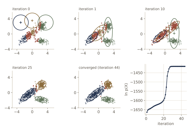
45 E steps; ln p(X) at iterations 0, 1, 2, 5, 20 and at the end:
[-4653.33 -1664.04 -1652.33 -1643.61 -1598.17 -1415.55]
ln p(X) never decreases: True
mixing coefficients: [0.4813 0.3213 0.1974]
means:
 [[-0.8318 -0.3887]
 [ 2.4684  2.0435]
 [ 2.3616 -1.8512]]
agreement with the generating clusters: 0.990
From the same poor start as K-means, with unit covariances and equal weights, EM needs 45 iterations. The log likelihood never decreases, but its progress is uneven: a slow creep from about \(-1664\) to \(-1600\) over twenty iterations, while two components share the long tilted cluster and the third straddles the other two, then a rapid climb once each component has found its own cluster. At the end the mixing coefficients and means are close to the generating ones, and the fitted covariances capture the three shapes, so the most responsible component agrees with the true label for 99% of the points, against 95% for K-means. The final log likelihood, \(-1415.55\), is higher than that of the true parameters (\(-1426.42\)), as it should be: maximum likelihood fits this sample, not the population.
EM’s iterations are more expensive than K-means’s and there are usually more of them, so a common recipe is to run K-means first and start EM from its clusters: their means, their sample covariances, and their fractions of the points.
N_k0 = np.bincount(r_km, minlength=K)
theta_km = (N_k0 / N, mu_km,
            np.array([np.cov(X[r_km == k].T, bias=True) for k in range(K)]))
theta_em2, _, ll_em2 = gmm_em(X, theta_km)
print(f"from the K-means solution: {len(ll_em2)} E steps, "
      f"ln p(X) {ll_em2[0]:.2f} -> {ll_em2[-1]:.2f}")
print("means:\n", theta_em2[1])
from the K-means solution: 20 E steps, ln p(X) -1447.15 -> -1415.55
means:
 [[-0.8318 -0.3887]
 [ 2.3616 -1.8512]
 [ 2.4684  2.0435]]
The K-means start halves the number of iterations and ends at the same log likelihood. The means are the same three vectors in a different order, because K-means happened to label the clusters differently: identifiability at work.
Watch out. EM finds a local maximum that depends on the start, and for Gaussian mixtures a component can also collapse onto a few points. In practice we run several starts (K-means or k-means++ seeded), keep the one with the highest log likelihood, and guard the covariances, for example with the prior of the section on parameter priors. The choice of \(K\) cannot be made from the training log likelihood, which keeps rising with \(K\); use held-out data (exercise 11).
The expectation–maximization algorithm
We derived EM by staring at stationarity conditions. Now we derive it again from the latent variables, which shows why it works for many models besides Gaussian mixtures.
Complete and incomplete data
Collect the observed data in \(\mathbf{X}\), the latent variables in \(\mathbf{Z}\) (for a mixture, an \(N \times K\) matrix with one-hot rows \(\mathbf{z}_n^{\mathrm{T}}\)), and all parameters in \(\boldsymbol{\theta}\). The quantity we want to maximize is the incomplete-data log likelihood
\[\ln p(\mathbf{X} \mid \boldsymbol{\theta}) = \ln \left\{ \sum_{\mathbf{Z}} p(\mathbf{X}, \mathbf{Z} \mid \boldsymbol{\theta}) \right\}.\]For continuous latent variables the sum becomes an integral; nothing below depends on the difference. The sum inside the logarithm is the source of the difficulty. Even if the joint \(p(\mathbf{X}, \mathbf{Z} \mid \boldsymbol{\theta})\) is an exponential-family distribution with a simple maximum likelihood solution, the marginal usually is not.
If someone handed us \(\mathbf{Z}\), we would maximize the complete-data log likelihood \(\ln p(\mathbf{X}, \mathbf{Z} \mid \boldsymbol{\theta})\) instead, which we assume is easy. We don’t know \(\mathbf{Z}\), but given current parameters \(\boldsymbol{\theta}^{\mathrm{old}}\) we know its posterior \(p(\mathbf{Z} \mid \mathbf{X}, \boldsymbol{\theta}^{\mathrm{old}})\). So we average the complete-data log likelihood over that posterior,
\[\mathcal{Q}(\boldsymbol{\theta}, \boldsymbol{\theta}^{\mathrm{old}}) = \sum_{\mathbf{Z}} p(\mathbf{Z} \mid \mathbf{X}, \boldsymbol{\theta}^{\mathrm{old}}) \ln p(\mathbf{X}, \mathbf{Z} \mid \boldsymbol{\theta}),\]and maximize the average. The general algorithm alternates two steps from a starting \(\boldsymbol{\theta}^{\mathrm{old}}\):
- E step. Compute the posterior \(p(\mathbf{Z} \mid \mathbf{X}, \boldsymbol{\theta}^{\mathrm{old}})\), which defines \(\mathcal{Q}(\boldsymbol{\theta}, \boldsymbol{\theta}^{\mathrm{old}})\).
- M step. Set \(\boldsymbol{\theta}^{\mathrm{new}} = \arg\max_{\boldsymbol{\theta}} \mathcal{Q}(\boldsymbol{\theta}, \boldsymbol{\theta}^{\mathrm{old}})\), then \(\boldsymbol{\theta}^{\mathrm{old}} \leftarrow \boldsymbol{\theta}^{\mathrm{new}}\), and repeat until the log likelihood stops changing.
In \(\mathcal{Q}\) the logarithm acts directly on the joint distribution, so the M step is as easy as complete-data maximum likelihood. Why averaging the log likelihood over the posterior is the right thing to do is not obvious yet; the evidence lower bound will answer that. Two extensions come almost for free. With a prior \(p(\boldsymbol{\theta})\), the M step maximizes \(\mathcal{Q}(\boldsymbol{\theta}, \boldsymbol{\theta}^{\mathrm{old}}) + \ln p(\boldsymbol{\theta})\) and EM finds MAP estimates. And the latent variables need not be modeling devices at all: they can be missing values in a data table, with EM filling in their posterior expectations. That is valid when the values are missing at random, meaning that whether a value is missing does not depend on the value itself; a sensor that fails exactly when its reading is high breaks that assumption.
Gaussian mixtures revisited
For the mixture, the complete-data likelihood is a product over points and components of the factors that the one-hot \(\mathbf{z}_n\) selects:
\[\ln p(\mathbf{X}, \mathbf{Z} \mid \boldsymbol{\mu}, \boldsymbol{\Sigma}, \boldsymbol{\pi}) = \sum_{n=1}^{N} \sum_{k=1}^{K} z_{nk} \left\{ \ln \pi_k + \ln \mathcal{N}(\mathbf{x}_n \mid \boldsymbol{\mu}_k, \boldsymbol{\Sigma}_k) \right\}.\]Compare it with the incomplete-data log likelihood: the sum over \(k\) and the logarithm have traded places. Now the logarithm meets each Gaussian directly, the problem splits into \(K\) separate single-Gaussian fits on the points assigned to each component, and the mixing coefficients are the fractions of points in each component.
For the E step we need the posterior of \(\mathbf{Z}\). By Bayes’ theorem it is proportional to the joint, \(\prod_n \prod_k [\pi_k \mathcal{N}(\mathbf{x}_n \mid \boldsymbol{\mu}_k, \boldsymbol{\Sigma}_k)]^{z_{nk}}\), which factorizes over \(n\): under the posterior the \(\mathbf{z}_n\) are independent, each with the responsibilities as its probabilities. (In the graph of module 11 this is d-separation: the \(\mathbf{z}_n\) are connected only through the parameters, which are fixed.) The complete-data log likelihood is linear in the \(z_{nk}\), and \(\mathbb{E}[z_{nk}] = \gamma(z_{nk})\), so
\[\mathcal{Q}(\boldsymbol{\theta}, \boldsymbol{\theta}^{\mathrm{old}}) = \mathbb{E}_{\mathbf{Z}}[\ln p(\mathbf{X}, \mathbf{Z} \mid \boldsymbol{\theta})] = \sum_{n=1}^{N} \sum_{k=1}^{K} \gamma(z_{nk}) \left\{ \ln \pi_k + \ln \mathcal{N}(\mathbf{x}_n \mid \boldsymbol{\mu}_k, \boldsymbol{\Sigma}_k) \right\},\]with the responsibilities computed at \(\boldsymbol{\theta}^{\mathrm{old}}\). Maximizing this is the complete-data problem with soft labels, and its solution is exactly the M step we already have. We check two things: that the M step with known one-hot labels is the complete-data fit, and that the ordinary M step maximizes \(\mathcal{Q}\) (random perturbations of its output never do better).
def expected_complete_ll(X, gamma, pi, mu, Sigma):
    """Q: sum_n sum_k gamma_nk {ln pi_k + ln N(x_n | mu_k, Sigma_k)}."""
    return np.sum(gamma * log_joint(X, pi, mu, Sigma))

Z_true = np.eye(K)[z_true]                          # one-hot rows z_n: the complete data
theta_complete = gmm_m_step(X, Z_true)              # the M step with hard, known labels
print("complete-data fit, mixing coefficients:", theta_complete[0])
print("fraction of points in each cluster:     ", np.bincount(z_true) / N)

gamma_old, _ = gmm_e_step(X, *theta_start)          # E step at the starting parameters
theta_new = gmm_m_step(X, gamma_old)                # M step
Q_new = expected_complete_ll(X, gamma_old, *theta_new)
pert_rng = np.random.default_rng(1)
worse = 0
for trial in range(200):                            # nudge the means and covariances
    mu_p = theta_new[1] + 0.05 * pert_rng.standard_normal(theta_new[1].shape)
    A = 0.05 * pert_rng.standard_normal((K, D, D))
    Sigma_p = theta_new[2] + A @ A.transpose(0, 2, 1)
    worse += expected_complete_ll(X, gamma_old, theta_new[0], mu_p, Sigma_p) < Q_new
print(f"Q at the M-step parameters: {Q_new:.3f};  perturbed parameters lower in {worse}/200")
complete-data fit, mixing coefficients: [0.474 0.328 0.198]
fraction of points in each cluster:      [0.474 0.328 0.198]
Q at the M-step parameters: -1824.341;  perturbed parameters lower in 200/200
The i.i.d. assumption is what made the posterior factorize. For ordered data such as speech or text, the latent states of neighboring observations are linked in a Markov chain, giving a hidden Markov model. EM still applies, but the E step must pass messages along the chain to get the posterior marginals; Intro to ML, module 13 derives it.
Relation to K-means
K-means makes hard assignments; EM makes soft ones. The connection is a limit. Give every component the same fixed covariance \(\epsilon \mathbf{I}\), so that only the means and mixing coefficients are learned. The responsibilities become
\[\gamma(z_{nk}) = \frac{\pi_k \exp\{-\lVert \mathbf{x}_n - \boldsymbol{\mu}_k \rVert^2 / 2\epsilon\}}{\sum_j \pi_j \exp\{-\lVert \mathbf{x}_n - \boldsymbol{\mu}_j \rVert^2 / 2\epsilon\}}.\]As \(\epsilon \to 0\) every exponential goes to zero, but the one with the smallest distance goes slowest and takes over the sum, so \(\gamma(z_{nk}) \to r_{nk}\), the K-means assignment (as long as no \(\pi_k\) is zero). The M step for the means then becomes the K-means M step, and \(\epsilon\) times the expected complete-data log likelihood tends to \(-\frac{1}{2} J\) (exercise 5). K-means is EM for this mixture in the limit of vanishing variance; it learns no covariances, which is why it prefers round clusters of similar size.
def em_shared_variance(X, mu, eps, max_iter=500, tol=1e-10):
    """EM for a mixture with every covariance fixed at eps * I; only pi and mu are learned."""
    pi = np.full(len(mu), 1 / len(mu))
    for it in range(max_iter):
        a = np.log(pi) - sq_dists(X, mu) / (2 * eps)            # ln pi_k + ln N, up to a const
        gamma = np.exp(a - logsumexp(a, axis=1, keepdims=True))
        N_k = gamma.sum(axis=0)
        mu_new, pi = gamma.T @ X / N_k[:, None], N_k / len(X)
        if np.abs(mu_new - mu).max() < tol:
            return mu_new, gamma, it + 1
        mu = mu_new
    return mu, gamma, max_iter

for eps in [1.0, 0.3, 0.1, 0.03, 0.01]:
    mu_eps, gamma_eps, iters = em_shared_variance(X, mu_start, eps)
    soft = np.sum(gamma_eps.max(axis=1) < 0.99)
    gap = np.abs(mu_eps - mu_km).max()
    print(f"eps = {eps:4.2f}: {iters:3d} iterations, points with max responsibility < 0.99: "
          f"{soft:3d}, gap to K-means {gap:.1e}")
eps = 1.00:  36 iterations, points with max responsibility < 0.99: 122, gap to K-means 3.7e-02
eps = 0.30:  28 iterations, points with max responsibility < 0.99:  28, gap to K-means 5.3e-03
eps = 0.10:  19 iterations, points with max responsibility < 0.99:   8, gap to K-means 8.2e-04
eps = 0.03:  12 iterations, points with max responsibility < 0.99:   0, gap to K-means 1.0e-06
eps = 0.01:  11 iterations, points with max responsibility < 0.99:   0, gap to K-means 1.2e-14
From the same start as K-means, the means approach the K-means prototypes as \(\epsilon\) shrinks. At \(\epsilon = 1\) over a hundred points are shared between components and the means differ by a few hundredths; at \(\epsilon = 0.03\) every responsibility is within 0.01 of 0 or 1; at \(\epsilon = 0.01\) the means equal the K-means prototypes to rounding error.
Mixtures of Bernoulli distributions
EM is not tied to Gaussians. Our next model is for binary vectors \(\mathbf{x} = (x_1, \dots, x_D)^{\mathrm{T}}\), \(x_i \in \{0, 1\}\), such as black-and-white images. A single multivariate Bernoulli distribution treats the \(D\) bits as independent:
\[p(\mathbf{x} \mid \boldsymbol{\mu}) = \prod_{i=1}^{D} \mu_i^{x_i} (1 - \mu_i)^{1 - x_i}.\]Its mean is \(\boldsymbol{\mu}\) and its covariance is \(\operatorname{diag}\{\mu_i (1 - \mu_i)\}\): it cannot say that two pixels tend to be on together. A mixture \(p(\mathbf{x} \mid \boldsymbol{\mu}, \boldsymbol{\pi}) = \sum_k \pi_k \, p(\mathbf{x} \mid \boldsymbol{\mu}_k)\) can. Its mean is \(\sum_k \pi_k \boldsymbol{\mu}_k\) and its covariance is
\[\operatorname{cov}[\mathbf{x}] = \sum_{k=1}^{K} \pi_k \left\{ \boldsymbol{\Sigma}_k + \boldsymbol{\mu}_k \boldsymbol{\mu}_k^{\mathrm{T}} \right\} - \mathbb{E}[\mathbf{x}] \mathbb{E}[\mathbf{x}]^{\mathrm{T}}, \qquad \boldsymbol{\Sigma}_k = \operatorname{diag}\{\mu_{ki}(1 - \mu_{ki})\},\]which is not diagonal: bits that are independent within each component become correlated through the shared component (exercise 6 proves the formula). This model is also called latent class analysis.
EM goes through as before. With the same one-hot latent \(\mathbf{z}_n\), the complete-data log likelihood is
\[\ln p(\mathbf{X}, \mathbf{Z} \mid \boldsymbol{\mu}, \boldsymbol{\pi}) = \sum_{n=1}^{N} \sum_{k=1}^{K} z_{nk} \left\{ \ln \pi_k + \sum_{i=1}^{D} \left[ x_{ni} \ln \mu_{ki} + (1 - x_{ni}) \ln (1 - \mu_{ki}) \right] \right\}.\]The E step computes \(\gamma(z_{nk}) = \pi_k p(\mathbf{x}_n \mid \boldsymbol{\mu}_k) / \sum_j \pi_j p(\mathbf{x}_n \mid \boldsymbol{\mu}_j)\). The M step maximizes the expectation, which replaces \(z_{nk}\) by \(\gamma(z_{nk})\). The derivative with respect to \(\mu_{ki}\) is \(\sum_n \gamma(z_{nk}) \{ x_{ni} / \mu_{ki} - (1 - x_{ni}) / (1 - \mu_{ki}) \}\); multiplying by \(\mu_{ki}(1 - \mu_{ki})\) and setting it to zero gives
\[\boldsymbol{\mu}_k = \frac{1}{N_k} \sum_{n=1}^{N} \gamma(z_{nk}) \, \mathbf{x}_n, \qquad \pi_k = \frac{N_k}{N},\]the responsibility-weighted average of the binary vectors, with \(\pi_k\) from the same Lagrange argument as before.
Note. Bernoulli mixtures have no singularities. Each \(p(\mathbf{x}_n \mid \boldsymbol{\mu}_k)\) is a probability, at most 1, so every term of the log likelihood is at most 0. The log likelihood can go to \(-\infty\) (a \(\mu_{ki}\) of exactly 0 where some image has that pixel on), and EM, which only goes uphill, will not go there from a sensible start. We still keep \(\mu_{ki}\) a hair inside \((0, 1)\) so that the logarithms of pixels that happen to be always off stay finite.
We fit a mixture of \(K = 10\) Bernoulli distributions to the first 2000 MNIST training digits, binarized at 0.5, so \(D = 784\). The labels are kept aside to inspect the result. For the log joint, one matrix product does all points and components at once, because \(\ln p(\mathbf{x} \mid \boldsymbol{\mu}_k)\) is linear in \(\mathbf{x}\).
train_X = train.data[:2000].float().div(255.).numpy().reshape(2000, -1)
X_bin = (train_X > 0.5).astype(float)                  # binarize: D = 784 pixels
y_bin = train.targets[:2000].numpy()                   # labels, used only to inspect
print("binary digits:", X_bin.shape, f"  fraction of pixels on: {X_bin.mean():.3f}")
binary digits: (2000, 784) fraction of pixels on: 0.132
We start each component halfway between the average digit and one randomly chosen digit. Bishop & Bishop start from random values in a band around 0.5, which also works; starting near data points makes it less likely that a component ends up owning almost no images.
def bernoulli_log_joint(X, pi, mu):
    """(N, K): ln pi_k + sum_i [x_ni ln mu_ki + (1 - x_ni) ln(1 - mu_ki)]."""
    return np.log(pi) + X @ np.log(mu).T + (1 - X) @ np.log1p(-mu).T

def bernoulli_em(X, mu, max_iter=100, rtol=1e-6, floor=1e-6):
    N = len(X)
    pi = np.full(len(mu), 1 / len(mu))
    ll_hist = []
    for it in range(max_iter):
        a = bernoulli_log_joint(X, pi, mu)                          # E step
        log_px = logsumexp(a, axis=1, keepdims=True)
        gamma = np.exp(a - log_px)
        ll_hist.append(log_px.sum())
        if it > 0 and ll_hist[-1] - ll_hist[-2] < rtol * abs(ll_hist[-1]):
            break
        N_k = gamma.sum(axis=0)                                     # M step
        pi = N_k / N
        mu = np.clip(gamma.T @ X / N_k[:, None], floor, 1 - floor)  # kept inside (0, 1)
    return pi, mu, gamma, ll_hist

K_b = 10
b_rng = np.random.default_rng(2)
mu_b0 = 0.5 * X_bin.mean(axis=0) + 0.5 * X_bin[b_rng.choice(len(X_bin), K_b, replace=False)]
pi_b, mu_b, gamma_b, ll_b = bernoulli_em(X_bin, np.clip(mu_b0, 0.05, 0.95))
print(f"{len(ll_b)} E steps; ln p(X) at iterations 0, 1, 5, and the end:",
      np.round([ll_b[0], ll_b[1], ll_b[5], ll_b[-1]], 1))
print("ln p(X) never decreases:", bool(np.all(np.diff(ll_b) >= -1e-6)))
mu_one = np.clip(X_bin.mean(axis=0), 1e-6, 1 - 1e-6)               # a single Bernoulli
ll_one = bernoulli_log_joint(X_bin, np.ones(1), mu_one[None]).sum()
print(f"single Bernoulli: ln p(X) = {ll_one:.1f}")
38 E steps; ln p(X) at iterations 0, 1, 5, and the end: [-431696.3 -344366.2 -328317.5 -323383. ]
ln p(X) never decreases: True
single Bernoulli: ln p(X) = -406874.8
EM converges in under 40 iterations, and the mixture’s log likelihood is about 83,000 nats higher than the single Bernoulli’s, some 42 nats per image. To see what the components learned, we list, for each component, the labels of the images for which it is most responsible.
hard = gamma_b.argmax(axis=1)
for k in np.argsort(-pi_b):
    counts = np.bincount(y_bin[hard == k], minlength=10)
    top = np.argsort(-counts)[:2]
    print(f"component {k}: pi = {pi_b[k]:.3f}, {counts.sum():3d} images, most common labels "
          f"{top[0]} ({counts[top[0]]}) and {top[1]} ({counts[top[1]]})")
purity = sum(np.bincount(y_bin[hard == k]).max() for k in range(K_b)) / len(y_bin)
print(f"images whose component's most common label is their own: {purity:.1%}")
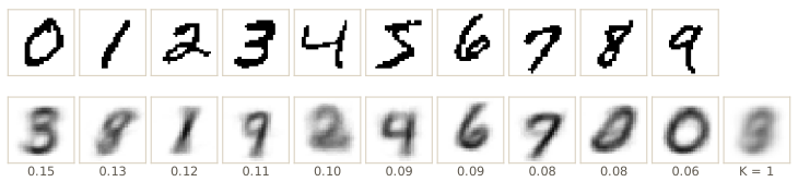
component 9: pi = 0.150, 300 images, most common labels 3 (137) and 5 (75)
component 1: pi = 0.126, 253 images, most common labels 8 (84) and 5 (69)
component 0: pi = 0.122, 243 images, most common labels 1 (206) and 2 (12)
component 7: pi = 0.110, 219 images, most common labels 9 (89) and 7 (67)
component 4: pi = 0.096, 191 images, most common labels 2 (114) and 6 (30)
component 3: pi = 0.091, 183 images, most common labels 4 (97) and 9 (51)
component 8: pi = 0.087, 175 images, most common labels 6 (158) and 0 (3)
component 6: pi = 0.079, 159 images, most common labels 7 (107) and 9 (29)
component 2: pi = 0.077, 154 images, most common labels 0 (58) and 2 (54)
component 5: pi = 0.061, 123 images, most common labels 0 (113) and 5 (7)
images whose component's most common label is their own: 58.1%
The model was never shown a label, yet several components are nearly pure digit classes: one holds mostly 1s, one mostly 6s, one mostly 0s. Others mix digits that share strokes when binarized and viewed pixel by pixel, such as 3 with 5, 4 with 9, and 7 with 9, and the 0s are split between a round and a slanted style. Overall the most common label of an image’s component is its own label for 58% of the images. Clustering finds the structure that the pixel-level model can see, which is not the same as the structure we care about; a mixture over learned features, not raw pixels, does much better.
The evidence lower bound
We now derive EM a third time, from a lower bound on the log likelihood. This bound is the central object of the rest of the course’s generative models, so we set up the notation carefully.
The decomposition
As before, \(\mathbf{X}\) is observed, \(\mathbf{Z}\) is latent (discrete here; replace sums by integrals for continuous \(\mathbf{Z}\)), and \(\boldsymbol{\theta}\) are the parameters. Take any distribution \(q(\mathbf{Z})\) over the latent variables. Then
\[\ln p(\mathbf{X} \mid \boldsymbol{\theta}) = \mathcal{L}(q, \boldsymbol{\theta}) + \mathrm{KL}(q \Vert p),\]where
\[\begin{aligned} \mathcal{L}(q, \boldsymbol{\theta}) &= \sum_{\mathbf{Z}} q(\mathbf{Z}) \ln \frac{p(\mathbf{X}, \mathbf{Z} \mid \boldsymbol{\theta})}{q(\mathbf{Z})}, \\ \mathrm{KL}(q \Vert p) &= -\sum_{\mathbf{Z}} q(\mathbf{Z}) \ln \frac{p(\mathbf{Z} \mid \mathbf{X}, \boldsymbol{\theta})}{q(\mathbf{Z})}. \end{aligned}\]To prove it, write the product rule as \(\ln p(\mathbf{X}, \mathbf{Z} \mid \boldsymbol{\theta}) = \ln p(\mathbf{Z} \mid \mathbf{X}, \boldsymbol{\theta}) + \ln p(\mathbf{X} \mid \boldsymbol{\theta})\) and substitute it into \(\mathcal{L}\):
\[\mathcal{L}(q, \boldsymbol{\theta}) = \sum_{\mathbf{Z}} q(\mathbf{Z}) \ln \frac{p(\mathbf{Z} \mid \mathbf{X}, \boldsymbol{\theta})}{q(\mathbf{Z})} + \ln p(\mathbf{X} \mid \boldsymbol{\theta}) \sum_{\mathbf{Z}} q(\mathbf{Z}) = -\mathrm{KL}(q \Vert p) + \ln p(\mathbf{X} \mid \boldsymbol{\theta}),\]using \(\sum_{\mathbf{Z}} q(\mathbf{Z}) = 1\). The second term is the Kullback–Leibler divergence (module 02) from \(q\) to the posterior over the latent variables. It is never negative and is zero exactly when \(q(\mathbf{Z}) = p(\mathbf{Z} \mid \mathbf{X}, \boldsymbol{\theta})\). Hence:
Result. For every distribution \(q\) over the latent variables,
\[\mathcal{L}(q, \boldsymbol{\theta}) \le \ln p(\mathbf{X} \mid \boldsymbol{\theta}),\]with equality if and only if \(q\) is the posterior \(p(\mathbf{Z} \mid \mathbf{X}, \boldsymbol{\theta})\). \(\mathcal{L}(q, \boldsymbol{\theta})\) is the evidence lower bound (ELBO), also called the variational lower bound, and the gap between it and the log likelihood is exactly \(\mathrm{KL}(q \Vert p)\).
The word evidence is another name for the (marginal) likelihood \(p(\mathbf{X} \mid \boldsymbol{\theta})\), from its role in Bayesian model comparison. \(\mathcal{L}\) is an ordinary function of \(\boldsymbol{\theta}\) and a functional of \(q\): it takes a whole distribution as its argument. Notice the two differences between the terms: \(\mathcal{L}\) contains the joint \(p(\mathbf{X}, \mathbf{Z} \mid \boldsymbol{\theta})\), which we can evaluate, while the KL term contains the posterior, which may be intractable; and they enter with opposite signs. The same inequality also follows from Jensen’s inequality applied to the concave logarithm, but the decomposition tells us more, because it names the gap.
For the mixture we can compute everything exactly. With a factorized \(q(\mathbf{Z}) = \prod_n q(\mathbf{z}_n)\), stored as an \(N \times K\) matrix whose rows are distributions, both terms become sums over points. We evaluate the decomposition at the EM solution for four choices of \(q\).
def elbo_terms(X, q, pi, mu, Sigma):
    """For a factorized q (row n = q(z_n)), return L(q, theta), KL(q || p(Z | X, theta)),
    and ln p(X | theta), all summed over the data points."""
    a = log_joint(X, pi, mu, Sigma)                          # ln p(x_n, z_n = k | theta)
    log_px = logsumexp(a, axis=1, keepdims=True)             # ln p(x_n | theta)
    log_post = a - log_px                                    # ln p(z_n = k | x_n, theta)
    log_q = np.log(np.maximum(q, 1e-300))                    # 0 ln 0 = 0
    L = np.sum(q * (a - log_q))                              # the ELBO
    KL = np.sum(q * (log_q - log_post))                      # the gap
    return L, KL, log_px.sum()

q_rng = np.random.default_rng(3)
q_choices = {"uniform q": np.full((N, K), 1 / K),
             "random q": q_rng.dirichlet(np.ones(K), size=N),
             "one-hot true labels": Z_true,
             "posterior q": responsibilities(X, *theta_em)}
for name, q in q_choices.items():
    L, KL, lp = elbo_terms(X, q, *theta_em)
    print(f"{name:20s} L = {L:9.2f}  KL = {round(KL, 6) + 0.0:8.2f}  "
          f"L + KL = {L + KL:9.2f}  ln p = {lp:9.2f}")
uniform q            L = -12069.03  KL = 10653.48  L + KL =  -1415.55  ln p =  -1415.55
random q             L = -12187.28  KL = 10771.73  L + KL =  -1415.55  ln p =  -1415.55
one-hot true labels  L =  -1430.12  KL =    14.56  L + KL =  -1415.55  ln p =  -1415.55
posterior q          L =  -1415.55  KL =     0.00  L + KL =  -1415.55  ln p =  -1415.55
The two terms always add up to the same log likelihood. A uniform or random \(q\) gives a very loose bound. The true labels, used as a one-hot \(q\), give a tight but not exact bound: they are right for most points but claim certainty where the posterior is unsure. Only the posterior closes the gap.
Definition. Three equivalent ways of writing the evidence lower bound, which later modules use:
\[\begin{aligned} \mathcal{L}(q, \boldsymbol{\theta}) &= \ln p(\mathbf{X} \mid \boldsymbol{\theta}) - \mathrm{KL}\big(q(\mathbf{Z}) \Vert p(\mathbf{Z} \mid \mathbf{X}, \boldsymbol{\theta})\big) \\ &= \mathbb{E}_{q}[\ln p(\mathbf{X}, \mathbf{Z} \mid \boldsymbol{\theta})] + \mathrm{H}[q] \\ &= \mathbb{E}_{q}[\ln p(\mathbf{X} \mid \mathbf{Z}, \boldsymbol{\theta})] - \mathrm{KL}\big(q(\mathbf{Z}) \Vert p(\mathbf{Z} \mid \boldsymbol{\theta})\big), \end{aligned}\]where \(\mathrm{H}[q] = -\sum_{\mathbf{Z}} q(\mathbf{Z}) \ln q(\mathbf{Z})\) is the entropy of \(q\). The first shows the gap, the second is what EM’s M step maximizes, and the third, a reconstruction term minus a KL divergence from \(q\) to the prior over the latents, is the form in which the variational autoencoder of module 19 writes its training objective.
The second form is the definition with the logarithm of a quotient split in two. The third splits the joint as \(p(\mathbf{X}, \mathbf{Z} \mid \boldsymbol{\theta}) = p(\mathbf{X} \mid \mathbf{Z}, \boldsymbol{\theta}) p(\mathbf{Z} \mid \boldsymbol{\theta})\) and collects the prior term with the entropy. For the mixture the prior is \(p(z_{nk} = 1) = \pi_k\), and we check all three numerically for the random \(q\).
q = q_choices["random q"]
a = log_joint(X, *theta_em)
log_q = np.log(q)
energy_plus_entropy = np.sum(q * a) - np.sum(q * log_q)       # E_q[ln p(X, Z)] + H[q]
log_prior = np.log(theta_em[0])                               # ln p(z_n = k) = ln pi_k
recon = np.sum(q * (a - log_prior))                           # E_q[ln p(X | Z)]
kl_prior = np.sum(q * (log_q - log_prior))                    # KL(q(Z) || p(Z))
L, _, _ = elbo_terms(X, q, *theta_em)
print(f"L                              = {L:.6f}")
print(f"E_q[ln p(X,Z)] + H[q]          = {energy_plus_entropy:.6f}")
print(f"E_q[ln p(X|Z)] - KL(q || p(Z)) = {recon - kl_prior:.6f}")
L                              = -12187.278078
E_q[ln p(X,Z)] + H[q]          = -12187.278078
E_q[ln p(X|Z)] - KL(q || p(Z)) = -12187.278078
EM revisited
EM is coordinate ascent on \(\mathcal{L}(q, \boldsymbol{\theta})\), alternating between \(q\) and \(\boldsymbol{\theta}\).
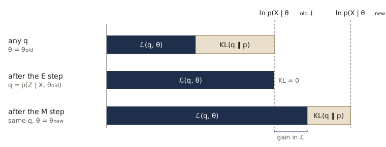
E step: maximize \(\mathcal{L}(q, \boldsymbol{\theta}^{\mathrm{old}})\) over \(q\). The sum \(\mathcal{L} + \mathrm{KL}\) is \(\ln p(\mathbf{X} \mid \boldsymbol{\theta}^{\mathrm{old}})\), which does not depend on \(q\), so maximizing \(\mathcal{L}\) means making the KL term zero: \(q(\mathbf{Z}) = p(\mathbf{Z} \mid \mathbf{X}, \boldsymbol{\theta}^{\mathrm{old}})\). Afterward the bound equals the log likelihood.
M step: maximize \(\mathcal{L}(q, \boldsymbol{\theta})\) over \(\boldsymbol{\theta}\) with \(q\) fixed. Substituting the posterior for \(q\) in the second form of the bound gives
\[\mathcal{L}(q, \boldsymbol{\theta}) = \sum_{\mathbf{Z}} p(\mathbf{Z} \mid \mathbf{X}, \boldsymbol{\theta}^{\mathrm{old}}) \ln p(\mathbf{X}, \mathbf{Z} \mid \boldsymbol{\theta}) + \mathrm{H}[q] = \mathcal{Q}(\boldsymbol{\theta}, \boldsymbol{\theta}^{\mathrm{old}}) + \text{const},\]because the entropy of \(q\) does not involve \(\boldsymbol{\theta}\). So the M step maximizes \(\mathcal{Q}\), which is where the “expected complete-data log likelihood” of the previous section comes from. \(\boldsymbol{\theta}\) appears only inside the logarithm of the joint, which is why the M step is easy whenever the joint is in the exponential family.
Why the log likelihood cannot fall. Let \(q\) be the posterior at \(\boldsymbol{\theta}^{\mathrm{old}}\). The decomposition at \(\boldsymbol{\theta}^{\mathrm{new}}\) and the zero gap at \(\boldsymbol{\theta}^{\mathrm{old}}\) give
\[\ln p(\mathbf{X} \mid \boldsymbol{\theta}^{\mathrm{new}}) - \ln p(\mathbf{X} \mid \boldsymbol{\theta}^{\mathrm{old}}) = \underbrace{\mathcal{L}(q, \boldsymbol{\theta}^{\mathrm{new}}) - \mathcal{L}(q, \boldsymbol{\theta}^{\mathrm{old}})}_{\ge 0 \text{ (M step)}} + \underbrace{\mathrm{KL}\big(q \Vert p(\mathbf{Z} \mid \mathbf{X}, \boldsymbol{\theta}^{\mathrm{new}})\big)}_{\ge 0}.\]The log likelihood rises by at least as much as the bound. It stays put only if the M step cannot improve the bound, which happens at a stationary point of the log likelihood.
We run EM from the poor start once more and record, at every iteration, the log likelihood before the E step, the bound and the gap right after the E step, and both again right after the M step.
theta = theta_start
q = np.full((N, K), 1 / K)                         # any starting q will do
trace = []
for it in range(40):
    lp_old = elbo_terms(X, q, *theta)[2]
    q = responsibilities(X, *theta)                 # E step: q(Z) = p(Z | X, theta_old)
    L_E, KL_E, _ = elbo_terms(X, q, *theta)
    theta = gmm_m_step(X, q)                        # M step: maximize L(q, theta) over theta
    L_M, KL_M, lp_new = elbo_terms(X, q, *theta)
    trace.append((lp_old, L_E, KL_E, L_M, KL_M, lp_new))
trace = np.array(trace)
lp_old, L_E, KL_E, L_M, KL_M, lp_new = trace.T
print("largest |L + KL - ln p| after any M step:", f"{np.abs(L_M + KL_M - lp_new).max():.1e}")
print("largest KL right after an E step:        ", f"{np.abs(KL_E).max():.1e}")
print("bound after E step equals ln p(theta_old):", bool(np.allclose(L_E, lp_old)))
print("iteration  ln p(old)   L after M   KL after M   ln p(new)")
for i in [0, 1, 2, 5, 10, 20, 39]:
    print(f"{i:9d} {lp_old[i]:10.2f} {L_M[i]:11.2f} {KL_M[i]:12.3f} {lp_new[i]:11.2f}")
largest |L + KL - ln p| after any M step: 4.5e-13
largest KL right after an E step:         4.6e-15
bound after E step equals ln p(theta_old): True
iteration  ln p(old)   L after M   KL after M   ln p(new)
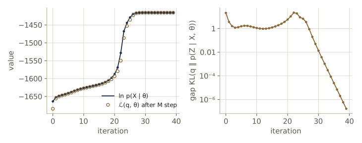
        0   -4653.33    -1684.54       20.494    -1664.04
        1   -1664.04    -1655.92        3.586    -1652.33
        2   -1652.33    -1650.00        1.573    -1648.43
        5   -1643.61    -1642.26        1.533    -1640.73
       10   -1628.56    -1627.40        1.093    -1626.30
       20   -1598.17    -1593.45        5.650    -1587.80
       39   -1415.55    -1415.55        0.000    -1415.55
The decomposition holds to rounding error at every iteration, the E step closes the gap exactly, and each M step leaves a gap \(\mathrm{KL} \ge 0\) that makes the new log likelihood higher than the new bound. The gap is largest when the parameters move most: at the first iteration (about 20), and again at iteration 22 (about 21.5, visible in the figure below), when the components separate and the log likelihood climbs fastest. Near convergence it falls by a roughly constant factor per iteration, the linear convergence typical of EM.
The picture in parameter space. As a function of \(\boldsymbol{\theta}\), the bound \(\mathcal{L}(q^{\mathrm{old}}, \boldsymbol{\theta})\) built at \(\boldsymbol{\theta}^{\mathrm{old}}\) lies below \(\ln p(\mathbf{X} \mid \boldsymbol{\theta})\) everywhere and touches it at \(\boldsymbol{\theta}^{\mathrm{old}}\). A smooth function that touches another from below must have the same gradient at the touching point, because their difference, the KL term, is nonnegative with a minimum of zero there. So
\[\nabla_{\boldsymbol{\theta}} \ln p(\mathbf{X} \mid \boldsymbol{\theta}) \Big\rvert_{\boldsymbol{\theta}^{\mathrm{old}}} = \nabla_{\boldsymbol{\theta}} \mathcal{L}(q^{\mathrm{old}}, \boldsymbol{\theta}) \Big\rvert_{\boldsymbol{\theta}^{\mathrm{old}}} = \mathbb{E}_{p(\mathbf{Z} \mid \mathbf{X}, \boldsymbol{\theta}^{\mathrm{old}})} \left[ \nabla_{\boldsymbol{\theta}} \ln p(\mathbf{X}, \mathbf{Z} \mid \boldsymbol{\theta}) \right] \Big\rvert_{\boldsymbol{\theta}^{\mathrm{old}}}.\]This is Fisher’s identity: the gradient of the marginal log likelihood is the posterior average of the complete-data gradient. We saw a special case already, when the gradient with respect to \(\boldsymbol{\mu}_k\) came out as a responsibility-weighted sum. We check it with central differences at a parameter value that is not a stationary point.
theta_0 = gmm_m_step(X, responsibilities(X, *theta_start))    # some parameter value
q_0 = responsibilities(X, *theta_0)                              # posterior there
h = 1e-5
grad_lp, grad_L = np.zeros((K, D)), np.zeros((K, D))
for k in range(K):
    for d in range(D):
        e = np.zeros((K, D)); e[k, d] = h
        up = (theta_0[0], theta_0[1] + e, theta_0[2])
        dn = (theta_0[0], theta_0[1] - e, theta_0[2])
        grad_lp[k, d] = (log_likelihood(X, *up) - log_likelihood(X, *dn)) / (2 * h)
        grad_L[k, d] = (elbo_terms(X, q_0, *up)[0] - elbo_terms(X, q_0, *dn)[0]) / (2 * h)
grad_fisher = np.stack([np.linalg.solve(theta_0[2][k], (q_0[:, [k]] * (X - theta_0[1][k])).sum(0))
                        for k in range(K)])
print("d ln p / d mu (finite differences):\n", grad_lp)
print("largest difference to d L / d mu:        ", f"{np.abs(grad_lp - grad_L).max():.1e}")
print("largest difference to the Fisher formula:", f"{np.abs(grad_lp - grad_fisher).max():.1e}")
d ln p / d mu (finite differences):
 [[11.4387 10.1619]
 [-8.9013  5.2463]
 [-3.801  -0.8899]]
largest difference to d L / d mu:         2.3e-08
largest difference to the Fisher formula: 1.1e-08
The three gradients agree to the accuracy of the finite differences. This identity is what lets deep latent-variable models be trained with gradients: we never need the gradient of the intractable \(\ln p(\mathbf{X} \mid \boldsymbol{\theta})\) directly, only gradients of the bound, whose integrand involves the joint.
Independent and identically distributed data
For i.i.d. data the joint factorizes, \(p(\mathbf{X}, \mathbf{Z} \mid \boldsymbol{\theta}) = \prod_n p(\mathbf{x}_n, \mathbf{z}_n \mid \boldsymbol{\theta})\), and so does the posterior:
\[p(\mathbf{Z} \mid \mathbf{X}, \boldsymbol{\theta}) = \frac{\prod_n p(\mathbf{x}_n, \mathbf{z}_n \mid \boldsymbol{\theta})}{\sum_{\mathbf{Z}} \prod_n p(\mathbf{x}_n, \mathbf{z}_n \mid \boldsymbol{\theta})} = \prod_{n=1}^{N} \frac{p(\mathbf{x}_n, \mathbf{z}_n \mid \boldsymbol{\theta})}{\sum_{\mathbf{z}_n} p(\mathbf{x}_n, \mathbf{z}_n \mid \boldsymbol{\theta})} = \prod_{n=1}^{N} p(\mathbf{z}_n \mid \mathbf{x}_n, \boldsymbol{\theta}),\]because the sum over all \(\mathbf{Z}\) of a product of per-point factors is the product of per-point sums. For a mixture this says that a point’s responsibilities depend only on that point and the parameters. It justified storing \(q\) as an \(N \times K\) matrix, and it means the bound is a sum of per-point bounds, \(\mathcal{L} = \sum_n \mathcal{L}_n\) with \(\mathcal{L}_n = \sum_{\mathbf{z}_n} q(\mathbf{z}_n) \ln \{ p(\mathbf{x}_n, \mathbf{z}_n \mid \boldsymbol{\theta}) / q(\mathbf{z}_n) \}\). A sum over data points can be estimated from a random minibatch of \(B\) points as \((N/B) \sum_{n \in \text{batch}} \mathcal{L}_n\), an unbiased but noisy estimate, which is how large latent-variable models are trained with stochastic gradients (module 07).
L_n = np.sum(q_0 * (log_joint(X, *theta_0) - np.log(q_0)), axis=1)   # one bound per point
print(f"sum of per-point bounds: {L_n.sum():.3f}   L(q, theta): "
      f"{elbo_terms(X, q_0, *theta_0)[0]:.3f}")
mb_rng = np.random.default_rng(5)
estimates = np.array([N / 50 * L_n[mb_rng.choice(N, size=50, replace=False)].sum()
                      for _ in range(2000)])
print(f"minibatches of 50: first estimate {estimates[0]:.1f}, mean of 2000 estimates "
      f"{estimates.mean():.1f}, standard deviation {estimates.std():.1f}")
sum of per-point bounds: -1664.043   L(q, theta): -1664.043
minibatches of 50: first estimate -1776.5, mean of 2000 estimates -1661.0, standard deviation 54.4
The per-point bounds add up to the full bound. A single minibatch of 50 points gives an estimate that can be off by a hundred nats, but the estimates average to the right value; their spread shrinks like \(1/\sqrt{B}\) (exercise 9).
Two ideas take this further in later modules. When computing the exact posterior of each \(\mathbf{z}_n\) is too expensive, we restrict \(q\) to a tractable family and maximize \(\mathcal{L}\) over that family; the gap then no longer closes, and \(\mathcal{L}\) is a genuine lower bound we optimize instead of the log likelihood. This is variational inference (Intro to ML, module 10). And instead of storing a separate \(q(\mathbf{z}_n)\) for every point, a network can compute \(q(\mathbf{z}_n \mid \mathbf{x}_n)\) from \(\mathbf{x}_n\); the variational autoencoder of module 19 does exactly this, and a diffusion model (module 20) fixes \(q\) to a known noising process and learns only \(p\).
Parameter priors
With a prior \(p(\boldsymbol{\theta})\) we maximize the log posterior \(\ln p(\boldsymbol{\theta} \mid \mathbf{X}) = \ln p(\mathbf{X} \mid \boldsymbol{\theta}) + \ln p(\boldsymbol{\theta}) - \ln p(\mathbf{X})\). The decomposition gives
\[\ln p(\boldsymbol{\theta} \mid \mathbf{X}) = \mathcal{L}(q, \boldsymbol{\theta}) + \mathrm{KL}(q \Vert p) + \ln p(\boldsymbol{\theta}) - \ln p(\mathbf{X}) \ge \mathcal{L}(q, \boldsymbol{\theta}) + \ln p(\boldsymbol{\theta}) - \ln p(\mathbf{X}),\]and \(\ln p(\mathbf{X})\) does not depend on \(\boldsymbol{\theta}\). Coordinate ascent on the right side gives MAP-EM: the prior does not involve \(q\), so the E step is unchanged, and the M step maximizes \(\mathcal{Q}(\boldsymbol{\theta}, \boldsymbol{\theta}^{\mathrm{old}}) + \ln p(\boldsymbol{\theta})\). The prior acts as a regularizer, the same role it plays for network weights in module 09.
We use it to cure the singularities. First we show EM falling into one. A sensor gets stuck and reports the same reading, \((6, -4)\), three times; those three identical points are appended to our data. We fit four components, the fourth started on the stuck reading, the others at the K-means prototypes.
X_stuck = np.vstack([X, np.tile([[6.0, -4.0]], (3, 1))])   # three identical faulty readings
theta = (np.full(4, 0.25), np.vstack([mu_km, [[6.0, -4.0]]]), np.tile(np.eye(D), (4, 1, 1)))
for it in range(20):
    gamma, ll = gmm_e_step(X_stuck, *theta)
    theta = gmm_m_step(X_stuck, gamma)
    smallest = np.linalg.eigvalsh(theta[2][3])[0]            # smallest variance of component 4
    print(f"iteration {it}: ln p = {ll:9.2f}, N_4 = {gamma[:, 3].sum():.3f}, "
          f"smallest eigenvalue of Sigma_4 = {smallest:.1e}")
    if smallest < 1e-12:
        print("Sigma_4 is singular: the next E step would divide by zero")
        break
iteration 0: ln p =  -1877.13, N_4 = 3.816, smallest eigenvalue of Sigma_4 = 2.0e-02
iteration 1: ln p =  -1485.62, N_4 = 3.486, smallest eigenvalue of Sigma_4 = 7.7e-04
iteration 2: ln p =  -1450.28, N_4 = 3.587, smallest eigenvalue of Sigma_4 = 2.7e-06
iteration 3: ln p =  -1425.55, N_4 = 3.972, smallest eigenvalue of Sigma_4 = 1.4e-09
iteration 4: ln p =  -1403.33, N_4 = 4.000, smallest eigenvalue of Sigma_4 = -5.6e-17
Sigma_4 is singular: the next E step would divide by zero
The fourth component sheds the real points it started with, until it holds the three stuck readings and one neighbor, four points in all. Any three or four points of which three coincide lie on a line, so their weighted covariance is singular, and within five iterations its smallest eigenvalue has fallen from 0.02 to zero (to rounding error). The log likelihood rises all the way, exactly as the theory promises: EM is climbing the spike.
A prior that keeps covariances away from zero fixes this. We take, for each component,
\[\ln p(\boldsymbol{\Sigma}_k) = -\frac{a}{2} \ln \lvert \boldsymbol{\Sigma}_k \rvert - \frac{b}{2} \operatorname{Tr}\left(\boldsymbol{\Sigma}_k^{-1}\right) + \text{const},\]which goes to \(-\infty\) as \(\boldsymbol{\Sigma}_k\) approaches a singular matrix (the trace term) and penalizes very large covariances (the log-determinant term). The terms of \(\mathcal{Q} + \ln p(\boldsymbol{\Sigma}_k)\) that involve \(\boldsymbol{\Sigma}_k\) are \(-\frac{N_k + a}{2} \ln \lvert \boldsymbol{\Sigma}_k \rvert - \frac{1}{2} \operatorname{Tr}\{\boldsymbol{\Sigma}_k^{-1}(N_k \mathbf{S}_k + b \mathbf{I})\}\), where \(\mathbf{S}_k\) is the ML covariance of the ordinary M step. This has the same form as a Gaussian log likelihood, so its maximum is
\[\boldsymbol{\Sigma}_k = \frac{N_k \mathbf{S}_k + b \mathbf{I}}{N_k + a}.\]It is as if every component had seen \(a\) extra points spread with covariance \((b/a) \mathbf{I}\). However few points a component owns, its covariance is at least \(b / (N_k + a)\) times the identity. We rerun the stuck-sensor example with \(a = 1\) and \(b = 0.05\), small compared with the data’s own spread, and monitor the objective \(\ln p(\mathbf{X} \mid \boldsymbol{\theta}) + \ln p(\boldsymbol{\theta})\).
def gmm_m_step_map(X, gamma, a=1.0, b=0.05):
    """M step with the prior ln p(Sigma_k) = -(a/2) ln|Sigma_k| - (b/2) Tr(Sigma_k^-1)."""
    pi, mu, S = gmm_m_step(X, gamma)                   # S_k: the ML covariances
    N_k = gamma.sum(axis=0)[:, None, None]
    return pi, mu, (N_k * S + b * np.eye(X.shape[1])) / (N_k + a)

def log_cov_prior(Sigma, a=1.0, b=0.05):
    return sum(-a / 2 * np.linalg.slogdet(S)[1] - b / 2 * np.trace(np.linalg.inv(S))
               for S in Sigma)

theta = (np.full(4, 0.25), np.vstack([mu_km, [[6.0, -4.0]]]), np.tile(np.eye(D), (4, 1, 1)))
objective = []
for it in range(200):
    gamma, ll = gmm_e_step(X_stuck, *theta)
    objective.append(ll + log_cov_prior(theta[2]))          # ln p(X | theta) + ln p(theta)
    theta = gmm_m_step_map(X_stuck, gamma)
print("ln p + ln prior never decreases:", bool(np.all(np.diff(objective) >= -1e-9)))
print(f"final objective {objective[-1]:.2f}; mixing coefficients {theta[0]}")
print("Sigma_4:\n", np.round(theta[2][3], 6) + 0.0,
      f"\nb / (N_4 + a) = {0.05 / (gamma[:, 3].sum() + 1):.4f}")
ln p + ln prior never decreases: True
final objective -1423.13; mixing coefficients [0.4784 0.1962 0.3195 0.006 ]
Sigma_4:
 [[0.0125 0.    ]
 [0.     0.0125]]
b / (N_4 + a) = 0.0125
The MAP objective climbs monotonically to a finite maximum. The fourth component still takes the three stuck readings, which is a reasonable description of these data (a separate, very tight cluster), but its covariance stops at \(b / (3 + 1) = 0.0125\) times the identity instead of collapsing, and the other three components end up essentially where the plain EM fit put them.
In practice. Library implementations of Gaussian mixtures usually add a small constant to the diagonal of every covariance after each M step. That is the MAP update above with \(a = 0\) and \(b / N_k\) held fixed, a regularizer rather than an exact prior, but it serves the same purpose. Without some such guard, EM on real data with duplicated or quantized values fails sooner or later.
Generalized EM
EM replaces one hard maximization with two easier ones, but for many models one of the two is still out of reach. The bound shows that neither step has to be complete.
The generalized EM (GEM) algorithm handles an intractable M step. Instead of maximizing \(\mathcal{L}(q, \boldsymbol{\theta})\) over \(\boldsymbol{\theta}\), it only increases it. The argument for monotonicity used only \(\mathcal{L}(q, \boldsymbol{\theta}^{\mathrm{new}}) \ge \mathcal{L}(q, \boldsymbol{\theta}^{\mathrm{old}})\), so the log likelihood still never decreases. Two standard ways to get an increase: take a few steps of a gradient-based optimizer on \(\mathcal{L}\), or maximize over one group of parameters at a time with the others fixed, which is called expectation conditional maximization (Meng and Rubin, 1993).
The gradient version is the deep learning case. When \(p(\mathbf{X} \mid \mathbf{Z}, \boldsymbol{\theta})\) is a neural network, there is no closed-form M step; we take optimizer steps on \(\mathcal{L}\). By Fisher’s identity, a single gradient step on the bound right after an exact E step is a gradient step on the log likelihood itself. So plain gradient ascent on a mixture’s log likelihood, as in module 03, is a form of GEM in which the E step is hidden inside the gradient.
To see the trade-off, we make the M step deliberately partial: the means move only a fraction \(\rho\) of the way to their M-step values, and then \(\boldsymbol{\pi}\) and \(\boldsymbol{\Sigma}\) are maximized with the new means. Because \(\mathcal{L}\) is a concave quadratic in each \(\boldsymbol{\mu}_k\) with its maximum at the weighted mean, any \(0 < \rho < 2\) increases it.
def gmm_gem(X, theta, rho, max_iter=1000, tol=1e-8):
    """Generalized EM: the means move only a fraction rho of the way to their M-step values;
    pi and Sigma are then maximized with the new means (0 < rho < 2 raises L every time)."""
    pi, mu, Sigma = theta
    ll_hist = []
    for it in range(max_iter):
        gamma, ll = gmm_e_step(X, pi, mu, Sigma)
        ll_hist.append(ll)
        if it > 0 and ll_hist[-1] - ll_hist[-2] < tol:
            break
        N_k = gamma.sum(axis=0)
        mu = mu + rho * (gamma.T @ X / N_k[:, None] - mu)    # partial step for the means
        pi = N_k / len(X)
        diff = X[None] - mu[:, None]
        Sigma = np.einsum("nk,kni,knj->kij", gamma, diff, diff) / N_k[:, None, None]
    return ll_hist

for rho in [0.25, 0.5, 1.0]:
    h = gmm_gem(X, theta_start, rho)
    print(f"rho = {rho:4.2f}: {len(h):3d} E steps to converge, final ln p = {h[-1]:.4f}, "
          f"never decreases: {bool(np.all(np.diff(h) >= -1e-9))}")
rho = 0.25: 168 E steps to converge, final ln p = -1415.5531, never decreases: True
rho = 0.50:  85 E steps to converge, final ln p = -1415.5531, never decreases: True
rho = 1.00:  45 E steps to converge, final ln p = -1415.5531, never decreases: True
All three versions climb monotonically to the same maximum; the partial steps just need more iterations, roughly in proportion to \(1/\rho\). That is the typical GEM trade: an M step that is cheaper or merely possible, at the cost of more rounds.
The E step can be partial too (Neal and Hinton, 1998). Any change of \(q\) that increases \(\mathcal{L}(q, \boldsymbol{\theta})\) keeps the ascent going, even if \(q\) does not reach the posterior. Since the bound and the log likelihood are equal exactly when \(q\) is the posterior, a global maximum of \(\mathcal{L}\) over \((q, \boldsymbol{\theta})\) gives a global maximum of \(\ln p(\mathbf{X} \mid \boldsymbol{\theta})\), and, for a joint that is continuous in \(\boldsymbol{\theta}\), local maxima correspond too. Maximizing the bound jointly is therefore a legitimate way to fit the model, whatever order the updates come in.
Sequential EM
A useful partial E step updates the responsibilities of one data point \(\mathbf{x}_m\) and then immediately does an M step. For exponential-family components the M step depends on the responsibilities only through sufficient statistics, here \(N_k = \sum_n \gamma(z_{nk})\), \(\sum_n \gamma(z_{nk}) \mathbf{x}_n\), and \(\sum_n \gamma(z_{nk}) \mathbf{x}_n \mathbf{x}_n^{\mathrm{T}}\), and changing one point’s responsibilities from \(\gamma^{\mathrm{old}}(z_{mk})\) to \(\gamma^{\mathrm{new}}(z_{mk})\) changes each statistic by one term. For the counts and means this gives
\[N_k^{\mathrm{new}} = N_k^{\mathrm{old}} + \gamma^{\mathrm{new}}(z_{mk}) - \gamma^{\mathrm{old}}(z_{mk}), \qquad \boldsymbol{\mu}_k^{\mathrm{new}} = \boldsymbol{\mu}_k^{\mathrm{old}} + \frac{\gamma^{\mathrm{new}}(z_{mk}) - \gamma^{\mathrm{old}}(z_{mk})}{N_k^{\mathrm{new}}} \left( \mathbf{x}_m - \boldsymbol{\mu}_k^{\mathrm{old}} \right),\]and the covariances follow from the second-moment statistic. Each update costs a fixed amount of work regardless of \(N\), and each E or M step raises \(\mathcal{L}\), so the guarantees carry over. This is incremental or sequential EM. We implement it with the three statistics, check that \(\mathcal{L}\) never decreases over a full pass of 500 single-point updates, and compare passes over the data with batch iterations from the same start.
def gmm_stats(X, gamma):
    """Sufficient statistics: sum_n gamma_nk, sum_n gamma_nk x_n, sum_n gamma_nk x_n x_n^T."""
    return gamma.sum(axis=0), gamma.T @ X, np.einsum("nk,ni,nj->kij", gamma, X, X)

def params_from_stats(S0, S1, S2, N):
    mu = S1 / S0[:, None]
    Sigma = S2 / S0[:, None, None] - np.einsum("ki,kj->kij", mu, mu)
    return S0 / N, mu, Sigma

def incremental_em(X, theta, passes, rng, record_bound=False):
    N = len(X)
    gamma = responsibilities(X, *theta)                   # one full E step to start
    S0, S1, S2 = gmm_stats(X, gamma)
    theta = params_from_stats(S0, S1, S2, N)
    ll_per_pass, bounds = [], []
    for _ in range(passes):
        for m in rng.permutation(N):
            g_new = responsibilities(X[m:m + 1], *theta)[0]    # E step for one point
            d = g_new - gamma[m]
            gamma[m] = g_new
            S0 = S0 + d                                        # update the statistics
            S1 = S1 + d[:, None] * X[m]
            S2 = S2 + d[:, None, None] * np.outer(X[m], X[m])
            theta = params_from_stats(S0, S1, S2, N)           # M step from the statistics
            if record_bound:
                bounds.append(elbo_terms(X, gamma, *theta)[0])
        ll_per_pass.append(log_likelihood(X, *theta))
    return theta, ll_per_pass, bounds

_, _, bounds = incremental_em(X, theta_start, 1, np.random.default_rng(6), record_bound=True)
print(f"one pass = {len(bounds)} single-point updates; "
      f"L never decreases: {bool(np.all(np.diff(bounds) >= -1e-9))}")
theta_inc, ll_inc, _ = incremental_em(X, theta_start, 20, np.random.default_rng(6))
for p in [1, 5, 10, 15, 20]:
    print(f"after {p:2d} passes: incremental ln p = {ll_inc[p - 1]:9.2f}   "
          f"batch EM ln p = {ll_em[p]:9.2f}")
target = ll_em[-1] - 0.01
print("passes to come within 0.01 of the maximum: incremental",
      int(np.argmax(np.array(ll_inc) > target)) + 1,
      " batch", int(np.argmax(np.array(ll_em) > target)))
one pass = 500 single-point updates; L never decreases: True
after  1 passes: incremental ln p =  -1650.24   batch EM ln p =  -1664.04
after  5 passes: incremental ln p =  -1629.11   batch EM ln p =  -1643.61
after 10 passes: incremental ln p =  -1606.84   batch EM ln p =  -1628.56
after 15 passes: incremental ln p =  -1419.85   batch EM ln p =  -1618.40
after 20 passes: incremental ln p =  -1415.55   batch EM ln p =  -1598.17
passes to come within 0.01 of the maximum: incremental 19  batch 32
Incremental EM gets through the plateau in fewer passes, because every point benefits immediately from the improvements made by the points before it instead of waiting for the end of a pass. In this NumPy code each pass is slower in wall-clock time than a vectorized batch iteration (500 small updates instead of one large one), so the gain is in passes over the data, which is what counts when the data are too large to hold in memory or arrive as a stream. The same logic, with the statistics replaced by exponentially weighted averages, gives the online EM algorithms used for streaming data, and it is the reason stochastic minibatch training of the bound works.
Summary
| Method | Latent variables | E step | M step | Guarantee |
|---|---|---|---|---|
| K-means | hard cluster labels | nearest prototype | cluster means | \(J\) never rises; stops in finitely many steps |
| k-means++ | (seeding) | next seed with probability \(\propto D(\mathbf{x})^2\) | expected \(J\) within \(O(\ln K)\) of optimal | |
| Vector quantization | codebook index per vector | nearest codebook vector | codebook = cluster means | \(\lceil \log_2 K \rceil\) bits per vector plus the codebook |
| Gaussian mixture EM | one-hot \(\mathbf{z}_n\) | responsibilities \(\gamma(z_{nk})\) | weighted means, covariances, \(\pi_k = N_k/N\) | \(\ln p(\mathbf{X} \mid \boldsymbol{\theta})\) never falls |
| Bernoulli mixture EM | one-hot \(\mathbf{z}_n\) | responsibilities | weighted pixel means, \(\pi_k\) | no singularities |
| ELBO | any | \(q = p(\mathbf{Z} \mid \mathbf{X}, \boldsymbol{\theta})\) closes the gap | maximize \(\mathcal{L}(q, \boldsymbol{\theta}) = \mathcal{Q} + \mathrm{H}[q]\) | the gap to \(\ln p\) is \(\mathrm{KL}(q \Vert p)\) |
| MAP-EM, GEM, incremental EM | as above | exact or one point at a time | \(\mathcal{Q} + \ln p(\boldsymbol{\theta})\), or any increase of \(\mathcal{L}\) | objective never falls |
Ideas to carry forward:
- A latent variable turns a marginal likelihood with a sum inside the logarithm into a complete-data likelihood that is easy to maximize. EM alternates between inferring the latent variables (the posterior) and refitting the parameters as if the inferred values were data.
- \(\ln p(\mathbf{X} \mid \boldsymbol{\theta}) = \mathcal{L}(q, \boldsymbol{\theta}) + \mathrm{KL}(q \Vert p)\) holds for every \(q\). Anything that raises \(\mathcal{L}\) (a full or partial E step, a full or partial M step, a gradient step) is progress. Variational autoencoders and diffusion models optimize this same bound with \(q\) and \(p\) given by networks.
- After an exact E step the bound touches the log likelihood with the same gradient (Fisher’s identity), which is why gradient-based training of latent-variable models works.
- Maximum likelihood for mixtures has degenerate spikes and \(K!\) symmetric copies of every solution. Seeding, several restarts, and a prior or variance floor are part of the method, not afterthoughts.
Exercises
- Prove that K-means cannot revisit an assignment once it has left it, and conclude that it stops after at most \(K^N\) iterations. Then construct four points on a line and a starting pair of prototypes for \(K = 2\) for which K-means stops at an assignment whose distortion is more than twice the optimum.
- Show that the sequential update with step \(1/N_k\) keeps each prototype equal to the mean of the points assigned to it so far. Then replace \(1/N_k\) by a constant \(\eta\) and run sequential K-means on the MNIST patches with \(K = 32\) for one pass, for \(\eta = 0.01, 0.05, 0.2\). Compare the final distortion with batch K-means and explain the effect of \(\eta\).
- Suppose all components of a Gaussian mixture share one covariance matrix \(\boldsymbol{\Sigma}\). Derive the M-step update for \(\boldsymbol{\Sigma}\) from \(\mathcal{Q}\), modify
gmm_m_step, and fit the three-cluster data. How does the log likelihood compare with the full model, and which cluster suffers most? - The code computes \(\ln \mathcal{N}\) with a Cholesky factor and combines components with log-sum-exp. Replace both with the direct formulas (
np.linalg.inv,np.exp, thennp.logof the sum) and find a point, or a component variance, at which the direct version returns-infornanwhile the log-space version is fine. - For the mixture with covariances \(\epsilon \mathbf{I}\), show that \(\epsilon \, \mathcal{Q}(\boldsymbol{\theta}, \boldsymbol{\theta}^{\mathrm{old}}) \to -\frac{1}{2} J\) as \(\epsilon \to 0\), where the responsibilities are computed with the same \(\epsilon\). Which term of the Gaussian’s normalizing constant makes the convergence slow? Check your answer numerically with
em_shared_variance. - For any mixture \(p(\mathbf{x}) = \sum_k \pi_k p_k(\mathbf{x})\) whose components have means \(\boldsymbol{\mu}_k\) and covariances \(\boldsymbol{\Sigma}_k\), prove the formula for \(\operatorname{cov}[\mathbf{x}]\) given for Bernoulli mixtures. Then compute the covariance of two neighboring pixels in the center of the image under the fitted ten-component Bernoulli mixture and under the single Bernoulli, and compare both with the sample covariance of the 2000 binary digits.
- Put a prior \(\mathrm{Beta}(\mu_{ki} \mid \alpha, \alpha)\) on every pixel probability of the Bernoulli mixture. Derive the MAP M step (it adds pseudo-counts), implement it, and show that with \(\alpha = 2\) the clipping in
bernoulli_emis no longer needed. How do the learned means change? - Prove Fisher’s identity \(\nabla_{\boldsymbol{\theta}} \ln p(\mathbf{X} \mid \boldsymbol{\theta}) = \mathbb{E}_{p(\mathbf{Z} \mid \mathbf{X}, \boldsymbol{\theta})}[\nabla_{\boldsymbol{\theta}} \ln p(\mathbf{X}, \mathbf{Z} \mid \boldsymbol{\theta})]\) directly, by differentiating \(\ln \sum_{\mathbf{Z}} p(\mathbf{X}, \mathbf{Z} \mid \boldsymbol{\theta})\). Then use it to fit the means of the three-cluster mixture by gradient ascent (covariances and weights fixed at the EM solution, means started at
mu_start), and count the iterations needed to reach the EM means to three decimals with the best step size you can find. - Measure the standard deviation of the minibatch estimate \((N/B) \sum_{n \in \text{batch}} \mathcal{L}_n\) for \(B = 10, 50, 250\) and compare with the \(1/\sqrt{B}\) rule, including the correction for sampling without replacement. What happens at \(B = N\)?
- Derive the incremental update for the covariance of component \(k\) from the second-moment statistic, as a formula in \(\boldsymbol{\Sigma}_k^{\mathrm{old}}\), \(\boldsymbol{\mu}_k^{\mathrm{old}}\), \(\boldsymbol{\mu}_k^{\mathrm{new}}\), and the change in responsibility. Then check
incremental_emagainst batch statistics: after a full pass, recompute the three statistics from the storedgammaand verify they match the running ones. - Split the three-cluster data into 350 training and 150 held-out points. Fit mixtures with \(K = 1, \dots, 6\) (five k-means++ starts each, the MAP M step with \(a = 1\), \(b = 0.05\)), and plot the training and held-out log likelihood per point against \(K\). Which \(K\) would you choose, and why can the training curve not tell you?
- In your own words: explain why EM never decreases the log likelihood even though it never computes a gradient, what the KL term in the decomposition measures, and why the same bound can still be used when the posterior over the latent variables cannot be computed.
Going further
- Bishop & Bishop, Deep Learning: Foundations and Concepts, chapter 15 — the source for this module. Exercises 15.1–15.2 treat K-means convergence and its sequential form, 15.3–15.4 the latent-variable form and label symmetry, 15.5–15.10 the general and Gaussian-mixture EM steps, 15.12 the K-means limit, 15.13–15.20 Bernoulli and multinomial mixtures, 15.21–15.22 the evidence lower bound and its gradient, and 15.23–15.24 incremental EM.
- Intro to ML, module 09 — the same chapter of PRML at greater length: K-medoids, online K-means, sampling from mixtures, EM for Bayesian linear regression, and the bound drawn as a curve in parameter space. Intro to ML, module 10 continues from the bound to variational inference.
- A. P. Dempster, N. M. Laird, and D. B. Rubin, “Maximum likelihood from incomplete data via the EM algorithm”, Journal of the Royal Statistical Society, Series B, 1977 — the paper that named EM and stated it in general.
- R. M. Neal and G. E. Hinton, “A view of the EM algorithm that justifies incremental, sparse, and other variants,” in M. I. Jordan (ed.), Learning in Graphical Models, 1998 — EM as coordinate ascent on the lower bound, the view of the last part of this module.
- D. Arthur and S. Vassilvitskii, “k-means++: the advantages of careful seeding,” Proceedings of the ACM-SIAM Symposium on Discrete Algorithms, 2007 — the seeding rule and its \(O(\ln K)\) guarantee.
- A. van den Oord, O. Vinyals, and K. Kavukcuoglu, “Neural discrete representation learning,” NeurIPS 2017, arXiv:1711.00937 — the VQ-VAE, a learned codebook of discrete latents inside an autoencoder.
- In this course, the bound returns with continuous latent variables in module 16, with a network-computed \(q\) in module 19, and with a fixed noising \(q\) in module 20.
These notes follow the chapters of C. M. Bishop and H. Bishop, Deep Learning: Foundations and Concepts (Springer, 2024), the course text, which the authors make free to read online. The explanations, code, figures, and exercises here are written for this course; the book remains the reference, with the full derivations and many more exercises.