CSE 676 · Module 16 · Week 12
Continuous Latent Variables
Principal component analysis, probabilistic PCA and factor analysis, ICA and Kalman filters, EM for linear-Gaussian models, and nonlinear latent-variable models.
Companion reading: Bishop & Bishop, Deep Learning: Foundations and Concepts, chapter 16, “Continuous Latent Variables”
By the end of this module you can
- Derive principal component analysis as the projection of maximum variance and as the projection of minimum reconstruction error, compute it by eigendecomposition and by the SVD, and use it to compress and whiten data.
- Apply the Gram-matrix trick when there are fewer data points than dimensions, and check that it gives the same eigenvalues and eigenvectors.
- Write down probabilistic PCA as a generative model, derive its marginal covariance and posterior, and compute its closed-form maximum likelihood solution, including its rotational non-identifiability.
- Explain how factor analysis, independent component analysis, and the Kalman filter change one assumption of probabilistic PCA each, and run a small blind-source-separation and tracking example.
- Derive the evidence lower bound for continuous latent variables and implement EM for probabilistic PCA, for zero-noise PCA, and for factor analysis.
- Explain why the likelihood of a nonlinear latent-variable model \(p(\mathbf{x}) = \int p(\mathbf{x} \mid \mathbf{z}, \mathbf{w}) \, p(\mathbf{z}) \, d\mathbf{z}\) is intractable, and measure how badly naive Monte Carlo estimates it.
- Choose output distributions for discrete data and explain why dequantization is needed for flexible density models of quantized values.
- Compare generative adversarial networks, normalizing flows, variational autoencoders, and diffusion models by what each gives up to make training possible.
Contents
- Principal component analysis
- Probabilistic latent variables
- The evidence lower bound
- Nonlinear latent-variable models
- Summary
- Exercises
- Going further
In module 15 each data point came with a hidden label, the mixture component that produced it, and the evidence lower bound turned maximum likelihood with such hidden labels into the EM algorithm. This module keeps the idea of an unobserved cause but lets it be a continuous vector \(\mathbf{z}\). The motivation is geometric. A \(28 \times 28\) image of a handwritten digit is a point in a 784-dimensional space, yet the images a person could plausibly write fill only a thin region of that space: a small number of smooth changes (slant, thickness, the size of a loop, a shift of position) move one digit into another. Data of this kind lie close to a manifold, a smooth surface whose dimension is much lower than the number of measured variables, and the coordinates on that surface are natural latent variables.
The first half of the module is the linear, Gaussian part of the story, much of which you may have met in Intro to ML, module 12: principal component analysis (PCA), its probabilistic version, factor analysis, independent component analysis, the Kalman filter, and EM for these models. We keep that part compact, run everything on MNIST or on small synthetic data, and point to the ML notes for longer derivations. The second half leaves the linear world. If the map from \(\mathbf{z}\) to \(\mathbf{x}\) is a deep network, sampling stays easy but the likelihood stops being computable, and the four ways around that problem are the subjects of the last four modules of the course.
Everything here is NumPy. SciPy supplies a few linear-algebra helpers, and torchvision only loads MNIST.
Principal component analysis
Principal component analysis (PCA) finds a linear subspace of dimension \(M < D\), the principal subspace, onto which the data can be projected with as little loss as possible. “As little loss as possible” can be made precise in two ways, and both lead to the same answer: the eigenvectors of the data covariance matrix with the largest eigenvalues.
Maximum-variance formulation
Take data \(\mathbf{x}_1, \dots, \mathbf{x}_N \in \mathbb{R}^D\) with mean \(\bar{\mathbf{x}} = \frac{1}{N}\sum_n \mathbf{x}_n\) and covariance
\[\mathbf{S} = \frac{1}{N} \sum_{n=1}^{N} (\mathbf{x}_n - \bar{\mathbf{x}})(\mathbf{x}_n - \bar{\mathbf{x}})^{\mathrm{T}} .\]Start with one direction, a unit vector \(\mathbf{u}_1\). Projecting each point onto it gives the scalars \(\mathbf{u}_1^{\mathrm{T}}\mathbf{x}_n\), whose mean is \(\mathbf{u}_1^{\mathrm{T}}\bar{\mathbf{x}}\) and whose variance is
\[\frac{1}{N}\sum_{n=1}^{N} \left(\mathbf{u}_1^{\mathrm{T}}\mathbf{x}_n - \mathbf{u}_1^{\mathrm{T}}\bar{\mathbf{x}}\right)^2 = \mathbf{u}_1^{\mathrm{T}} \mathbf{S} \mathbf{u}_1 .\]We want the direction that keeps the most spread. Without a constraint the variance grows without bound as \(\lVert \mathbf{u}_1 \rVert\) grows, so we fix \(\mathbf{u}_1^{\mathrm{T}}\mathbf{u}_1 = 1\) with a Lagrange multiplier \(\lambda_1\) and maximize \(\mathbf{u}_1^{\mathrm{T}}\mathbf{S}\mathbf{u}_1 + \lambda_1(1 - \mathbf{u}_1^{\mathrm{T}}\mathbf{u}_1)\). The gradient with respect to \(\mathbf{u}_1\) is \(2\mathbf{S}\mathbf{u}_1 - 2\lambda_1\mathbf{u}_1\), and setting it to zero gives
\[\mathbf{S}\mathbf{u}_1 = \lambda_1 \mathbf{u}_1 .\]So \(\mathbf{u}_1\) must be an eigenvector of \(\mathbf{S}\). Multiplying on the left by \(\mathbf{u}_1^{\mathrm{T}}\) shows that the projected variance equals the eigenvalue, \(\mathbf{u}_1^{\mathrm{T}}\mathbf{S}\mathbf{u}_1 = \lambda_1\), so the best choice is the eigenvector with the largest eigenvalue: the first principal component. Asking next for the direction of largest variance orthogonal to \(\mathbf{u}_1\) gives the eigenvector with the second largest eigenvalue, and by induction (exercise 1) the best \(M\)-dimensional projection is spanned by the \(M\) leading eigenvectors \(\mathbf{u}_1, \dots, \mathbf{u}_M\) of \(\mathbf{S}\). Because \(\mathbf{S}\) is symmetric, they can be chosen orthonormal.
Let us check this on a cloud of 200 correlated points in the plane, by comparing the eigenvector with a brute-force search over directions.
import numpy as np
from scipy import linalg
from scipy.special import logsumexp
from torchvision import datasets

np.set_printoptions(precision=4, suppress=True)
rng = np.random.default_rng(16)

def make_blob(N, gen):
    """N correlated points in 2-D: a standard Gaussian stretched along an oblique direction."""
    L = np.array([[2.0, 0.0], [1.2, 0.6]])
    return gen.standard_normal((N, 2)) @ L.T + np.array([1.0, -0.5])

def pca_eig(X):
    """Mean, eigenvalues (largest first), and eigenvectors (as columns) of the covariance of X."""
    xbar = X.mean(axis=0)
    Xc = X - xbar
    S = Xc.T @ Xc / len(X)                        # data covariance matrix S
    lam, U = np.linalg.eigh(S)                    # eigh returns ascending eigenvalues
    order = np.argsort(lam)[::-1]
    return xbar, lam[order], U[:, order]

X2 = make_blob(200, rng)
xbar2, lam2, U2 = pca_eig(X2)
print("eigenvalues:", lam2)

theta = np.linspace(0, np.pi, 3601)               # candidate directions, 0.05 degrees apart
dirs = np.column_stack([np.cos(theta), np.sin(theta)])
Xc2 = X2 - xbar2
proj_var = np.mean((Xc2 @ dirs.T) ** 2, axis=0)   # u^T S u for every candidate u
best = np.argmax(proj_var)
print(f"search: best angle {np.degrees(theta[best]):.2f} deg, variance {proj_var[best]:.4f}")
angle_u1 = np.degrees(np.arctan2(U2[1, 0], U2[0, 0])) % 180
print(f"PCA:    u_1 angle  {angle_u1:.2f} deg, lambda_1 {lam2[0]:.4f}")
eigenvalues: [5.921  0.2296]
search: best angle 32.55 deg, variance 5.9210
PCA:    u_1 angle  32.57 deg, lambda_1 5.9210
The search, limited to a grid of angles 0.05° apart, lands within that resolution of \(\mathbf{u}_1\), and the best variance it finds matches \(\lambda_1\).
Minimum-error formulation
The second definition asks for the subspace that approximates the data points best. Complete the directions to an orthonormal basis \(\mathbf{u}_1, \dots, \mathbf{u}_D\) of \(\mathbb{R}^D\). Any point can be written exactly as \(\mathbf{x}_n = \sum_{i=1}^{D} (\mathbf{x}_n^{\mathrm{T}}\mathbf{u}_i)\,\mathbf{u}_i\). To compress, we keep \(M\) coefficients per point and replace the rest by constants shared by all points:
\[\tilde{\mathbf{x}}_n = \sum_{i=1}^{M} z_{ni}\,\mathbf{u}_i + \sum_{i=M+1}^{D} b_i\,\mathbf{u}_i , \qquad J = \frac{1}{N}\sum_{n=1}^{N} \lVert \mathbf{x}_n - \tilde{\mathbf{x}}_n \rVert^2 .\]We minimize the average squared error \(J\) over the coefficients, the constants, and the basis. Because the basis is orthonormal, \(J\) splits into one squared term per direction. Setting derivatives to zero gives \(z_{nj} = \mathbf{x}_n^{\mathrm{T}}\mathbf{u}_j\) for the kept directions (project each point) and \(b_j = \bar{\mathbf{x}}^{\mathrm{T}}\mathbf{u}_j\) for the discarded ones (use the mean’s coordinate). The residual is then
\[\mathbf{x}_n - \tilde{\mathbf{x}}_n = \sum_{i=M+1}^{D} \left\{ (\mathbf{x}_n - \bar{\mathbf{x}})^{\mathrm{T}}\mathbf{u}_i \right\} \mathbf{u}_i ,\]which lies entirely in the discarded directions, so the best approximation is an orthogonal projection onto a subspace through the mean. Substituting back,
\[J = \frac{1}{N}\sum_{n=1}^{N}\sum_{i=M+1}^{D} \left\{ (\mathbf{x}_n - \bar{\mathbf{x}})^{\mathrm{T}}\mathbf{u}_i \right\}^2 = \sum_{i=M+1}^{D} \mathbf{u}_i^{\mathrm{T}}\mathbf{S}\mathbf{u}_i .\]Minimizing this subject to orthonormality is the maximum-variance problem turned around: each discarded \(\mathbf{u}_i\) must again be an eigenvector (the Lagrange argument above, with a minimum instead of a maximum), and the error is the sum of the discarded eigenvalues.
Result. Keeping the \(M\) leading eigenvectors of \(\mathbf{S}\) gives both the largest projected variance and the smallest reconstruction error, and the error is what is thrown away:
\[J = \sum_{i=M+1}^{D} \lambda_i .\]
The two definitions agree because they add up to a constant. The total variance \(\frac{1}{N}\sum_n \lVert \mathbf{x}_n - \bar{\mathbf{x}} \rVert^2 = \operatorname{Tr}(\mathbf{S}) = \sum_i \lambda_i\) does not depend on the subspace, and it is split exactly into the variance kept and the error made. On the 2-D cloud:
proj_err = np.mean(np.sum(Xc2 ** 2, axis=1)) - proj_var   # mean squared distance to each line
worst = np.argmin(proj_err)
print(f"smallest error {proj_err[worst]:.4f} at {np.degrees(theta[worst]):.2f} deg;"
      f" lambda_2 = {lam2[1]:.4f}")
print(f"variance + error = {proj_var[worst] + proj_err[worst]:.4f} = Tr(S) = {lam2.sum():.4f}")
smallest error 0.2296 at 32.55 deg; lambda_2 = 0.2296
variance + error = 6.1506 = Tr(S) = 6.1506
A related method, canonical correlation analysis, works with two sets of variables measured on the same items and looks for a pair of subspaces, one per set, whose coordinates are maximally correlated; it also reduces to an eigenvalue problem (a generalized one). Bishop & Bishop §16.1.2 gives references.
In practice PCA is usually computed from the singular value decomposition (SVD) of the centered data matrix rather than from \(\mathbf{S}\). Write the centered data as the \(N \times D\) matrix \(\tilde{\mathbf{X}}\) with rows \((\mathbf{x}_n - \bar{\mathbf{x}})^{\mathrm{T}}\), and its thin SVD as \(\tilde{\mathbf{X}} = \mathbf{P}\boldsymbol{\Sigma}\mathbf{Q}^{\mathrm{T}}\). Then \(\mathbf{S} = \frac{1}{N}\tilde{\mathbf{X}}^{\mathrm{T}}\tilde{\mathbf{X}} = \mathbf{Q}\,\frac{\boldsymbol{\Sigma}^2}{N}\,\mathbf{Q}^{\mathrm{T}}\), so the right singular vectors are the principal directions and \(\lambda_i = s_i^2/N\), where \(s_i\) are the singular values. The SVD never forms \(\mathbf{S}\), and so avoids squaring the condition number of the data matrix, which roughly halves the number of significant digits lost to rounding. Let us load 6,000 MNIST digits (\(D = 784\)) and check that the two routes agree.
train = datasets.MNIST(root="data", train=True, download=True)
X = train.data[:6000].float().div(255.).reshape(6000, -1).numpy().astype(np.float64)
labels = train.targets[:6000].numpy()
N, D = X.shape

def pca_svd(X):
    """PCA from the thin SVD of the centered data: directions = right singular vectors."""
    xbar = X.mean(axis=0)
    _, s, Qt = np.linalg.svd(X - xbar, full_matrices=False)
    return xbar, s ** 2 / len(X), Qt.T

xbar, lam, U = pca_eig(X)
_, lam_svd, U_svd = pca_svd(X)
k = 50
print("data:", X.shape, "  leading eigenvalues:", lam[:5])
print(f"max eigenvalue difference, first {k}: {np.max(np.abs(lam[:k] - lam_svd[:k])):.1e}")
cosines = np.abs(np.sum(U[:, :k] * U_svd[:, :k], axis=0))   # eigenvectors agree up to sign
print(f"smallest cosine between matching directions: {cosines.min():.12f}")
print("nonzero eigenvalues:", np.sum(lam > 1e-10 * lam[0]), "of", D)
data: (6000, 784)   leading eigenvalues: [5.3047 3.8764 3.2865 2.9121 2.4859]
max eigenvalue difference, first 50: 6.2e-15
smallest cosine between matching directions: 1.000000000000
nonzero eigenvalues: 655 of 784
The eigenvectors agree up to sign, which is all that can be asked: \(-\mathbf{u}_i\) is as good an eigenvector as \(\mathbf{u}_i\). Note also that 129 eigenvalues are zero to rounding error. Most of them come from the 120 pixels near the border that are blank in every one of these 6,000 images, so the data have no variance at all along those coordinates; a handful of other directions carry variance too small to register.
Data compression
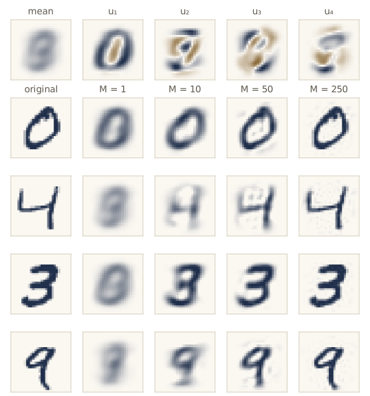
Each principal direction \(\mathbf{u}_i\) is a vector in pixel space, so it can be displayed as an image, and the reconstruction of a digit from \(M\) coefficients is
\[\tilde{\mathbf{x}}_n = \bar{\mathbf{x}} + \sum_{i=1}^{M} \left\{ (\mathbf{x}_n - \bar{\mathbf{x}})^{\mathrm{T}}\mathbf{u}_i \right\} \mathbf{u}_i .\]This is lossy compression: each image is stored as \(M\) numbers instead of \(D\), plus the mean and \(M\) directions shared by the whole data set. In network terms it is a two-layer linear map, an encoder \(\mathbf{z}_n = \mathbf{U}_M^{\mathrm{T}}(\mathbf{x}_n - \bar{\mathbf{x}})\) followed by a decoder \(\bar{\mathbf{x}} + \mathbf{U}_M \mathbf{z}_n\), where \(\mathbf{U}_M\) holds the first \(M\) eigenvectors as columns. We will meet the nonlinear version, the autoencoder, in module 19.
def pca_encode(X, xbar, U, M):
    """Principal coordinates z_ni = (x_n - xbar)^T u_i for i = 1..M."""
    return (X - xbar) @ U[:, :M]

def pca_decode(Z, xbar, U):
    """Reconstruction xbar + sum_i z_ni u_i."""
    return xbar + Z @ U[:, :Z.shape[1]].T

for M in [1, 10, 50, 250]:
    X_rec = pca_decode(pca_encode(X, xbar, U, M), xbar, U)
    J = np.mean(np.sum((X - X_rec) ** 2, axis=1))
    kept = 1 - lam[M:].sum() / lam.sum()
    print(f"M = {M:3d}:  J = {J:7.4f}   sum of discarded eigenvalues = {lam[M:].sum():7.4f}"
          f"   variance kept = {kept:.3f}")
cum = np.cumsum(lam) / lam.sum()
for f in [0.8, 0.9, 0.95, 0.99]:
    print(f"components needed for {f:.0%} of the variance: {np.searchsorted(cum, f) + 1}")
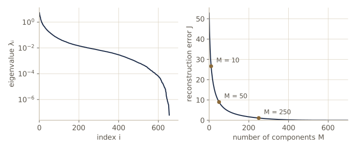
M =   1:  J = 47.5369   sum of discarded eigenvalues = 47.5369   variance kept = 0.100
M =  10:  J = 26.6254   sum of discarded eigenvalues = 26.6254   variance kept = 0.496
M =  50:  J =  8.9751   sum of discarded eigenvalues =  8.9751   variance kept = 0.830
M = 250:  J =  1.0793   sum of discarded eigenvalues =  1.0793   variance kept = 0.980
components needed for 80% of the variance: 42
components needed for 90% of the variance: 84
components needed for 95% of the variance: 149
components needed for 99% of the variance: 323
The measured reconstruction error equals the sum of the discarded eigenvalues, as the result above says it must. The spectrum falls quickly at first and then has a long tail: 10 components keep about half of the variance, but reaching 99% takes a few hundred.
Data whitening
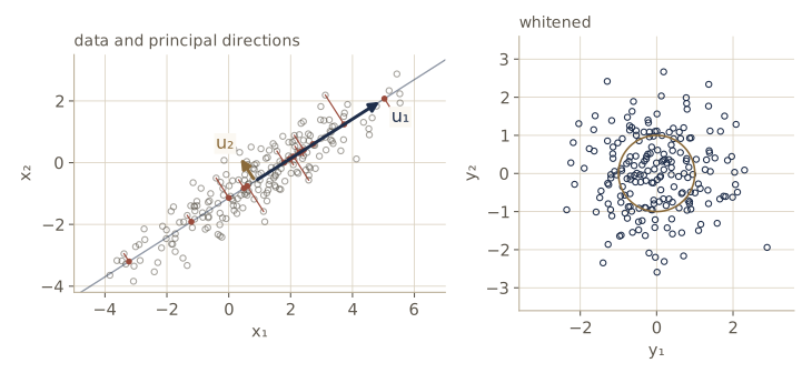
PCA is also used to preprocess data rather than to reduce their dimension. The mildest version is standardizing: shift and scale each variable separately to zero mean and unit variance. The covariance of standardized data is the correlation matrix of the original variables, with entries \(\rho_{ij}\) between \(-1\) and \(1\); standardizing removes differences of scale but not correlations.
Whitening (or sphering) goes further. Collect the eigenvectors in the orthogonal matrix \(\mathbf{U}\) and the eigenvalues in the diagonal matrix \(\mathbf{L}\), so that \(\mathbf{S}\mathbf{U} = \mathbf{U}\mathbf{L}\), and map each point to
\[\mathbf{y}_n = \mathbf{L}^{-1/2}\mathbf{U}^{\mathrm{T}}(\mathbf{x}_n - \bar{\mathbf{x}}) .\]The new points have zero mean, and their covariance is \(\frac{1}{N}\sum_n \mathbf{y}_n\mathbf{y}_n^{\mathrm{T}} = \mathbf{L}^{-1/2}\mathbf{U}^{\mathrm{T}}\mathbf{S}\mathbf{U}\mathbf{L}^{-1/2} = \mathbf{L}^{-1/2}\mathbf{L}\mathbf{L}^{-1/2} = \mathbf{I}\): rotate onto the principal axes, then rescale each axis to unit variance.
def whiten(X, xbar, lam, U):
    """y_n = L^{-1/2} U^T (x_n - xbar), one row per point."""
    return (X - xbar) @ U / np.sqrt(lam)

X_std = (X2 - xbar2) / X2.std(axis=0)
Y2 = whiten(X2, xbar2, lam2, U2)
print("covariance after standardizing:\n", X_std.T @ X_std / len(X_std))
print("covariance after whitening:\n", Y2.T @ Y2 / len(Y2))
covariance after standardizing:
 [[1.     0.9114]
 [0.9114 1.    ]]
covariance after whitening:
 [[1. 0.]
 [0. 1.]]
The standardized cloud still has a correlation of about 0.9 between its coordinates; the whitened one has none. Whitening is the first step of independent component analysis later in this module. In deep networks, the normalization layers of module 07 standardize each variable separately rather than whitening, because a full whitening transform would need the eigendecomposition of a large covariance matrix at every step.
Watch out. Whitening divides by \(\sqrt{\lambda_i}\). On MNIST more than a hundred eigenvalues are exactly zero and many more are tiny, so whitening the raw pixels either fails or blows noise up to unit variance. In practice one keeps only the leading \(M\) components, or adds a small constant to every eigenvalue before dividing.
High-dimensional data
Sometimes there are fewer data points than dimensions, \(N < D\): a few hundred high-resolution images, say. Then \(N\) points span an affine subspace of dimension at most \(N - 1\), so at least \(D - N + 1\) eigenvalues of \(\mathbf{S}\) are zero, and the \(O(D^3)\) cost of eigendecomposing a \(D \times D\) matrix is spent mostly on nothing.
The fix works with the \(N \times N\) matrix instead. The eigenvector equation is \(\frac{1}{N}\tilde{\mathbf{X}}^{\mathrm{T}}\tilde{\mathbf{X}}\mathbf{u}_i = \lambda_i\mathbf{u}_i\). Multiply both sides on the left by \(\tilde{\mathbf{X}}\) and write \(\mathbf{v}_i = \tilde{\mathbf{X}}\mathbf{u}_i\):
\[\frac{1}{N}\tilde{\mathbf{X}}\tilde{\mathbf{X}}^{\mathrm{T}}\mathbf{v}_i = \lambda_i \mathbf{v}_i .\]So the nonzero eigenvalues of the Gram matrix \(\frac{1}{N}\tilde{\mathbf{X}}\tilde{\mathbf{X}}^{\mathrm{T}}\), whose entries are inner products between data points, are the same as those of \(\mathbf{S}\), and they cost \(O(N^3)\) to find. To get back to data space, multiply the Gram equation on the left by \(\tilde{\mathbf{X}}^{\mathrm{T}}\): it says that \(\tilde{\mathbf{X}}^{\mathrm{T}}\mathbf{v}_i\) is an eigenvector of \(\mathbf{S}\) with eigenvalue \(\lambda_i\). If \(\mathbf{v}_i\) has unit length, then \(\lVert \tilde{\mathbf{X}}^{\mathrm{T}}\mathbf{v}_i \rVert^2 = \mathbf{v}_i^{\mathrm{T}}\tilde{\mathbf{X}}\tilde{\mathbf{X}}^{\mathrm{T}}\mathbf{v}_i = N\lambda_i\), so the normalized eigenvector is
\[\mathbf{u}_i = \frac{1}{(N\lambda_i)^{1/2}}\,\tilde{\mathbf{X}}^{\mathrm{T}}\mathbf{v}_i .\]We check it on 300 digits, where \(N = 300 < D = 784\).
def pca_gram(X, M):
    """Leading M eigenpairs of S from the N x N Gram matrix (useful when N < D)."""
    xbar = X.mean(axis=0)
    Xc = X - xbar
    K = Xc @ Xc.T / len(X)                               # (1/N) X X^T
    mu, V = np.linalg.eigh(K)
    order = np.argsort(mu)[::-1][:M]
    mu, V = mu[order], V[:, order]
    return xbar, mu, Xc.T @ V / np.sqrt(len(X) * mu)     # u_i = X^T v_i / sqrt(N lambda_i)

X_small = X[:300]
_, lam_g, U_g = pca_gram(X_small, 50)
_, lam_d, U_d = pca_eig(X_small)
print(f"max eigenvalue difference: {np.max(np.abs(lam_g - lam_d[:50])):.1e}")
cos_g = np.abs(np.sum(U_g * U_d[:, :50], axis=0))
print(f"smallest cosine between directions: {cos_g.min():.12f}")
print(f"direction lengths between {np.linalg.norm(U_g, axis=0).min():.6f}"
      f" and {np.linalg.norm(U_g, axis=0).max():.6f}")
print("nonzero eigenvalues of S:", np.sum(lam_d > 1e-10 * lam_d[0]),
      "(N - 1 =", len(X_small) - 1, ")")
max eigenvalue difference: 2.7e-15
smallest cosine between directions: 1.000000000000
direction lengths between 1.000000 and 1.000000
nonzero eigenvalues of S: 299 (N - 1 = 299 )
Only \(N - 1 = 299\) eigenvalues are nonzero: centering removes one more dimension. The same trick, applied with a kernel in place of the inner product, gives kernel PCA (Intro to ML, module 12).
Probabilistic latent variables
So far PCA is a projection recipe. It has no density: it cannot say how probable a new image is, it cannot generate new data, and it has no likelihood with which to compare it to other models. Recasting PCA as a latent-variable model, a joint distribution over an observed \(\mathbf{x}\) and a hidden \(\mathbf{z}\), gives it all of these, and opens the door to EM, to missing data, to mixtures of PCA models, and to a Bayesian choice of \(M\) (Intro to ML, module 12 covers the last). More important for this course, it is the linear template for every deep generative model in modules 17–20.
The generative model
Probabilistic PCA (PPCA) says each data point is made in two steps. First draw an \(M\)-dimensional latent vector from a standard Gaussian; then map it linearly into data space and add isotropic Gaussian noise:
\[p(\mathbf{z}) = \mathcal{N}(\mathbf{z} \mid \mathbf{0}, \mathbf{I}), \qquad p(\mathbf{x} \mid \mathbf{z}) = \mathcal{N}(\mathbf{x} \mid \mathbf{W}\mathbf{z} + \boldsymbol{\mu}, \sigma^2\mathbf{I}),\]or equivalently \(\mathbf{x} = \mathbf{W}\mathbf{z} + \boldsymbol{\mu} + \boldsymbol{\epsilon}\) with \(\boldsymbol{\epsilon} \sim \mathcal{N}(\mathbf{0}, \sigma^2\mathbf{I})\) independent of \(\mathbf{z}\). The parameters are the \(D \times M\) matrix \(\mathbf{W}\), the offset \(\boldsymbol{\mu}\), and the noise variance \(\sigma^2\). The columns of \(\mathbf{W}\) span a plane in data space, the prior spreads points over that plane, and the noise blurs them off it. Because the noise covariance is diagonal, the components of \(\mathbf{x}\) are independent once \(\mathbf{z}\) is known: all correlations between observed variables are explained by the latent variables.
Choosing a standard Gaussian for \(\mathbf{z}\) costs no generality. A latent \(\mathcal{N}(\mathbf{m}, \boldsymbol{\Sigma})\) can be written as \(\mathbf{m} + \boldsymbol{\Sigma}^{1/2}\mathbf{z}'\) with standard \(\mathbf{z}'\), and the extra shift and scaling are absorbed into \(\boldsymbol{\mu}\) and \(\mathbf{W}\).
The model is defined from latent space to data space, the opposite direction from the projection of the last section, and that makes sampling immediate: this is ancestral sampling, drawing each variable given its parents in the graph.
def ppca_sample(W, mu, sigma2, N, gen):
    """Ancestral sampling: z ~ N(0, I), then x = W z + mu + eps with eps ~ N(0, sigma2 I)."""
    Z = gen.standard_normal((N, W.shape[1]))
    X = Z @ W.T + mu + np.sqrt(sigma2) * gen.standard_normal((N, W.shape[0]))
    return X, Z

W_toy = np.array([[2.0, 0.0], [1.0, 1.0], [0.0, 1.5], [-1.0, 0.5], [0.5, -0.5]])   # D = 5, M = 2
mu_toy, s2_toy = np.array([1.0, 0.0, -1.0, 2.0, 0.0]), 0.2
X_toy, Z_toy = ppca_sample(W_toy, mu_toy, s2_toy, 200_000, rng)
print("first sample x:", X_toy[0], "  from z:", Z_toy[0])
first sample x: [ 0.7623 -1.0488 -2.5602 2.6343 -0.6558] from z: [-0.2277 -0.3395]
Likelihood function
To fit the model by maximum likelihood we need the marginal \(p(\mathbf{x}) = \int p(\mathbf{x} \mid \mathbf{z})\,p(\mathbf{z})\,d\mathbf{z}\). This is a linear-Gaussian model, so the marginal is Gaussian (module 03 derived the general identity), and we only need its mean and covariance. From \(\mathbf{x} = \mathbf{W}\mathbf{z} + \boldsymbol{\mu} + \boldsymbol{\epsilon}\) with \(\mathbf{z}\) and \(\boldsymbol{\epsilon}\) independent and zero-mean,
\[\mathbb{E}[\mathbf{x}] = \boldsymbol{\mu}, \qquad \operatorname{cov}[\mathbf{x}] = \mathbb{E}\left[(\mathbf{W}\mathbf{z} + \boldsymbol{\epsilon})(\mathbf{W}\mathbf{z} + \boldsymbol{\epsilon})^{\mathrm{T}}\right] = \mathbf{W}\,\mathbb{E}[\mathbf{z}\mathbf{z}^{\mathrm{T}}]\,\mathbf{W}^{\mathrm{T}} + \mathbb{E}[\boldsymbol{\epsilon}\boldsymbol{\epsilon}^{\mathrm{T}}] = \mathbf{W}\mathbf{W}^{\mathrm{T}} + \sigma^2\mathbf{I} ,\]since the cross terms vanish. Hence
Result. The marginal distribution of probabilistic PCA is \(p(\mathbf{x}) = \mathcal{N}(\mathbf{x} \mid \boldsymbol{\mu}, \mathbf{C})\) with
\[\mathbf{C} = \mathbf{W}\mathbf{W}^{\mathrm{T}} + \sigma^2\mathbf{I} .\]
This is a Gaussian whose covariance is “low rank plus a constant”: large variances along the \(M\) directions spanned by \(\mathbf{W}\) and a single floor \(\sigma^2\) in all others, a pancake-shaped density around the principal plane.
Two properties of \(\mathbf{C}\) matter below. First, it does not change if we rotate latent space. For any orthogonal \(M \times M\) matrix \(\mathbf{R}\), the matrix \(\widetilde{\mathbf{W}} = \mathbf{W}\mathbf{R}\) gives \(\widetilde{\mathbf{W}}\widetilde{\mathbf{W}}^{\mathrm{T}} = \mathbf{W}\mathbf{R}\mathbf{R}^{\mathrm{T}}\mathbf{W}^{\mathrm{T}} = \mathbf{W}\mathbf{W}^{\mathrm{T}}\): a whole family of parameter values describes the same distribution. Second, \(\mathbf{C}^{-1}\) can be computed by inverting only an \(M \times M\) matrix. With
\[\mathbf{M} = \mathbf{W}^{\mathrm{T}}\mathbf{W} + \sigma^2\mathbf{I}\](an unfortunate but standard clash of names with the latent dimension \(M\)), the Woodbury identity gives \(\mathbf{C}^{-1} = \sigma^{-2}\left(\mathbf{I} - \mathbf{W}\mathbf{M}^{-1}\mathbf{W}^{\mathrm{T}}\right)\), and the determinant lemma gives \(\ln \lvert \mathbf{C} \rvert = (D - M)\ln\sigma^2 + \ln\lvert\mathbf{M}\rvert\). The cost drops from \(O(D^3)\) to \(O(M^3)\) plus matrix products.
We will also need the posterior over the latent variables, the reverse direction from data to latent space. Bayes’ theorem for linear-Gaussian models gives
\[p(\mathbf{z} \mid \mathbf{x}) = \mathcal{N}\left(\mathbf{z} \mid \mathbf{M}^{-1}\mathbf{W}^{\mathrm{T}}(\mathbf{x} - \boldsymbol{\mu}),\; \sigma^2\mathbf{M}^{-1}\right).\]The mean depends on \(\mathbf{x}\) linearly; the covariance does not depend on \(\mathbf{x}\) at all. With the 200,000 samples we can check all of this without any algebra: the sample covariance should match \(\mathbf{C}\), and since the posterior mean is the best predictor of \(\mathbf{z}\) from \(\mathbf{x}\), a least-squares regression of the sampled \(\mathbf{z}\)’s on the \(\mathbf{x}\)’s should recover \(\mathbf{M}^{-1}\mathbf{W}^{\mathrm{T}}\), with residual covariance \(\sigma^2\mathbf{M}^{-1}\).
C_toy = W_toy @ W_toy.T + s2_toy * np.eye(5)
err = np.max(np.abs(np.cov(X_toy.T, bias=True) - C_toy))
print(f"max |sample covariance - C|           = {err:.4f}")

Mm_toy = W_toy.T @ W_toy + s2_toy * np.eye(2)
B = np.linalg.lstsq(X_toy - mu_toy, Z_toy, rcond=None)[0].T        # z ~ B (x - mu)
err = np.max(np.abs(B - np.linalg.solve(Mm_toy, W_toy.T)))
print(f"max |regression coefficients - M^-1 W^T| = {err:.4f}")
resid = Z_toy - (X_toy - mu_toy) @ B.T
post_cov = s2_toy * np.linalg.inv(Mm_toy)
err = np.max(np.abs(np.cov(resid.T, bias=True) - post_cov))
print(f"max |residual covariance - sigma^2 M^-1| = {err:.4f}")

R = np.linalg.qr(rng.standard_normal((2, 2)))[0]                   # a random orthogonal matrix
W_rot = W_toy @ R
print(f"max |W R (W R)^T - W W^T| = {np.max(np.abs(W_rot @ W_rot.T - W_toy @ W_toy.T)):.1e}")
max |sample covariance - C|           = 0.0119
max |regression coefficients - M^-1 W^T| = 0.0014
max |residual covariance - sigma^2 M^-1| = 0.0000
max |W R (W R)^T - W W^T| = 1.1e-16
The small differences are Monte Carlo error from 200,000 samples; the rotated \(\mathbf{W}\) reproduces \(\mathbf{C}\) to rounding error.
Maximum likelihood
Given data \(\mathbf{x}_1, \dots, \mathbf{x}_N\), the log likelihood is a sum of Gaussian log densities. Maximizing over \(\boldsymbol{\mu}\) gives the sample mean \(\bar{\mathbf{x}}\) (the log likelihood is quadratic in \(\boldsymbol{\mu}\)), and substituting it back leaves
\[\ln p(\mathbf{X} \mid \mathbf{W}, \bar{\mathbf{x}}, \sigma^2) = -\frac{N}{2}\left\{ D\ln(2\pi) + \ln\lvert\mathbf{C}\rvert + \operatorname{Tr}\left(\mathbf{C}^{-1}\mathbf{S}\right) \right\}.\]The data enter only through \(\mathbf{S}\). The maximization over \(\mathbf{W}\) and \(\sigma^2\) is not a quadratic problem, yet Tipping and Bishop showed that it has a closed-form solution (the full derivation is in Intro to ML, module 12). Every stationary point has the form \(\mathbf{W} = \mathbf{U}_M(\mathbf{L}_M - \sigma^2\mathbf{I})^{1/2}\mathbf{R}\), where \(\mathbf{U}_M\) holds some \(M\) eigenvectors of \(\mathbf{S}\), \(\mathbf{L}_M\) their eigenvalues, and \(\mathbf{R}\) is any orthogonal matrix; the maximum is reached when the eigenvectors are the leading ones, and all other choices are saddle points.
Result. The maximum likelihood solution of probabilistic PCA is
\[\mathbf{W}_{\mathrm{ML}} = \mathbf{U}_M\left(\mathbf{L}_M - \sigma^2_{\mathrm{ML}}\mathbf{I}\right)^{1/2}\mathbf{R}, \qquad \sigma^2_{\mathrm{ML}} = \frac{1}{D - M}\sum_{i=M+1}^{D}\lambda_i ,\]with \(\mathbf{U}_M\) the \(M\) leading eigenvectors of \(\mathbf{S}\) and \(\mathbf{R}\) an arbitrary orthogonal matrix.
The formula has a clean reading. Variances of independent Gaussians add, so along a principal direction \(\mathbf{u}_i\) the model’s variance \(\lambda_i\) is the sum of \(\lambda_i - \sigma^2\) contributed by the latent variables through \(\mathbf{W}\) and \(\sigma^2\) contributed by the noise. Along any direction orthogonal to the principal subspace the model has variance \(\sigma^2\), the average of the variances it cannot represent. So the model reproduces the data’s variance exactly along the \(M\) principal axes and replaces it by one average everywhere else. With \(M = D\) there is nothing to average, and \(\mathbf{C} = \mathbf{S}\), the unconstrained Gaussian fit.
Let us fit \(M = 20\) to the MNIST digits and compare the log likelihood with a few alternatives. The function below evaluates the log likelihood through the \(M \times M\) matrix \(\mathbf{M}\), and the first check confirms it against a direct Cholesky factorization of the \(784 \times 784\) matrix \(\mathbf{C}\).
S = (X - xbar).T @ (X - xbar) / N                    # data covariance, 784 x 784

def ppca_ml(lam, U, M):
    """Closed-form maximum likelihood W (with R = I) and sigma^2 from the eigenpairs of S."""
    sigma2 = lam[M:].mean()
    return U[:, :M] * np.sqrt(lam[:M] - sigma2), sigma2

def ppca_loglik(S, N, W, sigma2):
    """ln p(X) = -N/2 {D ln 2pi + ln|C| + Tr(C^-1 S)}, using only M x M solves."""
    D, M = W.shape
    Mm = W.T @ W + sigma2 * np.eye(M)
    logdet_C = (D - M) * np.log(sigma2) + np.linalg.slogdet(Mm)[1]
    tr_CinvS = (np.trace(S) - np.trace(np.linalg.solve(Mm, W.T @ S @ W))) / sigma2
    return -0.5 * N * (D * np.log(2 * np.pi) + logdet_C + tr_CinvS)

def gauss_loglik(X, mu, C):
    """Sum over rows of ln N(x_n | mu, C), by Cholesky."""
    cf = linalg.cho_factor(C, lower=True)
    Xc = X - mu
    maha = np.sum(Xc * linalg.cho_solve(cf, Xc.T).T, axis=1)
    logdet = 2 * np.sum(np.log(np.diag(cf[0])))
    return -0.5 * np.sum(X.shape[1] * np.log(2 * np.pi) + logdet + maha)

M = 20
W_ml, s2_ml = ppca_ml(lam, U, M)
L_ml = ppca_loglik(S, N, W_ml, s2_ml)
L_chol = gauss_loglik(X, xbar, W_ml @ W_ml.T + s2_ml * np.eye(D))
print(f"sigma^2_ML = {s2_ml:.5f}   (largest eigenvalue {lam[0]:.3f})")
print(f"log likelihood per point: {L_ml / N:.4f}   (direct Cholesky: {L_chol / N:.4f})")

R = np.linalg.qr(rng.standard_normal((M, M)))[0]
print(f"rotated W R:                      {ppca_loglik(S, N, W_ml @ R, s2_ml) / N:.4f}")
skip = np.arange(1, M + 1)                           # eigenvectors 2..M+1: a saddle point
s2_skip = np.delete(lam, skip).mean()
W_skip = U[:, skip] * np.sqrt(lam[skip] - s2_skip)
print(f"eigenvectors 2..{M + 1} (saddle point):   {ppca_loglik(S, N, W_skip, s2_skip) / N:.4f}")
scale = np.sqrt(np.sum(W_ml ** 2) / (D * M))         # same overall size as W_ML
for trial in range(2):
    W_rand = scale * rng.standard_normal((D, M))
    print(f"random W, same size:              {ppca_loglik(S, N, W_rand, s2_ml) / N:.4f}")
L_iso = ppca_loglik(S, N, np.zeros((D, 1)), lam.mean())             # W = 0, sigma^2 = Tr(S)/D
print(f"isotropic Gaussian (M = 0):       {L_iso / N:.4f}")
sigma^2_ML = 0.02408   (largest eigenvalue 5.305)
log likelihood per point: 307.7292   (direct Cholesky: 307.7292)
rotated W R:                      307.7292
eigenvectors 2..21 (saddle point):   220.9955
random W, same size:              -369.7732
random W, same size:              -371.4287
isotropic Gaussian (M = 0):       -55.1804
The log likelihood per image is a large positive number because it is a density in 784 dimensions, most of them nearly constant; only differences between models mean anything. The rotated solution scores exactly the same as \(\mathbf{W}_{\mathrm{ML}}\), which is the non-identifiability of the model: the data determine the principal subspace and the variances along it, but not a basis for the subspace. Skipping the first eigenvector (a saddle point) costs a lot of likelihood, and a random \(\mathbf{W}\) of the same size is far worse than even the isotropic Gaussian.
Note. The rotation ambiguity is harmless when we care about the density or the subspace, but it means that when \(\mathbf{W}\) is found by an iterative method (gradient ascent, or the EM algorithm below) its columns come out in an arbitrary rotation of the principal directions. Compare such solutions with principal angles between subspaces, not column by column. The same continuous symmetry is why the individual coordinates of a Gaussian latent space have no fixed meaning, a point that returns with variational autoencoders.
Reading the model backwards, a point \(\mathbf{x}\) is summarized by the posterior mean \(\mathbb{E}[\mathbf{z} \mid \mathbf{x}] = \mathbf{M}^{-1}\mathbf{W}_{\mathrm{ML}}^{\mathrm{T}}(\mathbf{x} - \bar{\mathbf{x}})\). As \(\sigma^2 \to 0\) it becomes \((\mathbf{W}^{\mathrm{T}}\mathbf{W})^{-1}\mathbf{W}^{\mathrm{T}}(\mathbf{x} - \bar{\mathbf{x}})\), the coordinates of the orthogonal projection onto the principal subspace, which is ordinary PCA. For \(\sigma^2 > 0\) the posterior mean is pulled toward the origin of latent space, because the prior \(\mathcal{N}(\mathbf{0}, \mathbf{I})\) competes with the data, just as a weight prior shrinks ridge regression coefficients (module 04).
Xc = X - xbar
Mm = W_ml.T @ W_ml + s2_ml * np.eye(M)
z_post = np.linalg.solve(Mm, W_ml.T @ Xc[:5].T).T                  # E[z | x]
z_proj = np.linalg.solve(W_ml.T @ W_ml, W_ml.T @ Xc[:5].T).T       # orthogonal projection
print("norm of E[z|x]:         ", np.linalg.norm(z_post, axis=1))
print("norm of the projection: ", np.linalg.norm(z_proj, axis=1))
print("posterior std devs of z_1..z_4:", np.sqrt(s2_ml * np.diag(np.linalg.inv(Mm)))[:4])
norm of E[z|x]:          [4.9397 3.9342 4.7166 3.9813 4.1953]
norm of the projection:  [5.0777 3.99   4.8284 4.0493 4.2942]
posterior std devs of z_1..z_4: [0.0674 0.0788 0.0856 0.0909]
Finally, PPCA controls the number of parameters of a Gaussian. A full covariance matrix has \(D(D+1)/2\) free parameters, which grows quadratically with \(D\); a diagonal one has \(D\) but cannot express any correlation. PPCA’s covariance has \(DM + 1\) numbers in \(\mathbf{W}\) and \(\sigma^2\), minus \(M(M-1)/2\) for the rotation freedom (the number of free parameters in an \(M \times M\) orthogonal matrix), so
\[DM + 1 - \frac{M(M-1)}{2}\]degrees of freedom, linear in \(D\) for fixed \(M\). For MNIST with \(M = 20\) that is \(15{,}491\) numbers instead of \(307{,}720\). Taking \(M = D - 1\) recovers the full count, and \(M = 0\) the isotropic Gaussian (exercise 3).
Factor analysis
Factor analysis changes one assumption of PPCA: the noise covariance is diagonal instead of isotropic,
\[p(\mathbf{x} \mid \mathbf{z}) = \mathcal{N}(\mathbf{x} \mid \mathbf{W}\mathbf{z} + \boldsymbol{\mu}, \boldsymbol{\Psi}), \qquad \boldsymbol{\Psi} = \operatorname{diag}(\psi_1, \dots, \psi_D),\]so that the marginal covariance is \(\mathbf{C} = \mathbf{W}\mathbf{W}^{\mathrm{T}} + \boldsymbol{\Psi}\). Each observed variable gets its own noise level, called its uniqueness, and the columns of \(\mathbf{W}\), which carry the correlations between variables, are called factor loadings. The observed variables are still independent given \(\mathbf{z}\), and the model is still invariant to rotations of latent space. That rotation freedom is why attempts to interpret individual factors have long been controversial; here we treat factor analysis as a density model, interested in the subspace and not in its coordinates.
The two models also behave differently when the data are transformed. PCA and PPCA are tied to Euclidean geometry: rotate the data and the solution rotates with them, but rescale one variable and the principal directions change. Factor analysis is the other way around: rescaling a variable is absorbed by rescaling its row of \(\mathbf{W}\) and its uniqueness, while a rotation of data space in general destroys the diagonal form of \(\boldsymbol{\Psi}\).
The case where the difference matters is data whose variables are measured with very different amounts of noise. Our example has six sensors driven by two hidden factors, with noise variances ranging from 0.05 to 3.
W_fa_true = np.array([[1.0, 0.0], [0.9, 0.3], [0.7, 0.6], [0.0, 1.0], [-0.4, 0.8], [0.5, -0.5]])
psi_true = np.array([0.05, 0.1, 0.1, 0.3, 1.0, 3.0])
mu_fa = np.array([2.0, -1.0, 0.0, 1.0, 0.5, 3.0])

def make_fa_data(N, gen):
    """Six noisy sensors driven by two latent factors (factor analysis generative model)."""
    Z = gen.standard_normal((N, 2))
    return Z @ W_fa_true.T + mu_fa + np.sqrt(psi_true) * gen.standard_normal((N, 6))

gen_fa = np.random.default_rng(3)
X_fa = make_fa_data(1000, gen_fa)
X_fa_test = make_fa_data(1000, gen_fa)

xbar_fa, lam_fa, U_fa = pca_eig(X_fa)
W_pp, s2_pp = ppca_ml(lam_fa, U_fa, 2)
angles = np.degrees(linalg.subspace_angles(W_pp, W_fa_true))
print("eigenvalues of S:", lam_fa)
print(f"PPCA: sigma^2 = {s2_pp:.3f}; principal angles to the true subspace: {angles} deg")
print("PPCA loadings of the noisiest sensor:", W_pp[5])
eigenvalues of S: [4.2459 2.8728 1.9539 0.5903 0.1166 0.0839]
PPCA: sigma^2 = 0.686; principal angles to the true subspace: [35.0321  1.3751] deg
PPCA loadings of the noisiest sensor: [-1.6602 -0.0865]
PPCA has only one number for the noise, so the noisiest sensor’s large variance looks to it like signal: its leading direction puts a large loading on sensor 6 (about \(-1.66\), while that sensor’s true loadings are \(\pm 0.5\)), and one of the principal angles to the true subspace is 35°. Factor analysis has no closed-form solution; we fit it with EM in the next section and come back to this data set there.
Independent component analysis
The rotation ambiguity has a more interesting fix: keep the linear map but give up Gaussian latent variables. In independent component analysis (ICA) the latent distribution factorizes into non-Gaussian pieces,
\[p(\mathbf{z}) = \prod_{j=1}^{M} p(z_j),\]and the observations are linear combinations of the latents. The classic use is blind source separation. Two sound sources are recorded by two microphones, each picking up a different mixture of both; ignoring echoes and delays, each recording is a fixed linear combination of the two sources at every instant. “Blind” means we see only the mixtures, never the sources or the mixing coefficients. With as many microphones as sources, \(\mathbf{x} = \mathbf{A}\mathbf{z}\) with a square invertible \(\mathbf{A}\) and no noise term is needed; recovering the sources means finding \(\mathbf{A}^{-1}\) up to the order and scale of the sources, which no method can pin down.
Why non-Gaussian? If the sources were Gaussian with unit variance, then after whitening the mixtures, every rotation of the whitened data would be an equally good set of “sources”: a rotated standard Gaussian is still a standard Gaussian, exactly the invariance we saw for PPCA. Decorrelation, which is all a Gaussian model can achieve, is necessary for independence but not sufficient. A non-Gaussian source, by contrast, changes shape when it is mixed: by a central-limit effect, sums of independent variables are more Gaussian than their parts. So ICA looks for the directions in whitened space along which the data are least Gaussian.
The maximum likelihood view picks a heavy-tailed latent density such as \(p(z_j) \propto 1/\cosh(z_j)\) and maximizes over \(\mathbf{A}^{-1}\) by gradient ascent (Bishop & Bishop §16.2.5). We implement instead the popular FastICA fixed-point iteration of Hyvärinen and Oja, which measures non-Gaussianity with \(\mathbb{E}[G(\mathbf{w}^{\mathrm{T}}\mathbf{y})]\) for the contrast \(G(a) = \ln\cosh a\) on whitened data \(\mathbf{y}\). For a unit vector \(\mathbf{w}\), its update is
\[\mathbf{w} \leftarrow \mathbb{E}\left[\mathbf{y}\,g(\mathbf{w}^{\mathrm{T}}\mathbf{y})\right] - \mathbb{E}\left[g'(\mathbf{w}^{\mathrm{T}}\mathbf{y})\right]\mathbf{w}, \qquad \mathbf{w} \leftarrow \mathbf{w}/\lVert\mathbf{w}\rVert ,\]with \(g = G' = \tanh\), a Newton step on the contrast under the unit-norm constraint. Further components are found the same way while being kept orthogonal to the ones already found (deflation).
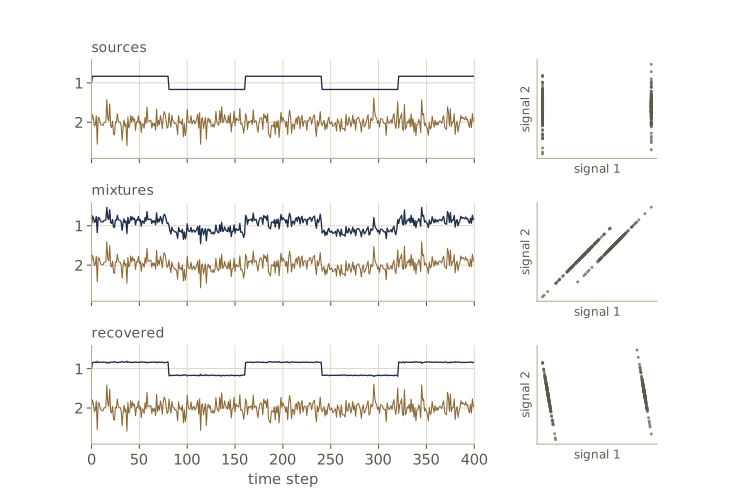
Our two sources are a square wave (lighter tails than a Gaussian) and Laplace noise (heavier tails), both with unit variance, mixed by a matrix we then forget.
def kurtosis(a):
    """Excess kurtosis: 0 for a Gaussian, negative for light tails, positive for heavy tails."""
    a = (a - a.mean()) / a.std()
    return np.mean(a ** 4) - 3

gen_ica = np.random.default_rng(7)
T = 2000
t = np.arange(T)
sources = np.column_stack([np.sign(np.sin(2 * np.pi * t / 160)),          # square wave
                           gen_ica.laplace(0, 1 / np.sqrt(2), T)])         # Laplace, variance 1
A_mix = np.array([[1.0, 0.7], [0.5, 1.0]])
X_mix = sources @ A_mix.T                                   # what the microphones record

def fastica(Y, K, gen, max_iter=200, tol=1e-10):
    """K independent directions (rows) in whitened data Y, found one at a time with deflation."""
    W_ica = np.zeros((K, Y.shape[1]))
    for k in range(K):
        w = gen.standard_normal(Y.shape[1])
        w /= np.linalg.norm(w)
        for it in range(max_iter):
            a = Y @ w
            w_new = np.mean(Y * np.tanh(a)[:, None], axis=0) - np.mean(1 - np.tanh(a) ** 2) * w
            w_new -= W_ica[:k].T @ (W_ica[:k] @ w_new)          # stay orthogonal to earlier rows
            w_new /= np.linalg.norm(w_new)
            converged = abs(abs(w_new @ w) - 1) < tol
            w = w_new
            if converged:
                break
        print(f"component {k + 1}: converged after {it + 1} iterations")
        W_ica[k] = w
    return W_ica

xbar_mix, lam_mix, U_mix = pca_eig(X_mix)
Y_mix = whiten(X_mix, xbar_mix, lam_mix, U_mix)
W_ica = fastica(Y_mix, 2, gen_ica)
recovered = Y_mix @ W_ica.T
print("correlation of recovered components (rows) with true sources (columns):")
print(np.corrcoef(recovered.T, sources.T)[:2, 2:])
print("excess kurtosis  sources:", [f"{kurtosis(s):.3f}" for s in sources.T],
      " mixtures:", [f"{kurtosis(x):.3f}" for x in X_mix.T],
      " recovered:", [f"{kurtosis(r):.3f}" for r in recovered.T])
component 1: converged after 3 iterations
component 2: converged after 2 iterations
correlation of recovered components (rows) with true sources (columns):
[[ 0.0427  0.9981]
 [-0.9991  0.0615]]
excess kurtosis  sources: ['-1.994', '2.122']  mixtures: ['-0.637', '1.427']  recovered: ['2.142', '-1.987']
Each recovered component matches one source with a correlation of magnitude close to 1 (the order and signs are arbitrary, as promised), and the mixtures are visibly closer to Gaussian than the sources: their kurtoses are pulled toward zero. FastICA converges in a handful of iterations because each step is a Newton step. The next cell shows the Gaussian failure case: along every direction of whitened Gaussian mixtures the kurtosis is zero up to sampling noise, so there is nothing to find, while for our sources it swings between the two sources’ values.
G_mix = gen_ica.standard_normal((T, 2)) @ A_mix.T                          # Gaussian sources, mixed
_, lam_g2, U_g2 = pca_eig(G_mix)
Y_gauss = whiten(G_mix, G_mix.mean(axis=0), lam_g2, U_g2)
for name, Y in [("Gaussian sources", Y_gauss), ("our sources     ", Y_mix)]:
    k = [kurtosis(Y @ np.array([np.cos(a), np.sin(a)])) for a in np.linspace(0, np.pi, 7)[:-1]]
    print(name, "kurtosis along directions 0, 30, ..., 150 deg:", np.round(k, 3))
Gaussian sources kurtosis along directions 0, 30, ..., 150 deg: [-0.046  0.029 -0.008 -0.134 -0.111 -0.06 ]
our sources      kurtosis along directions 0, 30, ..., 150 deg: [ 0.322  2.014  1.647 -0.224 -1.806 -1.626]
ICA has many variants, for instance independent factor analysis, which allows noise, different numbers of latent and observed variables, and mixture-of-Gaussians source densities fitted by EM; Intro to ML, module 12 writes down the maximum likelihood version through the change-of-variables formula and runs FastICA on a different pair of signals.
Kalman filters
All the models so far treat data points as independent. For a time series, the natural extension links the latent variables of successive points into a Markov chain, the same graph as a hidden Markov model but with continuous states. With linear-Gaussian conditionals this is the linear dynamical system:
\[p(\mathbf{z}_n \mid \mathbf{z}_{n-1}) = \mathcal{N}(\mathbf{z}_n \mid \mathbf{A}\mathbf{z}_{n-1}, \boldsymbol{\Gamma}), \qquad p(\mathbf{x}_n \mid \mathbf{z}_n) = \mathcal{N}(\mathbf{x}_n \mid \mathbf{C}\mathbf{z}_n, \boldsymbol{\Sigma}), \qquad p(\mathbf{z}_1) = \mathcal{N}(\mathbf{z}_1 \mid \boldsymbol{\mu}_0, \mathbf{V}_0).\]Each emission \(p(\mathbf{x}_n \mid \mathbf{z}_n)\) is a linear-Gaussian latent-variable model like PPCA; what is new is that the latent state drifts according to the dynamics \(\mathbf{A}\) with process noise \(\boldsymbol{\Gamma}\). The parameters are shared across time, so their number does not grow with the length of the sequence. The Kalman filter is the algorithm that computes \(p(\mathbf{z}_n \mid \mathbf{x}_1, \dots, \mathbf{x}_n)\) recursively. Because everything is jointly Gaussian, that distribution stays Gaussian, \(\mathcal{N}(\mathbf{z}_n \mid \boldsymbol{\mu}_n, \mathbf{V}_n)\), and each step is two applications of the Gaussian identities:
- Predict. Push the last estimate through the dynamics: \(\mathbf{P}_{n-1} = \mathbf{A}\mathbf{V}_{n-1}\mathbf{A}^{\mathrm{T}} + \boldsymbol{\Gamma}\), with predicted mean \(\mathbf{A}\boldsymbol{\mu}_{n-1}\).
- Update. Correct the prediction by the new measurement, weighted by the Kalman gain \(\mathbf{K}_n = \mathbf{P}_{n-1}\mathbf{C}^{\mathrm{T}}(\mathbf{C}\mathbf{P}_{n-1}\mathbf{C}^{\mathrm{T}} + \boldsymbol{\Sigma})^{-1}\): \(\boldsymbol{\mu}_n = \mathbf{A}\boldsymbol{\mu}_{n-1} + \mathbf{K}_n(\mathbf{x}_n - \mathbf{C}\mathbf{A}\boldsymbol{\mu}_{n-1})\) and \(\mathbf{V}_n = (\mathbf{I} - \mathbf{K}_n\mathbf{C})\mathbf{P}_{n-1}\).
The gain balances trust in the model against trust in the sensor, and the prediction errors give the log likelihood of the whole sequence as a by-product. The full derivation, a check of the recursion against the joint Gaussian of all states and measurements, the smoother that also uses future measurements, and EM for the parameters are in Intro to ML, module 13.
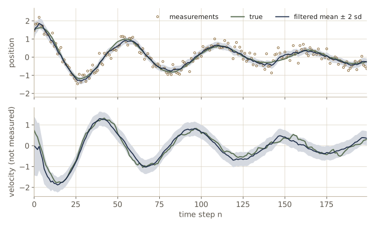
Our example tracks a lightly damped oscillator, a mass on a spring, from noisy readings of its position alone. The state is \(\mathbf{z} = (\text{position}, \text{velocity})\); the dynamics matrix is the exact one-step solution of the spring equation, \(\mathbf{A} = \exp(\mathbf{F}\,\Delta t)\), a matrix exponential; and \(\mathbf{C} = (1, 0)\).
def oscillator(dt=0.1, omega=1.2, zeta=0.08):
    """One-step transition of a damped spring: d/dt (pos, vel) = F (pos, vel)."""
    F = np.array([[0.0, 1.0], [-omega ** 2, -2 * zeta * omega]])
    return linalg.expm(F * dt)

A_kf = oscillator()
Gamma_kf = np.diag([1e-4, 4e-3])                     # small random pushes, mostly on velocity
C_kf = np.array([[1.0, 0.0]])                        # we measure position only
Sigma_kf = np.array([[0.25 ** 2]])                   # sensor noise, standard deviation 0.25
mu0_kf, V0_kf = np.array([1.5, 0.0]), np.diag([0.5, 0.5])

def sample_lds(A, Gamma, C, Sigma, mu0, V0, N, gen):
    Z = np.zeros((N, len(mu0)))
    Z[0] = gen.multivariate_normal(mu0, V0)
    for n in range(1, N):
        Z[n] = gen.multivariate_normal(A @ Z[n - 1], Gamma)
    return Z, Z @ C.T + gen.multivariate_normal(np.zeros(len(C)), Sigma, size=N)

def kalman_filter(X, A, Gamma, C, Sigma, mu0, V0):
    """Filtered means and covariances of p(z_n | x_1..x_n), and ln p(x_1..x_N)."""
    N, L = len(X), len(mu0)
    mus, Vs, loglik = np.zeros((N, L)), np.zeros((N, L, L)), 0.0
    m, P = mu0, V0                                   # prediction for z_1 is the prior
    for n in range(N):
        if n > 0:
            m, P = A @ mus[n - 1], A @ Vs[n - 1] @ A.T + Gamma          # predict
        S_n = C @ P @ C.T + Sigma                                        # predicted cov of x_n
        K = np.linalg.solve(S_n, C @ P).T                                # gain P C^T S_n^-1
        r = X[n] - C @ m                                                 # prediction error
        mus[n], Vs[n] = m + K @ r, (np.eye(L) - K @ C) @ P               # update
        loglik -= 0.5 * (len(r) * np.log(2 * np.pi) + np.linalg.slogdet(S_n)[1]
                         + r @ np.linalg.solve(S_n, r))
    return mus, Vs, loglik

Z_kf, X_kf = sample_lds(A_kf, Gamma_kf, C_kf, Sigma_kf, mu0_kf, V0_kf, 200,
                        np.random.default_rng(12))
mus_kf, Vs_kf, ll_kf = kalman_filter(X_kf, A_kf, Gamma_kf, C_kf, Sigma_kf, mu0_kf, V0_kf)
rms = lambda e: np.sqrt(np.mean(e ** 2))
print(f"RMS position error: raw measurements {rms(X_kf[:, 0] - Z_kf[:, 0]):.4f},"
      f" filtered {rms(mus_kf[:, 0] - Z_kf[:, 0]):.4f}")
print(f"RMS velocity error (never measured): {rms(mus_kf[:, 1] - Z_kf[:, 1]):.4f}")
inside = np.abs(mus_kf[:, 0] - Z_kf[:, 0]) < 2 * np.sqrt(Vs_kf[:, 0, 0])
print(f"true position inside the +-2 sd band: {inside.mean():.1%} of steps")
RMS position error: raw measurements 0.2405, filtered 0.0893
RMS velocity error (never measured): 0.1758
true position inside the +-2 sd band: 97.5% of steps
The filter cuts the position error to well under half of the raw measurement error, recovers a velocity it never observes, and its ±2 sd band contains the true position at 97.5% of the steps, close to the 95% that a well-calibrated Gaussian band should cover.
For the rest of the module we return to independent data points.
The evidence lower bound
In module 15 the evidence lower bound was derived for discrete latent variables. Nothing in the argument needs the latents to be discrete; sums simply become integrals. Take a model \(p(\mathbf{x}, \mathbf{z} \mid \mathbf{w})\) with parameters \(\mathbf{w}\) and any distribution \(q(\mathbf{z})\) over the latent variable. By the product rule, \(\ln p(\mathbf{x} \mid \mathbf{w}) = \ln p(\mathbf{x}, \mathbf{z} \mid \mathbf{w}) - \ln p(\mathbf{z} \mid \mathbf{x}, \mathbf{w})\) for every \(\mathbf{z}\). Add and subtract \(\ln q(\mathbf{z})\) and average both sides over \(q\); the left side does not depend on \(\mathbf{z}\), so
\[\ln p(\mathbf{x} \mid \mathbf{w}) = \mathcal{L}(q, \mathbf{w}) + \mathrm{KL}\left(q(\mathbf{z}) \Vert p(\mathbf{z} \mid \mathbf{x}, \mathbf{w})\right),\]with
\[\mathcal{L}(q, \mathbf{w}) = \int q(\mathbf{z}) \ln\frac{p(\mathbf{x}, \mathbf{z} \mid \mathbf{w})}{q(\mathbf{z})}\,d\mathbf{z}, \qquad \mathrm{KL}\left(q \Vert p\right) = -\int q(\mathbf{z})\ln\frac{p(\mathbf{z} \mid \mathbf{x}, \mathbf{w})}{q(\mathbf{z})}\,d\mathbf{z} .\]The KL divergence is never negative, so \(\mathcal{L}(q, \mathbf{w}) \le \ln p(\mathbf{x} \mid \mathbf{w})\): the evidence lower bound (ELBO), with equality exactly when \(q\) is the posterior. For \(N\) independent data points each gets its own \(q(\mathbf{z}_n)\) and the bound is the sum \(\mathcal{L} = \sum_n \int q(\mathbf{z}_n)\ln\{p(\mathbf{x}_n, \mathbf{z}_n \mid \mathbf{w})/q(\mathbf{z}_n)\}\,d\mathbf{z}_n\).
For PPCA every term is available in closed form when \(q(\mathbf{z}) = \mathcal{N}(\mathbf{z} \mid \mathbf{m}, \mathbf{V})\) is Gaussian, because expectations of quadratics under a Gaussian are easy: \(\mathbb{E}_q[\lVert \mathbf{x} - \mathbf{W}\mathbf{z} - \boldsymbol{\mu} \rVert^2] = \lVert \mathbf{x} - \mathbf{W}\mathbf{m} - \boldsymbol{\mu} \rVert^2 + \operatorname{Tr}(\mathbf{W}^{\mathrm{T}}\mathbf{W}\mathbf{V})\). The next cell checks the decomposition on the toy model for an arbitrary \(q\) and for the exact posterior.
def kl_gauss(m1, V1, m2, V2):
    """KL( N(m1, V1) || N(m2, V2) )."""
    k = len(m1)
    d = m2 - m1
    return 0.5 * (np.trace(np.linalg.solve(V2, V1)) + d @ np.linalg.solve(V2, d) - k
                  + np.linalg.slogdet(V2)[1] - np.linalg.slogdet(V1)[1])

def elbo_ppca(x, m, V, W, mu, sigma2):
    """L(q) = E_q[ln p(x|z)] + E_q[ln p(z)] + entropy of q, for q = N(m, V)."""
    D, M = W.shape
    r = x - W @ m - mu
    e_lik = -0.5 * D * np.log(2 * np.pi * sigma2) - (r @ r + np.trace(W.T @ W @ V)) / (2 * sigma2)
    e_prior = -0.5 * M * np.log(2 * np.pi) - 0.5 * (m @ m + np.trace(V))
    entropy = 0.5 * np.linalg.slogdet(2 * np.pi * np.e * V)[1]
    return e_lik + e_prior + entropy

x0 = X_toy[0]
log_px = gauss_loglik(x0[None, :], mu_toy, C_toy)
post_m = np.linalg.solve(Mm_toy, W_toy.T @ (x0 - mu_toy))
post_V = s2_toy * np.linalg.inv(Mm_toy)
q_m, q_V = np.array([0.5, -1.0]), np.array([[0.3, 0.1], [0.1, 0.2]])      # an arbitrary q
L_q = elbo_ppca(x0, q_m, q_V, W_toy, mu_toy, s2_toy)
print(f"ln p(x) = {log_px:.6f}")
print(f"arbitrary q: ELBO {L_q:.6f} + KL {kl_gauss(q_m, q_V, post_m, post_V):.6f}"
      f" = {L_q + kl_gauss(q_m, q_V, post_m, post_V):.6f}")
print(f"posterior q: ELBO {elbo_ppca(x0, post_m, post_V, W_toy, mu_toy, s2_toy):.6f}")
ln p(x) = -8.012076
arbitrary q: ELBO -24.841085 + KL 16.829009 = -8.012076
posterior q: ELBO -8.012076
Note. When the posterior cannot be computed, we can still maximize \(\mathcal{L}\) over a restricted family of distributions \(q\). The variational autoencoder of module 19 does exactly this, with a neural network that outputs the parameters of a Gaussian \(q(\mathbf{z} \mid \mathbf{x})\) for each data point; the
elbo_ppcafunction above is the linear ancestor of its loss.
Expectation maximization
EM climbs the bound by coordinate ascent. In the E step we hold \(\mathbf{w}\) at its current value \(\mathbf{w}^{\text{old}}\) and maximize \(\mathcal{L}\) over \(q\), which sets \(q(\mathbf{z}_n) = p(\mathbf{z}_n \mid \mathbf{x}_n, \mathbf{w}^{\text{old}})\) and makes the bound touch the log likelihood. In the M step we hold \(q\) fixed and maximize \(\mathcal{L}\) over \(\mathbf{w}\); the entropy of \(q\) does not depend on \(\mathbf{w}\), so this means maximizing the expected complete-data log likelihood \(\sum_n \mathbb{E}_{q}[\ln p(\mathbf{x}_n, \mathbf{z}_n \mid \mathbf{w})]\). Each step can only increase \(\mathcal{L}\), and after an E step \(\mathcal{L}\) equals the log likelihood, so the log likelihood never decreases.
Why run an iterative algorithm for PPCA when the maximum is known in closed form? Three reasons. Forming \(\mathbf{S}\) costs \(O(ND^2)\) and eigendecomposing it \(O(D^3)\), while an EM iteration costs \(O(NDM)\), which is much less when \(D\) is large and \(M\) small. EM also handles data with missing entries, by treating them as extra latent variables. And EM extends to models with no closed form, such as factor analysis.
For PPCA, the complete-data log likelihood is a sum of \(\ln p(\mathbf{x}_n \mid \mathbf{z}_n) + \ln p(\mathbf{z}_n)\), a quadratic function of each \(\mathbf{z}_n\), so its expectation needs only the first two posterior moments. With \(\boldsymbol{\mu}\) set to \(\bar{\mathbf{x}}\), the E step computes, from the posterior formula,
\[\mathbb{E}[\mathbf{z}_n] = \mathbf{M}^{-1}\mathbf{W}^{\mathrm{T}}(\mathbf{x}_n - \bar{\mathbf{x}}), \qquad \mathbb{E}[\mathbf{z}_n\mathbf{z}_n^{\mathrm{T}}] = \sigma^2\mathbf{M}^{-1} + \mathbb{E}[\mathbf{z}_n]\,\mathbb{E}[\mathbf{z}_n]^{\mathrm{T}},\]and setting the derivatives of the expected complete-data log likelihood to zero gives the M step,
\[\begin{aligned} \mathbf{W}^{\text{new}} &= \left[\sum_{n=1}^{N}(\mathbf{x}_n - \bar{\mathbf{x}})\,\mathbb{E}[\mathbf{z}_n]^{\mathrm{T}}\right]\left[\sum_{n=1}^{N}\mathbb{E}[\mathbf{z}_n\mathbf{z}_n^{\mathrm{T}}]\right]^{-1}, \\ \sigma^2_{\text{new}} &= \frac{1}{ND}\sum_{n=1}^{N}\left\{ \lVert\mathbf{x}_n - \bar{\mathbf{x}}\rVert^2 - 2\,\mathbb{E}[\mathbf{z}_n]^{\mathrm{T}}\mathbf{W}_{\text{new}}^{\mathrm{T}}(\mathbf{x}_n - \bar{\mathbf{x}}) + \operatorname{Tr}\left(\mathbb{E}[\mathbf{z}_n\mathbf{z}_n^{\mathrm{T}}]\,\mathbf{W}_{\text{new}}^{\mathrm{T}}\mathbf{W}_{\text{new}}\right) \right\}. \end{aligned}\]The \(\mathbf{W}\) update is a least-squares regression of the data on the expected latent variables, with the posterior covariance added to the “design” term. Both steps involve only sums over data points, so they can also be run online, one point at a time. We fit \(M = 5\) to the MNIST digits from a random start and compare with the closed form.
def ppca_em(X, M, iters, gen, report=()):
    """EM for probabilistic PCA from a random start; returns W, sigma^2, log-likelihood history."""
    N, D = X.shape
    xbar = X.mean(axis=0)
    Xc = X - xbar
    S = Xc.T @ Xc / N                                  # only used to report the log likelihood
    sum_sq = np.sum(Xc ** 2)
    W, sigma2 = 0.1 * gen.standard_normal((D, M)), 1.0      # columns of length about 2.8
    history = []
    for it in range(1, iters + 1):
        Minv = np.linalg.inv(W.T @ W + sigma2 * np.eye(M))        # M x M only
        Ez = Xc @ (W @ Minv)                                       # E step: rows are E[z_n]
        sum_Ezz = N * sigma2 * Minv + Ez.T @ Ez                    # sum_n E[z_n z_n^T]
        W = np.linalg.solve(sum_Ezz, Ez.T @ Xc).T                  # M step for W
        sigma2 = (sum_sq - 2 * np.sum(Ez * (Xc @ W))
                  + np.trace(sum_Ezz @ W.T @ W)) / (N * D)         # M step for sigma^2
        history.append(ppca_loglik(S, N, W, sigma2) / N)
        if it in report:
            print(f"iteration {it:4d}: log likelihood per point {history[-1]:9.4f},"
                  f" sigma^2 {sigma2:.5f}")
    return W, sigma2, np.array(history)

M = 5
W_em, s2_em, hist_em = ppca_em(X, M, 250, np.random.default_rng(0), report=(1, 2, 5, 10, 50, 250))
print("never decreased:", bool(np.all(np.diff(hist_em) > -1e-9)))
W_cf, s2_cf = ppca_ml(lam, U, M)
print(f"closed form:    log likelihood per point {ppca_loglik(S, N, W_cf, s2_cf) / N:9.4f},"
      f" sigma^2 {s2_cf:.5f}")
print(f"largest principal angle to the closed-form subspace: "
      f"{np.degrees(linalg.subspace_angles(W_em, W_cf).max()):.4f} deg")
iteration    1: log likelihood per point   27.6672, sigma^2 0.06669
iteration    2: log likelihood per point   64.4579, sigma^2 0.04921
iteration    5: log likelihood per point   87.3876, sigma^2 0.04559
iteration   10: log likelihood per point   91.9245, sigma^2 0.04492
iteration   50: log likelihood per point   93.1378, sigma^2 0.04490
iteration  250: log likelihood per point   93.2098, sigma^2 0.04490
never decreased: True
closed form:    log likelihood per point   93.2099, sigma^2 0.04490
largest principal angle to the closed-form subspace: 0.0000 deg
The log likelihood never decreases and approaches the closed-form maximum, and \(\sigma^2\) settles within about ten iterations. Most of the gain comes in the first few iterations; the slow tail that follows, in which \(\mathbf{W}\) keeps turning toward the principal subspace and its columns grow to their final lengths, is typical of EM. Its speed depends on the ratios between successive eigenvalues, which are close to 1 for MNIST. After 250 iterations the subspace agrees with the leading eigenvectors to well under a thousandth of a degree.
The scale of the random start matters more than one might expect. Suppose \(\mathbf{W}\) points along an eigenvector \(\mathbf{u}_i\) but is far too long. Working through the two steps for this case shows that each iteration shrinks it only by the factor \(\lambda_i/(\lambda_i + \sigma^2)\), about 0.99 here. Starting from standard normal entries (columns of length about 28, against a final length of at most \(\sqrt{\lambda_1 - \sigma^2} \approx 2.3\)) therefore costs hundreds of extra iterations, which is why the code scales the start down.
EM for PCA
EM survives the limit \(\sigma^2 \to 0\), where PPCA becomes ordinary PCA. Then \(\mathbf{M} \to \mathbf{W}^{\mathrm{T}}\mathbf{W}\), the posterior covariance vanishes, and only \(\mathbb{E}[\mathbf{z}_n]\) is needed. Collect the centered data in the \(N \times D\) matrix \(\tilde{\mathbf{X}}\) and the expected latent vectors as the columns of an \(M \times N\) matrix \(\boldsymbol{\Omega}\). The two steps become
\[\boldsymbol{\Omega} = \left(\mathbf{W}_{\text{old}}^{\mathrm{T}}\mathbf{W}_{\text{old}}\right)^{-1}\mathbf{W}_{\text{old}}^{\mathrm{T}}\tilde{\mathbf{X}}^{\mathrm{T}}, \qquad \mathbf{W}_{\text{new}} = \tilde{\mathbf{X}}^{\mathrm{T}}\boldsymbol{\Omega}^{\mathrm{T}}\left(\boldsymbol{\Omega}\boldsymbol{\Omega}^{\mathrm{T}}\right)^{-1}.\]Both are least-squares problems for the same reconstruction error \(\sum_n \lVert \mathbf{x}_n - \bar{\mathbf{x}} - \mathbf{W}\mathbf{z}_n \rVert^2\). The E step fixes the subspace and finds each point’s coordinates by orthogonal projection; the M step fixes the coordinates and moves the subspace to fit them best. A mechanical picture for \(D = 2\) and \(M = 1\): the subspace is a rigid rod through the mean and each data point is tied to it by a spring. First the attachment points slide along the fixed rod until every spring is as short as possible (the E step); then they are clamped and the rod swings to the position of least total spring energy (the M step). Alternating the two never increases the energy, and the rod settles on the principal axis.
def pca_em(X, M, iters, gen, U_ref, report=()):
    """Zero-noise EM for PCA; prints the largest principal angle to span(U_ref)."""
    Xc = X - X.mean(axis=0)
    W = gen.standard_normal((X.shape[1], M))
    for it in range(1, iters + 1):
        Omega = np.linalg.solve(W.T @ W, W.T @ Xc.T)           # E step: project onto span(W)
        W = np.linalg.solve(Omega @ Omega.T, Omega @ Xc).T     # M step: refit the subspace
        if it in report:
            angle = np.degrees(linalg.subspace_angles(W, U_ref).max())
            print(f"iteration {it:4d}: largest principal angle {angle:8.4f} deg")
    return W

W_pca_em = pca_em(X, 5, 300, np.random.default_rng(1), U[:, :5], report=(1, 5, 20, 50, 100, 300))
Q_em = np.linalg.qr(W_pca_em)[0]                                # orthonormal basis of span(W)
lam_em = np.linalg.eigvalsh(Q_em.T @ S @ Q_em)[::-1]            # eigenvalues inside the subspace
print("eigenvalues recovered from the EM subspace:", lam_em)
print("leading eigenvalues of S:                  ", lam[:5])
iteration    1: largest principal angle  71.9487 deg
iteration    5: largest principal angle  39.9164 deg
iteration   20: largest principal angle  17.0945 deg
iteration   50: largest principal angle   3.3890 deg
iteration  100: largest principal angle   0.2184 deg
iteration  300: largest principal angle   0.0000 deg
eigenvalues recovered from the EM subspace: [5.3047 3.8764 3.2865 2.9121 2.4859]
leading eigenvalues of S:                   [5.3047 3.8764 3.2865 2.9121 2.4859]
The principal angles between two \(M\)-dimensional subspaces are the angles between their best-aligned orthonormal bases; the largest one is zero only if the subspaces coincide. EM converges to the principal subspace, not to the eigenvectors themselves: the columns of \(\mathbf{W}\) are an arbitrary basis of it. A small \(M \times M\) eigenproblem inside the subspace, as in the last two lines, recovers the individual directions and eigenvalues. The cost per iteration is \(O(NDM)\), and \(\mathbf{S}\) is never formed (we used it above only to compare).
EM for factor analysis
Factor analysis has no closed-form maximum likelihood solution, so EM is the standard way to fit it. The derivation mirrors PPCA with \(\sigma^2\mathbf{I}\) replaced by \(\boldsymbol{\Psi}\). The E step uses
\[\mathbf{G} = \left(\mathbf{I} + \mathbf{W}^{\mathrm{T}}\boldsymbol{\Psi}^{-1}\mathbf{W}\right)^{-1}, \qquad \mathbb{E}[\mathbf{z}_n] = \mathbf{G}\mathbf{W}^{\mathrm{T}}\boldsymbol{\Psi}^{-1}(\mathbf{x}_n - \bar{\mathbf{x}}), \qquad \mathbb{E}[\mathbf{z}_n\mathbf{z}_n^{\mathrm{T}}] = \mathbf{G} + \mathbb{E}[\mathbf{z}_n]\,\mathbb{E}[\mathbf{z}_n]^{\mathrm{T}},\]which again inverts only \(M \times M\) matrices (\(\boldsymbol{\Psi}\) is diagonal). The M step updates \(\mathbf{W}\) exactly as for PPCA and sets each uniqueness to the part of that variable’s variance the factors do not explain:
\[\boldsymbol{\Psi}^{\text{new}} = \operatorname{diag}\left\{ \mathbf{S} - \mathbf{W}^{\text{new}}\,\frac{1}{N}\sum_{n=1}^{N}\mathbb{E}[\mathbf{z}_n](\mathbf{x}_n - \bar{\mathbf{x}})^{\mathrm{T}} \right\},\]where \(\operatorname{diag}\) keeps the diagonal and zeroes the rest. Back to the six sensors:
def fa_em(X, M, iters, gen):
    """EM for factor analysis; returns mean, loadings W, uniquenesses psi, log-lik. history."""
    N, D = X.shape
    xbar = X.mean(axis=0)
    Xc = X - xbar
    S = Xc.T @ Xc / N
    W, psi = gen.standard_normal((D, M)), np.diag(S).copy()
    history = []
    for it in range(iters):
        G = np.linalg.inv(np.eye(M) + (W.T / psi) @ W)
        Ez = Xc @ (W / psi[:, None]) @ G                          # E step: rows are E[z_n]
        sum_Ezz = N * G + Ez.T @ Ez
        W = np.linalg.solve(sum_Ezz, Ez.T @ Xc).T                 # M step for W
        psi = np.diag(S - W @ (Ez.T @ Xc) / N).copy()             # M step for Psi
        history.append(gauss_loglik(X, xbar, W @ W.T + np.diag(psi)) / N)
    return xbar, W, psi, np.array(history)

xbar_fa, W_fa, psi_fa, hist_fa = fa_em(X_fa, 2, 300, np.random.default_rng(0))
print("log likelihood per point, iterations 1-5:", np.round(hist_fa[:5], 4),
      " final:", f"{hist_fa[-1]:.4f}")
print("never decreased:", bool(np.all(np.diff(hist_fa) > -1e-12)))
print("uniquenesses:", psi_fa, "\ntrue values:  ", psi_true)
print("principal angles to the true subspace (deg):",
      np.degrees(linalg.subspace_angles(W_fa, W_fa_true)))
C_fa = W_fa @ W_fa.T + np.diag(psi_fa)
C_pp = W_pp @ W_pp.T + s2_pp * np.eye(6)
print(f"held-out log likelihood per point: factor analysis"
      f" {gauss_loglik(X_fa_test, xbar_fa, C_fa) / 1000:.4f},"
      f" PPCA {gauss_loglik(X_fa_test, xbar_fa, C_pp) / 1000:.4f}")
log likelihood per point, iterations 1-5: [-9.1878 -8.5567 -8.0834 -7.7905 -7.6457]  final: -7.5222
never decreased: True
uniquenesses: [0.0685 0.0889 0.0969 0.2812 1.0768 3.1933]
true values:   [0.05 0.1  0.1  0.3  1.   3.  ]
principal angles to the true subspace (deg): [2.5252 1.1377]
held-out log likelihood per point: factor analysis -7.4251, PPCA -8.8625
Factor analysis recovers the six noise levels, finds the true subspace to within a few degrees, and beats PPCA clearly on held-out data. The last check is the rescaling property: multiply the first sensor’s readings by 10 and refit.
scale = np.array([10.0, 1, 1, 1, 1, 1])
_, W_fa10, psi_fa10, _ = fa_em(X_fa * scale, 2, 300, np.random.default_rng(0))
print("uniquenesses after / before rescaling:", psi_fa10 / psi_fa)
WWt_pred = (scale[:, None] * W_fa) @ (scale[:, None] * W_fa).T      # rescaled rows of W, then W W^T
print(f"max |W W^T after - predicted|: {np.max(np.abs(W_fa10 @ W_fa10.T - WWt_pred)):.1e}")
uniquenesses after / before rescaling: [100.   1.   1.   1.   1.   1.]
max |W W^T after - predicted|: 3.2e-09
The first uniqueness grows by a factor of \(10^2\) and the others are unchanged, as the covariance argument predicted. The loadings are compared through \(\mathbf{W}\mathbf{W}^{\mathrm{T}}\), which removes the latent rotation: EM started from the same random \(\mathbf{W}\) can end in a different rotation of the same solution.
In practice. Use PPCA (or plain PCA) when the variables are measured on the same scale with similar noise, such as the pixels of an image, and factor analysis when they are heterogeneous measurements whose noise levels differ. Both are cheap enough to try as baselines before any deep generative model: if a linear-Gaussian model with a handful of latent dimensions explains the data well, a deep model has little left to add.
Nonlinear latent-variable models
The linear models above can only describe data near a flat subspace, and the MNIST spectrum shows that digits are not like that: a flat subspace needs hundreds of dimensions to reach 99% of the variance, far more than the handful of ways a digit can actually vary. The natural generalization keeps the simple latent distribution and replaces the linear map by a deep network \(\mathbf{g}(\mathbf{z}, \mathbf{w})\) with weights and biases \(\mathbf{w}\):
\[p_{\mathbf{z}}(\mathbf{z}) = \mathcal{N}(\mathbf{z} \mid \mathbf{0}, \mathbf{I}), \qquad \mathbf{x} = \mathbf{g}(\mathbf{z}, \mathbf{w}) .\]Sampling is as easy as for PPCA: draw \(\mathbf{z}\) and run the network forward, with no iteration. Learning is the hard part. If \(\mathbf{g}\) were invertible, with inverse \(\mathbf{z}(\mathbf{x})\), the density of \(\mathbf{x}\) would follow from the change-of-variables formula of module 02,
\[p_{\mathbf{x}}(\mathbf{x}) = p_{\mathbf{z}}(\mathbf{z}(\mathbf{x}))\,\left\lvert \det \mathbf{J}(\mathbf{x}) \right\rvert, \qquad J_{ij}(\mathbf{x}) = \frac{\partial z_i}{\partial x_j} .\]But an ordinary network has no inverse: it may map many inputs to the same output, and if \(\mathbf{z}\) has fewer dimensions than \(\mathbf{x}\) it cannot be invertible at all. Restricting to invertible networks with \(\dim\mathbf{z} = \dim\mathbf{x}\) is one way forward, the normalizing flows of module 18. This section looks at the other case.
Nonlinear manifolds
Let the latent space have dimension \(M < D\). Then the network’s outputs \(\mathbf{g}(\mathbf{z}, \mathbf{w})\) trace out an \(M\)-dimensional curved surface in data space, and all samples lie exactly on it. That is a strong and often correct inductive bias: natural images do not fill pixel space. It also causes a problem for learning. A distribution concentrated on a surface assigns zero density to every point off it, and a real data point will essentially never lie exactly on the surface, so the likelihood is zero for every \(\mathbf{w}\) and gives no gradient to follow.
The fix is the one we used for regression networks: let the network output the parameters of a distribution defined on the whole data space. For continuous data,
\[p(\mathbf{x} \mid \mathbf{z}, \mathbf{w}) = \mathcal{N}\left(\mathbf{x} \mid \mathbf{g}(\mathbf{z}, \mathbf{w}), \sigma^2\mathbf{I}\right),\]with linear output units so that \(\mathbf{g} \in \mathbb{R}^D\). PPCA is the special case \(\mathbf{g}(\mathbf{z}, \mathbf{w}) = \mathbf{W}\mathbf{z} + \boldsymbol{\mu}\). Sampling now has three steps: draw \(\mathbf{z}\) from the prior, run the network, and add Gaussian noise. The marginal distribution of the data is
\[p(\mathbf{x} \mid \mathbf{w}) = \int p(\mathbf{x} \mid \mathbf{z}, \mathbf{w})\,p(\mathbf{z})\,d\mathbf{z} .\]To see such a model we take \(M = 1\) and \(D = 2\), so that everything can be drawn, and use an untrained network with one hidden layer of eight tanh units and random weights. Even an untrained network bends a straight latent line into a curve.
def init_generator(H, gen):
    """Random weights of a 1 -> H -> 2 tanh network (not trained: any network defines a model)."""
    return (gen.normal(0, 1.5, H), gen.normal(0, 1.0, H),
            gen.normal(0, 1.5 / np.sqrt(H), (H, 2)), np.zeros(2))

def g(z, w):
    """Network output g(z, w) for a batch of scalar latents z; rows are points in R^2."""
    W1, b1, W2, b2 = w
    return np.tanh(z[:, None] * W1 + b1) @ W2 + b2

w_gen = init_generator(8, np.random.default_rng(21))
sigma = 0.1

def sample_nonlinear(N, w, sigma, gen):
    """z ~ N(0, 1), then x ~ N(g(z, w), sigma^2 I)."""
    z = gen.standard_normal(N)
    return g(z, w) + sigma * gen.standard_normal((N, 2)), z

X_nl, z_nl = sample_nonlinear(500, w_gen, sigma, np.random.default_rng(160))
print("g(z) at z = -2, -1, 0, 1, 2:\n", g(np.linspace(-2, 2, 5), w_gen))
print("first samples x:\n", X_nl[:3])
g(z) at z = -2, -1, 0, 1, 2:
 [[ 0.283  -1.1911]
 [ 0.3918 -1.8495]
 [-0.8608 -0.943 ]
 [-1.2271 -0.1675]
 [-0.4755 -0.0007]]
first samples x:
 [[ 0.3383 -1.5811]
 [-1.3462 -0.3914]
 [ 0.2583 -1.7886]]
The likelihood function
The integral for \(p(\mathbf{x} \mid \mathbf{w})\) contains two Gaussians, but the mean of one of them is a nonlinear function of the integration variable, so there is no closed form. With a one-dimensional latent we can still compute it accurately by quadrature, summing the integrand over a fine grid of \(z\) values; this gives us a reference to measure approximations against. In a realistic model, with tens or hundreds of latent dimensions, a grid is out of the question.
The obvious approximation replaces the integral by an average over samples from the prior,
\[p(\mathbf{x} \mid \mathbf{w}) \approx \frac{1}{K}\sum_{k=1}^{K} p(\mathbf{x} \mid \mathbf{z}_k, \mathbf{w}), \qquad \mathbf{z}_k \sim p(\mathbf{z}),\]which turns the model into a mixture of \(K\) Gaussians with equal weights. It is exact as \(K \to \infty\). We evaluate both in log space with log-sum-exp.
def log_gauss_iso(X, Mu, s):
    """ln N(x_p | mu_k, s^2 I) in 2-D for every pair: rows of X (P) against rows of Mu (K)."""
    d2 = np.sum((X[:, None, :] - Mu[None, :, :]) ** 2, axis=-1)
    return -d2 / (2 * s ** 2) - np.log(2 * np.pi * s ** 2)

z_grid = np.linspace(-6, 6, 2401)                  # quadrature grid for the 1-D latent
dz = z_grid[1] - z_grid[0]
log_pz_grid = -0.5 * z_grid ** 2 - 0.5 * np.log(2 * np.pi)
g_grid = g(z_grid, w_gen)

def log_px_quad(X, s, chunk=1000):
    """ln p(x) = ln integral N(x | g(z), s^2 I) N(z | 0, 1) dz, by a Riemann sum on z_grid."""
    return np.concatenate([logsumexp(log_gauss_iso(X[i:i + chunk], g_grid, s) + log_pz_grid, axis=1)
                           for i in range(0, len(X), chunk)]) + np.log(dz)

def log_px_mc(X, s, K, gen):
    """ln of the average of p(x | z_k) over K samples z_k from the prior."""
    z = gen.standard_normal(K)
    return logsumexp(log_gauss_iso(X, g(z, w_gen), s), axis=1) - np.log(K)

ref = log_px_quad(X_nl, sigma)
print(f"quadrature: mean log likelihood {ref.mean():.4f}")
xx, yy = np.meshgrid(np.linspace(-3, 2, 101), np.linspace(-3, 1.5, 91))
grid_pts = np.column_stack([xx.ravel(), yy.ravel()])
mass = np.exp(log_px_quad(grid_pts, sigma)).sum() * (5 / 100) * (4.5 / 90)
print(f"density integrates to {mass:.4f} over the plotting window")
for K in [10, 100, 1000, 10000]:
    est = log_px_mc(X_nl, sigma, K, np.random.default_rng(K))
    print(f"K = {K:5d} prior samples: mean log likelihood {est.mean():.4f}")
quadrature: mean log likelihood -0.5376
density integrates to 1.0000 over the plotting window
K =    10 prior samples: mean log likelihood -4.0429
K =   100 prior samples: mean log likelihood -0.5793
K =  1000 prior samples: mean log likelihood -0.5461
K = 10000 prior samples: mean log likelihood -0.5400
With a few thousand samples per data point the estimate is close, in this toy problem. Note that the estimated log likelihood is too low for small \(K\), and not just noisy: the average of \(p(\mathbf{x} \mid \mathbf{z}_k)\) is unbiased, but its logarithm is biased downward because \(\ln\) is concave (Jensen’s inequality). Most of the \(\mathbf{z}_k\) land at places on the curve far from \(\mathbf{x}\) and contribute almost nothing; the estimate depends on the few that happen to land nearby.
How few? A prior sample is useful only if \(\mathbf{g}(\mathbf{z}_k)\) lands within a few \(\sigma\) of \(\mathbf{x}\), so the fraction of useful samples shrinks in proportion to \(\sigma\) for a one-dimensional latent, and like \(\sigma^M\) for an \(M\)-dimensional one. The next cell measures the relative spread of the \(K = 100\) estimate at one point near the curve as \(\sigma\) shrinks.
x_on = g(np.array([0.3]), w_gen)                       # a point on the curve
print("  sigma   p(x)    rel. std of estimate (K = 100)   useful fraction of prior samples")
for s in [0.3, 0.1, 0.03, 0.01]:
    x_test = x_on + 0.5 * s                            # a typical offset, about 0.7 sigma
    p_ref = np.exp(log_px_quad(x_test, s))[0]
    gen = np.random.default_rng(1)
    est = np.array([np.exp(log_px_mc(x_test, s, 100, gen))[0] for _ in range(300)])
    near = np.sum((g(gen.standard_normal(100_000), w_gen) - x_test) ** 2, axis=1) < (3 * s) ** 2
    print(f"  {s:5.2f}  {p_ref:7.3f}   {est.std() / p_ref:10.3f}"
          f"                       {near.mean():.4f}")
  sigma   p(x)    rel. std of estimate (K = 100)   useful fraction of prior samples
   0.30    0.444        0.112                       0.5698
   0.10    1.101        0.259                       0.2152
   0.03    3.479        0.496                       0.0596
   0.01   10.332        0.945                       0.0198
The useful fraction falls roughly in proportion to \(\sigma\) (about tenfold between \(\sigma = 0.1\) and \(0.01\)), and the relative spread of the estimate grows until, at \(\sigma = 0.01\), it is about as large as the value being estimated. Now picture images. The latent space has tens of dimensions, and a good model needs a small \(\sigma\), because pixel-level noise of large variance would blur every sample. The useful fraction is then astronomically small.
Worse, Euclidean closeness in pixel space is a poor guide to what “nearby” should mean. Bishop & Bishop §16.4.2 makes this point with a figure borrowed from Doersch’s tutorial (see Going further); here is our own version. Compare an MNIST digit with a copy shifted one pixel to the right, and with a copy that has a small patch of its stroke erased:
digit = X[0].reshape(28, 28)
shifted = np.roll(digit, 1, axis=1)                    # the same digit, one pixel to the right
erased = digit.copy()
erased[14:18, 14:18] = 0                               # a 4 x 4 hole in the stroke
print(f"squared distance to the shifted copy: {np.sum((digit - shifted) ** 2):.2f}")
print(f"squared distance to the damaged copy: {np.sum((digit - erased) ** 2):.2f}")
squared distance to the shifted copy: 20.81
squared distance to the damaged copy: 7.67
The shifted digit is a perfectly good example of the same digit, and the damaged one is not, yet the damaged one is much closer. Under a Gaussian \(p(\mathbf{x} \mid \mathbf{z})\), a value of \(\sigma\) small enough to give the damaged copy a low likelihood gives the shifted one an even lower one. To estimate the likelihood of a digit by sampling from the prior, we would have to wait for a \(\mathbf{z}\) whose output matches the digit almost pixel for pixel, which essentially never happens.
The way out is to sample \(\mathbf{z}\) not from the prior but from a distribution concentrated where the posterior \(p(\mathbf{z} \mid \mathbf{x})\) is, and to correct with importance weights (module 14):
\[p(\mathbf{x} \mid \mathbf{w}) \approx \frac{1}{K}\sum_{k=1}^{K} \frac{p(\mathbf{x} \mid \mathbf{z}_k, \mathbf{w})\,p(\mathbf{z}_k)}{q(\mathbf{z}_k \mid \mathbf{x})}, \qquad \mathbf{z}_k \sim q(\mathbf{z} \mid \mathbf{x}) .\]Here we cheat to build \(q\): we find the grid point \(z^\star\) whose output is closest to \(\mathbf{x}\) and use a Gaussian around it whose width comes from the local slope of the curve. A variational autoencoder learns a network, the encoder, to produce such a \(q\) for any \(\mathbf{x}\) in one forward pass.
def log_px_importance(x, s, K, gen):
    """Importance-sampling estimate of ln p(x) with a Gaussian proposal near the posterior."""
    z_star = z_grid[np.argmin(np.sum((g_grid - x) ** 2, axis=1))]
    slope = (g(np.array([z_star + 1e-5]), w_gen) - g(np.array([z_star - 1e-5]), w_gen)) / 2e-5
    s_q = s / np.linalg.norm(slope)                    # width of the posterior along the curve
    z = z_star + s_q * gen.standard_normal(K)
    log_q = -0.5 * ((z - z_star) / s_q) ** 2 - np.log(s_q * np.sqrt(2 * np.pi))
    log_w = log_gauss_iso(x, g(z, w_gen), s)[0] - 0.5 * z ** 2 - 0.5 * np.log(2 * np.pi) - log_q
    return logsumexp(log_w) - np.log(K)

for s in [0.1, 0.01]:
    x_test = x_on + 0.5 * s
    p_ref = np.exp(log_px_quad(x_test, s))[0]
    gen = np.random.default_rng(2)
    est = np.array([np.exp(log_px_importance(x_test, s, 10, gen)) for _ in range(300)])
    print(f"sigma = {s:4.2f}: relative std with K = 10 importance samples {est.std() / p_ref:.4f}")
sigma = 0.10: relative std with K = 10 importance samples 0.1565
sigma = 0.01: relative std with K = 10 importance samples 0.0132
Ten well-placed samples already beat a hundred prior samples at \(\sigma = 0.1\), and at \(\sigma = 0.01\), where prior sampling was nearly useless, they give about 1% accuracy. The smaller the noise, the more sharply peaked and nearly Gaussian the posterior is, and the better a Gaussian proposal fits it.
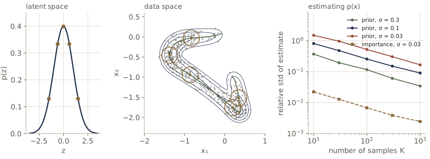
Discrete data
For binary data, such as black-and-white images, the Gaussian output distribution is replaced by a product of Bernoulli distributions whose means come from sigmoid output units:
\[p(\mathbf{x} \mid \mathbf{z}, \mathbf{w}) = \prod_{i=1}^{D} g_i(\mathbf{z}, \mathbf{w})^{x_i}\left(1 - g_i(\mathbf{z}, \mathbf{w})\right)^{1 - x_i}, \qquad g_i = \sigma(a_i(\mathbf{z}, \mathbf{w})),\]where \(a_i\) is the pre-activation of output unit \(i\). For a one-hot categorical variable we use a softmax over the output pre-activations, \(p(\mathbf{x} \mid \mathbf{z}, \mathbf{w}) = \prod_i g_i^{x_i}\) with \(g_i = \exp(a_i)/\sum_j \exp(a_j)\). The negative log likelihoods are the binary and multiclass cross-entropy errors of module 05, and a data vector that mixes variable types gets a product of the matching output distributions.
A subtler problem arises for data that are continuous in spirit but stored as integers, like 8-bit pixel intensities in \(\{0, \dots, 255\}\). A continuous density fitted to integer-valued data can cheat: by piling narrow spikes of density onto the integers it can make the likelihood as large as it likes, without learning anything about the data. Dequantization removes the loophole by adding uniform noise, replacing each integer value \(k\) by \(k + u\) with \(u \sim \mathcal{U}(0, 1)\), so the data fill the space between the integers. Then a density can collect at most the probability \(P(k)\) over the unit interval above \(k\), and the continuous log likelihood of dequantized data is bounded above by the discrete log likelihood of the original values. The next cell shows both effects on 1,000 draws of a variable with six values, fitting a mixture of narrow Gaussians of width \(s\) with one component per value.
gen_dq = np.random.default_rng(5)
probs = np.array([0.05, 0.15, 0.30, 0.25, 0.15, 0.10])
k_vals = gen_dq.choice(6, size=1000, p=probs)                 # integer-valued data
freq = np.bincount(k_vals, minlength=6) / len(k_vals)
k_deq = k_vals + gen_dq.uniform(0, 1, len(k_vals))           # dequantized data

def log_spikes(x, centers, s):
    """Log density of a mixture of Gaussians of width s, weight freq[k], at the given centers."""
    return logsumexp(np.log(freq) - 0.5 * ((x[:, None] - centers) / s) ** 2
                     - np.log(s * np.sqrt(2 * np.pi)), axis=1)

print(f"discrete log likelihood per point: {np.mean(np.log(freq[k_vals])):.4f}")
print("  width s   raw integers   dequantized")
for s in [0.3, 0.1, 0.01, 0.001]:
    raw = np.mean(log_spikes(k_vals.astype(float), np.arange(6), s))
    deq = np.mean(log_spikes(k_deq, np.arange(6) + 0.5, s))
    print(f"  {s:7.3f}  {raw:12.4f}  {deq:12.4f}")
hist = np.mean(np.log(freq[np.floor(k_deq).astype(int)]))    # uniform density P(k) on [k, k+1)
print(f"histogram density on dequantized data: {hist:.4f}")
discrete log likelihood per point: -1.6706
  width s   raw integers   dequantized
    0.300       -1.3785       -1.7134
    0.100       -0.2870       -4.3885
    0.010        2.0156     -409.6817
    0.001        4.3182   -41165.4345
histogram density on dequantized data: -1.6706
On the raw integers the log likelihood grows without limit as the spikes narrow. On the dequantized data narrow spikes are punished, and the best a density can do is the histogram that spreads \(P(k)\) evenly over \([k, k + 1)\), which reaches the discrete log likelihood exactly.
Four approaches to generative modelling
A deep nonlinear latent-variable model is very expressive: networks are universal approximators, so in principle such a model can approximate essentially any distribution, and sampling from it costs one forward pass. Everything difficult is in training, because the likelihood is an integral we cannot compute. The four families of models in the remaining modules can be read as four different ways of dodging that integral, and each pays a different price.
Two properties are worth tracking for each of them. A generative model is one from which we can draw new samples resembling the data; it has a tractable likelihood if \(p(\mathbf{x} \mid \mathbf{w})\) can be evaluated exactly for a given \(\mathbf{x}\), and efficient sampling if a sample takes a single pass through the network.
- Generative adversarial networks (module 17) keep the generator \(\mathbf{g}(\mathbf{z}, \mathbf{w})\) exactly as above, with a latent space smaller than the data space and no inverse, and give up on the likelihood altogether. A second network, the discriminator, is trained to tell real data from generated samples, and its judgment is the training signal for the generator. Samples can be of very high quality and cost one forward pass, but there is no likelihood to monitor or compare, and the two-player training can be unstable.
- Normalizing flows (module 18) take the change-of-variables route: they make the latent space as large as the data space and restrict the network to invertible layers whose Jacobian determinants are cheap. The likelihood is then exact and sampling is efficient, at the price of constrained architectures and no dimensionality reduction.
- Variational autoencoders (module 19) keep the model of this section, including the lower-dimensional latent space and the Gaussian \(p(\mathbf{x} \mid \mathbf{z}, \mathbf{w})\), and train a second network, the encoder, to approximate the posterior \(p(\mathbf{z} \mid \mathbf{x})\). Both networks maximize the ELBO of the last section together. Training is stable and sampling is one pass, but the objective is only a bound, and samples tend to be less sharp than those of the best GANs or diffusion models.
- Diffusion models (module 20) define a long chain of latent variables of the same dimension as the data, obtained by gradually adding noise, and train a network to undo one small step of noise at a time. Each step is an easy learning problem, and the approach gives state-of-the-art results in many applications, but generating a sample takes many passes through the network.
| Approach | Latent dimension | Likelihood | Extra network | Sampling cost | Main price paid |
|---|---|---|---|---|---|
| GAN | \(M < D\) | none | discriminator | one pass | unstable training, no density |
| Normalizing flow | \(M = D\) | exact | none | one pass | invertible architectures only |
| VAE | \(M < D\) | lower bound (ELBO) | encoder \(q(\mathbf{z} \mid \mathbf{x})\) | one pass | approximate posterior, blurrier samples |
| Diffusion model | \(D\) per step, many steps | lower bound | none (one denoiser reused) | many passes | slow sampling |
Note. All four share the recipe of this section: a simple distribution over \(\mathbf{z}\) and a network that transforms it. They differ in what they ask the network to satisfy (invertibility, fooling a critic, matching an encoder, or denoising) so that training becomes possible without the integral \(\int p(\mathbf{x} \mid \mathbf{z}, \mathbf{w})\,p(\mathbf{z})\,d\mathbf{z}\). The linear-Gaussian models of this module are the one case where that integral is easy, which is why they are the reference point for everything that follows.
Summary
| Model | Latent variables and map | Noise | How it is fitted |
|---|---|---|---|
| PCA | \(M\) coordinates, orthogonal projection | none | leading eigenvectors of \(\mathbf{S}\) (SVD of centered data; Gram matrix if \(N < D\)); error \(J = \sum_{i>M}\lambda_i\) |
| Probabilistic PCA | \(\mathbf{z} \sim \mathcal{N}(\mathbf{0}, \mathbf{I})\), \(\mathbf{x} = \mathbf{W}\mathbf{z} + \boldsymbol{\mu} + \boldsymbol{\epsilon}\) | isotropic \(\sigma^2\mathbf{I}\) | closed form \(\mathbf{W} = \mathbf{U}_M(\mathbf{L}_M - \sigma^2\mathbf{I})^{1/2}\mathbf{R}\), or EM |
| Factor analysis | as PPCA | diagonal \(\boldsymbol{\Psi}\) | EM only |
| ICA | \(\mathbf{x} = \mathbf{A}\mathbf{z}\), independent non-Gaussian \(z_j\) | none | whitening + FastICA, or maximum likelihood |
| Linear dynamical system | Markov chain \(\mathbf{z}_n = \mathbf{A}\mathbf{z}_{n-1} +\) noise | Gaussian | Kalman filter for inference; EM for parameters |
| Nonlinear latent-variable model | \(\mathbf{z} \sim \mathcal{N}(\mathbf{0}, \mathbf{I})\), \(\mathbf{x} \sim \mathcal{N}(\mathbf{g}(\mathbf{z}, \mathbf{w}), \sigma^2\mathbf{I})\) | Gaussian, Bernoulli, softmax | likelihood intractable: GANs, flows, VAEs, diffusion |
Ideas to carry forward:
- PCA’s two definitions coincide because kept variance and reconstruction error add up to the fixed total \(\operatorname{Tr}(\mathbf{S})\). The linear encoder–decoder view of PCA is the template for autoencoders.
- A latent-variable model turns a projection into a density. With Gaussian latents and linear maps everything (marginal, posterior, maximum likelihood) is available in closed form, only the subspace is identified, and non-Gaussian latents (ICA) or temporal structure (the Kalman filter) change what can be learned.
- The ELBO \(\ln p(\mathbf{x}) = \mathcal{L}(q, \mathbf{w}) + \mathrm{KL}(q \Vert p(\mathbf{z} \mid \mathbf{x}, \mathbf{w}))\) holds for continuous latents too. EM uses the exact posterior for \(q\); when that is unavailable, a learned \(q\) gives the variational autoencoder.
- With a nonlinear network in place of \(\mathbf{W}\), sampling stays cheap but the likelihood becomes an intractable integral, and naive Monte Carlo over the prior fails badly in high dimensions. The four deep generative families of modules 17–20 are four ways around this.
Exercises
- Complete the induction for the maximum-variance result: assume the best \(M\)-dimensional projection is spanned by \(\mathbf{u}_1, \dots, \mathbf{u}_M\), introduce Lagrange multipliers for unit length and for orthogonality to each earlier direction, and show that the best new direction is the eigenvector with the \((M+1)\)-th largest eigenvalue. Where do you use that \(\mathbf{S}\) is symmetric?
- Show that if \(\mathbf{v}_i\) is a unit eigenvector of the Gram matrix \(\frac{1}{N}\tilde{\mathbf{X}}\tilde{\mathbf{X}}^{\mathrm{T}}\) with eigenvalue \(\lambda_i > 0\), then \(\mathbf{u}_i = (N\lambda_i)^{-1/2}\tilde{\mathbf{X}}^{\mathrm{T}}\mathbf{v}_i\) is a unit eigenvector of \(\mathbf{S}\) with the same eigenvalue. Then time
pca_eigandpca_gramon the first 200, 400, and 800 MNIST digits and explain where the curves cross. - Count parameters. Show that the PPCA formula \(DM + 1 - M(M-1)/2\) gives \(D(D+1)/2\) when \(M = D - 1\) and 1 when \(M = 0\). Derive the corresponding count for factor analysis, and find the largest \(M\) for which factor analysis with \(D = 6\) still has fewer parameters than a full covariance.
- Show that the PPCA posterior mean \(\mathbf{M}^{-1}\mathbf{W}^{\mathrm{T}}(\mathbf{x} - \bar{\mathbf{x}})\) with \(\mathbf{W} = \mathbf{W}_{\mathrm{ML}}\) (and \(\mathbf{R} = \mathbf{I}\)) shrinks the \(i\)-th orthogonal-projection coordinate by the factor \((\lambda_i - \sigma^2)/\lambda_i\). Check the factors numerically with
z_postandz_projfrom the notes. - Sample 6,000 points from the PPCA model fitted to MNIST with \(M = 20\) and look at a few of them as images. Why do they look much worse than the reconstructions of real digits with \(M = 20\), even though the model is the maximum likelihood fit? (Hint: compare the typical size of \(\sigma\boldsymbol{\epsilon}\) with that of \(\mathbf{W}\mathbf{z}\).)
- Derive the M-step update for \(\mathbf{W}\) in PPCA by differentiating the expected complete-data log likelihood. Then show that the \(\sigma^2 \to 0\) limit of the E and M steps gives the two least-squares steps of EM for PCA.
- Missing data. Hide 20% of the pixels of 2,000 MNIST digits at random, derive the E step when some entries of \(\mathbf{x}_n\) are unobserved (condition only on the observed ones), and modify
ppca_emto use it. Compare the recovered subspace with the complete-data one using principal angles, and fill in the hidden pixels with their posterior means. - Replace the square wave in the ICA experiment by a sine wave and by uniform noise, and the Laplace source by Gaussian noise. For each pair, report whether FastICA separates the sources and explain the one case where it cannot.
- Extend the Kalman filter example: run the filter with a sensor noise standard deviation that is wrong by a factor of 4 (too small, then too large), and describe what happens to the filtered track and to the ±2 sd coverage. Which mistake is worse, and why?
- Train the nonlinear model of this section by maximum likelihood, using the quadrature estimate of \(\ln p(\mathbf{x} \mid \mathbf{w})\) on the 500 samples as the objective: start from a different random network, compute gradients with PyTorch autograd, and optimize with Adam. How close does the learned curve get to the true one? Why would this approach not scale to a 20-dimensional latent space?
- Show that for any density \(p\) on \(\mathbb{R}\), the average log density of dequantized data \(\mathbb{E}[\ln p(k + u)]\) is at most the discrete log likelihood \(\mathbb{E}[\ln P(k)]\) of the model \(P(k) = \int_k^{k+1} p(y)\,dy\). (Hint: Jensen’s inequality on each unit interval.)
- In your own words: explain to a classmate why sampling from a nonlinear latent-variable model is easy but evaluating its likelihood is hard, and how each of GANs, normalizing flows, VAEs, and diffusion models avoids the hard part.
Going further
- C. M. Bishop and H. Bishop, Deep Learning: Foundations and Concepts, chapter 16 — the source for this module. Exercises 16.1–16.3 cover the PCA derivations, 16.4–16.14 probabilistic PCA (marginal, posterior, projection, parameter counting), 16.15–16.17 factor analysis and invariances, 16.18–16.19 the ELBO, and 16.21–16.26 EM for PPCA, missing data, and factor analysis.
- Michael E. Tipping and Christopher M. Bishop, “Probabilistic principal component analysis”, Journal of the Royal Statistical Society, Series B, 1999 — the maximum likelihood solution and EM in full.
- Sam Roweis, “EM algorithms for PCA and SPCA”, Advances in Neural Information Processing Systems 10, 1998 — the zero-noise EM algorithm for PCA.
- Aapo Hyvärinen and Erkki Oja, “Independent component analysis: algorithms and applications”, Neural Networks, 2000 — a readable tutorial on ICA and FastICA.
- Carl Doersch, “Tutorial on variational autoencoders”, 2016 — explains, with MNIST examples, why sampling from the prior cannot estimate the likelihood of an image model and how the encoder fixes it.
- Related notes: Intro to ML, module 12 (longer derivations, Bayesian PCA, kernel PCA, ICA by maximum likelihood), Intro to ML, module 13 (linear dynamical systems in full), and in this course module 15 (EM and the ELBO for discrete latents) and modules 17–20.
These notes follow the chapters of C. M. Bishop and H. Bishop, Deep Learning: Foundations and Concepts (Springer, 2024), the course text, which the authors make free to read online. The explanations, code, figures, and exercises here are written for this course; the book remains the reference, with the full derivations and many more exercises.