CSE 474/574 · Module 13 · Week 14
Sequential Data
Markov models, hidden Markov models with forward–backward, Baum–Welch, and Viterbi, and linear dynamical systems with the Kalman filter, the RTS smoother, and particle filters.
Companion reading: Bishop, Pattern Recognition and Machine Learning, chapter 13, “Sequential Data”
By the end of this module you can
- Write the joint distribution of a first- or higher-order Markov chain, count its parameters, and explain why a chain of latent variables gives a model of the observations that is Markov at no finite order.
- Specify a hidden Markov model by its initial distribution, transition matrix, and emission densities, and sample sequences from it.
- Derive the forward and backward recursions, use them to compute the likelihood and the posteriors \(\gamma\) and \(\xi\) in time linear in the sequence length, and check them against brute-force enumeration of all state paths.
- Explain why the unscaled recursions underflow and implement the scaled version with normalization constants \(c_n\).
- Derive the EM (Baum–Welch) updates for an HMM and use them to recover a model’s parameters from data, up to a relabeling of the states.
- Find the most probable state sequence with the Viterbi algorithm in log space, and explain how it differs from taking the most probable state at each step.
- Derive the Kalman filter and the Rauch–Tung–Striebel smoother from the Gaussian identities of module 02, and use them to track a moving object.
- Describe EM for linear dynamical systems and implement a bootstrap particle filter for models that are not linear-Gaussian.
Contents
Almost every model in this course so far has treated the data points as independent draws from a single distribution (i.i.d.). That assumption is what lets us write a likelihood as a product over data points, and it is a good one for a bag of images or a table of patients. It is a poor one for a sequence: tomorrow’s rainfall depends on today’s, the next word in a sentence depends on the last few, and the next position of a moving car depends on where it is now and how fast it is going. This module is about models for such sequential data.
We build them from pieces we already have. A Markov chain is a directed graphical model in the sense of module 08. A hidden Markov model is a mixture model from module 09 whose component labels form a Markov chain, and it is trained with the same EM algorithm. A linear dynamical system is a linear-Gaussian latent variable model, like probabilistic PCA in module 12, whose latent variables evolve in time; inference in it is a repeated application of the Gaussian conditioning identities of module 02. What is new is the algorithmic idea that makes all of these tractable: messages passed along a chain, which reduce sums over exponentially many state sequences to a cost linear in the sequence length.
We say “time” and “past” and “future” throughout because that is the common case, but nothing depends on it; the same models apply to DNA along a chromosome or characters along a line of text. We also assume the sequences are stationary: the data change over time, but the rules that generate them do not. Models whose generating distribution itself drifts are harder and are not covered here.
import numpy as np
from itertools import product
from scipy.special import logsumexp
from scipy.stats import multivariate_normal     # only to check our Kalman likelihood

np.set_printoptions(precision=4, suppress=True)
rng = np.random.default_rng(13)
Markov models
From independence to a first-order chain
Suppose we record, each day, whether the weather is sunny, cloudy, or rainy, and we want to predict tomorrow. If we treat the days as independent, the best we can do is quote the overall frequency of each kind of day. But weather comes in spells, so today’s weather should tell us something about tomorrow’s.
Without any assumption at all, the product rule lets us write the joint distribution of a sequence \(\mathbf{x}_1, \dots, \mathbf{x}_N\) as
\[p(\mathbf{x}_1, \dots, \mathbf{x}_N) = \prod_{n=1}^{N} p(\mathbf{x}_n \mid \mathbf{x}_1, \dots, \mathbf{x}_{n-1}).\]This is exact but useless as a model: the \(n\)-th factor depends on everything that came before, so the number of parameters grows without bound with the length of the sequence. The simplest useful restriction keeps only the most recent observation in each factor.
Definition. A first-order Markov chain is a distribution of the form \(p(\mathbf{x}_1, \dots, \mathbf{x}_N) = p(\mathbf{x}_1) \prod_{n=2}^{N} p(\mathbf{x}_n \mid \mathbf{x}_{n-1})\). It is homogeneous if every factor \(p(\mathbf{x}_n \mid \mathbf{x}_{n-1})\) is the same function of its arguments, that is, the parameters are shared across time.
As a graphical model the chain is a line of nodes, each with a single arrow into the next (panel (a) of the figure below). The model earns its name from the property that the past matters only through the present: \(p(\mathbf{x}_n \mid \mathbf{x}_1, \dots, \mathbf{x}_{n-1}) = p(\mathbf{x}_n \mid \mathbf{x}_{n-1})\). You can read this off the graph with d-separation (every path from an earlier node to \(\mathbf{x}_n\) passes head-to-tail through the observed \(\mathbf{x}_{n-1}\)), or check it directly. Summing the joint over \(\mathbf{x}_N\), then \(\mathbf{x}_{N-1}\), and so on down to \(\mathbf{x}_{n+1}\) removes the last factor each time (each is a normalized distribution in the variable being summed), so
\[p(\mathbf{x}_1, \dots, \mathbf{x}_n) = p(\mathbf{x}_1) \prod_{m=2}^{n} p(\mathbf{x}_m \mid \mathbf{x}_{m-1}),\]and dividing this by the same expression with \(n-1\) in place of \(n\) leaves exactly \(p(\mathbf{x}_n \mid \mathbf{x}_{n-1})\).
For discrete observations with \(K\) states the model is a \(K \times K\) table \(A_{jk} = p(x_n = k \mid x_{n-1} = j)\) whose rows sum to one, plus an initial distribution. Maximum likelihood for it is the multinomial result of module 02 applied row by row: the log likelihood is \(\sum_{j,k} n_{jk} \ln A_{jk}\), where \(n_{jk}\) counts the transitions from \(j\) to \(k\), and maximizing each row subject to summing to one gives \(A_{jk} = n_{jk} / \sum_{l} n_{jl}\). Let’s check that the chain helps with the weather.
names = ["sunny", "cloudy", "rainy"]
pi_w = np.array([0.5, 0.3, 0.2])
A_w = np.array([[0.70, 0.20, 0.10],       # A_w[j, k] = p(x_n = k | x_{n-1} = j)
                [0.30, 0.40, 0.30],
                [0.20, 0.30, 0.50]])

def sample_chain(pi, A, N, rng):
    """Sample states x_1..x_N (coded 0..K-1) from a homogeneous first-order Markov chain."""
    K = len(pi)
    u = rng.random(N)
    cum_pi, cum_A = np.cumsum(pi), np.cumsum(A, axis=1)
    x = np.empty(N, dtype=int)
    x[0] = min(np.searchsorted(cum_pi, u[0], side="right"), K - 1)
    for n in range(1, N):
        x[n] = min(np.searchsorted(cum_A[x[n - 1]], u[n], side="right"), K - 1)
    return x

def fit_chain(x, K):
    """Maximum likelihood transition matrix: transition counts, normalized row by row."""
    counts = np.zeros((K, K))
    np.add.at(counts, (x[:-1], x[1:]), 1)
    return counts / counts.sum(axis=1, keepdims=True)

x_train = sample_chain(pi_w, A_w, 3000, rng)
x_test = sample_chain(pi_w, A_w, 1000, rng)
A_hat = fit_chain(x_train, 3)
freq = np.bincount(x_train, minlength=3) / len(x_train)
print("estimated transition matrix:")
print(A_hat)
# average negative log probability of each test day given the previous one
nll_iid = -np.mean(np.log(freq[x_test[1:]]))
nll_markov = -np.mean(np.log(A_hat[x_test[:-1], x_test[1:]]))
print(f"i.i.d. model: {nll_iid:.4f} nats per day")
print(f"Markov chain: {nll_markov:.4f} nats per day")
estimated transition matrix:
[[0.7161 0.1907 0.0932]
 [0.2913 0.4078 0.301 ]
 [0.2013 0.2846 0.5141]]
i.i.d. model: 1.1103 nats per day
Markov chain: 0.9580 nats per day
The estimated table is close to the true one after 3000 days, and on held-out days the chain assigns noticeably higher probability to what actually happens (a lower average negative log probability) than the frequency model, which ignores yesterday.
Higher-order chains
We can let each observation depend on more of the past. In a second-order Markov chain each factor is \(p(\mathbf{x}_n \mid \mathbf{x}_{n-1}, \mathbf{x}_{n-2})\), and in an \(M\)-th order chain it is \(p(\mathbf{x}_n \mid \mathbf{x}_{n-M}, \dots, \mathbf{x}_{n-1})\). The same argument as above shows that, given the previous \(M\) observations, \(\mathbf{x}_n\) is independent of everything earlier.
The price is paid in parameters. For discrete observations with \(K\) states and a general table for each conditional, there are \(K^M\) settings of the parents, and each needs \(K - 1\) free probabilities, so an \(M\)-th order chain has \(K^M (K-1)\) parameters (for \(M = 1\) this is the \(K(K-1)\) of the table above).
for K_ in [3, 27]:                  # 3 kinds of weather; 26 letters plus a space
    counts = [K_**M * (K_ - 1) for M in range(1, 5)]
    pieces = [f"M = {M}: {c:,}" for M, c in zip(range(1, 5), counts)]
    print(f"K = {K_:2d}: " + ",  ".join(pieces))
K =  3: M = 1: 6,  M = 2: 18,  M = 3: 54,  M = 4: 162
K = 27: M = 1: 702,  M = 2: 18,954,  M = 3: 511,758,  M = 4: 13,817,466
A fourth-order model of English characters already needs more than 13 million numbers, far more than a modest text can pin down. For continuous observations there is a cheaper route: make \(p(\mathbf{x}_n \mid \mathbf{x}_{n-M}, \dots, \mathbf{x}_{n-1})\) a Gaussian whose mean is a linear function of the previous \(M\) values. This is an autoregressive (AR) model, and fitting it is linear regression (module 03) with the lagged values as features. Replacing the linear function by a neural network (module 05) that reads the last \(M\) values is sometimes called a tapped delay line. Either way the parameter count grows linearly with \(M\), at the cost of a restricted family of conditionals.
a_true, s_true = np.array([1.6, -0.8]), 0.5          # x_n = 1.6 x_{n-1} - 0.8 x_{n-2} + noise
x_ar = np.zeros(2000)
for n in range(2, len(x_ar)):
    x_ar[n] = a_true @ x_ar[n-2:n][::-1] + s_true * rng.standard_normal()

Phi_ar = np.column_stack([x_ar[1:-1], x_ar[:-2]])    # features: x_{n-1}, x_{n-2}
t_ar = x_ar[2:]
a_hat, *_ = np.linalg.lstsq(Phi_ar, t_ar, rcond=None)
s_hat = np.sqrt(np.mean((t_ar - Phi_ar @ a_hat) ** 2))
print("AR(2) coefficients:", a_hat, f"  noise std: {s_hat:.4f}")
AR(2) coefficients: [ 1.6179 -0.8017] noise std: 0.5038
State-space models
Suppose we want a model that is not limited to any fixed order of dependence on the past, yet has a small number of parameters. The trick, as in modules 09 and 12, is to add latent variables. With each observation \(\mathbf{x}_n\) we pair a latent variable \(\mathbf{z}_n\), and we let the latent variables form a first-order Markov chain, with each observation depending only on its own latent variable:
\[p(\mathbf{x}_1, \dots, \mathbf{x}_N, \mathbf{z}_1, \dots, \mathbf{z}_N) = p(\mathbf{z}_1) \prod_{n=2}^{N} p(\mathbf{z}_n \mid \mathbf{z}_{n-1}) \prod_{n=1}^{N} p(\mathbf{x}_n \mid \mathbf{z}_n).\]This is a state-space model (panel (c) below). The latent chain has the Markov property \(\mathbf{z}_{n+1} \perp \mathbf{z}_{n-1} \mid \mathbf{z}_n\). The observations do not: between any two observations there is a path through the latent chain, and since the latent nodes are unobserved, no such path is blocked. So the predictive distribution \(p(\mathbf{x}_{n+1} \mid \mathbf{x}_1, \dots, \mathbf{x}_n)\) depends on the whole past, although the model has only as many parameters as one transition and one emission distribution.
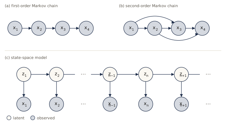
Two choices of the latent variables give the two main models of the chapter. If the \(\mathbf{z}_n\) are discrete, we get the hidden Markov model; its observations can be discrete or continuous. If the latent and observed variables are all Gaussian, with means that depend linearly on their parents, we get the linear dynamical system.
Hidden Markov models
The model
In a hidden Markov model (HMM) each latent variable \(\mathbf{z}_n\) takes one of \(K\) states. As in module 09 we write it in 1-of-\(K\) coding: \(\mathbf{z}_n\) is a binary vector with a single \(z_{nk} = 1\). Three ingredients define the model.
- The initial distribution \(\boldsymbol{\pi}\), with \(\pi_k = p(z_{1k} = 1)\) and \(\sum_k \pi_k = 1\), so \(p(\mathbf{z}_1 \mid \boldsymbol{\pi}) = \prod_k \pi_k^{z_{1k}}\).
- The transition matrix \(\mathbf{A}\), with \(A_{jk} = p(z_{nk} = 1 \mid z_{n-1,j} = 1)\). Each row is a distribution, so \(\sum_k A_{jk} = 1\) and \(\mathbf{A}\) has \(K(K-1)\) free parameters. In 1-of-\(K\) notation, \(p(\mathbf{z}_n \mid \mathbf{z}_{n-1}, \mathbf{A}) = \prod_{j} \prod_{k} A_{jk}^{z_{n-1,j} z_{nk}}\).
- The emission densities \(p(\mathbf{x}_n \mid \boldsymbol{\phi}_k)\), one per state, with parameters \(\boldsymbol{\phi} = \{\boldsymbol{\phi}_1, \dots, \boldsymbol{\phi}_K\}\), so that \(p(\mathbf{x}_n \mid \mathbf{z}_n, \boldsymbol{\phi}) = \prod_k p(\mathbf{x}_n \mid \boldsymbol{\phi}_k)^{z_{nk}}\). They can be Gaussians, tables for discrete symbols, mixtures, or anything else whose value we can evaluate.
With \(\mathbf{X} = \{\mathbf{x}_1, \dots, \mathbf{x}_N\}\), \(\mathbf{Z} = \{\mathbf{z}_1, \dots, \mathbf{z}_N\}\), and \(\boldsymbol{\theta} = \{\boldsymbol{\pi}, \mathbf{A}, \boldsymbol{\phi}\}\), the joint distribution is
\[p(\mathbf{X}, \mathbf{Z} \mid \boldsymbol{\theta}) = p(\mathbf{z}_1 \mid \boldsymbol{\pi}) \left[ \prod_{n=2}^{N} p(\mathbf{z}_n \mid \mathbf{z}_{n-1}, \mathbf{A}) \right] \prod_{n=1}^{N} p(\mathbf{x}_n \mid \mathbf{z}_n, \boldsymbol{\phi}).\]Look at a single time step and you see a mixture model: \(\mathbf{x}_n\) is drawn from one of \(K\) components. The difference from module 09 is that the component labels are no longer chosen independently at each step; each label depends on the previous one. If every row of \(\mathbf{A}\) were the same, the label would ignore its predecessor and we would be back to an ordinary mixture for i.i.d. data.
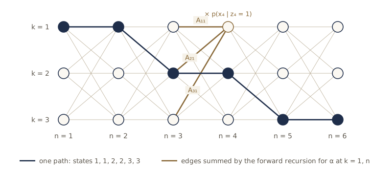
A state transition diagram, with one box per state and an arrow for each nonzero \(A_{jk}\), is a common way to draw \(\mathbf{A}\). It is not a graphical model: its nodes are values of a single variable, not separate random variables. Unrolling the diagram over time gives the trellis (or lattice) below, which we will use to picture the algorithms.
Generating data from an HMM is ancestral sampling along the graph: draw \(\mathbf{z}_1\) from \(\boldsymbol{\pi}\) and \(\mathbf{x}_1\) from its emission density, then \(\mathbf{z}_2\) from the row of \(\mathbf{A}\) selected by \(\mathbf{z}_1\), then \(\mathbf{x}_2\), and so on. Here is the HMM we use for the rest of the section: three states with one-dimensional Gaussian emissions, well separated means, and a strong tendency to stay put.
K = 3
pi_true = np.array([0.6, 0.3, 0.1])
A_true = np.array([[0.92, 0.06, 0.02],
                   [0.05, 0.90, 0.05],
                   [0.03, 0.07, 0.90]])
mu_true = np.array([-2.0, 0.0, 2.5])       # emission p(x | z = k) = N(x | mu_k, sigma_k^2)
sigma_true = np.array([0.7, 0.5, 1.0])

def sample_hmm(pi, A, mu, sigma, N, rng):
    """Ancestral sampling: z_1 ~ pi, z_n ~ row z_{n-1} of A,
    x_n ~ N(mu[z_n], sigma[z_n]^2)."""
    z = sample_chain(pi, A, N, rng)
    x = rng.normal(mu[z], sigma[z])
    return z, x

def gauss_logpdf(x, mu, sigma):
    """(N, K) array of ln N(x_n | mu_k, sigma_k^2): the log emission probabilities."""
    d = (np.asarray(x)[:, None] - mu) / sigma
    return -0.5 * d**2 - np.log(sigma) - 0.5 * np.log(2 * np.pi)

z_demo, x_demo = sample_hmm(pi_true, A_true, mu_true, sigma_true, 200,
                            np.random.default_rng(1))
print("states 1-60:", "".join(str(k + 1) for k in z_demo[:60]))
print("x_1..x_6:   ", np.round(x_demo[:6], 2))
states 1-60: 122222222111111111111113333333333333222222222222222222222222
x_1..x_6:    [-1.22  0.08  0.27 -0.53  0.91  1.01]
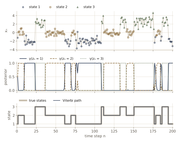
Because the diagonal of \(\mathbf{A}\) dominates, the states come in long runs, and so do the observations (the top panel of the decoding figure later in the module shows this sequence). Our task from here on is to go the other way: given only \(\mathbf{x}\), infer the states and learn the parameters.
Maximum likelihood and EM
To fit the model to an observed sequence we would like to maximize the likelihood
\[p(\mathbf{X} \mid \boldsymbol{\theta}) = \sum_{\mathbf{Z}} p(\mathbf{X}, \mathbf{Z} \mid \boldsymbol{\theta}).\]Two things make this hard. First, the joint does not factorize over \(n\) (neighboring \(\mathbf{z}\)’s are coupled), so we cannot sum out each \(\mathbf{z}_n\) separately as we did for mixtures; the sum is over all \(K^N\) paths through the trellis. Second, even if we could evaluate it, the logarithm of a sum has no closed-form maximizer, just as for a Gaussian mixture. The second problem has a familiar answer, the EM algorithm of module 09; the first will be solved by the forward–backward algorithm in the next subsection.
Recall how EM works. Starting from parameters \(\boldsymbol{\theta}^{\text{old}}\), the E step computes the posterior \(p(\mathbf{Z} \mid \mathbf{X}, \boldsymbol{\theta}^{\text{old}})\), and the M step picks new parameters that maximize the posterior expectation of the complete-data log likelihood
\[Q(\boldsymbol{\theta}, \boldsymbol{\theta}^{\text{old}}) = \sum_{\mathbf{Z}} p(\mathbf{Z} \mid \mathbf{X}, \boldsymbol{\theta}^{\text{old}}) \ln p(\mathbf{X}, \mathbf{Z} \mid \boldsymbol{\theta}).\]Take the logarithm of the joint. Every term is linear in a single \(z_{nk}\) or in a product \(z_{n-1,j} z_{nk}\) of two neighbors:
\[\ln p(\mathbf{X}, \mathbf{Z} \mid \boldsymbol{\theta}) = \sum_{k} z_{1k} \ln \pi_k + \sum_{n=2}^{N} \sum_{j,k} z_{n-1,j} z_{nk} \ln A_{jk} + \sum_{n=1}^{N} \sum_{k} z_{nk} \ln p(\mathbf{x}_n \mid \boldsymbol{\phi}_k).\]So the expectation needs only two kinds of posterior quantity, which get their own names:
\[\gamma(\mathbf{z}_n) = p(\mathbf{z}_n \mid \mathbf{X}, \boldsymbol{\theta}^{\text{old}}), \qquad \xi(\mathbf{z}_{n-1}, \mathbf{z}_n) = p(\mathbf{z}_{n-1}, \mathbf{z}_n \mid \mathbf{X}, \boldsymbol{\theta}^{\text{old}}).\]For each \(n\), \(\gamma(\mathbf{z}_n)\) is \(K\) numbers summing to one, and \(\xi(\mathbf{z}_{n-1}, \mathbf{z}_n)\) is a \(K \times K\) table summing to one. We write \(\gamma(z_{nk})\) for the probability that \(z_{nk} = 1\), which is also \(\mathbb{E}[z_{nk}]\) because \(z_{nk}\) is binary, and similarly \(\xi(z_{n-1,j}, z_{nk}) = \mathbb{E}[z_{n-1,j} z_{nk}]\). Taking the expectation of the log joint term by term,
\[Q(\boldsymbol{\theta}, \boldsymbol{\theta}^{\text{old}}) = \sum_{k} \gamma(z_{1k}) \ln \pi_k + \sum_{n=2}^{N} \sum_{j,k} \xi(z_{n-1,j}, z_{nk}) \ln A_{jk} + \sum_{n=1}^{N} \sum_{k} \gamma(z_{nk}) \ln p(\mathbf{x}_n \mid \boldsymbol{\phi}_k).\]M step for the transition matrix. Only the middle term involves \(\mathbf{A}\), and each row \(j\) appears in a separate group of terms, constrained to sum to one. Add a Lagrange multiplier \(\lambda_j\) for row \(j\) and set the derivative with respect to \(A_{jk}\) to zero:
\[\frac{\sum_{n=2}^{N} \xi(z_{n-1,j}, z_{nk})}{A_{jk}} + \lambda_j = 0 \quad\Longrightarrow\quad A_{jk} = \frac{\sum_{n=2}^{N} \xi(z_{n-1,j}, z_{nk})}{\sum_{l=1}^{K} \sum_{n=2}^{N} \xi(z_{n-1,j}, z_{nl})},\]where \(\lambda_j\) was fixed by the constraint. This is the counting formula for a Markov chain with the observed transition counts replaced by expected counts. The same argument for \(\boldsymbol{\pi}\) gives \(\pi_k = \gamma(z_{1k}) / \sum_j \gamma(z_{1j})\), which is just \(\gamma(z_{1k})\) since \(\gamma\) is normalized.
M step for the emissions. Only the last term involves \(\boldsymbol{\phi}\), and it has exactly the form of the corresponding term for a mixture model, with \(\gamma(z_{nk})\) playing the role of the responsibilities. If the \(\boldsymbol{\phi}_k\) are separate for each state, it splits into \(K\) weighted maximum likelihood problems. For Gaussian emissions \(\mathcal{N}(\mathbf{x} \mid \boldsymbol{\mu}_k, \boldsymbol{\Sigma}_k)\) the answer is the weighted mean and covariance, as in module 09:
\[\boldsymbol{\mu}_k = \frac{\sum_{n} \gamma(z_{nk}) \mathbf{x}_n}{\sum_{n} \gamma(z_{nk})}, \qquad \boldsymbol{\Sigma}_k = \frac{\sum_{n} \gamma(z_{nk}) (\mathbf{x}_n - \boldsymbol{\mu}_k)(\mathbf{x}_n - \boldsymbol{\mu}_k)^{\mathrm{T}}}{\sum_{n} \gamma(z_{nk})}.\]For discrete observations coded 1-of-\(D\), with emission table \(\mu_{ik} = p(x_i = 1 \mid z_k = 1)\), so that \(p(\mathbf{x} \mid \mathbf{z}) = \prod_{i} \prod_{k} \mu_{ik}^{x_i z_k}\), the update is the expected fraction of the time state \(k\) emits symbol \(i\): \(\mu_{ik} = \sum_n \gamma(z_{nk}) x_{ni} / \sum_n \gamma(z_{nk})\). Binary features with Bernoulli emissions work the same way.
Two practical points. EM needs starting values: \(\boldsymbol{\pi}\) and \(\mathbf{A}\) can start uniform or random (respecting the constraints), and Gaussian emissions can start from K-means clusters or from a mixture fit that ignores the time order. And any entry of \(\boldsymbol{\pi}\) or \(\mathbf{A}\) that starts at zero stays zero, because its expected count is always zero (exercise 2). That is a feature: it lets us impose structure, as in the left-to-right models below, simply by initializing some entries to zero.
With several independent training sequences \(\mathbf{X}^{(1)}, \dots, \mathbf{X}^{(R)}\), the log likelihood is a sum over sequences, and so is \(Q\). The E step runs separately on each sequence, and the M step adds up the expected counts and weighted sums across all of them before normalizing.
The forward–backward algorithm
The E step needs \(\gamma\) and \(\xi\) for every \(n\). We derive recursions for them from a few conditional independence properties of the HMM graph. All of them follow from d-separation (module 08), because the latent node between two parts of the chain blocks every path between them when it is given:
- Given \(\mathbf{z}_n\), the past observations \(\mathbf{x}_1, \dots, \mathbf{x}_n\) are independent of the future observations \(\mathbf{x}_{n+1}, \dots, \mathbf{x}_N\).
- Given \(\mathbf{z}_{n-1}\), the next latent variable \(\mathbf{z}_n\) is independent of \(\mathbf{x}_1, \dots, \mathbf{x}_{n-1}\).
- Given \(\mathbf{z}_n\), the observation \(\mathbf{x}_n\) is independent of all other latent variables and observations.
Throughout, the parameters are fixed at \(\boldsymbol{\theta}^{\text{old}}\), and we drop them from the notation. Define two sets of \(K\) numbers for each \(n\):
The forward variable is \(\alpha(\mathbf{z}_n) = p(\mathbf{x}_1, \dots, \mathbf{x}_n, \mathbf{z}_n)\), the joint probability of the observations so far and the current state. The backward variable is \(\beta(\mathbf{z}_n) = p(\mathbf{x}_{n+1}, \dots, \mathbf{x}_N \mid \mathbf{z}_n)\), the probability of the future observations given the current state.
Why they are what we need. By the product rule and property 1,
\[p(\mathbf{X}, \mathbf{z}_n) = p(\mathbf{x}_1, \dots, \mathbf{x}_n, \mathbf{z}_n) \, p(\mathbf{x}_{n+1}, \dots, \mathbf{x}_N \mid \mathbf{z}_n, \mathbf{x}_1, \dots, \mathbf{x}_n) = \alpha(\mathbf{z}_n) \beta(\mathbf{z}_n),\]so \(\gamma(\mathbf{z}_n) = \alpha(\mathbf{z}_n)\beta(\mathbf{z}_n) / p(\mathbf{X})\). Summing \(p(\mathbf{X}, \mathbf{z}_n)\) over \(\mathbf{z}_n\) gives the likelihood, \(p(\mathbf{X}) = \sum_{\mathbf{z}_n} \alpha(\mathbf{z}_n) \beta(\mathbf{z}_n)\), for any \(n\) we like.
Forward recursion. We want \(\alpha(\mathbf{z}_n)\) in terms of \(\alpha(\mathbf{z}_{n-1})\). Bring \(\mathbf{z}_{n-1}\) in and sum it out, then factor the joint with the product rule:
\[\begin{aligned} \alpha(\mathbf{z}_n) &= \sum_{\mathbf{z}_{n-1}} p(\mathbf{x}_1, \dots, \mathbf{x}_{n-1}, \mathbf{z}_{n-1}) \, p(\mathbf{z}_n \mid \mathbf{z}_{n-1}, \mathbf{x}_1, \dots, \mathbf{x}_{n-1}) \, p(\mathbf{x}_n \mid \mathbf{z}_n, \mathbf{z}_{n-1}, \mathbf{x}_1, \dots, \mathbf{x}_{n-1}) \\ &= p(\mathbf{x}_n \mid \mathbf{z}_n) \sum_{\mathbf{z}_{n-1}} \alpha(\mathbf{z}_{n-1}) \, p(\mathbf{z}_n \mid \mathbf{z}_{n-1}), \end{aligned}\]using property 2 for the middle factor and property 3 for the last. The recursion starts from \(\alpha(\mathbf{z}_1) = p(\mathbf{z}_1) p(\mathbf{x}_1 \mid \mathbf{z}_1)\), that is, \(\alpha(z_{1k}) = \pi_k \, p(\mathbf{x}_1 \mid \boldsymbol{\phi}_k)\). In words: to get to state \(k\) at step \(n\), collect the forward values of all states at step \(n-1\), weight them by the probability of moving to \(k\), and multiply by the probability that \(k\) emits \(\mathbf{x}_n\) (the brass edges in the trellis figure). Each step costs \(O(K^2)\), so the whole pass costs \(O(K^2 N)\) instead of the \(O(K^N)\) of enumerating paths. We have swapped the order of the sums and the products, so that at each step the contributions of all paths entering a state are added up once and for all.
Backward recursion. In the same way, bring \(\mathbf{z}_{n+1}\) in and sum it out:
\[\begin{aligned} \beta(\mathbf{z}_n) &= \sum_{\mathbf{z}_{n+1}} p(\mathbf{z}_{n+1} \mid \mathbf{z}_n) \, p(\mathbf{x}_{n+1} \mid \mathbf{z}_{n+1}) \, p(\mathbf{x}_{n+2}, \dots, \mathbf{x}_N \mid \mathbf{z}_{n+1}) \\ &= \sum_{\mathbf{z}_{n+1}} \beta(\mathbf{z}_{n+1}) \, p(\mathbf{x}_{n+1} \mid \mathbf{z}_{n+1}) \, p(\mathbf{z}_{n+1} \mid \mathbf{z}_n), \end{aligned}\]where, given \(\mathbf{z}_{n+1}\), the observations from \(n+1\) on no longer depend on \(\mathbf{z}_n\) and \(\mathbf{x}_{n+1}\) is independent of the later ones. To start it, set \(n = N\) in \(\gamma(\mathbf{z}_N) = \alpha(\mathbf{z}_N)\beta(\mathbf{z}_N)/p(\mathbf{X})\): since \(\alpha(\mathbf{z}_N) = p(\mathbf{X}, \mathbf{z}_N)\) already, we need \(\beta(\mathbf{z}_N) = 1\) for every state. As a by-product, \(p(\mathbf{X}) = \sum_{\mathbf{z}_N} \alpha(\mathbf{z}_N)\), so if we only want the likelihood, the forward pass alone is enough.
Pairwise posteriors. The same factorization with two neighboring states gives
\[\xi(\mathbf{z}_{n-1}, \mathbf{z}_n) = \frac{p(\mathbf{X}, \mathbf{z}_{n-1}, \mathbf{z}_n)}{p(\mathbf{X})} = \frac{\alpha(\mathbf{z}_{n-1}) \, p(\mathbf{z}_n \mid \mathbf{z}_{n-1}) \, p(\mathbf{x}_n \mid \mathbf{z}_n) \, \beta(\mathbf{z}_n)}{p(\mathbf{X})}:\]the observations up to \(n-1\) reach the pair through \(\alpha\), the transition and the emission of \(\mathbf{x}_n\) are explicit, and the rest of the future comes through \(\beta\).
In matrix form, with \(\boldsymbol{\alpha}_n\), \(\boldsymbol{\beta}_n\), and \(\mathbf{b}_n = (p(\mathbf{x}_n \mid \boldsymbol{\phi}_k))_k\) as length-\(K\) vectors and \(\odot\) the elementwise product, the recursions are \(\boldsymbol{\alpha}_n = \mathbf{b}_n \odot (\mathbf{A}^{\mathrm{T}} \boldsymbol{\alpha}_{n-1})\) and \(\boldsymbol{\beta}_n = \mathbf{A} (\mathbf{b}_{n+1} \odot \boldsymbol{\beta}_{n+1})\). Here is a direct implementation. It takes the emission probabilities as an \(N \times K\) array B, which is all the recursions need to know about the observations: nothing below depends on whether they are discrete or continuous, or on the form of the emission density.
def forward(pi, A, B):
    """alpha[n, k] = p(x_1..x_n, z_n = k), where B[n, k] = p(x_n | z_n = k). Unscaled."""
    N, K = B.shape
    alpha = np.empty((N, K))
    alpha[0] = pi * B[0]                             # alpha(z_1) = p(z_1) p(x_1 | z_1)
    for n in range(1, N):
        alpha[n] = B[n] * (alpha[n - 1] @ A)         # sum over z_{n-1}, then emit x_n
    return alpha

def backward(A, B):
    """beta[n, k] = p(x_{n+1}..x_N | z_n = k). Unscaled."""
    N, K = B.shape
    beta = np.ones((N, K))                            # beta(z_N) = 1
    for n in range(N - 2, -1, -1):
        beta[n] = A @ (B[n + 1] * beta[n + 1])
    return beta

def posteriors(pi, A, B):
    """p(X), gamma (N, K), and xi (N-1, K, K),
    where xi[n-1, j, k] = p(z_{n-1} = j, z_n = k | X)."""
    alpha, beta = forward(pi, A, B), backward(A, B)
    pX = alpha[-1].sum()
    gamma = alpha * beta / pX
    xi = alpha[:-1, :, None] * A[None] * (B[1:] * beta[1:])[:, None, :] / pX
    return pX, gamma, xi
For a short sequence we can afford to check this against the definition: list all \(K^N\) state paths, compute \(p(\mathbf{X}, \mathbf{Z})\) for each from the joint distribution, and add up. With \(N = 6\) there are 729 paths.
def path_log_joint(paths, log_pi, log_A, log_B):
    """ln p(X, Z) for every state path Z (one per row of `paths`, shape (P, N))."""
    lp = log_pi[paths[:, 0]] + log_B[0, paths[:, 0]]
    for n in range(1, paths.shape[1]):
        lp = lp + log_A[paths[:, n - 1], paths[:, n]] + log_B[n, paths[:, n]]
    return lp

x_short = x_demo[:6]
B_short = np.exp(gauss_logpdf(x_short, mu_true, sigma_true))
pX, gamma, xi = posteriors(pi_true, A_true, B_short)

paths = np.array(list(product(range(K), repeat=len(x_short))))       # all 3^6 paths
w = np.exp(path_log_joint(paths, np.log(pi_true), np.log(A_true), np.log(B_short)))
pX_bf = w.sum()
gamma_bf = np.array([[w[paths[:, n] == k].sum() for k in range(K)]
                     for n in range(6)]) / pX_bf
xi_bf = np.array([[[w[(paths[:, n - 1] == j) & (paths[:, n] == k)].sum() for k in range(K)]
                   for j in range(K)] for n in range(1, 6)]) / pX_bf

print(f"{len(paths)} paths.  p(X): forward = {pX:.6e}, brute force = {pX_bf:.6e}")
print(f"max error: gamma {np.abs(gamma - gamma_bf).max():.1e}, "
      f"xi {np.abs(xi - xi_bf).max():.1e}")
ab = forward(pi_true, A_true, B_short) * backward(A_true, B_short)
print("sum_k alpha*beta at each n:", ab.sum(axis=1))
print("gamma, first three steps:")
print(gamma[:3])
729 paths.  p(X): forward = 6.191095e-05, brute force = 6.191095e-05
max error: gamma 4.4e-16, xi 2.8e-16
sum_k alpha*beta at each n: [0.0001 0.0001 0.0001 0.0001 0.0001 0.0001]
gamma, first three steps:
[[0.5087 0.4912 0.0001]
 [0.0045 0.9951 0.0004]
 [0.     0.9997 0.0003]]
The forward–backward results agree with the brute-force sums to rounding error, and \(\sum_k \alpha(z_{nk})\beta(z_{nk})\) gives the same likelihood at every \(n\), as it should.
Prediction. The forward variables also give the predictive distribution of the next observation. Summing over the current and the next state,
\[p(\mathbf{x}_{N+1} \mid \mathbf{X}) = \sum_{\mathbf{z}_{N+1}} p(\mathbf{x}_{N+1} \mid \mathbf{z}_{N+1}) \sum_{\mathbf{z}_N} p(\mathbf{z}_{N+1} \mid \mathbf{z}_N) \frac{\alpha(\mathbf{z}_N)}{p(\mathbf{X})},\]a mixture of the emission densities with weights \(\mathbf{A}^{\mathrm{T}} \boldsymbol{\alpha}_N / p(\mathbf{X})\). The whole past is summarized by the \(K\) numbers in \(\boldsymbol{\alpha}_N\), so an online predictor needs only constant memory: when \(\mathbf{x}_{N+1}\) arrives, one more forward step updates the summary.
alpha_s = forward(pi_true, A_true, B_short)
w_next = (alpha_s[-1] / alpha_s[-1].sum()) @ A_true            # p(z_7 | x_1..x_6)
mean_next = w_next @ mu_true
var_next = w_next @ (sigma_true**2 + mu_true**2) - mean_next**2
print("p(z_7 | x_1..x_6):", w_next)
print(f"predictive mean of x_7: {mean_next:.4f}, std: {np.sqrt(var_next):.4f}")
p(z_7 | x_1..x_6): [0.0478 0.8085 0.1437]
predictive mean of x_7: 0.2637, std: 1.1787
After six observations the model puts most of its belief on state 2, so the predictive distribution of \(x_7\) is a mixture centered near state 2’s mean, with extra spread from the chance of a switch to state 1 or 3.
The sum-product view
The HMM graph is a tree, so module 08’s sum-product algorithm computes all the marginals exactly, and the forward–backward algorithm is what it becomes on this graph. Since we always condition on the observations, fold each emission into the neighboring transition and draw a chain-shaped factor graph over the latent variables alone, with factors
\[h(\mathbf{z}_1) = p(\mathbf{z}_1) \, p(\mathbf{x}_1 \mid \mathbf{z}_1), \qquad f_n(\mathbf{z}_{n-1}, \mathbf{z}_n) = p(\mathbf{z}_n \mid \mathbf{z}_{n-1}) \, p(\mathbf{x}_n \mid \mathbf{z}_n).\]Each variable node has only two neighbors, so it passes messages through unchanged, and the factor-to-variable messages obey
\[\mu_{f_n \to \mathbf{z}_n}(\mathbf{z}_n) = \sum_{\mathbf{z}_{n-1}} f_n(\mathbf{z}_{n-1}, \mathbf{z}_n) \, \mu_{f_{n-1} \to \mathbf{z}_{n-1}}(\mathbf{z}_{n-1}).\]This is the forward recursion, with \(\alpha(\mathbf{z}_n) = \mu_{f_n \to \mathbf{z}_n}(\mathbf{z}_n)\) and starting message \(h(\mathbf{z}_1)\). The messages from the end of the chain back toward the start are the \(\beta\)’s, starting from the constant message 1 at \(\mathbf{z}_N\). The sum-product rule for a marginal, the product of the incoming messages, gives \(p(\mathbf{z}_n, \mathbf{X}) = \alpha(\mathbf{z}_n)\beta(\mathbf{z}_n)\), and the rule for the variables of one factor gives \(\xi\). Bishop §13.2.3 writes this out; the point to keep is that nothing about the HMM needed a new idea beyond module 08.
Scaling factors
The recursions above are correct but not usable as written. Each forward step multiplies by transition and emission probabilities, which are typically well below 1, so \(\alpha(\mathbf{z}_n) \le p(\mathbf{x}_1, \dots, \mathbf{x}_n)\) shrinks roughly exponentially with \(n\). Watch it happen on a sequence of length 1000 from our HMM:
z_long, x_long = sample_hmm(pi_true, A_true, mu_true, sigma_true, 1000,
                            np.random.default_rng(2))
logB_long = gauss_logpdf(x_long, mu_true, sigma_true)
alpha_long = forward(pi_true, A_true, np.exp(logB_long))
p_prefix = alpha_long.sum(axis=1)                        # p(x_1..x_n)
for n in [10, 100, 300, 500, 1000]:
    print(f"n = {n:4d}:  p(x_1..x_n) = {p_prefix[n - 1]:.3e}")
print("first n with p(x_1..x_n) = 0:", np.argmax(p_prefix == 0) + 1)
n =   10:  p(x_1..x_n) = 2.669e-05
n =  100:  p(x_1..x_n) = 1.334e-55
n =  300:  p(x_1..x_n) = 1.051e-164
n =  500:  p(x_1..x_n) = 9.931e-279
n = 1000:  p(x_1..x_n) = 0.000e+00
first n with p(x_1..x_n) = 0: 595
Double precision cannot represent numbers much below \(10^{-308}\) (or, with reduced precision, \(10^{-323}\)), and from step 595 on every \(\alpha\) is exactly zero; \(\gamma = \alpha\beta/p(\mathbf{X})\) then becomes \(0/0\). For i.i.d. data we avoided this by working with log likelihoods, but here the recursion adds up products, so a plain logarithm does not pass through it. (We could carry \(\ln \alpha\) and use log-sum-exp for every sum; that works, and we use it below as a check, but it is slower.) The standard fix is to normalize at every step.
Define the scaled forward variable as the posterior of \(\mathbf{z}_n\) given the data so far, and a scaling factor \(c_n\) as the predictive probability of each new observation:
\[\hat{\alpha}(\mathbf{z}_n) = p(\mathbf{z}_n \mid \mathbf{x}_1, \dots, \mathbf{x}_n) = \frac{\alpha(\mathbf{z}_n)}{p(\mathbf{x}_1, \dots, \mathbf{x}_n)}, \qquad c_n = p(\mathbf{x}_n \mid \mathbf{x}_1, \dots, \mathbf{x}_{n-1}).\]The \(\hat{\alpha}\)’s are distributions over \(K\) states, so they stay of order one. By the product rule \(p(\mathbf{x}_1, \dots, \mathbf{x}_n) = \prod_{m=1}^{n} c_m\), and hence \(\alpha(\mathbf{z}_n) = \left( \prod_{m \le n} c_m \right) \hat{\alpha}(\mathbf{z}_n)\). Substituting this into the forward recursion and cancelling \(\prod_{m \le n-1} c_m\) from both sides gives
\[c_n \, \hat{\alpha}(\mathbf{z}_n) = p(\mathbf{x}_n \mid \mathbf{z}_n) \sum_{\mathbf{z}_{n-1}} \hat{\alpha}(\mathbf{z}_{n-1}) \, p(\mathbf{z}_n \mid \mathbf{z}_{n-1}).\]We never need to compute \(c_n\) separately: it is the number that normalizes the right-hand side, and \(\hat{\alpha}(\mathbf{z}_n)\) is what is left after dividing by it. For the backward pass define \(\hat{\beta}(\mathbf{z}_n) = \beta(\mathbf{z}_n) / \prod_{m=n+1}^{N} c_m\), which is the ratio \(p(\mathbf{x}_{n+1}, \dots, \mathbf{x}_N \mid \mathbf{z}_n) / p(\mathbf{x}_{n+1}, \dots, \mathbf{x}_N \mid \mathbf{x}_1, \dots, \mathbf{x}_n)\) and so also stays moderate. The same substitution turns the backward recursion into
\[c_{n+1} \, \hat{\beta}(\mathbf{z}_n) = \sum_{\mathbf{z}_{n+1}} \hat{\beta}(\mathbf{z}_{n+1}) \, p(\mathbf{x}_{n+1} \mid \mathbf{z}_{n+1}) \, p(\mathbf{z}_{n+1} \mid \mathbf{z}_n),\]reusing the \(c_n\) stored in the forward pass. Everything we need follows, with the products of \(c\)’s cancelling:
Result. With scaled variables, \(\ln p(\mathbf{X}) = \sum_{n=1}^{N} \ln c_n\), \(\gamma(\mathbf{z}_n) = \hat{\alpha}(\mathbf{z}_n) \hat{\beta}(\mathbf{z}_n)\), and \(\xi(\mathbf{z}_{n-1}, \mathbf{z}_n) = c_n^{-1} \, \hat{\alpha}(\mathbf{z}_{n-1}) \, p(\mathbf{x}_n \mid \mathbf{z}_n) \, p(\mathbf{z}_n \mid \mathbf{z}_{n-1}) \, \hat{\beta}(\mathbf{z}_n)\).
For \(\xi\), the \(\alpha\) contributes \(\prod_{m \le n-1} c_m\) and the \(\beta\) contributes \(\prod_{m > n} c_m\); divided by \(p(\mathbf{X}) = \prod_m c_m\), only \(c_n^{-1}\) is left.
One more safeguard is cheap. A far outlier can make \(p(\mathbf{x}_n \mid \boldsymbol{\phi}_k)\) itself underflow for every \(k\). Since we are given log emission probabilities, we subtract the largest one at each \(n\) before exponentiating; this multiplies row \(n\) of \(\mathbf{B}\) by a constant, which rescales \(c_n\) and nothing else, and we add the constant back to the log likelihood.
def forward_backward(pi, A, logB):
    """Scaled forward-backward. logB[n, k] = ln p(x_n | z_n = k).
    Returns gamma (N, K), xi (N-1, K, K), and ln p(X)."""
    shift = logB.max(axis=1, keepdims=True)
    B = np.exp(logB - shift)                      # rows rescaled; undone in ln p(X) below
    N, K = B.shape
    alpha_hat, c = np.empty((N, K)), np.empty(N)
    a = pi * B[0]
    c[0] = a.sum(); alpha_hat[0] = a / c[0]
    for n in range(1, N):
        a = B[n] * (alpha_hat[n - 1] @ A)             # c_n * alpha_hat(z_n)
        c[n] = a.sum(); alpha_hat[n] = a / c[n]
    beta_hat = np.ones((N, K))
    for n in range(N - 2, -1, -1):
        beta_hat[n] = A @ (B[n + 1] * beta_hat[n + 1]) / c[n + 1]
    gamma = alpha_hat * beta_hat
    xi = (alpha_hat[:-1, :, None] * A[None] * (B[1:] * beta_hat[1:])[:, None, :]
          / c[1:, None, None])
    loglik = np.log(c).sum() + shift.sum()            # ln p(X) = sum_n ln c_n
    return gamma, xi, loglik

def log_forward(log_pi, log_A, logB):
    """ln p(X) by carrying ln alpha with log-sum-exp: a slower, independent check."""
    la = log_pi + logB[0]
    for n in range(1, len(logB)):
        la = logB[n] + logsumexp(la[:, None] + log_A, axis=0)
    return logsumexp(la)

logB_short = gauss_logpdf(x_short, mu_true, sigma_true)
g_s, xi_s, ll_s = forward_backward(pi_true, A_true, logB_short)
print(f"N = 6:    ln p(X) scaled = {ll_s:.6f}, unscaled = {np.log(pX):.6f}")
print(f"          max difference: gamma {np.abs(g_s - gamma).max():.1e}, "
      f"xi {np.abs(xi_s - xi).max():.1e}")
g_long, xi_long, ll_long = forward_backward(pi_true, A_true, logB_long)
ll_check = log_forward(np.log(pi_true), np.log(A_true), logB_long)
print(f"N = 1000: ln p(X) scaled = {ll_long:.4f}, log-space = {ll_check:.4f}")
print("          gamma rows sum to 1:", np.allclose(g_long.sum(axis=1), 1),
      "  xi summed over k equals gamma:", np.allclose(xi_long.sum(axis=2), g_long[:-1]))
N = 6:    ln p(X) scaled = -9.689813, unscaled = -9.689813
          max difference: gamma 4.4e-16, xi 3.3e-16
N = 1000: ln p(X) scaled = -1260.7502, log-space = -1260.7502
          gamma rows sum to 1: True   xi summed over k equals gamma: True
The scaled pass matches the unscaled one on the short sequence and the log-space pass on the long one, where the unscaled version gave zeros.
There is a second common form of the backward pass that recurses directly on \(\gamma(\mathbf{z}_n) = \hat{\alpha}(\mathbf{z}_n)\hat{\beta}(\mathbf{z}_n)\) instead of on \(\hat{\beta}\). It needs the forward pass to finish first, whereas the \(\alpha\) and \(\beta\) passes can run independently. For HMMs the \(\alpha\)–\(\beta\) form is the usual one; for linear dynamical systems the \(\alpha\)–\(\gamma\) form is, and we will meet it as the RTS smoother.
Baum–Welch: EM for the HMM
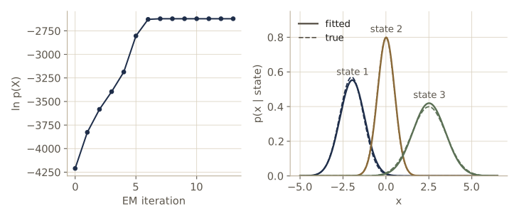
We now have everything for EM, which for HMMs is known as the Baum–Welch algorithm: run the scaled forward–backward pass on each training sequence to get \(\gamma\) and \(\xi\) (E step), then apply the updates for \(\boldsymbol{\pi}\), \(\mathbf{A}\), and the emission parameters (M step), and repeat. The log likelihood \(\sum_n \ln c_n\) comes for free from the E step, so we can monitor it; EM guarantees that it never decreases.
def baum_welch(xs, pi, A, mu, sigma, max_iter=200, tol=1e-6):
    """EM for an HMM with 1-D Gaussian emissions, on a list of sequences xs.
    Returns the fitted parameters and ln p(X | theta) at the start of each iteration."""
    K = len(pi)
    history = []
    for it in range(max_iter):
        g1, xi_sum = np.zeros(K), np.zeros((K, K))
        s0, s1, s2 = np.zeros(K), np.zeros(K), np.zeros(K)
        loglik = 0.0
        for x in xs:                                            # E step, sequence by sequence
            gamma, xi, ll = forward_backward(pi, A, gauss_logpdf(x, mu, sigma))
            g1 += gamma[0]                                      # expected initial states
            xi_sum += xi.sum(axis=0)                            # expected transition counts
            s0 += gamma.sum(axis=0); s1 += gamma.T @ x; s2 += gamma.T @ x**2
            loglik += ll
        history.append(loglik)
        pi = g1 / g1.sum()                                      # M step
        A = xi_sum / xi_sum.sum(axis=1, keepdims=True)
        mu = s1 / s0                                            # weighted means
        sigma = np.sqrt(s2 / s0 - mu**2)                        # weighted standard deviations
        if it > 0 and history[-1] - history[-2] < tol:
            break
    return pi, A, mu, sigma, np.array(history)
We train on five sequences of length 400 from the true model. For initialization we take uniform \(\boldsymbol{\pi}\) and \(\mathbf{A}\), put the three means at the 1/6, 1/2, and 5/6 quantiles of the pooled data, and give every state the pooled standard deviation. Uniform rows of \(\mathbf{A}\) mean the first E step treats the data as an ordinary mixture; the time structure is learned from there.
data_rng = np.random.default_rng(3)
train = [sample_hmm(pi_true, A_true, mu_true, sigma_true, 400, data_rng) for _ in range(5)]
xs = [x for _, x in train]
pooled = np.concatenate(xs)

pi0, A0 = np.full(K, 1 / K), np.full((K, K), 1 / K)
mu0, sigma0 = np.quantile(pooled, [1/6, 1/2, 5/6]), np.full(K, pooled.std())
pi_est, A_est, mu_est, sigma_est, hist = baum_welch(xs, pi0, A0, mu0, sigma0)

for it in [0, 1, 2, 5, 8, len(hist) - 1]:
    print(f"iteration {it:2d}: ln p(X) = {hist[it]:10.4f}")
assert np.all(np.diff(hist) > -1e-8), "EM decreased the likelihood"
print(f"{len(hist)} iterations; the log likelihood never decreased "
      f"(smallest change {np.diff(hist).min():.1e})")
iteration  0: ln p(X) = -4210.1518
iteration  1: ln p(X) = -3827.0740
iteration  2: ln p(X) = -3583.2843
iteration  5: ln p(X) = -2804.1995
iteration  8: ln p(X) = -2621.8338
iteration 13: ln p(X) = -2621.8289
14 iterations; the log likelihood never decreased (smallest change 3.2e-07)
A hidden state has no name, so EM can only recover the states up to a relabeling: any permutation of the labels, applied consistently to \(\boldsymbol{\pi}\), the rows and columns of \(\mathbf{A}\), and the emission parameters, gives exactly the same likelihood. To compare with the truth we sort the fitted states by their means, the order the true states happen to be in.
order = np.argsort(mu_est)                     # relabel the fitted states by increasing mean
print("pi     true", pi_true, "  fitted", pi_est[order])
print("mu     true", mu_true, "  fitted", mu_est[order])
print("sigma  true", sigma_true, "  fitted", sigma_est[order])
print("A true:")
print(A_true)
print("A fitted:")
print(A_est[np.ix_(order, order)])
ll_true = sum(forward_backward(pi_true, A_true, gauss_logpdf(x, mu_true, sigma_true))[2]
              for x in xs)
print(f"ln p(X): fitted {hist[-1]:.2f}, true parameters {ll_true:.2f}")
pi     true [0.6 0.3 0.1]   fitted [0.3941 0.6059 0.    ]
mu     true [-2.   0.   2.5]   fitted [-1.9588  0.0133  2.5114]
sigma  true [0.7 0.5 1. ]   fitted [0.7218 0.4991 0.9508]
A true:
[[0.92 0.06 0.02]
 [0.05 0.9  0.05]
 [0.03 0.07 0.9 ]]
A fitted:
[[0.9399 0.0466 0.0135]
 [0.0461 0.9067 0.0472]
 [0.0157 0.0829 0.9013]]
ln p(X): fitted -2621.83, true parameters -2629.99
The emission parameters and the transition matrix are recovered to within a few hundredths from 2000 observations, and the fitted model has a slightly higher likelihood on the training data than the true parameters, as a maximum likelihood fit should. The initial distribution is the exception. Only the first state of each sequence informs \(\boldsymbol{\pi}\), so here it is estimated from five data points, and a state that never starts a sequence gets \(\pi_k = 0\). With few sequences, \(\boldsymbol{\pi}\) is better fixed or given a prior.
Watch out. Like EM for mixtures, Baum–Welch finds a local maximum, and the result depends on the initialization. Two states can end up sharing one true regime while another regime is split, and with Gaussian emissions a state that captures a single point can drive its variance to zero and the likelihood to infinity. In practice: initialize sensibly (K-means or a mixture fit), run from several starts and keep the best likelihood, and put a floor or a prior on the variances.
The maximum likelihood framework extends in the usual ways. Adding a log prior on \(\boldsymbol{\theta}\) to \(Q\) gives MAP estimation with the same E step; for instance, a Dirichlet prior on each row of \(\mathbf{A}\) adds pseudo-counts to the expected transition counts. A fully Bayesian treatment that averages over the parameters can be done with the variational methods of module 10, and again leads to forward and backward passes.
The Viterbi algorithm
Often the states mean something, such as the phoneme being spoken, the gene region a base belongs to, or the regime a market is in, and we want the single most probable explanation of the data: the state sequence
\[\mathbf{Z}^{\star} = \arg\max_{\mathbf{Z}} p(\mathbf{X}, \mathbf{Z}) = \arg\max_{\mathbf{Z}} p(\mathbf{Z} \mid \mathbf{X}).\]This is not the same as taking the most probable state at each step from \(\gamma\). The per-step choices maximize the expected number of correct states, but pieced together they need not form a probable sequence; if \(\mathbf{A}\) has zeros, they can even form an impossible one (exercise 4). The whole-sequence maximization is the max-sum algorithm of module 08 applied to the HMM chain, and it is called the Viterbi algorithm.
It is easiest to derive directly. Define, for each state at step \(n\), the log probability of the best path that ends there:
\[\omega(\mathbf{z}_n) = \max_{\mathbf{z}_1, \dots, \mathbf{z}_{n-1}} \ln p(\mathbf{x}_1, \dots, \mathbf{x}_n, \mathbf{z}_1, \dots, \mathbf{z}_n).\]The log joint of a path up to step \(n\) is the log joint up to step \(n-1\) plus \(\ln p(\mathbf{z}_n \mid \mathbf{z}_{n-1}) + \ln p(\mathbf{x}_n \mid \mathbf{z}_n)\), and only the first of these depends on \(\mathbf{z}_1, \dots, \mathbf{z}_{n-2}\). So we can maximize over the early states first, and
\[\omega(\mathbf{z}_n) = \ln p(\mathbf{x}_n \mid \mathbf{z}_n) + \max_{\mathbf{z}_{n-1}} \left\{ \ln p(\mathbf{z}_n \mid \mathbf{z}_{n-1}) + \omega(\mathbf{z}_{n-1}) \right\}, \qquad \omega(\mathbf{z}_1) = \ln p(\mathbf{z}_1) + \ln p(\mathbf{x}_1 \mid \mathbf{z}_1).\]This is the forward recursion with the sum replaced by a max, done in logs. Logs make scaling unnecessary: sums of logs of probabilities do not underflow. The best final value, \(\max_{\mathbf{z}_N} \omega(\mathbf{z}_N)\), is \(\ln p(\mathbf{X}, \mathbf{Z}^{\star})\). To recover the path itself, record for each state \(k\) at step \(n\) which predecessor achieved the max, \(\psi_n(k)\). After the last step, start from the best final state and follow the pointers back: \(k_{n-1}^{\star} = \psi_n(k_n^{\star})\).
The intuition: many paths enter each node of the trellis, but only the best of them can be part of the overall best path through that node, so we keep one survivor per state, \(K\) in all. Each step considers \(K^2\) extensions and keeps \(K\), for a total cost of \(O(K^2 N)\).
def viterbi(log_pi, log_A, log_B):
    """Most probable state path and its log joint probability ln p(X, Z*)."""
    N, K = log_B.shape
    omega = np.empty((N, K))
    psi = np.zeros((N, K), dtype=int)
    omega[0] = log_pi + log_B[0]
    for n in range(1, N):
        scores = omega[n - 1][:, None] + log_A      # scores[j, k]: best path to j, then j -> k
        psi[n] = scores.argmax(axis=0)              # best predecessor of each state k
        omega[n] = log_B[n] + scores.max(axis=0)
    path = np.empty(N, dtype=int)
    path[-1] = omega[-1].argmax()
    for n in range(N - 1, 0, -1):                   # backtrack
        path[n - 1] = psi[n, path[n]]
    return path, omega[-1].max()

log_pi_t, log_A_t = np.log(pi_true), np.log(A_true)
x8 = x_demo[18:26]                                  # a stretch with a change of state
logB8 = gauss_logpdf(x8, mu_true, sigma_true)
path_v, lp_v = viterbi(log_pi_t, log_A_t, logB8)
paths8 = np.array(list(product(range(K), repeat=8)))                  # 3^8 = 6561 paths
lp_all = path_log_joint(paths8, log_pi_t, log_A_t, logB8)
print("Viterbi path:    ", path_v + 1, f" ln p(X, Z*) = {lp_v:.6f}")
print("brute-force best:", paths8[lp_all.argmax()] + 1, f" ln p(X, Z*) = {lp_all.max():.6f}")
Viterbi path:     [1 1 1 1 1 3 3 3]  ln p(X, Z*) = -11.730451
brute-force best: [1 1 1 1 1 3 3 3]  ln p(X, Z*) = -11.730451
The recursion finds the same path as the exhaustive search over all 6561 paths: five steps in state 1, then a switch to state 3, which is also what generated this stretch.
On the length-1000 sequence we can compare the Viterbi path with the per-step choices from \(\gamma\), and both with the true states:
path_v, lp_v = viterbi(log_pi_t, log_A_t, logB_long)
path_g = g_long.argmax(axis=1)                          # most probable state at each step
lp_g = path_log_joint(path_g[None], log_pi_t, log_A_t, logB_long)[0]
print(f"agreement with the true states: Viterbi {np.mean(path_v == z_long):.3f}, "
      f"per-step argmax {np.mean(path_g == z_long):.3f}")
print(f"steps where the two decodings differ: {np.sum(path_v != path_g)}")
print(f"ln p(X, Z): Viterbi {lp_v:.2f}, per-step argmax {lp_g:.2f}, true states "
      f"{path_log_joint(z_long[None], log_pi_t, log_A_t, logB_long)[0]:.2f}")
agreement with the true states: Viterbi 0.994, per-step argmax 0.994
steps where the two decodings differ: 0
ln p(X, Z): Viterbi -1270.86, per-step argmax -1270.86, true states -1285.65
Both decodings recover the true state at more than 99% of the steps, and on this sequence they agree everywhere: our states are well separated and persistent, so the posterior is nearly certain almost everywhere, and the two criteria pick the same path. They part ways when the evidence is ambiguous for several steps in a row, and exercise 4 builds a case where the per-step choices form an impossible path. Note also that the true state sequence has a lower joint probability than the Viterbi path: the most probable explanation is not the truth, only the best guess given the data.
Extensions of the hidden Markov model
The basic HMM has been extended in many directions. Here are the most important, briefly; Bishop §13.2.6 and the Rabiner tutorial in “Going further” have more.
Left-to-right models. Setting \(A_{jk} = 0\) for \(k < j\) gives a left-to-right HMM: once the chain leaves a state it can never return, and every sequence usually starts in state 1 (\(\pi_1 = 1\)). Often the jumps are also limited, \(A_{jk} = 0\) for \(k > j + \Delta\). Such models suit signals that pass through a fixed series of phases, such as a spoken word or a handwritten stroke. Because the chain can linger in each state for a variable number of steps, the model tolerates stretching and compressing of the time axis, which is what makes HMMs robust to variations in speaking rate. EM needs no change: zeros in the initial \(\mathbf{A}\) stay zero. Since each forward transition is seen at most once per sequence, left-to-right models must be trained on many sequences.
Discriminative training. When HMMs are used to classify sequences, with one model \(\boldsymbol{\theta}_m\) per class, maximum likelihood fits each class model to its own data without regard to the others. An alternative trains all class models together to maximize \(\sum_r \ln p(m_r \mid \mathbf{X}_r)\), the log probability of the correct labels, which by Bayes’ theorem is a function of the sequence likelihoods \(p(\mathbf{X}_r \mid \boldsymbol{\theta}_m)\) and the class priors. This is the cross-entropy criterion of module 04; it is harder to optimize, because every training sequence must be scored under every model.
State durations. An HMM that enters state \(k\) stays there for exactly \(T \ge 1\) steps with probability \(p(T) = A_{kk}^{T-1}(1 - A_{kk})\): a geometric distribution, whose most likely value is always \(T = 1\). Many real processes have durations that cluster around a typical value instead. A check on a long simulated run of our HMM, printing each empirical value next to the geometric prediction:
z_run = sample_chain(pi_true, A_true, 50000, np.random.default_rng(4))
starts = np.r_[0, np.flatnonzero(np.diff(z_run)) + 1]
lengths = np.diff(np.r_[starts, len(z_run)])[:-1]            # drop the last (unfinished) run
states = z_run[starts][:-1]
for k in range(K):
    T_k = lengths[states == k]
    a = A_true[k, k]
    print(f"state {k + 1}: mean {T_k.mean():5.2f} vs {1 / (1 - a):5.2f};  "
          f"P(T=1) {np.mean(T_k == 1):.3f} vs {1 - a:.3f};  "
          f"P(T=10) {np.mean(T_k == 10):.3f} vs {a**9 * (1 - a):.3f}")
state 1: mean 12.67 vs 12.50;  P(T=1) 0.089 vs 0.080;  P(T=10) 0.043 vs 0.038
state 2: mean  9.82 vs 10.00;  P(T=1) 0.111 vs 0.100;  P(T=10) 0.036 vs 0.039
state 3: mean  9.64 vs 10.00;  P(T=1) 0.099 vs 0.100;  P(T=10) 0.042 vs 0.039
The simulated run lengths follow the geometric law closely: the mean duration is about \(1/(1 - A_{kk})\), and for every state a run of a single step is more common than a run of ten, however sticky the state. A semi-Markov or explicit-duration model fixes this by giving each state its own duration distribution \(p(T \mid k)\), setting \(A_{kk} = 0\), and emitting \(T\) observations each time a state is entered. EM still works, with modified recursions.
Autoregressive HMMs. Correlations between observations far apart in time must pass through the latent chain, which an HMM does poorly. An autoregressive HMM adds arrows from a few previous observations to \(\mathbf{x}_n\), so that, for Gaussian emissions, the mean of \(\mathbf{x}_n\) is a linear function of \(\mathbf{x}_{n-1}, \mathbf{x}_{n-2}, \dots\) with coefficients that depend on the state: an AR model per regime. The latent chain keeps its Markov property (conditioning on \(\mathbf{z}_n\) still separates the past states from the future ones, since the extra paths pass head-to-tail through observed nodes), so forward–backward still works, and the M step for the emissions becomes weighted linear regression.
Input–output HMMs. In an input–output HMM a second observed sequence \(\mathbf{u}_1, \dots, \mathbf{u}_N\) of inputs influences the transitions, the emissions, or both, and we maximize the conditional likelihood \(p(\mathbf{X} \mid \mathbf{U}, \boldsymbol{\theta})\). This brings HMMs to supervised learning of sequence-to-sequence maps. Again the latent chain stays Markov, and EM with forward–backward applies.
Factorial HMMs. A factorial HMM has \(M\) independent latent chains that jointly produce each observation. Ten binary chains can represent \(2^{10} = 1024\) joint configurations with far fewer parameters than a 1024-state HMM. The difficulty is inference: once \(\mathbf{x}_n\) is observed, its parents in different chains become dependent (it is a head-to-head node), so the chains cannot be processed separately. Merging them into one chain with \(K^M\) states is exact but costs \(O(N K^{2M})\); the practical alternatives are the sampling methods of module 11 and variational approximations (module 10) that run forward–backward on each chain separately.
Linear dynamical systems
The model
Suppose a sensor measures a quantity \(z\) with zero-mean Gaussian noise. If \(z\) is constant, the best estimate from many measurements is their average. If \(z\) changes over time, a plain average blurs the changes, so we might average only the last few measurements, or weight recent ones more heavily. How many, and with what weights? The answer should depend on how fast \(z\) moves compared to how noisy the sensor is. A probabilistic model of both processes answers the question for us.
A linear dynamical system (LDS) is the state-space model with continuous latent variables and linear-Gaussian conditionals:
\[p(\mathbf{z}_n \mid \mathbf{z}_{n-1}) = \mathcal{N}(\mathbf{z}_n \mid \mathbf{A} \mathbf{z}_{n-1}, \boldsymbol{\Gamma}), \qquad p(\mathbf{x}_n \mid \mathbf{z}_n) = \mathcal{N}(\mathbf{x}_n \mid \mathbf{C} \mathbf{z}_n, \boldsymbol{\Sigma}), \qquad p(\mathbf{z}_1) = \mathcal{N}(\mathbf{z}_1 \mid \boldsymbol{\mu}_0, \mathbf{V}_0).\]Equivalently, as noisy linear equations,
\[\mathbf{z}_n = \mathbf{A} \mathbf{z}_{n-1} + \mathbf{w}_n, \qquad \mathbf{x}_n = \mathbf{C} \mathbf{z}_n + \mathbf{v}_n, \qquad \mathbf{z}_1 = \boldsymbol{\mu}_0 + \mathbf{u},\]with independent noise \(\mathbf{w}_n \sim \mathcal{N}(\mathbf{0}, \boldsymbol{\Gamma})\), \(\mathbf{v}_n \sim \mathcal{N}(\mathbf{0}, \boldsymbol{\Sigma})\), and \(\mathbf{u} \sim \mathcal{N}(\mathbf{0}, \mathbf{V}_0)\). The parameters are \(\boldsymbol{\theta} = \{\mathbf{A}, \boldsymbol{\Gamma}, \mathbf{C}, \boldsymbol{\Sigma}, \boldsymbol{\mu}_0, \mathbf{V}_0\}\). The matrix \(\mathbf{A}\) now describes the dynamics of a continuous state, not transition probabilities, and \(\mathbf{C}\) says how the state is observed. (Constant offsets in the means are easy to add; we leave them out.)
Each pair \((\mathbf{z}_n, \mathbf{x}_n)\) on its own is a linear-Gaussian latent variable model like probabilistic PCA or factor analysis (module 12); the LDS lets the latent variables drift in time. Just as the HMM extends mixture models to sequences, the LDS extends continuous latent variable models.
Why Gaussians? For inference along the chain to stay cheap, the message passed from one step to the next must keep its form, changing only its parameters. With linear-Gaussian conditionals it does: the joint distribution of all the \(\mathbf{z}\)’s and \(\mathbf{x}\)’s is one big Gaussian, and so is every marginal and conditional we will need. If instead the emission were a mixture of \(K\) Gaussians, the posterior over \(\mathbf{z}_1\) would be a \(K\)-component mixture, over \(\mathbf{z}_2\) a \(K^2\)-component mixture, and so on, growing without bound.
A consequence of joint Gaussianity: the most probable latent sequence is simply the sequence of posterior means, because a Gaussian’s mode is its mean and the marginals of a Gaussian have the same means. So the LDS needs no separate Viterbi algorithm (exercise 9).
Inference: the Kalman filter
The inference problems are those of the HMM. Filtering asks for \(p(\mathbf{z}_n \mid \mathbf{x}_1, \dots, \mathbf{x}_n)\), the current state given the data so far, which is what a real-time tracker needs; smoothing asks for \(p(\mathbf{z}_n \mid \mathbf{x}_1, \dots, \mathbf{x}_N)\), using the future too, which is what learning needs. Because the graph is the same, the algorithms have the same shape as the scaled forward–backward recursions, with sums over \(\mathbf{z}_{n-1}\) replaced by integrals. The forward pass is the Kalman filter and the backward pass the Kalman smoother, or Rauch–Tung–Striebel (RTS) smoother.
We write the filtered distribution, the analog of \(\hat{\alpha}\), as
\[\hat{\alpha}(\mathbf{z}_n) = p(\mathbf{z}_n \mid \mathbf{x}_1, \dots, \mathbf{x}_n) = \mathcal{N}(\mathbf{z}_n \mid \boldsymbol{\mu}_n, \mathbf{V}_n),\]and the recursion to solve is the scaled forward recursion with an integral:
\[c_n \, \hat{\alpha}(\mathbf{z}_n) = p(\mathbf{x}_n \mid \mathbf{z}_n) \int \hat{\alpha}(\mathbf{z}_{n-1}) \, p(\mathbf{z}_n \mid \mathbf{z}_{n-1}) \, d\mathbf{z}_{n-1}.\]Everything we need is in the pair of Gaussian identities from module 02. If
\[p(\mathbf{u}) = \mathcal{N}(\mathbf{u} \mid \mathbf{m}, \mathbf{M}), \qquad p(\mathbf{y} \mid \mathbf{u}) = \mathcal{N}(\mathbf{y} \mid \mathbf{F}\mathbf{u}, \mathbf{R}),\]then (I) the marginal is \(p(\mathbf{y}) = \mathcal{N}(\mathbf{y} \mid \mathbf{F}\mathbf{m}, \mathbf{F}\mathbf{M}\mathbf{F}^{\mathrm{T}} + \mathbf{R})\), and (II) the posterior is \(p(\mathbf{u} \mid \mathbf{y}) = \mathcal{N}(\mathbf{u} \mid \mathbf{S}(\mathbf{F}^{\mathrm{T}}\mathbf{R}^{-1}\mathbf{y} + \mathbf{M}^{-1}\mathbf{m}), \mathbf{S})\) with \(\mathbf{S} = (\mathbf{M}^{-1} + \mathbf{F}^{\mathrm{T}}\mathbf{R}^{-1}\mathbf{F})^{-1}\).
Form (II) involves inverses of state-sized matrices. For filtering we want a form that inverts only an observation-sized matrix, and that exposes a useful quantity. Define the gain
\[\mathbf{G} = \mathbf{M}\mathbf{F}^{\mathrm{T}} (\mathbf{F}\mathbf{M}\mathbf{F}^{\mathrm{T}} + \mathbf{R})^{-1}.\]By the Woodbury identity (Bishop appendix C), \(\mathbf{S} = \mathbf{M} - \mathbf{M}\mathbf{F}^{\mathrm{T}}(\mathbf{F}\mathbf{M}\mathbf{F}^{\mathrm{T}} + \mathbf{R})^{-1}\mathbf{F}\mathbf{M} = (\mathbf{I} - \mathbf{G}\mathbf{F})\mathbf{M}\). By the “push-through” identity \((\mathbf{M}^{-1} + \mathbf{F}^{\mathrm{T}}\mathbf{R}^{-1}\mathbf{F})^{-1}\mathbf{F}^{\mathrm{T}}\mathbf{R}^{-1} = \mathbf{M}\mathbf{F}^{\mathrm{T}}(\mathbf{F}\mathbf{M}\mathbf{F}^{\mathrm{T}} + \mathbf{R})^{-1}\) (multiply both sides on the left by \(\mathbf{M}^{-1} + \mathbf{F}^{\mathrm{T}}\mathbf{R}^{-1}\mathbf{F}\) and on the right by \(\mathbf{F}\mathbf{M}\mathbf{F}^{\mathrm{T}} + \mathbf{R}\) to check it), \(\mathbf{S}\mathbf{F}^{\mathrm{T}}\mathbf{R}^{-1} = \mathbf{G}\). So the posterior mean is \(\mathbf{G}\mathbf{y} + (\mathbf{I} - \mathbf{G}\mathbf{F})\mathbf{m}\), and
\[p(\mathbf{u} \mid \mathbf{y}) = \mathcal{N}\big(\mathbf{u} \mid \mathbf{m} + \mathbf{G}(\mathbf{y} - \mathbf{F}\mathbf{m}), \, (\mathbf{I} - \mathbf{G}\mathbf{F})\mathbf{M}\big). \qquad \text{(II')}\]The mean is the prior mean plus the gain times the innovation \(\mathbf{y} - \mathbf{F}\mathbf{m}\), the difference between what we observed and what we expected to observe.
Now the filter takes two steps.
Predict. Suppose \(\hat{\alpha}(\mathbf{z}_{n-1}) = \mathcal{N}(\mathbf{z}_{n-1} \mid \boldsymbol{\mu}_{n-1}, \mathbf{V}_{n-1})\) is known. The integral is the marginal of \(\mathbf{z}_n\) when \(\mathbf{z}_{n-1}\) has this distribution and \(\mathbf{z}_n \mid \mathbf{z}_{n-1} \sim \mathcal{N}(\mathbf{A}\mathbf{z}_{n-1}, \boldsymbol{\Gamma})\). By (I),
\[p(\mathbf{z}_n \mid \mathbf{x}_1, \dots, \mathbf{x}_{n-1}) = \mathcal{N}(\mathbf{z}_n \mid \mathbf{A}\boldsymbol{\mu}_{n-1}, \mathbf{P}_{n-1}), \qquad \mathbf{P}_{n-1} = \mathbf{A}\mathbf{V}_{n-1}\mathbf{A}^{\mathrm{T}} + \boldsymbol{\Gamma}.\]The mean moves with the dynamics, and the covariance grows by the process noise: prediction always loses certainty.
Update. Multiplying by \(p(\mathbf{x}_n \mid \mathbf{z}_n) = \mathcal{N}(\mathbf{x}_n \mid \mathbf{C}\mathbf{z}_n, \boldsymbol{\Sigma})\) and normalizing is Bayes’ theorem with this prediction as the prior: (II’) with \(\mathbf{m} = \mathbf{A}\boldsymbol{\mu}_{n-1}\), \(\mathbf{M} = \mathbf{P}_{n-1}\), \(\mathbf{F} = \mathbf{C}\), \(\mathbf{R} = \boldsymbol{\Sigma}\). The normalizer \(c_n\) is the marginal of \(\mathbf{x}_n\), given by (I).
Result. The Kalman filter. With Kalman gain \(\mathbf{K}_n = \mathbf{P}_{n-1}\mathbf{C}^{\mathrm{T}}(\mathbf{C}\mathbf{P}_{n-1}\mathbf{C}^{\mathrm{T}} + \boldsymbol{\Sigma})^{-1}\), the updates are \(\boldsymbol{\mu}_n = \mathbf{A}\boldsymbol{\mu}_{n-1} + \mathbf{K}_n(\mathbf{x}_n - \mathbf{C}\mathbf{A}\boldsymbol{\mu}_{n-1})\), \(\mathbf{V}_n = (\mathbf{I} - \mathbf{K}_n\mathbf{C})\mathbf{P}_{n-1}\), and \(c_n = \mathcal{N}(\mathbf{x}_n \mid \mathbf{C}\mathbf{A}\boldsymbol{\mu}_{n-1}, \mathbf{C}\mathbf{P}_{n-1}\mathbf{C}^{\mathrm{T}} + \boldsymbol{\Sigma})\). The first step uses the prior directly: replace \(\mathbf{A}\boldsymbol{\mu}_{n-1}\) by \(\boldsymbol{\mu}_0\) and \(\mathbf{P}_{n-1}\) by \(\mathbf{V}_0\). The log likelihood is \(\ln p(\mathbf{X}) = \sum_n \ln c_n\).
(Bishop uses \(K\) both for the number of HMM states and for the Kalman gain; the bold \(\mathbf{K}_n\) is the gain.) The filter is a loop of predict and correct: project the state forward with the dynamics, predict the measurement, and correct the prediction in proportion to the surprise. The gain decides how much to trust the new measurement relative to the prediction. When the predicted state is uncertain compared to the sensor noise, \(\mathbf{K}_n\mathbf{C}\) is close to the identity and the estimate follows the measurement; when the prediction is sharp, the gain is small and the measurement barely moves it. Only a matrix of the size of \(\mathbf{x}_n\) is ever inverted, which we do with a linear solve.
def kalman_filter(X, A, Gamma, C, Sigma, mu0, V0):
    """Filtered means mu (N, D), covariances V (N, D, D), predicted covariances
    P[n] = A V[n] A^T + Gamma (N, D, D), and ln p(X)."""
    N, D = len(X), len(mu0)
    mu, V, P = np.empty((N, D)), np.empty((N, D, D)), np.empty((N, D, D))
    loglik = 0.0
    m_pred, P_pred = mu0, V0                              # prior for z_1
    for n in range(N):
        S = C @ P_pred @ C.T + Sigma                      # covariance of the predicted x_n
        K_gain = np.linalg.solve(S, C @ P_pred).T         # P C^T S^{-1}  (S, P symmetric)
        r = X[n] - C @ m_pred                             # innovation
        mu[n] = m_pred + K_gain @ r
        V[n] = (np.eye(D) - K_gain @ C) @ P_pred
        _, logdet = np.linalg.slogdet(S)
        # ln c_n = ln N(x_n | C A mu_{n-1}, S)
        loglik += -0.5 * (len(r) * np.log(2 * np.pi) + logdet + r @ np.linalg.solve(S, r))
        P[n] = A @ V[n] @ A.T + Gamma                     # predict z_{n+1}
        m_pred, P_pred = A @ mu[n], P[n]
    return mu, V, P, loglik
Our test problem is tracking an object in the plane. The state is position and velocity, \(\mathbf{z} = (p_1, p_2, v_1, v_2)\), and the dynamics say that position changes by velocity each step while velocity drifts randomly (a constant-velocity model driven by random accelerations). The sensor reports the position only, with noise of standard deviation 1.5 in each coordinate.
def cv_model(dt, q, r):
    """Constant-velocity model in 2-D: state (p1, p2, v1, v2), noisy position measurements."""
    A = np.eye(4)
    A[0, 2] = A[1, 3] = dt                                # position += dt * velocity
    Gamma = q * np.kron(np.array([[dt**3 / 3, dt**2 / 2],  # random acceleration noise
                                  [dt**2 / 2, dt]]), np.eye(2))
    C = np.hstack([np.eye(2), np.zeros((2, 2))])          # observe the position only
    Sigma = r**2 * np.eye(2)
    return A, Gamma, C, Sigma

def sample_lds(A, Gamma, C, Sigma, mu0, V0, N, rng):
    """Ancestral sampling of latent states Z (N, D) and observations X (N, Dx)."""
    Z = np.empty((N, len(mu0)))
    Z[0] = rng.multivariate_normal(mu0, V0)
    for n in range(1, N):
        Z[n] = rng.multivariate_normal(A @ Z[n - 1], Gamma)
    X = Z @ C.T + rng.multivariate_normal(np.zeros(len(C)), Sigma, size=N)
    return Z, X

A_cv, Gamma_cv, C_cv, Sigma_cv = cv_model(dt=1.0, q=0.05, r=1.5)
mu0_cv, V0_cv = np.array([0.0, 0.0, 1.0, 0.5]), np.diag([1.0, 1.0, 0.25, 0.25])
Z_trk, X_trk = sample_lds(A_cv, Gamma_cv, C_cv, Sigma_cv, mu0_cv, V0_cv, 60,
                         np.random.default_rng(5))
print("A =")
print(A_cv)
print("first three measurements:", X_trk[:3].round(2).tolist())
A =
[[1. 0. 1. 0.]
 [0. 1. 0. 1.]
 [0. 0. 1. 0.]
 [0. 0. 0. 1.]]
first three measurements: [[-0.88, 0.66], [0.43, 0.4], [0.25, -1.53]]
Since the whole model is one joint Gaussian, we can check the filter against the definition. Stack all the noise terms into one vector \(\mathbf{e} = (\mathbf{u}, \mathbf{w}_2, \dots, \mathbf{w}_N, \mathbf{v}_1, \dots, \mathbf{v}_N)\); every \(\mathbf{z}_n\) and \(\mathbf{x}_n\) is a known linear function of \(\mathbf{e}\) plus a constant, so their joint mean and covariance follow directly, and conditioning with the module 02 formula gives the exact \(p(\mathbf{z}_n \mid \mathbf{x}_1, \dots, \mathbf{x}_n)\). This costs \(O(N^3)\), against \(O(N)\) for the filter, so we do it for the first five steps only.
def lds_joint(A, Gamma, C, Sigma, mu0, V0, N):
    """Means and covariances of the stacked z = (z_1..z_N) and x = (x_1..x_N)."""
    D, Dx = len(mu0), len(C)
    ne = D * N + Dx * N                          # length of e = (u, w_2..w_N, v_1..v_N)
    Gz, mz = np.zeros((N, D, ne)), np.zeros((N, D))       # z_n = mz[n] + Gz[n] @ e
    Gz[0][:, :D], mz[0] = np.eye(D), mu0
    for n in range(1, N):
        Gz[n] = A @ Gz[n - 1]
        Gz[n][:, n * D:(n + 1) * D] += np.eye(D)
        mz[n] = A @ mz[n - 1]
    Gx = np.einsum("ij,njk->nik", C, Gz)                  # x_n = C z_n + v_n
    for n in range(N):
        Gx[n][:, D * N + n * Dx:D * N + (n + 1) * Dx] += np.eye(Dx)
    cov_e = np.zeros((ne, ne))
    cov_e[:D, :D] = V0
    for n in range(1, N):
        cov_e[n * D:(n + 1) * D, n * D:(n + 1) * D] = Gamma
    for n in range(N):
        s = D * N + n * Dx
        cov_e[s:s + Dx, s:s + Dx] = Sigma
    Gz, Gx = Gz.reshape(N * D, ne), Gx.reshape(N * Dx, ne)
    return (mz.ravel(), (mz @ C.T).ravel(),
            Gz @ cov_e @ Gz.T, Gz @ cov_e @ Gx.T, Gx @ cov_e @ Gx.T)

N5, D, Dx = 5, 4, 2
X5 = X_trk[:N5]
m_z, m_x, S_zz, S_zx, S_xx = lds_joint(A_cv, Gamma_cv, C_cv, Sigma_cv, mu0_cv, V0_cv, N5)
mu5, V5, P5, ll5 = kalman_filter(X5, A_cv, Gamma_cv, C_cv, Sigma_cv, mu0_cv, V0_cv)

err = 0.0
for n in range(N5):                                       # condition z_n on x_1..x_n only
    iz, ix = slice(n * D, (n + 1) * D), slice(0, (n + 1) * Dx)
    gain = np.linalg.solve(S_xx[ix, ix], S_zx[iz, ix].T).T
    mean = m_z[iz] + gain @ (X5.ravel()[ix] - m_x[ix])
    cov = S_zz[iz, iz] - gain @ S_zx[iz, ix].T
    err = max(err, np.abs(mean - mu5[n]).max(), np.abs(cov - V5[n]).max())
print(f"filtered means and covariances vs exact conditioning: max error {err:.1e}")
ll_joint = multivariate_normal(m_x, S_xx).logpdf(X5.ravel())
print(f"ln p(x_1..x_5): Kalman {ll5:.6f}, joint Gaussian {ll_joint:.6f}")
filtered means and covariances vs exact conditioning: max error 8.9e-16
ln p(x_1..x_5): Kalman -18.281651, joint Gaussian -18.281651
Before running the tracker, one small calculation shows the filter answering the question we started with, how to weight past measurements. Take a scalar random walk, \(z_n = z_{n-1} + w_n\) with process variance \(q\), measured with noise variance \(r\). The gain settles to a constant \(k\), and the filter becomes \(\mu_n = \mu_{n-1} + k(x_n - \mu_{n-1}) = k x_n + (1-k)\mu_{n-1}\): an exponentially weighted average in which the measurement \(m\) steps back gets weight \(k(1-k)^m\). The model chooses \(k\) from the ratio \(q/r\).
for q_over_r in [100.0, 1.0, 0.01]:
    q_, r_, V_ = q_over_r, 1.0, 1.0
    for _ in range(500):                         # predict/update until the gain settles
        P_ = V_ + q_
        k = P_ / (P_ + r_)
        V_ = (1 - k) * P_
    print(f"q/r = {q_over_r:6.2f}: gain k = {k:.4f};  weights on x_n, x_(n-1), x_(n-2): "
          f"{k:.3f}, {k * (1 - k):.3f}, {k * (1 - k)**2:.3f}")
q/r = 100.00: gain k = 0.9902;  weights on x_n, x_(n-1), x_(n-2): 0.990, 0.010, 0.000
q/r =   1.00: gain k = 0.6180;  weights on x_n, x_(n-1), x_(n-2): 0.618, 0.236, 0.090
q/r =   0.01: gain k = 0.0951;  weights on x_n, x_(n-1), x_(n-2): 0.095, 0.086, 0.078
When the state moves much faster than the sensor is noisy, the gain is near 1 and the estimate is essentially the latest measurement. When the sensor is much noisier than the motion, the gain is small and the filter averages over many past measurements, with slowly decaying weights. These are exactly the two intuitions from the start of the section, now with the weights set by the model rather than by hand.
Inference: the RTS smoother
Filtering uses only the past. For learning, and for any offline analysis, we want \(\gamma(\mathbf{z}_n) = p(\mathbf{z}_n \mid \mathbf{X}) = \mathcal{N}(\mathbf{z}_n \mid \hat{\boldsymbol{\mu}}_n, \hat{\mathbf{V}}_n)\), which uses all the data. Bishop derives the backward recursion from the \(\hat{\beta}\) recursion (§13.3.1 and exercise 13.29); here is a shorter route through the Gaussian identities, working backward from \(\hat{\boldsymbol{\mu}}_N = \boldsymbol{\mu}_N\), \(\hat{\mathbf{V}}_N = \mathbf{V}_N\).
The key fact: given \(\mathbf{z}_{n+1}\), the state \(\mathbf{z}_n\) is independent of all future observations \(\mathbf{x}_{n+1}, \dots, \mathbf{x}_N\), because every path from \(\mathbf{z}_n\) to them runs through \(\mathbf{z}_{n+1}\). Therefore
\[p(\mathbf{z}_n \mid \mathbf{X}) = \int p(\mathbf{z}_n \mid \mathbf{z}_{n+1}, \mathbf{x}_1, \dots, \mathbf{x}_n) \, p(\mathbf{z}_{n+1} \mid \mathbf{X}) \, d\mathbf{z}_{n+1}.\]The first factor comes from (II’). Given \(\mathbf{x}_1, \dots, \mathbf{x}_n\), the state \(\mathbf{z}_n\) has “prior” \(\mathcal{N}(\boldsymbol{\mu}_n, \mathbf{V}_n)\), and \(\mathbf{z}_{n+1}\) is a linear-Gaussian “observation” of it with \(\mathbf{F} = \mathbf{A}\) and \(\mathbf{R} = \boldsymbol{\Gamma}\). The gain is then
\[\mathbf{J}_n = \mathbf{V}_n\mathbf{A}^{\mathrm{T}}(\mathbf{A}\mathbf{V}_n\mathbf{A}^{\mathrm{T}} + \boldsymbol{\Gamma})^{-1} = \mathbf{V}_n\mathbf{A}^{\mathrm{T}}\mathbf{P}_n^{-1},\]and \(p(\mathbf{z}_n \mid \mathbf{z}_{n+1}, \mathbf{x}_1, \dots, \mathbf{x}_n) = \mathcal{N}(\mathbf{z}_n \mid \boldsymbol{\mu}_n + \mathbf{J}_n(\mathbf{z}_{n+1} - \mathbf{A}\boldsymbol{\mu}_n), (\mathbf{I} - \mathbf{J}_n\mathbf{A})\mathbf{V}_n)\).
The integral is again identity (I): a Gaussian whose mean is linear in \(\mathbf{z}_{n+1}\), averaged over \(\mathbf{z}_{n+1} \sim \mathcal{N}(\hat{\boldsymbol{\mu}}_{n+1}, \hat{\mathbf{V}}_{n+1})\). The mean becomes \(\boldsymbol{\mu}_n + \mathbf{J}_n(\hat{\boldsymbol{\mu}}_{n+1} - \mathbf{A}\boldsymbol{\mu}_n)\) and the covariance \((\mathbf{I} - \mathbf{J}_n\mathbf{A})\mathbf{V}_n + \mathbf{J}_n\hat{\mathbf{V}}_{n+1}\mathbf{J}_n^{\mathrm{T}}\). Finally, \(\mathbf{J}_n\mathbf{P}_n = \mathbf{V}_n\mathbf{A}^{\mathrm{T}}\) gives \(\mathbf{J}_n\mathbf{P}_n\mathbf{J}_n^{\mathrm{T}} = \mathbf{V}_n\mathbf{A}^{\mathrm{T}}\mathbf{J}_n^{\mathrm{T}} = (\mathbf{J}_n\mathbf{A}\mathbf{V}_n)^{\mathrm{T}} = \mathbf{J}_n\mathbf{A}\mathbf{V}_n\) (the last because \(\mathbf{J}_n\mathbf{A}\mathbf{V}_n = \mathbf{V}_n\mathbf{A}^{\mathrm{T}}\mathbf{P}_n^{-1}\mathbf{A}\mathbf{V}_n\) is symmetric), so \((\mathbf{I} - \mathbf{J}_n\mathbf{A})\mathbf{V}_n = \mathbf{V}_n - \mathbf{J}_n\mathbf{P}_n\mathbf{J}_n^{\mathrm{T}}\).
Result. The RTS smoother. For \(n = N-1, \dots, 1\), with \(\mathbf{J}_n = \mathbf{V}_n\mathbf{A}^{\mathrm{T}}\mathbf{P}_n^{-1}\), the updates are \(\hat{\boldsymbol{\mu}}_n = \boldsymbol{\mu}_n + \mathbf{J}_n(\hat{\boldsymbol{\mu}}_{n+1} - \mathbf{A}\boldsymbol{\mu}_n)\) and \(\hat{\mathbf{V}}_n = \mathbf{V}_n + \mathbf{J}_n(\hat{\mathbf{V}}_{n+1} - \mathbf{P}_n)\mathbf{J}_n^{\mathrm{T}}\). The pairwise posterior of neighbors is Gaussian with cross-covariance \(\operatorname{cov}[\mathbf{z}_n, \mathbf{z}_{n+1} \mid \mathbf{X}] = \mathbf{J}_n\hat{\mathbf{V}}_{n+1}\).
The correction to the filtered mean is proportional to how much the smoothed estimate at \(n+1\) differs from what the filter predicted for it. The recursion needs the filter’s \(\boldsymbol{\mu}_n\), \(\mathbf{V}_n\), and \(\mathbf{P}_n\), so it runs after the forward pass: this is the \(\alpha\)–\(\gamma\) form mentioned in the note on the HMM. The cross-covariance follows because, under the pairwise posterior, \(\mathbf{z}_n\) equals \(\mathbf{J}_n\mathbf{z}_{n+1}\) plus terms independent of \(\mathbf{z}_{n+1}\); we need it for learning.
def rts_smoother(mu, V, P, A):
    """Smoothed means and covariances from the filter output,
    and the gains J[n] = V[n] A^T P[n]^{-1}."""
    N = len(mu)
    mu_s, V_s, J = mu.copy(), V.copy(), np.zeros_like(V)
    for n in range(N - 2, -1, -1):
        J[n] = np.linalg.solve(P[n], A @ V[n]).T              # V A^T P^{-1}  (P, V symmetric)
        mu_s[n] = mu[n] + J[n] @ (mu_s[n + 1] - A @ mu[n])
        V_s[n] = V[n] + J[n] @ (V_s[n + 1] - P[n]) @ J[n].T
    return mu_s, V_s, J

mu5_s, V5_s, J5 = rts_smoother(mu5, V5, P5, A_cv)
gain_all = np.linalg.solve(S_xx, S_zx.T).T                     # condition on all of x_1..x_5
post_mean = m_z + gain_all @ (X5.ravel() - m_x)
post_cov = S_zz - gain_all @ S_zx.T
blk = lambda n, m: post_cov[n * D:(n + 1) * D, m * D:(m + 1) * D]
err_mean = np.abs(post_mean.reshape(N5, D) - mu5_s).max()
err_cov = max(np.abs(blk(n, n) - V5_s[n]).max() for n in range(N5))
err_cross = max(np.abs(blk(n, n + 1) - J5[n] @ V5_s[n + 1]).max() for n in range(N5 - 1))
print(f"smoothed vs exact: means {err_mean:.1e}, covariances {err_cov:.1e}, "
      f"cross-covariances {err_cross:.1e}")
smoothed vs exact: means 1.0e-15, covariances 8.9e-16, cross-covariances 3.3e-16
Now the full 60-step track. We compare three estimates of the position: the raw measurement, the filtered mean, and the smoothed mean.
mu_f, V_f, P_f, ll_trk = kalman_filter(X_trk, A_cv, Gamma_cv, C_cv, Sigma_cv, mu0_cv, V0_cv)
mu_sm, V_sm, J_trk = rts_smoother(mu_f, V_f, P_f, A_cv)

def rms(E):
    """Root-mean-square Euclidean error over the rows of E."""
    return np.sqrt(np.mean(np.sum(E**2, axis=1)))

pos = Z_trk[:, :2]
print(f"RMS position error: measurements {rms(X_trk - pos):.3f}, "
      f"filtered {rms(mu_f[:, :2] - pos):.3f}, smoothed {rms(mu_sm[:, :2] - pos):.3f}")
sd_f = np.sqrt(V_f[:, 0, 0]); sd_s = np.sqrt(V_sm[:, 0, 0])
print(f"posterior std of p1 at n = 30: filtered {sd_f[29]:.3f}, smoothed {sd_s[29]:.3f}")
print(f"ln p(X) = {ll_trk:.3f}")
RMS position error: measurements 1.973, filtered 1.231, smoothed 0.767
posterior std of p1 at n = 30: filtered 0.973, smoothed 0.554
ln p(X) = -247.570
Filtering cuts the position error substantially compared with the raw measurements, and smoothing, which can also look ahead, cuts it further. The posterior uncertainties are also realistic. Per coordinate, the RMS errors are about \(1.231/\sqrt{2} \approx 0.87\) for the filter and \(0.767/\sqrt{2} \approx 0.54\) for the smoother, close to the posterior standard deviations of 0.97 and 0.55 printed for a typical step.
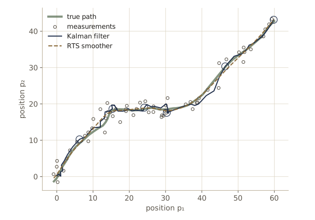
Learning in LDS
When the parameters are unknown we can learn them by maximum likelihood with EM, exactly as for the HMM. The E step runs the filter and smoother with \(\boldsymbol{\theta}^{\text{old}}\) and returns the posterior moments the M step needs:
\[\mathbb{E}[\mathbf{z}_n] = \hat{\boldsymbol{\mu}}_n, \qquad \mathbb{E}[\mathbf{z}_n\mathbf{z}_n^{\mathrm{T}}] = \hat{\mathbf{V}}_n + \hat{\boldsymbol{\mu}}_n\hat{\boldsymbol{\mu}}_n^{\mathrm{T}}, \qquad \mathbb{E}[\mathbf{z}_n\mathbf{z}_{n-1}^{\mathrm{T}}] = \hat{\mathbf{V}}_n\mathbf{J}_{n-1}^{\mathrm{T}} + \hat{\boldsymbol{\mu}}_n\hat{\boldsymbol{\mu}}_{n-1}^{\mathrm{T}},\]the last one from the cross-covariance above. The complete-data log likelihood is a sum of three Gaussian log densities (initial state, transitions, emissions), so \(Q\) splits into three parts, each maximized in closed form. The transition part is a linear regression of \(\mathbf{z}_n\) on \(\mathbf{z}_{n-1}\) in which the data enter only through expected sufficient statistics, and the same holds for the emission part with \(\mathbf{x}_n\) regressed on \(\mathbf{z}_n\). Setting derivatives to zero as in modules 02 and 03 gives
\[\begin{aligned} \boldsymbol{\mu}_0^{\text{new}} &= \mathbb{E}[\mathbf{z}_1], \qquad \mathbf{V}_0^{\text{new}} = \mathbb{E}[\mathbf{z}_1\mathbf{z}_1^{\mathrm{T}}] - \mathbb{E}[\mathbf{z}_1]\mathbb{E}[\mathbf{z}_1]^{\mathrm{T}}, \\ \mathbf{A}^{\text{new}} &= \Big( \sum_{n=2}^{N} \mathbb{E}[\mathbf{z}_n\mathbf{z}_{n-1}^{\mathrm{T}}] \Big) \Big( \sum_{n=2}^{N} \mathbb{E}[\mathbf{z}_{n-1}\mathbf{z}_{n-1}^{\mathrm{T}}] \Big)^{-1}, \\ \boldsymbol{\Gamma}^{\text{new}} &= \frac{1}{N-1} \sum_{n=2}^{N} \Big( \mathbb{E}[\mathbf{z}_n\mathbf{z}_n^{\mathrm{T}}] - \mathbf{A}^{\text{new}}\mathbb{E}[\mathbf{z}_{n-1}\mathbf{z}_n^{\mathrm{T}}] - \mathbb{E}[\mathbf{z}_n\mathbf{z}_{n-1}^{\mathrm{T}}](\mathbf{A}^{\text{new}})^{\mathrm{T}} + \mathbf{A}^{\text{new}}\mathbb{E}[\mathbf{z}_{n-1}\mathbf{z}_{n-1}^{\mathrm{T}}](\mathbf{A}^{\text{new}})^{\mathrm{T}} \Big), \\ \mathbf{C}^{\text{new}} &= \Big( \sum_{n=1}^{N} \mathbf{x}_n\mathbb{E}[\mathbf{z}_n]^{\mathrm{T}} \Big) \Big( \sum_{n=1}^{N} \mathbb{E}[\mathbf{z}_n\mathbf{z}_n^{\mathrm{T}}] \Big)^{-1}, \\ \boldsymbol{\Sigma}^{\text{new}} &= \frac{1}{N} \sum_{n=1}^{N} \Big( \mathbf{x}_n\mathbf{x}_n^{\mathrm{T}} - \mathbf{C}^{\text{new}}\mathbb{E}[\mathbf{z}_n]\mathbf{x}_n^{\mathrm{T}} - \mathbf{x}_n\mathbb{E}[\mathbf{z}_n]^{\mathrm{T}}(\mathbf{C}^{\text{new}})^{\mathrm{T}} + \mathbf{C}^{\text{new}}\mathbb{E}[\mathbf{z}_n\mathbf{z}_n^{\mathrm{T}}](\mathbf{C}^{\text{new}})^{\mathrm{T}} \Big). \end{aligned}\]Compare \(\mathbf{A}^{\text{new}}\) with the least-squares solution \((\sum \mathbf{t}_n\boldsymbol{\phi}_n^{\mathrm{T}})(\sum \boldsymbol{\phi}_n\boldsymbol{\phi}_n^{\mathrm{T}})^{-1}\) for a multi-output regression, and \(\boldsymbol{\Gamma}^{\text{new}}\) with the average squared residual. Bishop §13.3.2 gives the steps (exercises 13.32–13.34).
Watch out. An LDS is not identifiable as it stands. Replace \(\mathbf{z}_n\) by \(\mathbf{T}\mathbf{z}_n\) for any invertible \(\mathbf{T}\), and \(\mathbf{A}\), \(\mathbf{C}\), \(\boldsymbol{\Gamma}\), \(\boldsymbol{\mu}_0\), \(\mathbf{V}_0\) by \(\mathbf{T}\mathbf{A}\mathbf{T}^{-1}\), \(\mathbf{C}\mathbf{T}^{-1}\), \(\mathbf{T}\boldsymbol{\Gamma}\mathbf{T}^{\mathrm{T}}\), \(\mathbf{T}\boldsymbol{\mu}_0\), \(\mathbf{T}\mathbf{V}_0\mathbf{T}^{\mathrm{T}}\): the distribution of the observations does not change. EM will converge to one of these equivalent solutions, so compare learned models through quantities that do not depend on the coordinates (predictions, the eigenvalues of \(\mathbf{A}\)), or fix some parameters, as we do next.
A small example: a scalar AR(1) latent process observed in noise, \(z_n = a z_{n-1} + w_n\) and \(x_n = z_n + v_n\), with \(a = 0.95\), \(\Gamma = 0.5\), \(\Sigma = 1\). We fix \(C = 1\), which removes the scale ambiguity, and learn \(a\), \(\Gamma\), \(\Sigma\), \(\mu_0\), and \(V_0\) from 600 observations, starting far from the truth. The code implements the matrix formulas, so it works for any dimension.
def lds_em(X, A, Gamma, C, Sigma, mu0, V0, n_iter, learn_C=False):
    """EM for a linear dynamical system. Returns the parameters and ln p(X) per iteration."""
    N, history = len(X), []
    for it in range(n_iter):
        mu, V, P, ll = kalman_filter(X, A, Gamma, C, Sigma, mu0, V0)      # E step
        mu_s, V_s, J = rts_smoother(mu, V, P, A)
        history.append(ll)
        Ez = mu_s                                                        # E[z_n]
        Ezz = V_s + np.einsum("ni,nj->nij", mu_s, mu_s)                  # E[z_n z_n^T]
        Ezz1 = (np.einsum("nij,nkj->nik", V_s[1:], J[:-1])               # E[z_n z_{n-1}^T]
                + np.einsum("ni,nj->nij", mu_s[1:], mu_s[:-1]))
        mu0, V0 = Ez[0], Ezz[0] - np.outer(Ez[0], Ez[0])                 # M step
        S10, S00, S11 = Ezz1.sum(0), Ezz[:-1].sum(0), Ezz[1:].sum(0)
        A = np.linalg.solve(S00.T, S10.T).T                              # S10 S00^{-1}
        Gamma = (S11 - A @ S10.T - S10 @ A.T + A @ S00 @ A.T) / (N - 1)
        if learn_C:
            C = np.linalg.solve(Ezz.sum(0).T, (X.T @ Ez).T).T
        Sigma = (X.T @ X - C @ Ez.T @ X - X.T @ Ez @ C.T + C @ Ezz.sum(0) @ C.T) / N
    return A, Gamma, Sigma, mu0, V0, np.array(history)

one = np.eye(1)
Z_ar, X_ar = sample_lds(0.95 * one, 0.5 * one, one, 1.0 * one, np.zeros(1), one, 600,
                        np.random.default_rng(8))
A_l, G_l, S_l, m0_l, V0_l, hist_l = lds_em(X_ar, 0.5 * one, 1.0 * one, one, 2.0 * one,
                                           np.zeros(1), one, n_iter=40)
for it in [0, 1, 5, 20, 39]:
    print(f"iteration {it:2d}: ln p(X) = {hist_l[it]:.3f}")
print("log likelihood never decreased:", bool(np.all(np.diff(hist_l) > -1e-8)))
print(f"learned a = {A_l[0, 0]:.4f} (true 0.95),  Gamma = {G_l[0, 0]:.4f} (true 0.5),  "
      f"Sigma = {S_l[0, 0]:.4f} (true 1.0)")
iteration  0: ln p(X) = -1283.803
iteration  1: ln p(X) = -1122.638
iteration  5: ln p(X) = -1057.870
iteration 20: ln p(X) = -1055.062
iteration 39: ln p(X) = -1054.928
log likelihood never decreased: True
learned a = 0.9577 (true 0.95),  Gamma = 0.4822 (true 0.5),  Sigma = 1.0416 (true 1.0)
The learned values are close to the truth, and the likelihood climbs monotonically. Convergence is slower than for the HMM example; EM for state-space models is often slow when the noise levels are hard to tell apart from the dynamics.
As with the HMM, priors on the parameters give MAP estimates with the same E step, and the variational methods of module 10 give a Bayesian treatment.
Extensions of LDS
The linear-Gaussian assumption buys exact, cheap inference, but it also forces the observations to be jointly Gaussian, which is often wrong. Some extensions keep exactness: a Gaussian-mixture prior for \(\mathbf{z}_1\) with \(K\) components yields filtered distributions that remain \(K\)-component mixtures, since each component is propagated by its own Kalman filter. Others do not: a mixture emission density multiplies the number of components by \(K\) at every step, as we saw above, and any nonlinear dynamics or measurement function makes the filtered distribution non-Gaussian.
For those models there are three broad strategies. The extended Kalman filter (EKF) linearizes the nonlinear functions around the current estimate (a first-order Taylor expansion) and applies the Kalman equations to the linearized model. Assumed density filtering and expectation propagation (module 10) project the exact update back onto a Gaussian by matching moments. Sampling methods, the subject of the next subsection, represent the filtered distribution by a cloud of weighted samples.
We can also combine models, as with the HMM. A switching state-space model has several linear dynamical systems and a discrete Markov chain that selects which of them produces each observation, which can describe, for instance, a target that alternates between cruising and maneuvering. Exact inference is intractable (the number of possible switching histories grows exponentially), but variational methods give an efficient approximation that runs forward–backward passes on the discrete chain and Kalman passes on the continuous ones. Replacing the continuous chains by discrete ones gives the analogous switching HMM.
Particle filters
For a state-space model that is not linear-Gaussian, the filtered distribution has no closed form, but we can still sample from it. The particle filter applies the sampling–importance–resampling idea of module 11 one time step at a time.
Write \(\mathbf{X}_n = (\mathbf{x}_1, \dots, \mathbf{x}_n)\). Suppose we have \(L\) samples \(\mathbf{z}_n^{(l)}\), called particles, drawn from the predictive distribution \(p(\mathbf{z}_n \mid \mathbf{X}_{n-1})\). Bayes’ theorem, with the fact that \(\mathbf{x}_n\) depends on the past only through \(\mathbf{z}_n\), turns them into an approximation of the filtered distribution. For any function \(f\),
\[\mathbb{E}[f(\mathbf{z}_n) \mid \mathbf{X}_n] = \frac{\int f(\mathbf{z}_n) \, p(\mathbf{x}_n \mid \mathbf{z}_n) \, p(\mathbf{z}_n \mid \mathbf{X}_{n-1}) \, d\mathbf{z}_n}{\int p(\mathbf{x}_n \mid \mathbf{z}_n) \, p(\mathbf{z}_n \mid \mathbf{X}_{n-1}) \, d\mathbf{z}_n} \approx \sum_{l=1}^{L} w_n^{(l)} f(\mathbf{z}_n^{(l)}), \qquad w_n^{(l)} = \frac{p(\mathbf{x}_n \mid \mathbf{z}_n^{(l)})}{\sum_{m=1}^{L} p(\mathbf{x}_n \mid \mathbf{z}_n^{(m)})}.\]This is importance sampling with the predictive distribution as the proposal: each particle is weighted by how well it explains the new observation. So the filtered distribution is represented by the weighted particles \(\{\mathbf{z}_n^{(l)}, w_n^{(l)}\}\).
To move to the next step we need samples from \(p(\mathbf{z}_{n+1} \mid \mathbf{X}_n)\). Since \(\mathbf{z}_{n+1}\) depends on the past only through \(\mathbf{z}_n\),
\[p(\mathbf{z}_{n+1} \mid \mathbf{X}_n) = \int p(\mathbf{z}_{n+1} \mid \mathbf{z}_n) \, p(\mathbf{z}_n \mid \mathbf{X}_n) \, d\mathbf{z}_n \approx \sum_{l=1}^{L} w_n^{(l)} \, p(\mathbf{z}_{n+1} \mid \mathbf{z}_n^{(l)}),\]a mixture with one component per particle. We sample from it the usual way for mixtures: choose a particle \(l\) with probability \(w_n^{(l)}\) (this is resampling), then draw from the transition density from that particle.
Definition. The bootstrap particle filter. Draw \(L\) particles from \(p(\mathbf{z}_1)\). Then, for \(n = 1, 2, \dots\): (1) weight each particle by \(p(\mathbf{x}_n \mid \mathbf{z}_n^{(l)})\) and normalize; (2) resample \(L\) particles with probabilities \(w_n^{(l)}\); (3) propagate each through the dynamics, \(\mathbf{z}_{n+1}^{(l)} \sim p(\mathbf{z}_{n+1} \mid \mathbf{z}_n^{(l)})\).
The algorithm needs only two things from the model: a way to sample the dynamics and a way to evaluate the emission density. The average unnormalized weight, \(\frac{1}{L}\sum_l p(\mathbf{x}_n \mid \mathbf{z}_n^{(l)})\), estimates the predictive probability \(c_n = p(\mathbf{x}_n \mid \mathbf{X}_{n-1})\), so the filter also estimates the log likelihood. We compute the weights in log space, for the same reason as always.
def bootstrap_pf(X, sample_z1, sample_trans, log_emit, L, rng):
    """Bootstrap particle filter. sample_z1(L, rng) -> (L, D) particles;
    sample_trans(z, n, rng) propagates particles to step n (0-based); log_emit(x, z) -> (L,).
    Returns the filtered means (N, D) and the estimate of ln p(X)."""
    N = len(X)
    z = sample_z1(L, rng)
    means, loglik = [], 0.0
    for n in range(N):
        if n > 0:
            idx = rng.choice(L, size=L, p=w)                 # resample: pick mixture components
            z = sample_trans(z[idx], n, rng)                 # propagate through the dynamics
        logw = log_emit(X[n], z)                             # weight by the new observation
        m = logsumexp(logw)
        loglik += m - np.log(L)                              # ln of the average weight ~ ln c_n
        w = np.exp(logw - m)
        means.append(w @ z)
    return np.array(means), loglik
On the linear tracking problem the Kalman filter is exact, so it is a perfect reference. We give the particle filter the same model and compare its filtered means and log likelihood with the Kalman filter’s as the number of particles grows.
L_Gamma, L_V0 = np.linalg.cholesky(Gamma_cv), np.linalg.cholesky(V0_cv)
lin_z1 = lambda L, rng: mu0_cv + rng.standard_normal((L, 4)) @ L_V0.T
lin_trans = lambda z, n, rng: z @ A_cv.T + rng.standard_normal(z.shape) @ L_Gamma.T
def lin_emit(x, z):
    d = x - z[:, :2]
    return -0.5 * np.sum(d**2, axis=1) / Sigma_cv[0, 0] - np.log(2 * np.pi * Sigma_cv[0, 0])

print(f"Kalman filter:  ln p(X) = {ll_trk:.2f}, RMS error {rms(mu_f[:, :2] - pos):.3f}")
for L in [100, 1000, 10000]:
    m_pf, ll_pf = bootstrap_pf(X_trk, lin_z1, lin_trans, lin_emit, L,
                               np.random.default_rng(1))
    print(f"PF, L = {L:5d}: ln p(X) = {ll_pf:.2f}, RMS error {rms(m_pf[:, :2] - pos):.3f}, "
          f"distance to Kalman means {rms(m_pf[:, :2] - mu_f[:, :2]):.3f}")
Kalman filter:  ln p(X) = -247.57, RMS error 1.231
PF, L =   100: ln p(X) = -261.23, RMS error 1.604, distance to Kalman means 1.180
PF, L =  1000: ln p(X) = -247.12, RMS error 1.235, distance to Kalman means 0.340
PF, L = 10000: ln p(X) = -245.87, RMS error 1.205, distance to Kalman means 0.117
With 100 particles the particle filter is a poor approximation: its means are further from the truth than the Kalman filter’s, and its log likelihood is off by more than 10. With 10,000 its means are close to the Kalman means and its log likelihood is within a couple of units of the exact value. The distance to the Kalman means drops by roughly a factor of 3 for each tenfold increase in \(L\), in line with the \(\sqrt{10} \approx 3.2\) expected of Monte Carlo error, which shrinks like \(1/\sqrt{L}\); each extra digit of accuracy costs a hundred times more particles. Where the Kalman filter applies, use it.
The particle filter earns its keep when the model is nonlinear. A standard one-dimensional test problem from the particle-filtering literature has strongly nonlinear dynamics and a measurement of the square of the state:
\[z_n = \frac{z_{n-1}}{2} + \frac{25 z_{n-1}}{1 + z_{n-1}^2} + 8\cos(1.2 n) + w_n, \qquad x_n = \frac{z_n^2}{20} + v_n,\]with \(w_n \sim \mathcal{N}(0, 10)\), \(v_n \sim \mathcal{N}(0, 1)\), and \(z_1 \sim \mathcal{N}(0, 5)\). Because the measurement cannot tell \(z\) from \(-z\), the filtered distribution is often bimodal, which no single Gaussian can represent. We compare the particle filter with an extended Kalman filter, which linearizes the dynamics with the derivative \(f'(z) = \frac{1}{2} + 25\frac{1 - z^2}{(1 + z^2)^2}\) and the measurement with \(h'(z) = z/10\).
q_ng, r_ng = 10.0, 1.0
def f_ng(z, t):                                  # dynamics at time t (1-based)
    return z / 2 + 25 * z / (1 + z**2) + 8 * np.cos(1.2 * t)
def df_ng(z):
    return 0.5 + 25 * (1 - z**2) / (1 + z**2)**2

def sample_ng(N, rng):
    z = np.empty(N)
    z[0] = rng.normal(0, np.sqrt(5.0))
    for n in range(1, N):
        z[n] = f_ng(z[n - 1], n + 1) + rng.normal(0, np.sqrt(q_ng))
    return z, z**2 / 20 + rng.normal(0, np.sqrt(r_ng), N)

def ekf_ng(x, m0=0.0, P0=5.0):
    """Extended Kalman filter for the model above (scalar state)."""
    m, P, out = m0, P0, []
    for n in range(len(x)):
        if n > 0:                                 # predict, linearizing f at the current mean
            F = df_ng(m)
            m, P = f_ng(m, n + 1), F * P * F + q_ng
        H = m / 10                                # linearize h(z) = z^2 / 20
        S = H * P * H + r_ng
        k = P * H / S
        m, P = m + k * (x[n] - m**2 / 20), (1 - k * H) * P
        out.append(m)
    return np.array(out)

ng_z1 = lambda L, rng: rng.normal(0, np.sqrt(5.0), (L, 1))
ng_trans = lambda z, n, rng: f_ng(z, n + 1) + rng.normal(0, np.sqrt(q_ng), z.shape)
ng_emit = lambda x, z: -0.5 * (x - z[:, 0]**2 / 20)**2 / r_ng

err = []
for seed in range(20):                            # 20 independent sequences of length 60
    z_ng, x_ng = sample_ng(60, np.random.default_rng(seed))
    m_ekf = ekf_ng(x_ng)
    m_pf, _ = bootstrap_pf(x_ng, ng_z1, ng_trans, ng_emit, 2000,
                           np.random.default_rng(100 + seed))
    err.append([np.sqrt(np.mean((m_ekf - z_ng)**2)),
                np.sqrt(np.mean((m_pf[:, 0] - z_ng)**2))])
err = np.array(err)
print(f"RMS error over 20 sequences: EKF mean {err[:, 0].mean():.2f}, "
      f"particle filter (L = 2000) mean {err[:, 1].mean():.2f}")
print(f"particle filter better on {np.sum(err[:, 1] < err[:, 0])} of 20 sequences")
RMS error over 20 sequences: EKF mean 20.90, particle filter (L = 2000) mean 4.43
particle filter better on 20 of 20 sequences
The extended Kalman filter fails badly here: its single Gaussian regularly locks onto the wrong sign of \(z\) and cannot recover. The particle filter keeps particles on both sides until the dynamics resolve the ambiguity. Its error is smaller on all 20 sequences, and on average it is less than a quarter of the EKF’s.
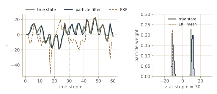
In practice. The weakness of particle filters is weight degeneracy: when the likelihood is sharp compared with the spread of the predicted particles, a few particles take nearly all the weight and the rest are wasted. Useful remedies are resampling only when the effective sample size \(1 / \sum_l (w^{(l)})^2\) drops below a threshold, lower-variance resampling schemes such as systematic resampling (exercise 11), and proposals that look at the new observation instead of sampling blindly from the dynamics. The number of particles needed also grows quickly with the dimension of the state, so particle filters are at their best for low-dimensional states with awkward, non-Gaussian posteriors.
The same algorithm has been published under several names, including the bootstrap filter, sequential Monte Carlo, and the condensation algorithm in computer vision.
Summary
| Model | Latent variables | Inference | Learning |
|---|---|---|---|
| Markov chain, order \(M\) | none | none needed | counting (\(K^M(K-1)\) parameters) or regression (AR model) |
| Hidden Markov model | discrete, \(K\) states | forward–backward for \(\gamma\), \(\xi\), \(p(\mathbf{X})\) in \(O(K^2N)\); Viterbi for the best path | EM (Baum–Welch) |
| Linear dynamical system | Gaussian | Kalman filter, RTS smoother, \(O(N)\) | EM with expected sufficient statistics |
| Nonlinear or non-Gaussian state-space model | any | particle filter (sampling), EKF or moment matching (approximate) | EM or Bayesian methods with approximate E steps |
Ideas to carry forward:
- Latent variables that form a Markov chain give observations with long-range dependence from a few parameters. The graph is a tree, so exact inference is message passing along the chain, linear in its length.
- The forward pass is filtering, the backward pass turns filtering into smoothing, and the likelihood is the product of the one-step predictive probabilities \(c_n\). The HMM and the LDS run the same algorithm with sums or with Gaussian integrals.
- Numerical care is part of the algorithm: normalize the forward messages (or work in logs), and use linear solves rather than inverses.
- Learning is EM, and the E step needs only single-step and neighboring-pair posteriors. Hidden states are identified only up to relabeling (HMM) or a change of coordinates (LDS).
Exercises
- Construct a two-state HMM with discrete emissions (two symbols) and compute, by brute-force enumeration of the latent states, \(p(x_3 \mid x_1, x_2)\) and \(p(x_3 \mid x_2)\) for all settings of \(x_1, x_2, x_3\). Show that they differ, so the observations are not a first-order Markov chain. Can you choose parameters for which they are equal? What does that say about the model?
- Derive the M-step updates for \(\boldsymbol{\pi}\) and \(\mathbf{A}\) with Lagrange multipliers, as in the module, and prove that if \(A_{jk} = 0\) before an EM iteration, then \(A_{jk} = 0\) after it. Use this to train a three-state left-to-right HMM with
baum_welchon sequences sampled from a left-to-right model, and confirm that the lower triangle of \(\mathbf{A}\) stays zero. - Rewrite
baum_welchfor discrete emissions with \(D\) symbols (emission table \(\mu_{ik}\)). Test it on data from a two-state model in which one state emits the six faces of a die uniformly and the other favors one face, and report the fitted table against the true one. - Build a three-state HMM whose transition matrix has a zero, together with an observation sequence, for which the per-step most probable states from \(\gamma\) form a path of probability zero. Verify with
forward_backward,viterbi, andpath_log_joint. - Show that \(\sum_{k} \xi(z_{n-1,j}, z_{nk}) = \gamma(z_{n-1,j})\) for every \(n\) and \(j\), first from the definitions and then from the scaled formulas. Why does this identity make a good unit test for a forward–backward implementation?
- Extend
forward_backwardand the prediction code to compute \(p(\mathbf{x}_{N+1} \mid \mathbf{X})\) for each \(N\) along the length-1000 sequence, using the scaled forward variables. Check that \(\sum_n \ln p(\mathbf{x}_n \mid \mathbf{x}_1, \dots, \mathbf{x}_{n-1})\) equals the log likelihood. - For the scalar random walk of the module, find the steady-state predicted variance \(P\) and gain \(k\) in closed form as functions of \(q\) and \(r\). Show that \(k \to 1\) as \(q/r \to \infty\) and that \(k \approx \sqrt{q/r}\) as \(q/r \to 0\), and compare with the printed values.
- Add known offsets to the LDS, \(\mathbf{z}_n = \mathbf{A}\mathbf{z}_{n-1} + \mathbf{a} + \mathbf{w}_n\) and \(\mathbf{x}_n = \mathbf{C}\mathbf{z}_n + \mathbf{c} + \mathbf{v}_n\). Derive the changes to the Kalman filter and the RTS smoother, implement them, and test them by tracking an object that falls under constant gravity.
- Show that for an LDS the posterior mode of \(p(\mathbf{Z} \mid \mathbf{X})\) equals the sequence of smoothed means. Then verify it numerically for the 60-step track: write \(\ln p(\mathbf{X}, \mathbf{Z})\) as a quadratic in the stacked \(\mathbf{Z}\), maximize it by solving one linear system, and compare with
mu_sm. - Run
lds_emon the scalar example withlearn_C=True. Show that the learned log likelihood is as good as with \(C\) fixed, but that \(C\), \(\Gamma\), and \(V_0\) are different; check that they are related to the fixed-\(C\) solution by a rescaling of \(z\), up to EM’s convergence. - Implement systematic resampling (one uniform draw \(u \sim \mathcal{U}(0, 1/L)\), then pick the particles at the positions \(u + (l-1)/L\) of the cumulative weights) and resampling only when the effective sample size falls below \(L/2\). Over 50 runs with \(L = 1000\) on the tracking problem, compare the standard deviation of the log likelihood estimate for the three schemes.
- In your own words: explain to a classmate what the forward variable, the Kalman filter’s mean and covariance, and a set of weighted particles have in common, and why each can be updated with a new observation without looking back at the old ones.
Going further
- C. M. Bishop, Pattern Recognition and Machine Learning, chapter 13. Exercises 13.5–13.8 derive the M-step equations, 13.12 covers multiple training sequences, 13.16 derives the Viterbi recursion, 13.19 shows why the LDS needs no Viterbi algorithm, 13.24 adds offsets to the LDS, 13.27–13.29 study limits of the Kalman filter and derive the smoother from the backward recursion, and 13.32–13.34 verify the LDS M-step equations.
- L. R. Rabiner, “A tutorial on hidden Markov models and selected applications in speech recognition”, Proceedings of the IEEE, 1989 — the classic introduction to HMMs, with scaling, left-to-right models, and duration modeling.
- R. E. Kalman, “A new approach to linear filtering and prediction problems”, Journal of Basic Engineering, 1960 — the original Kalman filter paper.
- H. E. Rauch, F. Tung, and C. T. Striebel, “Maximum likelihood estimates of linear dynamic systems”, AIAA Journal, 1965 — the RTS smoother.
- N. J. Gordon, D. J. Salmond, and A. F. M. Smith, “Novel approach to nonlinear/non-Gaussian Bayesian state estimation”, IEE Proceedings F, 1993 — the bootstrap particle filter.
- S. Särkkä, Bayesian Filtering and Smoothing (Cambridge University Press, 2013) — a clear, modern textbook on Kalman filters, smoothers, extended and unscented filters, and particle methods, written for readers at the level of this course.
These notes follow the chapters of C. M. Bishop, Pattern Recognition and Machine Learning (Springer, 2006), the course text, which Microsoft Research makes freely available as a PDF. The explanations, code, figures, and exercises here are written for this course; the book remains the reference, with the full derivations and many more exercises.