CSE 474/574 · Module 03 · Week 3
Linear Models for Regression
Basis functions and least squares, regularization, the bias–variance decomposition, Bayesian linear regression, and the evidence approximation.
Companion reading: Bishop, Pattern Recognition and Machine Learning, chapter 3, “Linear Models for Regression”
By the end of this module you can
- Build a design matrix from polynomial, Gaussian, or sigmoidal basis functions, and fit the weights by maximum likelihood with a numerically sound least-squares solver.
- Derive the normal equations, the maximum likelihood noise precision, and the role of the bias parameter, and explain least squares as an orthogonal projection.
- Fit a model sequentially with the LMS rule, and say why the learning rate decides whether it converges to the batch solution.
- Derive the ridge solution, explain why the lasso produces sparse weights, and solve the lasso by coordinate descent.
- Derive the bias–variance decomposition of the expected squared loss and measure bias, variance, and test error in a simulation.
- Derive the Gaussian posterior over the weights and the predictive distribution of Bayesian linear regression, update them one data point at a time, and read off the equivalent kernel.
- Explain what the model evidence measures, why it penalizes needless complexity, and compute it in closed form for a linear-Gaussian model.
- Choose the hyperparameters α and β by maximizing the evidence, and interpret the effective number of parameters γ.
Contents
- Linear basis function models
- From linear regression to basis functions
- Choices of basis function
- Maximum likelihood and least squares
- Solving the normal equations in practice
- The bias parameter and the noise precision
- The geometry of least squares
- Sequential learning
- Regularized least squares
- The lasso and the q-norm family
- Multiple outputs
- The bias–variance decomposition
- Bayesian linear regression
- Bayesian model comparison
- The evidence approximation
- Limitations of fixed basis functions
- Summary
- Exercises
- Going further
In module 01 we fitted polynomials to noisy samples of \(\sin(2\pi x)\). We saw that a least-squares fit is the maximum likelihood solution under Gaussian noise, that a flexible model overfits a small data set, and that adding a penalty on the size of the weights (ridge regression) tames the overfitting. In module 02 we worked out the algebra of the Gaussian: conditionals, marginals, and the rules for a linear-Gaussian model, where one Gaussian variable depends linearly on another.
This module puts those pieces together into a complete treatment of linear regression models: models whose output is a linear function of the adjustable parameters, even though it may be a very nonlinear function of the input. That single property, linearity in the parameters, makes almost everything computable in closed form. We get the maximum likelihood solution by solving a linear system, the Bayesian posterior over the weights is exactly Gaussian, and even the quantity that Bayesian model comparison needs, the probability of the data under a model, has a formula.
We follow Bishop’s chapter 3 in order. First the frequentist toolkit: basis functions, least squares, its geometry, sequential fitting, and regularization. Then the bias–variance decomposition, which explains overfitting as a trade-off between two kinds of error. Then the Bayesian treatment: posterior, predictive distribution, and the equivalent kernel. Finally, Bayesian model comparison and the evidence approximation, which choose the model complexity from the training data alone. The last section explains why these models are not the end of the story, which motivates neural networks and kernel methods in modules 05–07.
Linear basis function models
From linear regression to basis functions
The simplest regression model for an input vector \(\mathbf{x} = (x_1, \dots, x_D)^{\mathrm{T}}\) is a weighted sum of its components plus a constant,
\[y(\mathbf{x}, \mathbf{w}) = w_0 + w_1 x_1 + \dots + w_D x_D .\]It is linear in the weights, which is what makes it easy to fit, but it is also linear in the inputs, which makes it too rigid for most problems: it cannot even represent a parabola. The fix is to keep the linearity in the weights but feed the model fixed nonlinear transformations of the input. Choose \(M - 1\) functions \(\phi_1(\mathbf{x}), \dots, \phi_{M-1}(\mathbf{x})\) and write
\[y(\mathbf{x}, \mathbf{w}) = w_0 + \sum_{j=1}^{M-1} w_j \phi_j(\mathbf{x}) .\]The \(\phi_j\) are called basis functions, and a model of this form is a linear basis function model. The constant \(w_0\) lets the model shift its output up or down by a fixed amount; it is called the bias parameter (a different use of the word “bias” from the statistical one we meet in the bias–variance section). To tidy the notation we add a dummy basis function \(\phi_0(\mathbf{x}) = 1\), collect the basis functions into a vector \(\boldsymbol{\phi}(\mathbf{x}) = (\phi_0(\mathbf{x}), \dots, \phi_{M-1}(\mathbf{x}))^{\mathrm{T}}\) and the weights into \(\mathbf{w} = (w_0, \dots, w_{M-1})^{\mathrm{T}}\), and write
\[y(\mathbf{x}, \mathbf{w}) = \sum_{j=0}^{M-1} w_j \phi_j(\mathbf{x}) = \mathbf{w}^{\mathrm{T}} \boldsymbol{\phi}(\mathbf{x}) .\]So the model has \(M\) parameters in all. The model can bend and curve in \(\mathbf{x}\) as much as its basis functions do, yet as a function of \(\mathbf{w}\) it is a plain dot product. Choosing the basis functions is a form of feature extraction: \(\boldsymbol{\phi}(\mathbf{x})\) is a fixed, hand-designed representation of the raw input, and the learning happens only in the weights on top of it.
The polynomial of module 01 is the special case \(\phi_j(x) = x^j\) with a single input \(x\). Most of this module works for any choice of basis, including the identity \(\boldsymbol{\phi}(\mathbf{x}) = \mathbf{x}\) (with a bias), so we write the theory for a general \(\boldsymbol{\phi}\) and pick a concrete basis only when we compute.
Choices of basis function
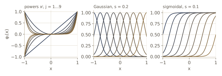
Three families come up again and again, all shown in the figure below.
- Polynomials, \(\phi_j(x) = x^j\). Their weakness is that they are global: each one is nonzero almost everywhere, so moving one weight changes the fit over the whole input range, and a change needed in one region disturbs every other region. Splitting the input range into pieces and fitting a separate low-order polynomial in each gives splines, which avoid this.
- Gaussian basis functions, \(\phi_j(x) = \exp\left(-\frac{(x - \mu_j)^2}{2 s^2}\right)\). Each is a bump centered at \(\mu_j\) with width set by \(s\). They are local: \(\phi_j\) is essentially zero far from \(\mu_j\). Despite the name there is nothing probabilistic here, and no normalizing constant is needed because each bump is multiplied by a free weight anyway.
- Sigmoidal basis functions, \(\phi_j(x) = \sigma\left(\frac{x - \mu_j}{s}\right)\), where \(\sigma(a) = \frac{1}{1 + e^{-a}}\) is the logistic sigmoid. Each is a smooth step from 0 to 1 located at \(\mu_j\). Because \(\tanh(a) = 2\sigma(2a) - 1\), a tanh step of width \(s\) is a logistic step of width \(s/2\), doubled and shifted down by 1; so a linear combination of tanh steps can always be rewritten as a linear combination of logistic steps, with doubled weights and a different bias.
Other choices matter in other fields. A Fourier basis of sines and cosines gives each basis function one frequency and infinite extent; wavelets are localized in both position and frequency, and are widely used for signals and images sampled on a regular grid.
Here is the code we use throughout. A design matrix \(\mathbf{\Phi}\) holds the basis functions evaluated at the training inputs: row \(n\) is \(\boldsymbol{\phi}(\mathbf{x}_n)^{\mathrm{T}}\), so \(\Phi_{nj} = \phi_j(\mathbf{x}_n)\) and \(\mathbf{\Phi}\) has shape \(N \times M\). Our design_matrix always puts the constant column \(\phi_0 = 1\) first.
import numpy as np
from scipy.special import expit, logsumexp      # expit is the logistic sigmoid
from scipy.linalg import cho_factor, cho_solve, solve_triangular

np.set_printoptions(precision=4, suppress=True)
rng = np.random.default_rng(3)

NOISE_SD = 0.3                 # standard deviation of the target noise
BETA_TRUE = 1 / NOISE_SD**2    # the true noise precision, about 11.1

def sin_data(N, seed, noise_sd=NOISE_SD):
    """N inputs uniform on [0, 1] and targets sin(2 pi x) + Gaussian noise."""
    g = np.random.default_rng(seed)
    x = g.uniform(0, 1, N)
    t = np.sin(2 * np.pi * x) + g.normal(0, noise_sd, N)
    return x, t

def poly_basis(x, M):
    """Columns x, x^2, ..., x^M."""
    return x[:, None] ** np.arange(1, M + 1)

def gauss_basis(x, mu, s):
    """Columns exp(-(x - mu_j)^2 / (2 s^2)), one per center mu_j."""
    return np.exp(-(x[:, None] - mu[None, :]) ** 2 / (2 * s**2))

def sigmoid_basis(x, mu, s):
    """Columns sigma((x - mu_j) / s), one per center mu_j."""
    return expit((x[:, None] - mu[None, :]) / s)

def design_matrix(x, basis, *args):
    """N x M design matrix: a column of ones (phi_0 = 1), then basis(x, *args)."""
    return np.column_stack([np.ones(len(x)), basis(x, *args)])

a = np.linspace(-3, 3, 7)
print("tanh(a) = 2 sigma(2a) - 1:", np.allclose(np.tanh(a), 2 * expit(2 * a) - 1))

x, t = sin_data(25, seed=1)                      # the running data set
MU9, S9 = np.linspace(0, 1, 9), 0.1              # 9 Gaussian bumps on [0, 1]
Phi = design_matrix(x, gauss_basis, MU9, S9)
print("Phi shape:", Phi.shape)
print("first row:", Phi[0])
tanh(a) = 2 sigma(2a) - 1: True
Phi shape: (25, 10)
first row: [1.     0.     0.0006 0.0325 0.3922 0.993  0.527  0.0586 0.0014 0.    ]
The running data set has \(N = 25\) points, and the model has nine Gaussian bumps plus the bias, so \(M = 10\). The first row shows the locality of the Gaussian basis: for an input near 0.5, only the bumps centered near 0.5 are awake.
Maximum likelihood and least squares
We assume, as in module 01, that each target is a deterministic function of the input plus Gaussian noise,
\[t = y(\mathbf{x}, \mathbf{w}) + \epsilon, \qquad \epsilon \sim \mathcal{N}(0, \beta^{-1}),\]where \(\beta\) is the noise precision (inverse variance). Equivalently, \(p(t \mid \mathbf{x}, \mathbf{w}, \beta) = \mathcal{N}(t \mid y(\mathbf{x}, \mathbf{w}), \beta^{-1})\). Under squared loss the best prediction for a new input is the conditional mean \(\mathbb{E}[t \mid \mathbf{x}] = y(\mathbf{x}, \mathbf{w})\) (module 01’s decision theory). The assumption has a cost worth naming: this conditional distribution has a single peak, so the model cannot describe a target that takes one of two quite different values for the same input. Mixture models for such cases come in modules 05 and 14.
Take \(N\) inputs \(\mathbf{x}_1, \dots, \mathbf{x}_N\) with targets collected in the column vector \(\mathbf{t} = (t_1, \dots, t_N)^{\mathrm{T}}\), drawn independently. In regression we never model the inputs themselves, so we drop them from the conditioning to keep the notation light. The likelihood is a product of Gaussians, and its logarithm is
\[\begin{aligned} \ln p(\mathbf{t} \mid \mathbf{w}, \beta) &= \sum_{n=1}^{N} \ln \mathcal{N}\left(t_n \mid \mathbf{w}^{\mathrm{T}} \boldsymbol{\phi}(\mathbf{x}_n), \beta^{-1}\right) \\ &= \frac{N}{2} \ln \beta - \frac{N}{2} \ln (2\pi) - \beta E_D(\mathbf{w}), \end{aligned}\]with the sum-of-squares error
\[E_D(\mathbf{w}) = \frac{1}{2} \sum_{n=1}^{N} \left\{ t_n - \mathbf{w}^{\mathrm{T}} \boldsymbol{\phi}(\mathbf{x}_n) \right\}^2 = \frac{1}{2} \lVert \mathbf{t} - \mathbf{\Phi} \mathbf{w} \rVert^2 .\]Only the last term depends on \(\mathbf{w}\), so maximizing the likelihood over \(\mathbf{w}\) is the same as minimizing \(E_D\): under Gaussian noise, maximum likelihood is least squares. To find the minimum, set the gradient to zero. In matrix form,
\[\nabla_{\mathbf{w}} E_D = -\mathbf{\Phi}^{\mathrm{T}} (\mathbf{t} - \mathbf{\Phi} \mathbf{w}) = \mathbf{0} \quad\Longrightarrow\quad \mathbf{\Phi}^{\mathrm{T}} \mathbf{\Phi} \, \mathbf{w} = \mathbf{\Phi}^{\mathrm{T}} \mathbf{t} .\]These \(M\) linear equations are the normal equations. When \(\mathbf{\Phi}^{\mathrm{T}} \mathbf{\Phi}\) is invertible (the columns of \(\mathbf{\Phi}\) are linearly independent, which needs \(N \ge M\)), the solution is
\[\mathbf{w}_{\mathrm{ML}} = \left(\mathbf{\Phi}^{\mathrm{T}} \mathbf{\Phi}\right)^{-1} \mathbf{\Phi}^{\mathrm{T}} \mathbf{t} = \mathbf{\Phi}^{\dagger} \mathbf{t}, \qquad \mathbf{\Phi}^{\dagger} \equiv \left(\mathbf{\Phi}^{\mathrm{T}} \mathbf{\Phi}\right)^{-1} \mathbf{\Phi}^{\mathrm{T}} .\]The \(M \times N\) matrix \(\mathbf{\Phi}^{\dagger}\) is the Moore–Penrose pseudo-inverse of \(\mathbf{\Phi}\). It plays the role of an inverse for a tall matrix: \(\mathbf{\Phi}^{\dagger} \mathbf{\Phi} = \mathbf{I}\), and when \(\mathbf{\Phi}\) is square and invertible, \(\mathbf{\Phi}^{\dagger} = \mathbf{\Phi}^{-1}\).
Three ways to compute the same thing:
def fit_ml(Phi, t):
    """Least-squares / maximum likelihood weights via an orthogonal-factorization solver."""
    w, *_ = np.linalg.lstsq(Phi, t, rcond=None)
    return w

w_ml = fit_ml(Phi, t)
w_normal = np.linalg.solve(Phi.T @ Phi, Phi.T @ t)     # the normal equations
w_pinv = np.linalg.pinv(Phi) @ t                        # the pseudo-inverse (via the SVD)

print("w_ML:", w_ml)
print(f"max difference, normal equations vs lstsq: {np.max(np.abs(w_normal - w_ml)):.2e}")
print(f"max difference, pinv vs lstsq:             {np.max(np.abs(w_pinv - w_ml)):.2e}")
print(f"cond(Phi) = {np.linalg.cond(Phi):.1f},  cond(Phi^T Phi) = {np.linalg.cond(Phi.T @ Phi):.1f}")
w_ML: [ 3.2747 -2.386  -0.7668 -1.7872 -0.2652 -2.8849 -0.5621 -2.6119 -2.2448
 -1.6955]
max difference, normal equations vs lstsq: 2.10e-12
max difference, pinv vs lstsq:             5.77e-15
cond(Phi) = 337.3,  cond(Phi^T Phi) = 113787.9
The three answers agree to many digits here. Notice the weights, though. The bias is about 3.3 and almost every bump weight is negative, down to about \(-2.9\): the bias lifts the whole curve and the bumps pull it back down, although the targets themselves stay within about \(\pm 1.5\). Nine overlapping bumps added together look much like a constant, so the bias column and the sum of the bump columns are nearly interchangeable, and the fit trades one against the other. That is a small sign of the numerical trouble discussed next.
Solving the normal equations in practice
The condition number of a matrix, the ratio of its largest to smallest singular value, measures how much relative error in the data can be amplified in the solution of a linear system; roughly, a condition number of \(10^k\) costs \(k\) of the 16 decimal digits that double precision carries. The trouble with the normal equations is that forming \(\mathbf{\Phi}^{\mathrm{T}} \mathbf{\Phi}\) squares the condition number of \(\mathbf{\Phi}\). Solvers such as np.linalg.lstsq work on \(\mathbf{\Phi}\) directly, through an orthogonal factorization or the singular value decomposition, and only pay for the condition number of \(\mathbf{\Phi}\) itself.
Polynomials on \([0, 1]\) make this vivid, because \(x^8\) and \(x^9\) look almost the same on that interval. In the next cell we take polynomials of degree 5, 9, and 13, choose true weights, compute noise-free targets, and ask both methods to recover the weights exactly.
xg = np.linspace(0, 1, 50)
g = np.random.default_rng(0)
print("deg  cond(Phi)  cond(Phi^T Phi)  error(normal eq.)  error(lstsq)")
for M in [5, 9, 13]:
    P = design_matrix(xg, poly_basis, M)
    w_true = g.normal(size=M + 1)
    tt = P @ w_true                                   # exact targets, no noise
    err_ne = np.max(np.abs(np.linalg.solve(P.T @ P, P.T @ tt) - w_true))
    err_ls = np.max(np.abs(fit_ml(P, tt) - w_true))
    print(f"{M:3d}  {np.linalg.cond(P):9.1e}   {np.linalg.cond(P.T @ P):9.1e}"
          f"        {err_ne:9.1e}       {err_ls:9.1e}")
deg  cond(Phi)  cond(Phi^T Phi)  error(normal eq.)  error(lstsq)
  5    3.5e+03     1.3e+07          2.0e-11         3.8e-14
  9    3.6e+06     1.3e+13          1.9e-04         5.2e-11
 13    4.0e+09     6.6e+17          5.4e-01         2.6e-08
The second column is the square of the first, and the error of the normal equations grows with it, reaching about 0.5 for degree 13 while lstsq still recovers the weights well. The lesson for practice: never form \((\mathbf{\Phi}^{\mathrm{T}} \mathbf{\Phi})^{-1}\) explicitly, and prefer lstsq (or a QR factorization) for plain least squares. As we will see shortly, adding a regularizer also cures the problem, because it pushes all the eigenvalues of the system matrix away from zero.
In practice. Scale and center your inputs before building polynomial features, choose Gaussian widths comparable to the spacing of their centers rather than much wider, and use
lstsqor a Cholesky solve of a regularized system. Each of these keeps the condition number, and so the lost digits, under control.
The bias parameter and the noise precision
The bias weight has a simple interpretation. Write it out separately in the error, \(E_D = \frac{1}{2} \sum_n \{ t_n - w_0 - \sum_{j \ge 1} w_j \phi_j(\mathbf{x}_n) \}^2\), and set the derivative with respect to \(w_0\) to zero. Dividing by \(N\) gives
\[w_0 = \bar{t} - \sum_{j=1}^{M-1} w_j \bar{\phi}_j, \qquad \bar{t} = \frac{1}{N} \sum_{n=1}^{N} t_n, \quad \bar{\phi}_j = \frac{1}{N} \sum_{n=1}^{N} \phi_j(\mathbf{x}_n).\]The bias makes up the difference between the average target and the average of what the other basis functions predict. The residuals of a least-squares fit with a bias therefore average exactly to zero.
The noise precision comes from maximizing the log likelihood over \(\beta\) with \(\mathbf{w} = \mathbf{w}_{\mathrm{ML}}\) fixed. The derivative of \(\frac{N}{2} \ln \beta - \beta E_D\) is \(\frac{N}{2\beta} - E_D\), so
\[\frac{1}{\beta_{\mathrm{ML}}} = \frac{1}{N} \sum_{n=1}^{N} \left\{ t_n - \mathbf{w}_{\mathrm{ML}}^{\mathrm{T}} \boldsymbol{\phi}(\mathbf{x}_n) \right\}^2 ,\]the mean squared residual.
phibar = Phi[:, 1:].mean(axis=0)
w0_formula = t.mean() - w_ml[1:] @ phibar
print(f"w0 from lstsq: {w_ml[0]:.4f}   w0 from the averages: {w0_formula:.4f}")

resid = t - Phi @ w_ml
beta_ml = 1 / np.mean(resid**2)
print(f"mean residual: {resid.mean():.1e}")
print(f"beta_ML = {beta_ml:.2f}   (true beta = {BETA_TRUE:.2f})")
w0 from lstsq: 3.2747   w0 from the averages: 3.2747
mean residual: 8.8e-16
beta_ML = 17.32   (true beta = 11.11)
The noise estimate is off in a telling direction. \(\beta_{\mathrm{ML}}\) is about 17, more than one and a half times the true precision: the 10-parameter fit has chased some of the noise, so the residuals are smaller than the real noise, and maximum likelihood believes the data are cleaner than they are. This is the same bias as dividing by \(N\) instead of \(N - 1\) when estimating a variance (module 01). The evidence framework at the end of this module corrects for it in a principled way.
The geometry of least squares
There is a clean geometric picture of what least squares does. Think of the target vector \(\mathbf{t}\) as a point in \(\mathbb{R}^N\), one axis per data point. Each basis function, evaluated at the \(N\) inputs, is also a vector in \(\mathbb{R}^N\): it is a column \(\boldsymbol{\varphi}_j\) of \(\mathbf{\Phi}\) (while a row of \(\mathbf{\Phi}\) is \(\boldsymbol{\phi}(\mathbf{x}_n)^{\mathrm{T}}\)). The vector of model outputs \(\mathbf{y} = \mathbf{\Phi} \mathbf{w} = \sum_j w_j \boldsymbol{\varphi}_j\) can be any point in the subspace \(\mathcal{S}\) spanned by the columns, which has dimension \(M\) when the columns are independent. The error \(E_D = \frac{1}{2} \lVert \mathbf{t} - \mathbf{y} \rVert^2\) is half the squared distance from \(\mathbf{t}\) to \(\mathbf{y}\). So least squares finds the point of \(\mathcal{S}\) closest to \(\mathbf{t}\), and the closest point in a subspace is the orthogonal projection.
The normal equations say exactly this: \(\mathbf{\Phi}^{\mathrm{T}} (\mathbf{t} - \mathbf{\Phi} \mathbf{w}_{\mathrm{ML}}) = \mathbf{0}\) means the residual is orthogonal to every column of \(\mathbf{\Phi}\), hence to all of \(\mathcal{S}\). The fitted values are
\[\mathbf{y} = \mathbf{\Phi} \mathbf{w}_{\mathrm{ML}} = \mathbf{\Phi} \left(\mathbf{\Phi}^{\mathrm{T}} \mathbf{\Phi}\right)^{-1} \mathbf{\Phi}^{\mathrm{T}} \mathbf{t} = \mathbf{H} \mathbf{t},\]where the \(N \times N\) matrix \(\mathbf{H}\) (often called the hat matrix) is the projection onto \(\mathcal{S}\). A projection matrix is symmetric, satisfies \(\mathbf{H}^2 = \mathbf{H}\) (projecting twice changes nothing), and has trace equal to the dimension of the subspace it projects onto. Let us check all of this numerically.
y = Phi @ w_ml
r = t - y
print(f"largest |phi_j . residual| over the columns: {np.max(np.abs(Phi.T @ r)):.1e}")

Q, _ = np.linalg.qr(Phi)          # orthonormal basis for the column space S
H = Q @ Q.T                       # projection onto S (equals Phi (Phi^T Phi)^-1 Phi^T)
print(f"H symmetric: {np.allclose(H, H.T)},  H @ H == H: {np.allclose(H @ H, H)},  trace(H) = {np.trace(H):.4f}")
print(f"||t||^2 = {t @ t:.4f}   ||y||^2 + ||t - y||^2 = {y @ y + r @ r:.4f}")
largest |phi_j . residual| over the columns: 2.2e-14
H symmetric: True,  H @ H == H: True,  trace(H) = 10.0000
||t||^2 = 11.7914   ||y||^2 + ||t - y||^2 = 11.7914
The residual is orthogonal to every column up to rounding error, \(\mathbf{H}\) is a symmetric idempotent matrix of trace \(M = 10\), and Pythagoras holds: \(\lVert \mathbf{t} \rVert^2 = \lVert \mathbf{y} \rVert^2 + \lVert \mathbf{t} - \mathbf{y} \rVert^2\). We built \(\mathbf{H}\) from a QR factorization rather than from the formula with the inverse, for the conditioning reasons above.
The picture also explains the numerical trouble. When two columns \(\boldsymbol{\varphi}_i\) and \(\boldsymbol{\varphi}_j\) point in almost the same direction, the subspace is still well defined, and so is the projection \(\mathbf{y}\); but writing \(\mathbf{y}\) as a combination of two nearly parallel vectors requires large coefficients of opposite sign, and tiny changes in \(\mathbf{t}\) swing them wildly. The fit is stable; the weights are not.
Sequential learning
The batch solution processes all \(N\) points at once. When data arrive in a stream, or the data set is too large to hold in memory, we want to update the weights one point at a time. Stochastic gradient descent (also called sequential gradient descent) does this for any error that is a sum over data points, \(E = \sum_n E_n\): after seeing point \(n\), take a small step against the gradient of that point’s error alone,
\[\mathbf{w}^{(\tau+1)} = \mathbf{w}^{(\tau)} - \eta \nabla E_n ,\]where \(\tau\) counts the updates and \(\eta > 0\) is the learning rate. For the squared error \(E_n = \frac{1}{2} (t_n - \mathbf{w}^{\mathrm{T}} \boldsymbol{\phi}_n)^2\), with \(\boldsymbol{\phi}_n = \boldsymbol{\phi}(\mathbf{x}_n)\), the gradient is \(-(t_n - \mathbf{w}^{\mathrm{T}} \boldsymbol{\phi}_n) \boldsymbol{\phi}_n\), and the update becomes
\[\mathbf{w}^{(\tau+1)} = \mathbf{w}^{(\tau)} + \eta \left(t_n - \mathbf{w}^{(\tau)\mathrm{T}} \boldsymbol{\phi}_n\right) \boldsymbol{\phi}_n .\]This is the least-mean-squares (LMS) rule: nudge the weights along \(\boldsymbol{\phi}_n\) in proportion to the current prediction error on that point.
Two facts about \(\eta\) decide what happens. First, stability: one update multiplies the prediction error on point \(n\) itself by the factor \(1 - \eta \lVert \boldsymbol{\phi}_n \rVert^2\), so if \(\eta \lVert \boldsymbol{\phi}_n \rVert^2 > 2\) the update overshoots by more than it corrects, and the weights can blow up. Second, with a fixed \(\eta\) the weights never settle exactly, because each step chases the latest single point; they wander in a neighborhood of \(\mathbf{w}_{\mathrm{ML}}\) whose size shrinks with \(\eta\). To converge to the batch solution the steps must shrink over time, slowly enough that they can still travel any distance: \(\sum_\tau \eta_\tau = \infty\) and \(\sum_\tau \eta_\tau^2 < \infty\), the Robbins–Monro conditions (Bishop §2.3.5). The schedule \(\eta_\tau = \eta_0 / (1 + \tau / \tau_0)\) satisfies both.
We test this on a small, well-conditioned model: the bias plus two Gaussian bumps at 0.25 and 0.75, fitted to the running data by cycling through the 25 points in a fresh random order each pass (an epoch).
Phi3 = design_matrix(x, gauss_basis, np.array([0.25, 0.75]), 0.2)
w3_ml = fit_ml(Phi3, t)
print("batch w_ML:", w3_ml, f"  max ||phi_n||^2 = {np.max(np.sum(Phi3**2, axis=1)):.2f}")

def lms(Phi, t, eta, epochs, gen, tau0=None, report=()):
    """LMS / stochastic gradient descent on the sum-of-squares error."""
    w = np.zeros(Phi.shape[1])
    tau = 0
    for epoch in range(1, epochs + 1):
        for n in gen.permutation(len(t)):
            step = eta if tau0 is None else eta / (1 + tau / tau0)
            w = w + step * (t[n] - w @ Phi[n]) * Phi[n]
            tau += 1
        if epoch in report:
            print(f"  epoch {epoch:3d}: ||w - w_ML|| = {np.linalg.norm(w - w3_ml):.4f}")
    return w

print("fixed eta = 0.5")
_ = lms(Phi3, t, 0.5, 400, np.random.default_rng(3), report=(1, 10, 50, 200, 400))
print("decaying eta = 0.5 / (1 + tau/500)")
_ = lms(Phi3, t, 0.5, 400, np.random.default_rng(3), tau0=500, report=(1, 10, 50, 200, 400))
w_big = lms(Phi3, t, 1.5, 20, np.random.default_rng(3))
print(f"eta = 1.5 (eta ||phi||^2 up to 3): ||w|| after 20 epochs = {np.linalg.norm(w_big):.1e}")
w10 = lms(Phi, t, 0.3, 1000, np.random.default_rng(3))
print(f"10-parameter model, eta = 0.3, 1000 epochs: ||w - w_ML|| = {np.linalg.norm(w10 - w_ml):.2f}"
      f" (started at ||w_ML|| = {np.linalg.norm(w_ml):.2f})")
batch w_ML: [ 0.542   0.3313 -1.4692]   max ||phi_n||^2 = 2.00
fixed eta = 0.5
  epoch   1: ||w - w_ML|| = 0.9479
  epoch  10: ||w - w_ML|| = 0.4008
  epoch  50: ||w - w_ML|| = 0.1757
  epoch 200: ||w - w_ML|| = 0.0610
  epoch 400: ||w - w_ML|| = 0.1362
decaying eta = 0.5 / (1 + tau/500)
  epoch   1: ||w - w_ML|| = 0.9494
  epoch  10: ||w - w_ML|| = 0.3787
  epoch  50: ||w - w_ML|| = 0.0511
  epoch 200: ||w - w_ML|| = 0.0211
  epoch 400: ||w - w_ML|| = 0.0121
eta = 1.5 (eta ||phi||^2 up to 3): ||w|| after 20 epochs = 5.3e+46
10-parameter model, eta = 0.3, 1000 epochs: ||w - w_ML|| = 5.51 (started at ||w_ML|| = 6.61)
With a fixed rate, the distance to the batch solution drops quickly at first and then stalls, bouncing up and down at a few hundredths to a few tenths. With the decaying schedule it keeps shrinking, to about 0.012 after 400 epochs. With \(\eta = 1.5\), where \(\eta \lVert \boldsymbol{\phi}_n \rVert^2\) reaches 3, the weights explode. The last line shows why we did not use the 10-parameter model: after 1000 epochs LMS has covered only a small part of the distance to \(\mathbf{w}_{\mathrm{ML}}\). That model’s \(\mathbf{\Phi}^{\mathrm{T}} \mathbf{\Phi}\) has a condition number of about \(10^5\), and gradient methods crawl along the directions of small curvature. Conditioning matters for iterative methods as much as for direct ones, a theme that returns with neural networks in module 05.
Regularized least squares
Module 01 controlled overfitting by adding a penalty on the weights to the error. In general we minimize
\[E_D(\mathbf{w}) + \lambda E_W(\mathbf{w}),\]where \(E_W\) is the regularizer and the regularization coefficient \(\lambda \ge 0\) sets how much it counts relative to the data. The simplest choice is half the squared length of the weight vector, \(E_W(\mathbf{w}) = \frac{1}{2} \mathbf{w}^{\mathrm{T}} \mathbf{w}\), giving
\[\frac{1}{2} \sum_{n=1}^{N} \left\{ t_n - \mathbf{w}^{\mathrm{T}} \boldsymbol{\phi}(\mathbf{x}_n) \right\}^2 + \frac{\lambda}{2} \mathbf{w}^{\mathrm{T}} \mathbf{w} .\]In machine learning this is called weight decay, because in a sequential algorithm the penalty’s gradient \(\lambda \mathbf{w}\) shrinks every weight toward zero at each step unless the data push back. In statistics it is ridge regression, an example of a shrinkage method. The total error is still quadratic in \(\mathbf{w}\), so its minimizer has a closed form. The gradient is \(-\mathbf{\Phi}^{\mathrm{T}} (\mathbf{t} - \mathbf{\Phi} \mathbf{w}) + \lambda \mathbf{w}\); setting it to zero gives
\[\mathbf{w} = \left(\lambda \mathbf{I} + \mathbf{\Phi}^{\mathrm{T}} \mathbf{\Phi}\right)^{-1} \mathbf{\Phi}^{\mathrm{T}} \mathbf{t} .\]Since \(\mathbf{\Phi}^{\mathrm{T}} \mathbf{\Phi}\) is positive semidefinite, every eigenvalue of \(\lambda \mathbf{I} + \mathbf{\Phi}^{\mathrm{T}} \mathbf{\Phi}\) is at least \(\lambda\): for any \(\lambda > 0\) the system is invertible and its condition number is bounded, even when the columns of \(\mathbf{\Phi}\) are exactly dependent or \(M > N\).
A useful trick: the ridge error equals a plain least-squares error on augmented data, \(\frac{1}{2} \lVert \tilde{\mathbf{t}} - \tilde{\mathbf{\Phi}} \mathbf{w} \rVert^2\) with \(\tilde{\mathbf{\Phi}} = \begin{pmatrix} \mathbf{\Phi} \\ \sqrt{\lambda}\, \mathbf{I} \end{pmatrix}\) and \(\tilde{\mathbf{t}} = \begin{pmatrix} \mathbf{t} \\ \mathbf{0} \end{pmatrix}\). So lstsq solves ridge too, with its better numerics.
def fit_ridge(Phi, t, lam):
    """Ridge / quadratic-regularized least squares, (lam I + Phi^T Phi)^-1 Phi^T t."""
    M = Phi.shape[1]
    return np.linalg.solve(lam * np.eye(M) + Phi.T @ Phi, Phi.T @ t)

lam = 0.1
M = Phi.shape[1]
w_aug = fit_ml(np.vstack([Phi, np.sqrt(lam) * np.eye(M)]), np.concatenate([t, np.zeros(M)]))
print(f"closed form vs augmented lstsq: max difference {np.max(np.abs(fit_ridge(Phi, t, lam) - w_aug)):.1e}")

print(" ln lambda   ||w||    train RMS   cond(lam I + Phi^T Phi)")
for ln_lam in [-np.inf, -8, -4, -2, 0, 2]:
    lam = np.exp(ln_lam)
    w = fit_ridge(Phi, t, lam) if lam > 0 else w_ml
    rms = np.sqrt(np.mean((t - Phi @ w) ** 2))
    print(f"{ln_lam:9.0f}   {np.linalg.norm(w):6.3f}    {rms:.4f}      {np.linalg.cond(lam * np.eye(M) + Phi.T @ Phi):.1e}")
closed form vs augmented lstsq: max difference 8.5e-15
 ln lambda   ||w||    train RMS   cond(lam I + Phi^T Phi)
     -inf    6.606    0.2403      1.1e+05
       -8    3.860    0.2406      5.6e+04
       -4    1.962    0.2424      2.0e+03
       -2    1.388    0.2510      2.8e+02
        0    1.011    0.2769      3.8e+01
        2    0.563    0.4069      6.1e+00
As \(\lambda\) grows, the weight vector shrinks, the training error rises (the fit is no longer the unconstrained best), and the condition number falls. Choosing \(\lambda\) is now the whole question of model complexity: we have traded “how many basis functions?” for “how much penalty?”. The rest of the module offers three answers: a frequentist analysis of the trade-off (bias and variance), a Bayesian reinterpretation of \(\lambda\) as a ratio of precisions, and a way to set that ratio from the training data (the evidence).
Note that minimizing the ridge error over both \(\mathbf{w}\) and \(\lambda\) is not a way to choose \(\lambda\): the training error is smallest at \(\lambda = 0\), so this always returns the unregularized, overfitted solution. Any method for setting \(\lambda\) has to look at something other than the training error alone.
The lasso and the q-norm family
The quadratic penalty is one member of a family. For \(q > 0\) consider
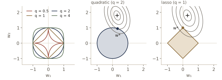
\[\frac{1}{2} \sum_{n=1}^{N} \left\{ t_n - \mathbf{w}^{\mathrm{T}} \boldsymbol{\phi}(\mathbf{x}_n) \right\}^2 + \frac{\lambda}{2} \sum_{j} \lvert w_j \rvert^q .\]The case \(q = 2\) is ridge. The case \(q = 1\) is the lasso (Tibshirani, 1996), whose striking property is sparsity: for large enough \(\lambda\), some weights become exactly zero, and the corresponding basis functions drop out of the model.
The reason is easiest to see through a constrained version of the problem. Using a Lagrange multiplier (Bishop’s Appendix E), minimizing the penalized error for some \(\lambda\) is equivalent to minimizing the plain error \(E_D(\mathbf{w})\) subject to \(\sum_j \lvert w_j \rvert^q \le \eta\) for a matching budget \(\eta\). The constrained optimum is where the smallest elliptical contour of \(E_D\) first touches the constraint region. For \(q = 2\) the region is a disk, whose boundary is smooth, so the touching point is generically off the axes. For \(q = 1\) the region is a diamond with corners on the axes, and an ellipse coming from a generic direction is quite likely to touch a corner first, where one coordinate is exactly zero. For \(q < 1\) the region is even more pointed (and no longer convex).
The lasso error is not differentiable where a weight is zero, so there is no closed form. Coordinate descent is a simple and effective solver: cycle through the weights, and minimize over one weight at a time with the others held fixed. Fix every weight except \(w_j\) and let \(\mathbf{r}_j = \mathbf{t} - \sum_{k \ne j} w_k \boldsymbol{\varphi}_k\) be the partial residual. The error as a function of \(w_j\) alone is
\[\frac{1}{2} \lVert \mathbf{r}_j - w_j \boldsymbol{\varphi}_j \rVert^2 + \frac{\lambda}{2} \lvert w_j \rvert + \text{const},\]a one-dimensional parabola plus a kink at zero. Write \(\rho_j = \boldsymbol{\varphi}_j^{\mathrm{T}} \mathbf{r}_j\) and \(z_j = \lVert \boldsymbol{\varphi}_j \rVert^2\). For \(w_j > 0\) the derivative is \(z_j w_j - \rho_j + \lambda/2\), which vanishes at \(w_j = (\rho_j - \lambda/2)/z_j\), valid only if \(\rho_j > \lambda/2\); the case \(w_j < 0\) is symmetric; and if \(\lvert \rho_j \rvert \le \lambda/2\) neither side has a stationary point and the minimum sits at the kink, \(w_j = 0\). All three cases are one formula, the soft-thresholding operator:
\[w_j = \frac{\operatorname{sign}(\rho_j) \max\left(\lvert \rho_j \rvert - \lambda/2, \, 0\right)}{z_j} .\]Unlike ridge, which shrinks every weight by a factor, soft thresholding subtracts a fixed amount and clips at zero: small correlations with the residual produce exactly zero weights.
How do we know the answer is right? A convex function is minimized where zero belongs to its subgradient. For the lasso that gives the optimality (Karush–Kuhn–Tucker) conditions: with \(\mathbf{g} = \mathbf{\Phi}^{\mathrm{T}} (\mathbf{t} - \mathbf{\Phi} \mathbf{w})\), every nonzero weight must satisfy \(g_j = \frac{\lambda}{2} \operatorname{sign}(w_j)\), and every zero weight must satisfy \(\lvert g_j \rvert \le \frac{\lambda}{2}\). The code checks these.
def soft_threshold(rho, c):
    return np.sign(rho) * max(abs(rho) - c, 0.0)

def fit_lasso(Phi, t, lam, max_sweeps=20000, tol=1e-12):
    """Coordinate descent for 1/2 ||t - Phi w||^2 + (lam/2) sum_j |w_j|."""
    M = Phi.shape[1]
    w = np.zeros(M)
    r = t.copy()                       # full residual t - Phi w
    z = np.sum(Phi**2, axis=0)
    for sweep in range(max_sweeps):
        w_old = w.copy()
        for j in range(M):
            r = r + Phi[:, j] * w[j]   # partial residual r_j
            w[j] = soft_threshold(Phi[:, j] @ r, lam / 2) / z[j]
            r = r - Phi[:, j] * w[j]
        if np.max(np.abs(w - w_old)) < tol:
            break
    return w + 0.0, sweep + 1          # + 0.0 turns -0.0 into 0.0

def kkt_violation(Phi, t, w, lam):
    """Largest violation of the lasso optimality conditions (0 at the exact optimum)."""
    g = Phi.T @ (t - Phi @ w)
    nz = w != 0
    v1 = np.abs(g[nz] - lam / 2 * np.sign(w[nz]))
    v2 = np.maximum(np.abs(g[~nz]) - lam / 2, 0)
    return np.max(np.concatenate([v1, v2, [0.0]]))

print(" lambda  sweeps  nonzero  KKT violation   lasso weights")
for lam in [0.01, 0.3, 1.0, 3.0, 10.0]:
    w_l, sweeps = fit_lasso(Phi, t, lam)
    print(f"{lam:7.2f}  {sweeps:6d}  {np.sum(w_l != 0):5d}     {kkt_violation(Phi, t, w_l, lam):.1e}    {w_l}")
w_r = fit_ridge(Phi, t, 3.0)
print(f"ridge, lambda = 3: smallest |w_j| = {np.min(np.abs(w_r)):.4f}, exact zeros: {np.sum(w_r == 0)}")
 lambda  sweeps  nonzero  KKT violation   lasso weights
   0.01    8293      9     2.1e-11    [ 0.2253 -0.1027  0.3717  0.      0.9957 -1.0648  0.5728 -0.7548 -1.1451
  0.5656]
   0.30     975      7     1.8e-11    [ 0.1713  0.      0.0896  0.4895  0.4104 -0.3725  0.     -0.9144 -0.3713
  0.    ]
   1.00      46      4     1.7e-12    [ 0.      0.      0.      0.8415  0.1193  0.      0.     -0.8423 -0.0839
  0.    ]
   3.00      40      3     1.9e-12    [ 0.      0.      0.      0.7191  0.0432  0.      0.     -0.6147  0.
  0.    ]
  10.00       2      1     8.9e-16    [0.     0.     0.     0.1162 0.     0.     0.     0.     0.     0.    ]
ridge, lambda = 3: smallest |w_j| = 0.0204, exact zeros: 0
As \(\lambda\) grows, the lasso switches basis functions off one after another, until at \(\lambda = 10\) a single bump remains. At every \(\lambda\) the optimality conditions hold to rounding error, so coordinate descent has found the true minimum. Ridge with a comparable penalty leaves every weight nonzero. Note also the number of sweeps: at small \(\lambda\), where the lasso is nearly plain least squares on our badly conditioned basis, coordinate descent needs thousands of passes, for the same reason LMS was slow.
Watch out. Sparsity makes the lasso attractive for choosing a few relevant features, but the selection it makes is not stable when features are strongly correlated: among a group of nearly interchangeable basis functions, it tends to keep one and drop the others, and which one it keeps can flip with a small change in the data. Our overlapping Gaussian bumps are exactly such a group.
Regularization lets a flexible model be trained on a small data set without severe overfitting, by limiting its effective complexity. For the rest of the module we stay with the quadratic regularizer, because it keeps everything in closed form and, as we will see, has a clean Bayesian meaning.
Multiple outputs
Sometimes we predict \(K > 1\) targets at once, collected in a vector \(\mathbf{t}\). One option is a separate model, with its own basis functions, for each target. The common choice is to share one set of basis functions and give each target its own weights:
\[\mathbf{y}(\mathbf{x}, \mathbf{W}) = \mathbf{W}^{\mathrm{T}} \boldsymbol{\phi}(\mathbf{x}),\]where \(\mathbf{W}\) is an \(M \times K\) matrix whose column \(k\) holds the weights for target \(k\). With isotropic Gaussian noise, \(p(\mathbf{t} \mid \mathbf{x}, \mathbf{W}, \beta) = \mathcal{N}(\mathbf{t} \mid \mathbf{W}^{\mathrm{T}} \boldsymbol{\phi}(\mathbf{x}), \beta^{-1} \mathbf{I})\), stack the target vectors as the rows of an \(N \times K\) matrix \(\mathbf{T}\). The log likelihood is \(\frac{NK}{2} \ln \frac{\beta}{2\pi} - \frac{\beta}{2} \sum_n \lVert \mathbf{t}_n - \mathbf{W}^{\mathrm{T}} \boldsymbol{\phi}(\mathbf{x}_n) \rVert^2\), and the squared norm is a sum over the \(K\) components, each involving only its own column of \(\mathbf{W}\). So the problem splits into \(K\) independent least-squares problems,
\[\mathbf{W}_{\mathrm{ML}} = \left(\mathbf{\Phi}^{\mathrm{T}} \mathbf{\Phi}\right)^{-1} \mathbf{\Phi}^{\mathrm{T}} \mathbf{T} = \mathbf{\Phi}^{\dagger} \mathbf{T},\]which share the one pseudo-inverse \(\mathbf{\Phi}^{\dagger}\). The same decoupling holds for a general noise covariance (Bishop Exercise 3.6), because the weights only set the mean, and the maximum likelihood mean of a Gaussian does not depend on its covariance.
t2 = np.cos(2 * np.pi * x) + np.random.default_rng(2).normal(0, NOISE_SD, len(x))
T = np.column_stack([t, t2])                 # N x K targets, K = 2
W = fit_ml(Phi, T)                           # one call fits both columns
print("W shape:", W.shape)
print(f"max difference from two separate fits: "
      f"{max(np.max(np.abs(W[:, 0] - fit_ml(Phi, t))), np.max(np.abs(W[:, 1] - fit_ml(Phi, t2)))):.1e}")
W shape: (10, 2)
max difference from two separate fits: 3.6e-15
From here on we return to a single target.
The bias–variance decomposition
Regularization shifts the question of complexity to the choice of \(\lambda\). Before the Bayesian answer, we look at the frequentist view, which splits the expected error of a learning method into pieces that react in opposite ways to model flexibility.
Deriving the decomposition
Under squared loss the best possible predictor is the regression function \(h(\mathbf{x}) = \mathbb{E}[t \mid \mathbf{x}] = \int t \, p(t \mid \mathbf{x}) \, dt\). In module 01 we showed that the expected loss of any predictor \(y(\mathbf{x})\) splits as
\[\mathbb{E}[L] = \int \{ y(\mathbf{x}) - h(\mathbf{x}) \}^2 p(\mathbf{x}) \, d\mathbf{x} + \iint \{ h(\mathbf{x}) - t \}^2 p(\mathbf{x}, t) \, d\mathbf{x} \, dt .\]The second term is the noise in the data: no predictor can remove it. The first term is where learning succeeds or fails. (Keep separate two uses of “squared error”: the squared loss here judges predictions, while the sum-of-squares error \(E_D\) was a fitting criterion. We could fit by any method, Bayesian or regularized, and still judge the result with squared loss.)
With a finite data set \(\mathcal{D}\) we cannot know \(h\); we get a predictor \(y(\mathbf{x}; \mathcal{D})\) that depends on the particular data we happened to see. The frequentist move is a thought experiment: imagine many independent data sets of the same size \(N\), all drawn from \(p(\mathbf{x}, t)\), run the learning method on each, and average over the ensemble. Write \(\bar{y}(\mathbf{x}) = \mathbb{E}_{\mathcal{D}}[y(\mathbf{x}; \mathcal{D})]\) for the average prediction. At a fixed \(\mathbf{x}\), add and subtract \(\bar{y}\):
\[\begin{aligned} \{ y(\mathbf{x}; \mathcal{D}) - h(\mathbf{x}) \}^2 &= \{ y(\mathbf{x}; \mathcal{D}) - \bar{y}(\mathbf{x}) \}^2 + \{ \bar{y}(\mathbf{x}) - h(\mathbf{x}) \}^2 \\ &\quad + 2 \{ y(\mathbf{x}; \mathcal{D}) - \bar{y}(\mathbf{x}) \} \{ \bar{y}(\mathbf{x}) - h(\mathbf{x}) \} . \end{aligned}\]Now average over \(\mathcal{D}\). The second factor of the cross term does not depend on \(\mathcal{D}\), and the first factor averages to \(\bar{y} - \bar{y} = 0\), so the cross term vanishes:
\[\mathbb{E}_{\mathcal{D}}\left[ \{ y(\mathbf{x}; \mathcal{D}) - h(\mathbf{x}) \}^2 \right] = \underbrace{\{ \bar{y}(\mathbf{x}) - h(\mathbf{x}) \}^2}_{(\text{bias})^2} + \underbrace{\mathbb{E}_{\mathcal{D}}\left[ \{ y(\mathbf{x}; \mathcal{D}) - \bar{y}(\mathbf{x}) \}^2 \right]}_{\text{variance}} .\]The squared bias measures how far the average prediction is from the truth: a systematic error that would persist even with infinitely many data sets to average. The variance measures how much the prediction from one data set scatters around that average: how sensitive the method is to the particular sample. Integrating over \(\mathbf{x}\) with weight \(p(\mathbf{x})\) and putting the pieces together:
Result. For squared loss, averaged over data sets of a fixed size: expected loss = (bias)² + variance + noise.
Here the three terms are
\[\begin{aligned} (\text{bias})^2 &= \int \{ \bar{y}(\mathbf{x}) - h(\mathbf{x}) \}^2 p(\mathbf{x}) \, d\mathbf{x}, \\ \text{variance} &= \int \mathbb{E}_{\mathcal{D}}\left[ \{ y(\mathbf{x}; \mathcal{D}) - \bar{y}(\mathbf{x}) \}^2 \right] p(\mathbf{x}) \, d\mathbf{x}, \\ \text{noise} &= \iint \{ h(\mathbf{x}) - t \}^2 p(\mathbf{x}, t) \, d\mathbf{x} \, dt . \end{aligned}\]A rigid model (few basis functions, or a large \(\lambda\)) gives similar answers on every data set, so low variance, but it may be unable to follow \(h\), so high bias. A flexible model can follow \(h\) on average, low bias, but fits each data set’s noise, high variance. The best predictor balances the two.
An experiment with many data sets
We can run the thought experiment for real. We draw \(L = 100\) data sets of \(N = 25\) points from the sine curve, fit each with a flexible model (24 Gaussian bumps of width 0.05 plus a bias, so \(M = 25\), as many parameters as data points) by ridge regression, and repeat for a range of \(\lambda\). With the fits \(y^{(l)}(x)\), \(l = 1, \dots, L\), the integrals become averages: the average prediction is \(\bar{y}(x) = \frac{1}{L} \sum_l y^{(l)}(x)\), and we approximate the integrals over \(x\) by averages over 1000 test inputs drawn from \(p(x)\),
\[\begin{aligned} (\text{bias})^2 &\approx \frac{1}{N_{\text{test}}} \sum_{i} \{ \bar{y}(x_i) - h(x_i) \}^2, \\ \text{variance} &\approx \frac{1}{N_{\text{test}}} \sum_{i} \frac{1}{L} \sum_{l} \{ y^{(l)}(x_i) - \bar{y}(x_i) \}^2 . \end{aligned}\]We also measure the actual test error, the squared difference between predictions and noisy test targets, averaged over test points and data sets.
MU24, S24 = np.linspace(0, 1, 24), 0.05

def bias_variance(ln_lams, L=100, N=25, n_test=1000, seed=7):
    """Ridge fits to L data sets; returns bias^2, variance, and test error for each ln(lambda)."""
    g = np.random.default_rng(seed)
    X = g.uniform(0, 1, (L, N))
    Tr = np.sin(2 * np.pi * X) + g.normal(0, NOISE_SD, (L, N))
    x_te = g.uniform(0, 1, n_test)
    t_te = np.sin(2 * np.pi * x_te) + g.normal(0, NOISE_SD, n_test)
    h = np.sin(2 * np.pi * x_te)                          # the regression function
    Phi_te = design_matrix(x_te, gauss_basis, MU24, S24)
    Phis = [design_matrix(X[l], gauss_basis, MU24, S24) for l in range(L)]
    rows = []
    for ln_lam in ln_lams:
        Y = np.array([Phi_te @ fit_ridge(Phis[l], Tr[l], np.exp(ln_lam)) for l in range(L)])
        ybar = Y.mean(axis=0)
        bias2 = np.mean((ybar - h) ** 2)
        var = np.mean(np.mean((Y - ybar) ** 2, axis=0))
        test = np.mean((Y - t_te) ** 2)
        pointwise = np.mean((Y - h) ** 2, axis=0)         # E_D[(y - h)^2] at each x
        gap = np.max(np.abs(pointwise - ((ybar - h) ** 2 + np.mean((Y - ybar) ** 2, axis=0))))
        rows.append((ln_lam, bias2, var, test, gap))
    return np.array(rows)

ln_lams = np.arange(-6, 3.01, 0.25)
bv = bias_variance(ln_lams)
print(" ln lambda   bias^2   variance    sum    test error")
for ln_lam, b2, v, te, _ in bv[::4]:
    print(f"{ln_lam:9.2f}   {b2:.4f}    {v:.4f}   {b2 + v:.4f}    {te:.4f}")
best = bv[np.argmin(bv[:, 1] + bv[:, 2])]
print(f"minimum of bias^2 + variance at ln lambda = {best[0]:.2f}; "
      f"minimum test error at ln lambda = {bv[np.argmin(bv[:, 3]), 0]:.2f}")
print(f"test error - (bias^2 + variance) at the minimum: {best[3] - best[1] - best[2]:.4f}  "
      f"(noise variance {NOISE_SD**2:.2f})")
print(f"largest pointwise gap in the decomposition: {np.max(bv[:, 4]):.1e}")
 ln lambda   bias^2   variance    sum    test error
    -6.00   0.0065    0.3292   0.3357    0.4219
    -5.00   0.0031    0.1910   0.1941    0.2803
    -4.00   0.0017    0.1227   0.1243    0.2103
    -3.00   0.0012    0.0834   0.0845    0.1704
    -2.00   0.0014    0.0583   0.0597    0.1454
    -1.00   0.0034    0.0419   0.0452    0.1308
     0.00   0.0119    0.0306   0.0426    0.1282
     1.00   0.0437    0.0228   0.0664    0.1522
     2.00   0.1282    0.0164   0.1446    0.2306
     3.00   0.2628    0.0096   0.2724    0.3586
minimum of bias^2 + variance at ln lambda = -0.25; minimum test error at ln lambda = -0.25
test error - (bias^2 + variance) at the minimum: 0.0856  (noise variance 0.09)
largest pointwise gap in the decomposition: 7.8e-16
The table shows the trade-off. At small \(\lambda\) (the top rows) the squared bias is tiny but the variance is large; at large \(\lambda\) the variance is small but the squared bias dominates. Their sum is smallest at \(\ln \lambda = -0.25\), and the test error is smallest at the same place. The gap between the test error and bias² + variance is close to 0.09, the noise variance \(0.3^2\), as the decomposition predicts, and the pointwise identity holds to rounding error (it is an algebraic identity for the empirical averages too).
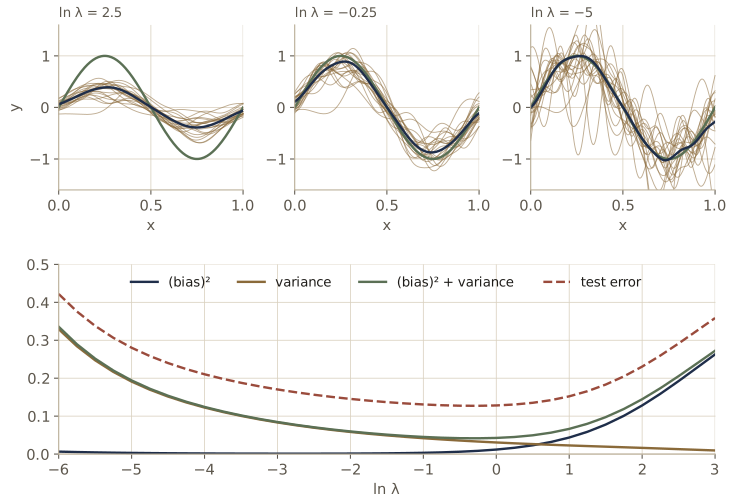
Look at the top-right panel: individually, the lightly regularized fits are wild, yet their average is almost exactly the sine curve. Averaging many flexible fits removes variance while keeping the low bias. This is a first hint of why Bayesian averaging, over the posterior on the weights rather than over data sets, works so well, and of the committee methods in module 14.
What the decomposition does and does not buy us
The decomposition is a good way to think about model complexity, but it is of limited use for choosing it. It averages over an ensemble of data sets, and in practice we have one. If we did have 100 independent data sets, the sensible thing would be to pool them into one large training set, which would reduce overfitting far more than any choice of \(\lambda\). We need a method that works from the single data set we actually have. Cross-validation (module 01) is one; the Bayesian treatment below is another.
Bayesian linear regression
Maximum likelihood cannot choose the model complexity by itself, because the likelihood always prefers the more flexible model. Held-out data can choose it, but costs data and computation. The Bayesian treatment of linear regression avoids overfitting by averaging over the weights instead of picking one setting, and, as we will see in the last two sections, leads to a way of setting the complexity from the training data alone. For now we treat the noise precision \(\beta\) as known.
The posterior over the weights
The likelihood \(p(\mathbf{t} \mid \mathbf{w}) = \prod_n \mathcal{N}(t_n \mid \mathbf{w}^{\mathrm{T}} \boldsymbol{\phi}(\mathbf{x}_n), \beta^{-1})\) has a logarithm that is a quadratic function of \(\mathbf{w}\). A Gaussian prior is therefore conjugate (module 02): the posterior will be Gaussian as well. Take the prior \(p(\mathbf{w}) = \mathcal{N}(\mathbf{w} \mid \mathbf{m}_0, \mathbf{S}_0)\) and derive the posterior by completing the square. Up to terms that do not involve \(\mathbf{w}\),
\[\begin{aligned} \ln p(\mathbf{w} \mid \mathbf{t}) &= -\frac{\beta}{2} (\mathbf{t} - \mathbf{\Phi} \mathbf{w})^{\mathrm{T}} (\mathbf{t} - \mathbf{\Phi} \mathbf{w}) - \frac{1}{2} (\mathbf{w} - \mathbf{m}_0)^{\mathrm{T}} \mathbf{S}_0^{-1} (\mathbf{w} - \mathbf{m}_0) + \text{const} \\ &= -\frac{1}{2} \mathbf{w}^{\mathrm{T}} \left( \mathbf{S}_0^{-1} + \beta \mathbf{\Phi}^{\mathrm{T}} \mathbf{\Phi} \right) \mathbf{w} + \mathbf{w}^{\mathrm{T}} \left( \mathbf{S}_0^{-1} \mathbf{m}_0 + \beta \mathbf{\Phi}^{\mathrm{T}} \mathbf{t} \right) + \text{const}. \end{aligned}\]The log of a Gaussian \(\mathcal{N}(\mathbf{w} \mid \mathbf{m}_N, \mathbf{S}_N)\) is \(-\frac{1}{2} \mathbf{w}^{\mathrm{T}} \mathbf{S}_N^{-1} \mathbf{w} + \mathbf{w}^{\mathrm{T}} \mathbf{S}_N^{-1} \mathbf{m}_N + \text{const}\). Matching the quadratic term and then the linear term:
Result. With prior \(\mathcal{N}(\mathbf{w} \mid \mathbf{m}_0, \mathbf{S}_0)\) and Gaussian noise of precision \(\beta\), the posterior is \(p(\mathbf{w} \mid \mathbf{t}) = \mathcal{N}(\mathbf{w} \mid \mathbf{m}_N, \mathbf{S}_N)\) with \(\mathbf{S}_N^{-1} = \mathbf{S}_0^{-1} + \beta \mathbf{\Phi}^{\mathrm{T}} \mathbf{\Phi}\) and \(\mathbf{m}_N = \mathbf{S}_N \left( \mathbf{S}_0^{-1} \mathbf{m}_0 + \beta \mathbf{\Phi}^{\mathrm{T}} \mathbf{t} \right)\).
Read it as “precisions add”: the posterior precision is the prior precision plus the precision contributed by the data. Some consequences:
- A Gaussian’s mode is its mean, so the most probable weights are \(\mathbf{w}_{\mathrm{MAP}} = \mathbf{m}_N\).
- With no data (\(N = 0\)) the posterior is the prior. With a very broad prior, \(\mathbf{S}_0 = \alpha^{-1} \mathbf{I}\) and \(\alpha \to 0\), the mean tends to \(\mathbf{w}_{\mathrm{ML}}\).
- The result is sequential for free. The posterior after some data is a Gaussian, so it can serve as the prior for the next batch, and the formula applies again. Because precisions and the terms \(\beta \boldsymbol{\phi}_n t_n\) simply accumulate, processing the data one point at a time gives exactly the same posterior as processing them all at once.
From now on we use the simplest prior, a zero-mean isotropic Gaussian with a single precision hyperparameter \(\alpha\) (a parameter of the prior rather than of the model):
\[p(\mathbf{w} \mid \alpha) = \mathcal{N}(\mathbf{w} \mid \mathbf{0}, \alpha^{-1} \mathbf{I}), \qquad \mathbf{S}_N^{-1} = \alpha \mathbf{I} + \beta \mathbf{\Phi}^{\mathrm{T}} \mathbf{\Phi}, \qquad \mathbf{m}_N = \beta \mathbf{S}_N \mathbf{\Phi}^{\mathrm{T}} \mathbf{t} .\]The log posterior is then \(-\frac{\beta}{2} \sum_n \{ t_n - \mathbf{w}^{\mathrm{T}} \boldsymbol{\phi}(\mathbf{x}_n) \}^2 - \frac{\alpha}{2} \mathbf{w}^{\mathrm{T}} \mathbf{w} + \text{const}\). Divide by \(\beta\) and flip the sign: maximizing the posterior is ridge regression with \(\lambda = \alpha / \beta\). The ridge penalty is a Gaussian prior in disguise, and the regularization coefficient is the ratio of the prior precision to the noise precision.
def posterior(Phi, t, alpha, beta):
    """m_N and S_N for the prior N(0, alpha^-1 I) (Bishop eqs. 3.53-3.54), via Cholesky."""
    M = Phi.shape[1]
    A = alpha * np.eye(M) + beta * Phi.T @ Phi         # S_N^{-1}
    c = cho_factor(A)
    m_N = beta * cho_solve(c, Phi.T @ t)
    S_N = cho_solve(c, np.eye(M))
    return m_N, S_N

alpha = 2.0
m_N, S_N = posterior(Phi, t, alpha, BETA_TRUE)
w_ridge = fit_ridge(Phi, t, alpha / BETA_TRUE)
print(f"MAP weights vs ridge with lambda = alpha/beta: max difference {np.max(np.abs(m_N - w_ridge)):.1e}")
print("posterior sd of each weight:", np.sqrt(np.diag(S_N)))
MAP weights vs ridge with lambda = alpha/beta: max difference 2.3e-15
posterior sd of each weight: [0.3782 0.4268 0.3889 0.3662 0.3738 0.3967 0.4873 0.3865 0.4731 0.3981]
The posterior mean equals the ridge solution, and the posterior standard deviations tell us how well the data pin down each weight: the prior alone would give \(\alpha^{-1/2} \approx 0.71\), and 25 points have narrowed every weight to between about 0.37 and 0.49. That is not very tight, because the overlapping bumps can partly stand in for one another.
Sequential Bayesian learning of a straight line
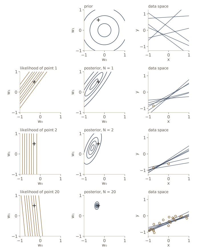
A model with two parameters lets us draw the whole posterior. Take \(y(x, \mathbf{w}) = w_0 + w_1 x\), and generate data from the line \(-0.3 + 0.5 x\) at inputs uniform on \([-1, 1]\), with Gaussian noise of standard deviation 0.2 (the setup of Bishop §3.3.1). We treat the noise as known, \(\beta = 1/0.2^2 = 25\), fix \(\alpha = 2\), and feed the points in one at a time. For the sequential update we keep the posterior in precision form, \((\mathbf{m}, \mathbf{P} = \mathbf{S}^{-1})\), and apply the general result with the current posterior as the prior.
def update(m0, P0, Phi_new, t_new, beta):
    """Posterior (mean, precision) from the prior (m0, P0) after the data (Phi_new, t_new)."""
    P = P0 + beta * Phi_new.T @ Phi_new                  # precisions add
    m = np.linalg.solve(P, P0 @ m0 + beta * Phi_new.T @ t_new)
    return m, P

A_TRUE, LINE_SD, ALPHA_LINE = np.array([-0.3, 0.5]), 0.2, 2.0
BETA_LINE = 1 / LINE_SD**2
g = np.random.default_rng(11)
x_line = g.uniform(-1, 1, 20)
t_line = A_TRUE[0] + A_TRUE[1] * x_line + g.normal(0, LINE_SD, 20)
Phi_line = design_matrix(x_line, lambda x: x[:, None])      # columns 1, x

m, P = np.zeros(2), ALPHA_LINE * np.eye(2)
print("  n   posterior mean       posterior sd       corr(w0, w1)")
for n in range(21):
    if n > 0:
        m, P = update(m, P, Phi_line[n - 1:n], t_line[n - 1:n], BETA_LINE)
    if n in (0, 1, 2, 5, 20):
        S = np.linalg.inv(P)                                  # 2 x 2: fine to invert here
        sd = np.sqrt(np.diag(S))
        print(f"{n:3d}   {m}   {sd}   {S[0, 1] / (sd[0] * sd[1]):+.3f}")

m_batch, S_batch = posterior(Phi_line, t_line, ALPHA_LINE, BETA_LINE)
print(f"sequential vs batch: mean diff {np.max(np.abs(m - m_batch)):.1e}, "
      f"covariance diff {np.max(np.abs(np.linalg.inv(P) - S_batch)):.1e}")
  n   posterior mean       posterior sd       corr(w0, w1)
  0   [0. 0.]   [0.7071 0.7071]   +0.000
  1   [-0.5181  0.3849]   [0.44   0.5753]   +0.899
  2   [-0.5886  0.3021]   [0.1823 0.3308]   +0.649
  5   [-0.4299  0.6062]   [0.1205 0.1894]   +0.677
 20   [-0.3707  0.5   ]   [0.0449 0.0777]   +0.104
sequential vs batch: mean diff 3.9e-16, covariance diff 1.6e-19
Before any data, the posterior is the prior: centered at zero, standard deviation \(1/\sqrt{2} \approx 0.71\) in each direction. One point already moves the mean and makes \(w_0\) and \(w_1\) strongly correlated: a single point says the line passes near it, which constrains a combination of intercept and slope but not each separately. After two points the posterior is compact, and after twenty it is tight around the true values \((-0.3, 0.5)\). The sequential and batch posteriors agree to rounding error.
A Gaussian is not the only possible prior. A family that generalizes it is \(p(\mathbf{w} \mid \alpha) \propto \exp\left(-\frac{\alpha}{2} \sum_j \lvert w_j \rvert^q\right)\), whose most probable weights minimize the \(q\)-norm penalized error from the lasso section; \(q = 1\) gives the lasso as a MAP estimate. Only \(q = 2\) is conjugate to the Gaussian likelihood, though, and for \(q \ne 2\) the posterior mode and mean no longer coincide, so the lasso’s zeros are a property of the MAP point, not of the posterior as a whole.
The predictive distribution
We rarely care about \(\mathbf{w}\) for its own sake; we want to predict \(t\) at a new input \(\mathbf{x}\). The Bayesian predictive distribution averages the noise model over the posterior,
\[p(t \mid \mathbf{x}, \mathbf{t}, \alpha, \beta) = \int p(t \mid \mathbf{x}, \mathbf{w}, \beta) \, p(\mathbf{w} \mid \mathbf{t}, \alpha, \beta) \, d\mathbf{w} .\]There is a short derivation. Under the posterior, \(\mathbf{w} \sim \mathcal{N}(\mathbf{m}_N, \mathbf{S}_N)\), and a new target is \(t = \boldsymbol{\phi}(\mathbf{x})^{\mathrm{T}} \mathbf{w} + \epsilon\) with independent noise \(\epsilon \sim \mathcal{N}(0, \beta^{-1})\). A linear function of a Gaussian vector is Gaussian, with mean \(\boldsymbol{\phi}^{\mathrm{T}} \mathbf{m}_N\) and variance \(\boldsymbol{\phi}^{\mathrm{T}} \mathbf{S}_N \boldsymbol{\phi}\); adding an independent Gaussian adds the means and the variances. (This is the linear-Gaussian marginal of module 02.) So
Result. The predictive distribution is \(p(t \mid \mathbf{x}, \mathbf{t}, \alpha, \beta) = \mathcal{N}\left(t \mid \mathbf{m}_N^{\mathrm{T}} \boldsymbol{\phi}(\mathbf{x}), \, \sigma_N^2(\mathbf{x})\right)\) with \(\sigma_N^2(\mathbf{x}) = \frac{1}{\beta} + \boldsymbol{\phi}(\mathbf{x})^{\mathrm{T}} \mathbf{S}_N \boldsymbol{\phi}(\mathbf{x})\).
The variance has two parts: the noise on the targets, \(1/\beta\), which no amount of data removes, and the uncertainty in the weights, \(\boldsymbol{\phi}^{\mathrm{T}} \mathbf{S}_N \boldsymbol{\phi}\), which shrinks as data accumulate. Each new point adds a positive semidefinite term to \(\mathbf{S}_N^{-1}\), so \(\mathbf{S}_N\) can only shrink, and one can show that \(\sigma_{N+1}^2(\mathbf{x}) \le \sigma_N^2(\mathbf{x})\) at every \(\mathbf{x}\). As \(N \to \infty\) the second term goes to zero and only the noise remains.
We apply this to the running data set with the 9 Gaussian bumps, \(\alpha = 2\) and the true \(\beta\), using the first 1, 2, 4, and all 25 points. The first check compares the formula with brute-force Monte Carlo: sample weights from the posterior, add noise, and look at the spread of the simulated targets.
def predictive(Phi_new, m_N, S_N, beta):
    """Mean and variance of the predictive distribution at the rows of Phi_new (eq. 3.59)."""
    mean = Phi_new @ m_N
    var = 1 / beta + np.sum((Phi_new @ S_N) * Phi_new, axis=1)
    return mean, var

m25, S25 = posterior(Phi, t, alpha, BETA_TRUE)
phi_star = design_matrix(np.array([0.3]), gauss_basis, MU9, S9)
mu_star, var_star = predictive(phi_star, m25, S25, BETA_TRUE)
W_s = rng.multivariate_normal(m25, S25, size=200_000)
t_s = W_s @ phi_star[0] + rng.normal(0, 1 / np.sqrt(BETA_TRUE), len(W_s))
print(f"x = 0.3: formula mean {mu_star[0]:.4f}, sd {np.sqrt(var_star[0]):.4f};  "
      f"Monte Carlo mean {t_s.mean():.4f}, sd {t_s.std():.4f}")

xs = np.linspace(0, 1, 201)
Phi_s = design_matrix(xs, gauss_basis, MU9, S9)
prev = None
for n in [1, 2, 4, 25]:
    mn, Sn = posterior(Phi[:n], t[:n], alpha, BETA_TRUE)
    mean, var = predictive(Phi_s, mn, Sn, BETA_TRUE)
    shrinks = "" if prev is None else f"   sd never larger than before: {np.all(var <= prev + 1e-12)}"
    print(f"N = {n:2d}: predictive sd from {np.sqrt(var.min()):.3f} to {np.sqrt(var.max()):.3f}{shrinks}")
    prev = var
far = design_matrix(np.array([1.6, 3.0, 10.0]), gauss_basis, MU9, S9)
print("x = 1.6, 3, 10 (outside the bumps): sd", np.sqrt(predictive(far, m25, S25, BETA_TRUE)[1]))
print(f"  sqrt(1/beta + var[w0]) = {np.sqrt(1 / BETA_TRUE + S25[0, 0]):.4f}")
m_nb, S_nb = posterior(Phi[:, 1:], t, alpha, BETA_TRUE)          # the same model without the bias
print("  without the bias column: sd", np.sqrt(predictive(far[:, 1:], m_nb, S_nb, BETA_TRUE)[1]))
x = 0.3: formula mean 0.8850, sd 0.3252;  Monte Carlo mean 0.8839, sd 0.3255
N =  1: predictive sd from 0.417 to 1.047
N =  2: predictive sd from 0.415 to 1.006   sd never larger than before: True
N =  4: predictive sd from 0.365 to 0.846   sd never larger than before: True
N = 25: predictive sd from 0.325 to 0.420   sd never larger than before: True
x = 1.6, 3, 10 (outside the bumps): sd [0.4827 0.4827 0.4827]
  sqrt(1/beta + var[w0]) = 0.4827
  without the bias column: sd [0.3 0.3 0.3]
The formula and the simulation agree to about 0.001. The band narrows as data arrive, and it narrows everywhere, never widening, just as the argument above said. With all 25 points its narrowest part is only slightly wider than the noise level 0.3.
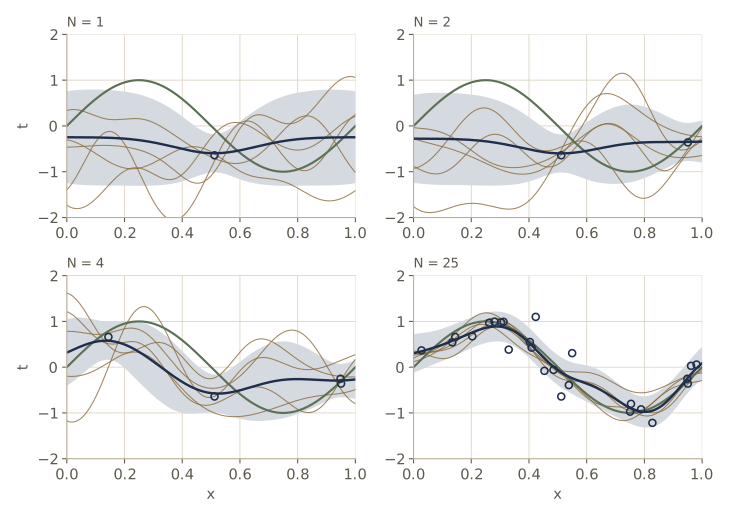
The band shows the uncertainty at each \(x\) separately. The sampled functions show more: they are smooth curves, so if the truth is above the mean at \(x = 0.3\) it is probably also above it at \(x = 0.32\). The predictions at different inputs are correlated through the shared weights, and the next subsection makes that correlation explicit.
Watch out. Look at the last lines of the output. Far from every Gaussian bump, all basis functions except the bias are essentially zero, so the predictive standard deviation settles at \(\sqrt{1/\beta + \operatorname{var}[w_0]}\) and stays there: it is the same at \(x = 10\) as at \(x = 1.6\). Without the bias column it would drop all the way to the noise level 0.3, lower than anywhere inside the data. A model that has never seen anything near \(x = 10\) should be far less sure of itself. Localized fixed bases extrapolate overconfidently; Gaussian processes (module 06) fix this by specifying the covariance of the function directly.
If \(\beta\) is unknown as well, the conjugate prior for \((\mathbf{w}, \beta)\) together is a Gaussian–gamma distribution (module 02), and integrating out \(\beta\) turns the predictive distribution into a Student’s t-distribution, with heavier tails that reflect the extra uncertainty about the noise level (Bishop Exercises 3.12–3.13).
The equivalent kernel
Substitute the posterior mean into the model. The predictive mean at \(\mathbf{x}\) is
\[y(\mathbf{x}, \mathbf{m}_N) = \boldsymbol{\phi}(\mathbf{x})^{\mathrm{T}} \mathbf{m}_N = \beta \boldsymbol{\phi}(\mathbf{x})^{\mathrm{T}} \mathbf{S}_N \mathbf{\Phi}^{\mathrm{T}} \mathbf{t} = \sum_{n=1}^{N} k(\mathbf{x}, \mathbf{x}_n) \, t_n, \qquad k(\mathbf{x}, \mathbf{x}') = \beta \boldsymbol{\phi}(\mathbf{x})^{\mathrm{T}} \mathbf{S}_N \boldsymbol{\phi}(\mathbf{x}') .\]So the prediction is a weighted sum of the training targets. The weight function \(k\) is the equivalent kernel (statisticians also call it the smoother matrix), and a method that predicts by a linear combination of the training targets is a linear smoother. The kernel depends on the training inputs through \(\mathbf{S}_N\), but not on the targets.
Three properties make the kernel worth knowing.
- It is local. For each \(\mathbf{x}\), \(k(\mathbf{x}, \mathbf{x}')\) as a function of \(\mathbf{x}'\) peaks near \(\mathbf{x}\): the prediction leans most on nearby targets. Surprisingly, this holds even for global bases such as polynomials and sigmoids, as the figure below shows.
- Its weights sum to (nearly) one. If every target were 1, a model with a bias would fit them exactly when \(\alpha\) is small and there are more points than basis functions; so \(\sum_n k(\mathbf{x}, \mathbf{x}_n) \approx 1\) at every \(\mathbf{x}\). The weights can be negative, though, so the prediction is not a convex average of the targets.
- It is a covariance. Under the posterior, \(\operatorname{cov}[y(\mathbf{x}), y(\mathbf{x}')] = \boldsymbol{\phi}(\mathbf{x})^{\mathrm{T}} \mathbf{S}_N \boldsymbol{\phi}(\mathbf{x}') = \beta^{-1} k(\mathbf{x}, \mathbf{x}')\), which is the correlation between nearby predictions that the sampled curves showed. And it is an inner product, \(k(\mathbf{x}, \mathbf{z}) = \boldsymbol{\psi}(\mathbf{x})^{\mathrm{T}} \boldsymbol{\psi}(\mathbf{z})\) with \(\boldsymbol{\psi}(\mathbf{x}) = \beta^{1/2} \mathbf{S}_N^{1/2} \boldsymbol{\phi}(\mathbf{x})\), the defining property of the kernels of module 06.
def equivalent_kernel(Phi_query, Phi_train, alpha, beta):
    """k(x, x_n) = beta phi(x)^T S_N phi(x_n) for each query row and training row."""
    _, S_N = posterior(Phi_train, np.zeros(len(Phi_train)), alpha, beta)
    return beta * Phi_query @ S_N @ Phi_train.T

K = equivalent_kernel(Phi_s, Phi, alpha, BETA_TRUE)          # 201 queries x 25 training points
print(f"K t vs m_N^T phi(x): max difference {np.max(np.abs(K @ t - Phi_s @ m25)):.1e}")

# the kernel at x = 0 for three bases, with 200 evenly spaced training inputs on [-1, 1]
x200 = np.linspace(-1, 1, 200)
C9 = np.linspace(-1, 1, 9)
bases = {"polynomial": (poly_basis, 9), "Gaussian": (gauss_basis, C9, 0.2),
         "sigmoidal": (sigmoid_basis, C9, 0.1)}
i0 = np.argmin(np.abs(x200))
print("basis        sum of weights   peak at x'   most negative weight")
for name, (f, *args) in bases.items():
    P200 = design_matrix(x200, f, *args)
    k0 = equivalent_kernel(P200[i0:i0 + 1], P200, 1e-3, BETA_TRUE)[0]
    print(f"{name:11s}   {k0.sum():10.4f}      {x200[np.argmax(k0)]:+.3f}       {k0.min():+.4f}")
K t vs m_N^T phi(x): max difference 4.3e-15
basis        sum of weights   peak at x'   most negative weight
polynomial        1.0000      +0.005       -0.0067
Gaussian          1.0000      +0.005       -0.0112
sigmoidal         1.0000      +0.015       -0.0088
The kernel reproduces the predictive mean exactly. For all three bases the kernel at \(x = 0\) peaks within 0.02 of \(x = 0\) and has weights summing to 1 (with \(\alpha = 10^{-3}\), a nearly flat prior), and all three have some negative weights.
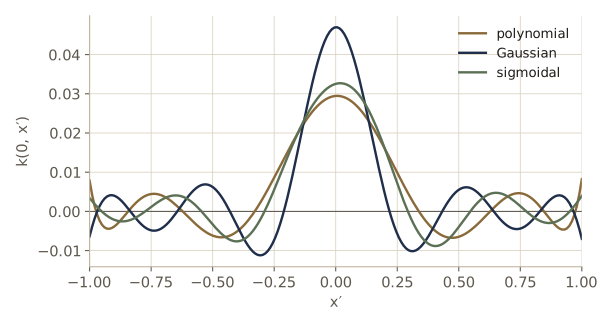
This view suggests a different way to build a regression method: skip the basis functions and write down a localized kernel directly. That idea leads to Gaussian processes in module 06.
Bayesian model comparison
We now turn to choosing between models, from the Bayesian side. The ideas in this section are general; the next section applies them to linear regression.
Evidence, Bayes factors, and model averaging
Suppose we have \(L\) candidate models \(\mathcal{M}_1, \dots, \mathcal{M}_L\). Here a model means a complete probability distribution over the observed data (for regression, over the targets \(\mathbf{t}\) given the inputs), including its priors. We treat our uncertainty about which model generated the data like any other uncertainty, with a prior \(p(\mathcal{M}_i)\) and Bayes’ theorem:
\[p(\mathcal{M}_i \mid \mathcal{D}) \propto p(\mathcal{M}_i) \, p(\mathcal{D} \mid \mathcal{M}_i) .\]With equal prior probabilities, the models are ranked by \(p(\mathcal{D} \mid \mathcal{M}_i)\), the model evidence, also called the marginal likelihood because the parameters have been integrated out:
\[p(\mathcal{D} \mid \mathcal{M}_i) = \int p(\mathcal{D} \mid \mathbf{w}, \mathcal{M}_i) \, p(\mathbf{w} \mid \mathcal{M}_i) \, d\mathbf{w} .\]The ratio \(p(\mathcal{D} \mid \mathcal{M}_i) / p(\mathcal{D} \mid \mathcal{M}_j)\) is the Bayes factor of model \(i\) against model \(j\). Two readings of the evidence help. It is the probability that the model would produce this data set if we first drew parameters from the prior and then drew data from the model: a model is rewarded for having predicted the data before seeing them. And it is the normalizing constant in Bayes’ theorem for the parameters, \(p(\mathbf{w} \mid \mathcal{D}, \mathcal{M}_i) = p(\mathcal{D} \mid \mathbf{w}, \mathcal{M}_i) \, p(\mathbf{w} \mid \mathcal{M}_i) / p(\mathcal{D} \mid \mathcal{M}_i)\).
The fully Bayesian prediction does not pick a model; it averages them, weighting each by its posterior probability:
\[p(t \mid \mathbf{x}, \mathcal{D}) = \sum_{i=1}^{L} p(t \mid \mathbf{x}, \mathcal{M}_i, \mathcal{D}) \, p(\mathcal{M}_i \mid \mathcal{D}) .\]This is a mixture. If two equally probable models predict narrow peaks at two different values, the averaged prediction has two peaks, not one peak in between. Using only the single most probable model is a common approximation called model selection.
Why the evidence prefers simpler models
Why should an integral over parameters penalize complexity? A rough picture helps. Take one parameter \(w\), a flat prior of width \(\Delta w_{\text{prior}}\) (so \(p(w) = 1/\Delta w_{\text{prior}}\)), and suppose the likelihood is sharply peaked at \(w_{\mathrm{MAP}}\) with width \(\Delta w_{\text{posterior}}\). The integral is roughly the height of the peak times its width:
\[p(\mathcal{D}) = \int p(\mathcal{D} \mid w) \, p(w) \, dw \approx p(\mathcal{D} \mid w_{\mathrm{MAP}}) \frac{\Delta w_{\text{posterior}}}{\Delta w_{\text{prior}}}, \qquad \ln p(\mathcal{D}) \approx \ln p(\mathcal{D} \mid w_{\mathrm{MAP}}) + \ln \frac{\Delta w_{\text{posterior}}}{\Delta w_{\text{prior}}} .\]The first term rewards fit. The second, the log of the Occam factor, is negative, because the posterior is narrower than the prior, and it grows in size the more finely the data force us to tune the parameter. With \(M\) parameters, each with a similar ratio, the penalty becomes \(M \ln (\Delta w_{\text{posterior}} / \Delta w_{\text{prior}})\), growing linearly in \(M\). More flexible models fit better but pay a larger Occam penalty, and the evidence peaks at a compromise. (Module 04’s Laplace approximation turns this sketch into a real approximation.)
Another way to see it: think of every possible data set laid out along one axis. Each model spreads a total probability of one over that axis. A simple model can only produce a narrow range of data sets, so it puts high probability on each of them; a very flexible model can produce almost anything, so it spreads its probability thinly. For the data set we actually observed, a model that is too simple assigns it low probability because it cannot produce such data at all, and a model that is too complex assigns it low probability because its probability is spread over too many alternatives. The model of intermediate flexibility wins.
Note. The Occam penalty needs a proper prior. As a Gaussian prior is made broader, \(\Delta w_{\text{prior}}\) grows, and the evidence goes to zero, even though the posterior barely changes. An improper (unnormalizable) prior makes the evidence undefined. Parameter estimation is forgiving about vague priors; model comparison is not.
Computing an evidence
For the linear-Gaussian model the evidence has a closed form, and we can check it against the “sample parameters from the prior” reading. With \(\mathbf{w} \sim \mathcal{N}(\mathbf{0}, \alpha^{-1} \mathbf{I})\) and \(\mathbf{t} = \mathbf{\Phi} \mathbf{w} + \boldsymbol{\epsilon}\), \(\boldsymbol{\epsilon} \sim \mathcal{N}(\mathbf{0}, \beta^{-1} \mathbf{I})\), the targets are a linear function of Gaussians, so (module 02)
\[p(\mathbf{t} \mid \alpha, \beta) = \mathcal{N}\left(\mathbf{t} \mid \mathbf{0}, \, \mathbf{C}\right), \qquad \mathbf{C} = \beta^{-1} \mathbf{I}_N + \alpha^{-1} \mathbf{\Phi} \mathbf{\Phi}^{\mathrm{T}} .\]We compute this for the straight-line data, compare with a Monte Carlo average of the likelihood over prior samples (in log space, with log-sum-exp), show that the evidence falls as the prior is widened, and then run a small model-comparison experiment.
def log_evidence_direct(Phi, t, alpha, beta):
    """ln N(t | 0, beta^-1 I + alpha^-1 Phi Phi^T), via a Cholesky factor of the N x N covariance."""
    N = len(t)
    C = np.eye(N) / beta + Phi @ Phi.T / alpha
    Lc = np.linalg.cholesky(C)
    z = solve_triangular(Lc, t, lower=True)
    return -0.5 * z @ z - np.sum(np.log(np.diag(Lc))) - N / 2 * np.log(2 * np.pi)

def log_likelihood(W, Phi, t, beta):
    """ln p(t | w, beta) for each row w of W."""
    R = t[None, :] - W @ Phi.T
    return len(t) / 2 * np.log(beta / (2 * np.pi)) - beta / 2 * np.sum(R**2, axis=1)

exact = log_evidence_direct(Phi_line, t_line, ALPHA_LINE, BETA_LINE)
W_prior = rng.normal(0, 1 / np.sqrt(ALPHA_LINE), size=(200_000, 2))
mc = logsumexp(log_likelihood(W_prior, Phi_line, t_line, BETA_LINE)) - np.log(len(W_prior))
print(f"line model, 20 points: exact ln evidence {exact:.3f}, Monte Carlo {mc:.3f}")
for a in [2.0, 1e-2, 1e-4, 1e-6]:
    print(f"  alpha = {a:7.0e}  ln evidence = {log_evidence_direct(Phi_line, t_line, a, BETA_LINE):8.3f}")

# data from random lines; compare the line model with a cubic model (both with alpha = 2)
g = np.random.default_rng(21)
wins, lbf = 0, []
for _ in range(500):
    xr = g.uniform(-1, 1, 10)
    wr = g.normal(0, 1 / np.sqrt(ALPHA_LINE), 2)
    tr = wr[0] + wr[1] * xr + g.normal(0, LINE_SD, 10)
    b = (log_evidence_direct(design_matrix(xr, poly_basis, 1), tr, ALPHA_LINE, BETA_LINE)
         - log_evidence_direct(design_matrix(xr, poly_basis, 3), tr, ALPHA_LINE, BETA_LINE))
    lbf.append(b)
    wins += b > 0
print(f"line vs cubic on 500 data sets drawn from the line model: line preferred in {wins},"
      f" mean ln Bayes factor {np.mean(lbf):.3f}")
line model, 20 points: exact ln evidence 1.688, Monte Carlo 1.635
  alpha =   2e+00  ln evidence =    1.688
  alpha =   1e-02  ln evidence =   -3.213
  alpha =   1e-04  ln evidence =   -7.816
  alpha =   1e-06  ln evidence =  -12.421
line vs cubic on 500 data sets drawn from the line model: line preferred in 447, mean ln Bayes factor 0.911
The closed form and the Monte Carlo estimate agree to within about 0.05. Widening the prior drives the evidence down steadily, by about \(\ln 100 \approx 4.6\) for each factor of 100 in \(\alpha\) (each of the two weights contributes \(\frac{1}{2} \ln 100\)), although the posterior mean hardly moves: the Occam factor at work. In the comparison, the cubic model contains the line model as a special case and can always fit at least as well; yet the evidence prefers the true, simpler model on most data sets, and on average (a positive mean log Bayes factor), although not on every single one.
That last observation holds in general. If the data really come from \(\mathcal{M}_1\), the expected log Bayes factor, averaged over data sets drawn from \(\mathcal{M}_1\), is \(\int p(\mathcal{D} \mid \mathcal{M}_1) \ln \frac{p(\mathcal{D} \mid \mathcal{M}_1)}{p(\mathcal{D} \mid \mathcal{M}_2)} \, d\mathcal{D}\), a Kullback–Leibler divergence, which is never negative (module 01). On average, Bayesian model comparison favors the correct model; for a particular finite data set, it can be fooled.
Caveats
The argument assumes the true data-generating process is among the models being compared, which in practice it rarely is. The evidence can also be sensitive to aspects of the prior that hardly affect predictions, such as the tails, or the width of a vague prior, as the \(\alpha\) sweep above showed. So in a real application it is still wise to keep an independent test set to check the final system.
The evidence approximation
A fully Bayesian treatment would put priors on the hyperparameters \(\alpha\) and \(\beta\) too, and integrate them out along with \(\mathbf{w}\):
\[p(t \mid \mathbf{t}) = \iiint p(t \mid \mathbf{w}, \beta) \, p(\mathbf{w} \mid \mathbf{t}, \alpha, \beta) \, p(\alpha, \beta \mid \mathbf{t}) \, d\mathbf{w} \, d\alpha \, d\beta .\]We can integrate over \(\mathbf{w}\) analytically, or over the hyperparameters, but not over all of them at once. The evidence approximation assumes that \(p(\alpha, \beta \mid \mathbf{t})\) is sharply peaked at some \((\hat{\alpha}, \hat{\beta})\), and replaces the integral over the hyperparameters by their values at the peak:
\[p(t \mid \mathbf{t}) \approx p(t \mid \mathbf{t}, \hat{\alpha}, \hat{\beta}) = \int p(t \mid \mathbf{w}, \hat{\beta}) \, p(\mathbf{w} \mid \mathbf{t}, \hat{\alpha}, \hat{\beta}) \, d\mathbf{w} .\]Since \(p(\alpha, \beta \mid \mathbf{t}) \propto p(\mathbf{t} \mid \alpha, \beta) \, p(\alpha, \beta)\), with a fairly flat hyperprior the peak is where the marginal likelihood \(p(\mathbf{t} \mid \alpha, \beta)\) is largest. So we choose the hyperparameters by maximizing the evidence. Statisticians call this empirical Bayes or type-II maximum likelihood; in machine learning it is the evidence approximation. It is maximum likelihood again, but one level up, after the weights have been integrated out, and that makes all the difference: it no longer rewards overfitting.
Evaluating the evidence function
We already have the evidence as an \(N\)-dimensional Gaussian density, but a form in terms of \(M\)-dimensional quantities is cheaper when \(N > M\) and more revealing. Start from the integral over \(\mathbf{w}\) of likelihood times prior:
\[p(\mathbf{t} \mid \alpha, \beta) = \left( \frac{\beta}{2\pi} \right)^{N/2} \left( \frac{\alpha}{2\pi} \right)^{M/2} \int \exp\{ -E(\mathbf{w}) \} \, d\mathbf{w}, \qquad E(\mathbf{w}) = \frac{\beta}{2} \lVert \mathbf{t} - \mathbf{\Phi} \mathbf{w} \rVert^2 + \frac{\alpha}{2} \mathbf{w}^{\mathrm{T}} \mathbf{w} .\]Here \(E(\mathbf{w})\) is \(\beta\) times the ridge error with \(\lambda = \alpha / \beta\). It is quadratic in \(\mathbf{w}\), with Hessian (matrix of second derivatives)
\[\mathbf{A} = \nabla \nabla E(\mathbf{w}) = \alpha \mathbf{I} + \beta \mathbf{\Phi}^{\mathrm{T}} \mathbf{\Phi} = \mathbf{S}_N^{-1},\]and its minimum is at \(\mathbf{m}_N = \beta \mathbf{A}^{-1} \mathbf{\Phi}^{\mathrm{T}} \mathbf{t}\), the posterior mean. A quadratic equals its minimum value plus the Hessian term, exactly:
\[E(\mathbf{w}) = E(\mathbf{m}_N) + \frac{1}{2} (\mathbf{w} - \mathbf{m}_N)^{\mathrm{T}} \mathbf{A} (\mathbf{w} - \mathbf{m}_N), \qquad E(\mathbf{m}_N) = \frac{\beta}{2} \lVert \mathbf{t} - \mathbf{\Phi} \mathbf{m}_N \rVert^2 + \frac{\alpha}{2} \mathbf{m}_N^{\mathrm{T}} \mathbf{m}_N .\]The integral of the Gaussian-shaped factor is its normalizing constant, \(\int \exp\{ -\frac{1}{2} (\mathbf{w} - \mathbf{m}_N)^{\mathrm{T}} \mathbf{A} (\mathbf{w} - \mathbf{m}_N) \} \, d\mathbf{w} = (2\pi)^{M/2} \lvert \mathbf{A} \rvert^{-1/2}\). Collecting terms and taking the log:
Result. The log evidence of the linear basis function model is \(\ln p(\mathbf{t} \mid \alpha, \beta) = \frac{M}{2} \ln \alpha + \frac{N}{2} \ln \beta - E(\mathbf{m}_N) - \frac{1}{2} \ln \lvert \mathbf{A} \rvert - \frac{N}{2} \ln (2\pi)\).
The terms line up with the Occam picture: \(-E(\mathbf{m}_N)\) rewards the fit, and \(\frac{M}{2} \ln \alpha - \frac{1}{2} \ln \lvert \mathbf{A} \rvert = -\frac{1}{2} \ln \lvert \mathbf{A} / \alpha \rvert\) is the log ratio of the posterior volume to the prior volume. We compute \(\ln \lvert \mathbf{A} \rvert\) from the Cholesky factor, as twice the sum of the logs of its diagonal.
def log_evidence(Phi, t, alpha, beta):
    """ln p(t | alpha, beta) from the M x M form (Bishop eq. 3.86); also returns m_N."""
    N, M = Phi.shape
    A = alpha * np.eye(M) + beta * Phi.T @ Phi
    c = cho_factor(A, lower=True)
    m_N = beta * cho_solve(c, Phi.T @ t)
    E_mN = beta / 2 * np.sum((t - Phi @ m_N) ** 2) + alpha / 2 * m_N @ m_N
    logdet_A = 2 * np.sum(np.log(np.diag(c[0])))
    return M / 2 * np.log(alpha) + N / 2 * np.log(beta) - E_mN - logdet_A / 2 - N / 2 * np.log(2 * np.pi), m_N

for a in [0.01, 2.0, 100.0]:
    le, _ = log_evidence(Phi, t, a, BETA_TRUE)
    print(f"alpha = {a:6.2f}:  M x M form {le:9.4f}   N x N Gaussian {log_evidence_direct(Phi, t, a, BETA_TRUE):9.4f}")
alpha =   0.01:  M x M form  -33.6277   N x N Gaussian  -33.6277
alpha =   2.00:  M x M form  -14.2820   N x N Gaussian  -14.2820
alpha = 100.00:  M x M form  -33.2098   N x N Gaussian  -33.2098
The two formulas agree, one working with \(10 \times 10\) matrices and the other with \(25 \times 25\).
Evidence for polynomials of increasing order
Now the example that motivates the whole machinery: which polynomial order does the evidence prefer for a small sine data set? We draw \(N = 10\) points, fix \(\alpha = 5 \times 10^{-3}\) (a broad prior) and the true \(\beta\), and compute the log evidence of polynomials of order \(0, 1, \dots, 9\). As in module 01, “order \(M\)” here means the polynomial \(w_0 + w_1 x + \dots + w_M x^M\), with \(M + 1\) weights. For comparison we also report the root-mean-square (RMS) error of the posterior mean on the training data and on 1000 fresh test points.
x10, t10 = sin_data(10, seed=8)
x_te, t_te = sin_data(1000, seed=99)          # a test set used for the rest of the module
ALPHA_POLY = 5e-3
print("order   ln evidence   train RMS   test RMS")
ev_poly = []
for order in range(10):
    P_tr = design_matrix(x10, poly_basis, order)
    le, m = log_evidence(P_tr, t10, ALPHA_POLY, BETA_TRUE)
    rms_tr = np.sqrt(np.mean((P_tr @ m - t10) ** 2))
    rms_te = np.sqrt(np.mean((design_matrix(x_te, poly_basis, order) @ m - t_te) ** 2))
    ev_poly.append(le)
    print(f"{order:5d}   {le:10.3f}    {rms_tr:8.3f}   {rms_te:8.3f}")
print(f"largest evidence at order {int(np.argmax(ev_poly))}")
order   ln evidence   train RMS   test RMS
    0      -28.734       0.692      0.850
    1      -17.550       0.459      0.627
    2      -19.206       0.447      0.642
    3      -15.327       0.267      0.420
    4      -14.446       0.242      0.388
    5      -14.911       0.249      0.396
    6      -15.458       0.251      0.398
    7      -15.897       0.248      0.392
    8      -16.260       0.245      0.384
    9      -16.586       0.244      0.378
largest evidence at order 4
Read the evidence column from the top. Order 0 (a constant) fits badly and has low evidence. Order 1 fits much better, and the evidence jumps. Order 2 barely improves the fit, because the sine curve on \([0, 1]\) is antisymmetric about \(x = 0.5\) and gains little from a quadratic term, so the extra parameter’s Occam penalty wins and the evidence drops. Order 3 improves the fit a lot, order 4 a little more, and the evidence peaks at order 4. Beyond that, the training error keeps creeping down, but the evidence declines steadily, because each extra parameter must be paid for. The test error, meanwhile, is nearly flat from order 4 on (it is even slightly lowest at order 9, because the prior keeps the high-order fits tame), so it would hardly help us choose. The evidence picks the simplest model that explains the data well, using the training data alone.
Maximizing the evidence
Now let the data choose \(\alpha\) and \(\beta\) directly by maximizing the log evidence. The awkward term is \(\ln \lvert \mathbf{A} \rvert\), and eigenvalues make it easy. Let
\[\left( \beta \mathbf{\Phi}^{\mathrm{T}} \mathbf{\Phi} \right) \mathbf{u}_i = \lambda_i \mathbf{u}_i, \qquad i = 1, \dots, M .\](These \(\lambda_i\) are eigenvalues, unrelated to the regularization coefficient.) Then \(\mathbf{A} = \alpha \mathbf{I} + \beta \mathbf{\Phi}^{\mathrm{T}} \mathbf{\Phi}\) has eigenvalues \(\alpha + \lambda_i\), so \(\ln \lvert \mathbf{A} \rvert = \sum_i \ln (\alpha + \lambda_i)\) and
\[\frac{\partial}{\partial \alpha} \ln \lvert \mathbf{A} \rvert = \sum_{i} \frac{1}{\lambda_i + \alpha} .\]What about \(E(\mathbf{m}_N)\), which depends on \(\alpha\) both directly and through \(\mathbf{m}_N\)? Because \(\mathbf{m}_N\) minimizes \(E\), the gradient of \(E\) with respect to \(\mathbf{w}\) vanishes there, so a small change in \(\mathbf{m}_N\) does not change \(E(\mathbf{m}_N)\) to first order. Only the explicit dependence counts: \(\partial E(\mathbf{m}_N) / \partial \alpha = \frac{1}{2} \mathbf{m}_N^{\mathrm{T}} \mathbf{m}_N\). Setting the derivative of the log evidence to zero,
\[0 = \frac{M}{2\alpha} - \frac{1}{2} \mathbf{m}_N^{\mathrm{T}} \mathbf{m}_N - \frac{1}{2} \sum_i \frac{1}{\lambda_i + \alpha} .\]Multiply by \(2\alpha\) and rearrange: \(\alpha \mathbf{m}_N^{\mathrm{T}} \mathbf{m}_N = M - \sum_i \frac{\alpha}{\lambda_i + \alpha} = \sum_i \frac{\lambda_i}{\lambda_i + \alpha}\). Define
\[\gamma = \sum_{i=1}^{M} \frac{\lambda_i}{\alpha + \lambda_i}, \qquad\text{so that}\qquad \alpha = \frac{\gamma}{\mathbf{m}_N^{\mathrm{T}} \mathbf{m}_N} .\]For \(\beta\) the same steps work. The eigenvalues are proportional to \(\beta\), so \(\partial \lambda_i / \partial \beta = \lambda_i / \beta\) and \(\partial \ln \lvert \mathbf{A} \rvert / \partial \beta = \frac{1}{\beta} \sum_i \frac{\lambda_i}{\lambda_i + \alpha} = \gamma / \beta\). The explicit derivative of \(E(\mathbf{m}_N)\) is \(\frac{1}{2} \sum_n \{ t_n - \mathbf{m}_N^{\mathrm{T}} \boldsymbol{\phi}(\mathbf{x}_n) \}^2\). Setting the derivative to zero gives \(0 = \frac{N}{2\beta} - \frac{1}{2} \sum_n \{ t_n - \mathbf{m}_N^{\mathrm{T}} \boldsymbol{\phi}(\mathbf{x}_n) \}^2 - \frac{\gamma}{2\beta}\), that is,
\[\frac{1}{\beta} = \frac{1}{N - \gamma} \sum_{n=1}^{N} \left\{ t_n - \mathbf{m}_N^{\mathrm{T}} \boldsymbol{\phi}(\mathbf{x}_n) \right\}^2 .\]Both equations are implicit: \(\gamma\) and \(\mathbf{m}_N\) depend on \(\alpha\) and \(\beta\). The standard approach is a fixed-point iteration: start from a guess, compute \(\mathbf{m}_N\) and \(\gamma\), re-estimate \(\alpha\) and \(\beta\) from the two formulas, and repeat. The eigenvalues of \(\mathbf{\Phi}^{\mathrm{T}} \mathbf{\Phi}\) are computed once; each iteration only rescales them by the current \(\beta\).
First, to see what the iteration is looking for, fix \(\beta\) at its true value and scan \(\alpha\) on the running data set with the 9-bump model. At the optimum the two sides of \(\alpha \mathbf{m}_N^{\mathrm{T}} \mathbf{m}_N = \gamma\) must meet. Note that \(\alpha \mathbf{m}_N^{\mathrm{T}} \mathbf{m}_N = 2 \alpha E_W(\mathbf{m}_N)\).
eig0 = np.linalg.eigvalsh(Phi.T @ Phi)              # computed once

def gamma_of(alpha, beta):
    lam = beta * eig0
    return np.sum(lam / (alpha + lam))

Phi_te = design_matrix(x_te, gauss_basis, MU9, S9)
ln_alphas = np.linspace(-5, 5, 201)
scan = []
for la in ln_alphas:
    le, m = log_evidence(Phi, t, np.exp(la), BETA_TRUE)
    test_rms = np.sqrt(np.mean((Phi_te @ m - t_te) ** 2))
    scan.append((le, gamma_of(np.exp(la), BETA_TRUE), np.exp(la) * m @ m, test_rms))
scan = np.array(scan)
cross = ln_alphas[np.argmin(np.abs(scan[:, 1] - scan[:, 2]))]
print(f"gamma = 2 alpha E_W at ln alpha = {cross:.2f}")
print(f"largest evidence at ln alpha = {ln_alphas[np.argmax(scan[:, 0])]:.2f}")
print(f"smallest test RMS at ln alpha = {ln_alphas[np.argmin(scan[:, 3])]:.2f}  "
      f"(test RMS {scan[:, 3].min():.4f}; at the evidence peak {scan[np.argmax(scan[:, 0]), 3]:.4f})")
gamma = 2 alpha E_W at ln alpha = 1.50
largest evidence at ln alpha = 1.50
smallest test RMS at ln alpha = 1.45  (test RMS 0.3179; at the evidence peak 0.3179)
The crossing point and the peak of the evidence coincide, as the derivation says they must. The test error is smallest at almost the same place, and the test RMS at the evidence peak equals the best achievable to four decimals. The evidence found the right amount of regularization without looking at a single test point.
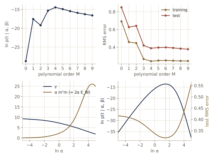
Now let the iteration find both hyperparameters from a poor starting point.
def evidence_maximization(Phi, t, alpha=1.0, beta=1.0, max_iter=200, tol=1e-8, report=()):
    """Fixed-point re-estimation of alpha and beta (Bishop eqs. 3.92 and 3.95)."""
    N = len(t)
    eig = np.linalg.eigvalsh(Phi.T @ Phi)
    history = []
    for it in range(max_iter):
        le, m = log_evidence(Phi, t, alpha, beta)
        lam = beta * eig
        gamma = np.sum(lam / (alpha + lam))
        history.append(le)
        if it in report:
            print(f"  iter {it:2d}: alpha = {alpha:8.4f}  beta = {beta:8.4f}  gamma = {gamma:.4f}  ln evidence = {le:.4f}")
        alpha_new = gamma / (m @ m)
        beta_new = (N - gamma) / np.sum((t - Phi @ m) ** 2)
        converged = abs(alpha_new - alpha) < tol * alpha and abs(beta_new - beta) < tol * beta
        alpha, beta = alpha_new, beta_new
        if converged:
            break
    return alpha, beta, gamma, m, np.array(history)

alpha_hat, beta_hat, gamma_hat, m_hat, hist = evidence_maximization(Phi, t, report=(0, 1, 2, 3, 5))
print(f"converged after {len(hist)} iterations: alpha = {alpha_hat:.4f}, beta = {beta_hat:.4f}, gamma = {gamma_hat:.4f}")
print(f"ln evidence never decreased: {np.all(np.diff(hist) >= -1e-10)}")

grid_a, grid_b = np.linspace(-4, 6, 101), np.linspace(0, 5, 101)
G = np.array([[log_evidence(Phi, t, np.exp(p), np.exp(q))[0] for q in grid_b] for p in grid_a])
i, j = np.unravel_index(np.argmax(G), G.shape)
print(f"grid search: ln alpha = {grid_a[i]:.2f}, ln beta = {grid_b[j]:.2f};  "
      f"iteration: ln alpha = {np.log(alpha_hat):.2f}, ln beta = {np.log(beta_hat):.2f}")
  iter  0: alpha =   1.0000  beta =   1.0000  gamma = 4.9272  ln evidence = -30.2091
  iter  1: alpha =   4.8247  beta =  10.4746  gamma = 5.7495  ln evidence = -13.6318
  iter  2: alpha =   4.4758  beta =  11.1001  gamma = 5.8829  ln evidence = -13.6043
  iter  3: alpha =   4.4061  beta =  11.1635  gamma = 5.9042  ln evidence = -13.6037
  iter  5: alpha =   4.3924  beta =  11.1745  gamma = 5.9083  ln evidence = -13.6037
converged after 11 iterations: alpha = 4.3920, beta = 11.1748, gamma = 5.9084
ln evidence never decreased: True
grid search: ln alpha = 1.50, ln beta = 2.40;  iteration: ln alpha = 1.48, ln beta = 2.41
From \(\alpha = \beta = 1\), a few iterations bring the log evidence from about \(-30\) to its maximum, and the evidence increased at every step. The estimated noise precision, about 11.2, is very close to the true value 11.1 (compare \(\beta_{\mathrm{ML}} \approx 17\) from the maximum likelihood fit), and a brute-force grid search over both hyperparameters lands at the same place. The fixed-point iteration is not guaranteed to increase the evidence at every step in general, but it usually does in practice. The same maximum can also be reached by the EM algorithm, which treats \(\mathbf{w}\) as a latent variable (module 09, Bishop §9.3.4).
The effective number of parameters
What does \(\gamma\) mean? Work in the coordinates of the eigenvectors \(\mathbf{u}_i\). In each such direction, the likelihood curvature is \(\lambda_i\) and the prior curvature is \(\alpha\). The factor \(\lambda_i / (\lambda_i + \alpha)\) lies between 0 and 1:
- If \(\lambda_i \gg \alpha\), the data dominate; the posterior mean in that direction nearly matches the maximum likelihood value, and the factor is near 1. Such a direction is well determined by the data.
- If \(\lambda_i \ll \alpha\), the likelihood is nearly flat in that direction, the prior wins and pulls the weight toward zero, and the factor is near 0.
So \(\gamma = \sum_i \lambda_i / (\lambda_i + \alpha)\), between 0 and \(M\), counts the effective number of parameters: the number of directions in weight space that the data actually determine. The \(\alpha\) equation then reads \(\alpha = \gamma / \mathbf{m}_N^{\mathrm{T}} \mathbf{m}_N\): the prior precision is set so that the well-determined parameters, on average, have the size the prior expects.
The \(\beta\) equation has a similarly clean meaning. Maximum likelihood divides the sum of squared residuals by \(N\); the evidence divides by \(N - \gamma\). This is the regression version of dividing a sample variance by \(N - 1\) instead of \(N\): fitting the mean uses up one degree of freedom, and here fitting the function uses up \(\gamma\) of them. Only the \(\gamma\) well-determined parameters were tuned to the data (and so to its noise); the others were held near zero by the prior.
lam = beta_hat * eig0
ratios = np.sort(lam / (lam + alpha_hat))[::-1]
print("lambda_i / (lambda_i + alpha):", ratios)
print(f"gamma = {ratios.sum():.4f} of M = {len(ratios)}")
rss = np.sum((t - Phi @ m_hat) ** 2)
print(f"noise sd: divide by N -> {np.sqrt(rss / len(t)):.4f};  divide by N - gamma -> {np.sqrt(rss / (len(t) - gamma_hat)):.4f};  true {NOISE_SD}")

xb, tb = sin_data(2000, seed=5)                    # many more data points than parameters
Phib = design_matrix(xb, gauss_basis, MU9, S9)
a_b, b_b, g_b, _, _ = evidence_maximization(Phib, tb)
print(f"N = 2000: gamma = {g_b:.3f} of M = {Phib.shape[1]}, beta = {b_b:.3f}")
lambda_i / (lambda_i + alpha): [0.9896 0.9599 0.9435 0.8898 0.8602 0.6447 0.3697 0.197  0.053  0.0008]
gamma = 5.9084 of M = 10
noise sd: divide by N -> 0.2614;  divide by N - gamma -> 0.2991;  true 0.3
N = 2000: gamma = 8.988 of M = 10, beta = 10.678
With 25 points, about six of the ten directions are well determined and the rest are mostly controlled by the prior. Dividing by \(N - \gamma\) rather than \(N\) moves the noise estimate much closer to the true 0.3. With 2000 points, \(\mathbf{\Phi}^{\mathrm{T}} \mathbf{\Phi}\) is a sum over many more data points, all its eigenvalues grow, and \(\gamma\) rises to about 9 of 10. The one direction still left mostly to the prior is the near-collinear one we met at the start, the bias against the sum of the bumps. As \(N\) keeps growing, \(\gamma\) approaches \(M\), and in that regime (\(N \gg M\)) the re-estimation equations simplify to \(\alpha = M / (2 E_W(\mathbf{m}_N))\) and \(\beta = N / (2 E_D(\mathbf{m}_N))\), which need no eigenvalues at all.
The evidence framework chose \(\alpha\) and \(\beta\) using only the training data: no validation set and no repeated fitting as in cross-validation. The same idea, with a separate \(\alpha_i\) for each weight, drives the relevance vector machine in module 07, where maximizing the evidence switches most basis functions off.
Limitations of fixed basis functions
Linear basis function models have a lot going for them: closed-form least squares, an exact Bayesian treatment, and, with enough basis functions, the ability to represent any reasonable nonlinear function of the input. Module 04 builds the analogous models for classification. Why, then, do later modules move on to neural networks, support vector machines, and relevance vector machines?
The problem is that the basis functions are fixed before we see the data. To cover the input space with, say, \(k\) Gaussian bumps along each axis, we need \(k^D\) of them in \(D\) dimensions: the curse of dimensionality from module 01 again. Worse, most of them would sit where there is no data.
k, N_pts = 5, 1000
g = np.random.default_rng(4)
print("  D    cells (k^D)   cells containing at least one of 1000 points")
for D in [1, 2, 3, 4, 6, 8]:
    X = g.uniform(0, 1, (N_pts, D))
    cells = np.floor(X * k).astype(int) @ (k ** np.arange(D))     # grid cell index of each point
    occupied = len(np.unique(cells))
    print(f"{D:3d}   {k**D:11,d}   {occupied:6d}  ({100 * occupied / k**D:.2f}%)")
  D    cells (k^D)   cells containing at least one of 1000 points
  1             5        5  (100.00%)
  2            25       25  (100.00%)
  3           125      125  (100.00%)
  4           625      493  (78.88%)
  6        15,625      951  (6.09%)
  8       390,625     1000  (0.26%)
With five bumps per axis, eight inputs already require about 390,000 basis functions, and a thousand data points touch well under one percent of the cells. A model with one weight per cell would be hopelessly underdetermined.
Two properties of real data rescue us. First, real inputs rarely fill the input space: strong correlations between the input variables mean the data lie near a lower-dimensional (possibly curved) manifold, as we will see for images of handwritten digits in module 12. Localized basis functions placed only where the data are (radial basis function networks, support vector and relevance vector machines, modules 06–07) exploit this. Second, the target often depends on only a few directions within that manifold. Neural networks (module 05) exploit both properties by learning their basis functions, adapting where they respond and which input directions they respond to.
Everything in this module carries over to those models in some form. Neural networks are trained by gradient methods like LMS and regularized by weight decay; Gaussian processes are the equivalent-kernel view taken seriously; the relevance vector machine is evidence maximization with many hyperparameters. The linear model is the case where we can do everything exactly and see what is going on.
Summary
| Method | What it assumes | How it is fit | What it gives |
|---|---|---|---|
| Least squares / maximum likelihood | \(t = \mathbf{w}^{\mathrm{T}} \boldsymbol{\phi}(\mathbf{x}) +\) Gaussian noise | normal equations, solved with lstsq or QR; LMS sequentially |
\(\mathbf{w}_{\mathrm{ML}} = \mathbf{\Phi}^{\dagger} \mathbf{t}\), \(1/\beta_{\mathrm{ML}}\) = mean squared residual |
| Ridge regression | plus a quadratic penalty \(\frac{\lambda}{2} \mathbf{w}^{\mathrm{T}} \mathbf{w}\) | one linear solve | \((\lambda \mathbf{I} + \mathbf{\Phi}^{\mathrm{T}} \mathbf{\Phi})^{-1} \mathbf{\Phi}^{\mathrm{T}} \mathbf{t}\); shrunken weights |
| Lasso | plus \(\frac{\lambda}{2} \sum_j \lvert w_j \rvert\) | coordinate descent with soft thresholding | sparse weights |
| Bayesian linear regression | Gaussian prior \(\mathcal{N}(\mathbf{0}, \alpha^{-1} \mathbf{I})\), known \(\alpha, \beta\) | closed form, batch or sequential | posterior \(\mathcal{N}(\mathbf{m}_N, \mathbf{S}_N)\); predictive variance \(1/\beta + \boldsymbol{\phi}^{\mathrm{T}} \mathbf{S}_N \boldsymbol{\phi}\) |
| Evidence approximation | flat hyperprior, peaked \(p(\alpha, \beta \mid \mathbf{t})\) | fixed-point iteration on \(\alpha = \gamma / \mathbf{m}_N^{\mathrm{T}} \mathbf{m}_N\), \(1/\beta = \text{RSS}/(N - \gamma)\) | \(\hat{\alpha}, \hat{\beta}\) and the effective number of parameters \(\gamma\) |
Ideas to carry forward:
- Linearity in the parameters is what makes these models tractable: the likelihood is quadratic in \(\mathbf{w}\), so least squares is a linear solve and a Gaussian prior gives an exact Gaussian posterior. Good numerics (avoid forming inverses, watch the condition number) matter as much as the formulas.
- Overfitting is a variance problem. Regularization trades variance for bias; the Bayesian view reads the regularizer as a prior, with \(\lambda = \alpha / \beta\), and replaces a single weight vector with an average over the posterior.
- The predictive distribution separates irreducible noise (\(1/\beta\)) from uncertainty about the weights, which shrinks with data. The equivalent kernel shows the prediction as a weighted sum of training targets, pointing ahead to kernel methods and Gaussian processes.
- The model evidence rewards fit and penalizes needless flexibility automatically. Maximizing it over the hyperparameters chooses the complexity from the training data alone, and \(\gamma\) counts how many parameters the data really determine.
Exercises
- Weighted least squares. Suppose each target has its own known noise precision, \(t_n \sim \mathcal{N}(\mathbf{w}^{\mathrm{T}} \boldsymbol{\phi}(\mathbf{x}_n), (\beta r_n)^{-1})\) with weights \(r_n > 0\). Write down the log likelihood, derive the maximum likelihood weights in terms of \(\mathbf{\Phi}\), \(\mathbf{t}\), and \(\mathbf{R} = \operatorname{diag}(r_1, \dots, r_N)\), and show how to compute them with
fit_mlby rescaling the rows of \(\mathbf{\Phi}\) and \(\mathbf{t}\). Check your formula numerically. - Show that the hat matrix \(\mathbf{H} = \mathbf{\Phi} (\mathbf{\Phi}^{\mathrm{T}} \mathbf{\Phi})^{-1} \mathbf{\Phi}^{\mathrm{T}}\) satisfies \(\mathbf{H}^2 = \mathbf{H}\), \(\mathbf{H}^{\mathrm{T}} = \mathbf{H}\), and \(\operatorname{tr} \mathbf{H} = M\). Then show that for ridge regression the analogous matrix \(\mathbf{H}_\lambda = \mathbf{\Phi} (\lambda \mathbf{I} + \mathbf{\Phi}^{\mathrm{T}} \mathbf{\Phi})^{-1} \mathbf{\Phi}^{\mathrm{T}}\) is not a projection, and that its trace equals \(\gamma\) from the evidence section when \(\lambda = \alpha / \beta\). Verify with the running data.
- For LMS on a fixed data set, show that if the learning rate is constant and the data can be fit exactly (\(\mathbf{t} = \mathbf{\Phi} \mathbf{w}^\star\) for some \(\mathbf{w}^\star\)), the iteration can converge to \(\mathbf{w}^\star\) without any decay. Test it: generate exact targets from the three-parameter model and run
lmswith \(\eta = 0.5\). Why does noise in the targets change the picture? - Compute the whole lasso path for the running data: the weights of
fit_lassofor 60 values of \(\ln \lambda\) between \(-6\) and \(3\), starting each fit from the previous solution (a “warm start”; add an initial-weights argument). Plot each weight against \(\ln \lambda\) and report the order in which the basis functions leave the model. How much does the warm start reduce the total number of sweeps? - Show that for an orthonormal design (\(\mathbf{\Phi}^{\mathrm{T}} \mathbf{\Phi} = \mathbf{I}\)) the ridge solution is \(\mathbf{w}_{\mathrm{ML}} / (1 + \lambda)\) and the lasso solution is the soft threshold of \(\mathbf{w}_{\mathrm{ML}}\) at \(\lambda / 2\), component by component. Sketch both as functions of one component of \(\mathbf{w}_{\mathrm{ML}}\) and explain the difference between shrinking and selecting.
- Repeat the bias–variance experiment with the number of Gaussian bumps as the complexity knob instead of \(\lambda\): use \(k = 1, 2, \dots, 20\) evenly spaced bumps with width equal to their spacing, a tiny fixed \(\lambda = 10^{-6}\), and the same 100 data sets. Plot bias², variance, and test error against \(k\). Is the picture the same as for \(\lambda\)?
- Derive the posterior of Bayesian linear regression a second way, from the linear-Gaussian formulas of module 02: treat \(\mathbf{w}\) as the “hidden” Gaussian variable and \(\mathbf{t} = \mathbf{\Phi} \mathbf{w} + \boldsymbol{\epsilon}\) as the observation. Check that you recover \(\mathbf{m}_N\) and \(\mathbf{S}_N\) for a general prior mean \(\mathbf{m}_0\) and covariance \(\mathbf{S}_0\).
- Prove that \(\sigma_{N+1}^2(\mathbf{x}) \le \sigma_N^2(\mathbf{x})\). (Hint: write \(\mathbf{S}_{N+1}^{-1} = \mathbf{S}_N^{-1} + \beta \boldsymbol{\phi}_{N+1} \boldsymbol{\phi}_{N+1}^{\mathrm{T}}\) and the Woodbury identity from Bishop’s Appendix C, in its rank-one form.) By how much does the variance drop at the new input \(\mathbf{x}_{N+1}\) itself?
- Using the equivalent kernel, show that the vector of fitted values on the training inputs is \(\mathbf{K} \mathbf{t}\) with \(\mathbf{K} = \beta \mathbf{\Phi} \mathbf{S}_N \mathbf{\Phi}^{\mathrm{T}}\), and prove that \(\operatorname{tr} \mathbf{K} = \gamma\). Compute both sides for the running data at the evidence optimum.
- Show that at the evidence optimum \(2 E(\mathbf{m}_N) = N\), where \(E(\mathbf{w}) = \beta E_D(\mathbf{w}) + \alpha E_W(\mathbf{w})\). (Add the two re-estimation equations.) Check it numerically with
alpha_hat,beta_hat, andm_hat. - Use the evidence to choose the width \(s\) of the 9 Gaussian bumps: for each \(s\) in a grid from 0.02 to 0.5, run
evidence_maximizationand record the maximized log evidence. Which width does the evidence prefer, and how does the test RMS behave across the same grid? - In your own words: explain to a classmate why maximizing the likelihood over \(\mathbf{w}\) overfits, but maximizing the evidence over \(\alpha\) and \(\beta\) does not. Where in the log-evidence formula does the protection against overfitting come from?
Going further
- C. M. Bishop, Pattern Recognition and Machine Learning, chapter 3 — the source for this module. Exercises 3.2 (projection), 3.5 (the lasso as a constrained problem), 3.7–3.10 (posterior and predictive distribution), 3.11 (shrinking predictive variance), 3.14 (the equivalent kernel with an orthonormal basis), 3.16–3.22 (deriving and maximizing the evidence) are good companions to the notes.
- David J. C. MacKay, “Bayesian interpolation”, Neural Computation, 1992 — the paper that brought the evidence framework, and the effective number of parameters, to machine learning.
- Robert Tibshirani, “Regression shrinkage and selection via the lasso”, Journal of the Royal Statistical Society, Series B, 1996 — the original lasso paper.
- Jerome Friedman, Trevor Hastie, and Robert Tibshirani, “Regularization paths for generalized linear models via coordinate descent”, Journal of Statistical Software, 2010 — coordinate descent for the lasso and its relatives, at scale.
- Trevor Hastie, Robert Tibshirani, and Jerome Friedman, The Elements of Statistical Learning, 2nd ed., Springer, 2009 (free PDF) — chapter 3 covers least squares, ridge, the lasso, and their geometry from the statistician’s side.
These notes follow the chapters of C. M. Bishop, Pattern Recognition and Machine Learning (Springer, 2006), the course text, which Microsoft Research makes freely available as a PDF. The explanations, code, figures, and exercises here are written for this course; the book remains the reference, with the full derivations and many more exercises.