CSE 474/574 · Module 07 · Week 7
Sparse Kernel Machines: SVMs and RVMs
Maximum-margin classifiers, soft margins and the hinge loss, support vector regression, and the relevance vector machine.
Companion reading: Bishop, Pattern Recognition and Machine Learning, chapter 7, “Sparse Kernel Machines”
By the end of this module you can
- Derive the maximum-margin problem for a linear classifier in feature space, form its Lagrangian, and obtain the dual problem in terms of a kernel.
- Use the Karush–Kuhn–Tucker conditions to explain why an SVM’s predictions depend only on its support vectors, and how to recover the bias \(b\).
- Implement a sequential minimal optimization (SMO) solver for the SVM dual in NumPy and check it against a generic optimizer.
- Explain slack variables, the box constraint \(0 \le a_n \le C\), and how \(C\) trades training error against margin, and read off the three kinds of training point from a solution.
- Compare the hinge, logistic, squared, and misclassification losses, and say why the hinge loss produces sparse solutions.
- Set up support vector regression with the \(\epsilon\)-insensitive loss, solve its dual with the same SMO code, and describe the multiclass options and their problems.
- State what PAC learning and the VC dimension measure, and why the resulting bounds are loose in practice.
- Fit a relevance vector machine by evidence maximization, explain its sparsity through the sparsity and quality factors \(s_i\) and \(q_i\), and compare it with the SVM for regression and classification.
Contents
- Constrained optimization in one page
- Maximum margin classifiers
- Overlapping classes: the soft margin
- Relation to logistic regression
- Multiclass SVMs
- SVMs for regression
- Computational learning theory
- Relevance vector machines
- Summary
- Exercises
- Going further
In module 06 we rewrote linear models in terms of a kernel \(k(\mathbf{x}, \mathbf{x}')\) and met Gaussian processes. Those methods are powerful, but they have a cost that grows with the data: a Gaussian process prediction at a new input needs the kernel between that input and every training point, and training needs an \(N \times N\) matrix. With a hundred thousand training points, that is a problem at prediction time as well as at training time.
This module is about kernel machines whose solutions are sparse: once trained, a prediction uses the kernel at only a subset of the training points, and the rest of the training set can be thrown away. We look at two such machines. The support vector machine (SVM) gets its sparsity from geometry and convex optimization: it places the decision boundary as far as possible from the data, and only the points closest to the boundary end up mattering. The relevance vector machine (RVM) gets its sparsity from Bayesian model selection: it gives every weight its own prior precision and lets the evidence switch most of the weights off.
Both build on earlier modules. The SVM is a linear classifier in feature space, like the models of module 04, and its loss function turns out to be a close cousin of the logistic regression loss. The RVM is Bayesian linear regression from module 03, with the evidence approximation doing the work, plus the Laplace approximation of module 04 for classification. Everything is implemented in NumPy: we write our own solver for the SVM’s quadratic program, and our own evidence maximization for the RVM.
Constrained optimization in one page
The SVM is defined as the solution of an optimization problem with inequality constraints, so we first collect the tools we need. Bishop’s Appendix E has a longer, geometric treatment.
Equality constraints. To minimize \(f(\mathbf{x})\) subject to \(g(\mathbf{x}) = 0\), form the Lagrangian \(L(\mathbf{x}, \lambda) = f(\mathbf{x}) - \lambda g(\mathbf{x})\) and look for points where \(\nabla_{\mathbf{x}} L = 0\) and \(g(\mathbf{x}) = 0\). The first condition says \(\nabla f = \lambda \nabla g\): at a constrained optimum the gradient of \(f\) is perpendicular to the constraint surface, since otherwise we could slide along the surface and decrease \(f\). The number \(\lambda\) is a Lagrange multiplier; for an equality constraint it can have either sign.
Inequality constraints. Now minimize \(f(\mathbf{x})\) subject to \(g(\mathbf{x}) \ge 0\). Either the minimum lies strictly inside the feasible region, where the constraint is inactive and plays no role (\(\nabla f = 0\)), or it lies on the boundary \(g(\mathbf{x}) = 0\), where the constraint is active. In the active case, \(f\) must increase as we move into the feasible region, so \(\nabla f\) points the same way as \(\nabla g\): \(\nabla f = \lambda \nabla g\) with \(\lambda \ge 0\). Both cases are captured by one set of conditions.
Definition. For the problem “minimize \(f(\mathbf{x})\) subject to \(g_k(\mathbf{x}) \ge 0\), \(k = 1, \dots, K\)”, form \(L(\mathbf{x}, \boldsymbol{\lambda}) = f(\mathbf{x}) - \sum_k \lambda_k g_k(\mathbf{x})\). The Karush–Kuhn–Tucker (KKT) conditions are: stationarity \(\nabla_{\mathbf{x}} L = 0\); feasibility \(g_k(\mathbf{x}) \ge 0\); nonnegative multipliers \(\lambda_k \ge 0\); and complementary slackness \(\lambda_k g_k(\mathbf{x}) = 0\) for every \(k\).
Complementary slackness is the condition to remember: for each constraint, either the constraint is active or its multiplier is zero. An inactive constraint has no say in the solution.
Duality. For a fixed \(\boldsymbol{\lambda} \ge 0\), minimize the Lagrangian over \(\mathbf{x}\) without any constraints. The result, \(\widetilde{L}(\boldsymbol{\lambda}) = \min_{\mathbf{x}} L(\mathbf{x}, \boldsymbol{\lambda})\), is the dual function. For any feasible \(\mathbf{x}\) we have \(L(\mathbf{x}, \boldsymbol{\lambda}) \le f(\mathbf{x})\), because we subtract nonnegative terms, so \(\widetilde{L}(\boldsymbol{\lambda})\) is a lower bound on the constrained minimum. The dual problem maximizes this bound over \(\boldsymbol{\lambda} \ge 0\). When \(f\) is convex and the constraints are linear, as they will be for the SVM, the best bound is tight: the maximum of the dual equals the minimum of the original, primal, problem, and the two solutions together satisfy the KKT conditions.
A one-line example that already has the shape of an SVM: minimize \(\tfrac12 (x_1^2 + x_2^2)\) subject to \(x_1 + x_2 - 1 \ge 0\). The Lagrangian is \(\tfrac12 \lVert \mathbf{x} \rVert^2 - \lambda (x_1 + x_2 - 1)\). Setting its gradient to zero gives \(\mathbf{x} = \lambda (1, 1)^{\mathrm{T}}\), and substituting back gives the dual function \(\widetilde{L}(\lambda) = \lambda - \lambda^2\). It is maximized at \(\lambda = \tfrac12\), so \(\mathbf{x} = (\tfrac12, \tfrac12)\) and both problems have the value \(\tfrac14\). The constraint is active and its multiplier is positive. If the constraint were \(x_1 + x_2 + 1 \ge 0\) instead, the unconstrained minimum \(\mathbf{x} = \mathbf{0}\) would already be feasible, the constraint would be inactive, and its multiplier would be zero.
Maximum margin classifiers
The margin of a linear classifier
We return to two-class classification with a linear model in a fixed feature space,
\[y(\mathbf{x}) = \mathbf{w}^{\mathrm{T}} \boldsymbol{\phi}(\mathbf{x}) + b,\]with the bias \(b\) written separately from \(\mathbf{w}\). The targets are coded as \(t_n \in \{-1, +1\}\) (not \(\{0, 1\}\) as in logistic regression), and a new input is assigned to the class given by the sign of \(y(\mathbf{x})\). With this coding, a training point is classified correctly exactly when \(t_n y(\mathbf{x}_n) > 0\).
Suppose for now that the training set is linearly separable in feature space: some choice of \(\mathbf{w}\) and \(b\) gives \(t_n y(\mathbf{x}_n) > 0\) for every \(n\). Then there are usually infinitely many separating hyperplanes. The perceptron of module 04 finds one of them, but which one depends on the starting point and the order in which it visits the data. We would like a principled choice, one that we expect to classify new points well.
The SVM’s choice is the hyperplane with the largest margin, the distance from the decision boundary to the closest training point. The intuition is robustness: a boundary that passes close to some training point would misclassify a test point that differs from it only slightly, while a boundary with a wide empty corridor on both sides leaves room for such variation. The section on learning theory below gives a more formal motivation.
Recall from module 04 that the perpendicular distance from a point \(\mathbf{x}\) to the hyperplane \(y(\mathbf{x}) = 0\) is \(\lvert y(\mathbf{x}) \rvert / \lVert \mathbf{w} \rVert\), measured in feature space. For a correctly classified point, \(\lvert y(\mathbf{x}_n) \rvert = t_n y(\mathbf{x}_n)\), so its distance to the boundary is
\[\frac{t_n y(\mathbf{x}_n)}{\lVert \mathbf{w} \rVert} = \frac{t_n \left( \mathbf{w}^{\mathrm{T}} \boldsymbol{\phi}(\mathbf{x}_n) + b \right)}{\lVert \mathbf{w} \rVert}.\]The margin is the smallest of these distances, and the maximum margin classifier solves
\[\max_{\mathbf{w}, b} \left\{ \frac{1}{\lVert \mathbf{w} \rVert} \min_{n} \, t_n \left( \mathbf{w}^{\mathrm{T}} \boldsymbol{\phi}(\mathbf{x}_n) + b \right) \right\}.\]The primal problem
That max–min problem is awkward to optimize directly. The trick is to notice that \(\mathbf{w}\) and \(b\) have a redundant scale: replacing them by \(\kappa \mathbf{w}\) and \(\kappa b\) for any \(\kappa > 0\) gives the same hyperplane and the same distances. We can therefore fix the scale by requiring that the closest point has \(t_n y(\mathbf{x}_n) = 1\). Every point then satisfies
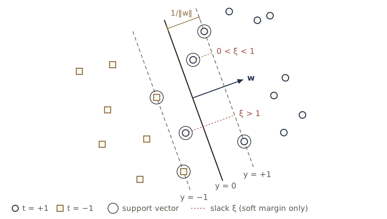
\[t_n \left( \mathbf{w}^{\mathrm{T}} \boldsymbol{\phi}(\mathbf{x}_n) + b \right) \ge 1, \qquad n = 1, \dots, N,\]and the margin is simply \(1 / \lVert \mathbf{w} \rVert\). This is called the canonical representation of the hyperplane. The two hyperplanes \(y(\mathbf{x}) = +1\) and \(y(\mathbf{x}) = -1\) are the margin boundaries; no training point lies strictly between them. Maximizing \(1 / \lVert \mathbf{w} \rVert\) is the same as minimizing \(\lVert \mathbf{w} \rVert^2\), so we arrive at the primal problem.
The hard-margin SVM therefore solves: minimize \(\tfrac12 \lVert \mathbf{w} \rVert^2\) over \(\mathbf{w}\) and \(b\), subject to \(t_n \left( \mathbf{w}^{\mathrm{T}} \boldsymbol{\phi}(\mathbf{x}_n) + b \right) \ge 1\) for \(n = 1, \dots, N\).
This is a quadratic program: a convex quadratic objective with linear inequality constraints. It has a unique minimizer \(\mathbf{w}\), and no local minima to get stuck in. The bias \(b\) does not appear in the objective, but it is pinned down by the constraints, since changing \(b\) shifts the hyperplane toward one class or the other. A constraint that holds with equality is active; the corresponding points sit exactly on a margin boundary.
The Lagrangian and the dual
Following the recipe of the previous section, we introduce one multiplier \(a_n \ge 0\) for each constraint and form
\[L(\mathbf{w}, b, \mathbf{a}) = \frac12 \lVert \mathbf{w} \rVert^2 - \sum_{n=1}^{N} a_n \left\{ t_n \left( \mathbf{w}^{\mathrm{T}} \boldsymbol{\phi}(\mathbf{x}_n) + b \right) - 1 \right\}.\]We minimize over \(\mathbf{w}\) and \(b\). Setting the derivatives to zero gives two conditions:
\[\frac{\partial L}{\partial \mathbf{w}} = 0 \;\Rightarrow\; \mathbf{w} = \sum_{n=1}^{N} a_n t_n \boldsymbol{\phi}(\mathbf{x}_n), \qquad \frac{\partial L}{\partial b} = 0 \;\Rightarrow\; \sum_{n=1}^{N} a_n t_n = 0.\]The first says that the optimal weight vector is a combination of the training feature vectors, the same dual representation we met in module 06. To eliminate \(\mathbf{w}\) and \(b\), expand the Lagrangian. The term in \(b\) is \(-b \sum_n a_n t_n = 0\), and \(\sum_n a_n t_n \mathbf{w}^{\mathrm{T}} \boldsymbol{\phi}(\mathbf{x}_n) = \mathbf{w}^{\mathrm{T}} \mathbf{w}\) by the first condition, so
\[L = \frac12 \lVert \mathbf{w} \rVert^2 - \lVert \mathbf{w} \rVert^2 + \sum_n a_n = \sum_{n=1}^{N} a_n - \frac12 \sum_{n=1}^{N} \sum_{m=1}^{N} a_n a_m t_n t_m k(\mathbf{x}_n, \mathbf{x}_m),\]where \(k(\mathbf{x}, \mathbf{x}') = \boldsymbol{\phi}(\mathbf{x})^{\mathrm{T}} \boldsymbol{\phi}(\mathbf{x}')\) and we used \(\lVert \mathbf{w} \rVert^2 = \sum_n \sum_m a_n a_m t_n t_m k(\mathbf{x}_n, \mathbf{x}_m)\).
Result. The dual of the hard-margin SVM: maximize \(\widetilde{L}(\mathbf{a}) = \sum_n a_n - \tfrac12 \sum_n \sum_m a_n a_m t_n t_m k(\mathbf{x}_n, \mathbf{x}_m)\) subject to \(a_n \ge 0\) and \(\sum_n a_n t_n = 0\). Predictions use \(y(\mathbf{x}) = \sum_n a_n t_n k(\mathbf{x}, \mathbf{x}_n) + b\).
The feature vectors have disappeared: only kernel values remain. That is the point of the dual. The primal problem has one variable per feature (plus \(b\)), the dual one variable per data point. If the feature space has fewer dimensions than there are data points, the dual looks like a bad trade, since a general quadratic program costs roughly the cube of its number of variables. But the dual lets us use any valid kernel, including the Gaussian kernel, whose feature space is infinite-dimensional, where the primal cannot even be written down. The requirement from module 06 that the kernel be positive semidefinite is what makes the dual objective concave, so that it has a well-defined maximum.
In matrix form, with \(\mathbf{Q}\) the \(N \times N\) matrix with entries \(Q_{nm} = t_n t_m k(\mathbf{x}_n, \mathbf{x}_m)\), the dual objective is \(\mathbf{1}^{\mathrm{T}} \mathbf{a} - \tfrac12 \mathbf{a}^{\mathrm{T}} \mathbf{Q} \mathbf{a}\).
KKT conditions: why only the support vectors matter
The primal problem is convex with linear constraints, so its solution satisfies the KKT conditions. Here they read
\[a_n \ge 0, \qquad t_n y(\mathbf{x}_n) - 1 \ge 0, \qquad a_n \left\{ t_n y(\mathbf{x}_n) - 1 \right\} = 0.\]By complementary slackness, every training point has either \(a_n = 0\) or \(t_n y(\mathbf{x}_n) = 1\). A point with \(a_n = 0\) drops out of the sum in \(y(\mathbf{x})\) and has no influence on any prediction. The points with \(a_n > 0\) are the support vectors, and they all lie exactly on a margin boundary. This is where the sparsity of the SVM comes from: typically most points sit comfortably away from the boundary, their constraints are inactive, and their multipliers are zero.
To find \(b\), use any support vector: \(t_n y(\mathbf{x}_n) = 1\) and \(t_n^2 = 1\) give \(b = t_n - \sum_m a_m t_m k(\mathbf{x}_n, \mathbf{x}_m)\). Each support vector gives the same value in exact arithmetic; numerically it is better to average over all of them,
\[b = \frac{1}{N_{\mathcal{S}}} \sum_{n \in \mathcal{S}} \left( t_n - \sum_{m \in \mathcal{S}} a_m t_m k(\mathbf{x}_n, \mathbf{x}_m) \right),\]where \(\mathcal{S}\) is the set of support vectors and \(N_{\mathcal{S}}\) its size.
The same conditions give a neat formula for the margin. Multiply each complementary slackness condition out and add them up: \(\sum_n a_n t_n (\mathbf{w}^{\mathrm{T}} \boldsymbol{\phi}(\mathbf{x}_n) + b) = \sum_n a_n\). The left side is \(\mathbf{w}^{\mathrm{T}} \mathbf{w} + b \sum_n a_n t_n = \lVert \mathbf{w} \rVert^2\). So at the solution \(\lVert \mathbf{w} \rVert^2 = \sum_n a_n\), and the margin is \(\rho = 1 / \sqrt{\sum_n a_n}\). We will check this in code.
Written as the minimization of an error function, the hard-margin SVM minimizes \(\sum_n E_\infty(t_n y(\mathbf{x}_n) - 1) + \lambda \lVert \mathbf{w} \rVert^2\), where \(E_\infty(z)\) is zero for \(z \ge 0\) and infinite otherwise. The infinite penalty enforces the constraints, and any \(\lambda > 0\) gives the same answer. We come back to this form when we compare the SVM with logistic regression.
Solving the dual: sequential minimal optimization
The dual is a quadratic program in \(N\) variables. A general-purpose QP solver works for small \(N\) but needs the whole \(N \times N\) matrix \(\mathbf{Q}\) in memory and time roughly cubic in \(N\). The most widely used SVM training method, sequential minimal optimization (SMO), due to Platt, goes to the other extreme: it changes only two multipliers at a time. Two is the smallest number that works, because the equality constraint \(\sum_n a_n t_n = 0\) would undo any change to a single multiplier. With two variables, the subproblem can be solved in closed form.
We write the solver once for a slightly more general problem, because support vector regression later in the module has the same shape:
\[\min_{\boldsymbol{\beta}} \; \frac12 \boldsymbol{\beta}^{\mathrm{T}} \mathbf{Q} \boldsymbol{\beta} + \mathbf{p}^{\mathrm{T}} \boldsymbol{\beta} \quad \text{subject to} \quad \sum_n z_n \beta_n = 0, \quad 0 \le \beta_n \le C,\]with \(Q_{nm} = z_n z_m \widetilde{K}_{nm}\) and every \(z_n \in \{-1, +1\}\). The hard-margin dual is the case \(\boldsymbol{\beta} = \mathbf{a}\), \(\mathbf{z} = \mathbf{t}\), \(\widetilde{\mathbf{K}} = \mathbf{K}\), \(\mathbf{p} = -\mathbf{1}\), and \(C = \infty\) (we minimize the negative of \(\widetilde{L}\)). The finite \(C\) will appear in the next section.
One step. Let \(\mathbf{G} = \mathbf{Q} \boldsymbol{\beta} + \mathbf{p}\) be the gradient of the objective, and define \(v_n = -z_n G_n\). Pick two indices \(i \neq j\) and move along the direction that keeps \(\sum_n z_n \beta_n\) fixed: \(\beta_i \leftarrow \beta_i + z_i \lambda\) and \(\beta_j \leftarrow \beta_j - z_j \lambda\). Along this line the objective changes by
\[\lambda \left( z_i G_i - z_j G_j \right) + \frac{\lambda^2}{2} \eta_{ij} = -\lambda \left( v_i - v_j \right) + \frac{\lambda^2}{2} \eta_{ij}, \qquad \eta_{ij} = \widetilde{K}_{ii} + \widetilde{K}_{jj} - 2 \widetilde{K}_{ij},\]a one-dimensional quadratic. If \(v_i > v_j\), a small step with \(\lambda > 0\) decreases the objective, and the best step is \(\lambda = (v_i - v_j) / \eta_{ij}\), cut back if necessary so that both variables stay inside \([0, C]\). The objective then drops by \((v_i - v_j)^2 / (2 \eta_{ij})\) when the step is not cut back.
Which pair. A step with \(\lambda > 0\) must be allowed to move \(\beta_i\) in the direction \(z_i\) and \(\beta_j\) in the direction \(-z_j\). Call \(I_{\text{up}}\) the indices whose \(\beta_n\) can move in direction \(z_n\) (\(\beta_n < C\) if \(z_n = +1\), \(\beta_n > 0\) if \(z_n = -1\)), and \(I_{\text{low}}\) those that can move in direction \(-z_n\). We take \(i\) to maximize \(v_i\) over \(I_{\text{up}}\), and then \(j \in I_{\text{low}}\) to maximize the guaranteed decrease \((v_i - v_j)^2 / \eta_{ij}\) among those with \(v_j < v_i\). (This second-order choice of \(j\) is the one used in the LIBSVM library; Platt’s original paper uses different heuristics.)
When to stop. Writing out the KKT conditions of this QP, with a multiplier \(b\) for the equality constraint, shows that \(\boldsymbol{\beta}\) is optimal exactly when there is a number \(b\) with \(v_n \le b\) for all \(n \in I_{\text{up}}\) and \(v_n \ge b\) for all \(n \in I_{\text{low}}\), that is, when \(\max_{I_{\text{up}}} v_n \le \min_{I_{\text{low}}} v_n\). So we stop when the largest violation, \(\max_{I_{\text{up}}} v - \min_{I_{\text{low}}} v\), falls below a tolerance. The multiplier \(b\) turns out to be the SVM bias: for the classification dual, \(v_n = t_n - \sum_m a_m t_m k(\mathbf{x}_n, \mathbf{x}_m)\), which is exactly the quantity averaged in the formula for \(b\) above. So at the end we average \(v_n\) over the multipliers strictly inside \((0, C)\).
Keeping it cheap. After a step only two entries of \(\boldsymbol{\beta}\) change, so the gradient is updated with two columns of the kernel matrix: \(\mathbf{G} \leftarrow \mathbf{G} + \lambda\, \mathbf{z} \odot (\widetilde{\mathbf{K}}_{:,i} - \widetilde{\mathbf{K}}_{:,j})\), where \(\odot\) is the elementwise product. Each iteration costs \(O(N)\).
All the code in this module shares one namespace. We import what we need and create a seeded random generator once; every data set below also comes from its own seeded generator, so all outputs are repeatable.
import math
from itertools import product

import numpy as np
from scipy.special import expit                    # the logistic sigmoid
from scipy.linalg import cho_factor, cho_solve

np.set_printoptions(precision=4, suppress=True)
rng = np.random.default_rng(574)
Here is the kernel (vectorized over pairs of rows) and the solver.
def gaussian_kernel(X1, X2, gamma):
    """k(x, x') = exp(-gamma ||x - x'||^2) for every pair of rows of X1 (N1, D) and X2 (N2, D)."""
    sq = (X1 ** 2).sum(1)[:, None] + (X2 ** 2).sum(1)[None, :] - 2 * X1 @ X2.T
    return np.exp(-gamma * np.maximum(sq, 0.0))

def smo(Kt, z, p, C, tol=1e-3, max_iter=200_000):
    """Minimize 0.5 beta^T Q beta + p^T beta,  Q_nm = z_n z_m Kt_nm,
    subject to sum_n z_n beta_n = 0 and 0 <= beta_n <= C, two variables at a time.
    Returns (beta, b, iterations)."""
    n = len(z)
    beta = np.zeros(n)
    G = p.astype(float).copy()                     # gradient Q beta + p, at beta = 0
    for it in range(max_iter):
        v = -z * G
        up = ((z > 0) & (beta < C)) | ((z < 0) & (beta > 0))
        low = ((z < 0) & (beta < C)) | ((z > 0) & (beta > 0))
        iu, il = np.flatnonzero(up), np.flatnonzero(low)
        i = iu[np.argmax(v[iu])]                   # most violating "up" index
        if v[i] - v[il].min() < tol:               # KKT conditions hold to within tol
            break
        gap = v[i] - v[il]                         # candidates j with gap > 0 improve the objective
        eta = np.maximum(Kt[i, i] + Kt[il, il] - 2 * Kt[i, il], 1e-12)
        gain = np.where(gap > 0, gap ** 2 / eta, -np.inf)   # decrease of the objective (times 2)
        k = np.argmax(gain)
        j, eta = il[k], eta[k]
        lam = gap[k] / eta
        lam = min(lam, C - beta[i] if z[i] > 0 else beta[i],
                  beta[j] if z[j] > 0 else C - beta[j])
        beta[i] += z[i] * lam
        beta[j] -= z[j] * lam
        G += lam * z * (Kt[:, i] - Kt[:, j])
    v = -z * G
    free = (beta > 1e-8) & (beta < C - 1e-8)       # 0 < beta_n < C
    if free.any():
        b = v[free].mean()
    else:
        up = ((z > 0) & (beta < C)) | ((z < 0) & (beta > 0))
        low = ((z < 0) & (beta < C)) | ((z > 0) & (beta > 0))
        b = 0.5 * (v[up].max() + v[low].min())
    return beta, b, it
A first test uses a linear kernel, \(k(\mathbf{x}, \mathbf{x}') = \mathbf{x}^{\mathrm{T}} \mathbf{x}'\), so that \(\boldsymbol{\phi}(\mathbf{x}) = \mathbf{x}\) and we can form \(\mathbf{w}\) explicitly. The data are two clouds of 10 points each, far enough apart to be separable.
def make_linear(N, seed):
    """Two Gaussian clouds in 2-D centered at (1, 1) and (-1, -1); labels +1 and -1."""
    g = np.random.default_rng(seed)
    t = np.where(np.arange(N) < N // 2, 1.0, -1.0)
    X = 0.6 * g.standard_normal((N, 2)) + np.outer(t, [1.0, 1.0])
    return X, t

X_lin, t_lin = make_linear(20, seed=1)
K_lin = X_lin @ X_lin.T                         # linear kernel
a, b, iters = smo(K_lin, t_lin, -np.ones(20), C=np.inf, tol=1e-6)
w = (a * t_lin) @ X_lin                         # w = sum_n a_n t_n x_n
sv = np.flatnonzero(a > 1e-8)
print("SMO iterations:", iters)
print("support vectors:", sv, "  a =", a[sv])
print("w =", w, f"  b = {b:.4f}   sum a_n t_n = {a @ t_lin:.1e}")
print("four smallest t_n y(x_n):", np.sort(t_lin * (X_lin @ w + b))[:4])
print(f"||w||^2 = {w @ w:.4f}   sum a_n = {a.sum():.4f}   margin = {1 / np.linalg.norm(w):.4f}")
SMO iterations: 10
support vectors: [ 1  9 11]   a = [0.3252 0.6647 0.99  ]
w = [0.9639 1.0251]   b = -0.3786   sum a_n t_n = 0.0e+00
four smallest t_n y(x_n): [1.     1.     1.     1.0843]
||w||^2 = 1.9800   sum a_n = 1.9799   margin = 0.7107
Everything the theory promised is visible. Only three of the twenty multipliers are nonzero. Exactly three points have \(t_n y(\mathbf{x}_n) = 1\), they are the support vectors, and every other point is strictly outside the margin. The equality constraint holds, and \(\lVert \mathbf{w} \rVert^2 = \sum_n a_n\) as derived above, up to the solver’s tolerance.
A nonlinear boundary with a Gaussian kernel
Now the real use: a Gaussian kernel \(k(\mathbf{x}, \mathbf{x}') = \exp(-\gamma \lVert \mathbf{x} - \mathbf{x}' \rVert^2)\). (Bishop writes it as \(\exp(-\lVert \mathbf{x} - \mathbf{x}' \rVert^2 / 2\sigma^2)\), so \(\gamma = 1/(2\sigma^2)\).) The data set below has two classes separated by a sine-shaped curve, with a thin band around the curve left empty, so that the classes are separable, though not by a straight line.
def make_wave(N, gap, seed):
    """Points in [-2, 2]^2 labeled by their side of the curve x2 = 0.9 sin(1.7 x1).
    Points closer than `gap` (vertically) to the curve are dropped, so the classes are separable."""
    g = np.random.default_rng(seed)
    X = g.uniform(-2, 2, size=(20 * N, 2))
    d = X[:, 1] - 0.9 * np.sin(1.7 * X[:, 0])
    keep = np.abs(d) > gap
    X, d = X[keep][:N], d[keep][:N]
    return X, np.where(d > 0, 1.0, -1.0)

def svm_fit(X, t, C, gamma, tol=1e-3):
    """SVM with a Gaussian kernel (C = np.inf gives the hard margin)."""
    K = gaussian_kernel(X, X, gamma)
    a, b, iters = smo(K, t, -np.ones(len(t)), C, tol)
    sv = a > 1e-8
    return {"X": X[sv], "at": a[sv] * t[sv], "b": b, "gamma": gamma, "C": C,
            "a": a, "iters": iters}

def svm_decision(model, Xnew):
    """y(x) = sum over the support vectors of a_n t_n k(x, x_n) + b."""
    return gaussian_kernel(Xnew, model["X"], model["gamma"]) @ model["at"] + model["b"]

X_wave, t_wave = make_wave(80, gap=0.3, seed=3)
hard = svm_fit(X_wave, t_wave, C=np.inf, gamma=1.0, tol=1e-6)
ty = t_wave * svm_decision(hard, X_wave)
on_margin = hard["a"] > 1e-8
print("points per class:", int((t_wave > 0).sum()), int((t_wave < 0).sum()))
print("SMO iterations:", hard["iters"], "  support vectors:", on_margin.sum())
print(f"support vectors: t_n y(x_n) within {np.abs(ty[on_margin] - 1).max():.1e} of 1")
print(f"other points:    smallest t_n y(x_n) = {ty[~on_margin].min():.3f}")
points per class: 40 40
SMO iterations: 115   support vectors: 17
support vectors: t_n y(x_n) within 4.3e-07 of 1
other points:    smallest t_n y(x_n) = 1.022
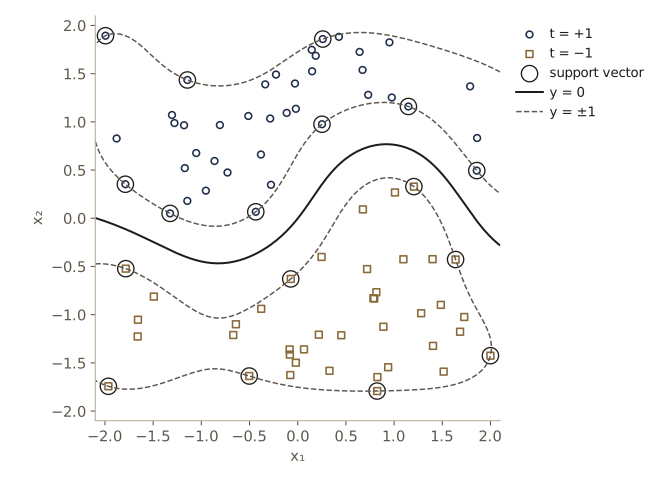
The boundary is curved in input space, but it is a hyperplane in the feature space of the Gaussian kernel, which is why the maximum-margin machinery still applies. Seventeen of the eighty points are support vectors.
Before trusting our solver further, we compare it with a general-purpose constrained optimizer from SciPy (SLSQP) on the same dual. We use SciPy only as a cross-check.
from scipy.optimize import minimize

K_wave = gaussian_kernel(X_wave, X_wave, 1.0)
Q = np.outer(t_wave, t_wave) * K_wave
dual = lambda a: a.sum() - 0.5 * a @ Q @ a           # the dual objective L~(a)
res = minimize(lambda a: -dual(a), np.zeros(80), jac=lambda a: Q @ a - 1,
               bounds=[(0, None)] * 80, method="SLSQP", options={"maxiter": 500, "ftol": 1e-12},
               constraints=[{"type": "eq", "fun": lambda a: a @ t_wave, "jac": lambda a: t_wave}])
print(f"SLSQP: converged {res.success}, dual objective {dual(res.x):.6f}")
print(f"SMO:   dual objective {dual(hard['a']):.6f}")
print(f"largest difference in any a_n: {np.abs(res.x - hard['a']).max():.1e}")
SLSQP: converged True, dual objective 9.305399
SMO:   dual objective 9.305399
largest difference in any a_n: 1.1e-06
The two solvers agree to about six digits. SLSQP works with the full \(80 \times 80\) problem at every step; an SMO iteration touches only two columns of the kernel matrix and its diagonal.
The KKT conditions make a strong prediction: the points with \(a_n = 0\) are irrelevant. If we delete them and train again, we should get exactly the same classifier. And unlike the perceptron, the order of the training data should not matter at all, because the solution of a convex problem with a unique optimum does not depend on how we find it.
grid = np.stack(np.meshgrid(np.linspace(-2, 2, 41), np.linspace(-2, 2, 41)), -1).reshape(-1, 2)
y_all = svm_decision(hard, grid)

only_sv = svm_fit(X_wave[on_margin], t_wave[on_margin], C=np.inf, gamma=1.0, tol=1e-6)
perm = rng.permutation(80)
shuffled = svm_fit(X_wave[perm], t_wave[perm], C=np.inf, gamma=1.0, tol=1e-6)
print(f"trained on the 17 support vectors only: max |change in y| on a grid = "
      f"{np.abs(svm_decision(only_sv, grid) - y_all).max():.1e}")
print(f"trained on shuffled data:               max |change in y| on a grid = "
      f"{np.abs(svm_decision(shuffled, grid) - y_all).max():.1e}")
trained on the 17 support vectors only: max |change in y| on a grid = 6.7e-07
trained on shuffled data:               max |change in y| on a grid = 8.5e-07
Note. The support vectors are the only training points that touch the solution. Any other point could be moved anywhere, as long as it stays outside the margin on its own side, without changing the classifier. This is also why an SVM can be sensitive to a few awkward points: the solution is determined by the points closest to the other class.
Why the maximum margin?
The maximum margin idea was first justified through statistical learning theory, which we sketch near the end of the SVM part of the module. There is also a probabilistic reading, due to Tong and Koller: model each class density with a kernel density estimator (module 02) using Gaussian kernels of a common width \(\sigma\), and choose the hyperplane that minimizes the probability of error under that density model. As \(\sigma \to 0\), the error is dominated by the training points closest to the boundary, and the optimal hyperplane tends to the maximum-margin one. A related picture appears in Bayesian treatments of linear classifiers: averaging over all separating hyperplanes, weighted by the posterior, tends to put the boundary near the middle of the gap between the classes.
Overlapping classes: the soft margin
Slack variables
Real classes overlap. A hard-margin SVM with a Gaussian kernel can still separate any training set of distinct points, since the kernel matrix is positive definite, but it does so by drawing an absurdly contorted boundary around each stray point. We need to allow some training points to violate the margin, at a price.
Introduce a slack variable \(\xi_n \ge 0\) for each training point, and relax the constraints to
\[t_n y(\mathbf{x}_n) \ge 1 - \xi_n, \qquad \xi_n \ge 0.\]At the optimum, \(\xi_n = \max(0, 1 - t_n y(\mathbf{x}_n))\), which sorts the points into three groups:
- \(\xi_n = 0\): on the margin boundary or beyond it, on the correct side;
- \(0 < \xi_n \le 1\): inside the margin but still correctly classified (or exactly on the boundary when \(\xi_n = 1\));
- \(\xi_n > 1\): past the decision boundary, so misclassified.
The figure of the margin geometry above shows one point from each of the last two groups. Allowing these violations turns the hard margin into a soft margin. The objective adds the total slack to the margin term:
\[\min_{\mathbf{w}, b, \boldsymbol{\xi}} \; C \sum_{n=1}^{N} \xi_n + \frac12 \lVert \mathbf{w} \rVert^2 .\]Every misclassified point has \(\xi_n > 1\), so the total slack \(\sum_n \xi_n\) can never be smaller than the number of training errors. The constant \(C > 0\) sets the exchange rate between slack and margin. A large \(C\) makes violations expensive and approaches the hard margin as \(C \to \infty\); a small \(C\) accepts many violations in return for a wide margin, a smoother boundary. So \(C\) plays the role of an inverse regularization coefficient.
Watch out. The penalty grows linearly with \(\xi_n\), not with a constant cost per mistake, so a single point far on the wrong side still pulls on the solution in proportion to how far away it is. The soft margin tolerates overlap, but it is not immune to outliers or mislabeled points.
The dual with box constraints
There are now two families of constraints, so two families of multipliers, \(a_n \ge 0\) for \(t_n y(\mathbf{x}_n) - 1 + \xi_n \ge 0\) and \(\mu_n \ge 0\) for \(\xi_n \ge 0\):
\[L = \frac12 \lVert \mathbf{w} \rVert^2 + C \sum_n \xi_n - \sum_n a_n \left\{ t_n y(\mathbf{x}_n) - 1 + \xi_n \right\} - \sum_n \mu_n \xi_n .\]The derivatives with respect to \(\mathbf{w}\) and \(b\) give the same two conditions as before, \(\mathbf{w} = \sum_n a_n t_n \boldsymbol{\phi}(\mathbf{x}_n)\) and \(\sum_n a_n t_n = 0\). The new one is
\[\frac{\partial L}{\partial \xi_n} = C - a_n - \mu_n = 0 \quad\Rightarrow\quad a_n = C - \mu_n .\]Substituting back, every term in \(\xi_n\) has coefficient \(C - a_n - \mu_n = 0\) and disappears, and what is left is exactly the same dual objective as in the separable case. The only change is in the constraints: since \(\mu_n \ge 0\), we need \(a_n \le C\).
So the soft-margin SVM dual is: maximize \(\widetilde{L}(\mathbf{a}) = \sum_n a_n - \tfrac12 \sum_n \sum_m a_n a_m t_n t_m k(\mathbf{x}_n, \mathbf{x}_m)\) subject to the box constraints \(0 \le a_n \le C\) and \(\sum_n a_n t_n = 0\).
Our smo function already handles a finite \(C\): that is what the tests against C in the index sets are for.
Reading the solution
The KKT conditions now include \(a_n \{ t_n y(\mathbf{x}_n) - 1 + \xi_n \} = 0\) and \(\mu_n \xi_n = 0\). Together with \(a_n = C - \mu_n\) they sort the training points by their multipliers:
| Multiplier | Consequence | Where the point is |
|---|---|---|
| \(a_n = 0\) | \(\mu_n = C > 0\), so \(\xi_n = 0\) and \(t_n y_n \ge 1\) | on or outside the margin, correct side; not a support vector |
| \(0 < a_n < C\) | \(\mu_n > 0\), so \(\xi_n = 0\), and \(t_n y_n = 1\) | exactly on the margin boundary |
| \(a_n = C\) | \(t_n y_n = 1 - \xi_n\) with \(\xi_n \ge 0\) | on or inside the margin; misclassified if \(\xi_n > 1\) |
The support vectors are the last two rows. Only the middle row has \(t_n y(\mathbf{x}_n) = 1\) exactly, so the bias is averaged over the set \(\mathcal{M}\) of points with \(0 < a_n < C\):
\[b = \frac{1}{N_{\mathcal{M}}} \sum_{n \in \mathcal{M}} \left( t_n - \sum_{m \in \mathcal{S}} a_m t_m k(\mathbf{x}_n, \mathbf{x}_m) \right).\]That is what smo computes at the end.
The effect of C
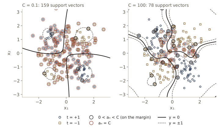
The next data set has overlapping classes: each class is a mixture of two Gaussian blobs, arranged like a noisy checkerboard. We train on 200 points and measure the error on 2,000 fresh points from the same distribution.
def make_overlap(N, seed):
    """Two overlapping classes, each an equal mixture of two Gaussian blobs (sd 0.65)."""
    g = np.random.default_rng(seed)
    t = np.where(g.random(N) < 0.5, 1.0, -1.0)
    comp = g.integers(0, 2, N)
    centers = {1.0: np.array([[-1.0, 0.9], [1.0, -0.9]]),
               -1.0: np.array([[1.0, 0.9], [-1.0, -0.9]])}
    mu = np.array([centers[tn][c] for tn, c in zip(t, comp)])
    return mu + 0.65 * g.standard_normal((N, 2)), t

X_tr, t_tr = make_overlap(200, seed=11)
X_te, t_te = make_overlap(2000, seed=12)
error_rate = lambda model, X, t: np.mean(np.sign(svm_decision(model, X)) != t)

print("     C   SVs  a_n = C  train err  test err  SMO iters")
for C in [0.1, 1.0, 10.0, 100.0, 1000.0]:
    m = svm_fit(X_tr, t_tr, C=C, gamma=0.5)
    at_C = (m["a"] > C - 1e-8).sum()
    print(f"{C:6g}  {len(m['at']):4d}  {at_C:7d}  {error_rate(m, X_tr, t_tr):9.3f}"
          f"  {error_rate(m, X_te, t_te):8.3f}  {m['iters']:9d}")
     C   SVs  a_n = C  train err  test err  SMO iters
   0.1   159      153      0.160     0.141         88
     1   101       87      0.150     0.143        113
    10    84       66      0.150     0.153        358
   100    78       55      0.130     0.165       2964
  1000    78       51      0.125     0.178      12735
Read the table from top to bottom. With \(C = 0.1\) the margin is wide, most points are inside it, and 159 of the 200 points are support vectors, almost all of them with \(a_n = C\). As \(C\) grows, the margin narrows, fewer points are inside it, the number of support vectors falls, and the training error drops from 0.160 to 0.125. The test error moves the other way: it is lowest for the two smallest values of \(C\) (0.141 and 0.143) and climbs to 0.178 at \(C = 1000\), the usual sign of overfitting. The optimizer also works harder for large \(C\), because the problem becomes more poorly conditioned. As with any regularization constant, \(C\) (and the kernel width \(\gamma\)) is normally chosen by cross-validation.
The ν-SVM
The constant \(C\) has no direct interpretation, which makes it hard to guess a good value. The ν-SVM of Schölkopf and colleagues replaces it with a parameter \(\nu \in (0, 1]\) that has one. Its dual maximizes
\[\widetilde{L}(\mathbf{a}) = -\frac12 \sum_n \sum_m a_n a_m t_n t_m k(\mathbf{x}_n, \mathbf{x}_m)\]subject to \(0 \le a_n \le 1/N\), \(\sum_n a_n t_n = 0\), and \(\sum_n a_n \ge \nu\). It can be shown that at most a fraction \(\nu\) of the training points end up as margin errors (points with \(\xi_n > 0\), which lie inside the margin or beyond it), and at least a fraction \(\nu\) end up as support vectors. So setting \(\nu = 0.2\) says, roughly, “let about a fifth of the training points violate the margin”. The two formulations trace out the same family of classifiers; they differ only in how the family is parametrized. The extra inequality constraint means our two-variable SMO step would need modification, so we do not implement it here.
Solving the QP at scale
Training uses all \(N\) points even though prediction uses only the support vectors, so the cost of the quadratic program matters. Storing the kernel matrix alone takes \(N^2\) numbers. Three families of methods have been used, in order of increasing aggressiveness:
- Chunking uses the fact that rows and columns of the kernel matrix belonging to multipliers that are zero can be removed without changing the objective. It solves a sequence of smaller QPs that together identify the nonzero multipliers, so the matrix it handles has roughly the size of the support set.
- Decomposition methods also solve a sequence of small QPs, but of a fixed size, so they scale to arbitrarily large data sets; each subproblem still needs a numerical QP solver.
- SMO is decomposition with working sets of size two, solved in closed form as above. In practice its running time grows somewhere between linearly and quadratically with \(N\), depending on the problem. Practical implementations cache kernel columns rather than storing the whole matrix; our version keeps the whole matrix for clarity.
Kernels do not escape the curse of dimensionality
Since the kernel lets us work in feature spaces of huge or infinite dimension, it might seem that SVMs are immune to the curse of dimensionality of module 01. They are not, because the feature vectors are highly constrained. Take the second-order polynomial kernel \(k(\mathbf{x}, \mathbf{z}) = (1 + \mathbf{x}^{\mathrm{T}} \mathbf{z})^2\) in two dimensions. Expanding the square shows that it is an inner product of six-dimensional feature vectors
\[\boldsymbol{\phi}(\mathbf{x}) = \left( 1, \sqrt{2} x_1, \sqrt{2} x_2, x_1^2, \sqrt{2} x_1 x_2, x_2^2 \right)^{\mathrm{T}},\]but these six features are fixed functions of just two numbers. All inputs map onto a two-dimensional curved surface inside the six-dimensional space; the effective dimensionality is still two.
def phi_poly2(x):
    """Explicit feature map of k(x, z) = (1 + x^T z)^2 for 2-D inputs."""
    x1, x2 = x
    r2 = np.sqrt(2)
    return np.array([1, r2 * x1, r2 * x2, x1 ** 2, r2 * x1 * x2, x2 ** 2])

x, zz = rng.standard_normal(2), rng.standard_normal(2)
print(f"kernel (1 + x.z)^2 = {(1 + x @ zz) ** 2:.6f}   phi(x).phi(z) = {phi_poly2(x) @ phi_poly2(zz):.6f}")
kernel (1 + x.z)^2 = 1.016226 phi(x).phi(z) = 1.016226
Probabilities from an SVM
The SVM is a decision machine: it outputs a class, or a score \(y(\mathbf{x})\), not a probability. That is a limitation whenever the output feeds into a larger system, or into the decision theory of module 01 with unequal costs. A common fix, proposed by Platt, fits a logistic sigmoid to the scores after training,
\[p(t = 1 \mid \mathbf{x}) = \sigma\left( A\, y(\mathbf{x}) + B \right),\]choosing \(A\) and \(B\) by minimizing the cross-entropy on a separate labeled set (fitting them on the SVM’s own training data overfits badly, since the training points were pushed out to the margins on purpose). This amounts to assuming that \(y(\mathbf{x})\) is proportional to the log-odds, which nothing in SVM training encourages, so the resulting probabilities can be poor. With two parameters, Newton’s method (as in the IRLS algorithm of module 04) converges in a few steps.
def platt_fit(f, t, iters=50):
    """Fit p(t=1 | f) = sigmoid(A f + B) by Newton's method on the cross-entropy."""
    A, B = 1.0, 0.0
    y = (t > 0).astype(float)
    F = np.c_[f, np.ones_like(f)]                    # "design matrix" for (A, B)
    for _ in range(iters):
        p = expit(A * f + B)
        grad = F.T @ (p - y)
        H = F.T @ (F * (p * (1 - p))[:, None])
        step = np.linalg.solve(H, grad)
        A, B = A - step[0], B - step[1]
        if np.abs(step).max() < 1e-10:
            break
    return A, B

svm1 = svm_fit(X_tr, t_tr, C=1.0, gamma=0.5)
X_val, t_val = make_overlap(300, seed=13)             # held-out set for A and B
A, B = platt_fit(svm_decision(svm1, X_val), t_val)
p_te = expit(A * svm_decision(svm1, X_te) + B)
print(f"A = {A:.3f}, B = {B:.3f}")
print("predicted p    mean p   observed frequency   count")
for lo, hi in [(0, .2), (.2, .4), (.4, .6), (.6, .8), (.8, 1)]:
    sel = (p_te >= lo) & (p_te < hi)
    print(f"[{lo:.1f}, {hi:.1f})    {p_te[sel].mean():.3f}   {np.mean(t_te[sel] > 0):17.3f}   {sel.sum():5d}")
A = 2.238, B = -0.048
predicted p    mean p   observed frequency   count
[0.0, 0.2)    0.065               0.081     791
[0.2, 0.4)    0.299               0.357     182
[0.4, 0.6)    0.503               0.513     189
[0.6, 0.8)    0.718               0.742     190
[0.8, 1.0)    0.920               0.957     648
On this problem the calibrated probabilities follow the observed class frequencies reasonably well; the largest discrepancy, about 0.06, is in the \([0.2, 0.4)\) bin. That is a good outcome, not a guaranteed one.
Relation to logistic regression
The soft-margin SVM can be written as an unconstrained regularized error, which makes the comparison with logistic regression direct. At the optimum each slack variable takes its smallest allowed value, \(\xi_n = \max(0, 1 - t_n y_n)\) with \(y_n = y(\mathbf{x}_n)\). Substituting into the objective and dividing by \(C\):
\[\sum_{n=1}^{N} E_{\text{SV}}(y_n t_n) + \lambda \lVert \mathbf{w} \rVert^2, \qquad E_{\text{SV}}(z) = \left[ 1 - z \right]_+, \qquad \lambda = \frac{1}{2C},\]where \([u]_+ = \max(0, u)\) is the positive part. \(E_{\text{SV}}\) is the hinge loss, named for its shape: zero for \(z \ge 1\), then a straight line.
Now logistic regression, rewritten for targets in \(\{-1, +1\}\). With \(p(t = 1 \mid y) = \sigma(y)\) and the symmetry \(1 - \sigma(y) = \sigma(-y)\), both cases are covered by \(p(t \mid y) = \sigma(y t)\). The negative log-likelihood of one point is then \(-\ln \sigma(y t) = \ln(1 + e^{-y t})\), and with a quadratic regularizer the objective is
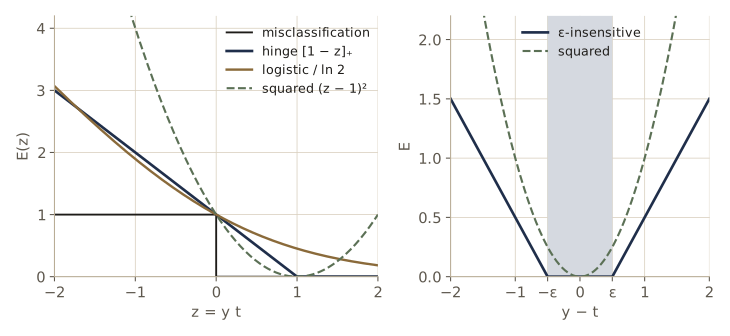
\[\sum_{n=1}^{N} E_{\text{LR}}(y_n t_n) + \lambda \lVert \mathbf{w} \rVert^2, \qquad E_{\text{LR}}(z) = \ln\left( 1 + e^{-z} \right).\]The two objectives have the same structure and differ only in the loss applied to \(z = y t\). Dividing \(E_{\text{LR}}\) by \(\ln 2\) makes it pass through \((0, 1)\), like the hinge loss, and the figure below compares them with two other losses.
What to notice:
- Both are convex stand-ins for the misclassification error, the 0–1 step we would really like to minimize but cannot, because it is flat almost everywhere and not convex. Both upper-bound the step (after rescaling the logistic loss), and both grow linearly for badly misclassified points.
- The hinge loss has a flat part. Points with \(t_n y_n > 1\) contribute nothing to the objective or to its gradient, which is exactly why their multipliers are zero and the solution is sparse. The logistic loss is positive everywhere, so every point pulls on the solution a little, and kernelized logistic regression has no sparsity.
- The logistic loss gives probabilities; the hinge loss does not.
- The squared error is a poor classification loss. Written as \((y - t)^2 = (1 - yt)^2\) for \(t = \pm 1\), it penalizes points that are classified correctly with a large score (\(z \gg 1\)), so those points drag the boundary toward themselves and away from the difficult region. A loss that never increases with \(z\) is the right shape for classification. This is the failure of least-squares classification we saw in module 04.
Since the primal of this section and the dual solved by SMO are the same problem, their optimal values must agree. The primal value of the hinge form can be computed from the dual solution, because \(\lVert \mathbf{w} \rVert^2 = \mathbf{a}^{\mathrm{T}} \mathbf{Q} \mathbf{a}\), and the duality gap between the two values is a certificate of how close to optimal the solver got.
K_tr = gaussian_kernel(X_tr, X_tr, 0.5)
Q_tr = np.outer(t_tr, t_tr) * K_tr
a1 = svm1["a"]
ty1 = t_tr * svm_decision(svm1, X_tr)
w_sq = a1 @ Q_tr @ a1                                         # ||w||^2
primal = 1.0 * np.maximum(0, 1 - ty1).sum() + 0.5 * w_sq      # C sum_n xi_n + ||w||^2 / 2, C = 1
dual_value = a1.sum() - 0.5 * w_sq
print(f"primal (hinge form) = {primal:.4f}   dual = {dual_value:.4f}   gap = {primal - dual_value:.1e}")
print("points with t_n y_n > 1 (flat part of the hinge):", (ty1 > 1 + 1e-3).sum(),
      "  of which have a_n = 0:", ((ty1 > 1 + 1e-3) & (a1 < 1e-8)).sum())
primal (hinge form) = 82.8882   dual = 82.8869   gap = 1.3e-03
points with t_n y_n > 1 (flat part of the hinge): 99   of which have a_n = 0: 99
The gap is a tiny fraction of the objective, so the SMO solution is essentially optimal for the hinge-loss problem as well. And every point on the flat part of the hinge has a zero multiplier, as the KKT analysis predicts.
Multiclass SVMs
The SVM is a two-class machine, and there is no single agreed way to extend it to \(K > 2\) classes. The common options each have a flaw.
One-versus-the-rest. Train \(K\) classifiers; classifier \(k\) treats class \(\mathcal{C}_k\) as positive and all other classes as negative. As module 04 showed for linear discriminants, the signs of the \(K\) outputs can be inconsistent: a point may be claimed by several classifiers, or by none. The usual repair is to predict \(\arg\max_k y_k(\mathbf{x})\), but the \(K\) classifiers were trained on different problems, so nothing guarantees that their outputs are on comparable scales. The training sets are also unbalanced: with ten equally frequent classes, each classifier sees 10% positives and 90% negatives. (Variants adjust the targets, for instance to \(+1\) and \(-1/(K-1)\), to restore some symmetry.)
One-versus-one. Train \(K(K - 1)/2\) classifiers, one per pair of classes, and let them vote. Votes can tie, and the number of classifiers grows quadratically, although each is trained on only two classes’ data. Arranging the pairwise classifiers in a directed acyclic graph (the DAGSVM) reduces the work at test time to \(K - 1\) evaluations.
Other schemes. One can also train all \(K\) classifiers jointly with a single objective that asks each class’s output to beat the others by a margin; this is more principled but costs about \(O(K^2 N^2)\) instead of \(O(K N^2)\). Error-correcting output codes train classifiers on more general splits of the classes into two groups and decode the pattern of their outputs, which adds robustness to individual mistakes. In practice one-versus-the-rest remains the most common choice, despite its ad hoc nature.
Here are the first two on three overlapping Gaussian classes, reusing svm_fit:
def make_three(N, seed):
    """Three overlapping Gaussian classes in 2-D (labels 0, 1, 2)."""
    g = np.random.default_rng(seed)
    k = g.integers(0, 3, N)
    centers = np.array([[0.0, 1.2], [-1.2, -0.8], [1.2, -0.8]])
    return centers[k] + 0.8 * g.standard_normal((N, 2)), k

X3, k3 = make_three(150, seed=21)
X3_te, k3_te = make_three(3000, seed=22)

# one-versus-the-rest: K classifiers
Y = np.column_stack([svm_decision(svm_fit(X3, np.where(k3 == c, 1.0, -1.0), C=1.0, gamma=0.5), X3_te)
                     for c in range(3)])
claims = (Y > 0).sum(1)
print(f"one-vs-rest: fraction of test points claimed by no classifier {np.mean(claims == 0):.3f},"
      f" by one {np.mean(claims == 1):.3f}, by two or more {np.mean(claims >= 2):.3f}")
print(f"one-vs-rest: accuracy of argmax_k y_k = {np.mean(Y.argmax(1) == k3_te):.3f} overall,"
      f" {np.mean(Y.argmax(1)[claims == 0] == k3_te[claims == 0]):.3f} on the unclaimed points")

# one-versus-one: K(K-1)/2 classifiers, majority vote
votes = np.zeros((len(X3_te), 3), dtype=int)
for c1, c2 in [(0, 1), (0, 2), (1, 2)]:
    pair = (k3 == c1) | (k3 == c2)
    m = svm_fit(X3[pair], np.where(k3[pair] == c1, 1.0, -1.0), C=1.0, gamma=0.5)
    winner = np.where(svm_decision(m, X3_te) > 0, c1, c2)
    votes[np.arange(len(X3_te)), winner] += 1
tied = votes.max(1) == 1                                        # a 1-1-1 cycle
print(f"one-vs-one:  three-way ties on {tied.sum()} of {len(tied)} test points;"
      f" accuracy where not tied = {np.mean(votes.argmax(1)[~tied] == k3_te[~tied]):.3f}")
one-vs-rest: fraction of test points claimed by no classifier 0.033, by one 0.967, by two or more 0.000
one-vs-rest: accuracy of argmax_k y_k = 0.882 overall, 0.551 on the unclaimed points
one-vs-one:  three-way ties on 0 of 3000 test points; accuracy where not tied = 0.881
With one-versus-the-rest, about 3% of the test points are claimed by no classifier, and the argmax rule has to settle them. It does so poorly: on those points it is right only about 55% of the time, against 88% overall, because it compares outputs of three differently trained machines. On this data set no point is claimed twice and the one-versus-one vote never ends in a three-way tie; such ties can only happen in the small region where the three pairwise boundaries disagree in a cycle, and with well-separated centers that region is tiny. The overall accuracies of the two schemes are almost the same. The RVM, later in the module, handles \(K\) classes with a single probabilistic model instead.
One-class SVMs. A related unsupervised use of the same machinery finds a boundary around the region where most of the data lie, without estimating a full density: for example, the smallest ball in feature space that encloses the data apart from a fraction \(\nu\) of outlying points, or the maximum-margin hyperplane that puts the origin on one side and the data, again apart from a fraction \(\nu\), on the other. For kernels that depend only on \(\mathbf{x} - \mathbf{x}'\), the two formulations coincide. Such novelty detectors flag test points that fall outside the boundary.
SVMs for regression
The ε-insensitive error
To carry sparsity over to regression, we replace the squared error of regularized least squares, \(\tfrac12 \sum_n (y_n - t_n)^2 + \tfrac{\lambda}{2} \lVert \mathbf{w} \rVert^2\), with an error that ignores small residuals. The ε-insensitive error is
\[E_\epsilon\left( y(\mathbf{x}) - t \right) = \begin{cases} 0, & \text{if } \lvert y(\mathbf{x}) - t \rvert < \epsilon, \\ \lvert y(\mathbf{x}) - t \rvert - \epsilon, & \text{otherwise}, \end{cases}\]shown in the right panel of the loss figure. Targets within a tube of half-width \(\epsilon\) around the prediction cost nothing, just as points beyond the margin cost nothing in classification. We minimize
\[C \sum_{n=1}^{N} E_\epsilon\left( y(\mathbf{x}_n) - t_n \right) + \frac12 \lVert \mathbf{w} \rVert^2,\]with \(y(\mathbf{x}) = \mathbf{w}^{\mathrm{T}} \boldsymbol{\phi}(\mathbf{x}) + b\) and, by convention, the constant \(C\) in front of the error term.
Slack variables and the dual
A target can now miss the tube on either side, so each point gets two slack variables: \(\xi_n \ge 0\) for targets above the tube and \(\widehat{\xi}_n \ge 0\) for targets below it. The problem becomes
\[\begin{aligned} \min_{\mathbf{w}, b, \boldsymbol{\xi}, \widehat{\boldsymbol{\xi}}} \quad & C \sum_n \left( \xi_n + \widehat{\xi}_n \right) + \frac12 \lVert \mathbf{w} \rVert^2 \\ \text{subject to} \quad & t_n \le y_n + \epsilon + \xi_n, \quad t_n \ge y_n - \epsilon - \widehat{\xi}_n, \quad \xi_n \ge 0, \quad \widehat{\xi}_n \ge 0 . \end{aligned}\]With multipliers \(a_n, \widehat{a}_n \ge 0\) for the two tube constraints and \(\mu_n, \widehat{\mu}_n \ge 0\) for the slack constraints, the Lagrangian is
\[\begin{aligned} L = {} & C \sum_n (\xi_n + \widehat{\xi}_n) + \frac12 \lVert \mathbf{w} \rVert^2 - \sum_n (\mu_n \xi_n + \widehat{\mu}_n \widehat{\xi}_n) \\ & - \sum_n a_n (\epsilon + \xi_n + y_n - t_n) - \sum_n \widehat{a}_n (\epsilon + \widehat{\xi}_n - y_n + t_n). \end{aligned}\]Setting the derivatives with respect to \(\mathbf{w}\), \(b\), \(\xi_n\), and \(\widehat{\xi}_n\) to zero gives
\[\begin{aligned} & \mathbf{w} = \sum_n (a_n - \widehat{a}_n) \boldsymbol{\phi}(\mathbf{x}_n), \qquad \sum_n (a_n - \widehat{a}_n) = 0, \\ & a_n + \mu_n = C, \qquad \widehat{a}_n + \widehat{\mu}_n = C . \end{aligned}\]Substituting back, the slack terms cancel as in classification, and the result is the dual.
\[\begin{aligned} \widetilde{L}(\mathbf{a}, \widehat{\mathbf{a}}) = {} & -\frac12 \sum_n \sum_m (a_n - \widehat{a}_n)(a_m - \widehat{a}_m) k(\mathbf{x}_n, \mathbf{x}_m) \\ & - \epsilon \sum_n (a_n + \widehat{a}_n) + \sum_n (a_n - \widehat{a}_n) t_n . \end{aligned}\]Support vector regression maximizes the dual \(\widetilde{L}(\mathbf{a}, \widehat{\mathbf{a}})\) above subject to \(0 \le a_n \le C\), \(0 \le \widehat{a}_n \le C\), and \(\sum_n (a_n - \widehat{a}_n) = 0\). Predictions use \(y(\mathbf{x}) = \sum_n (a_n - \widehat{a}_n) k(\mathbf{x}, \mathbf{x}_n) + b\).
The KKT complementary slackness conditions are
\[\begin{aligned} a_n (\epsilon + \xi_n + y_n - t_n) &= 0, & \widehat{a}_n (\epsilon + \widehat{\xi}_n - y_n + t_n) &= 0, \\ (C - a_n) \xi_n &= 0, & (C - \widehat{a}_n) \widehat{\xi}_n &= 0 . \end{aligned}\]So \(a_n > 0\) only if \(t_n = y_n + \epsilon + \xi_n\), meaning the target is on the upper edge of the tube or above it, and \(\widehat{a}_n > 0\) only if the target is on the lower edge or below it. Both cannot happen at once: adding the two equations would give \(2\epsilon + \xi_n + \widehat{\xi}_n = 0\), impossible with \(\epsilon > 0\). Every target strictly inside the tube has \(a_n = \widehat{a}_n = 0\) and drops out of the prediction. The support vectors are the points on the edges of the tube or outside it. For the bias, a point with \(0 < a_n < C\) has \(\xi_n = 0\) and so sits exactly on the upper edge, \(t_n = y_n + \epsilon\), which gives \(b = t_n - \epsilon - \sum_m (a_m - \widehat{a}_m) k(\mathbf{x}_n, \mathbf{x}_m)\); points with \(0 < \widehat{a}_n < C\) give an analogous formula, and in practice one averages all of them.
Solving it with the same SMO
Stack the variables as \(\boldsymbol{\beta} = (\mathbf{a}, \widehat{\mathbf{a}})\), a vector of length \(2N\), with \(\mathbf{z} = (\mathbf{1}, -\mathbf{1})\). Then \(\sum_n z_n \beta_n = \sum_n (a_n - \widehat{a}_n)\), the equality constraint. The quadratic term \((\mathbf{a} - \widehat{\mathbf{a}})^{\mathrm{T}} \mathbf{K} (\mathbf{a} - \widehat{\mathbf{a}})\) equals \(\boldsymbol{\beta}^{\mathrm{T}} \mathbf{Q} \boldsymbol{\beta}\) with \(Q_{nm} = z_n z_m \widetilde{K}_{nm}\) and \(\widetilde{\mathbf{K}} = \begin{pmatrix} \mathbf{K} & \mathbf{K} \\ \mathbf{K} & \mathbf{K} \end{pmatrix}\), and minimizing \(-\widetilde{L}\) gives the linear term \(\mathbf{p} = (\epsilon \mathbf{1} - \mathbf{t}, \; \epsilon \mathbf{1} + \mathbf{t})\). That is exactly the form smo solves, and its bias comes out right too: for a free \(a_n\), \(v_n = t_n - \epsilon - \sum_m (a_m - \widehat{a}_m) k(\mathbf{x}_n, \mathbf{x}_m)\), the formula above.
Our regression data set is the course’s running example: \(N = 50\) inputs drawn uniformly on \([0, 1]\), targets \(\sin(2\pi x) +\) Gaussian noise with standard deviation 0.2. We use a Gaussian kernel with \(\gamma = 20\) (width \(\sigma = 1/\sqrt{2\gamma} \approx 0.16\)).
def make_sin(N, sd, seed):
    """x ~ U(0, 1) (sorted), t = sin(2 pi x) + Gaussian noise with standard deviation sd."""
    g = np.random.default_rng(seed)
    x = np.sort(g.uniform(0, 1, N))
    return x, np.sin(2 * np.pi * x) + sd * g.standard_normal(N)

def svr_fit(X, t, C, eps, gamma, tol=1e-3):
    """epsilon-SVR with a Gaussian kernel, via SMO on the stacked variables (a, a_hat)."""
    N = len(t)
    K = gaussian_kernel(X, X, gamma)
    Kt = np.block([[K, K], [K, K]])
    z = np.r_[np.ones(N), -np.ones(N)]
    p = np.r_[eps - t, eps + t]
    beta, b, iters = smo(Kt, z, p, C, tol)
    a, a_hat = beta[:N], beta[N:]
    return {"X": X, "coef": a - a_hat, "a": a, "a_hat": a_hat, "b": b, "gamma": gamma,
            "sv": (a > 1e-8) | (a_hat > 1e-8), "iters": iters}

def svr_predict(model, Xnew):
    return gaussian_kernel(Xnew, model["X"], model["gamma"]) @ model["coef"] + model["b"]

x_sin, t_sin = make_sin(50, sd=0.2, seed=5)
X_sin = x_sin[:, None]
x_grid = np.linspace(0, 1, 201)[:, None]
truth = np.sin(2 * np.pi * x_grid[:, 0])

print(" eps     C   SVs  outside tube  both a, a_hat > 0  rms error vs sin(2 pi x)")
for eps, C in [(0.1, 1.0), (0.2, 1.0), (0.2, 10.0), (0.3, 1.0)]:
    svr = svr_fit(X_sin, t_sin, C, eps, gamma=20.0)
    resid = np.abs(svr_predict(svr, X_sin) - t_sin)
    rms = np.sqrt(np.mean((svr_predict(svr, x_grid) - truth) ** 2))
    both = ((svr["a"] > 1e-8) & (svr["a_hat"] > 1e-8)).sum()
    print(f"{eps:4.1f}  {C:4g}  {svr['sv'].sum():4d}  {(resid > eps + 1e-3).sum():12d}"
          f"  {both:17d}  {rms:24.3f}")
 eps     C   SVs  outside tube  both a, a_hat > 0  rms error vs sin(2 pi x)
 0.1     1    28            21                  0                     0.097
 0.2     1    15             8                  0                     0.078
 0.2    10    16             9                  0                     0.111
 0.3     1     7             1                  0                     0.103
Every row obeys the KKT analysis: no point has both multipliers nonzero, and the support vectors are the points outside the tube plus a few exactly on its edges. The tube width controls sparsity directly. With \(\epsilon = 0.1\), half the noise standard deviation, 21 of the 50 targets fall outside the tube and 28 points are support vectors; with \(\epsilon = 0.3\) only 7 are. In all four settings the fitted curve is close to the true function; we will compare the \(\epsilon = 0.2\), \(C = 1\) fit with the RVM below.
ν-SVR. As in classification, there is a ν-formulation of regression that fixes a parameter \(\nu\) instead of the tube width. It maximizes \(-\tfrac12 \sum_n \sum_m (a_n - \widehat{a}_n)(a_m - \widehat{a}_m) k(\mathbf{x}_n, \mathbf{x}_m) + \sum_n (a_n - \widehat{a}_n) t_n\) subject to \(0 \le a_n, \widehat{a}_n \le C/N\), \(\sum_n (a_n - \widehat{a}_n) = 0\), and \(\sum_n (a_n + \widehat{a}_n) \le \nu C\). The width \(\epsilon\) is then found as part of the solution, and at most a fraction \(\nu\) of the points lie outside the tube while at least a fraction \(\nu\) are support vectors.
Computational learning theory
SVMs grew out of computational learning theory (also called statistical learning theory), which asks how much data is needed before a learning algorithm can be trusted to generalize. We give the two central ideas and one worked bound.
PAC learning
The setting: data \((\mathbf{x}, t)\) come from an unknown distribution \(p(\mathbf{x}, t)\), and, in the simplest version, labels are a deterministic function \(t = g(\mathbf{x})\) of the input. A learning algorithm picks a function \(f(\mathbf{x}; \mathcal{D})\) from a class \(\mathcal{F}\) using a training set \(\mathcal{D}\) of \(N\) independent samples. Its true error rate \(\mathbb{E}_{\mathbf{x}, t}[\mathrm{I}(f(\mathbf{x}; \mathcal{D}) \neq t)]\), where \(\mathrm{I}\) is the indicator function, is itself random, because \(\mathcal{D}\) is. We call learning probably approximately correct (PAC) if, with probability at least \(1 - \delta\) over the draw of \(\mathcal{D}\), the error is below \(\epsilon\). The question is how large \(N\) must be, given \(\epsilon\) and \(\delta\). The framework is due to Valiant.
Here is the simplest bound, for a finite class \(\mathcal{F}\) and an algorithm that returns any function consistent with the training data. Call a function bad if its true error exceeds \(\epsilon\). A bad function agrees with one random example with probability less than \(1 - \epsilon\), so it agrees with all \(N\) with probability less than \((1 - \epsilon)^N \le e^{-\epsilon N}\). By the union bound, the probability that any bad function in \(\mathcal{F}\) survives is less than \(\lvert \mathcal{F} \rvert e^{-\epsilon N}\). Requiring this to be at most \(\delta\) gives
\[N \ge \frac{1}{\epsilon} \left( \ln \lvert \mathcal{F} \rvert + \ln \frac{1}{\delta} \right).\]The size of the class enters only through its logarithm, a measure of how many bits it takes to name a function in it.
The VC dimension
Most useful classes are infinite: there are infinitely many lines in the plane. The Vapnik–Chervonenkis (VC) dimension replaces \(\ln \lvert \mathcal{F} \rvert\) by a combinatorial measure of richness. A set of points is shattered by \(\mathcal{F}\) if every one of the \(2^n\) ways of labeling the points can be realized by some function in \(\mathcal{F}\). The VC dimension of \(\mathcal{F}\) is the size of the largest set it can shatter.
For linear classifiers in the plane, three points in general position can be shattered, but no four points can (a classical argument, Radon’s theorem, shows that any four points can be split into two groups whose convex hulls intersect, and that labeling cannot be separated). So the VC dimension is 3; in \(D\) dimensions it is \(D + 1\). We can test shattering with our own linear SVM, using a large \(C\) and checking for zero training error.
def separable(X, t, C=1e3):
    """Can a line separate the labeled points? (soft-margin linear SVM, large C, zero error)"""
    a, b, _ = smo(X @ X.T, t, -np.ones(len(t)), C)
    return np.all(t * (X @ ((a * t) @ X) + b) > 0)

def shattered(X):
    """True if every labeling of the rows of X can be produced by a line."""
    for labels in product([-1.0, 1.0], repeat=len(X)):
        t = np.array(labels)
        if abs(t.sum()) == len(t):
            continue                         # one class only: put the line far away
        if not separable(X, t):
            return False
    return True

print("3 points (a triangle):", shattered(np.array([[0., 0.], [1., 0.], [0., 1.]])))
print("4 points (a square):  ", shattered(np.array([[0., 0.], [1., 0.], [0., 1.], [1., 1.]])))
print("random 4-point sets shattered:", sum(shattered(rng.standard_normal((4, 2))) for _ in range(25)), "of 25")
3 points (a triangle): True
4 points (a square):   False
random 4-point sets shattered: 0 of 25
The square fails on the XOR labeling, and none of the random four-point sets can be shattered either. VC theory then gives bounds that hold for every distribution. One classic form (see Burges’s tutorial in “Going further”) says that with probability at least \(1 - \delta\), for every \(f\) in a class of VC dimension \(h\),
\[\text{true error} \le \text{training error} + \sqrt{\frac{h \left( \ln(2N/h) + 1 \right) + \ln(4/\delta)}{N}} .\]def pac_sample_size(n_functions, eps, delta):
return math.ceil((math.log(n_functions) + math.log(1 / delta)) / eps)
def vc_gap(h, N, delta):
return math.sqrt((h * (math.log(2 * N / h) + 1) + math.log(4 / delta)) / N)
print("finite class, 2^20 functions, eps = 0.05, delta = 0.01: N >=", pac_sample_size(2 ** 20, 0.05, 0.01))
for N in [1_000, 10_000, 100_000]:
print(f"VC bound, h = 50, delta = 0.05, N = {N:>7,}: true error <= training error + {vc_gap(50, N, 0.05):.3f}")
finite class, 2^20 functions, eps = 0.05, delta = 0.01: N >= 370
VC bound, h = 50, delta = 0.05, N =   1,000: true error <= training error + 0.489
VC bound, h = 50, delta = 0.05, N =  10,000: true error <= training error + 0.188
VC bound, h = 50, delta = 0.05, N = 100,000: true error <= training error + 0.068
The bounds hold for any distribution and any function in the class, which is both their strength and their weakness. Real problems have far more structure than the worst case (neighboring inputs usually share a label), so the bounds are very pessimistic: ten thousand points and a modest VC dimension still only guarantee that the true error is within about 0.2 of the training error. They have had little direct practical use. Their influence has been conceptual: bounds of this type depend on the margin relative to the spread of the data rather than on the dimension of the feature space, which is the theoretical motivation for maximizing the margin. The PAC-Bayesian framework tightens the bounds by placing a distribution over \(\mathcal{F}\), somewhat like a prior, but it still covers every possible \(p(\mathbf{x}, t)\) and remains conservative.
Relevance vector machines
What the SVM leaves unsolved
The SVM works well, but by now we have met its limitations:
- its outputs are decisions, not probabilities (Platt scaling is an afterthought);
- it is inherently a two-class method;
- the constants \(C\) (or \(\nu\)) and, for regression, \(\epsilon\) must be set by cross-validation, which means training many times;
- predictions are combinations of kernels centered on training points, and the kernel must be positive semidefinite.
The relevance vector machine (RVM), introduced by Tipping, is a Bayesian sparse kernel method that removes these limitations while keeping the SVM’s form of prediction. It usually ends up much sparser than the SVM, too.
The RVM for regression
The RVM for regression is the Bayesian linear model of module 03,
\[p(t \mid \mathbf{x}, \mathbf{w}, \beta) = \mathcal{N}\left( t \mid y(\mathbf{x}), \beta^{-1} \right), \qquad y(\mathbf{x}) = \sum_{i=1}^{M} w_i \phi_i(\mathbf{x}) = \mathbf{w}^{\mathrm{T}} \boldsymbol{\phi}(\mathbf{x}),\]with noise precision \(\beta\). To mirror the SVM, the basis functions are a constant (for the bias) and one kernel centered on each training point, \(y(\mathbf{x}) = \sum_{n=1}^{N} w_n k(\mathbf{x}, \mathbf{x}_n) + b\), so \(M = N + 1\). But nothing below depends on that choice: the kernel need not be positive semidefinite, and the basis functions need not sit on data points.
The one new ingredient is the prior. Module 03 used a single precision \(\alpha\) shared by all weights. The RVM gives each weight its own:
\[p(\mathbf{w} \mid \boldsymbol{\alpha}) = \prod_{i=1}^{M} \mathcal{N}\left( w_i \mid 0, \alpha_i^{-1} \right).\]When we maximize the evidence over all the \(\alpha_i\), many of them go to infinity. A weight whose prior precision is infinite is pinned at zero, and its basis function disappears from the model. This mechanism is called automatic relevance determination (ARD), and the training points whose kernels survive are the relevance vectors.
The posterior. For fixed hyperparameters this is ordinary Bayesian linear regression with prior covariance \(\mathbf{A}^{-1}\), \(\mathbf{A} = \operatorname{diag}(\alpha_i)\). Completing the square as in module 03, the posterior is Gaussian, \(p(\mathbf{w} \mid \mathbf{t}, \mathbf{X}, \boldsymbol{\alpha}, \beta) = \mathcal{N}(\mathbf{w} \mid \mathbf{m}, \boldsymbol{\Sigma})\), with
\[\boldsymbol{\Sigma} = \left( \mathbf{A} + \beta \mathbf{\Phi}^{\mathrm{T}} \mathbf{\Phi} \right)^{-1}, \qquad \mathbf{m} = \beta \boldsymbol{\Sigma} \mathbf{\Phi}^{\mathrm{T}} \mathbf{t},\]where \(\mathbf{\Phi}\) is the \(N \times M\) design matrix, \(\Phi_{ni} = \phi_i(\mathbf{x}_n)\).
The evidence. Integrating out \(\mathbf{w}\) (a linear-Gaussian model, module 02) gives the marginal likelihood
\[\begin{aligned} \ln p(\mathbf{t} \mid \mathbf{X}, \boldsymbol{\alpha}, \beta) &= \ln \mathcal{N}(\mathbf{t} \mid \mathbf{0}, \mathbf{C}) = -\frac12 \left\{ N \ln(2\pi) + \ln \lvert \mathbf{C} \rvert + \mathbf{t}^{\mathrm{T}} \mathbf{C}^{-1} \mathbf{t} \right\}, \\ \mathbf{C} &= \beta^{-1} \mathbf{I} + \mathbf{\Phi} \mathbf{A}^{-1} \mathbf{\Phi}^{\mathrm{T}} . \end{aligned}\]This is a Gaussian process (module 06) whose covariance is a sum of rank-one terms, one per basis function: \(\mathbf{C} = \beta^{-1} \mathbf{I} + \sum_i \alpha_i^{-1} \boldsymbol{\varphi}_i \boldsymbol{\varphi}_i^{\mathrm{T}}\), where \(\boldsymbol{\varphi}_i\) is the \(i\)th column of \(\mathbf{\Phi}\), the values of basis function \(i\) at all \(N\) inputs. Setting \(\alpha_i = \infty\) removes a term.
Re-estimation equations. As in the evidence approximation of module 03, we write the evidence in terms of the posterior:
\[\begin{aligned} \ln p(\mathbf{t} \mid \boldsymbol{\alpha}, \beta) &= \frac12 \sum_i \ln \alpha_i + \frac{N}{2} \ln \beta - E(\mathbf{m}) - \frac12 \ln \lvert \boldsymbol{\Sigma}^{-1} \rvert - \frac{N}{2} \ln (2\pi), \\ E(\mathbf{m}) &= \frac{\beta}{2} \lVert \mathbf{t} - \mathbf{\Phi} \mathbf{m} \rVert^2 + \frac12 \mathbf{m}^{\mathrm{T}} \mathbf{A} \mathbf{m} . \end{aligned}\]Differentiate with respect to \(\alpha_i\). Because \(\mathbf{m}\) minimizes \(E\), the dependence of \(E(\mathbf{m})\) on \(\alpha_i\) through \(\mathbf{m}\) contributes nothing at first order, leaving \(\partial E / \partial \alpha_i = \tfrac12 m_i^2\). And \(\partial \ln \lvert \boldsymbol{\Sigma}^{-1} \rvert / \partial \alpha_i = (\boldsymbol{\Sigma})_{ii} = \Sigma_{ii}\). So
\[\frac{\partial}{\partial \alpha_i} \ln p(\mathbf{t} \mid \boldsymbol{\alpha}, \beta) = \frac{1}{2\alpha_i} - \frac12 m_i^2 - \frac12 \Sigma_{ii} = 0 \quad\Rightarrow\quad \alpha_i = \frac{\gamma_i}{m_i^2},\]with \(\gamma_i = 1 - \alpha_i \Sigma_{ii}\). The same computation for \(\beta\), using \(\operatorname{Tr}(\boldsymbol{\Sigma} \mathbf{\Phi}^{\mathrm{T}} \mathbf{\Phi}) = \beta^{-1} \sum_i \gamma_i\), gives
\[\beta^{-1} = \frac{\lVert \mathbf{t} - \mathbf{\Phi} \mathbf{m} \rVert^2}{N - \sum_i \gamma_i} .\]Result. RVM regression alternates: compute \(\boldsymbol{\Sigma}\) and \(\mathbf{m}\) from the current \(\boldsymbol{\alpha}\), \(\beta\); then set \(\alpha_i \leftarrow \gamma_i / m_i^2\) and \(\beta^{-1} \leftarrow \lVert \mathbf{t} - \mathbf{\Phi} \mathbf{m} \rVert^2 / (N - \sum_i \gamma_i)\), with \(\gamma_i = 1 - \alpha_i \Sigma_{ii}\). Basis functions whose \(\alpha_i\) grows without bound are removed.
These are the module 03 formulas with one \(\gamma_i\) per weight. As there, \(\gamma_i \in [0, 1]\) measures how well the data determine weight \(w_i\): near 1 when the data dominate the prior, near 0 when the prior dominates. (The same fixed point can also be reached with the EM algorithm of module 09; the direct updates tend to converge faster.)
In code, pruning is done by setting \(\alpha_i = \infty\) and dropping the column, which also keeps the matrices small. The design matrix below has 51 columns: the constant, then one Gaussian kernel per data point, with the same \(\gamma = 20\) as the SVR. We check the evidence formula by computing it two ways, from \(\mathbf{C}\) directly and from the posterior as in the decomposition above.
def posterior(Phi, t, alpha, beta):
    """Mean m and covariance Sigma over the active weights (those with finite alpha)."""
    act = np.isfinite(alpha)
    P = Phi[:, act]
    Sigma = cho_solve(cho_factor(np.diag(alpha[act]) + beta * P.T @ P), np.eye(act.sum()))
    return act, beta * Sigma @ (P.T @ t), Sigma

def log_evidence(Phi, t, alpha, beta):
    """ln N(t | 0, C) with C = I / beta + Phi A^{-1} Phi^T, computed from the N x N matrix C."""
    act = np.isfinite(alpha)
    P = Phi[:, act]
    L = np.linalg.cholesky(np.eye(len(t)) / beta + (P / alpha[act]) @ P.T)
    u = np.linalg.solve(L, t)                              # t^T C^{-1} t = ||L^{-1} t||^2
    return -0.5 * (len(t) * np.log(2 * np.pi) + 2 * np.log(np.diag(L)).sum() + u @ u)

def log_evidence_via_posterior(Phi, t, alpha, beta):
    """The same number from the M x M posterior (the decomposition used for the updates)."""
    act, m, Sigma = posterior(Phi, t, alpha, beta)
    P, A, N = Phi[:, act], alpha[act], len(t)
    E = 0.5 * beta * np.sum((t - P @ m) ** 2) + 0.5 * m @ (A * m)
    _, logdet_Sigma = np.linalg.slogdet(Sigma)
    return 0.5 * np.log(A).sum() + 0.5 * N * np.log(beta) - E + 0.5 * logdet_Sigma - 0.5 * N * np.log(2 * np.pi)

Phi_sin = np.c_[np.ones(50), gaussian_kernel(X_sin, X_sin, 20.0)]      # N x (N + 1)
alpha_test = np.exp(rng.uniform(-2, 2, 51))
print(f"ln evidence: from C {log_evidence(Phi_sin, t_sin, alpha_test, 5.0):.6f},"
      f" from the posterior {log_evidence_via_posterior(Phi_sin, t_sin, alpha_test, 5.0):.6f}")
ln evidence: from C -26.196949, from the posterior -26.196949
Now the training loop.
def rvm_regression(Phi, t, beta=10.0, max_iter=20_000, prune=1e9, tol=1e-6, report=()):
    """Evidence maximization by re-estimation; pruned weights get alpha = inf."""
    N, M = Phi.shape
    alpha = np.ones(M)
    for it in range(1, max_iter + 1):
        act, m, Sigma = posterior(Phi, t, alpha, beta)
        A = alpha[act]
        gamma = 1 - A * np.diag(Sigma)                     # well-determinedness of each weight
        A_new = gamma / m ** 2                             # alpha_i = gamma_i / m_i^2
        beta = (N - gamma.sum()) / np.sum((t - Phi[:, act] @ m) ** 2)
        A_new[A_new > prune] = np.inf                      # prune: w_i is pinned at zero
        change = np.max(np.abs(np.log(A_new / A)))         # inf whenever something was pruned
        alpha[act] = A_new
        if it in report:
            print(f"iteration {it:5d}: {np.isfinite(alpha).sum():2d} basis functions,"
                  f" beta = {beta:6.2f}, ln evidence = {log_evidence(Phi, t, alpha, beta):.3f}")
        if change < tol:
            break
    return alpha, beta, it

alpha_rvm, beta_rvm, it = rvm_regression(Phi_sin, t_sin, report=(1, 10, 100, 1000, 3000))
act_rvm, m_rvm, Sigma_rvm = posterior(Phi_sin, t_sin, alpha_rvm, beta_rvm)
rv = np.flatnonzero(act_rvm)
print(f"converged after {it} iterations: {len(rv)} relevance vectors, columns {rv}")
print(f"x of the relevance vectors: {x_sin[rv - 1]}")                 # column i > 0 is data point i-1
print(f"beta = {beta_rvm:.2f}, estimated noise sd = {beta_rvm ** -0.5:.3f} (true 0.2)")
print(f"ln evidence = {log_evidence(Phi_sin, t_sin, alpha_rvm, beta_rvm):.3f}")
iteration     1: 51 basis functions, beta =  32.97, ln evidence = 5.329
iteration    10: 24 basis functions, beta =  33.31, ln evidence = 8.072
iteration   100: 11 basis functions, beta =  33.24, ln evidence = 8.180
iteration  1000:  7 basis functions, beta =  33.26, ln evidence = 8.183
iteration  3000:  5 basis functions, beta =  33.26, ln evidence = 8.183
converged after 5240 iterations: 4 relevance vectors, columns [ 1 12 36 37]
x of the relevance vectors: [0.0012 0.2345 0.7075 0.7989]
beta = 33.26, estimated noise sd = 0.173 (true 0.2)
ln evidence = 8.183
The evidence rises at every checkpoint while basis functions are pruned: the model gets simpler and more probable at the same time. The run ends with 4 of the 51 basis functions, and the constant bias column is among those pruned. The estimated noise standard deviation, 0.173, is close to the true 0.2. The SVR with \(\epsilon = 0.2\) and \(C = 1\) needed 15 support vectors for a similar fit. Notice also the iteration count: most of the thousands of iterations are spent while a few doomed \(\alpha_i\) creep slowly toward infinity. The fast algorithm below avoids this.
Predictions. With the hyperparameters fixed at their optimized values, the predictive distribution is Gaussian with mean \(\mathbf{m}^{\mathrm{T}} \boldsymbol{\phi}(\mathbf{x})\) and variance
\[\sigma^2(\mathbf{x}) = \beta^{-1} + \boldsymbol{\phi}(\mathbf{x})^{\mathrm{T}} \boldsymbol{\Sigma} \boldsymbol{\phi}(\mathbf{x}),\]the same result as for Bayesian linear regression in module 03, now over the relevance vectors only.
def rvm_predict(Phi_new, alpha, m, Sigma, beta):
    """Predictive mean and standard deviation at the rows of Phi_new (all M columns)."""
    P = Phi_new[:, np.isfinite(alpha)]
    return P @ m, np.sqrt(1 / beta + np.sum((P @ Sigma) * P, axis=1))

Phi_grid = np.c_[np.ones(len(x_grid)), gaussian_kernel(x_grid, X_sin, 20.0)]
mean, sd = rvm_predict(Phi_grid, alpha_rvm, m_rvm, Sigma_rvm, beta_rvm)
svr = svr_fit(X_sin, t_sin, C=1.0, eps=0.2, gamma=20.0)
print(f"rms error vs sin(2 pi x) on [0, 1]:  RVM {np.sqrt(np.mean((mean - truth) ** 2)):.3f}"
      f"  ({len(rv)} relevance vectors),  SVR {np.sqrt(np.mean((svr_predict(svr, x_grid) - truth) ** 2)):.3f}"
      f"  ({svr['sv'].sum()} support vectors)")
x_far = np.array([[0.5], [1.2], [2.0]])
mean_far, sd_far = rvm_predict(np.c_[np.ones(3), gaussian_kernel(x_far, X_sin, 20.0)],
                               alpha_rvm, m_rvm, Sigma_rvm, beta_rvm)
for xq, mu, s in zip(x_far[:, 0], mean_far, sd_far):
    print(f"x = {xq:.1f}: mean {mu:7.3f}, predictive sd {s:.3f}")
print(f"noise sd alone: {beta_rvm ** -0.5:.3f}")
rms error vs sin(2 pi x) on [0, 1]:  RVM 0.099  (4 relevance vectors),  SVR 0.078  (15 support vectors)
x = 0.5: mean  -0.113, predictive sd 0.177
x = 1.2: mean  -0.018, predictive sd 0.173
x = 2.0: mean  -0.000, predictive sd 0.173
noise sd alone: 0.173
![Two panels with the same 50 noisy samples of sin(2 pi x) on [0, 1]. Left: the SVR fit with its epsilon-tube shaded and 15 support vectors ringed, all on or outside the tube. Right: the RVM predictive mean with a one-standard-deviation band and 4 relevance vectors ringed.](/assets/img/courses/introml/07-svr-rvm.svg)
The two fits are of similar quality (the SVR happens to be a little closer to the true curve here, rms error 0.078 against 0.099), but the RVM uses about a quarter as many kernels and gives error bars. Its relevance vectors are not points at the edge of a tube; they sit near the peak and the trough of the sine and at the left end, so that each kernel carries a distinct piece of the function.
Watch out. The RVM’s error bars are overconfident away from the data. Its basis functions are localized on the training inputs, so far from them \(\boldsymbol{\phi}(\mathbf{x}) \to \mathbf{0}\), the mean goes to zero, and the predictive standard deviation shrinks to the noise level alone, as the output shows at \(x = 2\): the model is most certain where it knows least. A Gaussian process with the same kernel does the opposite, reverting to its prior variance, at a higher computational cost.
Cost. The RVM needs an \(M \times M\) matrix inverse per iteration, \(O(M^3)\), which at the start is \(O(N^3)\) for the SVM-like model, and its objective is not convex, so different starting points can end in different local optima. Against that, a single training run sets \(\boldsymbol{\alpha}\) and \(\beta\), where the SVM needs cross-validation over \(C\) and \(\epsilon\), and prediction with a handful of relevance vectors is fast.
Why the evidence prunes: sparsity and quality
Why should maximizing the evidence send so many \(\alpha_i\) to infinity? Start with a picture. Take \(N = 2\) targets and a single basis vector \(\boldsymbol{\varphi}\), so \(\mathbf{C} = \beta^{-1} \mathbf{I} + \alpha^{-1} \boldsymbol{\varphi} \boldsymbol{\varphi}^{\mathrm{T}}\). The density \(\mathcal{N}(\mathbf{t} \mid \mathbf{0}, \mathbf{C})\) is an isotropic blob from the noise, stretched along the direction \(\boldsymbol{\varphi}\) by an amount set by \(\alpha^{-1}\). If the observed \(\mathbf{t}\) lies far off that direction, stretching the blob along \(\boldsymbol{\varphi}\) only moves probability mass to places where the data are not, and lowers the density at \(\mathbf{t}\). The evidence then prefers no stretch at all, \(\alpha = \infty\), with the noise level adjusted to cover \(\mathbf{t}\). A basis vector poorly aligned with the data is pruned.
Now the general calculation. Separate the contribution of basis function \(i\) from \(\mathbf{C}\):
\[\mathbf{C} = \underbrace{\beta^{-1} \mathbf{I} + \sum_{j \neq i} \alpha_j^{-1} \boldsymbol{\varphi}_j \boldsymbol{\varphi}_j^{\mathrm{T}}}_{\mathbf{C}_{-i}} + \alpha_i^{-1} \boldsymbol{\varphi}_i \boldsymbol{\varphi}_i^{\mathrm{T}} .\]The matrix determinant lemma and the Woodbury identity (Bishop’s Appendix C) handle the rank-one term:
\[\lvert \mathbf{C} \rvert = \lvert \mathbf{C}_{-i} \rvert \left( 1 + \alpha_i^{-1} s_i \right), \qquad \mathbf{C}^{-1} = \mathbf{C}_{-i}^{-1} - \frac{\mathbf{C}_{-i}^{-1} \boldsymbol{\varphi}_i \boldsymbol{\varphi}_i^{\mathrm{T}} \mathbf{C}_{-i}^{-1}}{\alpha_i + s_i},\]where we have introduced
\[s_i = \boldsymbol{\varphi}_i^{\mathrm{T}} \mathbf{C}_{-i}^{-1} \boldsymbol{\varphi}_i, \qquad q_i = \boldsymbol{\varphi}_i^{\mathrm{T}} \mathbf{C}_{-i}^{-1} \mathbf{t} .\]Substituting into the log evidence splits it into a part that does not involve \(\alpha_i\) and a part that does:
\[\ln p(\mathbf{t} \mid \boldsymbol{\alpha}, \beta) = \mathcal{L}(\boldsymbol{\alpha}_{-i}) + \lambda(\alpha_i), \qquad \lambda(\alpha_i) = \frac12 \left[ \ln \alpha_i - \ln(\alpha_i + s_i) + \frac{q_i^2}{\alpha_i + s_i} \right],\]where \(\mathcal{L}(\boldsymbol{\alpha}_{-i})\) is the log evidence of the model without basis function \(i\). The quantity \(s_i\) is the sparsity factor: it measures how much \(\boldsymbol{\varphi}_i\) overlaps with what the rest of the model (and the noise) already covers. The quantity \(q_i\) is the quality factor: it measures how well \(\boldsymbol{\varphi}_i\) aligns with the part of \(\mathbf{t}\) that the rest of the model has not explained.
Differentiating \(\lambda\) and putting it over a common denominator,
\[\frac{d\lambda}{d\alpha_i} = \frac{s_i^2 - \alpha_i (q_i^2 - s_i)}{2 \alpha_i (\alpha_i + s_i)^2} .\]The denominator is positive, so the sign is that of the numerator. If \(q_i^2 \le s_i\), the numerator is positive for every \(\alpha_i > 0\): \(\lambda\) keeps increasing, and the maximum is at \(\alpha_i = \infty\). The basis function is pruned. If \(q_i^2 > s_i\), the numerator is positive for small \(\alpha_i\) and negative for large \(\alpha_i\), changing sign exactly once, so \(\lambda\) has a unique maximum there.
Result. For fixed values of the other hyperparameters, the evidence is maximized over \(\alpha_i\) at \(\alpha_i = s_i^2 / (q_i^2 - s_i)\) if \(q_i^2 > s_i\), and at \(\alpha_i = \infty\) (basis function \(i\) removed) if \(q_i^2 \le s_i\).
So a basis function stays in the model only if its quality beats its sparsity, and then its precision is given in closed form, rather than by the implicit fixed-point equation \(\alpha_i = \gamma_i / m_i^2\), whose right side itself depends on \(\alpha_i\).
Computing \(s_i\) and \(q_i\). Forming \(\mathbf{C}_{-i}\) for every \(i\) would be expensive. Instead, compute \(S_i = \boldsymbol{\varphi}_i^{\mathrm{T}} \mathbf{C}^{-1} \boldsymbol{\varphi}_i\) and \(Q_i = \boldsymbol{\varphi}_i^{\mathrm{T}} \mathbf{C}^{-1} \mathbf{t}\) with the full \(\mathbf{C}\), using the Woodbury identity to write \(\mathbf{C}^{-1} = \beta \mathbf{I} - \beta^2 \mathbf{\Phi} \boldsymbol{\Sigma} \mathbf{\Phi}^{\mathrm{T}}\) over the active basis functions:
\[S_i = \beta \boldsymbol{\varphi}_i^{\mathrm{T}} \boldsymbol{\varphi}_i - \beta^2 \boldsymbol{\varphi}_i^{\mathrm{T}} \mathbf{\Phi} \boldsymbol{\Sigma} \mathbf{\Phi}^{\mathrm{T}} \boldsymbol{\varphi}_i, \qquad Q_i = \beta \boldsymbol{\varphi}_i^{\mathrm{T}} \mathbf{t} - \beta^2 \boldsymbol{\varphi}_i^{\mathrm{T}} \mathbf{\Phi} \boldsymbol{\Sigma} \mathbf{\Phi}^{\mathrm{T}} \mathbf{t} .\]Applying the Woodbury formula for \(\mathbf{C}^{-1}\) in terms of \(\mathbf{C}_{-i}^{-1}\) once more gives \(s_i = \alpha_i S_i / (\alpha_i - S_i)\) and \(q_i = \alpha_i Q_i / (\alpha_i - S_i)\) for a basis function in the model, while for one outside it (\(\alpha_i = \infty\)), \(\mathbf{C}_{-i} = \mathbf{C}\), so \(s_i = S_i\) and \(q_i = Q_i\). The cost is dominated by the \(M \times M\) matrix \(\boldsymbol{\Sigma}\) over the active basis functions, which is small.
We can now check the converged RVM: every relevance vector should satisfy \(\alpha_i = s_i^2 / (q_i^2 - s_i)\), and every pruned basis function should have \(q_i^2 \le s_i\). We also verify \(S_i\) against a direct computation with the \(N \times N\) matrix \(\mathbf{C}\).
def sparsity_quality(Phi, t, alpha, beta):
    """Sparsity s_i and quality q_i of every candidate basis function (columns of Phi)."""
    act, m, Sigma = posterior(Phi, t, alpha, beta)
    P = Phi[:, act]
    B = Phi.T @ P                                          # phi_i^T Phi_active, for every i
    S = beta * (Phi ** 2).sum(0) - beta ** 2 * np.sum((B @ Sigma) * B, axis=1)
    Q = beta * Phi.T @ t - beta ** 2 * B @ (Sigma @ (P.T @ t))
    s, q = S.copy(), Q.copy()
    a = alpha[act]
    s[act] = a * S[act] / (a - S[act])
    q[act] = a * Q[act] / (a - S[act])
    return s, q, S

s, q, S = sparsity_quality(Phi_sin, t_sin, alpha_rvm, beta_rvm)
C_full = np.eye(50) / beta_rvm + (Phi_sin[:, act_rvm] / alpha_rvm[act_rvm]) @ Phi_sin[:, act_rvm].T
S_direct = np.sum(Phi_sin * np.linalg.solve(C_full, Phi_sin), axis=0)
print(f"S_i via Sigma vs directly from C: max relative difference {np.max(np.abs(S - S_direct) / S_direct):.1e}")
print("relevance vectors:  alpha_i         s_i^2 / (q_i^2 - s_i)")
for i in rv:
    print(f"   column {i:2d}      {alpha_rvm[i]:10.4f}   {s[i] ** 2 / (q[i] ** 2 - s[i]):10.4f}")
pruned = ~act_rvm
print(f"pruned basis functions: {pruned.sum()}, of which q_i^2 <= s_i: {(q[pruned] ** 2 <= s[pruned]).sum()};"
      f" largest q_i^2 / s_i = {np.max(q[pruned] ** 2 / s[pruned]):.3f}")
S_i via Sigma vs directly from C: max relative difference 3.7e-13
relevance vectors:  alpha_i         s_i^2 / (q_i^2 - s_i)
   column  1         10.2788      10.2788
   column 12          0.6634       0.6634
   column 36          1.3139       1.3139
   column 37         11.0828      11.0828
pruned basis functions: 47, of which q_i^2 <= s_i: 47; largest q_i^2 / s_i = 0.996
Every relevance vector sits exactly at the closed-form maximum, and every pruned basis function fails the test \(q_i^2 > s_i\), some of them only narrowly: they would add a little to the fit, but not enough to pay for the extra flexibility.
The fast sequential algorithm
The analysis suggests a different way to train. Instead of starting with all \(N + 1\) basis functions and waiting for most of them to be pruned, start with one and let the others earn their way in. This is the sequential sparse Bayesian learning algorithm of Tipping and Faul:
- For regression, initialize \(\beta\).
- Put one basis function in the model, with \(\alpha_i\) from the closed form; all other \(\alpha_j = \infty\).
- Compute \(\boldsymbol{\Sigma}\), \(\mathbf{m}\), and \(s_i\), \(q_i\) for every candidate.
- Pick a candidate \(i\).
- If \(q_i^2 > s_i\) and \(i\) is in the model, update \(\alpha_i = s_i^2 / (q_i^2 - s_i)\).
- If \(q_i^2 > s_i\) and \(i\) is not in the model, add it with that \(\alpha_i\).
- If \(q_i^2 \le s_i\) and \(i\) is in the model, remove it (\(\alpha_i = \infty\)).
- For regression, update \(\beta\).
- Stop when nothing changes; otherwise go back to step 3.
Each step maximizes the evidence exactly in one coordinate, and all matrix work is on the active set, so the cost per step is \(O(M^3)\) with \(M\) the number of active basis functions, typically far smaller than \(N\). Our version visits the candidates in a fixed cycle and updates \(\beta\) with the re-estimation formula; the published algorithm chooses candidates more cleverly and has further refinements.
def rvm_sequential(Phi, t, beta=10.0, max_steps=50_000, tol=1e-6):
    """Sequential sparse Bayesian learning: add, re-estimate, or delete one basis function per step."""
    N, M = Phi.shape
    norms, proj = (Phi ** 2).sum(0), Phi.T @ t
    alpha = np.full(M, np.inf)
    i0 = np.argmax(proj ** 2 / norms)                      # the column best aligned with t
    alpha[i0] = norms[i0] / (proj[i0] ** 2 / norms[i0] - 1 / beta)   # s^2 / (q^2 - s) with C = I / beta
    quiet = 0
    for step in range(max_steps):
        s, q, _ = sparsity_quality(Phi, t, alpha, beta)
        i, old = step % M, alpha[step % M]
        if q[i] ** 2 > s[i]:
            alpha[i] = s[i] ** 2 / (q[i] ** 2 - s[i])      # add, or re-estimate
        elif np.isfinite(old) and np.isfinite(alpha).sum() > 1:
            alpha[i] = np.inf                              # delete
        act, m, Sigma = posterior(Phi, t, alpha, beta)
        gamma = 1 - alpha[act] * np.diag(Sigma)
        beta = (N - gamma.sum()) / np.sum((t - Phi[:, act] @ m) ** 2)
        moved = np.isfinite(old) != np.isfinite(alpha[i]) or (
            np.isfinite(old) and abs(np.log(alpha[i] / old)) > tol)
        quiet = 0 if moved else quiet + 1
        if quiet == M:                                     # a full sweep without changes
            break
    return alpha, beta, step + 1

alpha_seq, beta_seq, steps = rvm_sequential(Phi_sin, t_sin)
print(f"sequential: {steps} steps, relevance vectors {np.flatnonzero(np.isfinite(alpha_seq))},"
      f" beta = {beta_seq:.2f}, ln evidence = {log_evidence(Phi_sin, t_sin, alpha_seq, beta_seq):.3f}")
print(f"largest relative difference in alpha from the re-estimation solution:"
      f" {np.max(np.abs(alpha_seq[act_rvm] / alpha_rvm[act_rvm] - 1)):.1e}")
sequential: 1211 steps, relevance vectors [ 1 12 36 37], beta = 33.26, ln evidence = 8.183
largest relative difference in alpha from the re-estimation solution: 2.7e-09
The sequential algorithm arrives at the same four relevance vectors, the same hyperparameters, and the same evidence, while its matrices only ever cover the basis functions currently in the model.
The RVM for classification
For two classes with \(t \in \{0, 1\}\), the RVM puts the ARD prior on the weights of the logistic model of module 04:
\[y(\mathbf{x}, \mathbf{w}) = \sigma\left( \mathbf{w}^{\mathrm{T}} \boldsymbol{\phi}(\mathbf{x}) \right), \qquad p(\mathbf{w} \mid \boldsymbol{\alpha}) = \prod_i \mathcal{N}(w_i \mid 0, \alpha_i^{-1}) .\]The posterior over \(\mathbf{w}\) is no longer Gaussian, so the evidence cannot be computed exactly. We use the Laplace approximation of module 04, as for Bayesian logistic regression. For fixed \(\boldsymbol{\alpha}\), the posterior mode maximizes
\[\ln p(\mathbf{w} \mid \mathbf{t}, \boldsymbol{\alpha}) = \sum_{n=1}^{N} \left\{ t_n \ln y_n + (1 - t_n) \ln(1 - y_n) \right\} - \frac12 \mathbf{w}^{\mathrm{T}} \mathbf{A} \mathbf{w} + \text{const},\]whose gradient and Hessian are
\[\begin{aligned} \nabla \ln p(\mathbf{w} \mid \mathbf{t}, \boldsymbol{\alpha}) &= \mathbf{\Phi}^{\mathrm{T}} (\mathbf{t} - \mathbf{y}) - \mathbf{A} \mathbf{w}, \\ \nabla \nabla \ln p(\mathbf{w} \mid \mathbf{t}, \boldsymbol{\alpha}) &= -\left( \mathbf{\Phi}^{\mathrm{T}} \mathbf{B} \mathbf{\Phi} + \mathbf{A} \right), \end{aligned}\]where \(\mathbf{y}\) collects the outputs \(y_n = y(\mathbf{x}_n, \mathbf{w})\) and \(\mathbf{B} = \operatorname{diag}\left( y_n (1 - y_n) \right)\). Newton’s method on these (IRLS) finds the mode \(\mathbf{w}^\star\). The Laplace approximation is the Gaussian centered there with covariance \(\boldsymbol{\Sigma} = (\mathbf{\Phi}^{\mathrm{T}} \mathbf{B} \mathbf{\Phi} + \mathbf{A})^{-1}\), and it approximates the evidence by
\[p(\mathbf{t} \mid \boldsymbol{\alpha}) \approx p(\mathbf{t} \mid \mathbf{w}^\star) \, p(\mathbf{w}^\star \mid \boldsymbol{\alpha}) \, (2\pi)^{M/2} \lvert \boldsymbol{\Sigma} \rvert^{1/2} .\]Differentiating its logarithm with respect to \(\alpha_i\) gives \(-\tfrac12 (w_i^\star)^2 + \tfrac{1}{2\alpha_i} - \tfrac12 \Sigma_{ii} = 0\), the same equation as in regression, so the update is again \(\alpha_i \leftarrow \gamma_i / (w_i^\star)^2\) with \(\gamma_i = 1 - \alpha_i \Sigma_{ii}\). The algorithm alternates between an IRLS run for \(\mathbf{w}^\star\) and \(\boldsymbol{\Sigma}\) and an update of \(\boldsymbol{\alpha}\), pruning as before. (With the “effective targets” \(\widehat{\mathbf{t}} = \mathbf{\Phi} \mathbf{w}^\star + \mathbf{B}^{-1} (\mathbf{t} - \mathbf{y})\), the approximate evidence takes the same form as in regression with \(\mathbf{C} = \mathbf{B} + \mathbf{\Phi} \mathbf{A} \mathbf{\Phi}^{\mathrm{T}}\), so the sparsity analysis and the fast algorithm carry over too.)
def rvm_classify(Phi, t01, max_iter=3000, prune=1e9, tol=1e-4):
    """Two-class RVM: Laplace approximation (IRLS) inside, alpha re-estimation outside."""
    N, M = Phi.shape
    alpha, w = np.ones(M), np.zeros(M)
    for it in range(1, max_iter + 1):
        act = np.isfinite(alpha)
        P, A, wa = Phi[:, act], alpha[act], w[act]
        for _ in range(50):                                # IRLS / Newton for the posterior mode
            y = expit(P @ wa)
            grad = P.T @ (t01 - y) - A * wa
            H = (P * (y * (1 - y))[:, None]).T @ P + np.diag(A)        # minus the Hessian
            cf = cho_factor(H)
            step = cho_solve(cf, grad)
            wa = wa + step
            if np.abs(step).max() < 1e-8:
                break
        Sigma = cho_solve(cf, np.eye(act.sum()))
        A_new = (1 - A * np.diag(Sigma)) / wa ** 2        # alpha_i = gamma_i / w_i^2
        A_new[A_new > prune] = np.inf
        change = np.max(np.abs(np.log(A_new / A)))
        alpha[act], w[act] = A_new, np.where(np.isfinite(A_new), wa, 0.0)
        if change < tol:
            break
    return alpha, w, it

Phi_tr = np.c_[np.ones(200), gaussian_kernel(X_tr, X_tr, 0.5)]
alpha_c, w_c, it = rvm_classify(Phi_tr, (t_tr > 0).astype(float))
rvc = np.isfinite(alpha_c)
p_rvm = lambda X: expit(np.c_[np.ones(len(X)), gaussian_kernel(X, X_tr, 0.5)][:, rvc] @ w_c[rvc])
p_te_rvm = p_rvm(X_te)
print(f"RVM: {it} iterations, {rvc.sum()} relevance vectors (columns {np.flatnonzero(rvc)})")
print(f"RVM: test error {np.mean((p_te_rvm > 0.5) != (t_te > 0)):.4f}")
print(f"SVM (C = 1): {len(svm1['at'])} support vectors, test error {error_rate(svm1, X_te, t_te):.4f}")
cross_entropy = lambda p, t: -np.mean(np.where(t > 0, np.log(p), np.log(1 - p)))
print(f"test cross-entropy: RVM {cross_entropy(p_te_rvm, t_te):.4f},  SVM + Platt {cross_entropy(p_te, t_te):.4f}")
print(f"RVM probability at the relevance vectors: {p_rvm(X_tr[np.flatnonzero(rvc[1:])])}")
RVM: 1216 iterations, 5 relevance vectors (columns [ 86  92  95  97 190])
RVM: test error 0.1365
SVM (C = 1): 101 support vectors, test error 0.1435
test cross-entropy: RVM 0.3345,  SVM + Platt 0.3344
RVM probability at the relevance vectors: [0.9986 0.0023 0.4046 0.0003 0.9976]
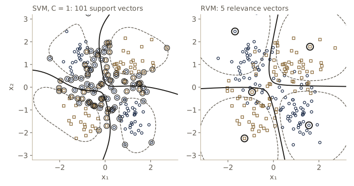
The RVM matches the SVM’s test error (slightly better, in fact) with five relevance vectors instead of about a hundred support vectors. Its probabilities come out of the model directly, and on the test set they are as good as those of the Platt-calibrated SVM, as measured by the cross-entropy. Notice where the relevance vectors are. The SVM’s support vectors crowd along the boundary. Four of the RVM’s five lie deep inside the four blobs, on their outer sides, where the predicted probabilities are within 0.003 of 0 or 1; only one sits near the boundary. The sparsity analysis explains the tendency. A kernel centered on a point near the boundary produces a vector \(\boldsymbol{\varphi}_i\) that straddles both classes and aligns poorly with the targets, so its quality factor tends to be low and it is pruned, while a kernel deep inside one class aligns well with that class’s labels.
For \(K > 2\) classes, the RVM uses the softmax model of module 04, \(y_k(\mathbf{x}) = \exp(a_k) / \sum_j \exp(a_j)\) with \(a_k = \mathbf{w}_k^{\mathrm{T}} \boldsymbol{\phi}(\mathbf{x})\), again with the Laplace approximation and IRLS. This treats all classes in one probabilistic model, which is more principled than combining two-class SVMs, but the Hessian now has size \(MK \times MK\), adding a factor of about \(K^3\) to the training cost.
In practice. The RVM’s main drawback is training time: the \(O(M^3)\) matrix work and a nonconvex objective, against the SVM’s convex QP. The trade usually still favors the RVM when prediction cost matters or when probabilities are needed, because it avoids cross-validation over \(C\) and \(\epsilon\) and produces far sparser models. The SVM remains the more common tool, helped by excellent convex solvers and a mature theory.
Summary
| Model | Objective | How it is fit | Sparsity comes from | Outputs |
|---|---|---|---|---|
| Hard-margin SVM | \(\min \tfrac12 \lVert \mathbf{w} \rVert^2\) s.t. \(t_n y_n \ge 1\) | dual QP (\(a_n \ge 0\)), e.g. SMO | complementary slackness: only points on the margin have \(a_n > 0\) | class (sign of \(y\)) |
| Soft-margin SVM | \(C \sum_n \xi_n + \tfrac12 \lVert \mathbf{w} \rVert^2\), i.e. hinge loss \(+ \lambda \lVert \mathbf{w} \rVert^2\) | dual QP with \(0 \le a_n \le C\) | the flat part of the hinge loss | class; probabilities only via Platt scaling |
| ν-SVM | \(\nu\) bounds the fractions of margin errors and support vectors | dual QP with an extra constraint | as above | class |
| SVR | \(C \sum_n E_\epsilon(y_n - t_n) + \tfrac12 \lVert \mathbf{w} \rVert^2\) | dual QP in \((a_n, \widehat{a}_n)\), same SMO | targets inside the ε-tube have \(a_n = \widehat{a}_n = 0\) | point prediction |
| RVM regression | evidence \(\ln \mathcal{N}(\mathbf{t} \mid \mathbf{0}, \beta^{-1}\mathbf{I} + \mathbf{\Phi} \mathbf{A}^{-1} \mathbf{\Phi}^{\mathrm{T}})\) | re-estimation \(\alpha_i = \gamma_i / m_i^2\), or the sequential algorithm | ARD: \(\alpha_i \to \infty\) when \(q_i^2 \le s_i\) | Gaussian predictive distribution |
| RVM classification | Laplace approximation to the evidence | IRLS inside, \(\alpha\) re-estimation outside | ARD, as above | class probabilities |
Ideas to carry forward:
- Duality and the KKT conditions turn a geometric requirement (maximize the margin) into a convex problem in kernel form, and complementary slackness explains the sparsity: inactive constraints get zero multipliers.
- Many classifiers are “loss plus regularizer”; the shape of the loss decides what the solution looks like. The hinge loss’s flat region gives sparsity, the logistic loss gives probabilities, and the squared loss is the wrong shape for classification.
- Sparsity can also come from Bayesian model selection. Giving each weight its own prior precision and maximizing the evidence switches off basis functions that do not earn their keep, measured by the quality and sparsity factors. The same idea (ARD) works for any linear combination of basis functions, and it returns in later modules.
- Localized basis functions give overconfident predictions far from the data. Gaussian processes avoid this at a higher cost, a trade-off between cost and calibrated uncertainty that recurs throughout the course.
Exercises
- For the hard-margin problem, suppose we fix the scale differently, requiring \(t_n y(\mathbf{x}_n) \ge \kappa\) for some \(\kappa > 0\) instead of 1. Show that the optimal decision boundary does not change, and describe how \(\mathbf{w}\), \(b\), and the multipliers \(a_n\) scale with \(\kappa\).
- Consider a training set with exactly one point of each class, \(\mathbf{x}_+\) and \(\mathbf{x}_-\), and a linear kernel. Solve the dual by hand (the equality constraint forces \(a_+ = a_-\)), and show that the maximum-margin boundary is the perpendicular bisector of the segment joining the two points, with margin half their distance. Check with
smo. - The SVM solution does not depend on the order of the training data; the perceptron’s does. Implement the perceptron of module 04 (with a bias) on
X_lin, run it on three random orderings of the data, and compare the three separating lines and their margins with the SVM’s margin of 0.7107. Which points determine each solution? - In the soft-margin SVM, prove that every point with \(t_n y(\mathbf{x}_n) < 1\) has \(a_n = C\), and every point with \(t_n y(\mathbf{x}_n) > 1\) has \(a_n = 0\). Then show that the fraction of training points with \(a_n = C\) is at most \(\sum_n a_n / (NC)\), and check the claim on the \(C\) sweep.
- The logistic loss \(\ln(1 + e^{-z})\) and the hinge loss \([1 - z]_+\) are both convex in \(z\). Show that a sum of convex losses of \(z_n = t_n y(\mathbf{x}_n)\) plus \(\lambda \lVert \mathbf{w} \rVert^2\) is a convex function of \((\mathbf{w}, b)\). Then compare the derivatives of the two losses with respect to \(z\), and explain what the comparison says about which training points influence each classifier.
- Kernelized logistic regression: write \(y(\mathbf{x}) = \sum_n c_n k(\mathbf{x}, \mathbf{x}_n) + b\), minimize \(\sum_n \ln(1 + e^{-t_n y_n}) + \lambda \mathbf{c}^{\mathrm{T}} \mathbf{K} \mathbf{c}\) with Newton’s method on
X_tr, and compare the number of coefficients \(c_n\) with magnitude above \(10^{-3}\) with the number of SVM support vectors. Which points get the largest \(\lvert c_n \rvert\)? - Derive the SVR dual from the Lagrangian given in the text, filling in the substitution step. Then prove that any point with \(\xi_n > 0\) has \(a_n = C\).
- Using
svr_fit, print how the number of support vectors, the number of targets outside the tube, and the rms error against \(\sin(2\pi x)\) vary as \(\epsilon\) goes from 0.05 to 0.5 at \(C = 1\). Relate what you see to the noise standard deviation of the data, 0.2. What happens when \(\epsilon\) exceeds the range of the residuals? - Using the finite-class PAC bound, how many examples suffice to learn, with \(\epsilon = 0.1\) and \(\delta = 0.05\), a conjunction of literals over 20 Boolean variables (each variable appears positively, negatively, or not at all)? How does the answer scale with the number of variables?
- Prove that \(\sum_i \gamma_i = \operatorname{Tr}(\beta \boldsymbol{\Sigma} \mathbf{\Phi}^{\mathrm{T}} \mathbf{\Phi})\) (hint: \(\beta \mathbf{\Phi}^{\mathrm{T}} \mathbf{\Phi} = \boldsymbol{\Sigma}^{-1} - \mathbf{A}\)), and that each \(\gamma_i\) lies in \([0, 1]\). Interpret \(\sum_i \gamma_i\) as an effective number of parameters, compute it for the fitted RVM, and compare it with the number of relevance vectors.
- Show that \(\lambda(\alpha_i) \to 0\) as \(\alpha_i \to \infty\), and explain why that is the right limit. Then, for the RVM fitted in the text, use
sparsity_qualityto plot \(\lambda\) against \(\ln \alpha_i\) for one relevance vector and for the pruned basis function with the largest \(q_i^2 / s_i\), and mark the closed-form optimum on the first curve. - Replace the Gaussian kernel basis in the RVM regression with a basis that is not a valid kernel, for example \(\phi_n(x) = \tanh(5(x - x_n))\) centered on each data point, and fit it with
rvm_regression. Does the RVM still work? Why could an SVM not use this “kernel”? - In your own words: explain to a classmate why the SVM’s support vectors sit near the decision boundary while the RVM’s relevance vectors sit away from it, even though both are “the training points that matter”.
Going further
- Bishop, Pattern Recognition and Machine Learning, chapter 7, the source for this module, and Appendix E on Lagrange multipliers. Exercises 7.1–7.5 cover the margin and the dual, 7.6–7.8 the loss view and regression, 7.9–7.17 the RVM evidence and the sparsity analysis, and 7.18–7.19 the classification RVM.
- Christopher J. C. Burges, “A tutorial on support vector machines for pattern recognition”, Data Mining and Knowledge Discovery, 1998 — a careful introduction that includes the VC-dimension bounds and the geometry of the margin.
- Corinna Cortes and Vladimir Vapnik, “Support-vector networks”, Machine Learning, 1995 — the soft-margin SVM with slack variables.
- Chih-Chung Chang and Chih-Jen Lin, “LIBSVM: a library for support vector machines”, ACM Transactions on Intelligent Systems and Technology, 2011 — the solver behind many SVM packages, with the details of SMO-type decomposition and working-set selection.
- Michael E. Tipping, “Sparse Bayesian learning and the relevance vector machine”, Journal of Machine Learning Research 1, 2001 — the original RVM paper; and Tipping and Faul, “Fast marginal likelihood maximisation for sparse Bayesian models”, AISTATS 2003, for the sequential algorithm.
- Bernhard Schölkopf and Alexander J. Smola, Learning with Kernels (MIT Press, 2002) — a book-length treatment of SVMs, ν-SVMs, one-class SVMs, and kernel design.
These notes follow the chapters of C. M. Bishop, Pattern Recognition and Machine Learning (Springer, 2006), the course text, which Microsoft Research makes freely available as a PDF. The explanations, code, figures, and exercises here are written for this course; the book remains the reference, with the full derivations and many more exercises.