CSE 474/574 · Module 06 · Week 6
Kernel Methods and Gaussian Processes
Dual representations, constructing valid kernels, radial basis functions and Nadaraya–Watson, and Gaussian processes for regression and classification.
Companion reading: Bishop, Pattern Recognition and Machine Learning, chapter 6, “Kernel Methods”
By the end of this module you can
- Derive the dual form of regularized least squares, implement kernel ridge regression, and check that it reproduces the primal ridge solution for an explicit feature map.
- Decide whether a function is a valid kernel by finding a feature map, by checking that its Gram matrices are positive semidefinite, or by building it from simpler kernels with the combination rules.
- Explain why the Gaussian kernel corresponds to an infinite-dimensional feature space, and describe kernels on non-vector objects and kernels derived from generative models.
- Implement radial basis function interpolation and the Nadaraya–Watson kernel regression model, and explain how the bandwidth trades bias against variance.
- Define a Gaussian process, sample functions from Gaussian process priors, and show that Bayesian linear regression is a Gaussian process with a particular kernel.
- Compute the predictive mean and variance of Gaussian process regression with a Cholesky factorization, and state its cost.
- Learn kernel hyperparameters by maximizing the log marginal likelihood with its gradient, and use automatic relevance determination to detect an irrelevant input.
- Build a Gaussian process classifier with the Laplace approximation, finding the posterior mode by Newton’s method and computing predictive probabilities.
Contents
- Kernels and memory-based methods
- Dual representations
- Constructing kernels
- Radial basis function networks
- Gaussian processes
- Linear regression revisited
- Sampling from a Gaussian process prior
- Gaussian process regression
- Bayesian linear regression as a special case
- The cost of exact inference
- Learning the hyperparameters
- Automatic relevance determination
- Gaussian processes for classification
- The Laplace approximation
- Connection to neural networks
- Summary
- Exercises
- Going further
The models of module 03 and module 04 are parametric: we choose basis functions \(\boldsymbol{\phi}(\mathbf{x})\), use the training data to fit a weight vector \(\mathbf{w}\) (or a posterior over it), and then throw the data away. Every prediction afterwards goes through \(\mathbf{w}\). The networks of module 05 work the same way, only with adaptive basis functions.
This module turns that picture around. We will see that many linear models can be rewritten so that the weights disappear and predictions are computed directly from the training points, through a function \(k(\mathbf{x}, \mathbf{x}')\) that measures how similar two inputs are. That function is a kernel, and once a model is written in terms of kernels we can swap in kernels whose feature spaces are enormous, even infinite, without ever computing a feature vector.
The first half of the module builds the tools: the dual representation of least squares, the rules that tell us which functions are valid kernels, and two classic kernel-based regressors (radial basis function networks and the Nadaraya–Watson model). The second half is about Gaussian processes, which put a prior directly on functions. They take the Bayesian linear regression of module 03 to its natural limit, give predictions with honest error bars, learn their own hyperparameters from the marginal likelihood, and extend to classification with the Laplace approximation of module 04. Module 07 then builds support vector machines on the same kernel ideas.
Kernels and memory-based methods
Some methods we have already met keep the training data around at prediction time. The kernel density estimator of module 02 places a bump on every training point, and the nearest-neighbor classifier compares a new input with every stored example. Such memory-based methods are quick to “train” (there is little to fit) but slow to predict, and they need a way to say how similar two inputs are.
The link between these methods and the parametric models is the kernel. For a fixed feature map \(\boldsymbol{\phi}(\mathbf{x})\), define
\[k(\mathbf{x}, \mathbf{x}') = \boldsymbol{\phi}(\mathbf{x})^{\mathrm{T}} \boldsymbol{\phi}(\mathbf{x}').\]It is symmetric, \(k(\mathbf{x}, \mathbf{x}') = k(\mathbf{x}', \mathbf{x})\). The simplest example uses the identity map \(\boldsymbol{\phi}(\mathbf{x}) = \mathbf{x}\) and gives the linear kernel \(k(\mathbf{x}, \mathbf{x}') = \mathbf{x}^{\mathrm{T}} \mathbf{x}'\).
The reason kernels are useful is the kernel trick (or kernel substitution): if an algorithm touches the inputs only through inner products \(\mathbf{x}^{\mathrm{T}} \mathbf{x}'\), we may replace every inner product by some other kernel \(k(\mathbf{x}, \mathbf{x}')\). The algorithm then runs, implicitly, in the feature space of that kernel. Kernel PCA in module 12 and the support vector machines of module 07 are built this way.
Two families of kernels come up constantly. A stationary kernel depends only on the difference of its arguments, \(k(\mathbf{x}, \mathbf{x}') = k(\mathbf{x} - \mathbf{x}')\), so it does not change if both inputs are shifted by the same amount. A radial (or homogeneous) kernel depends only on the distance, \(k(\mathbf{x}, \mathbf{x}') = k(\lVert \mathbf{x} - \mathbf{x}' \rVert)\). The Gaussian kernel below is both.
We start with imports and a few helpers used throughout the module. Most of the 1-D examples use the familiar noisy \(\sin(2\pi x)\) data of modules 01 and 03; each data set gets its own seeded generator so that the figure scripts can rebuild exactly the same points.
import numpy as np
import time
from scipy.linalg import solve_triangular
from scipy.optimize import minimize
from scipy.special import expit

np.set_printoptions(precision=4, suppress=True)
rng = np.random.default_rng(6)

def make_sin_data(N, rng, noise=0.2):
    """N inputs uniform on [0, 1], targets sin(2 pi x) + noise; X has shape (N, 1)."""
    x = rng.uniform(0, 1, N)
    t = np.sin(2 * np.pi * x) + noise * rng.standard_normal(N)
    return x[:, None], t

def sq_dists(X1, X2):
    """Squared Euclidean distances between the rows of X1 (N1, D) and X2 (N2, D)."""
    d = np.sum(X1**2, 1)[:, None] + np.sum(X2**2, 1)[None, :] - 2 * X1 @ X2.T
    return np.maximum(d, 0.0)          # clip tiny negative values caused by rounding

X_demo = np.array([[0.0], [0.5], [2.0]])
print(sq_dists(X_demo, X_demo))
[[0.   0.25 4.  ]
 [0.25 0.   2.25]
 [4.   2.25 0.  ]]
Dual representations
Regularized least squares in dual form
Take the regularized sum-of-squares error of module 03 for a linear model \(y(\mathbf{x}) = \mathbf{w}^{\mathrm{T}} \boldsymbol{\phi}(\mathbf{x})\) with \(M\) basis functions:
\[J(\mathbf{w}) = \frac{1}{2} \sum_{n=1}^{N} \left( \mathbf{w}^{\mathrm{T}} \boldsymbol{\phi}(\mathbf{x}_n) - t_n \right)^2 + \frac{\lambda}{2} \mathbf{w}^{\mathrm{T}} \mathbf{w}, \qquad \lambda > 0.\]Setting the gradient to zero gives \(\sum_n (\mathbf{w}^{\mathrm{T}} \boldsymbol{\phi}(\mathbf{x}_n) - t_n) \boldsymbol{\phi}(\mathbf{x}_n) + \lambda \mathbf{w} = \mathbf{0}\). We do not solve this for \(\mathbf{w}\) yet. Instead, read it as a statement about the shape of the solution:
\[\mathbf{w} = \sum_{n=1}^{N} a_n \boldsymbol{\phi}(\mathbf{x}_n) = \mathbf{\Phi}^{\mathrm{T}} \mathbf{a}, \qquad a_n = -\frac{1}{\lambda} \left( \mathbf{w}^{\mathrm{T}} \boldsymbol{\phi}(\mathbf{x}_n) - t_n \right),\]where \(\mathbf{\Phi}\) is the \(N \times M\) design matrix with rows \(\boldsymbol{\phi}(\mathbf{x}_n)^{\mathrm{T}}\). The optimal weight vector is a linear combination of the training feature vectors. The coefficients \(\mathbf{a} = (a_1, \dots, a_N)^{\mathrm{T}}\) are the dual variables, one per data point, in contrast to the \(M\) primal variables \(\mathbf{w}\).
To find \(\mathbf{a}\), write the definition of \(a_n\) for all \(n\) at once and substitute \(\mathbf{w} = \mathbf{\Phi}^{\mathrm{T}} \mathbf{a}\):
\[\lambda \mathbf{a} = \mathbf{t} - \mathbf{\Phi} \mathbf{w} = \mathbf{t} - \mathbf{\Phi} \mathbf{\Phi}^{\mathrm{T}} \mathbf{a} \quad\Longrightarrow\quad (\mathbf{K} + \lambda \mathbf{I}_N) \mathbf{a} = \mathbf{t},\]where \(\mathbf{K} = \mathbf{\Phi} \mathbf{\Phi}^{\mathrm{T}}\) is the \(N \times N\) Gram matrix, with entries \(K_{nm} = \boldsymbol{\phi}(\mathbf{x}_n)^{\mathrm{T}} \boldsymbol{\phi}(\mathbf{x}_m) = k(\mathbf{x}_n, \mathbf{x}_m)\). (Bishop §6.1 reaches the same equation by substituting \(\mathbf{w} = \mathbf{\Phi}^{\mathrm{T}} \mathbf{a}\) into \(J\) and minimizing over \(\mathbf{a}\).) The prediction at a new input is
\[y(\mathbf{x}) = \mathbf{w}^{\mathrm{T}} \boldsymbol{\phi}(\mathbf{x}) = \mathbf{a}^{\mathrm{T}} \mathbf{\Phi} \boldsymbol{\phi}(\mathbf{x}) = \mathbf{k}(\mathbf{x})^{\mathrm{T}} (\mathbf{K} + \lambda \mathbf{I}_N)^{-1} \mathbf{t},\]with \(\mathbf{k}(\mathbf{x})\) the vector of kernel values \(k_n(\mathbf{x}) = k(\mathbf{x}_n, \mathbf{x})\).
Result. Regularized least squares can be solved entirely with kernel evaluations: \(\mathbf{a} = (\mathbf{K} + \lambda \mathbf{I}_N)^{-1} \mathbf{t}\) and \(y(\mathbf{x}) = \sum_n a_n k(\mathbf{x}_n, \mathbf{x})\). The feature vectors never appear. This is kernel ridge regression.
Two remarks. First, the prediction is a linear combination of the training targets, \(y(\mathbf{x}) = \sum_n [\mathbf{k}(\mathbf{x})^{\mathrm{T}} (\mathbf{K} + \lambda \mathbf{I})^{-1}]_n \, t_n\): this is the equivalent-kernel view of module 03, written without basis functions. Second, the primal and dual answers agree because of the “push-through” identity \((\mathbf{\Phi}^{\mathrm{T}} \mathbf{\Phi} + \lambda \mathbf{I}_M)^{-1} \mathbf{\Phi}^{\mathrm{T}} = \mathbf{\Phi}^{\mathrm{T}} (\mathbf{\Phi} \mathbf{\Phi}^{\mathrm{T}} + \lambda \mathbf{I}_N)^{-1}\), which you can verify by multiplying both sides by the two bracketed matrices: \(\mathbf{\Phi}^{\mathrm{T}} (\mathbf{\Phi} \mathbf{\Phi}^{\mathrm{T}} + \lambda \mathbf{I}) = (\mathbf{\Phi}^{\mathrm{T}} \mathbf{\Phi} + \lambda \mathbf{I}) \mathbf{\Phi}^{\mathrm{T}}\).
Kernel ridge regression in code
Let us check the claim with an explicit feature map: polynomials \(\phi_j(x) = x^j\) for \(j = 0, \dots, 5\), fitted to 20 noisy points. We solve the \(M \times M\) primal system and the \(N \times N\) dual system and compare the weights and the predictions.
def poly_features(X, M):
    """Phi[n, j] = x_n ** j for j = 0..M-1 (1-D inputs, X of shape (N, 1))."""
    return X[:, [0]] ** np.arange(M)

def ridge_primal(Phi, t, lam):
    """w = (Phi^T Phi + lam I_M)^{-1} Phi^T t: an M x M system."""
    M = Phi.shape[1]
    return np.linalg.solve(Phi.T @ Phi + lam * np.eye(M), Phi.T @ t)

def ridge_dual(K, t, lam):
    """a = (K + lam I_N)^{-1} t: an N x N system."""
    return np.linalg.solve(K + lam * np.eye(len(t)), t)

X_tr, t_tr = make_sin_data(20, np.random.default_rng(1))
M, lam = 6, 1e-3
Phi = poly_features(X_tr, M)
X_new = np.linspace(0, 1, 7)[:, None]

w = ridge_primal(Phi, t_tr, lam)
a = ridge_dual(Phi @ Phi.T, t_tr, lam)                 # Gram matrix K = Phi Phi^T
k_new = poly_features(X_new, M) @ Phi.T                # k_new[i, n] = k(x_new_i, x_n)

print("max |w - Phi^T a|          :", f"{np.max(np.abs(w - Phi.T @ a)):.2e}")
print("predictions (primal)       :", poly_features(X_new, M) @ w)
print("predictions (dual)         :", k_new @ a)
max |w - Phi^T a|          : 8.14e-12
predictions (primal)       : [ 0.4357  0.8077  0.6247  0.0507 -0.5882 -0.764   0.2931]
predictions (dual)         : [ 0.4357  0.8077  0.6247  0.0507 -0.5882 -0.764   0.2931]
The two routes give the same weights and the same predictions, up to rounding. Notice what the dual route needed: only the \(20 \times 20\) matrix of inner products and the inner products between new and old inputs.
That matters as soon as we pick a kernel whose features we cannot list. The Gaussian kernel \(k(\mathbf{x}, \mathbf{x}') = \exp(-\lVert \mathbf{x} - \mathbf{x}' \rVert^2 / 2\ell^2)\), studied in the next section, has an infinite-dimensional feature space, so the primal route is closed; the dual route is not.
def k_gauss(X1, X2, ell=1.0):
    """Gaussian kernel exp(-||x - x'||^2 / (2 ell^2)) between rows of X1 and X2."""
    return np.exp(-sq_dists(X1, X2) / (2 * ell**2))

X_grid = np.linspace(0, 1, 201)[:, None]
y_true = np.sin(2 * np.pi * X_grid[:, 0])
for ell in [0.02, 0.1, 0.5]:
    a = ridge_dual(k_gauss(X_tr, X_tr, ell), t_tr, lam=0.04)
    y = k_gauss(X_grid, X_tr, ell) @ a
    rmse = np.sqrt(np.mean((y - y_true) ** 2))
    print(f"ell = {ell:4.2f}   RMSE against sin(2 pi x) on a grid: {rmse:.3f}")
ell = 0.02   RMSE against sin(2 pi x) on a grid: 0.439
ell = 0.10   RMSE against sin(2 pi x) on a grid: 0.199
ell = 0.50   RMSE against sin(2 pi x) on a grid: 0.269
The length-scale \(\ell\) says how far the influence of one training point reaches. With \(\ell = 0.02\) each point affects only a tiny neighborhood, and between points the prediction sags back toward zero; with \(\ell = 0.5\) the fit is too stiff to follow a full period of the sine. The middle value does well. Choosing \(\ell\) and \(\lambda\) is a model-selection problem, and the Gaussian-process view later in the module gives a principled way to do it.
Primal or dual: the cost
The primal solution costs \(O(NM^2)\) to form \(\mathbf{\Phi}^{\mathrm{T}} \mathbf{\Phi}\) and \(O(M^3)\) to solve; the dual costs \(O(N^2 M)\) to form \(\mathbf{K}\) (or \(O(N^2)\) kernel evaluations) and \(O(N^3)\) to solve. With many data points and few features the primal wins; with few data points and many features, or with a kernel whose feature space is infinite, the dual is the only practical choice. A quick timing makes the point (your times will differ; the ratio is what matters).
def time_ridge(N, M, rng):
    Phi = rng.standard_normal((N, M))
    t = rng.standard_normal(N)
    t0 = time.perf_counter()
    w = ridge_primal(Phi, t, 1.0)
    t1 = time.perf_counter()
    a = ridge_dual(Phi @ Phi.T, t, 1.0)
    t2 = time.perf_counter()
    print(f"N = {N:5d}, M = {M:5d}:  primal {(t1 - t0) * 1e3:7.1f} ms   "
          f"dual {(t2 - t1) * 1e3:7.1f} ms   same w: {np.allclose(w, Phi.T @ a)}")

time_ridge(2000, 20, rng)
time_ridge(20, 2000, rng)
N =  2000, M =    20:  primal     0.2 ms   dual   145.4 ms   same w: True
N =    20, M =  2000:  primal   104.5 ms   dual     0.2 ms   same w: True
The dual system is \(2000 \times 2000\) in the first case and \(20 \times 20\) in the second, and the timings flip accordingly; both routes give the same weights.
Note. The dual form is not a trick special to least squares. Any model whose optimal weights are a combination of the training feature vectors can be written this way. Bishop’s exercise 6.2 does it for the perceptron of module 04, and the representer theorem (Bishop exercise 6.16) shows that it holds whenever the error depends on \(\mathbf{w}\) only through the values \(\mathbf{w}^{\mathrm{T}} \boldsymbol{\phi}(\mathbf{x}_n)\) plus an increasing function of \(\lVert \mathbf{w} \rVert\). Support vector machines (module 07) are the most famous example.
Constructing kernels
To use kernel substitution we need valid kernels: functions that really are an inner product in some feature space. There are three ways to get one.
Kernels from feature maps
The first way is to choose the features and compute the inner product. With \(M\) basis functions on a 1-D input, \(k(x, x') = \sum_{i=1}^{M} \phi_i(x) \phi_i(x')\); polynomial, Gaussian, and sigmoidal basis functions each give a different kernel shape.
It also works the other way: sometimes a kernel written in closed form turns out to have a simple feature map. Take \(k(\mathbf{x}, \mathbf{z}) = (\mathbf{x}^{\mathrm{T}} \mathbf{z})^2\) in two dimensions. Expanding the square,
\[\begin{aligned} (x_1 z_1 + x_2 z_2)^2 &= x_1^2 z_1^2 + 2 x_1 x_2 z_1 z_2 + x_2^2 z_2^2 = \boldsymbol{\phi}(\mathbf{x})^{\mathrm{T}} \boldsymbol{\phi}(\mathbf{z}), \\ \boldsymbol{\phi}(\mathbf{x}) &= \left( x_1^2, \sqrt{2}\, x_1 x_2, x_2^2 \right)^{\mathrm{T}}. \end{aligned}\]So this kernel computes, with one inner product and one squaring, the inner product of all second-order monomials (with a particular weighting).
def phi_quad(X):
    """Explicit features of the kernel (x^T z)^2 for 2-D inputs."""
    return np.column_stack([X[:, 0]**2, np.sqrt(2) * X[:, 0] * X[:, 1], X[:, 1]**2])

X2 = rng.standard_normal((5, 2))
K_closed = (X2 @ X2.T) ** 2
K_features = phi_quad(X2) @ phi_quad(X2).T
diff = np.max(np.abs(K_closed - K_features))
print(f"max difference between (x^T z)^2 and phi(x)^T phi(z): {diff:.2e}")
max difference between (x^T z)^2 and phi(x)^T phi(z): 8.88e-16
More generally, \((\mathbf{x}^{\mathrm{T}} \mathbf{x}')^M\) contains all monomials of degree exactly \(M\), and \((\mathbf{x}^{\mathrm{T}} \mathbf{x}' + c)^M\) with \(c > 0\) contains all monomials up to degree \(M\). In \(D\) dimensions the number of such monomials grows like \(D^M\), while evaluating the kernel still costs \(O(D)\).
The test: positive semidefinite Gram matrices
The second way is to write down a function and check that it is a kernel without finding its features. Here is the criterion.
Definition. A symmetric function \(k(\mathbf{x}, \mathbf{x}')\) is a valid kernel (a positive semidefinite kernel) if, for every finite set of inputs \(\mathbf{x}_1, \dots, \mathbf{x}_N\), the Gram matrix \(K_{nm} = k(\mathbf{x}_n, \mathbf{x}_m)\) is positive semidefinite: \(\mathbf{c}^{\mathrm{T}} \mathbf{K} \mathbf{c} \ge 0\) for every \(\mathbf{c} \in \mathbb{R}^N\), or equivalently all eigenvalues of \(\mathbf{K}\) are nonnegative.
Necessity is one line. If \(k(\mathbf{x}, \mathbf{x}') = \boldsymbol{\phi}(\mathbf{x})^{\mathrm{T}} \boldsymbol{\phi}(\mathbf{x}')\), then
\[\mathbf{c}^{\mathrm{T}} \mathbf{K} \mathbf{c} = \sum_{n,m} c_n c_m \boldsymbol{\phi}(\mathbf{x}_n)^{\mathrm{T}} \boldsymbol{\phi}(\mathbf{x}_m) = \Big\lVert \sum_n c_n \boldsymbol{\phi}(\mathbf{x}_n) \Big\rVert^2 \ge 0.\]The converse, that every such function is an inner product in some (possibly infinite-dimensional) feature space, is a standard theorem of functional analysis (Mercer’s theorem and its relatives); Shawe-Taylor and Cristianini (2004) treat it in detail. We will use it without proof.
A numerical check cannot prove validity, since it looks at one set of points, but it can refute it: a single Gram matrix with a negative eigenvalue shows that a function is not a kernel. Two tempting candidates fail. The Euclidean distance \(\lVert \mathbf{x} - \mathbf{x}' \rVert\) has zeros on the diagonal, so its Gram matrix has trace zero, and a nonzero symmetric matrix with trace zero must have a negative eigenvalue. The sigmoidal kernel \(\tanh(a \mathbf{x}^{\mathrm{T}} \mathbf{x}' + b)\) looks like a neural-network unit and has been used in practice, but its Gram matrices are in general not positive semidefinite.
X30 = np.random.default_rng(3).uniform(-1, 1, (30, 2))
candidates = {
    "linear  x^T x'":              X30 @ X30.T,
    "poly    (x^T x' + 1)^3":      (X30 @ X30.T + 1) ** 3,
    "Gaussian, ell = 0.5":         k_gauss(X30, X30, 0.5),
    "distance ||x - x'||":         np.sqrt(sq_dists(X30, X30)),
    "sigmoid tanh(x^T x' - 1)":    np.tanh(X30 @ X30.T - 1),
}
for name, K in candidates.items():
    eig = np.linalg.eigvalsh(K)
    print(f"{name:27s} smallest eigenvalue {eig[0]:10.2e}   largest {eig[-1]:8.2f}")
linear  x^T x'              smallest eigenvalue  -1.27e-15   largest    10.46
poly    (x^T x' + 1)^3      smallest eigenvalue  -7.23e-15   largest    49.54
Gaussian, ell = 0.5         smallest eigenvalue   3.30e-08   largest     9.47
distance ||x - x'||         smallest eigenvalue  -1.01e+01   largest    29.46
sigmoid tanh(x^T x' - 1)    smallest eigenvalue  -2.13e+01   largest     4.74
The first three pass. The linear and cubic kernels have feature spaces of dimension 2 and 10, so their \(30 \times 30\) Gram matrices have rank at most 2 and 10 and most of their eigenvalues are exactly zero; rounding turns a few of those into numbers like \(-10^{-15}\), which is floating-point noise. The Gaussian’s smallest eigenvalue is tiny but positive. The distance and the sigmoid have clearly negative eigenvalues, about −10 and −21. What goes wrong if we use them anyway? The eigenvector \(\mathbf{c}\) of a negative eigenvalue gives \(\mathbf{c}^{\mathrm{T}} \mathbf{K} \mathbf{c} < 0\), a “squared length” that is negative, so there is no feature space in which the function is an inner product. In a Gaussian process, where \(\mathbf{K}\) is a covariance matrix, it would be a variance below zero.
K_bad = candidates["sigmoid tanh(x^T x' - 1)"]
eig, vecs = np.linalg.eigh(K_bad)
c = vecs[:, 0]                          # eigenvector of the most negative eigenvalue
print(f"c^T K c = {c @ K_bad @ c:.3f}")
try:
    np.linalg.cholesky(K_bad + 1e-6 * np.eye(30))
except np.linalg.LinAlgError as err:
    print("Cholesky factorization fails:", err)
c^T K c = -21.315
Cholesky factorization fails: Matrix is not positive definite
Watch out. Positive semidefinite is a statement about eigenvalues, not about entries. The matrix with rows (1, 2) and (2, 1) has only positive entries and an eigenvalue of −1; the matrix with rows (1, −0.5) and (−0.5, 1) has a negative entry and is positive definite. A kernel may take negative values (the linear kernel does) and still be valid.
Building new kernels from old
The third way, and the most useful in practice, is to assemble kernels from pieces that are known to be valid. If \(k_1\) and \(k_2\) are valid kernels, so are the following (Bishop lists them as equations 6.13–6.22):
| New kernel | Condition | Why it is valid |
|---|---|---|
| \(c\, k_1(\mathbf{x}, \mathbf{x}')\) | \(c > 0\) | scale the features by \(\sqrt{c}\) |
| \(f(\mathbf{x})\, k_1(\mathbf{x}, \mathbf{x}')\, f(\mathbf{x}')\) | any function \(f\) | features \(f(\mathbf{x}) \boldsymbol{\phi}_1(\mathbf{x})\) |
| \(k_1 + k_2\) | stack the two feature vectors | |
| \(k_1 \, k_2\) | features are all products \(\phi_{1i}(\mathbf{x}) \phi_{2j}(\mathbf{x})\) | |
| \(q(k_1)\) | \(q\) a polynomial with nonnegative coefficients | sums, products, and positive constants |
| \(\exp(k_1)\) | limit of the polynomials \(\sum_{j \le J} k_1^j / j!\) | |
| \(k_3(\boldsymbol{\psi}(\mathbf{x}), \boldsymbol{\psi}(\mathbf{x}'))\) | \(k_3\) valid on the range of \(\boldsymbol{\psi}\) | a Gram matrix of \(k_3\) on the points \(\boldsymbol{\psi}(\mathbf{x}_n)\) |
| \(\mathbf{x}^{\mathrm{T}} \mathbf{A} \mathbf{x}'\) | \(\mathbf{A}\) symmetric positive semidefinite | features \(\mathbf{\Lambda}^{1/2} \mathbf{U}^{\mathrm{T}} \mathbf{x}\) with \(\mathbf{A} = \mathbf{U} \mathbf{\Lambda} \mathbf{U}^{\mathrm{T}}\) |
| \(k_a(\mathbf{x}_a, \mathbf{x}_a') + k_b(\mathbf{x}_b, \mathbf{x}_b')\) | \(\mathbf{x} = (\mathbf{x}_a, \mathbf{x}_b)\) | sum rule applied to kernels on parts of \(\mathbf{x}\) |
| \(k_a(\mathbf{x}_a, \mathbf{x}_a')\, k_b(\mathbf{x}_b, \mathbf{x}_b')\) | \(\mathbf{x} = (\mathbf{x}_a, \mathbf{x}_b)\) | product rule applied to parts |
The product rule deserves one more sentence, because it is the least obvious. If \(k_1 = \boldsymbol{\phi}^{\mathrm{T}} \boldsymbol{\phi}'\) and \(k_2 = \boldsymbol{\psi}^{\mathrm{T}} \boldsymbol{\psi}'\), then \(k_1 k_2 = \sum_i \sum_j \phi_i(\mathbf{x}) \psi_j(\mathbf{x}) \, \phi_i(\mathbf{x}') \psi_j(\mathbf{x}')\), an inner product of the \(M_1 M_2\) products. (For matrices this is the Schur product theorem: the elementwise product of two positive semidefinite matrices is positive semidefinite.) With these rules we can design kernels for a task, combining, say, a smooth trend with a periodic component, and know they are valid without checking anything.
K_lin = X30 @ X30.T
K_g = k_gauss(X30, X30, 0.5)
built = {
    "3 * Gaussian + linear": 3 * K_g + K_lin,
    "Gaussian * (linear + 1)^2": K_g * (K_lin + 1) ** 2,
    "exp(linear)": np.exp(K_lin),
}
for name, K in built.items():
    print(f"{name:26s} smallest eigenvalue {np.linalg.eigvalsh(K)[0]:10.2e}")
3 * Gaussian + linear      smallest eigenvalue   1.00e-07
Gaussian * (linear + 1)^2  smallest eigenvalue   2.40e-07
exp(linear)                smallest eigenvalue   6.56e-12
The Gaussian kernel
The kernel we will use most is the Gaussian kernel (also called the squared-exponential or RBF kernel)
\[k(\mathbf{x}, \mathbf{x}') = \exp\left( -\frac{\lVert \mathbf{x} - \mathbf{x}' \rVert^2}{2 \ell^2} \right),\]with length-scale \(\ell > 0\) (Bishop writes \(\sigma\)). It is not a probability density here, so there is no normalizing constant. To see that it is valid, expand the square, \(\lVert \mathbf{x} - \mathbf{x}' \rVert^2 = \mathbf{x}^{\mathrm{T}} \mathbf{x} - 2 \mathbf{x}^{\mathrm{T}} \mathbf{x}' + \mathbf{x}'^{\mathrm{T}} \mathbf{x}'\), which splits the kernel into three factors:
\[k(\mathbf{x}, \mathbf{x}') = \underbrace{\exp\left( -\frac{\mathbf{x}^{\mathrm{T}} \mathbf{x}}{2\ell^2} \right)}_{f(\mathbf{x})} \; \exp\left( \frac{\mathbf{x}^{\mathrm{T}} \mathbf{x}'}{\ell^2} \right) \; \underbrace{\exp\left( -\frac{\mathbf{x}'^{\mathrm{T}} \mathbf{x}'}{2\ell^2} \right)}_{f(\mathbf{x}')}.\]The middle factor is the exponential of a scaled linear kernel, valid by the exp rule, and the outer factors fit the \(f(\mathbf{x}) k_1 f(\mathbf{x}')\) rule. So the Gaussian kernel is valid.
The same expansion exposes its feature space. In one dimension, expand the middle factor as a power series, \(\exp(x x' / \ell^2) = \sum_{j=0}^{\infty} (x x')^j / (\ell^{2j} j!)\). Then
\[k(x, x') = \sum_{j=0}^{\infty} \phi_j(x) \phi_j(x'), \qquad \phi_j(x) = e^{-x^2 / 2\ell^2} \frac{x^j}{\ell^j \sqrt{j!}}, \quad j = 0, 1, 2, \dots\]There is one feature for every power of \(x\): the feature space is infinite-dimensional. Truncating the sum gives a finite approximation, which converges quickly for inputs of moderate size.
from math import factorial

def phi_gauss_truncated(x, J, ell=1.0):
    """First J features of the 1-D Gaussian kernel, exp(-x^2/2l^2) (x/l)^j / sqrt(j!)."""
    j = np.arange(J)
    norms = np.sqrt([float(factorial(i)) for i in j])
    return np.exp(-x[:, None]**2 / (2 * ell**2)) * (x[:, None] / ell) ** j / norms

x = np.linspace(-2, 2, 41)
K_exact = k_gauss(x[:, None], x[:, None], 1.0)
for J in [2, 5, 10, 20, 30]:
    F = phi_gauss_truncated(x, J)
    print(f"J = {J:2d} features: max error {np.max(np.abs(F @ F.T - K_exact)):.1e}")
J =  2 features: max error 9.1e-01
J =  5 features: max error 3.7e-01
J = 10 features: max error 8.1e-03
J = 20 features: max error 1.0e-08
J = 30 features: max error 5.6e-16
Inputs far from the origin need more terms (the neglected terms involve \((x x' / \ell^2)^j / j!\)), but for any fixed inputs the error goes to zero.
The Gaussian kernel is not tied to Euclidean distance. Because \(\lVert \mathbf{x} - \mathbf{x}' \rVert^2\) is itself written with inner products, we can substitute any valid kernel \(\kappa\) for them:
\[k(\mathbf{x}, \mathbf{x}') = \exp\left( -\frac{1}{2\ell^2} \left[ \kappa(\mathbf{x}, \mathbf{x}) - 2\kappa(\mathbf{x}, \mathbf{x}') + \kappa(\mathbf{x}', \mathbf{x}') \right] \right),\]which is a Gaussian kernel on the squared distance in the feature space of \(\kappa\).
Kernels on sets, strings, and other objects
Nothing in the definition of a kernel requires \(\mathbf{x}\) to be a vector of numbers. Kernels have been defined on strings, trees, graphs, sets, and whole documents, and a kernel method then works on those objects directly. That extension is one of the main practical payoffs of the kernel view.
A small example: fix a finite set \(D\) and let the inputs be its subsets. The function
\[k(A_1, A_2) = 2^{\lvert A_1 \cap A_2 \rvert},\]where \(\lvert A \rvert\) is the number of elements of \(A\), is a valid kernel. The feature map has one coordinate for every subset \(U\) of \(D\), with \(\phi_U(A) = 1\) if \(U \subseteq A\) and 0 otherwise. Then \(\boldsymbol{\phi}(A_1)^{\mathrm{T}} \boldsymbol{\phi}(A_2)\) counts the subsets \(U\) contained in both \(A_1\) and \(A_2\), that is, the subsets of \(A_1 \cap A_2\), and there are \(2^{\lvert A_1 \cap A_2 \rvert}\) of them. We can check this by brute force on a five-element set, storing each subset as a bit mask.
n_elems = 5
subsets = range(2 ** n_elems)       # bit mask b stands for the set {i : bit i of b is 1}

def set_kernel(A1, A2):
    return 2 ** bin(A1 & A2).count("1")         # 2^{|A1 intersect A2|}

def set_features(A):
    """phi_U(A) = 1 if U is a subset of A, for all 32 subsets U."""
    return np.array([1.0 if (U & A) == U else 0.0 for U in subsets])

K_set = np.array([[set_kernel(A1, A2) for A2 in subsets] for A1 in subsets])
F = np.array([set_features(A) for A in subsets])
print("kernel equals phi^T phi on all 32 x 32 pairs:", np.array_equal(K_set, F @ F.T))
print(f"smallest eigenvalue of the Gram matrix: {np.linalg.eigvalsh(K_set)[0]:.3f}")
kernel equals phi^T phi on all 32 x 32 pairs: True
smallest eigenvalue of the Gram matrix: 0.008
Kernels from generative models
Generative models (module 04) handle missing data and variable-length sequences naturally; discriminative models tend to classify better. One way to get some of both is to build a kernel from a generative model and use it in a discriminative method.
The simplest choice is \(k(\mathbf{x}, \mathbf{x}') = p(\mathbf{x}) p(\mathbf{x}')\), an inner product in a one-dimensional feature space: two inputs are similar if both are probable. A richer choice sums over the components of a mixture, \(k(\mathbf{x}, \mathbf{x}') = \sum_i p(\mathbf{x} \mid i)\, p(\mathbf{x}' \mid i)\, p(i)\), which is valid by the sum and scaling rules; two inputs are similar if they are likely under the same components. Replacing the sum by an integral over a continuous latent variable, or by a sum over hidden state sequences of a hidden Markov model (module 13), gives kernels between vectors or between whole sequences.
A different construction is the Fisher kernel. For a parametric model \(p(\mathbf{x} \mid \boldsymbol{\theta})\), the Fisher score \(\mathbf{g}(\boldsymbol{\theta}, \mathbf{x}) = \nabla_{\boldsymbol{\theta}} \ln p(\mathbf{x} \mid \boldsymbol{\theta})\) says how the log-likelihood of \(\mathbf{x}\) would change if we nudged each parameter; it maps any input, even a sequence, to a vector with one entry per parameter. The Fisher kernel is
\[k(\mathbf{x}, \mathbf{x}') = \mathbf{g}(\boldsymbol{\theta}, \mathbf{x})^{\mathrm{T}} \mathbf{F}^{-1} \mathbf{g}(\boldsymbol{\theta}, \mathbf{x}'), \qquad \mathbf{F} = \mathbb{E}_{\mathbf{x}} \left[ \mathbf{g}(\boldsymbol{\theta}, \mathbf{x}) \mathbf{g}(\boldsymbol{\theta}, \mathbf{x})^{\mathrm{T}} \right],\]where \(\mathbf{F}\) is the Fisher information matrix. Weighting by \(\mathbf{F}^{-1}\) makes the kernel unchanged if the model is reparameterized by any smooth invertible map \(\boldsymbol{\theta} \to \boldsymbol{\psi}(\boldsymbol{\theta})\). In practice \(\mathbf{F}\) is replaced by the sample average of \(\mathbf{g} \mathbf{g}^{\mathrm{T}}\) over the training data (which whitens the scores) or dropped altogether. As a tiny example, for a 1-D Gaussian with unknown mean \(\mu\) and known variance \(s^2\), the score is \((x - \mu)/s^2\), the Fisher information is \(1/s^2\), and the Fisher kernel is \((x - \mu)(x' - \mu)/s^2\): a linear kernel on inputs centered at the model’s mean.
Radial basis function networks
In module 03 we used Gaussian basis functions without asking where the idea came from. A radial basis function depends only on the distance from a center, \(\phi_j(\mathbf{x}) = h(\lVert \mathbf{x} - \boldsymbol{\mu}_j \rVert)\). Radial basis functions arise in several ways, and each connects to kernels.
Exact interpolation
The original use was interpolation: given inputs \(\mathbf{x}_1, \dots, \mathbf{x}_N\) and targets \(t_1, \dots, t_N\), find a smooth \(f\) with \(f(\mathbf{x}_n) = t_n\) exactly. Put one basis function on every data point,
\[f(\mathbf{x}) = \sum_{n=1}^{N} w_n \, h(\lVert \mathbf{x} - \mathbf{x}_n \rVert),\]and solve the \(N\) equations \(\mathbf{H} \mathbf{w} = \mathbf{t}\) for the \(N\) weights, where \(H_{nm} = h(\lVert \mathbf{x}_n - \mathbf{x}_m \rVert)\). With a Gaussian \(h\), \(\mathbf{H}\) is exactly the Gram matrix of the Gaussian kernel, and interpolation is kernel ridge regression with \(\lambda = 0\). For noisy targets that is an overfit, as the next cell shows.
X_rbf, t_rbf = make_sin_data(12, np.random.default_rng(4))
H = k_gauss(X_rbf, X_rbf, ell=0.1)
w_interp = np.linalg.solve(H, t_rbf)                # exact interpolation
a_ridge = ridge_dual(H, t_rbf, lam=0.04)            # regularized: lambda = noise variance

for name, coef in [("interpolation", w_interp), ("ridge, lambda = 0.04", a_ridge)]:
    y_train = H @ coef
    y_grid = k_gauss(X_grid, X_rbf, 0.1) @ coef
    resid = np.max(np.abs(y_train - t_rbf))
    rmse = np.sqrt(np.mean((y_grid - y_true) ** 2))
    print(f"{name:21s} max train residual {resid:.1e}   grid RMSE vs sin {rmse:.3f}   "
          f"max |w| {np.max(np.abs(coef)):6.1f}")
print(f"condition number of H: {np.linalg.cond(H):.1e}")
interpolation         max train residual 4.3e-14   grid RMSE vs sin 0.646   max |w|  239.6
ridge, lambda = 0.04  max train residual 1.2e-01   grid RMSE vs sin 0.241   max |w|    3.0
condition number of H: 3.1e+04
The interpolant passes through every noisy target (residuals of order \(10^{-14}\)), needs weights in the hundreds to do it, and ends up much further from the true curve than the regularized fit: a grid RMSE of 0.65 against 0.24. Regularization theory gives a second motivation for the same expansion: minimizing a sum of squares plus a smoothness penalty written with a differential operator yields a solution that is a sum of the operator’s Green’s functions, one centered on each data point, and for a rotation-invariant operator these are radial (Bishop §6.3 has the references).
Normalized basis functions and fewer centers
A third motivation comes from noise on the inputs. If each input is observed with noise \(\boldsymbol{\xi}\) of density \(\nu(\boldsymbol{\xi})\) and we minimize the expected squared error, the calculus of variations (Bishop §6.3, exercise 6.17) gives
\[y(\mathbf{x}) = \sum_{n=1}^{N} t_n \, h(\mathbf{x} - \mathbf{x}_n), \qquad h(\mathbf{x} - \mathbf{x}_n) = \frac{\nu(\mathbf{x} - \mathbf{x}_n)}{\sum_{m} \nu(\mathbf{x} - \mathbf{x}_m)}.\]These basis functions are normalized: they sum to one at every \(\mathbf{x}\). Normalization avoids regions of input space where every basis function is nearly zero, where an unnormalized model would predict about zero (or whatever the bias says) regardless of the data. The same model reappears in the next subsection from a density-estimation argument.
A model with one basis function per data point is slow to evaluate when \(N\) is large. The classic RBF network therefore uses \(M < N\) centers: choose the centers from the inputs alone (a random subset of the data, a greedy method called orthogonal least squares that adds the point that most reduces the error, or the cluster centers from K-means of module 09), keep them fixed, and fit the output weights by linear least squares exactly as in module 03.
The Nadaraya–Watson model
Now the density-estimation route. Model the joint density of input and target with a kernel density estimator (module 02), one component per training pair:
\[p(\mathbf{x}, t) = \frac{1}{N} \sum_{n=1}^{N} f(\mathbf{x} - \mathbf{x}_n, t - t_n),\]where \(f\) is a density that we assume has zero mean in \(t\), \(\int f(\mathbf{x}, t)\, t \, dt = 0\). The regression function is the conditional mean,
\[y(\mathbf{x}) = \mathbb{E}[t \mid \mathbf{x}] = \frac{\int t \, p(\mathbf{x}, t)\, dt}{\int p(\mathbf{x}, t)\, dt}.\]In the \(n\)th term of the numerator substitute \(u = t - t_n\): \(\int t f(\mathbf{x} - \mathbf{x}_n, t - t_n)\, dt = \int (u + t_n) f(\mathbf{x} - \mathbf{x}_n, u)\, du = t_n \, g(\mathbf{x} - \mathbf{x}_n)\), where \(g(\mathbf{x}) = \int f(\mathbf{x}, u)\, du\) is the marginal of \(f\) over the target and the zero-mean assumption removed the \(u\) term. The denominator is \(\sum_m g(\mathbf{x} - \mathbf{x}_m)\). So
\[y(\mathbf{x}) = \sum_{n=1}^{N} k(\mathbf{x}, \mathbf{x}_n)\, t_n, \qquad k(\mathbf{x}, \mathbf{x}_n) = \frac{g(\mathbf{x} - \mathbf{x}_n)}{\sum_{m=1}^{N} g(\mathbf{x} - \mathbf{x}_m)}.\]This is the Nadaraya–Watson model, or kernel regression. The prediction is a weighted average of the training targets, with weights that are larger for nearby inputs and sum to one, \(\sum_n k(\mathbf{x}, \mathbf{x}_n) = 1\). (Here “kernel” means a normalized weighting function; it is not required to be positive semidefinite.)
The model gives more than a mean. The same construction yields the whole conditional density \(p(t \mid \mathbf{x}) = p(\mathbf{x}, t) / \int p(\mathbf{x}, t)\, dt\). If \(f\) is an isotropic Gaussian with variance \(h^2\) in every direction of \((\mathbf{x}, t)\), then \(g\) is a Gaussian of width \(h\) and
\[p(t \mid \mathbf{x}) = \sum_{n=1}^{N} k(\mathbf{x}, \mathbf{x}_n) \, \mathcal{N}(t \mid t_n, h^2),\]a mixture of Gaussians centered on the training targets. Its mean is \(y(\mathbf{x})\) and its variance is \(h^2 + \sum_n k(\mathbf{x}, \mathbf{x}_n) t_n^2 - y(\mathbf{x})^2\) (the variance of a mixture is the average within-component variance plus the spread of the component means). We compute the weights in log space, since far from the data every \(g\) underflows.
def nadaraya_watson(X, t, X_new, h):
    """Kernel regression with a Gaussian of width h in (x, t).
    Returns the conditional mean and variance of p(t | x) at each row of X_new."""
    log_g = -sq_dists(X_new, X) / (2 * h**2)     # log g(x - x_n), up to a constant
    log_g -= log_g.max(axis=1, keepdims=True)    # stabilize before exponentiating
    weights = np.exp(log_g)
    weights /= weights.sum(axis=1, keepdims=True)   # k(x, x_n); each row sums to 1
    mean = weights @ t
    var = h**2 + weights @ t**2 - mean**2        # variance of the Gaussian mixture
    return mean, var

X_nw, t_nw = make_sin_data(30, np.random.default_rng(5))
for h in [0.02, 0.07, 0.25]:
    mean, var = nadaraya_watson(X_nw, t_nw, X_grid, h)
    mean_tr, _ = nadaraya_watson(X_nw, t_nw, X_nw, h)
    train_rmse = np.sqrt(np.mean((mean_tr - t_nw) ** 2))
    grid_rmse = np.sqrt(np.mean((mean - y_true) ** 2))
    print(f"h = {h:4.2f}   train RMSE {train_rmse:.3f}   "
          f"grid RMSE vs sin {grid_rmse:.3f}   mean predictive sd {np.mean(np.sqrt(var)):.3f}")
h = 0.02   train RMSE 0.132   grid RMSE vs sin 0.203   mean predictive sd 0.138
h = 0.07   train RMSE 0.200   grid RMSE vs sin 0.159   mean predictive sd 0.320
h = 0.25   train RMSE 0.408   grid RMSE vs sin 0.419   mean predictive sd 0.600
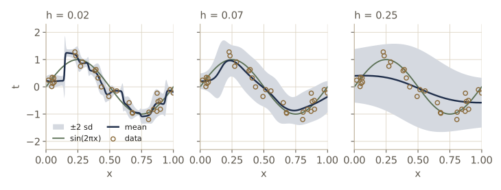
The bandwidth \(h\) plays the role that \(\lambda\) and \(\ell\) played for kernel ridge regression: a small \(h\) gives low bias and high variance (the training error is small, the curve is jagged), a large \(h\) the reverse. The conditional variance also reflects \(h\): every mixture component has variance \(h^2\), and a wide kernel averages targets from different parts of the sine, which adds spread.
Nadaraya–Watson needs no training at all, but every prediction touches all \(N\) training points. A natural extension fits a Gaussian mixture with fewer, more flexible components to \(p(\mathbf{x}, t)\) (module 09) and conditions it on \(\mathbf{x}\): training becomes more expensive, prediction much cheaper.
Gaussian processes
So far kernels came from duality in a non-probabilistic model. Now we meet them in a Bayesian model, where they turn out to be covariance functions. The idea of a Gaussian process is to skip the weights altogether and put a prior directly on the function \(y(\mathbf{x})\). A distribution over functions sounds unwieldy, but we only ever need the function’s values at finitely many inputs (the training and test points), and there it is an ordinary multivariate Gaussian.
Linear regression revisited
To see how a prior over functions arises, return to the model of module 03, \(y(\mathbf{x}) = \mathbf{w}^{\mathrm{T}} \boldsymbol{\phi}(\mathbf{x})\) with \(M\) fixed basis functions and prior \(p(\mathbf{w}) = \mathcal{N}(\mathbf{w} \mid \mathbf{0}, \alpha^{-1} \mathbf{I})\). Each draw of \(\mathbf{w}\) gives a function, so the prior on \(\mathbf{w}\) induces a prior on functions. Evaluate the function at inputs \(\mathbf{x}_1, \dots, \mathbf{x}_N\) and collect the values in \(\mathbf{y} = \mathbf{\Phi} \mathbf{w}\). As a linear transformation of a Gaussian vector, \(\mathbf{y}\) is Gaussian, with
\[\mathbb{E}[\mathbf{y}] = \mathbf{\Phi} \, \mathbb{E}[\mathbf{w}] = \mathbf{0}, \qquad \operatorname{cov}[\mathbf{y}] = \mathbb{E}[\mathbf{y} \mathbf{y}^{\mathrm{T}}] = \mathbf{\Phi} \, \mathbb{E}[\mathbf{w} \mathbf{w}^{\mathrm{T}}] \, \mathbf{\Phi}^{\mathrm{T}} = \frac{1}{\alpha} \mathbf{\Phi} \mathbf{\Phi}^{\mathrm{T}} = \mathbf{K},\]where \(\mathbf{K}\) is the Gram matrix of the kernel \(k(\mathbf{x}, \mathbf{x}') = \alpha^{-1} \boldsymbol{\phi}(\mathbf{x})^{\mathrm{T}} \boldsymbol{\phi}(\mathbf{x}')\). The covariance of the function values is a kernel. We can confirm it by sampling many weight vectors, using nine Gaussian basis functions.
centers = np.linspace(0, 1, 9)

def gauss_basis(X, s=0.1):
    """Gaussian basis functions exp(-(x - mu_j)^2 / (2 s^2)), 9 centers above."""
    return np.exp(-(X[:, [0]] - centers) ** 2 / (2 * s**2))

alpha = 2.0
X4 = np.array([[0.1], [0.3], [0.35], [0.9]])
Phi4 = gauss_basis(X4)
W = np.random.default_rng(8).normal(0, 1 / np.sqrt(alpha), (50000, 9))   # w ~ N(0, I/alpha)
Y = W @ Phi4.T                            # each row: y(x) at the 4 inputs for one w
print("empirical cov[y]:\n", np.cov(Y.T))
print("K = Phi Phi^T / alpha:\n", Phi4 @ Phi4.T / alpha)
empirical cov[y]:
 [[0.704  0.2575 0.1473 0.0059]
 [0.2575 0.7101 0.6677 0.0029]
 [0.1473 0.6677 0.7137 0.0024]
 [0.0059 0.0029 0.0024 0.7076]]
K = Phi Phi^T / alpha:
 [[0.7066 0.2601 0.1488 0.    ]
 [0.2601 0.7069 0.6641 0.0001]
 [0.1488 0.6641 0.7098 0.0004]
 [0.     0.0001 0.0004 0.7066]]
The empirical covariance matches \(\mathbf{\Phi} \mathbf{\Phi}^{\mathrm{T}} / \alpha\) to within sampling error. Nearby inputs (0.3 and 0.35) have strongly correlated function values; distant ones (0.1 and 0.9) are nearly uncorrelated, because no basis function covers both.
Definition. A Gaussian process is a probability distribution over functions \(y(\mathbf{x})\) such that, for every finite set of inputs \(\mathbf{x}_1, \dots, \mathbf{x}_N\), the values \(y(\mathbf{x}_1), \dots, y(\mathbf{x}_N)\) have a joint Gaussian distribution. It is specified by a mean function and a covariance function; we take the mean to be zero (having no prior reason to prefer a sign) and the covariance to be a kernel, \(\mathbb{E}[y(\mathbf{x}) y(\mathbf{x}')] = k(\mathbf{x}, \mathbf{x}')\).
For the joint distributions to be well defined, every Gram matrix must be a valid covariance matrix, which is exactly the positive semidefinite condition of the previous section. So everything we learned about constructing kernels carries over. (On a 2-D input space a Gaussian process is sometimes called a Gaussian random field.)
Sampling from a Gaussian process prior
We need not start from basis functions: any valid kernel defines a Gaussian process. To see what kind of functions a kernel prefers, draw samples. Pick a fine grid of inputs, form \(\mathbf{K}\), factor \(\mathbf{K} = \mathbf{L} \mathbf{L}^{\mathrm{T}}\) (Cholesky), and set \(\mathbf{y} = \mathbf{L} \mathbf{z}\) with \(\mathbf{z} \sim \mathcal{N}(\mathbf{0}, \mathbf{I})\); then \(\operatorname{cov}[\mathbf{y}] = \mathbf{L} \mathbf{L}^{\mathrm{T}} = \mathbf{K}\). Smooth kernels give Gram matrices that are nearly singular on a fine grid, so we add a tiny jitter \(10^{-8}\) to the diagonal before factoring; it changes the samples by far less than we could see.
We compare three kernels. The Gaussian kernel with an amplitude \(\theta_0\), \(k(\mathbf{x}, \mathbf{x}') = \theta_0 \exp(-\lVert \mathbf{x} - \mathbf{x}' \rVert^2 / 2\ell^2)\). The exponential kernel \(k(\mathbf{x}, \mathbf{x}') = \theta_0 \exp(-\lVert \mathbf{x} - \mathbf{x}' \rVert / \ell)\), whose Gaussian process in 1-D is the Ornstein–Uhlenbeck process, a model of Brownian motion with a pull back toward zero. And the kernel Bishop uses for regression (his equation 6.63), a Gaussian kernel plus a constant and a linear term:
\[k(\mathbf{x}, \mathbf{x}') = \theta_0 \exp\left( -\frac{\lVert \mathbf{x} - \mathbf{x}' \rVert^2}{2\ell^2} \right) + \theta_2 + \theta_3 \mathbf{x}^{\mathrm{T}} \mathbf{x}'.\](Bishop writes the Gaussian part as \(\exp(-\tfrac{\theta_1}{2} \lVert \mathbf{x} - \mathbf{x}' \rVert^2)\), so his \(\theta_1\) is our \(1/\ell^2\). We prefer \(\ell\) because it is measured in the units of \(\mathbf{x}\).) The constant term adds a random offset to every sample and the linear term a random slope, as the sum rule suggests.
def se_kernel(X1, X2, theta0=1.0, ell=0.2):
    """Squared-exponential (Gaussian) kernel: amplitude theta0, length-scale ell."""
    return theta0 * np.exp(-sq_dists(X1, X2) / (2 * ell**2))

def exp_kernel(X1, X2, theta0=1.0, ell=0.2):
    """Exponential (Ornstein-Uhlenbeck) kernel theta0 exp(-||x - x'|| / ell)."""
    return theta0 * np.exp(-np.sqrt(sq_dists(X1, X2)) / ell)

def se_const_lin_kernel(X1, X2, theta0=1.0, ell=0.3, theta2=1.0, theta3=4.0):
    """Gaussian + constant + linear kernel (Bishop's 6.63 with theta1 = 1 / ell^2)."""
    return se_kernel(X1, X2, theta0, ell) + theta2 + theta3 * X1 @ X2.T

def sample_gp_prior(kernel, X, n_samples, rng, jitter=1e-8):
    """Draw functions from a zero-mean GP: y = L z with L L^T = K + jitter I."""
    L = np.linalg.cholesky(kernel(X, X) + jitter * np.eye(len(X)))
    return (L @ rng.standard_normal((len(X), n_samples))).T

# check: the correlation between y(0) and y(0.3) should equal the kernel value
X3 = np.array([[0.0], [0.3]])
for name, kern in [("Gaussian, ell = 0.3", lambda A, B: se_kernel(A, B, 1.0, 0.3)),
                   ("exponential, ell = 0.3", lambda A, B: exp_kernel(A, B, 1.0, 0.3))]:
    Y = sample_gp_prior(kern, X3, 20000, np.random.default_rng(9))
    corr = np.corrcoef(Y.T)[0, 1]
    print(f"{name:23s} sample corr {corr:.3f}   kernel value {kern(X3, X3)[0, 1]:.3f}")
Gaussian, ell = 0.3     sample corr 0.611   kernel value 0.607
exponential, ell = 0.3  sample corr 0.372   kernel value 0.368
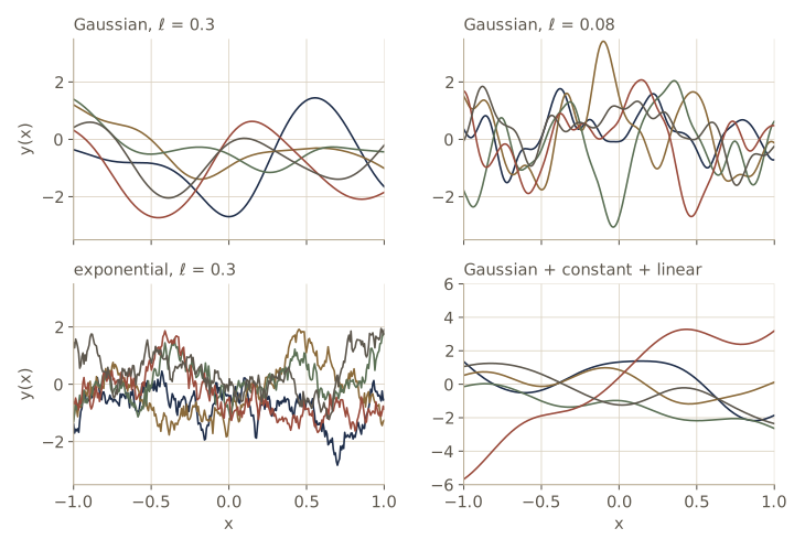
The choice of kernel is the choice of prior, and it matters. The Gaussian kernel’s samples are infinitely differentiable; the exponential kernel’s are continuous but nowhere smooth. Kernels encode what we believe about the function before seeing data: smoothness, typical amplitude (\(\theta_0\) is the prior variance of \(y(\mathbf{x})\)), how far correlations reach (\(\ell\)), trends, and so on.
Gaussian process regression
Now use a Gaussian process for regression. The observed targets are noisy function values,
\[t_n = y(\mathbf{x}_n) + \epsilon_n, \qquad p(t_n \mid y_n) = \mathcal{N}(t_n \mid y_n, \beta^{-1}),\]with independent noise of precision \(\beta\), so \(p(\mathbf{t} \mid \mathbf{y}) = \mathcal{N}(\mathbf{t} \mid \mathbf{y}, \beta^{-1} \mathbf{I}_N)\). The Gaussian process prior says \(p(\mathbf{y}) = \mathcal{N}(\mathbf{y} \mid \mathbf{0}, \mathbf{K})\). The targets are a sum of two independent zero-mean Gaussian vectors, so they are Gaussian with the covariances added (this is the marginalization formula for linear-Gaussian models from module 02):
\[p(\mathbf{t}) = \int p(\mathbf{t} \mid \mathbf{y})\, p(\mathbf{y})\, d\mathbf{y} = \mathcal{N}(\mathbf{t} \mid \mathbf{0}, \mathbf{C}_N), \qquad C(\mathbf{x}_n, \mathbf{x}_m) = k(\mathbf{x}_n, \mathbf{x}_m) + \beta^{-1} \delta_{nm}.\]Given training targets \(\mathbf{t} = (t_1, \dots, t_N)^{\mathrm{T}}\), we want the predictive distribution of \(t_{N+1}\) at a new input \(\mathbf{x}_{N+1}\) (the conditioning on all the inputs is left implicit). The vector \((t_1, \dots, t_N, t_{N+1})\) is again zero-mean Gaussian, with the \((N+1) \times (N+1)\) covariance matrix built the same way. Partition it as
\[\mathbf{C}_{N+1} = \begin{pmatrix} \mathbf{C}_N & \mathbf{k} \\ \mathbf{k}^{\mathrm{T}} & c \end{pmatrix}, \qquad k_n = k(\mathbf{x}_n, \mathbf{x}_{N+1}), \quad c = k(\mathbf{x}_{N+1}, \mathbf{x}_{N+1}) + \beta^{-1}.\]The conditional distribution of one block of a Gaussian vector given the other is Gaussian, with the mean and covariance formulas of module 02 (Bishop’s 2.81–2.82). With zero means they give:
Result. The Gaussian process predictive distribution is \(p(t_{N+1} \mid \mathbf{t}) = \mathcal{N}(t_{N+1} \mid m(\mathbf{x}_{N+1}), \sigma^2(\mathbf{x}_{N+1}))\) with
\[m(\mathbf{x}_{N+1}) = \mathbf{k}^{\mathrm{T}} \mathbf{C}_N^{-1} \mathbf{t}, \qquad \sigma^2(\mathbf{x}_{N+1}) = c - \mathbf{k}^{\mathrm{T}} \mathbf{C}_N^{-1} \mathbf{k}.\]
Both depend on the test input through \(\mathbf{k}\) and \(c\). The variance starts from the prior variance \(c\) and subtracts what the training data explain; far from the data \(\mathbf{k} \approx \mathbf{0}\) and we are back to the prior. The mean can be written \(m(\mathbf{x}) = \sum_n a_n k(\mathbf{x}_n, \mathbf{x})\) with \(\mathbf{a} = \mathbf{C}_N^{-1} \mathbf{t}\), a combination of kernel functions centered on the data, which for a radial kernel is a radial basis function expansion. And since \(\mathbf{C}_N = \mathbf{K} + \beta^{-1} \mathbf{I}\), it is exactly the kernel ridge regression prediction with \(\lambda = \beta^{-1}\): the Bayesian model supplies the error bars that the dual least-squares view lacked.
The prediction must be computed without forming \(\mathbf{C}_N^{-1}\). Factor \(\mathbf{C}_N = \mathbf{L} \mathbf{L}^{\mathrm{T}}\) once. Then \(\mathbf{a} = \mathbf{L}^{-\mathrm{T}} (\mathbf{L}^{-1} \mathbf{t})\) takes two triangular solves; with \(\mathbf{v} = \mathbf{L}^{-1} \mathbf{k}\) the variance is \(c - \mathbf{v}^{\mathrm{T}} \mathbf{v}\), since \(\mathbf{k}^{\mathrm{T}} \mathbf{C}_N^{-1} \mathbf{k} = \mathbf{k}^{\mathrm{T}} \mathbf{L}^{-\mathrm{T}} \mathbf{L}^{-1} \mathbf{k}\). Triangular solves are cheap and numerically stable, and the factor also gives \(\ln \lvert \mathbf{C}_N \rvert = 2 \sum_n \ln L_{nn}\), which we need shortly.
def kernel_diag(kernel, X):
    """Diagonal k(x, x) of a kernel at each row of X."""
    return np.array([kernel(X[i:i + 1], X[i:i + 1])[0, 0] for i in range(len(X))])

def gp_predict(X, t, X_new, kernel, beta):
    """GP regression: predictive mean and variance of t at the rows of X_new."""
    C = kernel(X, X) + np.eye(len(X)) / beta          # C_N = K + I / beta
    L = np.linalg.cholesky(C)
    a = solve_triangular(L.T, solve_triangular(L, t, lower=True), lower=False)  # C_N^-1 t
    k = kernel(X, X_new)                              # column j: k(x_n, x_new_j)
    mean = k.T @ a                                    # m = k^T C_N^-1 t
    v = solve_triangular(L, k, lower=True)            # v = L^-1 k
    c = kernel_diag(kernel, X_new) + 1 / beta
    var = c - np.sum(v**2, axis=0)                    # c - k^T C_N^-1 k
    return mean, var

# training data: 30 noisy points, then remove those in a gap between 0.45 and 0.7
X_all, t_all = make_sin_data(30, np.random.default_rng(2))
keep = (X_all[:, 0] < 0.45) | (X_all[:, 0] > 0.7)
X_gp, t_gp = X_all[keep], t_all[keep]
kern = lambda A, B: se_kernel(A, B, theta0=1.0, ell=0.2)
beta = 25.0                                       # noise standard deviation 0.2

X_show = np.array([[0.2], [0.57], [1.2]])
mean, var = gp_predict(X_gp, t_gp, X_show, kern, beta)
print(f"N = {len(t_gp)} training points")
for x, m, s in zip(X_show[:, 0], mean, np.sqrt(var)):
    print(f"x = {x:4.2f}:  mean {m:7.3f}   sd {s:.3f}   true {np.sin(2*np.pi*x):7.3f}")
N = 21 training points
x = 0.20:  mean   1.031   sd 0.218   true   0.951
x = 0.57:  mean  -0.583   sd 0.330   true  -0.426
x = 1.20:  mean   0.072   sd 0.816   true   0.951
At \(x = 0.2\), inside the data, the predictive standard deviation is barely above the noise level \(\beta^{-1/2} = 0.2\). In the gap it grows to 0.33, and at \(x = 1.2\), beyond the data, the mean has fallen back to about zero, the prior mean, while the standard deviation has grown to 0.82, on its way to the prior value \(\sqrt{\theta_0 + \beta^{-1}} \approx 1.02\). The GP does not pretend to know that the sine continues. For comparison, here is the same computation written as the formula reads, with an explicit inverse. We show it once to confirm the Cholesky version; the explicit inverse costs more and loses accuracy when \(\mathbf{C}_N\) is badly conditioned, so we avoid it everywhere else.
C_N = kern(X_gp, X_gp) + np.eye(len(t_gp)) / beta
C_inv = np.linalg.inv(C_N)
k = kern(X_gp, X_show)
mean_inv = k.T @ C_inv @ t_gp
var_inv = 1.0 + 1 / beta - np.sum(k * (C_inv @ k), axis=0)
print(f"max difference in mean {np.max(np.abs(mean_inv - mean)):.1e}, "
      f"in variance {np.max(np.abs(var_inv - var)):.1e}")

a_krr = ridge_dual(kern(X_gp, X_gp), t_gp, lam=1 / beta)   # kernel ridge, lambda = 1/beta
krr_diff = np.max(np.abs(k.T @ a_krr - mean))
print(f"GP mean vs kernel ridge prediction: max difference {krr_diff:.1e}")
max difference in mean 5.8e-15, in variance 1.1e-14
GP mean vs kernel ridge prediction: max difference 1.3e-15
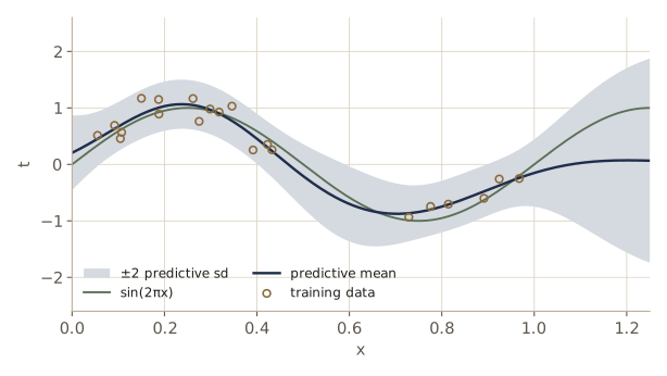
Note that our variance is the variance of a new target \(t_{N+1}\), noise included. For the variance of the underlying function value \(y(\mathbf{x}_{N+1})\), leave out the \(\beta^{-1}\) in \(c\). Near the data the difference is most of the variance.
Bayesian linear regression as a special case
If the kernel is built from \(M\) basis functions, \(k(\mathbf{x}, \mathbf{x}') = \alpha^{-1} \boldsymbol{\phi}(\mathbf{x})^{\mathrm{T}} \boldsymbol{\phi}(\mathbf{x}')\), the Gaussian process is the Bayesian linear regression model of module 03, and the two predictive distributions must agree. Module 03 gives the posterior \(\mathcal{N}(\mathbf{w} \mid \mathbf{m}_N, \mathbf{S}_N)\) with \(\mathbf{S}_N^{-1} = \alpha \mathbf{I} + \beta \mathbf{\Phi}^{\mathrm{T}} \mathbf{\Phi}\) and \(\mathbf{m}_N = \beta \mathbf{S}_N \mathbf{\Phi}^{\mathrm{T}} \mathbf{t}\), and the predictive mean \(\mathbf{m}_N^{\mathrm{T}} \boldsymbol{\phi}(\mathbf{x})\) and variance \(\beta^{-1} + \boldsymbol{\phi}(\mathbf{x})^{\mathrm{T}} \mathbf{S}_N \boldsymbol{\phi}(\mathbf{x})\). (The algebraic proof uses the matrix inversion identities of Appendix C; it is Bishop’s exercise 6.21.)
Phi_gp = gauss_basis(X_gp)
S_N_inv = alpha * np.eye(9) + beta * Phi_gp.T @ Phi_gp
m_N = beta * np.linalg.solve(S_N_inv, Phi_gp.T @ t_gp)
phi_show = gauss_basis(X_show)
blr_mean = phi_show @ m_N
blr_var = 1 / beta + np.sum(phi_show * np.linalg.solve(S_N_inv, phi_show.T).T, axis=1)

basis_kernel = lambda A, B: gauss_basis(A) @ gauss_basis(B).T / alpha
gp_mean, gp_var = gp_predict(X_gp, t_gp, X_show, basis_kernel, beta)
print("weight space  mean", blr_mean, "  var", blr_var)
print("function space mean", gp_mean, "  var", gp_var)
weight space  mean [ 1.0433 -0.5124 -0.0019]   var [0.0495 0.2065 0.0417]
function space mean [ 1.0433 -0.5124 -0.0019]   var [0.0495 0.2065 0.0417]
Same numbers from the two viewpoints. The weight-space view inverts an \(M \times M\) matrix, the function-space view an \(N \times N\) one. For a finite basis with \(M < N\) the weight-space view is cheaper; the function-space view is the one that allows kernels, like the Gaussian, that correspond to infinitely many basis functions.
The cost of exact inference
The Cholesky factorization of \(\mathbf{C}_N\) takes about \(N^3/3\) floating-point operations, so exact Gaussian process regression costs \(O(N^3)\) time and \(O(N^2)\) memory. It is done once per training set (and per hyperparameter setting). After that, each test point costs \(O(N)\) for the mean and \(O(N^2)\) for the variance. In theory, doubling \(N\) multiplies the factorization time by eight. Measured ratios are noisier, because of multithreading, caching, and whatever else the machine is doing (your times will differ), but the steep growth is plain.
X_big = np.random.default_rng(10).uniform(0, 1, (2000, 1))
previous = None
for N in [500, 1000, 2000]:
    C = se_kernel(X_big[:N], X_big[:N]) + 0.04 * np.eye(N)
    times = []
    for _ in range(3):                                        # best of three runs
        t0 = time.perf_counter()
        np.linalg.cholesky(C)
        times.append(time.perf_counter() - t0)
    ratio = "" if previous is None else f"   ({min(times) / previous:.1f} x previous N)"
    print(f"N = {N:4d}: Cholesky of C_N takes {min(times) * 1e3:6.1f} ms{ratio}")
    previous = min(times)
N =  500: Cholesky of C_N takes    2.3 ms
N = 1000: Cholesky of C_N takes   15.6 ms   (6.6 x previous N)
N = 2000: Cholesky of C_N takes   78.5 ms   (5.0 x previous N)
For tens of thousands of points this becomes the bottleneck, and many approximations have been developed that summarize the data with a smaller set of points or low-rank matrices; Bishop §6.4.2 points to the literature, and Rasmussen and Williams (2006, chapter 8) survey them. Gaussian process regression also extends to vector-valued targets (called co-kriging in geostatistics, where Gaussian process regression itself is known as kriging).
Learning the hyperparameters
Our predictions depended on \(\theta_0\), \(\ell\), and \(\beta\), which we simply chose. In practice we fix a parametric family of kernels and learn these hyperparameters \(\boldsymbol{\theta}\) from the data. The Gaussian process gives us the tool directly: the marginal likelihood \(p(\mathbf{t} \mid \boldsymbol{\theta}) = \mathcal{N}(\mathbf{t} \mid \mathbf{0}, \mathbf{C}_N(\boldsymbol{\theta}))\), in which the function values have already been integrated out. Maximizing it is type-2 maximum likelihood, the same idea as the evidence approximation of module 03. Its logarithm is
\[\ln p(\mathbf{t} \mid \boldsymbol{\theta}) = \underbrace{-\frac{1}{2} \mathbf{t}^{\mathrm{T}} \mathbf{C}_N^{-1} \mathbf{t}}_{\text{data fit}} \; \underbrace{- \frac{1}{2} \ln \lvert \mathbf{C}_N \rvert}_{\text{complexity penalty}} \; - \frac{N}{2} \ln (2\pi).\]The first term rewards covariances under which the targets are typical. The second penalizes covariance matrices that spread probability over many possible data sets (a flexible model has a large determinant). Their balance is an automatic Occam’s razor, as in module 03.
For gradient-based optimization we need the derivative with respect to each hyperparameter \(\theta_i\). Two identities from Bishop’s Appendix C do the work: \(\partial \mathbf{C}^{-1} / \partial \theta_i = -\mathbf{C}^{-1} (\partial \mathbf{C} / \partial \theta_i) \mathbf{C}^{-1}\) and \(\partial \ln \lvert \mathbf{C} \rvert / \partial \theta_i = \operatorname{Tr}(\mathbf{C}^{-1} \partial \mathbf{C} / \partial \theta_i)\). Applying them term by term, and writing \(\mathbf{a} = \mathbf{C}_N^{-1} \mathbf{t}\),
\[\begin{aligned} \frac{\partial}{\partial \theta_i} \ln p(\mathbf{t} \mid \boldsymbol{\theta}) &= \frac{1}{2} \mathbf{t}^{\mathrm{T}} \mathbf{C}_N^{-1} \frac{\partial \mathbf{C}_N}{\partial \theta_i} \mathbf{C}_N^{-1} \mathbf{t} - \frac{1}{2} \operatorname{Tr}\left( \mathbf{C}_N^{-1} \frac{\partial \mathbf{C}_N}{\partial \theta_i} \right) \\ &= \frac{1}{2} \operatorname{Tr}\left( \left( \mathbf{a} \mathbf{a}^{\mathrm{T}} - \mathbf{C}_N^{-1} \right) \frac{\partial \mathbf{C}_N}{\partial \theta_i} \right). \end{aligned}\]Hyperparameters must stay positive, so we optimize their logarithms: \(\ln \theta_0\), \(\ln \ell\), and \(\ln \sigma_n^2\), where \(\sigma_n^2 = \beta^{-1}\) is the noise variance. For the Gaussian kernel \(\mathbf{K}\) with entries \(\theta_0 \exp(-d_{nm} / 2\ell^2)\), where \(d_{nm} = \lVert \mathbf{x}_n - \mathbf{x}_m \rVert^2\), the derivatives are
\[\frac{\partial \mathbf{C}_N}{\partial \ln \theta_0} = \mathbf{K}, \qquad \frac{\partial C_{nm}}{\partial \ln \ell} = K_{nm} \frac{d_{nm}}{\ell^2}, \qquad \frac{\partial \mathbf{C}_N}{\partial \ln \sigma_n^2} = \sigma_n^2 \mathbf{I}.\]We check the gradient against finite differences before trusting it.
def gp_log_marginal(log_params, X, t, return_parts=False):
    """Log marginal likelihood of GP regression (Gaussian kernel) and its gradient.
    log_params = (ln theta0, ln ell, ln noise_variance)."""
    theta0, ell, noise_var = np.exp(log_params)
    N = len(t)
    D = sq_dists(X, X)
    K = theta0 * np.exp(-D / (2 * ell**2))
    C = K + noise_var * np.eye(N)
    L = np.linalg.cholesky(C)
    a = solve_triangular(L.T, solve_triangular(L, t, lower=True), lower=False)  # C^-1 t
    data_fit = -0.5 * t @ a
    complexity = -np.sum(np.log(np.diag(L)))          # -1/2 ln|C| = -sum ln L_nn
    lml = data_fit + complexity - 0.5 * N * np.log(2 * np.pi)
    if return_parts:
        return lml, data_fit, complexity
    C_inv = solve_triangular(L.T, solve_triangular(L, np.eye(N), lower=True))
    A = np.outer(a, a) - C_inv
    dC = [K, K * D / ell**2, noise_var * np.eye(N)]    # dC / d(log params)
    grad = np.array([0.5 * np.sum(A * dCi) for dCi in dC])   # 1/2 Tr(A dC)
    return lml, grad

p0 = np.log([1.0, 0.2, 0.04])
lml, grad = gp_log_marginal(p0, X_gp, t_gp)
eps = 1e-6
lml_at = lambda p: gp_log_marginal(p, X_gp, t_gp)[0]
fd = [(lml_at(p0 + eps * e) - lml_at(p0 - eps * e)) / (2 * eps) for e in np.eye(3)]
print(f"ln p(t) = {lml:.4f}")
print("analytic gradient:", grad)
print("finite differences:", np.array(fd))
ln p(t) = -3.0279
analytic gradient: [-1.7098  3.8956 -2.0097]
finite differences: [-1.7098  3.8956 -2.0097]
Now maximize. We hand the negative log marginal likelihood and our gradient to a generic quasi-Newton optimizer, scipy.optimize.minimize with L-BFGS-B, the kind of off-the-shelf method Bishop has in mind here; bounds on the log noise variance keep the matrix well conditioned. The log marginal likelihood is not concave in general and can have several local maxima, so we start from several length-scales.
def fit_gp_hyperparameters(X, t, starts):
    """Maximize the log marginal likelihood from several starts (L-BFGS-B)."""
    neg = lambda p: tuple(-v for v in gp_log_marginal(p, X, t))
    bounds = [(-6, 6), (-6, 4), (np.log(1e-6), 2)]
    results = []
    for start in starts:
        res = minimize(neg, np.log(start), jac=True, method="L-BFGS-B", bounds=bounds)
        results.append((-res.fun, np.exp(res.x)))
        theta0, ell, noise_var = np.exp(res.x)
        print(f"start ell = {start[1]:5.2f}:  ln p(t) = {-res.fun:8.3f}   "
              f"theta0 = {theta0:.3f}   ell = {ell:.3f}   noise sd = {np.sqrt(noise_var):.3f}")
    return max(results, key=lambda r: r[0])

starts = [(1.0, 0.03, 0.04), (1.0, 0.3, 0.04), (1.0, 3.0, 0.04)]   # (theta0, ell, noise)
best_lml, best_params = fit_gp_hyperparameters(X_gp, t_gp, starts)
start ell =  0.03:  ln p(t) =   -1.782   theta0 = 0.485   ell = 0.220   noise sd = 0.170
start ell =  0.30:  ln p(t) =   -1.782   theta0 = 0.485   ell = 0.220   noise sd = 0.170
start ell =  3.00:  ln p(t) =   -1.782   theta0 = 0.485   ell = 0.220   noise sd = 0.170
All three starts reach the same maximum here. The fitted noise standard deviation, 0.17, is close to the 0.2 we used to generate the data; the amplitude \(\theta_0 \approx 0.49\) is close to the variance of \(\sin(2\pi x)\) over a period, which is 1/2; and the length-scale 0.22 is a sensible scale for one period of a sine. To see what the marginal likelihood is trading off, keep \(\theta_0\) and the noise at their fitted values and change only the length-scale: a short one (a flexible model), the optimum, and a long one (a stiff model).
theta0_ml, ell_ml, noise_ml = best_params
settings = {                        # vary ell only; theta0 and noise stay at fitted values
    "short length-scale": (theta0_ml, 0.03, noise_ml),
    "maximum likelihood": (theta0_ml, ell_ml, noise_ml),
    "long length-scale": (theta0_ml, 1.0, noise_ml),
}
print(f"{'setting':20s} {'ell':>6s} {'data fit':>9s} {'-1/2 ln|C|':>11s} {'ln p(t)':>9s}")
for name, (th0, ell, nv) in settings.items():
    lml, fit, comp = gp_log_marginal(np.log([th0, ell, nv]), X_gp, t_gp, True)
    print(f"{name:20s} {ell:6.3f} {fit:9.2f} {comp:11.2f} {lml:9.2f}")
setting                 ell  data fit  -1/2 ln|C|   ln p(t)
short length-scale    0.030     -8.12       13.68    -13.73
maximum likelihood    0.220    -10.50       28.02     -1.78
long length-scale     1.000    -50.63       32.39    -37.53
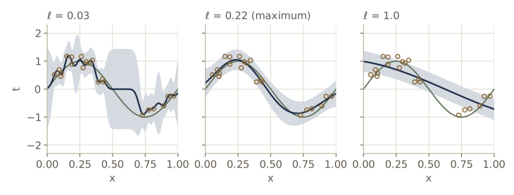
Read the table from top to bottom. The data-fit term gets worse as the model stiffens, from −8.1 to −10.5 to −50.6: a flexible model can make the observed targets typical. The term \(-\frac{1}{2} \ln \lvert \mathbf{C}_N \rvert\) moves the other way, from 13.7 to 28.0 to 32.4, because a flexible model spreads its probability over many possible data sets and so has a larger determinant. The sum peaks at the maximum likelihood length-scale, well above both neighbors.
A fully Bayesian treatment would put a prior on \(\boldsymbol{\theta}\) and integrate over it rather than optimize; that integral is intractable and needs the approximations of modules 10 and 11. Another extension lets the noise vary with the input (heteroscedastic noise), for instance by modeling \(\ln \beta(\mathbf{x})\) with a second Gaussian process.
Automatic relevance determination
A single length-scale treats all input directions alike. Give each input dimension its own:
\[k(\mathbf{x}, \mathbf{x}') = \theta_0 \exp\left( -\frac{1}{2} \sum_{i=1}^{D} \eta_i (x_i - x_i')^2 \right), \qquad \eta_i = 1/\ell_i^2.\]If \(\eta_i\) is small (\(\ell_i\) large), the kernel hardly changes as \(x_i\) changes, so functions drawn from the prior are nearly constant along that direction. Learning the \(\eta_i\) by maximizing the marginal likelihood therefore tells us which inputs matter: an input that does not help predict the target drives its \(\eta_i\) toward zero. This is automatic relevance determination (ARD), an idea first developed for Bayesian neural networks; the mechanism is analyzed in module 07’s relevance vector machine. The ARD kernel can be combined with constant and linear terms (Bishop’s 6.72) in the same way as before.
Our test: 100 points with two inputs uniform on the unit square, where the target depends only on the first, \(t = \sin(2\pi x_1) + \epsilon\) with noise standard deviation 0.1. The gradient generalizes directly: \(\partial C_{nm} / \partial \ln \ell_i = K_{nm} (x_{ni} - x_{mi})^2 / \ell_i^2\). We cap \(\ell_i\) at \(e^7 \approx 1100\), far beyond the size of the input box.
def ard_log_marginal(log_params, X, t):
    """Log marginal likelihood and gradient for a GP with an ARD Gaussian kernel.
    log_params = (ln theta0, ln ell_1, ..., ln ell_D, ln noise_variance)."""
    N, D = X.shape
    theta0, noise_var = np.exp(log_params[0]), np.exp(log_params[-1])
    ells = np.exp(log_params[1:-1])
    Dsq = [(X[:, [i]] - X[:, [i]].T) ** 2 for i in range(D)]   # squared differences, input i
    K = theta0 * np.exp(-0.5 * sum(Dsq[i] / ells[i]**2 for i in range(D)))
    C = K + noise_var * np.eye(N)
    L = np.linalg.cholesky(C)
    a = solve_triangular(L.T, solve_triangular(L, t, lower=True), lower=False)
    lml = -0.5 * t @ a - np.sum(np.log(np.diag(L))) - 0.5 * N * np.log(2 * np.pi)
    C_inv = solve_triangular(L.T, solve_triangular(L, np.eye(N), lower=True))
    A = np.outer(a, a) - C_inv
    dC = [K] + [K * Dsq[i] / ells[i]**2 for i in range(D)] + [noise_var * np.eye(N)]
    return lml, np.array([0.5 * np.sum(A * dCi) for dCi in dC])

rng_ard = np.random.default_rng(7)
X_ard = rng_ard.uniform(0, 1, (100, 2))
t_ard = np.sin(2 * np.pi * X_ard[:, 0]) + 0.1 * rng_ard.standard_normal(100)

path = []                                    # the optimizer's iterates, for the figure
res = minimize(lambda p: tuple(-v for v in ard_log_marginal(p, X_ard, t_ard)),
               np.log([1.0, 1.0, 1.0, 0.1]), jac=True, method="L-BFGS-B",
               bounds=[(-5, 5), (-5, 7), (-5, 7), (np.log(1e-6), 2)],
               callback=lambda p: path.append(np.exp(p)))
theta0, ell1, ell2, nv = np.exp(res.x)
print(f"{res.nit} iterations, ln p(t) = {-res.fun:.2f}")
print(f"ell_1 = {ell1:.3f}  (eta_1 = {1 / ell1**2:.2f})")
print(f"ell_2 = {ell2:.1f}  (eta_2 = {1 / ell2**2:.1e})")
print(f"theta0 = {theta0:.2f}, noise sd = {np.sqrt(nv):.3f}")
for it in [0, 4, 9, len(path) - 1]:
    print(f"  after iteration {it + 1:2d}: ell_1 = {path[it][1]:6.3f}   "
          f"ell_2 = {path[it][2]:8.2f}")
25 iterations, ln p(t) = 67.70
ell_1 = 0.390  (eta_1 = 6.58)
ell_2 = 1096.6  (eta_2 = 8.3e-07)
theta0 = 3.52, noise sd = 0.102
  after iteration  1: ell_1 =  0.305   ell_2 =     2.48
  after iteration  5: ell_1 =  0.254   ell_2 =     2.42
  after iteration 10: ell_1 =  0.329   ell_2 =    56.97
  after iteration 25: ell_1 =  0.390   ell_2 =  1096.63
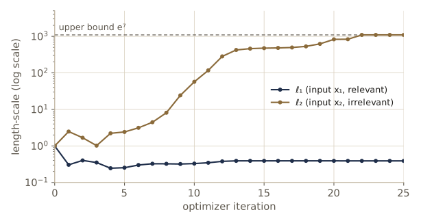
For comparison, fit the same data with the isotropic kernel of the previous section, which has to use one length-scale for both inputs.
iso_lml, iso_params = fit_gp_hyperparameters(X_ard, t_ard, [(1.0, 0.3, 0.01)])
print(f"ARD ln p(t) = {-res.fun:.2f}  vs  isotropic ln p(t) = {iso_lml:.2f}")
start ell =  0.30:  ln p(t) =   42.311   theta0 = 1.741   ell = 0.388   noise sd = 0.102
ARD ln p(t) = 67.70  vs  isotropic ln p(t) = 42.31
The isotropic kernel compromises on a length-scale suited to \(x_1\), which makes it wrongly sensitive to \(x_2\), and its marginal likelihood is far lower. With ARD the fitted model depends on \(x_2\) so weakly that we could drop that input.
In practice, ARD length-scales are only comparable if the inputs are on similar scales, so standardize inputs first. And a large learned length-scale says that an input is not needed given the others: two strongly correlated inputs may share the relevance between them in ways that depend on the starting point.
Gaussian processes for classification
For two-class classification with targets \(t \in \{0, 1\}\) we want \(p(t = 1 \mid \mathbf{x})\), a number in \((0, 1)\), while a Gaussian process produces values on the whole real line. The fix is the one used by logistic regression in module 04: put a Gaussian process prior on a latent function \(a(\mathbf{x})\) and pass it through the logistic sigmoid, \(y = \sigma(a)\). Then
\[p(t \mid a) = \sigma(a)^{t} \left(1 - \sigma(a)\right)^{1 - t}.\]For the training inputs collect \(\mathbf{a}_N = (a(\mathbf{x}_1), \dots, a(\mathbf{x}_N))^{\mathrm{T}}\), and add the test input to get \(\mathbf{a}_{N+1}\). The prior is \(p(\mathbf{a}_{N+1}) = \mathcal{N}(\mathbf{a}_{N+1} \mid \mathbf{0}, \mathbf{C}_{N+1})\) with
\[C(\mathbf{x}_n, \mathbf{x}_m) = k(\mathbf{x}_n, \mathbf{x}_m) + \nu \, \delta_{nm}.\]There is no observation noise on \(a\) (the labels are assumed correct and the randomness is in the Bernoulli draw), so \(\nu\) is only a small fixed jitter that keeps \(\mathbf{C}\) positive definite. The prediction we want is
\[p(t_{N+1} = 1 \mid \mathbf{t}_N) = \int \sigma(a_{N+1}) \, p(a_{N+1} \mid \mathbf{t}_N) \, da_{N+1}.\]Unlike regression, the posterior over the latent values is not Gaussian, because the likelihood is a product of sigmoids, and this integral has no closed form. It can be estimated by sampling (module 11), or we can approximate the posterior by a Gaussian. Three ways to find that Gaussian are in common use: variational inference with a local bound on the sigmoid and expectation propagation (both in module 10), and the Laplace approximation, which we now develop in full.
The Laplace approximation
Recall from module 04 that the Laplace approximation replaces a distribution by the Gaussian centered at its mode, with precision equal to the negative Hessian of the log density there.
Splitting the problem. The latent value at the test point is linked to the data only through the training latents, so
\[p(a_{N+1} \mid \mathbf{t}_N) = \int p(a_{N+1} \mid \mathbf{a}_N) \, p(\mathbf{a}_N \mid \mathbf{t}_N) \, d\mathbf{a}_N.\]The first factor is the noise-free Gaussian process conditional, from the same partition as in regression,
\[p(a_{N+1} \mid \mathbf{a}_N) = \mathcal{N}\left(a_{N+1} \mid \mathbf{k}^{\mathrm{T}} \mathbf{C}_N^{-1} \mathbf{a}_N, \; c - \mathbf{k}^{\mathrm{T}} \mathbf{C}_N^{-1} \mathbf{k}\right),\]now with \(c = k(\mathbf{x}_{N+1}, \mathbf{x}_{N+1}) + \nu\). So we need a Gaussian approximation of the posterior \(p(\mathbf{a}_N \mid \mathbf{t}_N)\); the integral is then a linear-Gaussian marginal.
The log posterior. Using \(\ln \sigma(a) = a - \ln(1 + e^{a})\) and \(\ln(1 - \sigma(a)) = -\ln(1 + e^{a})\), the log-likelihood of one label is \(t_n a_n - \ln(1 + e^{a_n})\). Up to a constant, the log posterior is
\[\begin{aligned} \Psi(\mathbf{a}_N) &= \ln p(\mathbf{a}_N) + \ln p(\mathbf{t}_N \mid \mathbf{a}_N) \\ &= -\frac{1}{2} \mathbf{a}_N^{\mathrm{T}} \mathbf{C}_N^{-1} \mathbf{a}_N - \frac{1}{2} \ln \lvert \mathbf{C}_N \rvert - \frac{N}{2} \ln(2\pi) \\ &\qquad + \mathbf{t}_N^{\mathrm{T}} \mathbf{a}_N - \sum_{n=1}^{N} \ln(1 + e^{a_n}). \end{aligned}\]Using \(d \ln(1 + e^{a}) / da = \sigma(a)\) and \(d\sigma / da = \sigma(1 - \sigma)\), its gradient and Hessian are
\[\nabla \Psi = \mathbf{t}_N - \boldsymbol{\sigma}_N - \mathbf{C}_N^{-1} \mathbf{a}_N, \qquad \nabla \nabla \Psi = -\mathbf{W}_N - \mathbf{C}_N^{-1},\]where \(\boldsymbol{\sigma}_N\) has elements \(\sigma(a_n)\) and \(\mathbf{W}_N\) is diagonal with elements \(\sigma(a_n)(1 - \sigma(a_n))\), all in \((0, 1/4]\). Both \(\mathbf{W}_N\) and \(\mathbf{C}_N^{-1}\) are positive definite, so the Hessian is negative definite everywhere: \(\Psi\) is strictly concave and has a single maximum. (The posterior is still not Gaussian, since the Hessian changes with \(\mathbf{a}_N\).)
Newton’s method for the mode. Setting the gradient to zero gives a nonlinear equation, so we iterate Newton steps, \(\mathbf{a}^{\text{new}} = \mathbf{a} - (\nabla \nabla \Psi)^{-1} \nabla \Psi\), exactly as IRLS did for logistic regression in module 04. Dropping the subscript \(N\) for the moment:
\[\begin{aligned} \mathbf{a}^{\text{new}} &= \mathbf{a} + (\mathbf{W} + \mathbf{C}^{-1})^{-1} (\mathbf{t} - \boldsymbol{\sigma} - \mathbf{C}^{-1} \mathbf{a}) \\ &= (\mathbf{W} + \mathbf{C}^{-1})^{-1} \left[ (\mathbf{W} + \mathbf{C}^{-1}) \mathbf{a} + \mathbf{t} - \boldsymbol{\sigma} - \mathbf{C}^{-1} \mathbf{a} \right] \\ &= (\mathbf{W} + \mathbf{C}^{-1})^{-1} (\mathbf{t} - \boldsymbol{\sigma} + \mathbf{W} \mathbf{a}) \\ &= \mathbf{C} (\mathbf{I} + \mathbf{W} \mathbf{C})^{-1} (\mathbf{t} - \boldsymbol{\sigma} + \mathbf{W} \mathbf{a}), \end{aligned}\]where the last line uses \((\mathbf{W} + \mathbf{C}^{-1})^{-1} = [\mathbf{C}^{-1} (\mathbf{C} \mathbf{W} + \mathbf{I})]^{-1} = (\mathbf{I} + \mathbf{C} \mathbf{W})^{-1} \mathbf{C} = \mathbf{C} (\mathbf{I} + \mathbf{W} \mathbf{C})^{-1}\) (the push-through identity again), which avoids inverting \(\mathbf{C}\). At the mode \(\hat{\mathbf{a}}_N\) the gradient vanishes, so
\[\hat{\mathbf{a}}_N = \mathbf{C}_N (\mathbf{t}_N - \hat{\boldsymbol{\sigma}}_N),\]and the Laplace approximation is \(q(\mathbf{a}_N) = \mathcal{N}(\mathbf{a}_N \mid \hat{\mathbf{a}}_N, \mathbf{H}^{-1})\) with \(\mathbf{H} = \mathbf{W}_N + \mathbf{C}_N^{-1}\) evaluated at the mode.
The predictive distribution. Plug \(q\) into the integral. The marginal of a linear-Gaussian model (module 02) has mean \(\mathbf{k}^{\mathrm{T}} \mathbf{C}_N^{-1} \hat{\mathbf{a}}_N\) and variance \(c - \mathbf{k}^{\mathrm{T}} \mathbf{C}_N^{-1} \mathbf{k} + \mathbf{k}^{\mathrm{T}} \mathbf{C}_N^{-1} \mathbf{H}^{-1} \mathbf{C}_N^{-1} \mathbf{k}\). Using the mode condition for the mean, and the Woodbury identity \((\mathbf{C}_N + \mathbf{W}_N^{-1})^{-1} = \mathbf{C}_N^{-1} - \mathbf{C}_N^{-1} (\mathbf{W}_N + \mathbf{C}_N^{-1})^{-1} \mathbf{C}_N^{-1}\) for the variance:
Result. Under the Laplace approximation, \(p(a_{N+1} \mid \mathbf{t}_N) \approx \mathcal{N}(a_{N+1} \mid \mu_a, s_a^2)\) with
\[\mu_a = \mathbf{k}^{\mathrm{T}} (\mathbf{t}_N - \hat{\boldsymbol{\sigma}}_N), \qquad s_a^2 = c - \mathbf{k}^{\mathrm{T}} (\mathbf{W}_N^{-1} + \mathbf{C}_N)^{-1} \mathbf{k},\]and \(p(t_{N+1} = 1 \mid \mathbf{t}_N) \approx \sigma(\kappa(s_a^2) \, \mu_a)\) with \(\kappa(s^2) = (1 + \pi s^2 / 8)^{-1/2}\).
The last step is the probit approximation of the sigmoid-Gaussian integral from module 04 (Bishop §4.5.2). The mean formula has a nice reading: a training point with \(\hat{\sigma}_n \approx t_n\) (confidently classified) contributes almost nothing to predictions. For the decision boundary \(p = 0.5\) only the sign of \(\mu_a\) matters, since \(\kappa > 0\).
One numerical detail: \(\mathbf{W}_N^{-1}\) blows up when some \(\hat{\sigma}_n\) is near 0 or 1. Writing \((\mathbf{W}^{-1} + \mathbf{C})^{-1} = \mathbf{W}^{1/2} \mathbf{B}^{-1} \mathbf{W}^{1/2}\) with \(\mathbf{B} = \mathbf{I} + \mathbf{W}^{1/2} \mathbf{C} \mathbf{W}^{1/2}\) avoids the problem; \(\mathbf{B}\) is symmetric, well conditioned (its eigenvalues are at least 1), and has a Cholesky factor. Rasmussen and Williams (2006, §3.4) base their implementation of the Laplace approximation on \(\mathbf{B}\).
Our data: two classes in the plane, each a mixture of two Gaussian blobs (so a linear boundary cannot separate them), 50 points per class. Because we know how the data were generated, we can also compute the best possible (Bayes-optimal) classifier and compare.
MEANS = {0: np.array([[-1.0, 0.8], [1.0, -1.0]]),     # class 0: two blobs
         1: np.array([[0.2, -0.2], [-1.2, -1.2]])}     # class 1: two blobs
S_BLOB = 0.45                                         # standard deviation of every blob

def sample_two_class(n_per_class, rng):
    """Each class is an equal mixture of two isotropic Gaussians. Returns X, t."""
    X, t = [], []
    for c in (0, 1):
        comp = rng.integers(0, 2, n_per_class)
        X.append(MEANS[c][comp] + S_BLOB * rng.standard_normal((n_per_class, 2)))
        t.append(np.full(n_per_class, float(c)))
    return np.vstack(X), np.concatenate(t)

def bayes_optimal_prob(X):
    """True p(t = 1 | x) for the generating mixtures (equal class priors)."""
    dens = [sum(np.exp(-np.sum((X - m)**2, axis=1) / (2 * S_BLOB**2)) for m in MEANS[c])
            for c in (0, 1)]
    return dens[1] / (dens[0] + dens[1])

X_cls, t_cls = sample_two_class(50, np.random.default_rng(11))
X_test, t_test = sample_two_class(2000, np.random.default_rng(12))
print(X_cls.shape, "class counts:", np.bincount(t_cls.astype(int)))
bayes_acc = np.mean((bayes_optimal_prob(X_test) > 0.5) == t_test)
print(f"Bayes-optimal test accuracy: {bayes_acc:.3f}")
(100, 2) class counts: [50 50]
Bayes-optimal test accuracy: 0.920
Now the Newton iteration. We track \(\Psi\) (without its constant) and the size of the gradient, which should go to zero quadratically fast near the mode.
def log_posterior(a, C, t):
    """Psi(a) up to its constant: -1/2 a^T C^{-1} a + t^T a - sum ln(1 + e^a)."""
    return -0.5 * a @ np.linalg.solve(C, a) + t @ a - np.sum(np.logaddexp(0, a))

def laplace_mode(C, t, max_iter=50, tol=1e-6, verbose=False):
    """Newton's method for the mode of p(a | t), GP classification (Bishop's 6.83)."""
    N = len(t)
    a = np.zeros(N)
    for it in range(max_iter):
        s = expit(a)
        W = s * (1 - s)
        # a_new = C (I + W C)^-1 (t - sigma + W a)
        a_new = C @ np.linalg.solve(np.eye(N) + W[:, None] * C, t - s + W * a)
        step = np.max(np.abs(a_new - a))
        a = a_new
        if verbose:
            grad = t - expit(a) - np.linalg.solve(C, a)
            print(f"  iteration {it + 1}: Psi = {log_posterior(a, C, t):9.4f}   "
                  f"max |gradient| = {np.max(np.abs(grad)):.1e}")
        if step < tol:
            break
    return a

nu = 1e-6
theta0_c, ell_c = 16.0, 1.0
C_cls = se_kernel(X_cls, X_cls, theta0_c, ell_c) + nu * np.eye(len(t_cls))
a_hat = laplace_mode(C_cls, t_cls, verbose=True)
gap = np.max(np.abs(a_hat - C_cls @ (t_cls - expit(a_hat))))
print(f"mode condition: max |a_hat - C (t - sigma)| = {gap:.1e}")
  iteration 1: Psi =  -21.3835   max |gradient| = 1.9e-01
  iteration 2: Psi =  -15.4265   max |gradient| = 6.8e-02
  iteration 3: Psi =  -14.3252   max |gradient| = 2.1e-02
  iteration 4: Psi =  -14.2450   max |gradient| = 1.6e-03
  iteration 5: Psi =  -14.2443   max |gradient| = 2.8e-05
  iteration 6: Psi =  -14.2443   max |gradient| = 1.0e-08
  iteration 7: Psi =  -14.2443   max |gradient| = 1.0e-08
mode condition: max |a_hat - C (t - sigma)| = 5.0e-13
Starting from \(\mathbf{a} = \mathbf{0}\), the largest gradient component is 0.19 after one Newton step and \(3 \times 10^{-5}\) after five, and one more step reaches \(10^{-8}\), the floor set by rounding (computing \(\mathbf{C}_N^{-1} \mathbf{a}\) with a jitter of \(10^{-6}\) is not very accurate). The log posterior \(\Psi\) increases at every step and levels off at −14.2443. Next the predictive probabilities, using the \(\mathbf{B}\) form for the variance. We also check the probit approximation against the integral \(\int \sigma(a) \mathcal{N}(a \mid \mu_a, s_a^2)\, da\) computed by Gauss–Hermite quadrature.
def gp_classify(X, t, X_new, kernel, nu=1e-6):
    """Laplace GP classifier: latent mean and variance, and p(t = 1 | x)."""
    N = len(t)
    C = kernel(X, X) + nu * np.eye(N)
    a_hat = laplace_mode(C, t)
    s = expit(a_hat)
    sqrt_W = np.sqrt(s * (1 - s))
    B = np.eye(N) + sqrt_W[:, None] * C * sqrt_W[None, :]    # I + W^1/2 C W^1/2
    L_B = np.linalg.cholesky(B)
    k = kernel(X, X_new)
    mu_a = k.T @ (t - s)                                     # 6.87
    v = solve_triangular(L_B, sqrt_W[:, None] * k, lower=True)
    var_a = kernel_diag(kernel, X_new) + nu - np.sum(v**2, axis=0)    # 6.88 via B
    kappa = 1 / np.sqrt(1 + np.pi * var_a / 8)
    return mu_a, var_a, expit(kappa * mu_a)

kern_c = lambda A, B: se_kernel(A, B, theta0_c, ell_c)
X_q = np.array([[0.2, -0.2], [-0.1, 0.4], [3.0, 3.0]])
mu_a, var_a, p1 = gp_classify(X_cls, t_cls, X_q, kern_c)
nodes, weights = np.polynomial.hermite.hermgauss(60)    # for integrals of f(a) e^(-a^2)
for x, m, v, p in zip(X_q, mu_a, var_a, p1):
    exact = np.sum(weights * expit(m + np.sqrt(2 * v) * nodes)) / np.sqrt(np.pi)
    print(f"x = {x}:  mu_a = {m:6.2f}  s_a = {np.sqrt(v):5.2f}   "
          f"probit approx {p:.3f}   quadrature {exact:.3f}")
x = [ 0.2 -0.2]:  mu_a =   2.82  s_a =  0.87   probit approx 0.922   quadrature 0.925
x = [-0.1  0.4]:  mu_a =   3.36  s_a =  1.29   probit approx 0.932   quadrature 0.937
x = [3. 3.]:  mu_a =   0.00  s_a =  4.00   probit approx 0.500   quadrature 0.500
The probit approximation is accurate to about two decimal places. The third test point is far from all the data: its latent mean is near zero and its latent variance is back at the prior value \(\theta_0 = 16\), so the classifier says “probability 0.5” rather than extrapolating a confident label. A plain logistic regression would not do that.
Choosing the hyperparameters. The marginal likelihood \(p(\mathbf{t}_N \mid \boldsymbol{\theta}) = \int p(\mathbf{t}_N \mid \mathbf{a}_N) p(\mathbf{a}_N \mid \boldsymbol{\theta})\, d\mathbf{a}_N\) is again intractable, and the Laplace approximation of an integral (module 04) gives
\[\ln p(\mathbf{t}_N \mid \boldsymbol{\theta}) \approx \Psi(\hat{\mathbf{a}}_N) - \frac{1}{2} \ln \lvert \mathbf{W}_N + \mathbf{C}_N^{-1} \rvert + \frac{N}{2} \ln(2\pi).\]Two simplifications make this easy to compute. The \(-\frac{1}{2} \ln \lvert \mathbf{C}_N \rvert\) inside \(\Psi\) combines with the determinant term into \(-\frac{1}{2} \ln \lvert \mathbf{I} + \mathbf{C}_N \mathbf{W}_N \rvert = -\frac{1}{2} \ln \lvert \mathbf{B} \rvert\), and at the mode \(\mathbf{C}_N^{-1} \hat{\mathbf{a}}_N = \mathbf{t}_N - \hat{\boldsymbol{\sigma}}_N\). So
\[\ln p(\mathbf{t}_N \mid \boldsymbol{\theta}) \approx -\frac{1}{2} \hat{\mathbf{a}}_N^{\mathrm{T}} (\mathbf{t}_N - \hat{\boldsymbol{\sigma}}_N) + \mathbf{t}_N^{\mathrm{T}} \hat{\mathbf{a}}_N - \sum_n \ln(1 + e^{\hat{a}_n}) - \frac{1}{2} \ln \lvert \mathbf{B} \rvert.\]Its gradient is more involved than in regression, because the mode \(\hat{\mathbf{a}}_N\) itself moves when \(\boldsymbol{\theta}\) changes (Bishop’s 6.91–6.94 work it out). With only two hyperparameters we compare settings on a grid instead.
def laplace_log_marginal(C, t):
    """Laplace approximation to ln p(t | theta) for GP classification."""
    a = laplace_mode(C, t)
    s = expit(a)
    sqrt_W = np.sqrt(s * (1 - s))
    L_B = np.linalg.cholesky(np.eye(len(t)) + sqrt_W[:, None] * C * sqrt_W[None, :])
    log_det_B = 2 * np.sum(np.log(np.diag(L_B)))
    return -0.5 * a @ (t - s) + t @ a - np.sum(np.logaddexp(0, a)) - 0.5 * log_det_B

theta0_grid, ell_grid = [1.0, 4.0, 16.0, 64.0, 256.0], [0.25, 0.5, 1.0, 2.0]
C_of = lambda th0, l: se_kernel(X_cls, X_cls, th0, l) + nu * np.eye(len(t_cls))
table = np.array([[laplace_log_marginal(C_of(th0, l), t_cls) for l in ell_grid]
                  for th0 in theta0_grid])
print("rows theta0 =", theta0_grid, " columns ell =", ell_grid)
print(table)
i, j = np.unravel_index(np.argmax(table), table.shape)
best_theta0, best_ell = theta0_grid[i], ell_grid[j]
best_kernel = lambda A, B: se_kernel(A, B, best_theta0, best_ell)
_, _, p_test = gp_classify(X_cls, t_cls, X_test, best_kernel)
test_acc = np.mean((p_test > 0.5) == t_test)
print(f"best: theta0 = {best_theta0}, ell = {best_ell}; test accuracy {test_acc:.3f}")
rows theta0 = [1.0, 4.0, 16.0, 64.0, 256.0]  columns ell = [0.25, 0.5, 1.0, 2.0]
[[-53.3269 -40.9997 -39.2723 -53.0879]
 [-45.187  -31.0126 -28.2178 -41.4073]
 [-42.0613 -26.9291 -22.5995 -31.1348]
 [-43.4625 -27.3901 -21.196  -24.7915]
 [-46.7642 -30.3486 -22.1966 -22.3635]]
best: theta0 = 64.0, ell = 1.0; test accuracy 0.884
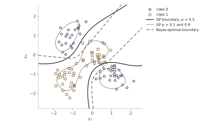
The approximate marginal likelihood peaks at \(\theta_0 = 64\) and \(\ell = 1\), inside the grid. The resulting boundary tracks the Bayes-optimal one where there are data and departs from it in the empty corners. Its test accuracy, 0.884, is about three and a half points below the best achievable 0.920, from only 100 training points. Multi-class problems use a softmax in place of the sigmoid, and the Laplace machinery carries over (Bishop §6.4.6 gives the reference).
Watch out. The Newton iteration and every prediction need linear solves with \(N \times N\) matrices, so Gaussian process classification has the same \(O(N^3)\) cost as regression, paid once per Newton step and per hyperparameter setting. And the Laplace approximation is centered at the mode: when the posterior is strongly skewed (for instance on nearly separable data with a large \(\theta_0\)) it can misjudge the latent variance, which expectation propagation (module 10) handles better.
Connection to neural networks
Module 05 showed that a two-layer network with enough hidden units can approximate any reasonable function, and that with maximum likelihood the number of hidden units \(M\) must be limited to avoid overfitting. From a Bayesian point of view there is no reason to limit \(M\); the prior controls complexity instead. So what happens as \(M \to \infty\)?
Neal (1996) showed that for a broad class of weight priors, with the output weights’ prior variance scaled like \(1/M\), the prior over network functions tends to a Gaussian process. The reason is the central limit theorem: the output \(y(\mathbf{x}) = \sum_{j=1}^{M} v_j h(\mathbf{u}_j^{\mathrm{T}} \mathbf{x} + b_j)\) is a sum of \(M\) independent, identically distributed terms, so its values at any finite set of inputs become jointly Gaussian. We can watch it happen: draw many random one-hidden-layer \(\tanh\) networks and look at the distribution of the output at a fixed input. A Gaussian has excess kurtosis 0.
def random_tanh_nets(x, M, n_nets, rng):
    """Outputs at inputs x of n_nets random nets: v ~ N(0, 1/M), u, b ~ N(0, 1)."""
    u = rng.standard_normal((n_nets, M, 1))
    b = rng.standard_normal((n_nets, M, 1))
    v = rng.standard_normal((n_nets, 1, M)) / np.sqrt(M)
    return (v @ np.tanh(u * x[None, None, :] + b))[:, 0, :]      # (n_nets, len(x))

x_nn = np.array([-0.5, 0.5])
for M in [1, 3, 30, 300]:
    Y = random_tanh_nets(x_nn, M, 20000, np.random.default_rng(13))
    z = (Y[:, 1] - Y[:, 1].mean()) / Y[:, 1].std()
    print(f"M = {M:3d}: excess kurtosis of y(0.5) = {np.mean(z**4) - 3:6.2f}   "
          f"cov[y(-0.5), y(0.5)] = {np.cov(Y.T)[0, 1]:.3f}")
M =   1: excess kurtosis of y(0.5) =   1.64   cov[y(-0.5), y(0.5)] = 0.246
M =   3: excess kurtosis of y(0.5) =   0.65   cov[y(-0.5), y(0.5)] = 0.243
M =  30: excess kurtosis of y(0.5) =   0.03   cov[y(-0.5), y(0.5)] = 0.248
M = 300: excess kurtosis of y(0.5) =   0.03   cov[y(-0.5), y(0.5)] = 0.243
The covariance between the outputs at two inputs is the same for every \(M\), about 0.24 up to sampling error: the \(1/M\) scaling of the output weights’ variance was chosen to make it so, and that covariance is the kernel of the limiting Gaussian process. What changes with \(M\) is the shape of the distribution. With one hidden unit the excess kurtosis is 1.6, far from Gaussian; with three it is 0.65; from thirty units on it is about 0.03, indistinguishable from zero with 20,000 sampled networks. Williams (1998) computed such kernels in closed form for some activation functions. They are not stationary (they cannot be written as a function of \(\mathbf{x} - \mathbf{x}'\)), because a zero-centered prior on the biases and input weights singles out the origin.
The limit has a cost. In a finite network, several outputs share the same hidden units, so what one output learns shapes the features used by the others. In the Gaussian process limit the outputs become independent, and that sharing is lost. Working with the kernel also integrates out the weights analytically, but the hyperparameters of the weight prior (which set the length-scales of the functions) still have to be learned, by the methods of this section.
Summary
| Method | What it assumes | How it is fit | Cost |
|---|---|---|---|
| Kernel ridge regression | a valid kernel; squared error with penalty \(\lambda\) | solve \((\mathbf{K} + \lambda \mathbf{I}) \mathbf{a} = \mathbf{t}\) | \(O(N^3)\) fit, \(O(N)\) per prediction |
| RBF interpolation / network | radial basis functions on the data, or on \(M\) chosen centers | linear least squares | \(O(N^3)\) or \(O(NM^2)\) |
| Nadaraya–Watson | kernel density estimate of \(p(\mathbf{x}, t)\) | nothing to fit; choose the bandwidth \(h\) | \(O(N)\) per prediction |
| GP regression | GP prior on \(y(\mathbf{x})\), Gaussian noise | Cholesky of \(\mathbf{C}_N\); hyperparameters by maximizing \(\ln p(\mathbf{t} \mid \boldsymbol{\theta})\) with its gradient | \(O(N^3)\) fit; \(O(N)\) mean, \(O(N^2)\) variance |
| GP with ARD | one length-scale per input | as above; irrelevant inputs get large \(\ell_i\) | as above |
| GP classification (Laplace) | GP prior on a latent \(a(\mathbf{x})\), logistic likelihood | Newton’s method for the mode, Gaussian approximation, probit approximation | \(O(N^3)\) per Newton step |
Ideas to carry forward:
- A kernel is an inner product in a feature space. Any algorithm written with inner products can use any valid kernel, and a function is a valid kernel exactly when all its Gram matrices are positive semidefinite. The combination rules build new kernels safely.
- Duality trades \(M\) primal parameters for \(N\) dual ones. It pays when features are many or infinite, and it costs \(O(N^3)\), which is the recurring limitation of exact kernel methods.
- A Gaussian process is a prior on functions whose covariance is a kernel. Its regression predictions are the kernel ridge predictions plus error bars, and Bayesian linear regression is the special case of a finite feature map.
- The marginal likelihood selects kernel hyperparameters, balancing data fit against complexity, and with ARD it finds irrelevant inputs. Non-Gaussian likelihoods, as in classification, need approximations such as Laplace; module 07 turns to sparse kernel machines that avoid touching every training point at prediction time.
Exercises
- Show that the dual predictions \(\mathbf{k}(\mathbf{x})^{\mathrm{T}} (\mathbf{K} + \lambda \mathbf{I})^{-1} \mathbf{t}\) equal the primal ridge predictions \(\boldsymbol{\phi}(\mathbf{x})^{\mathrm{T}} (\mathbf{\Phi}^{\mathrm{T}} \mathbf{\Phi} + \lambda \mathbf{I})^{-1} \mathbf{\Phi}^{\mathrm{T}} \mathbf{t}\) for every \(\lambda > 0\), even when \(\mathbf{K}\) is singular. Then extend
ridge_dualto a weighted error \(\frac{1}{2} \sum_n r_n (\mathbf{w}^{\mathrm{T}} \boldsymbol{\phi}(\mathbf{x}_n) - t_n)^2\) with positive weights \(r_n\) and check it against a primal solution. - Prove the sum and product rules for kernels in two ways: once with feature maps, and once with Gram matrices (for the product, use the eigendecompositions \(\mathbf{K}_1 = \sum_i \lambda_i \mathbf{u}_i \mathbf{u}_i^{\mathrm{T}}\) and \(\mathbf{K}_2 = \sum_j \mu_j \mathbf{v}_j \mathbf{v}_j^{\mathrm{T}}\) and write the elementwise product as a sum of rank-one matrices).
- Use a \(2 \times 2\) Gram matrix to prove that every valid kernel satisfies \(k(\mathbf{x}, \mathbf{x}')^2 \le k(\mathbf{x}, \mathbf{x})\, k(\mathbf{x}', \mathbf{x}')\). Deduce that a valid stationary kernel satisfies \(\lvert k(\mathbf{x} - \mathbf{x}') \rvert \le k(\mathbf{0})\), and use this to show that \(k(x, x') = \exp(+(x - x')^2)\) is not a valid kernel.
- For inputs \(x, x' > 0\), is \(k(x, x') = \min(x, x')\) a valid kernel? Find a feature map (hint: \(\min(x, x') = \int_0^\infty \mathbb{1}[s \le x]\, \mathbb{1}[s \le x']\, ds\)), check the Gram-matrix eigenvalues numerically, and draw samples from the Gaussian process prior with this kernel. What familiar random process do you recognize?
- The periodic kernel \(k(x, x') = \exp\left(-2 \sin^2(\pi (x - x')/p) / \ell^2\right)\) is often used for seasonal data. Show that it is valid using the rule \(k_3(\boldsymbol{\psi}(x), \boldsymbol{\psi}(x'))\) with \(\boldsymbol{\psi}(x) = (\cos(2\pi x/p), \sin(2\pi x/p))\) and a Gaussian \(k_3\). Then build a kernel for data made of a linear trend plus a periodic signal, generate such data, and fit it with
gp_predictand hyperparameters of your choice. What does the model predict well beyond the data? - Derive the conditional variance of the Nadaraya–Watson model with isotropic Gaussian components. Then choose the bandwidth \(h\) for the data of this module by leave-one-out cross-validation (predict each \(t_n\) from the other 29 points) over a grid of values, and compare with the three bandwidths in the figure.
- Implement a kernel perceptron: write the perceptron of module 04 in dual form, with the weight vector \(\mathbf{w} = \sum_n \alpha_n t_n \boldsymbol{\phi}(\mathbf{x}_n)\) and targets in \(\{-1, +1\}\), so that only kernel values appear. Train it with a Gaussian kernel on the two-class data of the classification section and report its test accuracy.
- Generalize
gp_predictto return the full predictive covariance matrix of the function values at several test inputs, and use it to draw samples from the posterior Gaussian process for the regression data. Where do the samples agree with each other, and where do they spread out? - Repeat the ARD experiment with three inputs, as in Bishop §6.4.4: \(x_1\) drawn from a Gaussian, \(t = \sin(2\pi x_1)\) plus noise, \(x_2\) a noisy copy of \(x_1\), and \(x_3\) independent noise. Report the three learned \(\eta_i\) and explain their order.
- At the mode of the Laplace approximation, \(\hat{\mathbf{a}}_N = \mathbf{C}_N (\mathbf{t}_N - \hat{\boldsymbol{\sigma}}_N)\). Count how many training points of the classification example have \(\lvert t_n - \hat{\sigma}_n \rvert < 0.05\), remove them, refit, and measure how much the predictive probabilities on the test set change. Relate your finding to the sparse kernel machines of module 07.
- Estimate the kernel of the infinite-width \(\tanh\) network by Monte Carlo (average \(v_j^2 \tanh(u_j x + b_j) \tanh(u_j x' + b_j)\) over many hidden units) on a grid of inputs, draw Gaussian process samples with it, and compare them with the functions computed by random networks with \(M = 1000\) hidden units.
- In your own words: explain to a classmate how “kernel ridge regression”, “Bayesian linear regression”, and “Gaussian process regression” are related. Which of them give error bars, which can use an infinite-dimensional feature space, and what does each cost as \(N\) and \(M\) grow?
Going further
- Bishop, Pattern Recognition and Machine Learning, chapter 6 — the source for this module. Exercises 6.1–6.2 (dual forms of least squares and the perceptron), 6.5–6.12 (the kernel construction rules, the Gaussian kernel’s feature space, and the set kernel), 6.13–6.14 (Fisher kernels), 6.20–6.22 (Gaussian process prediction and its link to Bayesian linear regression), and 6.24–6.27 (the Laplace approximation for classification) complement this module.
- C. E. Rasmussen and C. K. I. Williams, Gaussian Processes for Machine Learning (MIT Press, 2006), freely available online — the standard reference. Chapter 2 covers regression, chapter 3 classification (with numerically stable Laplace algorithms built on the matrix \(\mathbf{B}\)), chapter 4 covariance functions, and chapter 5 model selection.
- J. Shawe-Taylor and N. Cristianini, Kernel Methods for Pattern Analysis (Cambridge University Press, 2004) — kernel design, the positive semidefinite characterization, and kernels on strings and other structured objects.
- B. Schölkopf and A. J. Smola, Learning with Kernels (MIT Press, 2002) — the theory of kernels and regularization, and a bridge to the support vector machines of module 07.
- R. M. Neal, Bayesian Learning for Neural Networks (Springer, 1996) — the infinite-width limit of Bayesian neural networks and the origin of automatic relevance determination.
These notes follow the chapters of C. M. Bishop, Pattern Recognition and Machine Learning (Springer, 2006), the course text, which Microsoft Research makes freely available as a PDF. The explanations, code, figures, and exercises here are written for this course; the book remains the reference, with the full derivations and many more exercises.