CSE 474/574 · Module 05 · Week 5
Neural Networks
Feed-forward networks, error backpropagation built from scratch, the Hessian, regularization, mixture density networks, and Bayesian neural networks.
Companion reading: Bishop, Pattern Recognition and Machine Learning, chapter 5, “Neural Networks”
By the end of this module you can
- Write out the function computed by a two-layer network, count its parameters, and explain why it has \(2^M M!\) equivalent weight vectors.
- Pair each kind of target with its output activation and error function, and show that the derivative of the error with respect to an output activation is \(y_k - t_k\) in each case.
- Derive error backpropagation, implement it for a two-layer network in NumPy, and verify it against central finite differences.
- Explain why backpropagation costs \(O(W)\) per pattern while finite differences cost \(O(W^2)\), and compute a network’s Jacobian by backpropagation.
- Compute or approximate the Hessian (diagonal, outer-product, finite differences, exact blocks) and multiply by it in \(O(W)\) time with the R-operator.
- Regularize a network with weight decay, consistent priors, and early stopping, and describe how invariances can be built in through data, penalties, or architecture.
- Fit a mixture density network to a multimodal inverse problem and explain why least squares fails there.
- Apply the Laplace approximation to a network to get predictive error bars and re-estimate the hyperparameters \(\alpha\) and \(\beta\) from the evidence.
Contents
- Feed-forward network functions
- Network training
- Error backpropagation
- The Hessian matrix
- Regularization in neural networks
- Mixture density networks
- Bayesian neural networks
- Summary
- Exercises
- Going further
In module 03 and module 04 every model had the same shape: choose some basis functions \(\phi_j(\mathbf{x})\) in advance, form a weighted sum, and pass it through an output function. Those models are pleasant to work with. Least squares has a closed-form solution, logistic regression has a convex error, and the Bayesian treatment is exact or nearly so. Their weakness is the one we met in module 01: with fixed basis functions, covering a space of many input dimensions takes a number of basis functions that grows exponentially with the dimension.
There are two ways around this. One is to place basis functions on the training points themselves and keep only some of them; that leads to the kernel machines of module 06 and module 07. The other, and the subject of this module, is to fix the number of basis functions but give each of them parameters of its own, and to learn those parameters from the data together with the output weights. The result is the feed-forward neural network, also called the multilayer perceptron. It is often far more compact than a kernel machine of the same accuracy. The price is that the error function is no longer convex in the parameters, so training becomes a true nonlinear optimization problem with many local minima.
We build everything from scratch in NumPy. We write down the network function and its symmetries, derive the error functions from likelihoods, and then derive and implement error backpropagation, the algorithm that computes the gradient of the error in time proportional to the number of weights. The same machinery gives the Jacobian and the Hessian. We then look at ways to control complexity, at mixture density networks, which predict a whole conditional distribution rather than a single value, and at a Bayesian treatment of networks that reuses the Laplace approximation of module 04 and the evidence framework of module 03.
Feed-forward network functions
From fixed to adaptive basis functions
The linear models of modules 03 and 04 compute
\[y(\mathbf{x}, \mathbf{w}) = f\left( \sum_{j=1}^{M} w_j \phi_j(\mathbf{x}) \right),\]where \(f\) is the identity for regression and a sigmoid or softmax for classification. A neural network makes each basis function a function of the same form: a nonlinearity applied to a weighted sum of the inputs, with weights that are learned.
Concretely, the first stage forms \(M\) weighted sums of the inputs \(x_1, \dots, x_D\),
\[a_j = \sum_{i=1}^{D} w^{(1)}_{ji} x_i + w^{(1)}_{j0}, \qquad j = 1, \dots, M.\]The superscript \((1)\) marks the first layer. The \(w^{(1)}_{ji}\) are weights, the \(w^{(1)}_{j0}\) are biases, and the numbers \(a_j\) are called activations. Each activation passes through a differentiable nonlinear activation function \(h\), giving
\[z_j = h(a_j).\]The \(z_j\) play the role of the basis functions; in a network they are called hidden units, because they are neither inputs nor outputs. We will use \(h = \tanh\) throughout, though the logistic sigmoid works equally well (exercise 1). The second stage combines the hidden units in the same way,
\[a_k = \sum_{j=1}^{M} w^{(2)}_{kj} z_j + w^{(2)}_{k0}, \qquad k = 1, \dots, K,\]and an output activation function turns these output activations into the network outputs \(y_k = f(a_k)\). Which \(f\) to use depends on the kind of target, exactly as for linear models: the identity for regression, a logistic sigmoid for each of several yes/no targets, and the softmax for one-of-\(K\) classification. The section on network training below makes this choice precise.
Putting the stages together, with all weights and biases collected into one vector \(\mathbf{w}\),
\[y_k(\mathbf{x}, \mathbf{w}) = f\left( \sum_{j=1}^{M} w^{(2)}_{kj}\, h\left( \sum_{i=1}^{D} w^{(1)}_{ji} x_i + w^{(1)}_{j0} \right) + w^{(2)}_{k0} \right).\]As in module 03, the biases can be absorbed by adding an input \(x_0 = 1\) and a hidden unit \(z_0 = 1\), so that \(a_j = \sum_{i=0}^{D} w^{(1)}_{ji} x_i\) and \(a_k = \sum_{j=0}^{M} w^{(2)}_{kj} z_j\). The network has
\[W = M(D + 1) + K(M + 1)\]adjustable parameters. Evaluating the formula for a given input is called forward propagation: information flows from the inputs, through the hidden units, to the outputs.
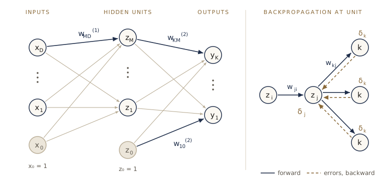
Two remarks on names. The network in the figure has two layers of adaptive weights, and we call it a two-layer network; you will also see it called a three-layer network (counting layers of units) or a single-hidden-layer network. And “multilayer perceptron” is a slightly misleading name: each unit is a smooth, differentiable function of its inputs, much more like a small logistic regression than like the step-function perceptron of module 04. That differentiability is what makes gradient-based training possible.
Here is the network in code. We store all parameters in one flat vector w, since optimizers, gradient checks, and Hessians all want a single vector, and unpack returns views of it as the matrices of the formula. W1 has shape (M, D), so row \(j\) holds the weights \(w^{(1)}_{ji}\) into hidden unit \(j\); one matrix product then computes the activations of all hidden units for all \(N\) inputs at once.
import numpy as np
from itertools import permutations, product
from math import factorial
from time import perf_counter
from scipy.special import expit, logsumexp

np.set_printoptions(precision=4, suppress=True)
rng = np.random.default_rng(5)
def n_weights(arch):
    """W = M(D + 1) + K(M + 1) for arch = (D, M, K)."""
    D, M, K = arch
    return M * (D + 1) + K * (M + 1)

def unpack(w, arch):
    """Views of the flat parameter vector w as (W1, b1, W2, b2)."""
    D, M, K = arch
    s1, s2 = M * D, M * (D + 1)
    W1 = w[:s1].reshape(M, D)                  # w_ji^(1)
    b1 = w[s1:s2]                              # w_j0^(1)
    W2 = w[s2:s2 + K * M].reshape(K, M)        # w_kj^(2)
    b2 = w[s2 + K * M:]                        # w_k0^(2)
    return W1, b1, W2, b2

def init_weights(arch, rng):
    """Random start: w_ji^(1) ~ N(0, 1/D), w_j0^(1) ~ N(0, 1), w_kj^(2) ~ N(0, 1/M),
    and output biases w_k0^(2) = 0."""
    D, M, K = arch
    return np.concatenate([rng.normal(0, 1 / np.sqrt(D), M * D), rng.normal(0, 1, M),
                           rng.normal(0, 1 / np.sqrt(M), K * M), np.zeros(K)])

def forward(w, X, arch):
    """Forward propagation for all N rows of X at once."""
    W1, b1, W2, b2 = unpack(w, arch)
    A1 = X @ W1.T + b1        # a_j = sum_i w_ji x_i + w_j0,   shape (N, M)
    Z = np.tanh(A1)           # z_j = h(a_j)
    A2 = Z @ W2.T + b2        # a_k = sum_j w_kj z_j + w_k0,   shape (N, K)
    return A1, Z, A2

def output(A2, kind):
    """Output activation: identity, logistic sigmoid, or softmax over each row."""
    if kind == "linear":
        return A2
    if kind == "sigmoid":
        return expit(A2)
    return np.exp(A2 - logsumexp(A2, axis=1, keepdims=True))

arch = (2, 3, 2)                    # D = 2 inputs, M = 3 hidden units, K = 2 outputs
w = init_weights(arch, rng)
X = rng.normal(size=(4, 2))
Y = output(forward(w, X, arch)[2], "sigmoid")

# the same outputs for the first input, from the formula written as explicit sums
W1, b1, W2, b2 = unpack(w, arch)
x = X[0]
y_sums = [expit(sum(W2[k, j] * np.tanh(sum(W1[j, i] * x[i] for i in range(2)) + b1[j])
                    for j in range(3)) + b2[k]) for k in range(2)]
print("W =", n_weights(arch), "parameters; w has", w.size, "entries")
print("sigmoid outputs for 4 inputs:\n", Y)
print("explicit sums, first input:", np.round(y_sums, 4))
W = 17 parameters; w has 17 entries
sigmoid outputs for 4 inputs:
 [[0.6847 0.3193]
 [0.6526 0.2776]
 [0.5075 0.3018]
 [0.2084 0.4514]]
explicit sums, first input: [0.6847 0.3193]
The vectorized forward pass and the literal double sum agree. With \(D = 2\), \(M = 3\), and \(K = 2\) the network has \(3 \cdot 3 + 2 \cdot 4 = 17\) parameters.
More general networks
Why a nonlinear \(h\)? If every hidden unit were linear, the whole network would be a composition of linear maps, which is again a linear map, and nothing would be gained over module 03. (With fewer hidden units than inputs and outputs, a linear network is a rank-limited linear map; module 12 shows that such networks relate to principal component analysis.)
The two-layer architecture is the most common, but the same construction extends in several directions. We can stack more layers, each a weighted sum followed by an elementwise nonlinearity. We can add skip-layer connections, for example weights that go straight from the inputs to the outputs. And we can leave out connections, as the convolutional networks later in this module do. In general, any directed graph of units without directed cycles defines a network: each unit computes
\[z_k = h\left( \sum_j w_{kj} z_j \right),\]where the sum runs over the units \(j\) that send a connection to \(k\) (with a bias included), and evaluating the units in an order in which every unit comes after all of its inputs gives the outputs. The requirement of no directed cycles is what makes the network feed-forward, so that its outputs are deterministic functions of its inputs.
Watch out. Network diagrams look like the graphical models of module 08, but they mean something different. The nodes of a network diagram are deterministic quantities computed from their inputs, not random variables, and the links are parameters, not conditional distributions. A probabilistic reading of a network comes only from the likelihood we attach to its outputs, which is the topic of the next section.
Universal approximation
How much can a two-layer network represent? A great deal. A classical family of results, proved in several forms around 1989, shows that a network with one hidden layer and linear outputs can approximate any continuous function on a compact (closed and bounded) region of input space to any desired accuracy, provided it has enough hidden units. The result holds for a wide range of activation functions, including \(\tanh\) and the logistic sigmoid, though not for polynomial ones. For this reason neural networks are called universal approximators.
The theorem says a good network exists; it does not say how to find its weights from a finite, noisy data set, or how many hidden units that takes. The rest of the module is about finding the weights. Once we can train a network, we will fit a network with only three hidden units to four quite different functions and look at how the hidden units share the work (the figure in the section on training below).
Weight-space symmetries
A network function does not determine its weight vector. Take a two-layer network with \(M\) tanh hidden units. Since \(\tanh\) is odd, \(\tanh(-a) = -\tanh(a)\), so flipping the signs of all weights and the bias into hidden unit \(j\) flips the sign of \(z_j\); flipping the signs of the weights out of unit \(j\) as well undoes the change at the outputs. Each of the \(M\) hidden units can be flipped independently, which gives \(2^M\) weight vectors with the same function. Independently of that, the hidden units can be relabeled: swapping all the weights in and out of unit \(j\) with those of unit \(j'\) changes \(\mathbf{w}\) but not the function, and there are \(M!\) orderings. So every weight vector belongs to a family of
\[2^M M!\]equivalent weight vectors. For a network with several hidden layers, the factors for the layers multiply. Apart from accidental coincidences for special weight values, these are all the symmetries, and similar ones exist for many other activation functions.
Let’s check this for \(M = 4\), where the count is \(2^4 \cdot 4! = 384\).
def transform(w, arch, signs, perm):
    """Flip the sign of hidden unit j where signs[j] = -1, then reorder units by perm."""
    W1, b1, W2, b2 = unpack(w, arch)
    s = np.asarray(signs, dtype=float)
    return np.concatenate([(s[:, None] * W1)[perm].ravel(), (s * b1)[perm],
                           (W2 * s)[:, perm].ravel(), b2])

arch = (2, 4, 1)
w = init_weights(arch, rng)
X = rng.normal(size=(5, 2))
y0 = forward(w, X, arch)[2]

flipped = transform(w, arch, [1, -1, 1, 1], [0, 1, 2, 3])
print(f"flip the second hidden unit only: weights change by up to"
      f" {np.abs(flipped - w).max():.3f}, outputs by"
      f" {np.abs(forward(flipped, X, arch)[2] - y0).max():.1e}")

variants = [transform(w, arch, s, list(p))
            for s in product([1, -1], repeat=4) for p in permutations(range(4))]
largest = max(np.abs(forward(v, X, arch)[2] - y0).max() for v in variants)
distinct = len({tuple(np.round(v, 10)) for v in variants})
print(len(variants), "transformations give", distinct, "distinct weight vectors;",
      "2^M M! =", 2 ** 4 * factorial(4))
print(f"largest change in any output: {largest:.1e}")
flip the second hidden unit only: weights change by up to 2.324, outputs by 0.0e+00
384 transformations give 384 distinct weight vectors; 2^M M! = 384
largest change in any output: 1.1e-16
All 384 weight vectors are different, and all compute the same outputs up to round-off. For most purposes this redundancy is harmless: an optimizer finds one member of the family and any member will do. It matters when we count or compare modes of a posterior distribution, which we will do in the Bayesian section at the end.
Network training
Error functions from likelihoods
The simplest way to fit a network is to copy polynomial curve fitting from module 01 and minimize a sum of squares. A better route, which also tells us which output activation to use, is to give the outputs a probabilistic meaning and minimize a negative log likelihood. The three standard cases follow.
Regression. Take one real target \(t\) and assume it is Gaussian around the network output, with noise precision \(\beta\):
\[p(t \mid \mathbf{x}, \mathbf{w}, \beta) = \mathcal{N}\left(t \mid y(\mathbf{x}, \mathbf{w}), \beta^{-1}\right).\]A network with identity outputs can approximate any continuous mean function, so the identity is the natural output activation here. For \(N\) independent observations, the negative log likelihood is
\[\frac{\beta}{2} \sum_{n=1}^{N} \{ y(\mathbf{x}_n, \mathbf{w}) - t_n \}^2 - \frac{N}{2} \ln \beta + \frac{N}{2} \ln(2\pi).\]As a function of \(\mathbf{w}\), only the first term matters, so maximizing the likelihood means minimizing the sum-of-squares error
\[E(\mathbf{w}) = \frac{1}{2} \sum_{n=1}^{N} \{ y(\mathbf{x}_n, \mathbf{w}) - t_n \}^2 .\]Call its minimizer \(\mathbf{w}_{\mathrm{ML}}\). Because \(y\) depends nonlinearly on \(\mathbf{w}\), this error is not convex, and in practice we find a local minimum rather than a guaranteed global one. Given \(\mathbf{w}_{\mathrm{ML}}\), setting the derivative with respect to \(\beta\) to zero gives the noise estimate
\[\frac{1}{\beta_{\mathrm{ML}}} = \frac{1}{N} \sum_{n=1}^{N} \{ y(\mathbf{x}_n, \mathbf{w}_{\mathrm{ML}}) - t_n \}^2 .\]With \(K\) targets that are independent given \(\mathbf{x}\) and share the precision \(\beta\), the error becomes \(\tfrac12 \sum_n \lVert \mathbf{y}(\mathbf{x}_n, \mathbf{w}) - \mathbf{t}_n \rVert^2\) and the estimate of \(1/\beta\) divides by \(NK\) instead of \(N\). (Correlated targets with a full noise covariance also work, at the cost of a harder optimization; see Bishop’s exercise 5.3.)
For one data point, \(E_n = \tfrac12 \sum_k (y_k - t_k)^2\) with \(y_k = a_k\), so the derivative with respect to an output activation is
\[\frac{\partial E_n}{\partial a_k} = y_k - t_k .\]This little formula is the starting point of backpropagation, and it will reappear in the other two cases.
Binary classification. Let \(t = 1\) stand for class \(\mathcal{C}_1\) and \(t = 0\) for \(\mathcal{C}_2\). A single output with a logistic sigmoid, \(y = \sigma(a) = 1/(1 + e^{-a})\), lies between 0 and 1, and we read it as \(p(\mathcal{C}_1 \mid \mathbf{x})\). The target is then Bernoulli, \(p(t \mid \mathbf{x}, \mathbf{w}) = y^t (1 - y)^{1 - t}\), and the negative log likelihood is the cross-entropy error
\[E(\mathbf{w}) = -\sum_{n=1}^{N} \{ t_n \ln y_n + (1 - t_n) \ln(1 - y_n) \}, \qquad y_n = y(\mathbf{x}_n, \mathbf{w}).\]There is no \(\beta\) here because the labels are assumed correct (Bishop’s exercise 5.4 extends the model to labels that are sometimes flipped). To differentiate, use \(\sigma'(a) = \sigma(a)\{1 - \sigma(a)\}\):
\[\frac{\partial E_n}{\partial a} = \left( -\frac{t}{y} + \frac{1 - t}{1 - y} \right) y (1 - y) = -t(1 - y) + (1 - t) y = y - t .\]For \(K\) separate yes/no decisions, such as tagging an image with any subset of \(K\) labels, use \(K\) sigmoid outputs and add their cross-entropies; the derivative is \(y_k - t_k\) for each. It is worth comparing this with fitting \(K\) separate logistic regressions as in module 04. In the network all \(K\) outputs share the first layer, which acts as a learned feature extractor; the shared features save computation and can help each task learn from the others.
Multiclass classification. For \(K\) mutually exclusive classes with one-hot targets \(t_k \in \{0, 1\}\), use a softmax output,
\[y_k(\mathbf{x}, \mathbf{w}) = \frac{\exp(a_k)}{\sum_{j} \exp(a_j)},\]read \(y_k\) as \(p(t_k = 1 \mid \mathbf{x})\), and minimize the multiclass cross-entropy
\[E(\mathbf{w}) = -\sum_{n=1}^{N} \sum_{k=1}^{K} t_{nk} \ln y_k(\mathbf{x}_n, \mathbf{w}).\]The softmax derivatives are \(\partial y_k / \partial a_j = y_k (I_{kj} - y_j)\), where \(I_{kj}\) is 1 if \(k = j\) and 0 otherwise. So, for one data point,
\[\frac{\partial E_n}{\partial a_j} = -\sum_{k} \frac{t_k}{y_k} y_k (I_{kj} - y_j) = -t_j + y_j \sum_k t_k = y_j - t_j ,\]using \(\sum_k t_k = 1\). Adding the same constant to every \(a_k\) leaves the softmax unchanged, so the error is flat along some directions in weight space; a regularizer (later in this module) removes that degeneracy. For two classes, one sigmoid output and two softmax outputs are equivalent.
| Problem | Output activation | Error function | \(\partial E_n / \partial a_k\) |
|---|---|---|---|
| Regression | identity | sum of squares | \(y_k - t_k\) |
| \(K\) independent binary labels | logistic sigmoid per output | sum of binary cross-entropies | \(y_k - t_k\) |
| One of \(K\) classes | softmax | multiclass cross-entropy | \(y_k - t_k\) |
Result. When the output activation and the error function are paired as in the table (in the language of module 04, the output activation is the canonical link for the target distribution), the derivative of the error for one data point with respect to each output activation is \(\partial E_n / \partial a_k = y_k - t_k\): prediction minus target.
In code, each error function is computed from the output activations \(a_k\) rather than from the outputs \(y_k\). That keeps the logarithms stable: for the binary case, \(-t \ln \sigma(a) - (1 - t)\ln(1 - \sigma(a))\) simplifies to \(\ln(1 + e^{a}) - t a\), which np.logaddexp evaluates without overflow, and for the softmax, \(\ln y_k = a_k - \ln \sum_j e^{a_j}\) is a log-sum-exp. We check the “prediction minus target” rule numerically for all three pairs.
def error(A2, T, kind):
    """Negative log likelihood matched to the output activation, computed from A2."""
    if kind == "linear":                                    # sum of squares
        return 0.5 * np.sum((A2 - T) ** 2)
    if kind == "sigmoid":                                   # binary cross-entropy
        return np.sum(np.logaddexp(0, A2) - T * A2)
    return -np.sum(T * (A2 - logsumexp(A2, axis=1, keepdims=True)))   # multiclass

a = rng.normal(size=(1, 3))
cases = {"linear": rng.normal(size=(1, 3)), "sigmoid": np.array([[1.0, 0.0, 1.0]]),
         "softmax": np.array([[0.0, 1.0, 0.0]])}
eps = 1e-6
for kind, t in cases.items():
    numeric = [(error(a + eps * e, t, kind) - error(a - eps * e, t, kind)) / (2 * eps)
               for e in np.eye(3)]
    print(f"{kind:8s} y - t = {output(a, kind)[0] - t[0]}"
          f"   numerical dE/da = {np.array(numeric)}")
linear   y - t = [-0.9938  2.061  -0.8502]   numerical dE/da = [-0.9938  2.061  -0.8502]
sigmoid  y - t = [-0.5636  0.7235 -0.7652]   numerical dE/da = [-0.5636  0.7235 -0.7652]
softmax  y - t = [ 0.2094 -0.2924  0.083 ]   numerical dE/da = [ 0.2094 -0.2924  0.083 ]
The two columns agree to the printed precision in every row.
Parameter optimization
Picture the error \(E(\mathbf{w})\) as a surface over weight space. A small step \(\delta\mathbf{w}\) changes the error by \(\delta E \approx \delta\mathbf{w}^{\mathrm{T}} \nabla E(\mathbf{w})\), and the gradient \(\nabla E\) points in the direction in which the error increases fastest. At the smallest value of a smooth error the gradient must vanish,
\[\nabla E(\mathbf{w}) = \mathbf{0},\]since otherwise a small step along \(-\nabla E\) would lower the error further. Points where the gradient vanishes are stationary points; they can be minima, maxima, or saddle points.
The error of a network has many stationary points. By the weight-space symmetries, every minimum comes with \(2^M M! - 1\) equivalent copies. Beyond those, there are usually several inequivalent minima with different error values. The lowest is the global minimum; the others are local minima. In practice we rarely know whether we have found the global minimum, and we do not need to: it is usually enough to train from several random starting points and keep the solution that does best on validation data.
There is no hope of solving \(\nabla E = \mathbf{0}\) in closed form, so all training methods are iterative. They start from some \(\mathbf{w}^{(0)}\) and take steps
\[\mathbf{w}^{(\tau + 1)} = \mathbf{w}^{(\tau)} + \Delta \mathbf{w}^{(\tau)},\]where \(\tau\) counts the steps. Methods differ in how they choose \(\Delta\mathbf{w}^{(\tau)}\); most of them use the gradient at the current point. A local quadratic model of the error explains why.
Local quadratic approximation
Expand the error in a Taylor series around a point \(\widehat{\mathbf{w}}\) and stop after the quadratic term:
\[E(\mathbf{w}) \approx E(\widehat{\mathbf{w}}) + (\mathbf{w} - \widehat{\mathbf{w}})^{\mathrm{T}} \mathbf{b} + \frac{1}{2} (\mathbf{w} - \widehat{\mathbf{w}})^{\mathrm{T}} \mathbf{H} (\mathbf{w} - \widehat{\mathbf{w}}).\]Here \(\mathbf{b} = \nabla E\) evaluated at \(\widehat{\mathbf{w}}\), and \(\mathbf{H}\) is the Hessian matrix of second derivatives, \(H_{ij} = \partial^2 E / \partial w_i \partial w_j\) at \(\widehat{\mathbf{w}}\). Differentiating, the gradient near \(\widehat{\mathbf{w}}\) is approximately \(\nabla E \approx \mathbf{b} + \mathbf{H}(\mathbf{w} - \widehat{\mathbf{w}})\).
At a minimum \(\mathbf{w}^{\star}\) the linear term vanishes, and
\[E(\mathbf{w}) \approx E(\mathbf{w}^{\star}) + \frac{1}{2} (\mathbf{w} - \mathbf{w}^{\star})^{\mathrm{T}} \mathbf{H} (\mathbf{w} - \mathbf{w}^{\star}).\]The Hessian is symmetric, so it has orthonormal eigenvectors, \(\mathbf{H}\mathbf{u}_i = \lambda_i \mathbf{u}_i\) with \(\mathbf{u}_i^{\mathrm{T}} \mathbf{u}_j = I_{ij}\). Write the displacement in this basis, \(\mathbf{w} - \mathbf{w}^{\star} = \sum_i \alpha_i \mathbf{u}_i\). Then
\[E(\mathbf{w}) \approx E(\mathbf{w}^{\star}) + \frac{1}{2} \sum_i \lambda_i \alpha_i^2 .\]In these rotated coordinates the error is a sum of independent parabolas. If every \(\lambda_i > 0\), which is exactly the condition for \(\mathbf{H}\) to be positive definite (\(\mathbf{v}^{\mathrm{T}} \mathbf{H} \mathbf{v} > 0\) for every \(\mathbf{v} \neq \mathbf{0}\)), the error rises in every direction and \(\mathbf{w}^{\star}\) is a local minimum. The contours of constant error are then ellipses (ellipsoids in more dimensions) with axes along the eigenvectors, and the axis along \(\mathbf{u}_i\) has length proportional to \(\lambda_i^{-1/2}\): large curvature means a short axis. So a stationary point at which the Hessian is positive definite is a local minimum, the many-dimensional version of “the second derivative is positive”.
Why gradients help
The quadratic model is specified by \(\mathbf{b}\) and \(\mathbf{H}\), which together contain \(W + W(W+1)/2 = W(W+3)/2\) independent numbers. So we should expect to need on the order of \(W^2\) pieces of information before we can locate the minimum. If we can only evaluate the error, each evaluation gives one number and costs \(O(W)\) operations, so finding the minimum costs \(O(W^2) \times O(W) = O(W^3)\). A gradient evaluation gives \(W\) numbers at once. If it also costs only \(O(W)\), which backpropagation achieves, then \(O(W)\) gradient evaluations suffice and the total is \(O(W^2)\). For a network with a million weights, that factor of \(W\) is the difference between feasible and hopeless.
Gradient descent
The simplest use of the gradient is to step downhill:
\[\mathbf{w}^{(\tau + 1)} = \mathbf{w}^{(\tau)} - \eta \nabla E(\mathbf{w}^{(\tau)}),\]where \(\eta > 0\) is the learning rate. When \(E\) is summed over the whole training set, every step processes all the data; such methods are called batch methods, and this one is gradient descent (or steepest descent).
Gradient descent is a weak optimizer on its own. The quadratic model shows why. Along eigenvector \(\mathbf{u}_i\) one step multiplies the distance to the minimum by \(1 - \eta\lambda_i\). Stability needs \(\eta < 2/\lambda_{\max}\), and then the direction with the smallest curvature shrinks by only a factor of about \(1 - \lambda_{\min}/\lambda_{\max}\) per step. The number of steps grows in proportion to the condition number \(\lambda_{\max}/\lambda_{\min}\), which for networks is often huge. A common remedy is momentum, which adds a fraction \(\mu\) of the previous step to the current one,
\[\Delta\mathbf{w}^{(\tau)} = -\eta \nabla E(\mathbf{w}^{(\tau)}) + \mu \Delta\mathbf{w}^{(\tau - 1)},\]so that consistent components of the gradient accumulate while oscillating components cancel. Here are both methods on a two-dimensional quadratic \(E = \tfrac12 \mathbf{w}^{\mathrm{T}}\mathbf{H}\mathbf{w}\) with eigenvalues 1 and \(\kappa\), counting steps until \(E < 10^{-8}\).
def descend(H, w0, eta, mu=0.0, tol=1e-8, max_steps=100_000):
    """Gradient descent with momentum mu on E = w^T H w / 2; steps until E < tol."""
    w, step = w0.copy(), np.zeros_like(w0)
    for tau in range(max_steps):
        if 0.5 * w @ H @ w < tol:
            return tau
        step = -eta * (H @ w) + mu * step        # mu = 0: plain gradient descent
        w = w + step
    return max_steps

w0 = np.array([1.0, 1.0])
for kappa in [10, 100, 1000]:
    H = np.diag([1.0, kappa])                    # eigenvalues 1 and kappa
    eta = 1.0 / kappa                            # safely below the limit 2 / kappa
    print(f"condition number {kappa:4d}:  plain {descend(H, w0, eta):5d} steps,"
          f"  momentum 0.9 {descend(H, w0, eta, mu=0.9):4d} steps")
condition number   10:  plain    85 steps,  momentum 0.9  170 steps
condition number  100:  plain   882 steps,  momentum 0.9  176 steps
condition number 1000:  plain  8860 steps,  momentum 0.9  803 steps
Plain gradient descent needs about ten times more steps each time the condition number grows tenfold. Momentum is not free: on the easy problem it takes twice as many steps, because with \(\mu = 0.9\) the iterates overshoot and ring before they settle. But on the harder problems it needs about a fifth and then about a tenth as many steps as plain gradient descent. For batch training there are stronger methods still, such as conjugate gradients and quasi-Newton methods, which are much faster and more robust than plain gradient descent and, unlike it, never let the error go up from one iteration to the next. Bishop §5.2.4 gives references. Whatever the optimizer, it is wise to run it from several random starting points and compare the solutions on validation data.
For large data sets the most useful variant goes the other way. Error functions from independent data are sums over data points, \(E(\mathbf{w}) = \sum_n E_n(\mathbf{w})\), and stochastic gradient descent (also called on-line or sequential gradient descent) updates after each point,
\[\mathbf{w}^{(\tau + 1)} = \mathbf{w}^{(\tau)} - \eta \nabla E_n(\mathbf{w}^{(\tau)}),\]cycling through the data in order or picking points at random; in between lie mini-batches of a few dozen points. Two arguments favor it. First, real data are redundant. If we duplicated every data point, the batch gradient would cost twice as much to compute but would point in the same direction, while stochastic gradient descent would not notice any difference. Second, a stationary point of the total error is generally not a stationary point of the individual \(E_n\), so the noise in the updates can carry the weights out of a poor local minimum. We compare batch and mini-batch training on a real network after we can compute gradients.
Error backpropagation
We now need the gradient \(\nabla E(\mathbf{w})\) of a network’s error, and we want it in \(O(W)\) operations. Error backpropagation, or backprop, does this by passing information forward through the network and then errors backward.
The word “backpropagation” is used loosely in the literature, sometimes for the whole training procedure or even for the network architecture. It helps to separate two stages of each training step. In the first, we compute the gradient of the error in weight space; in the second, an optimizer uses them to change the weights. We use “backpropagation” only for the first stage. It works for any feed-forward architecture and any differentiable error, and it computes other derivatives too, such as the Jacobian and the Hessian. The second stage can be any gradient-based optimizer, from gradient descent to quasi-Newton methods.
Deriving backpropagation
Error functions from independent data are sums of one term per data point, \(E = \sum_n E_n\), so it suffices to compute \(\nabla E_n\) and add. To keep the notation light we drop the index \(n\) from the unit values.
Start with a warm-up: a linear model \(y_k = \sum_i w_{ki} x_i\) with \(E_n = \tfrac12 \sum_k (y_k - t_k)^2\). The derivative with respect to one weight is
\[\frac{\partial E_n}{\partial w_{ki}} = (y_k - t_k)\, x_i .\]It is a product of two local quantities: an “error” \(y_k - t_k\) at the output end of the connection and the value \(x_i\) at its input end. Backpropagation extends this pattern to any feed-forward network.
In a general feed-forward network, unit \(j\) computes a weighted sum of the values \(z_i\) of the units (or inputs) that feed it, and applies its activation function:
\[a_j = \sum_i w_{ji} z_i, \qquad z_j = h(a_j).\]Biases are included through a unit whose value is always 1. Suppose we have run forward propagation, so every \(a_j\) and \(z_j\) is known. The error depends on the weight \(w_{ji}\) only through the sum \(a_j\), so by the chain rule
\[\frac{\partial E_n}{\partial w_{ji}} = \frac{\partial E_n}{\partial a_j} \frac{\partial a_j}{\partial w_{ji}} .\]The second factor is \(\partial a_j / \partial w_{ji} = z_i\). For the first, introduce the notation
\[\delta_j \equiv \frac{\partial E_n}{\partial a_j},\]and call \(\delta_j\) the error of unit \(j\). Then
\[\frac{\partial E_n}{\partial w_{ji}} = \delta_j z_i ,\]the same “error times input” pattern as the linear model (with \(z_i = 1\) for a bias). So we only need the \(\delta\) of every hidden and output unit.
For the output units we already have them: with the matched pairs of the previous section, \(\delta_k = y_k - t_k\). For a hidden unit \(j\), the error \(E_n\) depends on \(a_j\) only through the activations \(a_k\) of the units \(k\) that \(j\) sends connections to. The chain rule gives
\[\delta_j = \frac{\partial E_n}{\partial a_j} = \sum_k \frac{\partial E_n}{\partial a_k} \frac{\partial a_k}{\partial a_j} .\]Since \(a_k = \sum_j w_{kj} h(a_j)\), we have \(\partial a_k / \partial a_j = w_{kj} h'(a_j)\), and so
\[\delta_j = h'(a_j) \sum_k w_{kj} \delta_k .\]This is the backpropagation formula. The error of a hidden unit is a weighted sum of the errors of the units it feeds, times the slope of its own activation function. Compare it with forward propagation, \(a_j = \sum_i w_{ji} z_i\): going forward we sum over the second index of the weights, going backward over the first. Starting from the output errors and applying the formula unit by unit, in the reverse of the forward order, gives the \(\delta\) of every hidden unit in any feed-forward network.
Result. Error backpropagation, for one data point:
- Forward-propagate the input \(\mathbf{x}_n\) to get every \(a_j\) and \(z_j\).
- Compute the output errors \(\delta_k = y_k - t_k\).
- Propagate backward: \(\delta_j = h'(a_j) \sum_k w_{kj} \delta_k\) for every hidden unit.
- Read off the derivatives \(\partial E_n / \partial w_{ji} = \delta_j z_i\).
For a batch error, repeat for every data point and add: \(\partial E / \partial w_{ji} = \sum_n \partial E_n / \partial w_{ji}\).
If different units use different activation functions, the derivation is the same; each unit simply uses its own \(h'\).
A two-layer network in NumPy
For our two-layer network with \(\tanh\) hidden units, the derivative has a convenient form, \(h'(a) = 1 - \tanh^2(a) = 1 - z^2\), so the backward pass needs only the hidden values we already stored. For one data point:
\[\delta_k = y_k - t_k, \qquad \delta_j = (1 - z_j^2) \sum_{k=1}^{K} w^{(2)}_{kj} \delta_k, \qquad \frac{\partial E_n}{\partial w^{(1)}_{ji}} = \delta_j x_i, \qquad \frac{\partial E_n}{\partial w^{(2)}_{kj}} = \delta_k z_j .\]For all \(N\) points at once, stack the errors into matrices: \(\boldsymbol{\Delta}_2 = \mathbf{Y} - \mathbf{T}\) of shape \(N \times K\) and \(\boldsymbol{\Delta}_1 = (1 - \mathbf{Z}^2) \odot (\boldsymbol{\Delta}_2 \mathbf{W}_2)\) of shape \(N \times M\), where \(\odot\) is the elementwise product. Summing the per-point derivatives over \(n\) is then a matrix product: \(\boldsymbol{\Delta}_2^{\mathrm{T}} \mathbf{Z}\) for the second-layer weights and \(\boldsymbol{\Delta}_1^{\mathrm{T}} \mathbf{X}\) for the first; the bias gradients are column sums. We split the code into backward, which takes any output errors, and backprop, which supplies \(\delta_k = y_k - t_k\); the mixture density network later supplies its own output errors to the same backward.
def backward(w, X, Z, d2, arch):
    """Backpropagate output errors d2 = dE/da_k, shape (N, K).
    Returns the gradient, summed over the N data points."""
    W1, b1, W2, b2 = unpack(w, arch)
    d1 = (1 - Z ** 2) * (d2 @ W2)     # delta_j = h'(a_j) sum_k w_kj delta_k, h' = 1 - z^2
    return np.concatenate([(d1.T @ X).ravel(), d1.sum(0),     # dE/dw_ji = delta_j x_i
                           (d2.T @ Z).ravel(), d2.sum(0)])    # dE/dw_kj = delta_k z_j

def backprop(w, X, T, arch, kind="linear"):
    """Error E(w) and its gradient, with matched output activation and error."""
    A1, Z, A2 = forward(w, X, arch)
    d2 = output(A2, kind) - T               # delta_k = y_k - t_k
    return error(A2, T, kind), backward(w, X, Z, d2, arch)
Now the essential test. Any bug in a gradient, such as a missing transpose or a wrong index, still leaves an optimizer running happily and converging to something, so we compare with central differences,
\[\frac{\partial E}{\partial w_i} \approx \frac{E(\mathbf{w} + \epsilon \mathbf{e}_i) - E(\mathbf{w} - \epsilon \mathbf{e}_i)}{2\epsilon},\]where \(\mathbf{e}_i\) is the \(i\)th unit vector. We report the largest relative difference, \(\lvert g - \tilde{g} \rvert / (\lvert g \rvert + \lvert \tilde{g} \rvert)\), over all components.
def numerical_gradient(f, w, eps=1e-6):
    """Central differences, one weight at a time: 2W evaluations of f."""
    g = np.zeros_like(w)
    for i in range(w.size):
        e = np.zeros_like(w)
        e[i] = eps
        g[i] = (f(w + e) - f(w - e)) / (2 * eps)
    return g

def max_rel_error(a, b):
    """Largest componentwise relative difference between two arrays."""
    return np.max(np.abs(a - b) / np.maximum(np.abs(a) + np.abs(b), 1e-8))

N, D, M, K = 20, 3, 5, 4
X = rng.normal(size=(N, D))
cases = {"linear": rng.normal(size=(N, K)),
         "sigmoid": rng.integers(0, 2, (N, K)).astype(float),
         "softmax": np.eye(K)[rng.integers(0, K, N)]}
arch = (D, M, K)
w = init_weights(arch, rng)
for kind, T in cases.items():
    E, g = backprop(w, X, T, arch, kind)
    g_num = numerical_gradient(lambda v: backprop(v, X, T, arch, kind)[0], w)
    print(f"{kind:8s} E = {E:8.4f}   W = {w.size}"
          f"   max relative error {max_rel_error(g, g_num):.1e}")
linear   E =  56.2401   W = 44   max relative error 2.4e-08
sigmoid  E =  52.9759   W = 44   max relative error 4.7e-08
softmax  E =  32.5204   W = 44   max relative error 7.6e-08
Relative errors around \(10^{-7}\) or below mean the two agree to the accuracy that finite differences can deliver. A real bug gives relative errors of order 1 in the affected components.
Efficiency of backpropagation
Count operations as a function of the number of weights \(W\). Forward propagation costs \(O(W)\): except in very sparse networks, the weighted sums dominate, and each weight contributes one multiplication and one addition. The backward pass visits each weight once more, and step 4 visits it a third time. So backpropagation computes all \(W\) derivatives in \(O(W)\) operations, a small constant times the cost of evaluating the network.
Finite differences need at least one extra evaluation per weight, and each evaluation costs \(O(W)\), so the whole gradient costs \(O(W^2)\). There is also a question of accuracy. A Taylor expansion shows that the one-sided difference \(\{E(w_i + \epsilon) - E(w_i)\}/\epsilon\) has error \(O(\epsilon)\). In the central difference the \(O(\epsilon)\) terms cancel, leaving \(O(\epsilon^2)\), at twice the cost. Neither can be pushed arbitrarily far by shrinking \(\epsilon\), because round-off in the subtraction grows like \(1/\epsilon\). The next cell shows both effects on one weight.
f = lambda v: backprop(v, X, cases["linear"], arch)[0]
g = backprop(w, X, cases["linear"], arch)[1]
i = 7
for eps in [1e-1, 1e-3, 1e-5, 1e-7, 1e-9]:
    e = np.zeros_like(w)
    e[i] = eps
    one_sided = (f(w + e) - f(w)) / eps
    central = (f(w + e) - f(w - e)) / (2 * eps)
    print(f"eps = {eps:.0e}   one-sided error {abs(one_sided - g[i]):.1e}"
          f"   central error {abs(central - g[i]):.1e}")
eps = 1e-01   one-sided error 4.4e-02   central error 6.0e-03
eps = 1e-03   one-sided error 3.7e-04   central error 6.0e-07
eps = 1e-05   one-sided error 3.7e-06   central error 2.4e-10
eps = 1e-07   one-sided error 1.4e-07   central error 3.7e-08
eps = 1e-09   one-sided error 6.1e-06   central error 2.6e-06
As \(\epsilon\) shrinks by a factor of 100, the one-sided error falls by about 100 and the central error by about \(10^4\), until round-off takes over and both get worse again. That is why central differences with \(\epsilon\) around \(10^{-5}\) to \(10^{-6}\) are the standard check. Now the cost, for networks of growing size (your times will differ):
def best_time(f, repeats):
    """Shortest of several wall-clock timings of f(), in seconds."""
    times = []
    for _ in range(repeats):
        t0 = perf_counter()
        f()
        times.append(perf_counter() - t0)
    return min(times)

rng_t = np.random.default_rng(0)
for M in [5, 20, 80]:
    arch_t = (10, M, 1)
    X_t, T_t = rng_t.normal(size=(100, 10)), rng_t.normal(size=(100, 1))
    w_t = init_weights(arch_t, rng_t)
    t_bp = best_time(lambda: backprop(w_t, X_t, T_t, arch_t), 50)
    E_t = lambda v: backprop(v, X_t, T_t, arch_t)[0]
    t_fd = best_time(lambda: numerical_gradient(E_t, w_t), 1)
    print(f"W = {w_t.size:4d}   backprop {1e3 * t_bp:5.2f} ms"
          f"   finite differences {1e3 * t_fd:6.1f} ms   ratio {t_fd / t_bp:6.0f}")
W =   61   backprop  0.03 ms   finite differences    3.7 ms   ratio    145
W =  241   backprop  0.03 ms   finite differences   20.4 ms   ratio    599
W =  961   backprop  0.07 ms   finite differences  170.7 ms   ratio   2310
At these small sizes the backpropagation time hardly changes, because fixed overheads of the NumPy calls dominate it, while the finite-difference time grows faster than \(W\). The ratio runs from the hundreds into the thousands and keeps growing with \(W\), as the operation counts predict: every finite-difference gradient repeats the whole forward pass \(2W\) times.
In practice. Always compute gradients by backpropagation, and always check your implementation against central differences on a small network and a few data points before trusting it. Automatic differentiation libraries such as the ones behind PyTorch and JAX implement exactly this backward pass for arbitrary computations, but the check is still worth doing whenever you write a gradient by hand, including custom layers and custom losses.
Training a network
With gradients in hand we can train. We use Adam, a variant of stochastic gradient descent introduced by Kingma and Ba that is the default in much of modern practice. It keeps running averages of the gradient, \(\mathbf{m}\), and of its elementwise square, \(\mathbf{v}\), and steps by \(\eta\, \widehat{\mathbf{m}} / (\sqrt{\widehat{\mathbf{v}}} + \epsilon)\) elementwise, where the hats denote the averages corrected for their start at zero. The first average acts like momentum; dividing by the root of the second gives each weight its own step size, which helps with the badly conditioned error surfaces we just saw. It is not guaranteed to decrease the error at every step, but it is robust and needs little tuning.
def adam(fg, w, steps, lr=0.01, beta1=0.9, beta2=0.999, eps=1e-8, callback=None):
    """Minimize with Adam. fg(w) returns (E, gradient); callback(tau, w) runs after
    every step."""
    w = w.copy()
    m, v = np.zeros_like(w), np.zeros_like(w)
    for tau in range(1, steps + 1):
        E, g = fg(w)
        m = beta1 * m + (1 - beta1) * g              # running mean of the gradient
        v = beta2 * v + (1 - beta2) * g ** 2         # running mean of its square
        w -= lr * (m / (1 - beta1 ** tau)) / (np.sqrt(v / (1 - beta2 ** tau)) + eps)
        if callback is not None:
            callback(tau, w)
    return w
Our first training run returns to universal approximation. We draw 50 inputs uniformly from \((-1, 1)\), evaluate four functions on them (a parabola, a sine, the absolute value, and a step), and fit each with a network of only three tanh hidden units and a linear output.
funcs = {"x^2": lambda x: x ** 2, "sin(pi x)": lambda x: np.sin(np.pi * x),
         "abs(x)": np.abs, "step": lambda x: (x > 0).astype(float)}
rng_ua = np.random.default_rng(1)
x = np.sort(rng_ua.uniform(-1, 1, 50))
X = x[:, None]
arch = (1, 3, 1)
fits = {}
for name, f in funcs.items():
    T = f(x)[:, None]
    fits[name] = adam(lambda v: backprop(v, X, T, arch), init_weights(arch, rng_ua),
                      3000, lr=0.05)
    E = backprop(fits[name], X, T, arch)[0]
    print(f"{name:10s} RMS error {np.sqrt(2 * E / len(x)):.4f}")
x^2        RMS error 0.0039
sin(pi x)  RMS error 0.0016
abs(x)     RMS error 0.0264
step       RMS error 0.0249
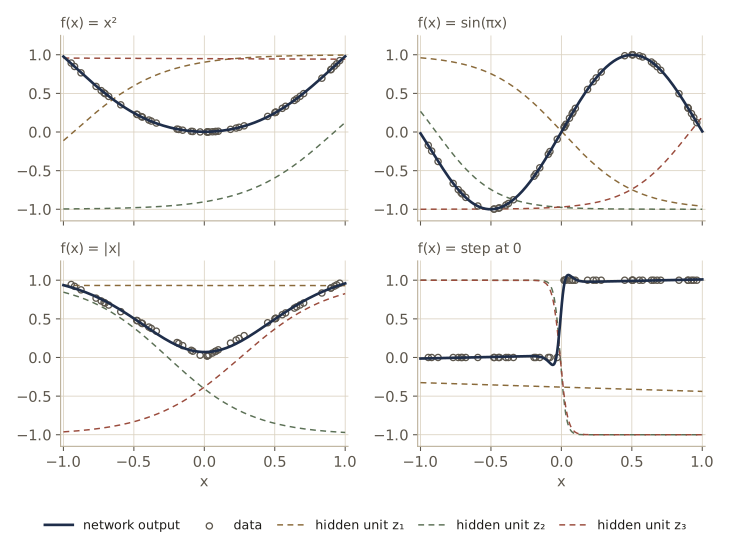
The parabola and the sine are fitted to within a few thousandths. The absolute value, with its kink, and the step, with its jump, are harder: a sum of three tanh curves is smooth, so it rounds off the kink and replaces the jump by a steep ramp, and most of the remaining error sits near \(x = 0\). The dashed curves in the figure show the division of labor: each hidden unit contributes one sigmoidal “bend”, placed and scaled by its weights.
Now the comparison promised in the section on gradient descent: batch gradient descent against mini-batch stochastic gradient descent on 2,000 noisy points from \(\sin(2\pi x)\), using a network with 10 hidden units and the same number of passes through the data (epochs) for both. Both use the mean error over the points they see, so that one learning rate works for any batch size.
def sin_data(N, rng, noise=0.3):
    """N inputs uniform on (0, 1) with targets sin(2 pi x) plus Gaussian noise."""
    x = rng.uniform(0, 1, N)
    return x[:, None], (np.sin(2 * np.pi * x) + rng.normal(0, noise, N))[:, None]

def rms(w, X, T, arch):
    """Root-mean-square error of a network with one linear output."""
    return np.sqrt(2 * backprop(w, X, T, arch)[0] / len(X))

rng_sgd = np.random.default_rng(2)
X, T = sin_data(2000, rng_sgd, noise=0.2)
arch = (1, 10, 1)
w_batch = w_sgd = init_weights(arch, rng_sgd)
eta = 0.2
print(f"at the start:     RMS {rms(w_batch, X, T, arch):.3f}")
for epoch in range(1, 51):
    w_batch = w_batch - eta * backprop(w_batch, X, T, arch)[1] / len(X)   # 1 step
    for idx in np.split(rng_sgd.permutation(len(X)), 100):                 # 100 steps
        w_sgd = w_sgd - eta * backprop(w_sgd, X[idx], T[idx], arch)[1] / len(idx)
    if epoch in (1, 5, 20, 50):
        print(f"after {epoch:2d} epochs:  batch RMS {rms(w_batch, X, T, arch):.3f}"
              f"   mini-batch (20 points) RMS {rms(w_sgd, X, T, arch):.3f}")
at the start:     RMS 1.313
after  1 epochs:  batch RMS 0.850   mini-batch (20 points) RMS 0.496
after  5 epochs:  batch RMS 0.749   mini-batch (20 points) RMS 0.470
after 20 epochs:  batch RMS 0.570   mini-batch (20 points) RMS 0.221
after 50 epochs:  batch RMS 0.482   mini-batch (20 points) RMS 0.210
Both runs use the learning rate 0.2 (much larger rates make the batch run unstable). They touch every data point equally often and cost about the same, but the mini-batch run makes 100 updates per epoch instead of one. The noise level here is 0.2, so an RMS error near 0.2 means the fit is essentially complete. Mini-batch training is there after 20 epochs; batch gradient descent is still at 0.48 after 50.
The Jacobian matrix
Backpropagation computes other derivatives too. The Jacobian matrix of a network holds the derivatives of its outputs with respect to its inputs,
\[J_{ki} = \frac{\partial y_k}{\partial x_i},\]each taken with the other inputs held fixed. Jacobians matter when a network is one module of a larger differentiable system. If an error \(E\) depends on a parameter \(w\) of an earlier module through that module’s output \(\mathbf{z}\), which feeds the network, then
\[\frac{\partial E}{\partial w} = \sum_{k, j} \frac{\partial E}{\partial y_k} \frac{\partial y_k}{\partial z_j} \frac{\partial z_j}{\partial w},\]and the network’s Jacobian is the middle factor. The Jacobian also measures sensitivity: small errors \(\Delta x_i\) in the inputs cause errors \(\Delta y_k \approx \sum_i J_{ki} \Delta x_i\) in the outputs. Because the network is nonlinear, the Jacobian depends on the input, so it must be recomputed at each \(\mathbf{x}\), and the linear estimate holds only for small perturbations.
To derive the backward pass, write \(y_k\) as a function of the first-layer activations, which depend on \(x_i\) through \(a_j = \sum_i w_{ji} x_i\):
\[J_{ki} = \sum_j \frac{\partial y_k}{\partial a_j} \frac{\partial a_j}{\partial x_i} = \sum_j w_{ji} \frac{\partial y_k}{\partial a_j} .\]The derivatives \(\partial y_k / \partial a_j\) obey a recursion of the same shape as the one for \(\delta_j\), summing over the units \(l\) that unit \(j\) feeds:
\[\frac{\partial y_k}{\partial a_j} = \sum_l \frac{\partial y_k}{\partial a_l} \frac{\partial a_l}{\partial a_j} = h'(a_j) \sum_l w_{lj} \frac{\partial y_k}{\partial a_l} .\]It starts at the output units, where \(\partial y_k / \partial a_l\) comes from the output activation: \(I_{kl}\, \sigma'(a_l)\) for sigmoid outputs and \(y_k (I_{kl} - y_l)\) for a softmax. Each row \(k\) of the Jacobian is one backward pass; in matrix form we do all rows at once.
def jacobian(w, x, arch, kind="softmax"):
    """J[k, i] = dy_k / dx_i at a single input x, by backpropagation."""
    W1, b1, W2, b2 = unpack(w, arch)
    A1, Z, A2 = forward(w, x[None, :], arch)
    y = output(A2, kind)[0]
    if kind == "softmax":
        dy_da2 = np.diag(y) - np.outer(y, y)       # dy_k/da_l = y_k (I_kl - y_l)
    elif kind == "sigmoid":
        dy_da2 = np.diag(y * (1 - y))              # dy_k/da_l = I_kl sigma'(a_l)
    else:
        dy_da2 = np.eye(len(y))
    dy_da1 = (dy_da2 @ W2) * (1 - Z[0] ** 2)   # dy_k/da_j = h'(a_j) sum_l w_lj dy_k/da_l
    return dy_da1 @ W1                             # J_ki = sum_j w_ji dy_k/da_j

arch = (3, 5, 4)
w = init_weights(arch, rng)
x0 = rng.normal(size=3)
y_of = lambda x: output(forward(w, x[None, :], arch)[2], "softmax")[0]
J = jacobian(w, x0, arch)
eps = 1e-6
J_num = np.column_stack([(y_of(x0 + eps * e) - y_of(x0 - eps * e)) / (2 * eps)
                         for e in np.eye(3)])
print("Jacobian (4 outputs x 3 inputs):\n", J)
print(f"max relative error vs central differences: {max_rel_error(J, J_num):.1e}")
print("column sums:", J.sum(axis=0))
dx = 1e-3 * rng.normal(size=3)
dy = y_of(x0 + dx) - y_of(x0)
print(f"actual change {np.abs(dy).max():.3e},"
      f" error of the linear estimate J dx {np.abs(dy - J @ dx).max():.1e}")
Jacobian (4 outputs x 3 inputs):
 [[-0.0441 -0.0534 -0.0389]
 [ 0.0519 -0.0271  0.0184]
 [ 0.052   0.1314  0.0619]
 [-0.0599 -0.051  -0.0414]]
max relative error vs central differences: 8.2e-10
column sums: [0. 0. 0.]
actual change 1.622e-04, error of the linear estimate J dx 2.3e-08
The backpropagated Jacobian matches central differences, which need \(2D\) forward passes. Each column sums to zero, as it must: the softmax outputs always add up to 1, so no change of input can change their total. And for a small input perturbation, \(\mathbf{J}\,\Delta\mathbf{x}\) predicts the change of the outputs with an error that is several orders of magnitude smaller than the change itself.
The Hessian matrix
Backpropagation can also give second derivatives. Collect all weights and biases into \(\mathbf{w} = (w_1, \dots, w_W)\); the Hessian \(\mathbf{H}\) has elements \(H_{ij} = \partial^2 E / \partial w_i \partial w_j\). It appears throughout neural computing:
- Second-order optimization methods (Newton, quasi-Newton, Levenberg–Marquardt) use the curvature it describes.
- After a small change to the training data, a network can be retrained quickly from the Hessian at the old solution.
- Pruning methods use the inverse Hessian to find the weights whose removal changes the error least.
- The Laplace approximation of a Bayesian network needs it: its inverse gives the predictive error bars, its eigenvalues drive the hyperparameters, and its determinant enters the evidence (see the last section).
The Hessian has \(W^2\) elements, so no method can compute it in fewer than \(O(W^2)\) operations per data point; the good methods achieve that. The rest of this section surveys approximations and exact methods. To have a reference to compare against, we first compute the Hessian by central differences of the backpropagated gradient: perturb one weight at a time and difference the two gradients, which fills in one column of \(\mathbf{H}\) per weight. The subsection on finite differences below explains why this costs \(O(W^2)\).
We use a small regression network: 20 noisy points from \(\sin(2\pi x)\), four hidden units, trained with Adam.
def hessian_fd(grad, w, eps=1e-5):
    """Hessian by central differences of the gradient: column i from 2 gradients."""
    W = w.size
    H = np.zeros((W, W))
    for i in range(W):
        e = np.zeros(W)
        e[i] = eps
        H[:, i] = (grad(w + e) - grad(w - e)) / (2 * eps)
    return 0.5 * (H + H.T)                  # symmetrize away round-off

rng_h = np.random.default_rng(3)
X, T = sin_data(20, rng_h, noise=0.2)
arch = (1, 4, 1)
w_init = init_weights(arch, rng_h)
w_fit = adam(lambda v: backprop(v, X, T, arch), w_init, 4000, lr=0.02)
grad = lambda v: backprop(v, X, T, arch)[1]
H = hessian_fd(grad, w_fit)
lam = np.linalg.eigvalsh(H)
print(f"W = {w_fit.size}   RMS error {rms(w_fit, X, T, arch):.3f}"
      f"   gradient norm {np.linalg.norm(grad(w_fit)):.1e}")
print(f"Hessian eigenvalues from {lam.min():.2e} to {lam.max():.2e}")
W = 13   RMS error 0.190   gradient norm 4.0e-03
Hessian eigenvalues from -7.43e-04 to 1.43e+02
The largest eigenvalue is about 140, and the smallest is essentially zero; it even comes out slightly negative, because Adam has stopped near a minimum but not exactly at it, and along a nearly flat direction the sign of the curvature is decided by small effects. Such a spread is typical: a few directions in weight space are stiff and many are nearly flat, which is the badly conditioned situation in which plain gradient descent struggles.
Diagonal approximation
Some uses need the inverse Hessian, and inverting a diagonal matrix is trivial, so one cheap option keeps only the diagonal. For one data point, since \(a_j\) is linear in the weight \(w_{ji}\),
\[\frac{\partial^2 E_n}{\partial w_{ji}^2} = \frac{\partial^2 E_n}{\partial a_j^2} z_i^2 .\]Differentiating the backpropagation formula once more gives a backward recursion for the second derivatives with respect to activations:
\[\frac{\partial^2 E_n}{\partial a_j^2} = h'(a_j)^2 \sum_k \sum_{k'} w_{kj} w_{k'j} \frac{\partial^2 E_n}{\partial a_k \partial a_{k'}} + h''(a_j) \sum_k w_{kj} \frac{\partial E_n}{\partial a_k} .\]The approximation proposed by Becker and Le Cun drops the terms with \(k \neq k'\), leaving a recursion that needs only diagonal quantities and costs \(O(W)\). Its weakness is not the recursion but the premise: the Hessians of real networks are usually far from diagonal.
Our example has a single linear output with sum-of-squares error, so \(\partial^2 E_n / \partial a_k^2 = 1\) and there are no pairs \(k \neq k'\) to drop: the recursion gives the diagonal exactly. That makes it a clean test, and it lets us measure how much of the Hessian lies off the diagonal. For tanh, \(h''(a) = -2z(1 - z^2)\).
def hessian_diagonal(w, X, T, arch):
    """Diagonal of the sum-of-squares Hessian for a network with one linear output."""
    W1, b1, W2, b2 = unpack(w, arch)
    A1, Z, A2 = forward(w, X, arch)
    delta = A2 - T                                        # dE_n/da_k, shape (N, 1)
    hp, hpp = 1 - Z ** 2, -2 * Z * (1 - Z ** 2)           # h'(a_j), h''(a_j)
    d2E_da2 = hp ** 2 * W2[0] ** 2 + hpp * W2[0] * delta   # d2E_n/da_j^2
    return np.concatenate([
        (d2E_da2[:, :, None] * X[:, None, :] ** 2).sum(0).ravel(),   # weights: z_i = x_i
        d2E_da2.sum(0),                                              # biases: z_i = 1
        (Z ** 2).sum(0), [len(X)]])                                  # second layer: z_j^2

H_diag = hessian_diagonal(w_fit, X, T, arch)
off = H - np.diag(np.diag(H))
print(f"diagonal recursion vs reference: max relative error"
      f" {max_rel_error(H_diag, np.diag(H)):.1e}")
print(f"share of the Hessian (Frobenius norm) off the diagonal:"
      f" {np.linalg.norm(off) / np.linalg.norm(H):.2f}")
diagonal recursion vs reference: max relative error 1.7e-10
share of the Hessian (Frobenius norm) off the diagonal: 0.89
The recursion reproduces the diagonal, but the off-diagonal part is not small: it accounts for 89 percent of the matrix in the Frobenius norm, all of which the diagonal approximation throws away. Treat diagonal approximations as a computational convenience, not as a faithful picture of the curvature.
Outer-product approximation
For regression with one output and \(E = \tfrac12 \sum_n (y_n - t_n)^2\), differentiate twice:
\[\mathbf{H} = \nabla\nabla E = \sum_{n=1}^{N} \nabla y_n \nabla y_n^{\mathrm{T}} + \sum_{n=1}^{N} (y_n - t_n) \nabla\nabla y_n .\]The second sum is multiplied by the residuals. If the network fits the data well, the residuals are small and the term is small. There is also a statistical argument: the function that minimizes a sum-of-squares error is the conditional mean of the targets (module 01), so at a good fit the residuals \(y_n - t_n\) behave like zero-mean noise, and if they are uncorrelated with the second derivatives \(\nabla\nabla y_n\), the sum averages toward zero. Dropping it gives the outer-product or Levenberg–Marquardt approximation
\[\mathbf{H} \approx \sum_{n=1}^{N} \mathbf{b}_n \mathbf{b}_n^{\mathrm{T}}, \qquad \mathbf{b}_n = \nabla y_n = \nabla a_n ,\]where the last equality holds because the output activation is the identity. Each \(\mathbf{b}_n\) is one backward pass with the output error set to 1, costing \(O(W)\), and the outer products cost \(O(W^2)\). The approximation is always positive semidefinite, which the exact Hessian need not be. For a sigmoid output with cross-entropy error, the same reasoning gives \(\mathbf{H} \approx \sum_n y_n(1 - y_n) \mathbf{b}_n \mathbf{b}_n^{\mathrm{T}}\) (Bishop’s exercise 5.19), and softmax outputs have an analogous form.
We compare it with the reference Hessian at the trained weights and at the random starting weights.
def output_grads(w, X, arch):
    """Rows b_n = gradient of the single output activation a(x_n, w) with respect
    to w; shape (N, W)."""
    W1, b1, W2, b2 = unpack(w, arch)
    A1, Z, A2 = forward(w, X, arch)
    d1 = (1 - Z ** 2) * W2[0]                  # backpropagate an output error of 1
    N = len(X)
    return np.hstack([(d1[:, :, None] * X[:, None, :]).reshape(N, -1), d1,
                      Z, np.ones((N, 1))])

def rel_fro(A, B):
    """Relative difference of two matrices in the Frobenius norm."""
    return np.linalg.norm(A - B) / np.linalg.norm(B)

B = output_grads(w_fit, X, arch)
H_op = B.T @ B
H_init = hessian_fd(grad, w_init)
B0 = output_grads(w_init, X, arch)
print(f"trained network:   outer product vs Hessian, relative difference"
      f" {rel_fro(H_op, H):.1e}")
print(f"untrained network: outer product vs Hessian, relative difference"
      f" {rel_fro(B0.T @ B0, H_init):.1e}")
trained network:   outer product vs Hessian, relative difference 4.0e-04
untrained network: outer product vs Hessian, relative difference 2.1e-01
At the trained weights, where the residuals are just the noise, the outer product differs from the true Hessian by less than 0.1 percent. At the random starting weights the residuals are large, and so is the neglected term: the difference is 21 percent. The approximation is meant for networks that have been trained.
The approximation also gives a powerful optimizer for sum-of-squares problems. Newton’s method would step by \(-\mathbf{H}^{-1} \nabla E\); the Levenberg–Marquardt algorithm replaces \(\mathbf{H}\) by the outer-product matrix plus \(\mu \mathbf{I}\), and adapts \(\mu\): after a step that lowers the error, it decreases \(\mu\) (trusting the quadratic model and moving toward Newton’s method); after a step that fails, it increases \(\mu\) and tries again (a shorter step, closer to gradient descent). We write it for a penalized error \(E(\mathbf{w}) + \tfrac12 \sum_i r_i w_i^2\) with a separate penalty \(r_i\) for each parameter, since the regularization and Bayesian sections below need exactly that; the penalty adds \(\operatorname{diag}(r_i)\) to the matrix.
def fit_lm(w, X, T, arch, r=0.0, iters=100, mu=1.0):
    """Minimize E(w) + sum_i r_i w_i^2 / 2 by Levenberg-Marquardt steps
    (sum-of-squares E, one linear output)."""
    r = np.broadcast_to(r, w.shape)
    S = lambda v: backprop(v, X, T, arch)[0] + 0.5 * np.sum(r * v ** 2)
    s = S(w)
    for _ in range(iters):
        g = backprop(w, X, T, arch)[1] + r * w
        B = output_grads(w, X, arch)
        A = B.T @ B + np.diag(r)         # outer-product Hessian of the penalized error
        while mu < 1e10:
            w_new = w - np.linalg.solve(A + mu * np.eye(w.size), g)
            s_new = S(w_new)
            if s_new < s:                # success: accept, trust the quadratic model more
                w, s, mu = w_new, s_new, mu / 3
                break
            mu *= 4                      # failure: shorter, more gradient-like step
        if mu >= 1e10:                              # no step lowers the error any more
            break
    return w

r = 0.01                                  # a little weight decay, so a minimum exists

def penalized(v):
    E, g = backprop(v, X, T, arch)
    return E + 0.5 * r * v @ v, g + r * v

w_adam = adam(penalized, w_init, 4000, lr=0.02)
w_lm = fit_lm(w_init, X, T, arch, r=r, iters=100)
for name, wv in [("Adam, 4000 steps", w_adam), ("Levenberg-Marquardt, 100 steps", w_lm)]:
    E_pen, g_pen = penalized(wv)
    print(f"{name:31s} penalized error {E_pen:.6f}"
          f"   gradient norm {np.linalg.norm(g_pen):.1e}")
Adam, 4000 steps                penalized error 0.647490   gradient norm 1.9e-04
Levenberg-Marquardt, 100 steps  penalized error 0.647487   gradient norm 2.1e-07
We added a little weight decay, \(r_i = 0.01\), because without it this small data set lets the error creep down forever along flat directions, and there is no exact minimum to find. From the same starting point, both methods reach the same minimum (the penalized errors agree to five decimals), but 100 Levenberg–Marquardt steps leave a gradient about a thousand times smaller than 4,000 Adam steps. Each step solves a \(W \times W\) linear system, so the method is attractive only for networks with up to a few thousand weights; that is exactly the regime of the Bayesian calculations at the end of the module, where we need a weight vector at which the gradient really is zero.
Inverse Hessian
The outer-product form also yields the inverse Hessian in one pass through the data. Write \(\mathbf{H}_L = \sum_{n=1}^{L} \mathbf{b}_n \mathbf{b}_n^{\mathrm{T}}\) for the first \(L\) points, so \(\mathbf{H}_{L+1} = \mathbf{H}_L + \mathbf{b}_{L+1} \mathbf{b}_{L+1}^{\mathrm{T}}\). A rank-one update of a matrix has a rank-one update of its inverse, a special case of the Woodbury identity of Appendix C:
\[\left( \mathbf{M} + \mathbf{v}\mathbf{v}^{\mathrm{T}} \right)^{-1} = \mathbf{M}^{-1} - \frac{(\mathbf{M}^{-1}\mathbf{v})(\mathbf{v}^{\mathrm{T}}\mathbf{M}^{-1})}{1 + \mathbf{v}^{\mathrm{T}}\mathbf{M}^{-1}\mathbf{v}} .\]With \(\mathbf{M} = \mathbf{H}_L\) and \(\mathbf{v} = \mathbf{b}_{L+1}\), this updates \(\mathbf{H}_L^{-1}\) to \(\mathbf{H}_{L+1}^{-1}\) in \(O(W^2)\) operations. We start from \(\mathbf{H}_0 = \alpha\mathbf{I}\) with a small \(\alpha\), so the result is actually \((\mathbf{H} + \alpha\mathbf{I})^{-1}\), which is well defined even when \(\mathbf{H}\) is singular; the results are not sensitive to the exact value of \(\alpha\). Quasi-Newton optimizers build a related approximation to the inverse Hessian as a by-product of training.
def inverse_hessian_sequential(B, alpha):
    """(sum_n b_n b_n^T + alpha I)^(-1), absorbing one data point at a time."""
    Hinv = np.eye(B.shape[1]) / alpha              # H_0 = alpha I
    for b in B:
        u = Hinv @ b                    # M^(-1) v; M is symmetric, so v^T M^(-1) = u^T
        Hinv -= np.outer(u, u) / (1 + b @ u)
    return Hinv

alpha = 1e-3
Hinv = inverse_hessian_sequential(B, alpha)
# np.linalg.inv only to compare two matrices; to solve a system we would use solve
direct = np.linalg.inv(H_op + alpha * np.eye(B.shape[1]))
print(f"sequential vs direct inverse: relative difference {rel_fro(Hinv, direct):.1e}")
sequential vs direct inverse: relative difference 1.9e-12
Finite differences
As with gradients, second derivatives can be approximated by finite differences. Perturbing two weights at a time with a symmetric four-point formula,
\[\begin{aligned} \frac{\partial^2 E}{\partial w_i \partial w_j} \approx \frac{1}{4\epsilon^2} \big\{ & E(w_i + \epsilon, w_j + \epsilon) - E(w_i + \epsilon, w_j - \epsilon) \\ & - E(w_i - \epsilon, w_j + \epsilon) + E(w_i - \epsilon, w_j - \epsilon) \big\}, \end{aligned}\]has error \(O(\epsilon^2)\), but it needs four forward passes of cost \(O(W)\) for each of the \(W^2\) elements, \(O(W^3)\) in total. Applying central differences to backpropagated gradients instead, as our hessian_fd does, needs only \(2W\) gradient evaluations of cost \(O(W)\) each, \(O(W^2)\) in total. Either way, the main use of finite differences is to check an implementation of an exact method.
E_of = lambda v: backprop(v, X, T, arch)[0]

def hessian_entry(E, w, i, j, eps=1e-4):
    """One Hessian element from four error evaluations."""
    ei, ej = np.zeros_like(w), np.zeros_like(w)
    ei[i], ej[j] = eps, eps
    return (E(w + ei + ej) - E(w + ei - ej)
            - E(w - ei + ej) + E(w - ei - ej)) / (4 * eps ** 2)

for i, j in [(0, 0), (2, 9), (5, 11)]:
    print(f"H[{i:2d},{j:2d}]  four-point {hessian_entry(E_of, w_fit, i, j):10.5f}"
          f"   from gradients {H[i, j]:10.5f}")
H[ 0, 0]  four-point   16.84655   from gradients   16.84655
H[ 2, 9]  four-point   11.56026   from gradients   11.56026
H[ 5,11]  four-point   -2.23424   from gradients   -2.23424
Exact evaluation of the Hessian
The Hessian can also be computed exactly by extending backpropagation, for any feed-forward architecture and any differentiable error, in \(O(W^2)\) operations. For a two-layer network the result splits into three blocks: both weights in the second layer, both in the first, and one in each. Write \(M_{kk'} = \partial^2 E_n / \partial a_k \partial a_{k'}\) for the second derivatives with respect to the output activations. The simplest block follows at once from \(\partial a_k / \partial w^{(2)}_{kj} = z_j\):
\[\frac{\partial^2 E_n}{\partial w^{(2)}_{kj} \partial w^{(2)}_{k'j'}} = z_j z_{j'} M_{kk'} .\]The first-layer block and the mixed block have the same flavor but pick up terms with \(h'\) and \(h''\) and the output errors \(\delta_k\); Bishop §5.4.5 lists them, and exercise 6 asks you to derive and check them. Biases fit in by setting the corresponding \(z\) or \(x\) to 1. For our network, with one linear output and sum-of-squares error, \(M_{kk'} = 1\), so the second-layer block is \(\sum_n \tilde{\mathbf{z}}_n \tilde{\mathbf{z}}_n^{\mathrm{T}}\), where \(\tilde{\mathbf{z}}_n\) is the vector of hidden values with a 1 appended for the bias. The second-layer parameters are the last five entries of \(\mathbf{w}\).
Z = forward(w_fit, X, arch)[1]
Z1 = np.hstack([Z, np.ones((len(X), 1))])        # hidden values plus z_0 = 1 for the bias
block = Z1.T @ Z1
print(f"exact second-layer block vs reference: max relative error"
      f" {max_rel_error(block, H[8:, 8:]):.1e}")
exact second-layer block vs reference: max relative error 4.7e-12
Fast multiplication by the Hessian
Often what we need is not \(\mathbf{H}\) but its product with a vector, \(\mathbf{H}\mathbf{v}\): conjugate-gradient and Newton-type solvers work with such products, and so do methods that estimate a few extreme eigenvalues. Forming \(\mathbf{H}\) first costs \(O(W^2)\) time and storage, although the answer has only \(W\) entries. The trick is to note that
\[\mathbf{v}^{\mathrm{T}}\mathbf{H} = \mathbf{v}^{\mathrm{T}} \nabla (\nabla E),\]a directional derivative, in the direction \(\mathbf{v}\), of the gradient. Following Pearlmutter, write \(\mathcal{R}\{\cdot\} = \mathbf{v}^{\mathrm{T}}\nabla\) for the operator “derivative along \(\mathbf{v}\)”, so that \(\mathcal{R}\{\mathbf{w}\} = \mathbf{v}\), and apply it to every line of the forward and backward passes, using the ordinary rules of calculus. For our two-layer network with linear outputs and sum-of-squares error, with \(v_{ji}\) and \(v_{kj}\) the entries of \(\mathbf{v}\) that sit where \(w_{ji}\) and \(w_{kj}\) sit in \(\mathbf{w}\), the forward pass becomes
\[\begin{aligned} \mathcal{R}\{a_j\} &= \sum_i v_{ji} x_i, \qquad \mathcal{R}\{z_j\} = h'(a_j) \mathcal{R}\{a_j\}, \\ \mathcal{R}\{y_k\} &= \sum_j w_{kj} \mathcal{R}\{z_j\} + \sum_j v_{kj} z_j , \end{aligned}\]and the backward pass, from \(\delta_k = y_k - t_k\) and \(\delta_j = h'(a_j) \sum_k w_{kj} \delta_k\), becomes
\[\begin{aligned} \mathcal{R}\{\delta_k\} &= \mathcal{R}\{y_k\}, \\ \mathcal{R}\{\delta_j\} &= h''(a_j) \mathcal{R}\{a_j\} \sum_k w_{kj} \delta_k + h'(a_j) \sum_k v_{kj} \delta_k \\ &\quad + h'(a_j) \sum_k w_{kj} \mathcal{R}\{\delta_k\} . \end{aligned}\]Finally, from \(\partial E / \partial w_{kj} = \delta_k z_j\) and \(\partial E / \partial w_{ji} = \delta_j x_i\), the entries of \(\mathbf{H}\mathbf{v}\) are
\[\mathcal{R}\left\{ \frac{\partial E}{\partial w_{kj}} \right\} = \mathcal{R}\{\delta_k\} z_j + \delta_k \mathcal{R}\{z_j\}, \qquad \mathcal{R}\left\{ \frac{\partial E}{\partial w_{ji}} \right\} = \mathcal{R}\{\delta_j\} x_i .\]Every line has the cost of the corresponding line of ordinary backpropagation, so \(\mathbf{H}\mathbf{v}\) costs \(O(W)\). (Choosing \(\mathbf{v}\) to be each unit vector in turn recovers the full Hessian, column by column.) A much simpler, approximate route to the same product is to difference two gradients along \(\mathbf{v}\): \(\mathbf{H}\mathbf{v} \approx \{\nabla E(\mathbf{w} + \epsilon\mathbf{v}) - \nabla E(\mathbf{w} - \epsilon\mathbf{v})\}/(2\epsilon)\), also \(O(W)\). We check both against the reference.
def hessian_vector(w, v, X, T, arch):
    """H v for the sum-of-squares error by the R-operator: O(W), no Hessian formed."""
    W1, b1, W2, b2 = unpack(w, arch)
    V1, c1, V2, c2 = unpack(v, arch)               # v laid out like w
    A1, Z, A2 = forward(w, X, arch)
    hp, hpp = 1 - Z ** 2, -2 * Z * (1 - Z ** 2)
    RA1 = X @ V1.T + c1                            # R{a_j}
    RZ = hp * RA1                                  # R{z_j}
    RY = RZ @ W2.T + Z @ V2.T + c2                 # R{y_k}
    d2 = A2 - T                                    # delta_k
    Rd2 = RY                                       # R{delta_k}
    Rd1 = hpp * RA1 * (d2 @ W2) + hp * (d2 @ V2) + hp * (Rd2 @ W2)   # R{delta_j}
    return np.concatenate([(Rd1.T @ X).ravel(), Rd1.sum(0),
                           (Rd2.T @ Z + d2.T @ RZ).ravel(), Rd2.sum(0)])

v = rng.normal(size=w_fit.size)
eps = 1e-5
Hv_diff = (grad(w_fit + eps * v) - grad(w_fit - eps * v)) / (2 * eps)
Hv_R = hessian_vector(w_fit, v, X, T, arch)
for name, Hv in [("R-operator", Hv_R), ("gradient differences", Hv_diff)]:
    print(f"{name:21s} vs H v: max relative error {max_rel_error(Hv, H @ v):.1e}")
R-operator            vs H v: max relative error 1.6e-09
gradient differences  vs H v: max relative error 1.2e-08
Both agree with the reference to the accuracy of the reference itself, which comes from finite differences. The R-operator computes the product exactly, with the same code structure as backpropagation; gradient differencing is simpler but, like all finite differences, trades truncation error against round-off.
Regularization in neural networks
The numbers of inputs and outputs are fixed by the problem, but the number of hidden units \(M\) is ours to choose, and it controls the number of parameters. Too few hidden units underfit; too many overfit the training data, just like the high-order polynomials of module 01. Unlike the polynomial case, though, the validation error is not a clean function of \(M\), because each training run lands in one of many local minima. The next cell fits 12 noisy points from \(\sin(2\pi x)\) with \(M = 1\), 3, and 10 hidden units, three random starts each, and reports the range of training and validation errors over the starts.
rng_m = np.random.default_rng(12)
X_tr, T_tr = sin_data(12, rng_m)
X_va, T_va = sin_data(500, rng_m)
for M in [1, 3, 10]:
    arch = (1, M, 1)
    runs = []
    for start in range(3):
        w = adam(lambda v: backprop(v, X_tr, T_tr, arch), init_weights(arch, rng_m),
                 6000, lr=0.03)
        runs.append((rms(w, X_tr, T_tr, arch), rms(w, X_va, T_va, arch)))
    runs = np.array(runs)
    lo, hi = runs.min(axis=0), runs.max(axis=0)
    print(f"M = {M:2d} (W = {n_weights(arch):2d}):  training RMS {lo[0]:.3f}-{hi[0]:.3f}"
          f"   validation RMS {lo[1]:.3f}-{hi[1]:.3f}")
M =  1 (W =  4):  training RMS 0.413-0.415   validation RMS 0.401-0.405
M =  3 (W = 10):  training RMS 0.255-0.260   validation RMS 0.315-0.336
M = 10 (W = 31):  training RMS 0.209-0.254   validation RMS 0.331-0.613
The noise standard deviation is 0.3, so no model can get a validation RMS much below 0.3. One hidden unit cannot follow a full period of the sine, and all its starts give about 0.40. With 3 hidden units, all three starts come close to the noise level. With 10 hidden units the training error is lower, but the validation error ranges from 0.33 to 0.61 depending on the start: the larger network has many ways to fit the noise, and which one training finds depends on where it starts. The spread across starts, for the same \(M\), can be larger than the difference between sizes; that is the local minima at work. One practical recipe is exactly this experiment on a larger scale: train many networks of several sizes from several starts and keep the one with the lowest validation error.
The alternative, familiar from module 03, is to choose a generous \(M\) and control complexity with a regularizer. The simplest is the quadratic weight decay
\[\widetilde{E}(\mathbf{w}) = E(\mathbf{w}) + \frac{\lambda}{2} \mathbf{w}^{\mathrm{T}} \mathbf{w},\]which is the negative logarithm of a zero-mean isotropic Gaussian prior on the weights, and whose coefficient \(\lambda\) sets the effective complexity. The rest of this section looks at a flaw of this regularizer, at alternatives to it, and at ways to build in invariances.
Consistent Gaussian priors
Plain weight decay treats all weights and biases alike, and that conflicts with a basic property of networks. Consider a two-layer network with linear outputs,
\[z_j = h\left( \sum_i w_{ji} x_i + w_{j0} \right), \qquad y_k = \sum_j w_{kj} z_j + w_{k0} ,\]and suppose we transform the inputs linearly, \(\widetilde{x}_i = a x_i + b\), for example because they are temperatures converted from Celsius to Fahrenheit. The network can compute exactly the same function of the original quantity if its first-layer parameters change to compensate. Since \(x_i = (\widetilde{x}_i - b)/a\),
\[\sum_i w_{ji} x_i + w_{j0} = \sum_i \frac{w_{ji}}{a} \widetilde{x}_i + \left( w_{j0} - \frac{b}{a} \sum_i w_{ji} \right),\]so the new weights are \(\widetilde{w}_{ji} = w_{ji}/a\) and the new biases \(\widetilde{w}_{j0} = w_{j0} - (b/a) \sum_i w_{ji}\). Similarly, if the targets are transformed as \(\widetilde{y}_k = c y_k + d\), the second layer compensates with \(\widetilde{w}_{kj} = c w_{kj}\) and \(\widetilde{w}_{k0} = c w_{k0} + d\).
Consistency asks that training on the transformed data give the transformed network, since the two describe the same predictions. Plain weight decay breaks this. It penalizes \(\widetilde{w}_{ji}^2 = w_{ji}^2/a^2\) with the same coefficient as before, and it penalizes biases, which shift. So it prefers one of two equivalent solutions for no good reason. A regularizer that respects the transformations must be unchanged by rescaling the weights and by shifting the biases. One such regularizer uses a separate coefficient per layer and leaves the biases out:
\[\frac{\lambda_1}{2} \sum_{w \in \mathcal{W}_1} w^2 + \frac{\lambda_2}{2} \sum_{w \in \mathcal{W}_2} w^2 ,\]where \(\mathcal{W}_1\) and \(\mathcal{W}_2\) are the weights (not biases) of the two layers. Its value is unchanged under the transformations if the coefficients are rescaled too: \(\lambda_1 \to a^2 \lambda_1\) and \(\lambda_2 \to \lambda_2 / c^2\).
We check this with the Celsius-to-Fahrenheit map, \(a = 1.8\) and \(b = 32\). We fit a network on inputs in degrees Celsius, map its weights to Fahrenheit, and then ask whether the mapped network is still a minimum of the regularized error on the Fahrenheit data, or whether retraining would move it. We fit with fit_lm, so that “a minimum” means a gradient that is zero to many digits. (Raw inputs between 0 and 86 make the problem badly conditioned, which is why we allow many iterations; standardized inputs would converge much faster.)
def penalty(arch, lam1, lam2, lam_bias):
    """Per-parameter coefficients r_i for the penalty sum_i r_i w_i^2 / 2."""
    D, M, K = arch
    return np.concatenate([np.full(M * D, lam1), np.full(M, lam_bias),
                           np.full(K * M, lam2), np.full(K, lam_bias)])

def to_new_inputs(w, arch, a, b):
    """Weights that compute the same function after the input change x -> a x + b."""
    W1, b1, W2, b2 = unpack(w, arch)
    return np.concatenate([(W1 / a).ravel(), b1 - (b / a) * W1.sum(1), W2.ravel(), b2])

rng_c = np.random.default_rng(6)
celsius = rng_c.uniform(0, 30, 25)
T = (np.sin(celsius / 5) + rng_c.normal(0, 0.1, 25))[:, None]
Xc, Xf = celsius[:, None], (1.8 * celsius + 32)[:, None]
arch = (1, 4, 1)
w0 = init_weights(arch, rng_c)
lam, a = 0.1, 1.8
choices = [  # (name, penalty on Celsius data, penalty on Fahrenheit data)
    ("plain weight decay", penalty(arch, lam, lam, lam), penalty(arch, lam, lam, lam)),
    ("consistent prior  ", penalty(arch, lam, lam, 0), penalty(arch, lam * a**2, lam, 0))]
for name, r_c, r_f in choices:
    w_c = fit_lm(w0, Xc, T, arch, r_c, iters=1000)
    w_mapped = to_new_inputs(w_c, arch, 1.8, 32)
    g_f = backprop(w_mapped, Xf, T, arch)[1] + r_f * w_mapped   # Fahrenheit gradient
    w_f = fit_lm(w_mapped, Xf, T, arch, r_f, iters=1000)          # retrain from there
    change = np.abs(forward(w_f, Xf, arch)[2] - forward(w_c, Xc, arch)[2]).max()
    print(f"{name}  gradient after mapping {np.linalg.norm(g_f):.1e}"
          f"   predictions move by {change:.1e} when retrained")
plain weight decay  gradient after mapping 6.2e+00   predictions move by 2.3e-01 when retrained
consistent prior    gradient after mapping 7.1e-08   predictions move by 1.5e-11 when retrained
With plain weight decay, the mapped network is not a minimum of the Fahrenheit problem: its gradient is clearly nonzero, and retraining changes the predictions. With the consistent regularizer and \(\lambda_1\) rescaled by \(a^2\), the mapped network is already a minimum, and retraining leaves the predictions where they were, to round-off. In practice the simplest defense is to standardize inputs and targets before training, but the lesson carries over to how priors should be built.
The consistent regularizer corresponds to a prior
\[p(\mathbf{w} \mid \alpha_1, \alpha_2) \propto \exp\left( -\frac{\alpha_1}{2} \sum_{w \in \mathcal{W}_1} w^2 - \frac{\alpha_2}{2} \sum_{w \in \mathcal{W}_2} w^2 \right).\]It is improper: it puts no constraint on the biases, so it cannot be normalized. Improper priors cause trouble for choosing hyperparameters and comparing models with the evidence (the evidence of such a model is zero), so in practice the biases get Gaussian priors of their own, with their own hyperparameters, at the cost of exact shift invariance. More generally, the weights can be divided into any groups \(\mathcal{W}_k\) with a precision \(\alpha_k\) for each:
\[p(\mathbf{w}) \propto \exp\left( -\frac{1}{2} \sum_k \alpha_k \lVert \mathbf{w} \rVert_k^2 \right), \qquad \lVert \mathbf{w} \rVert_k^2 = \sum_{j \in \mathcal{W}_k} w_j^2 .\]If each group holds the weights leaving one input, and the \(\alpha_k\) are set by maximizing the evidence, inputs that do not help get large \(\alpha_k\) and are effectively switched off. This is automatic relevance determination, which returns in module 07 with the relevance vector machine.
Early stopping
Another way to limit the effective complexity is to stop training early. During training, the error on the training set keeps going down. The error on independent validation data usually goes down at first and then rises again as the network starts to fit the noise. Stopping at the minimum of the validation error gives a network that generalizes better than the fully trained one.
We train a network with 20 hidden units (61 parameters) on 20 noisy points, with noise standard deviation 0.3, and record both errors every 100 Adam steps.
rng_es = np.random.default_rng(3)
X_tr, T_tr = sin_data(20, rng_es)
X_va, T_va = sin_data(200, rng_es)
arch = (1, 20, 1)
history = []

def record(tau, w):
    if tau % 100 == 0:
        history.append((tau, rms(w, X_tr, T_tr, arch), rms(w, X_va, T_va, arch),
                        w.copy()))

w_end = adam(lambda v: backprop(v, X_tr, T_tr, arch), init_weights(arch, rng_es), 20000,
             lr=0.005, callback=record)
best = min(history, key=lambda h: h[2])
w_stop = best[3]
for label, (tau, rms_tr, rms_va, _) in [("stop", best), ("end ", history[-1])]:
    print(f"{label} at step {tau:5d}:  training RMS {rms_tr:.3f}"
          f"   validation RMS {rms_va:.3f}")
stop at step  5000:  training RMS 0.280   validation RMS 0.315
end  at step 20000:  training RMS 0.135   validation RMS 0.521
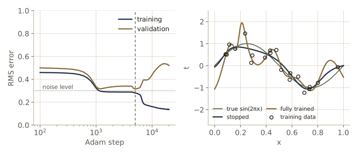
The validation error bottoms out at 0.315, close to the noise level, after 5,000 steps. By step 20,000 the training error has fallen further, to 0.135, well below the noise level, which is a sure sign of fitting the noise, and the validation error has risen to 0.52.
For a quadratic error, early stopping and weight decay are closely related. Rotate weight space to the eigenvectors of the Hessian and start at \(\mathbf{w} = \mathbf{0}\). Gradient descent moves fastest along the directions of high curvature, so after a few steps those components are nearly at their final values while the low-curvature components have barely moved. Weight decay has the same effect: it leaves well-determined, high-curvature directions nearly alone and shrinks poorly determined ones toward zero (the effective number of parameters of module 03). Working through the quadratic case shows that stopping after \(\tau\) steps of gradient descent with learning rate \(\eta\) acts roughly like weight decay with \(\lambda \approx 1/(\tau\eta)\) (exercise 8). So the effective number of parameters grows as training proceeds, and stopping early caps it.
Invariances
In many problems we know in advance that the prediction should not change, or should be invariant, when the input is transformed in certain ways. An object in an image keeps its class when it is shifted (translation invariance) or resized (scale invariance). A spoken word keeps its meaning when it is spoken a little faster or slower. Such transformations can change the raw input, the pixel intensities or the samples of the signal, enormously.
Given enough data, a flexible network can learn an invariance from examples, but that may take many examples of each transformation, and the number of combinations grows quickly when there are several transformations. There are four broad ways to help:
- Augment the training set with transformed copies of the training inputs, for instance shifted and slightly rotated digits.
- Add a regularizer that penalizes changes of the output under the transformation. This is tangent propagation, below.
- Preprocess the inputs into features that are already invariant. Any model built on such features inherits the invariance, and it holds even for transformations far larger than any in the training set; the difficulty is to find invariant features that do not also throw away information needed for the task.
- Build the invariance into the network’s structure, as convolutional networks do with local receptive fields and shared weights.
Augmentation is often the easiest. With stochastic training, each pass over the data can use freshly transformed copies; with batch training, each point is replicated several times with independent transformations. It can improve generalization a great deal, at the cost of more computation. The next two subsections show that approaches 1 and 2 are closely related.
Tangent propagation
Suppose a transformation of the input is governed by one continuous parameter \(\xi\), such as a rotation angle, and write \(\mathbf{s}(\mathbf{x}, \xi)\) for the transformed input, with \(\mathbf{s}(\mathbf{x}, 0) = \mathbf{x}\). As \(\xi\) varies, the input \(\mathbf{x}_n\) traces out a curve in input space. Its direction at \(\xi = 0\) is the tangent vector
\[\boldsymbol{\tau}_n = \left. \frac{\partial \mathbf{s}(\mathbf{x}_n, \xi)}{\partial \xi} \right\rvert_{\xi = 0} .\](The transformation must be continuous for this to make sense: rotations and shifts qualify, a mirror reflection does not.) The rate at which output \(k\) changes under the transformation is, by the chain rule, a Jacobian-vector product:
\[\left. \frac{\partial y_k}{\partial \xi} \right\rvert_{\xi = 0} = \sum_{i=1}^{D} \frac{\partial y_k}{\partial x_i} \frac{\partial x_i}{\partial \xi} = \sum_{i=1}^{D} J_{ki} \tau_i .\]Tangent propagation adds a penalty on these rates at the training points,
\[\widetilde{E} = E + \lambda \Omega, \qquad \Omega = \frac{1}{2} \sum_n \sum_k \left( \sum_{i=1}^{D} J_{nki} \tau_{ni} \right)^2 ,\]which is zero exactly when the network is locally invariant around every training point; \(\lambda\) trades fitting the data against learning the invariance. In practice the tangent vector is approximated by a finite difference, \(\boldsymbol{\tau}_n \approx \{\mathbf{s}(\mathbf{x}_n, \xi) - \mathbf{x}_n\}/\xi\) for a small \(\xi\), for example by rotating an image slightly and subtracting. The penalty depends on the weights through the Jacobian, and its gradient can be computed by an extension of backpropagation (Bishop’s exercise 5.26). For transformations with several parameters, such as shifts combined with rotations, add one such term per parameter. A related idea, tangent distance, builds the same invariances into nearest-neighbor classifiers.
Training with transformed data
Tangent propagation and data augmentation turn out to be nearly the same thing. Take one output and the sum-of-squares error, written in the large-data limit as \(E = \tfrac12 \iint \{y(\mathbf{x}) - t\}^2 p(t \mid \mathbf{x}) p(\mathbf{x}) \, d\mathbf{x} \, dt\), as in module 01. Now replace each input by a randomly transformed copy \(\mathbf{s}(\mathbf{x}, \xi)\), with \(\xi\) drawn from a distribution with mean zero and a small variance \(\lambda = \mathbb{E}[\xi^2]\). Expanding in powers of \(\xi\),
\[\mathbf{s}(\mathbf{x}, \xi) = \mathbf{x} + \xi \boldsymbol{\tau} + \frac{\xi^2}{2} \boldsymbol{\tau}' + O(\xi^3),\]where \(\boldsymbol{\tau}'\) is the second derivative of \(\mathbf{s}\) with respect to \(\xi\) at 0, and then expanding \(y(\mathbf{s}(\mathbf{x}, \xi))\) in the same way and averaging over \(\xi\), the terms linear in \(\xi\) drop out because \(\mathbb{E}[\xi] = 0\). What remains, to second order, is
\[\begin{aligned} \widetilde{E} &= E + \lambda \Omega, \\ \Omega &= \frac{1}{2} \int \Big[ \{ y(\mathbf{x}) - \mathbb{E}[t \mid \mathbf{x}] \} \left\{ (\boldsymbol{\tau}')^{\mathrm{T}} \nabla y(\mathbf{x}) + \boldsymbol{\tau}^{\mathrm{T}} \nabla\nabla y(\mathbf{x})\, \boldsymbol{\tau} \right\} \\ &\qquad\qquad + \left( \boldsymbol{\tau}^{\mathrm{T}} \nabla y(\mathbf{x}) \right)^2 \Big] p(\mathbf{x}) \, d\mathbf{x} . \end{aligned}\]The minimizer of \(\widetilde{E}\) is the conditional mean \(\mathbb{E}[t \mid \mathbf{x}]\) plus a correction of order \(\xi\), so the first term inside the brackets is of higher order and can be dropped. That leaves \(\Omega = \tfrac12 \int (\boldsymbol{\tau}^{\mathrm{T}} \nabla y)^2 p(\mathbf{x}) \, d\mathbf{x}\), which is the tangent propagation penalty. In the special case where the “transformation” is just added noise, \(\mathbf{x} \to \mathbf{x} + \boldsymbol{\xi}\), the penalty becomes
\[\Omega = \frac{1}{2} \int \lVert \nabla y(\mathbf{x}) \rVert^2 p(\mathbf{x}) \, d\mathbf{x},\]known as Tikhonov regularization. So training with a little input noise is, to leading order, the same as penalizing the slope of the network function.
We can check the expansion directly. For one input, the average of \(\tfrac12 \{y(x_n + \xi) - t_n\}^2\) over noise with variance \(\lambda\) is, to order \(\lambda\), the noise-free error plus \(\tfrac{\lambda}{2}\{y'(x_n)^2 + (y(x_n) - t_n) y''(x_n)\}\). We compare a Monte Carlo average with this formula, and with its Tikhonov part alone, for the two networks of the early-stopping experiment, with input noise of standard deviation 0.02.
def y_derivs(w, x, arch):
    """y(x), dy/dx, d2y/dx2 for a network with one input and one linear output."""
    W1, b1, W2, b2 = unpack(w, arch)
    Z = np.tanh(np.outer(x, W1[:, 0]) + b1)
    hp = 1 - Z ** 2
    y = Z @ W2[0] + b2[0]
    return y, (hp * W1[:, 0]) @ W2[0], (-2 * Z * hp * W1[:, 0] ** 2) @ W2[0]

x, t = X_tr[:, 0], T_tr[:, 0]
noise_sd = 0.02
lam = noise_sd ** 2
xi = np.random.default_rng(7).normal(0, noise_sd, (4000, len(x)))   # 4000 noisy copies
for name, w_net in [("stopped", w_stop), ("fully trained", w_end)]:
    y, dy, d2y = y_derivs(w_net, x, arch)
    E_clean = 0.5 * np.sum((y - t) ** 2)
    E_noisy = np.mean([0.5 * np.sum((y_derivs(w_net, x + row, arch)[0] - t) ** 2)
                       for row in xi])
    E_formula = E_clean + 0.5 * lam * np.sum(dy ** 2 + (y - t) * d2y)
    E_tikhonov = E_clean + 0.5 * lam * np.sum(dy ** 2)
    print(f"{name:14s} noise-free {E_clean:.4f}   Monte Carlo {E_noisy:.4f}"
          f"   formula {E_formula:.4f}   Tikhonov only {E_tikhonov:.4f}")
stopped        noise-free 0.7860   Monte Carlo 0.8670   formula 0.8667   Tikhonov only 0.8651
fully trained  noise-free 0.1829   Monte Carlo 0.7210   formula 0.7943   Tikhonov only 0.7800
For the smooth, early-stopped network, the second-order formula matches the Monte Carlo average to three decimals, and the Tikhonov term alone is nearly as good, since the fit is close to the conditional mean. For the overfitted network the expansion is off by about 10 percent: its function bends so sharply between the data points that a shift of 0.02 is no longer “small”. The equivalence between noise and a slope penalty holds only for noise that is small on the scale over which the network changes.
Convolutional networks
The fourth approach builds invariance into the architecture. The best-known example is the convolutional neural network, widely used for images. A fully connected network could in principle learn to recognize handwritten digits from the raw pixels, but it would ignore two facts about images: nearby pixels are much more strongly related than distant ones, and a feature that is useful in one part of an image (an edge, a corner, a loop) is likely to be useful everywhere.
A convolutional network uses three mechanisms. Local receptive fields: each unit in a convolutional layer looks only at a small patch of the input, say \(5 \times 5\) pixels. Weight sharing: the units are arranged in planes called feature maps, and all units in one feature map use the same weights, so they detect the same pattern at different positions. Computing a feature map is then a convolution of the image with a small kernel of weights, followed by the nonlinearity; if the input shifts, the feature map shifts with it but is otherwise unchanged. Subsampling: a following layer summarizes small, non-overlapping blocks of each feature map (for example \(2 \times 2\) blocks, halving the resolution), which makes its units insensitive to small shifts. Several pairs of convolution and subsampling layers can be stacked, with more feature maps at lower resolution in later stages, followed by a fully connected layer and a softmax output. Training uses backpropagation, adapted so that the gradients of all copies of a shared weight are added together (Bishop’s exercise 5.28).
The next cell shows the two effects in miniature: a feature map computed with one shared kernel shifts along with its input, and weight sharing collapses the number of free parameters.
signal = np.zeros(30)
signal[8:12] = [1.0, 2.0, 2.0, 1.0]
kernel = np.array([1.0, 0.0, -1.0])                      # one set of 3 shared weights
feature_map = lambda s: np.tanh(np.correlate(s, kernel, mode="valid"))
shifted = np.roll(signal, 5)
print("strongest response at position", np.argmax(feature_map(signal)),
      "-> after shifting the input by 5:", np.argmax(feature_map(shifted)))
print("shifted input gives the shifted map:",
      np.allclose(feature_map(shifted)[5:], feature_map(signal)[:-5]))

# 6 feature maps of 24 x 24 units on a 28 x 28 image, each unit seeing a 5 x 5 patch
units = 6 * 24 * 24
print(f"fully connected: {units * (28 * 28 + 1):,} parameters")
print(f"local receptive fields: {units * (25 + 1):,} parameters")
print(f"local fields with shared weights: {6 * (25 + 1)} parameters")
strongest response at position 10 -> after shifting the input by 5: 15
shifted input gives the shifted map: True
fully connected: 2,712,960 parameters
local receptive fields: 89,856 parameters
local fields with shared weights: 156 parameters
Soft weight sharing
Hard weight sharing requires knowing in advance which weights should be equal. Soft weight sharing replaces the hard constraint by a regularizer that encourages weights to form groups of similar values, and learns the groups, their centers, and their spreads along with the weights. Recall that weight decay is the negative log of a single zero-mean Gaussian prior. Replace that prior by a mixture of Gaussians (module 02 and module 09), independently for each weight:
\[p(\mathbf{w}) = \prod_i \sum_{j=1}^{M} \pi_j \mathcal{N}(w_i \mid \mu_j, \sigma_j^2), \qquad \Omega(\mathbf{w}) = -\sum_i \ln \left( \sum_{j=1}^{M} \pi_j \mathcal{N}(w_i \mid \mu_j, \sigma_j^2) \right),\]and minimize \(\widetilde{E} = E + \lambda\Omega\) over the weights and the mixture parameters together. (Running EM on the mixture while the weights are still moving tends to be unstable, so the joint minimization uses a general-purpose optimizer.) With the responsibilities \(\gamma_j(w) = \pi_j \mathcal{N}(w \mid \mu_j, \sigma_j^2) / \sum_k \pi_k \mathcal{N}(w \mid \mu_k, \sigma_k^2)\), the gradient with respect to a weight is
\[\frac{\partial \widetilde{E}}{\partial w_i} = \frac{\partial E}{\partial w_i} + \lambda \sum_j \gamma_j(w_i) \frac{w_i - \mu_j}{\sigma_j^2} ,\]so each weight is pulled toward the centers of the components that claim it, in proportion to how strongly they claim it. The centers in turn move toward the responsibility-weighted average of the weights, and the variances toward the weighted spread. To keep the parameters valid, one optimizes \(\ln \sigma_j^2\) instead of \(\sigma_j^2\) and represents the \(\pi_j\) by a softmax of free variables; the gradient with respect to those variables is \(\lambda \sum_i \{\pi_j - \gamma_j(w_i)\}\), which drives each \(\pi_j\) toward the average responsibility of component \(j\). Bishop §5.5.7 gives all the derivatives.
Mixture density networks
The problem with least squares
Supervised learning is really about the conditional distribution \(p(t \mid \mathbf{x})\). For many regression problems a Gaussian with a mean that depends on \(\mathbf{x}\) is a fine model, and least squares fits exactly that. But some problems have conditional distributions that are far from Gaussian, and the typical source is an inverse problem. A robot arm with two joints is a good picture. Given the joint angles, the position of the hand is determined uniquely; that is the forward problem. But to put the hand at a given position we need the inverse, and a two-joint arm can usually reach a point in two ways, with the elbow bent up or bent down. The average of the two solutions is generally not a solution at all. Whenever the forward map is many-to-one, the inverse map is one-to-many, and \(p(t \mid \mathbf{x})\) is multimodal.
A small version is easy to generate. Draw \(x\) uniformly on \((0, 1)\), set \(t = x + 0.3 \sin(2\pi x)\) plus uniform noise on \((-0.1, 0.1)\); that is a forward problem with one value of \(t\) for each \(x\). Now swap the roles of the two variables. For inputs near the middle of the range there are three branches of targets. We fit an ordinary least-squares network with six hidden units to both problems.
def toy_data(N, rng):
    """Forward problem: x uniform on (0, 1), t = x + 0.3 sin(2 pi x) + uniform noise."""
    x = rng.uniform(0, 1, N)
    return x, x + 0.3 * np.sin(2 * np.pi * x) + rng.uniform(-0.1, 0.1, N)

rng_md = np.random.default_rng(2)
x_f, t_f = toy_data(200, rng_md)
arch_ls = (1, 6, 1)
for name, inputs, targets in [("forward", x_f, t_f), ("inverse", t_f, x_f)]:
    X, T = inputs[:, None], targets[:, None]
    w_ls = adam(lambda v: backprop(v, X, T, arch_ls), init_weights(arch_ls, rng_md),
                3000, lr=0.02)
    print(f"{name}: least-squares RMS error {rms(w_ls, X, T, arch_ls):.3f}")
X_inv, t_inv = t_f[:, None], x_f              # the inverse problem: predict x_f from t_f
w_ls_inv = w_ls
near = np.abs(X_inv[:, 0] - 0.6) < 0.02
y_06 = forward(w_ls_inv, np.array([[0.6]]), arch_ls)[2][0, 0]
print(f"inverse problem, input 0.6: least squares predicts {y_06:.3f}")
print("targets with inputs within 0.02 of 0.6:", np.round(np.sort(t_inv[near]), 2))
forward: least-squares RMS error 0.055
inverse: least-squares RMS error 0.189
inverse problem, input 0.6: least squares predicts 0.491
targets with inputs within 0.02 of 0.6: [0.27 0.29 0.39 0.41 0.43 0.78 0.83]
The forward fit is about as good as the noise allows (uniform noise on \((-0.1, 0.1)\) has standard deviation 0.058). The inverse fit is much worse, and its prediction at input 0.6, about 0.49, falls in the gap between two groups of targets, one near 0.3 to 0.4 and one near 0.8, where there are no training targets at all. Least squares is maximum likelihood for a Gaussian, whose mean is the best single guess under squared error; here the best single guess is an average of the branches, which is rarely right.
The model
A mixture density network (MDN) models the conditional density as a mixture whose parameters are all functions of the input, computed by a neural network:
\[p(t \mid \mathbf{x}) = \sum_{k=1}^{K} \pi_k(\mathbf{x})\, \mathcal{N}\left(t \mid \mu_k(\mathbf{x}), \sigma_k^2(\mathbf{x})\right).\]For each input the mixture can be unimodal or multimodal, broad or narrow; it is heteroscedastic, since the noise level may depend on \(\mathbf{x}\). With a flexible enough network and enough components, it can approximate essentially any conditional density. The components need not be Gaussian (Bernoulli components suit binary targets), and for a vector target the Gaussians can have full covariance matrices; we use a scalar target to keep the notation simple. It is a close relative of the mixture of experts of module 14; the difference is that here one network, with shared hidden units, computes the parameters of all components.
The network has \(3K\) outputs for a scalar target (for a \(D_t\)-dimensional target with isotropic components, \((D_t + 2)K\)), and each group gets an output activation that respects its constraints:
- mixing coefficients, which must be positive and sum to 1: a softmax, \(\pi_k = \exp(a^{\pi}_k) / \sum_l \exp(a^{\pi}_l)\);
- standard deviations, which must be positive: \(\sigma_k = \exp(a^{\sigma}_k)\);
- means, which can be any real number: \(\mu_k = a^{\mu}_k\).
The error is the negative log likelihood,
\[E(\mathbf{w}) = -\sum_{n=1}^{N} \ln \left\{ \sum_{k=1}^{K} \pi_k(\mathbf{x}_n, \mathbf{w})\, \mathcal{N}\left(t_n \mid \mu_k(\mathbf{x}_n, \mathbf{w}), \sigma_k^2(\mathbf{x}_n, \mathbf{w})\right) \right\}.\]Gradients for backpropagation
To train with backpropagation we need only the output errors \(\partial E_n / \partial a\) for the \(3K\) output activations; the backward pass through the hidden layer is unchanged. As in the EM algorithm for mixtures, it helps to read \(\pi_k(\mathbf{x})\) as a prior probability of component \(k\) and to define the responsibilities
\[\gamma_{nk} = \frac{\pi_k \mathcal{N}_{nk}}{\sum_{l} \pi_l \mathcal{N}_{nl}}, \qquad \mathcal{N}_{nk} = \mathcal{N}\left(t_n \mid \mu_k(\mathbf{x}_n), \sigma_k^2(\mathbf{x}_n)\right).\]For the mixing coefficients, \(\partial E_n / \partial \pi_j = -\mathcal{N}_{nj} / \sum_l \pi_l \mathcal{N}_{nl} = -\gamma_{nj} / \pi_j\), and the softmax derivatives are \(\partial \pi_j / \partial a^{\pi}_k = \pi_j (I_{jk} - \pi_k)\), so
\[\frac{\partial E_n}{\partial a^{\pi}_k} = -\sum_j \frac{\gamma_{nj}}{\pi_j} \pi_j (I_{jk} - \pi_k) = \pi_k - \gamma_{nk} .\]For the means and the widths, use \(\ln \mathcal{N}_{nk} = -\tfrac12 \ln(2\pi) - \ln\sigma_k - (t_n - \mu_k)^2 / (2\sigma_k^2)\) with \(\ln\sigma_k = a^{\sigma}_k\), and \(\partial E_n / \partial \ln \mathcal{N}_{nk} = -\gamma_{nk}\):
\[\frac{\partial E_n}{\partial a^{\mu}_k} = \gamma_{nk} \frac{\mu_k - t_n}{\sigma_k^2}, \qquad \frac{\partial E_n}{\partial a^{\sigma}_k} = \gamma_{nk} \left\{ 1 - \frac{(t_n - \mu_k)^2}{\sigma_k^2} \right\}.\]These are pleasant to read. The mixing coefficient of a component rises when its responsibility exceeds its prior. The mean of a component moves toward the target, weighted by its responsibility. Its width grows when the target is more than one standard deviation away and shrinks otherwise. (For a \(D_t\)-dimensional target the 1 in the last formula becomes \(D_t\).) In code, all quantities are computed in log space, with the responsibilities from a log-sum-exp.
def mdn_params(A2, K):
    """Split the 3K output activations into log pi_k, log sigma_k, and mu_k."""
    a_pi, a_sigma, mu = A2[:, :K], A2[:, K:2 * K], A2[:, 2 * K:]
    return a_pi - logsumexp(a_pi, axis=1, keepdims=True), a_sigma, mu

def mdn_backprop(w, X, t, arch):
    """Negative log likelihood of a mixture density network and its gradient."""
    K = arch[2] // 3
    A1, Z, A2 = forward(w, X, arch)
    log_pi, log_sigma, mu = mdn_params(A2, K)
    r2 = (t[:, None] - mu) ** 2 / np.exp(2 * log_sigma)      # (t - mu_k)^2 / sigma_k^2
    log_joint = log_pi - 0.5 * np.log(2 * np.pi) - log_sigma - 0.5 * r2
    log_p = logsumexp(log_joint, axis=1, keepdims=True)
    gamma = np.exp(log_joint - log_p)                        # responsibilities gamma_nk
    d2 = np.hstack([np.exp(log_pi) - gamma,                  # dE/da_pi = pi_k - gamma_k
                    gamma * (1 - r2),                        # dE/da_sigma
                    gamma * (mu - t[:, None]) / np.exp(2 * log_sigma)])   # dE/da_mu
    return -np.sum(log_p), backward(w, X, Z, d2, arch)

K = 3
arch_mdn = (1, 6, 3 * K)
w = init_weights(arch_mdn, rng_md)
E, g = mdn_backprop(w, X_inv[:20], t_inv[:20], arch_mdn)
E_20 = lambda v: mdn_backprop(v, X_inv[:20], t_inv[:20], arch_mdn)[0]  # 20 points
g_num = numerical_gradient(E_20, w)
print(f"W = {w.size}   max relative error vs central differences:"
      f" {max_rel_error(g, g_num):.1e}")
W = 75 max relative error vs central differences: 1.8e-07
Fitting the inverse problem
We train an MDN with three components and six hidden units on the 200 points of the inverse problem, and compare it with the least-squares network on 1,000 fresh test points. To compare two probabilistic models fairly, we use the average log likelihood of the test targets; for the least-squares network that means a Gaussian around its prediction with the maximum likelihood noise level \(1/\beta_{\mathrm{ML}}\) from the training data.
w_mdn = adam(lambda v: mdn_backprop(v, X_inv, t_inv, arch_mdn), w, 3000, lr=0.02)

x_test, t_test = toy_data(1000, rng_md)
X_te, t_te = t_test[:, None], x_test                    # inverse problem again
var_ml = 2 * backprop(w_ls_inv, X_inv, t_inv[:, None], arch_ls)[0] / len(t_inv)  # 1/beta
y_te = forward(w_ls_inv, X_te, arch_ls)[2][:, 0]
ll_ls = np.mean(-0.5 * np.log(2 * np.pi * var_ml) - (t_te - y_te) ** 2 / (2 * var_ml))
ll_mdn = -mdn_backprop(w_mdn, X_te, t_te, arch_mdn)[0] / len(t_te)
print(f"test log likelihood per point:  least squares {ll_ls:.3f}"
      f"   mixture density network {ll_mdn:.3f}")

x_show = np.array([[0.1], [0.5], [0.9]])
log_pi, log_sigma, mu = mdn_params(forward(w_mdn, x_show, arch_mdn)[2], K)
for x0, p, m, s in zip(x_show[:, 0], np.exp(log_pi), mu, np.exp(log_sigma)):
    print(f"input {x0}:  pi {p.round(3)}   mu {m.round(3)}   sigma {s.round(3)}")
test log likelihood per point:  least squares 0.170   mixture density network 1.026
input 0.1:  pi [0.998 0.    0.002]   mu [0.047 0.524 0.438]   sigma [0.014 0.    0.013]
input 0.5:  pi [0.238 0.582 0.181]   mu [0.227 0.517 0.775]   sigma [0.035 0.08  0.04 ]
input 0.9:  pi [0.036 0.011 0.953]   mu [0.489 0.009 0.959]   sigma [0.087 0.014 0.016]
The MDN assigns the test targets a far higher likelihood than the Gaussian of least squares: 1.03 against 0.17 per point, on the log scale. The component parameters show how. At an input of 0.5, inside the three-branch region, all three mixing coefficients are substantial and the three means, 0.23, 0.52, and 0.78, sit on the three branches (the noise-free branches are at 0.21, 0.5, and 0.79). At 0.1 and 0.9, where the targets form a single branch, one component carries 95 percent of the weight or more.
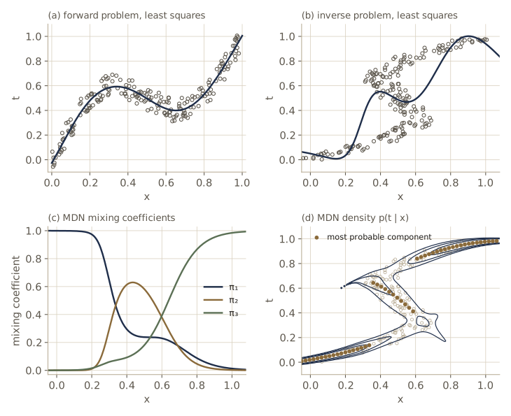
The network’s outputs are smooth, single-valued functions of the input, yet the density they describe changes from one mode to three and back, simply by shifting the mixing coefficients. Once trained, an MDN gives the whole conditional density, and any summary we need follows from it. The conditional mean is
\[\mathbb{E}[t \mid \mathbf{x}] = \sum_{k=1}^{K} \pi_k(\mathbf{x}) \mu_k(\mathbf{x}),\]which is what least squares estimates, so an MDN contains the least-squares answer as a special case. The conditional variance, which now depends on \(\mathbf{x}\), is
\[s^2(\mathbf{x}) = \sum_{k=1}^{K} \pi_k(\mathbf{x}) \left\{ \sigma_k^2(\mathbf{x}) + \left( \mu_k(\mathbf{x}) - \sum_{l=1}^{K} \pi_l(\mathbf{x}) \mu_l(\mathbf{x}) \right)^2 \right\}.\]For a multimodal density the mean is of little use (for the robot arm it is not a valid arm position), and the conditional mode is more useful. It has no closed form, but a simple stand-in is the mean of the component with the largest mixing coefficient, which is what panel (d) shows.
x_grid = np.array([[0.1], [0.5], [0.9]])
log_pi, log_sigma, mu = mdn_params(forward(w_mdn, x_grid, arch_mdn)[2], K)
pi, sigma = np.exp(log_pi), np.exp(log_sigma)
mean = np.sum(pi * mu, axis=1)                                         # E[t | x]
var = np.sum(pi * (sigma ** 2 + (mu - mean[:, None]) ** 2), axis=1)   # s^2(x)
mode = mu[np.arange(len(x_grid)), np.argmax(pi, axis=1)]  # most probable component
print("conditional mean:        ", mean)
print("conditional std:         ", np.sqrt(var))
print("most probable component: ", mode)
print("least squares:           ", forward(w_ls_inv, x_grid, arch_ls)[2][:, 0])
conditional mean:         [0.0482 0.4949 0.9315]
conditional std:          [0.022  0.1893 0.1335]
most probable component:  [0.0474 0.5174 0.959 ]
least squares:            [0.0166 0.4863 1.0018]
At 0.1 the mean and the approximate mode agree. At 0.5 the conditional mean is close to the least-squares prediction, as it should be, and the conditional standard deviation of 0.19 reveals that the mean is a poor summary there. At 0.9, a component with only 4 percent of the weight but a far-off mean pulls the conditional mean below the mode and inflates the standard deviation to 0.13. Means and variances of mixtures are sensitive to small, distant components; the mode is not.
Bayesian neural networks
So far we have fitted networks by maximum likelihood, or by penalized maximum likelihood, which is MAP estimation with the penalty as a log prior. A Bayesian treatment instead averages predictions over the posterior distribution of the weights. For linear regression in module 03 this was exact, because the posterior was Gaussian. For a network, the output is a nonlinear function of the weights, the posterior is not Gaussian, and it is multimodal, since the error has many minima. Variational methods (module 10) and Markov chain Monte Carlo (module 11) are both used. Here we follow the most developed analytic approach, based on the Laplace approximation, and make two simplifications: approximate the posterior by a Gaussian around one mode, and assume that this Gaussian is narrow enough for the network to be nearly linear in the weights across it. With these, the network behaves locally like the linear models of modules 03 and 04, and we can reuse their results.
Posterior parameter distribution
Take one real target with Gaussian noise of precision \(\beta\) and an isotropic Gaussian prior with precision \(\alpha\):
\[p(t \mid \mathbf{x}, \mathbf{w}, \beta) = \mathcal{N}\left(t \mid y(\mathbf{x}, \mathbf{w}), \beta^{-1}\right), \qquad p(\mathbf{w} \mid \alpha) = \mathcal{N}(\mathbf{w} \mid \mathbf{0}, \alpha^{-1}\mathbf{I}).\]For a data set \(\mathcal{D} = \{t_1, \dots, t_N\}\) with inputs \(\mathbf{x}_1, \dots, \mathbf{x}_N\), the log posterior is
\[\ln p(\mathbf{w} \mid \mathcal{D}) = -\frac{\alpha}{2} \mathbf{w}^{\mathrm{T}}\mathbf{w} - \frac{\beta}{2} \sum_{n=1}^{N} \{ y(\mathbf{x}_n, \mathbf{w}) - t_n \}^2 + \text{const},\]a regularized sum-of-squares error with weight decay \(\lambda = \alpha/\beta\). Its maximum \(\mathbf{w}_{\mathrm{MAP}}\) is found by numerical optimization with backpropagated gradients. The Laplace approximation (module 04) then uses the curvature of the negative log posterior at the mode,
\[\mathbf{A} = -\nabla\nabla \ln p(\mathbf{w} \mid \mathcal{D}, \alpha, \beta) = \alpha \mathbf{I} + \beta \mathbf{H},\]where \(\mathbf{H}\) is the Hessian of the sum-of-squares error \(\tfrac12\sum_n (y_n - t_n)^2\), to give a Gaussian approximate posterior
\[q(\mathbf{w} \mid \mathcal{D}) = \mathcal{N}\left(\mathbf{w} \mid \mathbf{w}_{\mathrm{MAP}}, \mathbf{A}^{-1}\right).\]The predictive distribution integrates the likelihood against the posterior,
\[p(t \mid \mathbf{x}, \mathcal{D}) = \int p(t \mid \mathbf{x}, \mathbf{w})\, q(\mathbf{w} \mid \mathcal{D}) \, d\mathbf{w},\]which is still intractable because \(y\) is nonlinear in \(\mathbf{w}\). Now use the second simplification: if the posterior is narrow compared with the scale on which \(y\) changes with \(\mathbf{w}\), linearize the network around the mode,
\[y(\mathbf{x}, \mathbf{w}) \approx y(\mathbf{x}, \mathbf{w}_{\mathrm{MAP}}) + \mathbf{g}^{\mathrm{T}} (\mathbf{w} - \mathbf{w}_{\mathrm{MAP}}),\]where \(\mathbf{g} = \nabla_{\mathbf{w}} y(\mathbf{x}, \mathbf{w})\) is the gradient of the network output with respect to the weights, evaluated at \(\mathbf{w}_{\mathrm{MAP}}\). The target is then a linear-Gaussian function of a Gaussian weight vector, and the marginalization result for linear-Gaussian models from module 02 gives
\[p(t \mid \mathbf{x}, \mathcal{D}, \alpha, \beta) = \mathcal{N}\left(t \mid y(\mathbf{x}, \mathbf{w}_{\mathrm{MAP}}), \sigma^2(\mathbf{x})\right), \qquad \sigma^2(\mathbf{x}) = \beta^{-1} + \mathbf{g}^{\mathrm{T}} \mathbf{A}^{-1} \mathbf{g} .\]Result. The predictive mean is the MAP network’s output. The predictive variance has two parts: the noise \(\beta^{-1}\), and a term \(\mathbf{g}^{\mathrm{T}}\mathbf{A}^{-1}\mathbf{g}\) that measures how uncertain the weights make the output at this particular \(\mathbf{x}\). It has the same form as the predictive variance of Bayesian linear regression in module 03, with the basis-function vector replaced by the gradient \(\mathbf{g}\) of the network output.
The vector \(\mathbf{g}\) is exactly the \(\mathbf{b}_n\) of the outer-product approximation, evaluated at a new input, so output_grads computes it. We take 30 noisy points from \(\sin(2\pi x)\) with a gap in the middle of the input range, and fit a network with six hidden units at starting values \(\alpha = 0.1\) and \(\beta = 10\). Since fit_lm minimizes \(E + \tfrac12 \sum_i r_i w_i^2\), we pass \(r_i = \alpha/\beta\). For \(\mathbf{H}\) we compute the exact Hessian (by hessian_fd) and the outer-product approximation, and compare the error bars they give.
rng_b = np.random.default_rng(3)
x = np.concatenate([rng_b.uniform(0, 0.35, 15), rng_b.uniform(0.65, 1, 15)])
X_b, T_b = x[:, None], (np.sin(2 * np.pi * x) + rng_b.normal(0, 0.2, 30))[:, None]
arch_b = (1, 6, 1)
N_b, W_b = len(X_b), n_weights(arch_b)
alpha, beta = 0.1, 10.0
w_map = fit_lm(init_weights(arch_b, rng_b), X_b, T_b, arch_b, r=alpha / beta)

def predictive(w, X_new, A, beta):
    """Laplace predictive mean and standard deviation: sigma^2 = 1/beta + g^T A^(-1) g."""
    G = output_grads(w, X_new, arch_b)                     # rows g(x)
    var = 1 / beta + np.sum(G * np.linalg.solve(A, G.T).T, axis=1)
    return forward(w, X_new, arch_b)[2][:, 0], np.sqrt(var)

H_exact = hessian_fd(lambda v: backprop(v, X_b, T_b, arch_b)[1], w_map)
B_b = output_grads(w_map, X_b, arch_b)
X_new = np.array([[0.1], [0.5], [0.9], [1.3]])
for name, Hm in [("exact Hessian", H_exact), ("outer product", B_b.T @ B_b)]:
    mean, sd = predictive(w_map, X_new, alpha * np.eye(W_b) + beta * Hm, beta)
    print(f"{name:14s} mean {mean}   sd {sd}")
print(f"noise alone: sd {1 / np.sqrt(beta):.4f}")
exact Hessian  mean [ 0.5103  0.0655 -0.5929  0.8273]   sd [0.3326 0.5429 0.3319 0.7996]
outer product  mean [ 0.5103  0.0655 -0.5929  0.8273]   sd [0.3339 0.5426 0.3326 0.9329]
noise alone: sd 0.3162
Near the data (inputs 0.1 and 0.9) the predictive standard deviation is barely above the noise level. In the gap (0.5), and even more outside the data (1.3), the weight uncertainty adds a large term. The exact and outer-product Hessians give nearly the same error bars near the data and in the gap, as expected for a trained network; they differ more at 1.3 (0.80 against 0.93), far outside the data, where the linearization is least trustworthy anyway.
Hyperparameter optimization
We fixed \(\alpha\) and \(\beta\) by hand. As in module 03, we can instead choose them by maximizing the evidence \(p(\mathcal{D} \mid \alpha, \beta) = \int p(\mathcal{D} \mid \mathbf{w}, \beta) p(\mathbf{w} \mid \alpha) \, d\mathbf{w}\). The Laplace approximation of the integral (module 04) gives
\[\ln p(\mathcal{D} \mid \alpha, \beta) \approx -E(\mathbf{w}_{\mathrm{MAP}}) - \frac{1}{2} \ln \lvert \mathbf{A} \rvert + \frac{W}{2} \ln\alpha + \frac{N}{2} \ln\beta - \frac{N}{2} \ln(2\pi),\]with the regularized error \(E(\mathbf{w}_{\mathrm{MAP}}) = \tfrac{\beta}{2} \sum_n \{y(\mathbf{x}_n, \mathbf{w}_{\mathrm{MAP}}) - t_n\}^2 + \tfrac{\alpha}{2} \mathbf{w}_{\mathrm{MAP}}^{\mathrm{T}} \mathbf{w}_{\mathrm{MAP}}\). This has the same form as for linear regression, and maximizing it gives the same re-estimation equations. With the eigenvalues \(\lambda_i\) of \(\beta\mathbf{H}\),
\[\gamma = \sum_{i=1}^{W} \frac{\lambda_i}{\alpha + \lambda_i}, \qquad \alpha = \frac{\gamma}{\mathbf{w}_{\mathrm{MAP}}^{\mathrm{T}} \mathbf{w}_{\mathrm{MAP}}},\] \[\frac{1}{\beta} = \frac{1}{N - \gamma} \sum_{n=1}^{N} \{ y(\mathbf{x}_n, \mathbf{w}_{\mathrm{MAP}}) - t_n \}^2 ,\]where \(\gamma\) is the effective number of well-determined parameters. For a network these equations are approximate even within the Laplace approximation: changing \(\alpha\) moves \(\mathbf{w}_{\mathrm{MAP}}\) and so changes \(\mathbf{H}\) and its eigenvalues, and the derivation ignores that dependence. As in module 03, we alternate between re-estimating \(\alpha\) and \(\beta\) and re-fitting \(\mathbf{w}_{\mathrm{MAP}}\).
For the eigenvalues we use the outer-product Hessian. It is positive semidefinite, so every \(\lambda_i \ge 0\) and \(0 \le \gamma \le W\); the exact Hessian of the unregularized error can have negative eigenvalues even at a mode of the posterior, which would make \(\gamma\) meaningless.
def log_evidence(w, alpha, beta, H):
    """Laplace approximation to ln p(D | alpha, beta)."""
    E_reg = beta * backprop(w, X_b, T_b, arch_b)[0] + 0.5 * alpha * w @ w
    logdet = np.linalg.slogdet(alpha * np.eye(W_b) + beta * H)[1]
    return -E_reg - 0.5 * logdet + 0.5 * W_b * np.log(alpha) + 0.5 * N_b * np.log(beta) \
           - 0.5 * N_b * np.log(2 * np.pi)

for it in range(6):
    H_op = output_grads(w_map, X_b, arch_b).T @ output_grads(w_map, X_b, arch_b)
    lam = np.linalg.eigvalsh(beta * H_op)
    gamma = np.sum(lam / (alpha + lam))
    print(f"iteration {it}:  alpha {alpha:.4f}   beta {beta:6.3f}   gamma {gamma:.2f}"
          f"   ln evidence {log_evidence(w_map, alpha, beta, H_op):7.3f}")
    E_D = backprop(w_map, X_b, T_b, arch_b)[0]
    alpha, beta = gamma / (w_map @ w_map), (N_b - gamma) / (2 * E_D)
    w_map = fit_lm(w_map, X_b, T_b, arch_b, r=alpha / beta)
iteration 0:  alpha 0.1000   beta 10.000   gamma 5.15   ln evidence -16.602
iteration 1:  alpha 0.1087   beta 24.178   gamma 5.53   ln evidence -13.292
iteration 2:  alpha 0.1106   beta 24.224   gamma 5.52   ln evidence -13.283
iteration 3:  alpha 0.1106   beta 24.223   gamma 5.52   ln evidence -13.283
iteration 4:  alpha 0.1106   beta 24.223   gamma 5.52   ln evidence -13.283
iteration 5:  alpha 0.1106   beta 24.223   gamma 5.52   ln evidence -13.283
The iteration settles within a few rounds, and the log evidence rises from −16.6 to −13.3. The re-estimated \(\beta \approx 24.2\) corresponds to a noise standard deviation of \(24.2^{-1/2} \approx 0.20\), matching the 0.2 used to generate the data, and only \(\gamma \approx 5.5\) of the 19 parameters count as well determined. The figure shows the resulting predictive distribution.
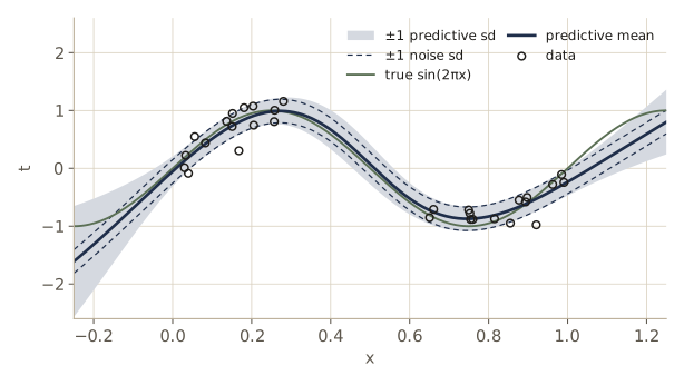
Two cautions apply to the evidence for networks. First, the posterior has many modes, and the \(\mathbf{w}_{\mathrm{MAP}}\) we find depends on the starting point. Modes related by the weight-space symmetries give identical predictions, so it does not matter which of them we find; but inequivalent modes give different hyperparameters and different evidence. Second, comparing networks with different numbers of hidden units by their evidence requires the evidence of the whole posterior, not of one mode. Since each mode comes with \(2^M M!\) equivalent copies, the evidence of one mode should be multiplied by \(2^M M!\) (exercise 10). Also, \(\ln \lvert\mathbf{A}\rvert\) is sensitive to small eigenvalues, which are hard to compute accurately; this makes the evidence less reliable than the re-estimated \(\alpha\) and \(\beta\), which depend on the eigenvalues only through \(\gamma\).
Bayesian neural networks for classification
For two-class classification with a single sigmoid output, the same program goes through with the changes we saw for logistic regression in module 04. There is no noise precision, since labels are assumed correct. The MAP weights minimize
\[E(\mathbf{w}) = -\sum_{n=1}^{N} \{ t_n \ln y_n + (1 - t_n) \ln(1 - y_n) \} + \frac{\alpha}{2} \mathbf{w}^{\mathrm{T}}\mathbf{w},\]and \(\mathbf{A} = \alpha\mathbf{I} + \mathbf{H}\), with \(\mathbf{H}\) the Hessian of the cross-entropy, exact or in the outer-product form \(\sum_n y_n(1 - y_n)\mathbf{b}_n\mathbf{b}_n^{\mathrm{T}}\). The evidence is \(\ln p(\mathcal{D} \mid \alpha) \approx -E(\mathbf{w}_{\mathrm{MAP}}) - \tfrac12 \ln\lvert\mathbf{A}\rvert + \tfrac{W}{2}\ln\alpha + \text{const}\), and maximizing it gives the same update \(\alpha = \gamma / \mathbf{w}_{\mathrm{MAP}}^{\mathrm{T}}\mathbf{w}_{\mathrm{MAP}}\).
For the predictive distribution, linearizing the output \(y\) would be a poor idea, because a linear function does not stay between 0 and 1. Instead we linearize the output activation,
\[a(\mathbf{x}, \mathbf{w}) \approx a_{\mathrm{MAP}}(\mathbf{x}) + \mathbf{b}^{\mathrm{T}} (\mathbf{w} - \mathbf{w}_{\mathrm{MAP}}), \qquad \mathbf{b} = \nabla_{\mathbf{w}} a(\mathbf{x}, \mathbf{w}_{\mathrm{MAP}}),\]so that under the Gaussian posterior the activation is Gaussian, with mean \(a_{\mathrm{MAP}}(\mathbf{x})\) and variance \(\sigma_a^2(\mathbf{x}) = \mathbf{b}^{\mathrm{T}}\mathbf{A}^{-1}\mathbf{b}\). The predictive probability is the sigmoid averaged over that Gaussian, which has no closed form; the probit approximation of module 04 gives
\[p(t = 1 \mid \mathbf{x}, \mathcal{D}) = \int \sigma(a)\, \mathcal{N}\left(a \mid a_{\mathrm{MAP}}, \sigma_a^2\right) da \approx \sigma\left( \kappa(\sigma_a^2)\, a_{\mathrm{MAP}} \right),\]with \(\kappa(\sigma^2) = (1 + \pi \sigma^2 / 8)^{-1/2}\).
The decision boundary, where \(a_{\mathrm{MAP}} = 0\), does not move; but wherever the activation is uncertain, the predicted probability is pulled toward 0.5. We try this on two Gaussian classes, check the approximation against an accurate numerical integral (Gauss–Hermite quadrature), and look at four test points.
rng_k = np.random.default_rng(8)
X_k = np.vstack([rng_k.normal([-1.0, 0.0], 0.7, (20, 2)),     # class 0
                 rng_k.normal([1.0, 0.0], 0.7, (20, 2))])     # class 1
T_k = np.repeat([0.0, 1.0], 20)[:, None]
arch_k, alpha_k = (2, 4, 1), 1.0
cross_entropy = lambda v: backprop(v, X_k, T_k, arch_k, "sigmoid")

def regularized(v):
    E, g = cross_entropy(v)
    return E + 0.5 * alpha_k * v @ v, g + alpha_k * v

w_k = adam(regularized, init_weights(arch_k, rng_k), 4000, lr=0.02)
A_k = alpha_k * np.eye(w_k.size) + hessian_fd(lambda v: cross_entropy(v)[1], w_k)

gh_nodes, gh_weights = np.polynomial.hermite_e.hermegauss(40)  # for N(0, 1) integrals
X_test = np.array([[1.0, 0.0], [0.0, 0.0], [0.0, 4.0], [4.0, 0.0]])
a_map = forward(w_k, X_test, arch_k)[2][:, 0]
Bk = output_grads(w_k, X_test, arch_k)                          # rows b(x)
sd_a = np.sqrt(np.sum(Bk * np.linalg.solve(A_k, Bk.T).T, axis=1))  # sqrt(b^T A^-1 b)
kappa = 1 / np.sqrt(1 + np.pi * sd_a ** 2 / 8)
for x0, a0, s, k in zip(X_test, a_map, sd_a, kappa):
    quad = np.sum(gh_weights * expit(a0 + s * gh_nodes)) / np.sqrt(2 * np.pi)
    print(f"x = {x0}:  a_MAP {a0:5.2f}  sd_a {s:4.2f}   p_MAP {expit(a0):.3f}"
          f"   moderated {expit(k * a0):.3f}   quadrature {quad:.3f}")
x = [1. 0.]:  a_MAP  2.93  sd_a 0.95   p_MAP 0.949   moderated 0.925   quadrature 0.928
x = [0. 0.]:  a_MAP  0.09  sd_a 0.75   p_MAP 0.523   moderated 0.521   quadrature 0.520
x = [0. 4.]:  a_MAP -2.86  sd_a 2.38   p_MAP 0.054   moderated 0.169   quadrature 0.167
x = [4. 0.]:  a_MAP  4.28  sd_a 1.29   p_MAP 0.986   moderated 0.965   quadrature 0.972
At the center of a class the activation is well determined and the moderated probability is close to the MAP value. Far from the training data, the activation is large but uncertain, and marginalizing over the weights pulls the probability back toward 0.5: the Bayesian network is appropriately less confident where it has seen no data. The probit approximation agrees with the numerical integral to within 0.01.
Summary
| Tool | What it does | Cost or key formula |
|---|---|---|
| Two-layer network | adaptive basis functions \(z_j = h(\sum_i w_{ji} x_i)\), matched output \(f\) | \(W = M(D+1) + K(M+1)\) parameters; \(2^M M!\) equivalent weight vectors |
| Matched output and error | identity / sum of squares, sigmoid / cross-entropy, softmax / cross-entropy | \(\partial E_n / \partial a_k = y_k - t_k\) |
| Backpropagation | gradient of the error for any feed-forward network | \(\delta_j = h'(a_j)\sum_k w_{kj}\delta_k\), \(\partial E_n/\partial w_{ji} = \delta_j z_i\); \(O(W)\) |
| Finite differences | check of any derivative code | central differences, error \(O(\epsilon^2)\); \(O(W^2)\) for a gradient |
| Jacobian | sensitivity of outputs to inputs | backward recursion for \(\partial y_k / \partial a_j\) |
| Hessian approximations | curvature for optimization, pruning, Laplace | diagonal \(O(W)\); outer product \(\sum_n \mathbf{b}_n\mathbf{b}_n^{\mathrm{T}}\); exact \(O(W^2)\); \(\mathbf{H}\mathbf{v}\) in \(O(W)\) |
| Regularization | control complexity | weight decay, consistent per-layer priors, early stopping, invariances |
| Mixture density network | multimodal \(p(t \mid \mathbf{x})\) | outputs set \(\pi_k, \mu_k, \sigma_k\); output errors \(\pi_k - \gamma_k\) and relatives |
| Laplace Bayesian network | error bars and hyperparameters | \(\mathbf{A} = \alpha\mathbf{I} + \beta\mathbf{H}\), \(\sigma^2(\mathbf{x}) = \beta^{-1} + \mathbf{g}^{\mathrm{T}}\mathbf{A}^{-1}\mathbf{g}\) |
Ideas to carry forward:
- A neural network is a linear model whose basis functions are themselves learned. The flexibility comes with a nonconvex error, symmetries, and many local minima, so training is iterative and results depend on the starting point.
- Backpropagation is the chain rule organized so that the whole gradient costs about as much as a few evaluations of the network. The same organization gives Jacobians, Hessian-vector products, and the gradients of any differentiable loss, and a finite-difference check should accompany every hand-written derivative.
- The choice of output activation and error function follows from the likelihood. When the conditional distribution is not unimodal, change the likelihood (a mixture density network) rather than the error metric.
- Most of what we learned for linear models carries over locally: around a trained network, the gradient \(\mathbf{g}\) of the output plays the role of the basis-function vector, which is how the Laplace approximation and the evidence framework apply to networks.
Exercises
- Show that \(\sigma(a) = \tfrac12\{1 + \tanh(a/2)\}\). Use it to show that a two-layer network with logistic sigmoid hidden units computes exactly the same functions as one with tanh hidden units, and give the map between the two sets of parameters. Check your map numerically with a variant of
forwardthat usesexpit. - Show that a sigmoid output combined with a sum-of-squares error gives \(\partial E_n / \partial a = (y - t)\, y (1 - y)\). What happens to learning when a unit is confidently wrong, say \(t = 1\) and \(a = -8\)? Compare with the cross-entropy derivative, and demonstrate the difference by training a small classifier with each error.
- Suppose each binary training label has been flipped, independently, with a known probability \(\epsilon\). Write the likelihood of the observed label in terms of the network output \(y = p(\mathcal{C}_1 \mid \mathbf{x})\), derive the error function and its derivative with respect to the output activation, and check your derivative with
numerical_gradient. What happens when \(\epsilon = 1/2\)? - Extend
forwardandbackpropto a network with two hidden layers of tanh units. Verify the gradient against central differences, then fit the step function of the universal-approximation experiment with two hidden layers of three units each and compare with the one-layer fit. - The Jacobian can also be computed by a forward pass. Derive a recursion for \(\partial a_j / \partial x_i\) that runs from the inputs to the outputs, implement it, and compare with
jacobian. For a network with \(D\) inputs and \(K\) outputs, when is the forward version cheaper than the backward one? - Derive the exact Hessian blocks for a two-layer network with one linear output and sum-of-squares error: the block with both weights in the first layer and the block with one weight in each layer. Implement them, assemble the full Hessian together with the second-layer block from the notes, and compare with
hessian_fd. - Use
hessian_vectorand a few steps of the power method to find the largest eigenvalue of the Hessian of the trained sine network without forming \(\mathbf{H}\), and compare withnp.linalg.eigvalsh(H). How does the largest eigenvalue limit the learning rate of plain gradient descent? - Consider gradient descent from \(\mathbf{w} = \mathbf{0}\) with learning rate \(\eta\) on the quadratic error \(\tfrac12 (\mathbf{w} - \mathbf{w}^{\star})^{\mathrm{T}}\mathbf{H}(\mathbf{w} - \mathbf{w}^{\star})\). Show that after \(\tau\) steps the component along the eigenvector \(\mathbf{u}_j\) is \(\{1 - (1 - \eta\lambda_j)^{\tau}\}\) times that of \(\mathbf{w}^{\star}\). Compare with the minimizer of the same error plus weight decay \(\tfrac{\alpha}{2}\lVert\mathbf{w}\rVert^2\), whose component is \(\lambda_j/(\lambda_j + \alpha)\) times that of \(\mathbf{w}^{\star}\), and argue that \(\alpha \approx 1/(\tau\eta)\) gives similar results for eigenvalues much larger or much smaller than \(\alpha\).
- Train the 20-hidden-unit network of the early-stopping experiment in two regularized ways: with fresh Gaussian noise added to the inputs at every Adam step, and with an explicit Tikhonov penalty \(\tfrac{\nu}{2}\sum_n y'(x_n)^2\) (you will need its gradient with respect to the weights; check it numerically). Choose the noise level and \(\nu\) to match as the notes suggest, and compare the validation errors and the fitted curves.
- For the Bayesian regression network, compute the log evidence (with the re-estimated \(\alpha\) and \(\beta\) and the \(\ln(2^M M!)\) correction) for \(M = 1, \dots, 8\) hidden units, using a few random starts for each \(M\). Which \(M\) does the evidence prefer, and how does that compare with a validation set drawn from the same generator? How much does the answer vary across starts?
- For the mixture density network, find the conditional mode at each input by maximizing \(p(t \mid x)\) numerically on a fine grid of \(t\), and compare it with the “most probable component” approximation. Where do the two differ most, and why? Also check the formula for \(s^2(x)\) by sampling from the mixture.
- In your own words: why does backpropagation cost \(O(W)\) while finite differences cost \(O(W^2)\), and why is the gradient check still worth doing? Explain it to someone who knows the chain rule but has never seen a neural network.
Going further
- Bishop, Pattern Recognition and Machine Learning, chapter 5 — the source for this module. Exercises 5.1 (sigmoid and tanh networks), 5.4–5.7 (error functions and their derivatives), 5.14 (central differences), 5.16–5.20 (outer-product approximations), 5.22–5.23 (exact Hessian), 5.24–5.25 (consistent priors, early stopping), 5.27 (Tikhonov regularization), 5.34–5.37 (mixture density networks), and 5.38–5.41 (the Bayesian network) extend the material here.
- David E. Rumelhart, Geoffrey E. Hinton, and Ronald J. Williams, “Learning representations by back-propagating errors”, Nature, 1986 — the paper that made backpropagation widely known.
- George Cybenko, “Approximation by superpositions of a sigmoidal function”, Mathematics of Control, Signals and Systems, 1989 — one of the universal approximation theorems.
- David J. C. MacKay, “A practical Bayesian framework for backpropagation networks”, Neural Computation, 1992 — the Laplace approximation and evidence framework for networks.
- Yann LeCun, Léon Bottou, Yoshua Bengio, and Patrick Haffner, “Gradient-based learning applied to document recognition”, Proceedings of the IEEE, 1998 — convolutional networks for handwritten digits.
- Ian Goodfellow, Yoshua Bengio, and Aaron Courville, Deep Learning (MIT Press, 2016), free online — chapters 6–9 cover feed-forward networks, regularization, optimization, and convolutional networks at the scale of modern practice.
These notes follow the chapters of C. M. Bishop, Pattern Recognition and Machine Learning (Springer, 2006), the course text, which Microsoft Research makes freely available as a PDF. The explanations, code, figures, and exercises here are written for this course; the book remains the reference, with the full derivations and many more exercises.