CSE 474/574 · Module 08 · Week 9
Graphical Models
Bayesian networks, conditional independence and d-separation, Markov random fields, factor graphs, and the sum-product and max-sum algorithms.
Companion reading: Bishop, Pattern Recognition and Machine Learning, chapter 8, “Graphical Models”
By the end of this module you can
- Write down the joint distribution that a directed acyclic graph encodes, count its parameters, and draw samples from it by ancestral sampling.
- Show that a linear-Gaussian network defines a joint Gaussian, and compute its mean and covariance with the node-by-node recursions.
- Read conditional independence statements off a directed graph with d-separation, explain “explaining away”, and find the Markov blanket of a node.
- Define a Markov random field by potentials on cliques, explain the role of the partition function, and test conditional independence by graph separation.
- Restore a noisy binary image with an Ising-style model and iterated conditional modes.
- Convert a directed graph to an undirected graph by moralization, and either kind of graph to a factor graph.
- Implement the sum-product algorithm on a chain and on a tree-structured factor graph, and explain why a chain costs \(O(NK^2)\) operations instead of \(O(K^N)\).
- Find the most probable joint configuration with the max-sum algorithm and back-tracking, and say what changes when the graph has loops.
Contents
- Bayesian networks
- Conditional independence
- Markov random fields
- Inference in graphical models
- Summary
- Exercises
- Going further
Every model so far in this course has been a joint distribution over some variables. Polynomial regression in module 01, Bayesian linear regression in module 03, and the generative classifiers of module 04 all combine a prior, a likelihood, and some observed data, and every calculation we did with them came down to two rules: the sum rule and the product rule. With a handful of variables that is enough. With dozens of variables, or thousands, we need a way to see the structure of the model at a glance and a way to compute with it that does not touch every joint configuration.
A probabilistic graphical model is a picture of how a joint distribution breaks into pieces. Each node is a random variable (or a group of them), and the links say which variables appear together in the same piece. The picture does three jobs. It lets us design a model by drawing it. It lets us read off conditional independence properties without doing any algebra. And it turns the expensive sums of inference into local computations that pass messages along the links.
We study two families of graphs and one bridge between them. Bayesian networks use directed links and are natural for describing how data are generated. Markov random fields use undirected links and are natural for soft constraints between variables, such as neighboring pixels in an image. Factor graphs make the factorization itself explicit, and on them we derive the sum-product and max-sum algorithms. These algorithms come back many times: the E step of EM in module 09, approximate inference in module 10, and the forward–backward and Viterbi algorithms for hidden Markov models in module 13.
import numpy as np
from itertools import combinations
from math import comb
from time import perf_counter
from scipy.special import logsumexp

np.set_printoptions(precision=4, suppress=True)
rng = np.random.default_rng(8)
Bayesian networks
From the product rule to a graph
Take any joint distribution over three variables \(a\), \(b\), \(c\). Applying the product rule twice gives
\[p(a, b, c) = p(c \mid a, b)\, p(b \mid a)\, p(a).\]This holds for every joint distribution, whatever the variables are. Now draw it. Make one node per variable, and for each factor on the right draw an arrow into the variable on the left of the bar from every variable on the right of the bar: arrows \(a \to b\), \(a \to c\), \(b \to c\). If there is an arrow from \(u\) to \(v\), we call \(u\) a parent of \(v\) and \(v\) a child of \(u\).
The same trick works for \(K\) variables:
\[p(x_1, \dots, x_K) = p(x_K \mid x_1, \dots, x_{K-1}) \cdots p(x_2 \mid x_1)\, p(x_1)\]gives a graph in which every node has an arrow from every lower-numbered node. Such a graph is fully connected, and it says nothing at all about the distribution, because every distribution can be written this way. The information in a graph is in the arrows that are missing.
\[p(\mathbf{x}) = \prod_{k=1}^{K} p(x_k \mid \mathrm{pa}_k).\]Definition. A Bayesian network (or directed graphical model) over variables \(\mathbf{x} = (x_1, \dots, x_K)\) is a directed graph together with one conditional distribution per node, \(p(x_k \mid \mathrm{pa}_k)\), where \(\mathrm{pa}_k\) is the set of parents of \(x_k\). It defines the joint distribution as the product of these conditionals, displayed below. The graph may not contain a directed cycle, that is, a path that follows the arrows and returns to where it started.
A directed graph without directed cycles is a directed acyclic graph, or DAG. A graph is a DAG exactly when its nodes can be numbered so that every arrow goes from a lower number to a higher one. Such a numbering is a topological order, and we always list nodes in one: parents first.
The product is automatically a normalized distribution, as long as each factor is. Sum over the last node in topological order first. It is nobody’s parent, so it appears in exactly one factor, \(p(x_K \mid \mathrm{pa}_K)\), which sums to one over \(x_K\). What is left is the same kind of product over \(K - 1\) nodes, and we repeat until nothing is left.
A running example
Here is a small network we will use throughout the first half of the module. All six variables are binary (0 = no, 1 = yes) and describe a student’s morning:
- \(R\): it rained overnight.
- \(O\): you overslept.
- \(T\): traffic is heavy (more likely after rain).
- \(U\): you carry an umbrella (more likely after rain).
- \(L\): you are late for lecture (depends on traffic and on oversleeping).
- \(M\): you miss the start of the quiz (more likely if you are late).
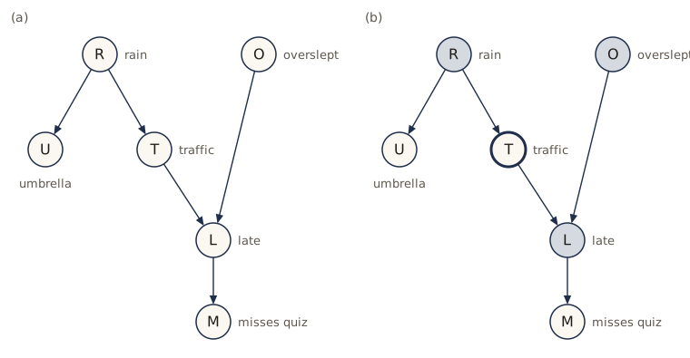
Reading the graph from panel (a), the joint distribution is
\[p(R, O, T, U, L, M) = p(R)\, p(O)\, p(T \mid R)\, p(U \mid R)\, p(L \mid T, O)\, p(M \mid L).\]We store each conditional distribution as a conditional probability table (CPT): an array with one axis per parent and a last axis for the variable itself. joint_table multiplies the tables together with np.einsum, lining up axes by variable, which is exactly the product above.
def bernoulli_table(p1):
    """CPT for a binary variable from P(x = 1), given as an array over the parent settings."""
    p1 = np.asarray(p1, dtype=float)
    return np.stack([1 - p1, p1], axis=-1)

commute_parents = {"R": (), "O": (), "T": ("R",), "U": ("R",), "L": ("T", "O"), "M": ("L",)}
commute_cpt = {
    "R": bernoulli_table(0.3),                        # p(R = 1)
    "O": bernoulli_table(0.2),                        # p(O = 1)
    "T": bernoulli_table([0.2, 0.7]),                 # p(T = 1 | R)
    "U": bernoulli_table([0.1, 0.8]),                 # p(U = 1 | R)
    "L": bernoulli_table([[0.05, 0.6], [0.4, 0.9]]),  # p(L = 1 | T, O), rows T, columns O
    "M": bernoulli_table([0.02, 0.7]),                # p(M = 1 | L)
}
commute_order = list(commute_parents)                 # R, O, T, U, L, M: a topological order

def joint_table(order, parents, cpt):
    """p(x) = prod_k p(x_k | pa_k) as an array with one axis per variable, axes in `order`."""
    idx = {v: i for i, v in enumerate(order)}
    operands = []
    for v in order:
        operands += [cpt[v], [idx[u] for u in parents[v]] + [idx[v]]]
    return np.einsum(*operands, list(range(len(order))))

def marginal(P, order, keep):
    """Marginal table over the variables in `keep` (axes in that order): sum out the rest."""
    idx = {v: i for i, v in enumerate(order)}
    return np.einsum(P, list(range(P.ndim)), [idx[v] for v in keep])

P = joint_table(commute_order, commute_parents, commute_cpt)
print("joint table shape", P.shape, " total probability", f"{P.sum():.6f}")
print("free numbers in a full joint table:", P.size - 1)
print("free numbers in the six CPTs:      ", sum(c[..., 1:].size for c in commute_cpt.values()))
p_RM = marginal(P, commute_order, ["R", "M"])
print(f"p(M = 1) = {p_RM[:, 1].sum():.4f}   "
      f"p(R = 1 | M = 1) = {p_RM[1, 1] / p_RM[:, 1].sum():.4f}")
joint table shape (2, 2, 2, 2, 2, 2)  total probability 1.000000
free numbers in a full joint table: 63
free numbers in the six CPTs:       12
p(M = 1) = 0.2097   p(R = 1 | M = 1) = 0.4158
A full table over six binary variables has 63 free numbers; the network needs 12. The saving comes entirely from the missing arrows. Once we have the joint table, any question is a sum: missing the quiz makes rain more likely, because rain is one of its indirect causes. Building the whole table, though, costs \(2^6\) entries here and \(K^M\) in general, so the rest of the module is about answering such questions without it.
Polynomial regression as a graph
The Bayesian regression model of module 03 is a Bayesian network too. Its random variables are the weight vector \(\mathbf{w}\) and the targets \(\mathbf{t} = (t_1, \dots, t_N)^{\mathrm{T}}\), and the joint distribution is a prior times \(N\) likelihood terms,
\[p(\mathbf{t}, \mathbf{w}) = p(\mathbf{w}) \prod_{n=1}^{N} p(t_n \mid \mathbf{w}).\]The graph has one arrow from \(\mathbf{w}\) to each \(t_n\). Drawing \(N\) nearly identical nodes gets tedious, so we use a shorthand: draw one representative node \(t_n\) and put a box around it labeled \(N\). The box is a plate, and it means “\(N\) copies of whatever is inside, with the same links”.
Three more conventions complete the picture. Quantities that are fixed rather than random, such as the inputs \(x_n\), the prior precision \(\alpha\), and the noise precision \(\beta\) (so the noise variance is \(\sigma^2 = 1/\beta\)), are drawn as small solid dots and called deterministic parameters. Variables whose values we observe, here the training targets, are drawn as shaded nodes; they are observed variables. Variables we never observe, like \(\mathbf{w}\), are latent (or hidden) variables. With all of it written out,
\[p(\mathbf{t}, \mathbf{w} \mid \mathbf{x}, \alpha, \beta) = p(\mathbf{w} \mid \alpha) \prod_{n=1}^{N} p(t_n \mid \mathbf{w}, x_n, \beta).\]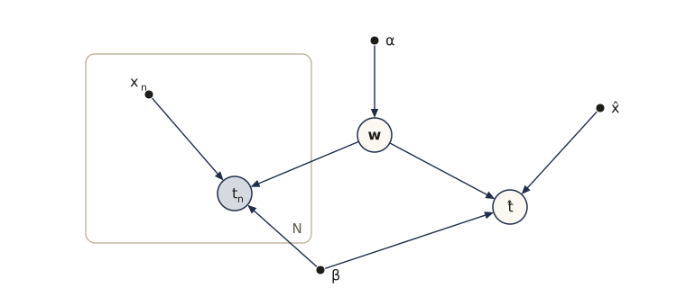
To predict at a new input \(\hat{x}\) we add a node \(\hat{t}\) with parents \(\mathbf{w}\), \(\hat{x}\), and \(\beta\). The posterior over the weights is proportional to the joint with the observed targets plugged in, and the predictive distribution integrates the weights out:
\[p(\mathbf{w} \mid \mathbf{t}) \propto p(\mathbf{w}) \prod_{n=1}^{N} p(t_n \mid \mathbf{w}), \qquad p(\hat{t} \mid \hat{x}, \mathbf{t}) = \int p(\hat{t} \mid \hat{x}, \mathbf{w})\, p(\mathbf{w} \mid \mathbf{t})\, \mathrm{d}\mathbf{w}.\]The graph gives the unnormalized posterior directly: it is the product of the factors. Here is a check with a straight-line model (\(M = 2\) weights), where we can evaluate that product on a fine grid of weight values, normalize it numerically, and compare the grid posterior mean with the closed form \(\mathbf{m}_N = \beta \mathbf{S}_N \mathbf{\Phi}^{\mathrm{T}} \mathbf{t}\), \(\mathbf{S}_N^{-1} = \alpha \mathbf{I} + \beta \mathbf{\Phi}^{\mathrm{T}} \mathbf{\Phi}\) from module 03.
alpha, beta = 2.0, 25.0
x_reg = rng.uniform(-1, 1, size=10)
t_reg = 0.3 - 0.8 * x_reg + rng.normal(0, 1 / np.sqrt(beta), size=10)
Phi = np.column_stack([np.ones_like(x_reg), x_reg])              # design matrix (N, M) = (10, 2)

# ln p(w) + sum_n ln p(t_n | w), up to constants, on a 401 x 401 grid of (w0, w1)
g0, g1 = np.meshgrid(np.linspace(-1, 1.5, 401), np.linspace(-2, 0.5, 401), indexing="ij")
Wgrid = np.column_stack([g0.ravel(), g1.ravel()])
log_joint = -0.5 * alpha * (Wgrid**2).sum(1) - 0.5 * beta * ((t_reg - Wgrid @ Phi.T)**2).sum(1)
post = np.exp(log_joint - logsumexp(log_joint))                   # normalized over the grid

S_N_inv = alpha * np.eye(2) + beta * Phi.T @ Phi
m_N = beta * np.linalg.solve(S_N_inv, Phi.T @ t_reg)
print("posterior mean, product of factors on a grid:", post @ Wgrid)
print("posterior mean, closed form:                 ", m_N)
posterior mean, product of factors on a grid: [ 0.3628 -0.786 ]
posterior mean, closed form:                  [ 0.3628 -0.786 ]
The two agree to the grid’s resolution. The graph also tells us something the algebra hid: once \(\mathbf{w}\) is known, the prediction \(\hat{t}\) has no other path to the training targets, so the data matter for prediction only through the posterior over \(\mathbf{w}\). We will make that kind of reasoning precise with d-separation below.
Generative models and ancestral sampling
A Bayesian network describes a way the data could have been produced: first draw the parentless variables, then each child given its parents. Turning this description into an algorithm gives ancestral sampling. Visit the nodes in topological order and draw each \(x_k\) from \(p(x_k \mid \mathrm{pa}_k)\) with its parents set to the values already drawn. The parents are always ready, because they come earlier in the order. After the last node we have one sample from the joint distribution. To sample from a marginal, such as \(p(T, M)\), sample everything and keep only the variables you want.
A model with this property, one that can produce synthetic data, is called a generative model. Typically the observed variables are the leaves of the graph and the latent variables sit above them. For example, an image of a handwritten digit could be modeled with a latent digit class, a latent stroke thickness, and a latent slant, all as parents of the observed pixels. Generating “fantasy” data from a fitted model is a good way to see what the model has actually learned. The regression graph above is not generative: the inputs \(x_n\) are fixed parameters with no distribution, so it cannot produce new inputs. We could make it generative by adding a distribution \(p(x)\).
def ancestral_sample(order, parents, cpt, n, rng):
    """n joint samples, visiting nodes parents-first; each draw uses the parents' sampled values."""
    s = {}
    for v in order:                                   # order must be topological
        probs = cpt[v][tuple(s[u] for u in parents[v])]           # (n, K_v), or (K_v,) at a root
        probs = np.broadcast_to(probs, (n, cpt[v].shape[-1]))
        u = rng.random(n)[:, None]
        draw = (u > np.cumsum(probs, axis=1)).sum(axis=1)         # inverse-CDF draw per row
        s[v] = np.minimum(draw, cpt[v].shape[-1] - 1)             # guard against round-off
    return s

S = ancestral_sample(commute_order, commute_parents, commute_cpt, 200_000, rng)
for v in commute_order:
    exact = marginal(P, commute_order, [v])[1]
    print(f"p({v} = 1): exact {exact:.4f}   from samples {S[v].mean():.4f}")
kept = S["M"] == 1
print(f"p(R = 1 | M = 1): exact {p_RM[1, 1] / p_RM[:, 1].sum():.4f}   "
      f"from the {kept.sum()} samples with M = 1: {S['R'][kept].mean():.4f}")
p(R = 1): exact 0.3000   from samples 0.2997
p(O = 1): exact 0.2000   from samples 0.1987
p(T = 1): exact 0.3500   from samples 0.3508
p(U = 1): exact 0.3100   from samples 0.3105
p(L = 1): exact 0.2790   from samples 0.2779
p(M = 1): exact 0.2097   from samples 0.2098
p(R = 1 | M = 1): exact 0.4158   from the 41965 samples with M = 1: 0.4149
Every sampled frequency is within a few thousandths of the exact value, as expected with 200,000 samples. The last line estimates a conditional probability by keeping only the samples that match the evidence. That works here, but it throws away most of the samples, and with rare evidence it throws away nearly all of them. Better sampling methods are the subject of module 11.
Discrete variables and parameter counts
Suppose each of \(M\) variables takes \(K\) values. A general table for their joint distribution has \(K^M - 1\) free numbers (the \(-1\) because the entries sum to one), which grows exponentially with \(M\). A Bayesian network replaces that table by one CPT per node: a node with \(K\) states whose parents have \(\prod_{u \in \mathrm{pa}} K_u\) joint settings needs \(K - 1\) numbers for each setting. Three graphs over \(M\) nodes mark out the range:
- Fully connected: \(K^M - 1\) numbers, the same as the full table, and it can represent anything.
- A chain \(x_1 \to x_2 \to \dots \to x_M\): \((K - 1) + (M - 1) K (K - 1)\) numbers, linear in \(M\).
- No links at all: \(M (K - 1)\) numbers, but only distributions in which all variables are independent.
Graphs in between trade flexibility against the number of parameters. Two more tools reduce the count further. Parameter sharing (or tying) uses one table for several nodes; in the chain, if all the transitions \(p(x_i \mid x_{i-1})\) share one \(K \times K\) table, the total drops to \(K^2 - 1\), independent of \(M\). And parameterized conditional distributions replace a table by a formula: a binary node \(y\) with \(M\) binary parents needs \(2^M\) numbers as a table, but only \(M + 1\) as a logistic regression on its parents (module 04),
\[p(y = 1 \mid x_1, \dots, x_M) = \sigma\Big(w_0 + \sum_{i=1}^{M} w_i x_i\Big) = \sigma(\mathbf{w}^{\mathrm{T}} \mathbf{x}),\]with \(x_0 = 1\) included in \(\mathbf{x}\). This restricts the kind of dependence on the parents, much as a diagonal covariance restricts a Gaussian.
def n_free_params(parents, states):
    """Free numbers in all the CPTs: (K_v - 1) for each joint setting of v's parents."""
    return sum((states[v] - 1) * int(np.prod([states[u] for u in parents[v]])) for v in parents)

def family(kind, M):
    nodes = [f"x{i}" for i in range(M)]
    if kind == "full":
        return {v: tuple(nodes[:i]) for i, v in enumerate(nodes)}
    if kind == "chain":
        return {v: (nodes[i - 1],) if i else () for i, v in enumerate(nodes)}
    return {v: () for v in nodes}                          # no links

print(" K   M    full table   fully connected      chain   shared chain   no links")
for K in (2, 3):
    for M in (5, 10):
        st = {f"x{i}": K for i in range(M)}
        full, chain, none = (n_free_params(family(k, M), st) for k in ("full", "chain", "none"))
        print(f"{K:2d} {M:3d} {K**M - 1:13d} {full:17d} {chain:10d} {K**2 - 1:14d} {none:10d}")
print("binary child with 10 binary parents: table", 2**10, "  logistic", 10 + 1)
 K   M    full table   fully connected      chain   shared chain   no links
 2   5            31                31          9              3          5
 2  10          1023              1023         19              3         10
 3   5           242               242         26              8         10
 3  10         59048             59048         56              8         20
binary child with 10 binary parents: table 1024   logistic 11
The fully connected count equals \(K^M - 1\) in every row, as it must, and the chain grows only linearly in \(M\).
We can also go Bayesian about the CPTs themselves. Put a Dirichlet prior (module 02) on each table’s parameters; in the graph, each discrete node gains an extra parent node \(\boldsymbol{\mu}_i\) holding its table. With tied parameters, a single node \(\boldsymbol{\mu}\) is a parent of all the nodes that share it.
Linear-Gaussian models
The other case where networks can be built up freely is when every node is a continuous variable whose conditional distribution is Gaussian with a mean that is linear in its parents:
\[p(x_i \mid \mathrm{pa}_i) = \mathcal{N}\Big(x_i \,\Big\vert\, \sum_{j \in \mathrm{pa}_i} w_{ij} x_j + b_i,\; v_i\Big).\]This is a linear-Gaussian model. Its log joint distribution is a sum of the logs of the conditionals,
\[\ln p(\mathbf{x}) = -\sum_{i=1}^{D} \frac{1}{2 v_i} \Big(x_i - \sum_{j \in \mathrm{pa}_i} w_{ij} x_j - b_i\Big)^2 + \text{const},\]which is a quadratic function of \(\mathbf{x} = (x_1, \dots, x_D)^{\mathrm{T}}\). A density whose logarithm is quadratic in \(\mathbf{x}\) (with a negative definite quadratic part, as here) is a multivariate Gaussian, so the whole joint distribution is Gaussian. All that remains is to find its mean and covariance.
The recursions. Write each node as its conditional mean plus independent noise: \(x_i = \sum_{j \in \mathrm{pa}_i} w_{ij} x_j + b_i + \sqrt{v_i}\, \epsilon_i\), with \(\epsilon_i\) standard normal and independent of everything earlier in the order. Taking expectations,
\[\mathbb{E}[x_i] = \sum_{j \in \mathrm{pa}_i} w_{ij}\, \mathbb{E}[x_j] + b_i .\]For the covariance of \(x_i\) with a node \(x_j\) that is not later in the order (\(i \le j\)), substitute the expansion of \(x_j\):
\[\begin{aligned} \operatorname{cov}[x_i, x_j] &= \mathbb{E}\Big[(x_i - \mathbb{E}[x_i]) \Big(\sum_{k \in \mathrm{pa}_j} w_{jk} (x_k - \mathbb{E}[x_k]) + \sqrt{v_j}\, \epsilon_j\Big)\Big] \\ &= \sum_{k \in \mathrm{pa}_j} w_{jk} \operatorname{cov}[x_i, x_k] + I_{ij}\, v_j . \end{aligned}\]The noise \(\epsilon_j\) is independent of \(x_i\) unless \(i = j\), which is where the \(I_{ij} v_j\) term comes from. Both recursions only look at earlier nodes, so we can fill in the mean vector and the covariance matrix one node at a time in topological order.
The same thing with matrices. Collect the weights in a matrix \(\mathbf{W}\) with entries \(w_{ij}\) (zero where \(j\) is not a parent of \(i\); in topological order it is strictly lower triangular), and let \(\mathbf{V} = \operatorname{diag}(v_1, \dots, v_D)\). Then \(\mathbf{x} = \mathbf{W}\mathbf{x} + \mathbf{b} + \mathbf{V}^{1/2} \boldsymbol{\epsilon}\), so \((\mathbf{I} - \mathbf{W}) \mathbf{x} = \mathbf{b} + \mathbf{V}^{1/2} \boldsymbol{\epsilon}\), and since \(\mathbf{I} - \mathbf{W}\) is unit lower triangular it is invertible:
\[\boldsymbol{\mu} = (\mathbf{I} - \mathbf{W})^{-1} \mathbf{b}, \qquad \boldsymbol{\Sigma} = (\mathbf{I} - \mathbf{W})^{-1} \mathbf{V} (\mathbf{I} - \mathbf{W})^{-\mathrm{T}}, \qquad \boldsymbol{\Lambda} = \boldsymbol{\Sigma}^{-1} = (\mathbf{I} - \mathbf{W})^{\mathrm{T}} \mathbf{V}^{-1} (\mathbf{I} - \mathbf{W}).\]Let us check all three routes on a four-node “diamond”: \(x_1 \to x_2\), \(x_1 \to x_3\), and \(x_2, x_3 \to x_4\).
lg_parents = {0: [], 1: [0], 2: [0], 3: [1, 2]}         # nodes 0..3 = x1..x4, topological order
W_lg = np.zeros((4, 4))
W_lg[1, 0], W_lg[2, 0], W_lg[3, 1], W_lg[3, 2] = 0.8, -0.5, 1.2, 0.7   # W[i, j] = w_ij
b_lg = np.array([1.0, 0.0, 2.0, -1.0])
v_lg = np.array([1.0, 0.5, 0.3, 0.2])

def lg_moments(parents, W, b, v):
    """Mean and covariance of a linear-Gaussian network, node by node (the two recursions)."""
    D = len(b)
    mu, Sigma = np.zeros(D), np.zeros((D, D))
    for j in range(D):
        mu[j] = sum(W[j, k] * mu[k] for k in parents[j]) + b[j]
        for i in range(j + 1):                          # cov[x_i, x_j] for i < j, then i = j
            Sigma[i, j] = sum(W[j, k] * Sigma[i, k] for k in parents[j]) + (v[j] if i == j else 0.0)
            Sigma[j, i] = Sigma[i, j]
    return mu, Sigma

mu_rec, Sigma_rec = lg_moments(lg_parents, W_lg, b_lg, v_lg)
A = np.eye(4) - W_lg
L_half = np.linalg.solve(A, np.diag(np.sqrt(v_lg)))    # (I - W)^{-1} V^{1/2}
print("mean:", mu_rec, "  matrix form agrees:", np.allclose(mu_rec, np.linalg.solve(A, b_lg)))
print("covariance:\n", Sigma_rec)
print("matrix form agrees:", np.allclose(Sigma_rec, L_half @ L_half.T))

# ancestral sampling of the same network
n = 200_000
X = np.zeros((n, 4))
for j in range(4):
    pa = lg_parents[j]
    X[:, j] = X[:, pa] @ W_lg[j, pa] + b_lg[j] + np.sqrt(v_lg[j]) * rng.standard_normal(n)
print(f"sampling: largest error in the mean {np.abs(X.mean(0) - mu_rec).max():.4f}, "
      f"in the covariance {np.abs(np.cov(X.T) - Sigma_rec).max():.4f}")
print("precision matrix:\n", A.T @ np.diag(1 / v_lg) @ A)
mean: [1.   0.8  1.5  1.01]   matrix form agrees: True
covariance:
 [[ 1.      0.8    -0.5     0.61  ]
 [ 0.8     1.14   -0.4     1.088 ]
 [-0.5    -0.4     0.55   -0.095 ]
 [ 0.61    1.088  -0.095   1.4391]]
matrix form agrees: True
sampling: largest error in the mean 0.0054, in the covariance 0.0050
precision matrix:
 [[ 3.1133 -1.6     1.6667  0.    ]
 [-1.6     9.2     4.2    -6.    ]
 [ 1.6667  4.2     5.7833 -3.5   ]
 [ 0.     -6.     -3.5     5.    ]]
The recursion, the matrix formula, and 200,000 ancestral samples all agree. Look at the precision matrix: its entry for the pair \((x_1, x_4)\) is exactly zero, although the covariance between them is not. For a Gaussian, a zero in the precision matrix means the two variables are conditionally independent given all the others (module 02). The graph predicts this: \(x_1\) influences \(x_4\) only through \(x_2\) and \(x_3\). The pair \((x_2, x_3)\), on the other hand, has a nonzero precision entry even though there is no arrow between them, because they share the child \(x_4\). Both facts will make sense after the next two sections.
The two extremes behave as you would expect. With no links, \(\boldsymbol{\Sigma} = \mathbf{V}\) is diagonal and the model has \(2D\) parameters. With every possible link, \(\mathbf{W}\) has \(D(D-1)/2\) free entries below the diagonal, and together with the \(D\) variances that is \(D(D+1)/2\), exactly the number of free entries of a general covariance matrix. The same construction works when each node is a Gaussian vector and the weights are matrices, and it is the backbone of probabilistic PCA and factor analysis (module 12) and of the linear dynamical systems of module 13.
You have already met a two-node linear-Gaussian network: in module 02, a Gaussian prior on the mean \(\mu\) of a Gaussian variable \(x\) is the graph \(\mu \to x\), and the joint of \(\mu\) and \(x\) is Gaussian. If the prior’s own mean is uncertain we can give it a Gaussian prior too (a hyperprior), adding a node above \(\mu\). Stacking priors like this gives a hierarchical Bayesian model.
Conditional independence
Definition. Variables \(a\) and \(b\) are conditionally independent given \(c\) if \(p(a \mid b, c) = p(a \mid c)\) for every value of \(b\) and every value of \(c\) with \(p(b, c) > 0\). Equivalently, \(p(a, b \mid c) = p(a \mid c)\, p(b \mid c)\): once \(c\) is known, the joint of \(a\) and \(b\) factorizes. We write \(a \perp\!\!\!\perp b \mid c\), and \(a \perp\!\!\!\perp b \mid \emptyset\) (or \(a \perp\!\!\!\perp b\)) for plain independence. The same definition applies to disjoint sets of variables \(A\), \(B\), \(C\).
The condition must hold for all values of \(c\), not just some. Conditional independence is what makes a model cheap to store and fast to compute with, and the remarkable fact about graphical models is that we can read these properties off the graph, without touching the numbers.
To check such claims numerically we need a test on a joint table. Multiplying the definition through by \(p(c)^2\) gives a form with no division, which also behaves sensibly when \(p(c) = 0\):
\[p(a, b, c)\, p(c) = p(a, c)\, p(b, c) \quad \text{for all } a, b, c.\]cond_indep_gap returns the largest violation of this equation. It is zero (up to round-off) exactly when \(A \perp\!\!\!\perp B \mid C\) holds.
def cond_indep_gap(P, A, B, C=()):
    """max |p(a,b,c) p(c) - p(a,c) p(b,c)| over all values; 0 means A and B are independent given C.
    A, B, C: collections of axis numbers of the joint table P."""
    def m(keep):
        return P.sum(axis=tuple(i for i in range(P.ndim) if i not in keep), keepdims=True)
    A, B, C = set(A), set(B), set(C)
    return np.abs(m(A | B | C) * m(C) - m(A | C) * m(B | C)).max()
Three basic graphs
Everything about conditional independence in directed graphs follows from three graphs on three nodes, which differ in how the two arrows meet at \(c\).
Tail-to-tail, \(a \leftarrow c \rightarrow b\). The joint is \(p(a, b, c) = p(a \mid c)\, p(b \mid c)\, p(c)\). Summing out \(c\) gives \(p(a, b) = \sum_c p(a \mid c)\, p(b \mid c)\, p(c)\), which is a mixture and usually not a product \(p(a) p(b)\): \(a\) and \(b\) are dependent because they share a cause. Conditioning on \(c\) instead gives \(p(a, b \mid c) = p(a, b, c) / p(c)\), which is \(p(a \mid c)\, p(b \mid c)\), so \(a \perp\!\!\!\perp b \mid c\). We say \(c\) is a tail-to-tail node on the path from \(a\) to \(b\) (it touches the tails of both arrows). An unobserved tail-to-tail node leaves the path open; an observed one blocks it.
Head-to-tail, \(a \rightarrow c \rightarrow b\). Now \(p(a, b, c) = p(a)\, p(c \mid a)\, p(b \mid c)\), and summing out \(c\) gives \(p(a) \sum_c p(c \mid a)\, p(b \mid c)\), which is \(p(a)\, p(b \mid a)\) and again need not equal \(p(a) p(b)\): influence flows along the chain. Given \(c\),
\[p(a, b \mid c) = \frac{p(a)\, p(c \mid a)\, p(b \mid c)}{p(c)} = p(a \mid c)\, p(b \mid c)\]by Bayes’ theorem, so \(a \perp\!\!\!\perp b \mid c\). A head-to-tail node behaves like a tail-to-tail one: open when unobserved, blocking when observed.
Head-to-head, \(a \rightarrow c \leftarrow b\). Here \(p(a, b, c) = p(a)\, p(b)\, p(c \mid a, b)\). Summing out \(c\) gives \(p(a, b) = p(a)\, p(b)\) at once, so \(a \perp\!\!\!\perp b\): two independent causes of a common effect are independent. But given \(c\),
\[p(a, b \mid c) = \frac{p(a)\, p(b)\, p(c \mid a, b)}{p(c)},\]and for most choices of \(p(c \mid a, b)\) this is not a product of a function of \(a\) and a function of \(b\). Observing a head-to-head node opens the path, the opposite of the other two cases. One more subtlety: the path also opens if any descendant of \(c\) is observed (a node reachable from \(c\) by following arrows), because a descendant carries information about \(c\).
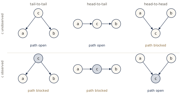
Now the numerical check. For each graph we draw random CPTs (each row a random draw from a flat Dirichlet), build the joint table with axes \((a, b, c)\), and measure both independence gaps.
graphs3 = {
    "tail-to-tail  a <- c -> b": {"a": ("c",), "b": ("c",), "c": ()},
    "head-to-tail  a -> c -> b": {"a": (), "b": ("c",), "c": ("a",)},
    "head-to-head  a -> c <- b": {"a": (), "b": (), "c": ("a", "b")},
}
print(f"{'graph':27s} {'gap for a, b':>13s} {'gap for a, b given c':>22s}")
for name, pa in graphs3.items():
    cpt = {v: rng.dirichlet(np.ones(2), size=(2,) * len(pa[v])) for v in pa}
    P3 = joint_table(["a", "b", "c"], pa, cpt)
    gap0, gap_c = cond_indep_gap(P3, [0], [1]), cond_indep_gap(P3, [0], [1], [2])
    print(f"{name:27s} {gap0:13.2e} {gap_c:22.2e}")
graph                        gap for a, b   gap for a, b given c
tail-to-tail  a <- c -> b        3.65e-03               1.39e-17
head-to-tail  a -> c -> b        1.63e-02               1.39e-17
head-to-head  a -> c <- b        5.55e-17               2.72e-02
A gap near \(10^{-17}\) is round-off; a gap of \(10^{-3}\) or more is a real dependence. The pattern matches the derivations: only the head-to-head graph has \(a\) and \(b\) independent before we observe \(c\), and only it loses the independence after.
Explaining away
The head-to-head case deserves a story, because it is the one that surprises people. You submit a programming assignment and the autograder reports a failure. Two things could cause that: a bug in your code (\(B\)), or a misconfigured autograder (\(S\), for server). The two causes are independent before anything is observed: your bug does not care about the server. Here are the numbers:
| \(S = 0\) | \(S = 1\) | |
|---|---|---|
| \(p(F = 1 \mid B = 0, S)\) | 0.02 | 0.95 |
| \(p(F = 1 \mid B = 1, S)\) | 0.90 | 0.99 |
with priors \(p(B = 1) = 0.25\) and \(p(S = 1) = 0.05\).
ag_parents = {"B": (), "S": (), "F": ("B", "S")}
ag_cpt = {"B": bernoulli_table(0.25), "S": bernoulli_table(0.05),
          "F": bernoulli_table([[0.02, 0.95], [0.90, 0.99]])}      # rows B, columns S
PF = joint_table(["B", "S", "F"], ag_parents, ag_cpt)               # axes (B, S, F)

print(f"p(bug)                          = {PF[1].sum():.3f}")
print(f"p(bug | fail)                   = {PF[1, :, 1].sum() / PF[:, :, 1].sum():.3f}")
print(f"p(bug | fail, server broken)    = {PF[1, 1, 1] / PF[:, 1, 1].sum():.3f}")
print(f"p(bug | fail, server fine)      = {PF[1, 0, 1] / PF[:, 0, 1].sum():.3f}")
print(f"gap for B, S: {cond_indep_gap(PF, [0], [1]):.1e}   "
      f"given F: {cond_indep_gap(PF, [0], [1], [2]):.1e}")
p(bug)                          = 0.250
p(bug | fail)                   = 0.819
p(bug | fail, server broken)    = 0.258
p(bug | fail, server fine)      = 0.938
gap for B, S: 1.1e-16   given F: 7.4e-03
The failure makes a bug much more likely, up from a quarter to over four fifths. Then a classmate posts that the autograder is broken for everyone. Nothing about your code has changed, yet the probability that it has a bug falls almost back to the prior: the broken server explains away the failure. Hearing instead that the server is fine pushes the bug probability higher still. So \(B\) and \(S\), independent a priori, became dependent once we observed their common effect. The posterior with both observations stays slightly above the prior 0.25 because even a broken server fails a buggy submission a little more reliably.
Watch out. “Conditioning can only remove dependence” is false. Observing a common effect, or anything downstream of it, creates dependence between its causes. This is behind many real-world statistical traps, such as selecting a sample on an outcome and then finding spurious correlations among the outcome’s causes.
D-separation
For larger graphs we look at every path between two sets of nodes, ignoring the arrow directions, and ask whether something along it blocks it.
Definition. Let \(A\), \(B\), \(C\) be disjoint sets of nodes in a DAG. Then \(A\) is d-separated from \(B\) by \(C\) if every path (a sequence of linked nodes, arrows in either direction) from a node in \(A\) to a node in \(B\) is blocked by \(C\), meaning that it passes through a node \(v\) where either
- \(v\) is a head-to-tail or tail-to-tail node on the path, and \(v\) is in \(C\); or
- \(v\) is a head-to-head node on the path, and neither \(v\) nor any of its descendants is in \(C\).
D-separation guarantees that \(A \perp\!\!\!\perp B \mid C\) holds for every distribution that factorizes according to the graph.
Try it on the commute network. \(T\) and \(U\) are connected only through \(R\), tail-to-tail, so \(T \perp\!\!\!\perp U \mid R\). \(R\) and \(O\) meet only head-to-head at \(L\), so \(R \perp\!\!\!\perp O\); but observing \(L\), or its descendant \(M\), opens that path. And \(R\) reaches \(M\) only through \(L\), where the arrows meet head-to-tail, so \(R \perp\!\!\!\perp M \mid L\).
Checking every path by hand gets out of control, since the number of paths can grow exponentially. There is a linear-time algorithm instead, often described as a ball bouncing through the graph (the “Bayes ball”). We search over pairs (node, direction of arrival): arriving “up” means we came from a child, arriving “down” means we came from a parent. The three rules become:
- Arriving up at an unobserved node (so the node is a tail on the incoming link): the path can continue to any parent (head-to-tail) or any child (tail-to-tail).
- Arriving down at an unobserved node: the path can continue to its children (head-to-tail). It cannot turn back up, because that would make the node head-to-head.
- Arriving down at a node that is in \(C\) or has a descendant in \(C\): the path can turn up to the node’s parents (an open head-to-head node).
A first pass collects the nodes that are in \(C\) or have a descendant in \(C\), which is the same as the ancestors of \(C\) together with \(C\) itself.
def d_separated(parents, X, Y, Z):
    """True if X and Y are d-separated by Z in the DAG given by `parents` (reachability search)."""
    children = {v: [] for v in parents}
    for v, pa in parents.items():
        for u in pa:
            children[u].append(v)
    Z = set(Z)
    opens_v = set()                                  # Z and all ancestors of Z
    stack = list(Z)
    while stack:
        v = stack.pop()
        if v not in opens_v:
            opens_v.add(v)
            stack.extend(parents[v])
    reached, visited = set(), set()
    stack = [(x, "up") for x in X]                   # "up" = arrived from a child
    while stack:
        v, d = stack.pop()
        if (v, d) in visited:
            continue
        visited.add((v, d))
        if v not in Z:
            reached.add(v)
        if d == "up" and v not in Z:
            stack += [(u, "up") for u in parents[v]]      # head-to-tail, going up
            stack += [(c, "down") for c in children[v]]   # tail-to-tail
        elif d == "down":
            if v not in Z:
                stack += [(c, "down") for c in children[v]]   # head-to-tail, going down
            if v in opens_v:
                stack += [(u, "up") for u in parents[v]]      # open head-to-head node
    return not (reached & set(Y))

queries = [("T", "U", []), ("T", "U", ["R"]), ("R", "O", []), ("R", "O", ["L"]),
           ("R", "O", ["M"]), ("R", "M", []), ("R", "M", ["L"]), ("U", "M", ["T", "O"])]
cidx = {v: i for i, v in enumerate(commute_order)}
for a, b, Z in queries:
    sep = d_separated(commute_parents, [a], [b], Z)
    gap = cond_indep_gap(P, [cidx[a]], [cidx[b]], [cidx[z] for z in Z])
    given = "{" + ",".join(Z) + "}"
    print(f"{a}, {b} given {given:7s} d-separated {str(sep):5s}  gap {gap:.1e}")
T, U given {}      d-separated False  gap 7.4e-02
T, U given {R}     d-separated True   gap 5.6e-17
R, O given {}      d-separated True   gap 2.8e-17
R, O given {L}     d-separated False  gap 3.3e-03
R, O given {M}     d-separated False  gap 1.5e-03
R, M given {}      d-separated False  gap 2.4e-02
R, M given {L}     d-separated True   gap 5.6e-17
U, M given {T,O}   d-separated True   gap 2.8e-17
Each “True” comes with a gap at round-off level and each “False” with a clearly nonzero gap. The last query is worth tracing: the path \(U \leftarrow R \rightarrow T \rightarrow L \rightarrow M\) is blocked at \(T\), which is observed and head-to-tail on it.
A few spot checks are not a proof, so let us compare the algorithm with brute force on every pair of variables and every conditioning set drawn from the remaining variables, first on the commute network and then on twenty random networks with seven nodes, random links, two or three states per node, and random CPTs.
def random_network(n, p_edge, rng, max_parents=3):
    """Random DAG on v0..v{n-1} (numbering = topological order) with random states and CPTs."""
    order = [f"v{i}" for i in range(n)]
    parents = {v: tuple([u for u in order[:i] if rng.random() < p_edge][:max_parents])
               for i, v in enumerate(order)}
    states = {v: int(rng.integers(2, 4)) for v in order}
    cpt = {v: rng.dirichlet(np.ones(states[v]), size=tuple(states[u] for u in parents[v]))
           for v in order}
    return order, parents, cpt

def compare_dsep(order, parents, P):
    """d-separation versus the brute-force gap for all pairs and all conditioning sets."""
    idx = {v: i for i, v in enumerate(order)}
    n_q = n_sep = mismatches = 0
    worst_sep, closest_dep = 0.0, np.inf
    for a, b in combinations(order, 2):
        rest = [v for v in order if v not in (a, b)]
        for r in range(len(rest) + 1):
            for Z in combinations(rest, r):
                sep = d_separated(parents, [a], [b], Z)
                gap = cond_indep_gap(P, [idx[a]], [idx[b]], [idx[z] for z in Z])
                n_q += 1
                n_sep += sep
                mismatches += sep != (gap < 1e-12)
                if sep:
                    worst_sep = max(worst_sep, gap)
                else:
                    closest_dep = min(closest_dep, gap)
    return n_q, n_sep, mismatches, worst_sep, closest_dep

q, s, bad, ws, cd = compare_dsep(commute_order, commute_parents, P)
print(f"commute network: {q} queries, {s} d-separated, {bad} disagreements")
totals = np.zeros(3, dtype=int)
worst, closest = 0.0, np.inf
for _ in range(20):
    order, pa, cpt = random_network(7, 0.35, rng)
    q, s, bad, ws, cd = compare_dsep(order, pa, joint_table(order, pa, cpt))
    totals += (q, s, bad)
    worst, closest = max(worst, ws), min(closest, cd)
print(f"20 random networks: {totals[0]} queries, {totals[1]} d-separated, "
      f"{totals[2]} disagreements")
print(f"largest gap when d-separated {worst:.1e};  smallest gap when not {closest:.1e}")
commute network: 240 queries, 97 d-separated, 0 disagreements
20 random networks: 13440 queries, 6008 d-separated, 0 disagreements
largest gap when d-separated 7.8e-16;  smallest gap when not 6.0e-07
The algorithm and brute force agree on every one of the queries, and there is a wide margin between round-off and the weakest real dependence. Notice what the test relies on. D-separation guarantees independence. The converse is not guaranteed: when a path is open, the graph permits dependence, but particular numbers in the CPTs could cancel it. With randomly drawn CPTs such cancellations have probability zero, which is why brute force finds a dependence every time the algorithm says “not d-separated”.
Deterministic parameters, such as \(\alpha\) and \(\beta\) in the regression graph, behave like observed nodes in d-separation. They have no parents, so every path through them is tail-to-tail at an observed node and blocked; they never matter.
Three applications of d-separation
Independent and identically distributed data. Suppose we infer the mean \(\mu\) of a Gaussian from observations \(x_1, \dots, x_N\). The graph is \(\mu \to x_n\) inside a plate. Every path between two observations goes through \(\mu\), tail-to-tail, so given \(\mu\) the observations are independent and \(p(\mathcal{D} \mid \mu) = \prod_n p(x_n \mid \mu)\). But \(\mu\) is latent, and with \(\mu\) summed out the path is open: the observations are not independent under the marginal \(p(\mathcal{D})\). Our linear-Gaussian code makes this concrete. With prior \(\mu \sim \mathcal{N}(0, 4)\) and \(x_n \mid \mu \sim \mathcal{N}(\mu, 1)\) for three observations:
iid_parents = {0: [], 1: [0], 2: [0], 3: [0]}          # node 0 is mu, nodes 1-3 are x1..x3
W_iid = np.zeros((4, 4))
W_iid[1:, 0] = 1.0
_, Sig_iid = lg_moments(iid_parents, W_iid, np.zeros(4), np.array([4.0, 1.0, 1.0, 1.0]))
print("cov of (x1, x2, x3) with mu unknown:\n", Sig_iid[1:, 1:])
# condition on mu with the Gaussian conditioning formula of module 02
cond = Sig_iid[1:, 1:] - np.outer(Sig_iid[1:, 0], Sig_iid[0, 1:]) / Sig_iid[0, 0]
print("cov of (x1, x2, x3) given mu:\n", cond)
cov of (x1, x2, x3) with mu unknown:
 [[5. 4. 4.]
 [4. 5. 4.]
 [4. 4. 5.]]
cov of (x1, x2, x3) given mu:
 [[1. 0. 0.]
 [0. 1. 0.]
 [0. 0. 1.]]
Before we know \(\mu\), each pair of observations has covariance 4, the prior variance of \(\mu\): seeing a large \(x_1\) suggests a large \(\mu\) and hence a large \(x_2\). Given \(\mu\), the covariance is the identity. Learning from data works precisely because the observations are dependent through the unknown parameter.
Prediction depends on the data only through the posterior. In the regression graph, every path from \(\hat{t}\) to a training target \(t_n\) goes through \(\mathbf{w}\), tail-to-tail. So \(\hat{t} \perp\!\!\!\perp t_n \mid \mathbf{w}\): we can compute the posterior over \(\mathbf{w}\), throw the training set away, and still make the same predictions.
Naive Bayes. A classifier with a class variable \(z\) (1-of-\(K\) coded) and features \(x_1, \dots, x_D\) can assume that the features are independent given the class. The graph is \(z \to x_i\) for each \(i\), and \(z\) is tail-to-tail on every path between features: \(x_i \perp\!\!\!\perp x_j \mid z\). This is the naive Bayes model. It is fit by maximum likelihood one class at a time, and with Gaussian features it gives each class a diagonal covariance. Because \(z\) is unobserved at test time, the features are still dependent under the marginal \(p(\mathbf{x})\), which is a mixture of the class densities. The independence assumption is usually wrong, yet the classifier often works well: it needs few parameters in high dimensions, it mixes discrete and continuous features easily, and a decision boundary can be accurate even when the densities behind it are not.
Graphs as filters
There are two ways to say what distributions a DAG describes. The first uses factorization: pass every possible distribution over the variables through a filter that lets \(p(\mathbf{x})\) through only if it can be written as \(\prod_k p(x_k \mid \mathrm{pa}_k)\). Call the survivors \(\mathcal{DF}\), for directed factorization. The second uses independence: list every statement \(A \perp\!\!\!\perp B \mid C\) that d-separation reads off the graph, and let through only the distributions that satisfy all of them. The d-separation theorem says the two filters pass exactly the same set.
This is a statement about a family of distributions, not about one. It holds whether the variables are discrete, continuous, or mixed. A fully connected DAG implies no independences and passes every distribution; a DAG with no links passes only fully factorized distributions. Any graph also passes distributions with extra independences that the graph does not show; for instance, a fully factorized distribution passes every filter. That is why the random-network check above needed random CPTs.
The Markov blanket
What is the smallest set of variables that makes a node \(x_i\) independent of everything else? Write the conditional of \(x_i\) given all the other variables using the factorization:
\[p(x_i \mid \mathbf{x}_{\setminus i}) = \frac{\prod_k p(x_k \mid \mathrm{pa}_k)}{\sum_{x_i} \prod_k p(x_k \mid \mathrm{pa}_k)}.\](For continuous variables the sum is an integral.) Every factor that does not contain \(x_i\) comes out of the sum and cancels. What remains is \(p(x_i \mid \mathrm{pa}_i)\) and the factors \(p(x_k \mid \mathrm{pa}_k)\) of the children of \(x_i\), which also involve the children’s other parents. So the conditional involves only three groups of variables: the node’s parents, its children, and its co-parents (the children’s other parents). This set is the Markov blanket of \(x_i\). The co-parents are needed because of explaining away: observing a child opens the path to its other parents.
def markov_blanket(parents, v):
    children = [c for c, pa in parents.items() if v in pa]
    co_parents = {u for c in children for u in parents[c]} - {v}
    return set(parents[v]) | set(children) | co_parents

def conditional_given(P, i, keep):
    """p(x_i | x_keep), broadcast against the full table P."""
    m = P.sum(axis=tuple(j for j in range(P.ndim) if j not in keep and j != i), keepdims=True)
    return m / m.sum(axis=i, keepdims=True)

iT = cidx["T"]
mb = markov_blanket(commute_parents, "T")
everything_else = [j for j in range(P.ndim) if j != iT]
full = conditional_given(P, iT, everything_else)
print("Markov blanket of T:", sorted(mb))
print(f"p(T | all others) vs p(T | blanket):         max difference "
      f"{np.abs(full - conditional_given(P, iT, [cidx[v] for v in mb])).max():.1e}")
print(f"p(T | all others) vs p(T | parent and child): max difference "
      f"{np.abs(full - conditional_given(P, iT, [cidx['R'], cidx['L']])).max():.1e}")
Markov blanket of T: ['L', 'O', 'R']
p(T | all others) vs p(T | blanket):         max difference 1.1e-16
p(T | all others) vs p(T | parent and child): max difference 2.3e-01
Conditioning on the blanket \(\{R, L, O\}\) reproduces the full conditional exactly; dropping the co-parent \(O\) changes it. Panel (b) of the first figure shows this blanket. The Markov blanket is what Gibbs sampling (module 11) needs: to resample one variable, you look only at its blanket.
Markov random fields
Directed graphs have one awkward feature: the head-to-head rule makes independence depend on arrow directions in a subtle way. An undirected graph removes the arrows, and with them the subtlety.
A Markov random field (also Markov network or undirected graphical model) is an undirected graph over the variables together with a distribution that factorizes over the graph’s cliques, as described below. Its independence properties are read off by plain graph separation.
Conditional independence by graph separation
In an undirected graph, \(A \perp\!\!\!\perp B \mid C\) is implied when every path from a node in \(A\) to a node in \(B\) goes through some node of \(C\). Equivalently, delete the nodes of \(C\) (and their links) and check that no path is left from \(A\) to \(B\). There is no explaining away and no special case. In particular the Markov blanket of a node is simply its set of neighbors.
For the next few code cells we use the undirected graph on \(x_1, \dots, x_6\) with links \(x_1x_2\), \(x_1x_3\), \(x_2x_3\), \(x_3x_4\), \(x_3x_5\), \(x_4x_5\), \(x_5x_6\): two triangles joined at \(x_3\) and a tail at \(x_5\). It is drawn in panel (b) of the figure in the section on directed graphs below, where we will see where it comes from.
def undirected(edges):
    adj = {}
    for u, v in edges:
        adj.setdefault(u, set()).add(v)
        adj.setdefault(v, set()).add(u)
    return adj

def separated(adj, A, B, C):
    """True if every path from A to B goes through C: search from A with C deleted."""
    C = set(C)
    seen, stack = set(A), list(A)
    while stack:
        for v in adj[stack.pop()]:
            if v not in seen and v not in C:
                seen.add(v)
                stack.append(v)
    return not (seen & set(B))

adj_u = undirected([("x1", "x2"), ("x1", "x3"), ("x2", "x3"), ("x3", "x4"),
                    ("x3", "x5"), ("x4", "x5"), ("x5", "x6")])
print(separated(adj_u, ["x1"], ["x6"], ["x3"]), separated(adj_u, ["x1"], ["x6"], ["x4"]),
      separated(adj_u, ["x4"], ["x6"], ["x5"]), separated(adj_u, ["x2"], ["x4"], []))
True False True False
Given \(x_3\), the first triangle is cut off from the rest, so \(x_1\) and \(x_6\) are separated; given \(x_4\) instead, the path through \(x_3\) and \(x_5\) remains. Likewise \(x_5\) separates the tail \(x_6\) from everything else, while \(x_2\) and \(x_4\) are linked through \(x_3\) when nothing is observed.
Factorization over cliques
What factorization matches graph separation? If \(x_i\) and \(x_j\) are not linked, every path between them passes through other nodes, so they must be independent given all the other variables:
\[p(x_i, x_j \mid \mathbf{x}_{\setminus \{i,j\}}) = p(x_i \mid \mathbf{x}_{\setminus \{i,j\}})\, p(x_j \mid \mathbf{x}_{\setminus \{i,j\}}).\]For that to hold in general, \(x_i\) and \(x_j\) must never appear together in one factor. So the factors should live on sets of nodes that are all linked to each other.
\[p(\mathbf{x}) = \frac{1}{Z} \prod_{C} \psi_C(\mathbf{x}_C), \qquad Z = \sum_{\mathbf{x}} \prod_{C} \psi_C(\mathbf{x}_C).\]Definition. A clique is a set of nodes in which every pair is linked. A maximal clique is a clique that cannot be enlarged by adding another node. A Markov random field assigns a nonnegative potential function \(\psi_C(\mathbf{x}_C)\) to each maximal clique \(C\) and defines the joint distribution as their normalized product, displayed below.
The normalizer \(Z\) is called the partition function. Factors on smaller cliques add nothing, because they can be multiplied into a maximal clique that contains them. Unlike the CPTs of a Bayesian network, potentials have no probabilistic meaning of their own: they are not marginals or conditionals, and they need not sum to anything. The price of that freedom is the partition function, which in general is a sum over all \(K^M\) joint states. We need \(Z\) to learn the potentials’ parameters, since it depends on them. We do not need it for conditionals, where it cancels, or for marginals of a few variables, which we can normalize at the end.
Hammersley–Clifford. Restrict to potentials that are strictly positive. Let \(\mathcal{UI}\) be the distributions that satisfy all separation statements of the graph and \(\mathcal{UF}\) the distributions that factorize over its maximal cliques. The Hammersley–Clifford theorem says \(\mathcal{UI} = \mathcal{UF}\): the undirected analogue of the d-separation theorem. Strictly positive potentials can be written as \(\psi_C(\mathbf{x}_C) = \exp\{-E(\mathbf{x}_C)\}\) with an energy function \(E\), and the joint \(p(\mathbf{x}) \propto \exp\{-\sum_C E(\mathbf{x}_C)\}\) is a Boltzmann distribution: low total energy means high probability. Choosing potentials becomes choosing which local configurations to reward.
Here is our six-node graph with random positive potentials. We find the maximal cliques with the Bron–Kerbosch recursion (grow a clique \(R\) from candidates \(P\), skipping nodes \(X\) already handled), compute \(Z\) by brute force, and then repeat the brute-force independence comparison, this time against graph separation.
def maximal_cliques(adj):
    """All maximal cliques (Bron-Kerbosch without pivoting); fine for small graphs."""
    found = []
    def extend(R, P, X):
        if not P and not X:
            found.append(sorted(R))
        for v in sorted(P):
            extend(R | {v}, P & adj[v], X & adj[v])
            P, X = P - {v}, X | {v}
    extend(set(), set(adj), set())
    return sorted(found)

mrf_order = ["x1", "x2", "x3", "x4", "x5", "x6"]
midx = {v: i for i, v in enumerate(mrf_order)}
cliques = maximal_cliques(adj_u)
psi = {tuple(C): np.exp(rng.normal(size=(2,) * len(C))) for C in cliques}   # psi = exp(-E)
ops = []
for C, table in psi.items():
    ops += [table, [midx[v] for v in C]]
unnorm = np.einsum(*ops, list(range(6)))
Z = unnorm.sum()
Pm = unnorm / Z
print("maximal cliques:", cliques, f"  Z = {Z:.4f}")

bad, n_q, worst, closest = 0, 0, 0.0, np.inf
for a, b in combinations(mrf_order, 2):
    rest = [v for v in mrf_order if v not in (a, b)]
    for r in range(len(rest) + 1):
        for C in combinations(rest, r):
            sep = separated(adj_u, [a], [b], C)
            gap = cond_indep_gap(Pm, [midx[a]], [midx[b]], [midx[c] for c in C])
            n_q += 1
            bad += sep != (gap < 1e-12)
            if sep:
                worst = max(worst, gap)
            else:
                closest = min(closest, gap)
print(f"{n_q} queries, {bad} disagreements; largest gap when separated {worst:.1e}, "
      f"smallest when not {closest:.1e}")

p56 = marginal(Pm, mrf_order, ["x5", "x6"])
psi56 = psi[("x5", "x6")]
print("p(x5, x6):\n", p56, "\npsi(x5, x6) normalized:\n", psi56 / psi56.sum())
maximal cliques: [['x1', 'x2', 'x3'], ['x3', 'x4', 'x5'], ['x5', 'x6']]   Z = 396.7687
240 queries, 0 disagreements; largest gap when separated 5.6e-17, smallest when not 2.5e-04
p(x5, x6):
 [[0.2145 0.3005]
 [0.4502 0.0347]]
psi(x5, x6) normalized:
 [[0.2245 0.3146]
 [0.4279 0.033 ]]
Graph separation and brute force agree on all 240 queries. The last lines show that a potential is not a marginal: the potential on the clique \(\{x_5, x_6\}\), normalized, is close to the actual \(p(x_5, x_6)\) but not equal to it, because the other clique that contains \(x_5\) also pulls on it.
Image de-noising with an Ising model
Here is a Markov random field doing real work. We have a binary image with pixels \(x_i \in \{-1, +1\}\), \(i = 1, \dots, D\), which we cannot see. We observe a noisy copy \(y_i \in \{-1, +1\}\) in which each pixel’s sign was flipped independently with a small probability. We want \(\mathbf{x}\) back.
Two kinds of prior knowledge go into the model. A clean pixel and its noisy version usually agree, and neighboring clean pixels usually agree. The graph has a grid of latent nodes \(x_i\), each linked to its four neighbors and to its own observed node \(y_i\). Its maximal cliques are pairs, and we give them energies \(-\eta x_i y_i\) (low when a pixel agrees with its observation) and \(-\beta x_i x_j\) for neighbors (low when neighbors agree), with \(\eta, \beta > 0\). A term \(h x_i\) on single pixels can bias the image toward one color. The total energy and the joint are
\[E(\mathbf{x}, \mathbf{y}) = h \sum_i x_i - \beta \sum_{\{i,j\}} x_i x_j - \eta \sum_i x_i y_i, \qquad p(\mathbf{x}, \mathbf{y}) = \frac{1}{Z} \exp\{-E(\mathbf{x}, \mathbf{y})\},\]where the middle sum runs over pairs of neighboring pixels. Fixing \(\mathbf{y}\) to the observed image defines the posterior \(p(\mathbf{x} \mid \mathbf{y})\). This is an Ising model, a model from statistical physics, here with an external field set by the data.
We look for an image with high posterior probability, that is, low energy. Iterated conditional modes (ICM) is coordinate-wise optimization: start from \(\mathbf{x} = \mathbf{y}\), visit the pixels one at a time, and set each to whichever of its two values gives lower energy with all other pixels fixed. Only the terms that contain \(x_j\) change, so
\[E(x_j = +1) - E(x_j = -1) = 2h - 2\beta \sum_{k \in \mathrm{ne}(j)} x_k - 2\eta y_j,\]and the update is \(x_j \leftarrow \operatorname{sign}\big(\beta \sum_{k \in \mathrm{ne}(j)} x_k + \eta y_j - h\big)\), a purely local computation. Each update can only lower the energy or leave it unchanged, and there are finitely many images, so ICM stops after a sweep in which nothing changes. It stops at a local minimum of the energy, which need not be the global one.
rng_img = np.random.default_rng(84)
H, W = 60, 90
r_, c_ = np.mgrid[0:H, 0:W]
x_true = -np.ones((H, W), dtype=int)                                  # background -1
x_true[(r_ - 30)**2 + (c_ - 22)**2 <= 15**2] = 1                       # a ring ...
x_true[(r_ - 30)**2 + (c_ - 22)**2 <= 7**2] = -1
x_true[10:50, 45:57] = 1                                               # ... a bar ...
x_true[(r_ >= 12) & (r_ <= 48) & (np.abs(c_ - 75) <= 0.35 * (r_ - 12))] = 1   # ... a triangle
flip = rng_img.random((H, W)) < 0.10
y_obs = np.where(flip, -x_true, x_true)

def ising_energy(x, y, h, beta, eta):
    pairs = (x[1:, :] * x[:-1, :]).sum() + (x[:, 1:] * x[:, :-1]).sum()
    return h * x.sum() - beta * pairs - eta * (x * y).sum()

def icm(y, h, beta, eta, max_sweeps=50, verbose=False):
    """Iterated conditional modes by raster scan, starting from x = y."""
    x = y.copy()
    H, W = x.shape
    for sweep in range(1, max_sweeps + 1):
        changed = 0
        for i in range(H):
            for j in range(W):
                nb = ((x[i - 1, j] if i > 0 else 0) + (x[i + 1, j] if i < H - 1 else 0)
                      + (x[i, j - 1] if j > 0 else 0) + (x[i, j + 1] if j < W - 1 else 0))
                new = 1 if beta * nb + eta * y[i, j] - h > 0 else -1
                changed += new != x[i, j]
                x[i, j] = new
        if verbose:
            E = ising_energy(x, y, h, beta, eta)
            print(f"  sweep {sweep}: {changed:4d} pixels changed, energy {E:8.1f}")
        if changed == 0:
            break
    return x

h_, beta_, eta_ = 0.0, 1.0, 1.5
print(f"noisy image: {np.mean(y_obs != x_true):.2%} of pixels wrong, "
      f"energy {ising_energy(y_obs, y_obs, h_, beta_, eta_):.1f}")
x_icm = icm(y_obs, h_, beta_, eta_, verbose=True)
print(f"ICM result: {np.mean(x_icm != x_true):.2%} of pixels wrong")
noisy image: 9.70% of pixels wrong, energy -14426.0
  sweep 1:  508 pixels changed, energy -16340.0
  sweep 2:   22 pixels changed, energy -16400.0
  sweep 3:    2 pixels changed, energy -16406.0
  sweep 4:    0 pixels changed, energy -16406.0
ICM result: 1.00% of pixels wrong
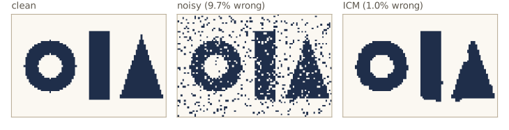
The energy falls with every sweep, and ICM stops after a few sweeps with roughly a tenth of the original error rate. The remaining errors are along boundaries, where a pixel’s neighbors really do disagree, and at the sharp corner of the triangle, which the smoothness prior dislikes.
With \(h = 0\) and four neighbors, ICM’s decisions depend only on the ratio \(\eta / \beta\). A pixel ends up opposite to its observation \(y_j\) exactly when \(y_j \sum_k x_k < -\eta / \beta\). For an interior pixel, \(y_j \sum_k x_k\) can only be \(-4\), \(-2\), \(0\), \(2\), or \(4\) (four neighbors, each agreeing or disagreeing with \(y_j\)), so only three regimes exist:
for eta_try in (0.5, 1.5, 2.5, 4.5):
    x_try = icm(y_obs, 0.0, 1.0, eta_try)
    print(f"eta/beta = {eta_try}: {np.mean(x_try != x_true):.2%} of pixels wrong")
eta/beta = 0.5: 1.00% of pixels wrong
eta/beta = 1.5: 1.00% of pixels wrong
eta/beta = 2.5: 4.11% of pixels wrong
eta/beta = 4.5: 9.70% of pixels wrong
For \(\eta/\beta < 2\) a pixel follows the majority when at least three neighbors disagree with it; for \(2 < \eta/\beta < 4\) only when all four do, which fixes isolated pixels but not pairs; and for \(\eta/\beta > 4\) the data always win and ICM returns the noisy image unchanged. Setting \(\beta = 0\) has the same effect: with no links between pixels, the most probable image is \(\mathbf{x} = \mathbf{y}\).
In practice. ICM is fast but greedy. The max-sum algorithm later in this module usually finds better optima, and for energies of exactly this form (binary variables with neighbor terms that reward agreement) there are graph-cut algorithms, based on minimum cuts in a flow network, that find the global minimum exactly. They were a standard tool in computer vision for this reason.
Relation to directed graphs
How do we turn a Bayesian network into a Markov random field? For a chain \(x_1 \to x_2 \to \dots \to x_N\) it is easy: drop the arrows, and put each conditional into the potential of the link it lives on,
\[\psi_{1,2}(x_1, x_2) = p(x_1)\, p(x_2 \mid x_1), \qquad \psi_{n-1,n}(x_{n-1}, x_n) = p(x_n \mid x_{n-1}) \quad (n \ge 3),\]with \(Z = 1\). In general, each CPT \(p(x_k \mid \mathrm{pa}_k)\) must fit inside one clique of the undirected graph, so the node and all its parents must be linked to each other. For a node with one parent, dropping the arrow suffices. For a node with several parents we must add links between every pair of its parents. This is called moralization (“marrying the parents”), and the result, after dropping all arrows, is the moral graph. Then initialize all clique potentials to 1 and multiply each CPT into some clique that contains its family; \(Z = 1\) automatically.
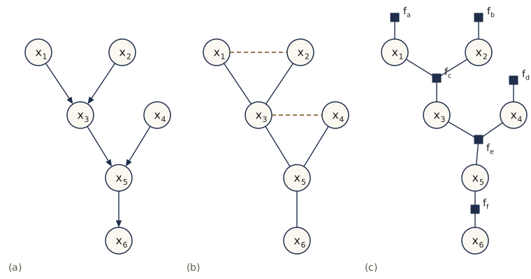
The undirected graph we used above is the moral graph of the polytree in panel (a). Let us moralize in code, turn random CPTs for the polytree into clique potentials, and confirm that the two representations define the same distribution. The variables have different numbers of states (two or three) so that any mix-up of axes would show.
poly_parents = {"x1": (), "x2": (), "x3": ("x1", "x2"), "x4": (), "x5": ("x3", "x4"), "x6": ("x5",)}
poly_states = {"x1": 2, "x2": 3, "x3": 2, "x4": 2, "x5": 3, "x6": 2}
poly_cpt = {v: rng.dirichlet(np.ones(poly_states[v]), size=tuple(poly_states[u] for u in pa))
            for v, pa in poly_parents.items()}
P_poly = joint_table(mrf_order, poly_parents, poly_cpt)

def moralize(parents):
    """Undirected moral graph: link each node to its parents, and marry every pair of parents."""
    edges = [(u, v) for v, pa in parents.items() for u in pa]
    edges += [(u, w) for pa in parents.values() for u, w in combinations(pa, 2)]
    adj = undirected(edges)
    for v in parents:
        adj.setdefault(v, set())
    return adj

moral = moralize(poly_parents)
print("moral graph equals our undirected example:", moral == adj_u)
cl = [tuple(C) for C in maximal_cliques(moral)]
pot = {C: np.ones([poly_states[v] for v in C]) for C in cl}
for v, pa in poly_parents.items():
    fam = set(pa) | {v}
    C = next(C for C in cl if fam <= set(C))          # a maximal clique holding the family
    sub = [C.index(u) for u in pa + (v,)]
    pot[C] = np.einsum(pot[C], list(range(len(C))), poly_cpt[v], sub, list(range(len(C))))
ops = []
for C, table in pot.items():
    ops += [table, [midx[v] for v in C]]
joint_from_potentials = np.einsum(*ops, list(range(6)))
print(f"Z = {joint_from_potentials.sum():.6f};  largest difference from the DAG's joint: "
      f"{np.abs(joint_from_potentials - P_poly).max():.1e}")
print("x1, x2 d-separated in the DAG:", d_separated(poly_parents, ["x1"], ["x2"], []),
      "  separated in the moral graph:", separated(moral, ["x1"], ["x2"], []))
moral graph equals our undirected example: True
Z = 1.000000;  largest difference from the DAG's joint: 1.4e-17
x1, x2 d-separated in the DAG: True   separated in the moral graph: False
The last line shows the cost of moralization. In the DAG, \(x_1\) and \(x_2\) are independent (they meet head-to-head at \(x_3\)); in the moral graph they are linked, so that independence can no longer be read off. Moralization adds the fewest links needed to hold every CPT, and so it keeps as many independences as possible, but it can lose some. (Linking every pair of nodes would also hold every CPT, but it would lose all of them.) Going the other way, from undirected to directed, is rarely done, because the potentials would have to be turned into normalized conditionals.
Which graphs can say what. Call a graph a D-map (dependency map) of a distribution if every independence the distribution has is shown by the graph, and an I-map (independence map) if every independence the graph shows holds in the distribution. A graph with no links is a trivial D-map of anything; a fully connected graph is a trivial I-map of anything. A graph that is both is a perfect map. Directed and undirected graphs capture different families of perfect maps, and some distributions have neither:
- The head-to-head graph \(a \to c \leftarrow b\) is a perfect map for a distribution with \(a \perp\!\!\!\perp b\) but \(a \not\perp\!\!\!\perp b \mid c\). No undirected graph on three nodes says “independent, but dependent given \(c\)”.
- The undirected four-cycle \(a - c - b - d - a\) says \(a \perp\!\!\!\perp b \mid \{c, d\}\) and \(c \perp\!\!\!\perp d \mid \{a, b\}\), and nothing else. No DAG on four nodes implies exactly these two statements.
Graphs mixing directed and undirected links, called chain graphs, cover both kinds, but even they do not give every distribution a perfect map.
Inference in graphical models
Inference means computing the distribution of some variables given observed values of others. The simplest case is Bayes’ theorem on two nodes. The graph \(x \to y\) says \(p(x, y) = p(x)\, p(y \mid x)\). If we observe \(y\), we compute \(p(y) = \sum_{x'} p(y \mid x')\, p(x')\) and then \(p(x \mid y) = p(y \mid x)\, p(x) / p(y)\). The joint is now written as \(p(y)\, p(x \mid y)\), which is the graph \(y \to x\): inference reversed the arrow. Everything below scales this up without ever building the joint table.
Inference on a chain
Take an undirected chain of \(N\) nodes, each with \(K\) states (a directed chain converts to it without adding links):
\[p(\mathbf{x}) = \frac{1}{Z}\, \psi_{1,2}(x_1, x_2)\, \psi_{2,3}(x_2, x_3) \cdots \psi_{N-1,N}(x_{N-1}, x_N).\]We want the marginal \(p(x_n)\) of a node in the middle. By definition it is a sum over all the other variables, \(K^{N-1}\) terms for each value of \(x_n\). The trick is to push each sum as far right as it will go. Only \(\psi_{1,2}\) involves \(x_1\), so sum over \(x_1\) first; the result is a function of \(x_2\), which together with \(\psi_{2,3}\) is all that involves \(x_2\); and so on from both ends:
\[p(x_n) = \frac{1}{Z} \underbrace{\Big[\sum_{x_{n-1}} \psi_{n-1,n}(x_{n-1}, x_n) \cdots \Big[\sum_{x_1} \psi_{1,2}(x_1, x_2)\Big] \cdots\Big]}_{\mu_\alpha(x_n)} \underbrace{\Big[\sum_{x_{n+1}} \psi_{n,n+1}(x_n, x_{n+1}) \cdots \Big[\sum_{x_N} \psi_{N-1,N}(x_{N-1}, x_N)\Big] \cdots\Big]}_{\mu_\beta(x_n)} .\]The only law used is distributivity, \(ab + ac = a(b + c)\): the right side does the same work with one fewer multiplication, and nested over the whole chain that saving becomes exponential.
The two brackets can be computed recursively, as messages passed along the chain. The forward message into \(x_n\) comes from the message into \(x_{n-1}\), and the backward message into \(x_n\) from the one into \(x_{n+1}\):
\[\mu_\alpha(x_n) = \sum_{x_{n-1}} \psi_{n-1,n}(x_{n-1}, x_n)\, \mu_\alpha(x_{n-1}), \qquad \mu_\beta(x_n) = \sum_{x_{n+1}} \psi_{n,n+1}(x_n, x_{n+1})\, \mu_\beta(x_{n+1}),\]starting from \(\mu_\alpha(x_1) = 1\) and \(\mu_\beta(x_N) = 1\). Each message is a vector of \(K\) numbers, and each step is a vector–matrix product costing \(O(K^2)\). Then
\[p(x_n) = \frac{1}{Z}\, \mu_\alpha(x_n)\, \mu_\beta(x_n), \qquad Z = \sum_{x_n} \mu_\alpha(x_n)\, \mu_\beta(x_n)\]for any \(n\). One forward pass and one backward pass, storing all messages, give every marginal at once for \(O(NK^2)\) work. Neighboring pairs come for free as well:
\[p(x_{n-1}, x_n) = \frac{1}{Z}\, \mu_\alpha(x_{n-1})\, \psi_{n-1,n}(x_{n-1}, x_n)\, \mu_\beta(x_n).\]Evidence. If \(x_m\) is observed to equal \(\hat{x}_m\), multiply the joint by an indicator \(I(x_m, \hat{x}_m)\), which is 1 at the observed value and 0 elsewhere. The sums over \(x_m\) then collapse to one term, and the same message passing gives \(p(x_n, \hat{x}_m)\), whose normalizer is the probability of the evidence. In code it is convenient to allow a vector of unary factors \(\phi_n(x_n)\) on each node, all ones by default and an indicator for an observed node.
def chain_messages(psi, phi=None):
    """Forward and backward messages on a chain. psi[n] is the K x K table of psi_{n,n+1}
    (0-based); phi is an optional (N, K) array of unary factors (e.g. evidence indicators)."""
    N, K = len(psi) + 1, psi[0].shape[0]
    phi = np.ones((N, K)) if phi is None else phi
    mu_a, mu_b = np.ones((N, K)), np.ones((N, K))
    for n in range(1, N):
        mu_a[n] = (mu_a[n - 1] * phi[n - 1]) @ psi[n - 1]     # sum over x_{n-1}
    for n in range(N - 2, -1, -1):
        mu_b[n] = psi[n] @ (phi[n + 1] * mu_b[n + 1])         # sum over x_{n+1}
    return mu_a, mu_b, phi

def chain_marginals(psi, phi=None):
    mu_a, mu_b, phi = chain_messages(psi, phi)
    unnorm = mu_a * phi * mu_b
    Z = unnorm[0].sum()
    pairs = [mu_a[n][:, None] * phi[n][:, None] * psi[n] * (phi[n + 1] * mu_b[n + 1])[None, :] / Z
             for n in range(len(psi))]
    return unnorm / Z, pairs, Z, unnorm.sum(axis=1)

def chain_joint(psi):
    """Brute force: the full K^N table of the unnormalized chain distribution."""
    N = len(psi) + 1
    ops = []
    for n, t in enumerate(psi):
        ops += [t, [n, n + 1]]
    return np.einsum(*ops, list(range(N)))

rng_chain = np.random.default_rng(80)
N, K = 8, 3
psi_c = [np.exp(rng_chain.normal(size=(K, K))) for _ in range(N - 1)]
marg_c, pairs_c, Z_c, Z_each = chain_marginals(psi_c)
J = chain_joint(psi_c)
brute = [J.sum(axis=tuple(m for m in range(N) if m != n)) / J.sum() for n in range(N)]
print(f"Z from messages {Z_c:.6f}, by brute force {J.sum():.6f};  Z at every node equal:",
      np.allclose(Z_each, Z_c))
err = max(np.abs(marg_c[n] - brute[n]).max() for n in range(N))
print(f"largest error over all {N} marginals: {err:.1e}")
p34 = J.sum(axis=tuple(m for m in range(N) if m not in (3, 4))) / J.sum()
print(f"largest error in p(x4, x5): {np.abs(pairs_c[3] - p34).max():.1e}")

phi_ev = np.ones((N, K))
phi_ev[5] = [0, 0, 1]                                   # observe x6 = 2 (0-based node 5)
marg_ev, _, Z_ev, _ = chain_marginals(psi_c, phi_ev)
J_ev = J[:, :, :, :, :, 2, :, :]
p_x2_ev = J_ev.sum(axis=(0, 2, 3, 4, 5, 6)) / J_ev.sum()
print("p(x2 | x6 = 2): messages", marg_ev[1], " brute force", p_x2_ev)
print(f"p(x6 = 2) = {Z_ev / Z_c:.4f}  (brute force {J_ev.sum() / J.sum():.4f})")
Z from messages 340625.506054, by brute force 340625.506054;  Z at every node equal: True
largest error over all 8 marginals: 6.7e-16
largest error in p(x4, x5): 1.1e-16
p(x2 | x6 = 2): messages [0.1122 0.2468 0.6411]  brute force [0.1122 0.2468 0.6411]
p(x6 = 2) = 0.7126  (brute force 0.7126)
Every marginal, the pairwise marginal, the conditional given evidence, and the probability of the evidence agree with brute force, and every node gives the same \(Z\). Now the cost. Brute force touches all \(K^N\) joint states; message passing performs about \(2(N-1)K^2\) multiply–adds.
print(f"{'N':>4s} {'K^N (brute force)':>22s} {'2(N-1)K^2 (messages)':>22s}")
for n_ in (8, 20, 50, 100):
    print(f"{n_:4d} {float(K)**n_:22.3g} {2 * (n_ - 1) * K**2:22d}")

psi_12 = [np.exp(rng_chain.normal(size=(K, K))) for _ in range(11)]    # N = 12
t0 = perf_counter()
m_brute = chain_joint(psi_12).sum(axis=tuple(range(1, 12)))           # p(x1) by brute force
t_b = perf_counter() - t0
t0 = perf_counter()
m_msg = chain_marginals(psi_12)[0]                                     # all twelve marginals
t_m = perf_counter() - t0
print(f"N = 12: brute force {t_b * 1e3:.1f} ms for one marginal, "
      f"messages {t_m * 1e3:.2f} ms for all twelve; "
      f"agree: {np.allclose(m_brute / m_brute.sum(), m_msg[0])}")
   N      K^N (brute force)   2(N-1)K^2 (messages)
   8               6.56e+03                    126
  20               3.49e+09                    342
  50               7.18e+23                    882
 100               5.15e+47                   1782
N = 12: brute force 13.4 ms for one marginal, messages 0.17 ms for all twelve; agree: True
Linear versus exponential. (The timings are from one run and your times will differ, but the ratio grows by a factor of about \(K\) with every node added.) At \(N = 20\) the brute-force table would already have billions of entries, while the messages need a few hundred operations.
Watch out. On long chains the raw messages overflow or underflow: each is a product of many potentials, so it grows or shrinks geometrically with \(n\). The standard fix is to normalize each message to sum to one as you go and keep the logarithms of the normalizers, whose sum is \(\ln Z\). The next cell shows the problem and the fix; the scaled forward–backward recursions of module 13 are the same idea.
def chain_log_Z(psi):
    """ln Z from forward messages that are rescaled to sum to one at every step."""
    m, log_Z = np.ones(psi[0].shape[0]), 0.0
    for t in psi:
        m = m @ t
        log_Z += np.log(m.sum())
        m = m / m.sum()
    return log_Z + np.log(m.sum())

print(f"N = 8:    ln Z scaled {chain_log_Z(psi_c):.6f}, unscaled {np.log(Z_c):.6f}")
psi_long = [np.exp(rng_chain.normal(size=(K, K))) for _ in range(4999)]
with np.errstate(over="ignore"):
    unscaled = np.log(chain_messages(psi_long)[0][-1].sum())
    print(f"N = 5000: ln Z scaled {chain_log_Z(psi_long):.2f}, unscaled {unscaled:.2f}")
N = 8:    ln Z scaled 12.738539, unscaled 12.738539
N = 5000: ln Z scaled 7513.61, unscaled inf
Trees and polytrees
The chain result generalizes to any graph without loops. An undirected graph is a tree if there is exactly one path between any two nodes. A directed graph is a directed tree if one node, the root, has no parents and every other node has exactly one; moralizing it adds no links, so it becomes an undirected tree. A directed graph in which some nodes have several parents but there is still only one path between any two nodes (ignoring directions) is a polytree, like panel (a) of the last figure. A polytree has several parentless nodes, and its moral graph has loops, as panel (b) shows. The sum-product algorithm handles all three kinds, and the cleanest way to state it uses a third kind of graph.
Factor graphs
Directed and undirected graphs both express a joint distribution as a product of factors, each over a subset of the variables:
\[p(\mathbf{x}) = \prod_s f_s(\mathbf{x}_s).\]For a directed graph the factors are the CPTs; for an undirected graph they are the clique potentials (with \(1/Z\) as a factor over no variables). A factor graph draws this product literally. It has a circle for each variable, a small square for each factor, and a link from each factor to every variable it depends on. Links only ever join a variable to a factor, so the graph is bipartite.
A factor graph is more specific than the graphs it comes from. Several factors on the same variables stay separate, and different factor graphs can describe the same directed or undirected graph. For example, a fully connected undirected graph on three variables could come from one factor \(f(x_1, x_2, x_3)\) or from three pairwise factors \(f_a(x_1, x_2) f_b(x_1, x_3) f_c(x_2, x_3)\); the undirected graph cannot tell these apart, the factor graph can.
To convert an undirected graph, make one factor per maximal clique. To convert a directed graph, make one factor per CPT, linked to the node and its parents. Panel (c) of the polytree figure does this. The moral graph had loops, but the factor graph is a tree: the loop \(x_1 - x_2 - x_3\) becomes a single factor \(f_c\) touching all three variables. In the same way, a local cycle in a directed graph, such as \(x_1 \to x_2\), \(x_1 \to x_3\), \(x_2 \to x_3\), disappears if we group its CPTs into one factor. A factor graph is a tree when it has no loops, which for a connected graph means it has exactly one fewer link than nodes.
poly_factors = {"fa": (("x1",), poly_cpt["x1"]), "fb": (("x2",), poly_cpt["x2"]),
                "fc": (("x1", "x2", "x3"), poly_cpt["x3"]), "fd": (("x4",), poly_cpt["x4"]),
                "fe": (("x3", "x4", "x5"), poly_cpt["x5"]), "ff": (("x5", "x6"), poly_cpt["x6"])}
n_nodes = len(poly_factors) + len(mrf_order)
n_links = sum(len(vs) for vs, _ in poly_factors.values())
print(f"{n_nodes} nodes, {n_links} links: a tree (it is connected, and links = nodes - 1)")
12 nodes, 11 links: a tree (it is connected, and links = nodes - 1)
The sum-product algorithm
Now the main algorithm. We assume the factor graph is a tree and the variables are discrete (for continuous variables, sums become integrals; module 13 does the linear-Gaussian case). The goal is every marginal \(p(x) = \sum_{\mathbf{x} \setminus x} p(\mathbf{x})\), where \(\mathbf{x} \setminus x\) means all variables except \(x\).
Messages into a variable. Pick a variable node \(x\). Because the graph is a tree, cutting the links at \(x\) splits the rest into separate subtrees, one through each neighboring factor \(f_s\), \(s \in \operatorname{ne}(x)\). Group the factors accordingly: let \(F_s(x, X_s)\) be the product of all factors in the subtree hanging off \(f_s\), where \(X_s\) are that subtree’s variables. Then \(p(\mathbf{x}) = \prod_{s \in \operatorname{ne}(x)} F_s(x, X_s)\), the sets \(X_s\) do not overlap, and each sum can be moved inside its own group:
\[p(x) = \prod_{s \in \operatorname{ne}(x)} \Big[\sum_{X_s} F_s(x, X_s)\Big] = \prod_{s \in \operatorname{ne}(x)} \mu_{f_s \to x}(x), \qquad \mu_{f_s \to x}(x) \equiv \sum_{X_s} F_s(x, X_s).\]The marginal is the product of the messages arriving from the neighboring factors, each a vector over the values of \(x\).
Messages from factors. Let the other variables of \(f_s\) be \(x_1, \dots, x_M\). The subtree behind \(f_s\) is the factor itself times one smaller subtree behind each \(x_m\), with product \(G_m(x_m, X_{sm})\):
\[F_s(x, X_s) = f_s(x, x_1, \dots, x_M)\, G_1(x_1, X_{s1}) \cdots G_M(x_M, X_{sM}).\]Summing, and again moving each sum inside its group,
\[\mu_{f_s \to x}(x) = \sum_{x_1} \cdots \sum_{x_M} f_s(x, x_1, \dots, x_M) \prod_{m \in \operatorname{ne}(f_s) \setminus x} \mu_{x_m \to f_s}(x_m), \qquad \mu_{x_m \to f_s}(x_m) \equiv \sum_{X_{sm}} G_m(x_m, X_{sm}).\]In words: multiply the factor by the messages coming in on all its other links, then sum out every variable except the one you are sending to.
Messages from variables. The subtree behind \(x_m\) consists of the subtrees behind each of its other factors \(f_l\), so \(G_m(x_m, X_{sm})\) is the product of the \(F_l(x_m, X_{ml})\) over \(l \in \operatorname{ne}(x_m) \setminus f_s\), and
\[\mu_{x_m \to f_s}(x_m) = \prod_{l \in \operatorname{ne}(x_m) \setminus f_s} \mu_{f_l \to x_m}(x_m).\]A variable just multiplies the messages from its other factors; one with only two neighbors passes messages through unchanged.
Leaves. The recursion ends at the leaves. A leaf variable sends \(\mu_{x \to f}(x) = 1\) (an empty product), and a leaf factor on a single variable sends \(\mu_{f \to x}(x) = f(x)\). Collecting the two rules in one place:
\[\mu_{f \to x}(x) = \sum_{\mathbf{x}_f \setminus x} f(\mathbf{x}_f) \prod_{m \in \operatorname{ne}(f) \setminus x} \mu_{x_m \to f}(x_m), \qquad \mu_{x \to f}(x) = \prod_{l \in \operatorname{ne}(x) \setminus f} \mu_{f_l \to x}(x).\]Result. On a tree-structured factor graph, the sum-product algorithm computes the two kinds of message above, starting from the leaves. Then \(p(x) \propto \prod_{s \in \operatorname{ne}(x)} \mu_{f_s \to x}(x)\) for every variable, and \(p(\mathbf{x}_s) \propto f_s(\mathbf{x}_s) \prod_{i \in \operatorname{ne}(f_s)} \mu_{x_i \to f_s}(x_i)\) for the variables of every factor.
Schedule. A node can send a message on a link as soon as it has heard from all its other links. Pick any node as the root. Messages flow inward from the leaves until the root has heard from every neighbor, and then outward again until every leaf has been reached. After that, a message has crossed every link once in each direction, every node has heard from all its neighbors, and every marginal is available. That is twice the number of links in messages, only twice the cost of one marginal. (The root is only a bookkeeping device; the messages do not depend on it.)
Normalization and evidence. If the factor graph came from a directed graph, \(Z = 1\) and the results are already normalized. If it came from an undirected graph, run the algorithm on the unnormalized product and normalize any one marginal at the end, a sum over one variable, to find \(Z\). Observed variables are handled as on the chain: multiply in indicator factors, and the normalizer becomes the probability of the evidence.
Our implementation lets each message request the messages it depends on, recursively, and caches every message the first time it is computed. On a tree the requests always bottom out at the leaves, and asking for every marginal ends up computing each of the \(2 \times\)(number of links) messages exactly once, in a valid order, without writing the schedule down. (On a graph with loops the recursion would never end; that is the subject of loopy belief propagation below.)
def factor_message(f_vars, table, x, incoming):
    """Message from a factor to its variable x: multiply the table by the incoming messages
    from the factor's other variables (broadcast along their axes), then sum those axes out."""
    prod = table
    for ax, v in enumerate(f_vars):
        if v != x:
            shape = [1] * len(f_vars)
            shape[ax] = -1
            prod = prod * incoming[v].reshape(shape)
    keep = f_vars.index(x)
    return prod.sum(axis=tuple(a for a in range(len(f_vars)) if a != keep))

def neighbors(factors):
    """variable -> list of the factors that mention it."""
    nb = {}
    for f, (vs, _) in factors.items():
        for v in vs:
            nb.setdefault(v, []).append(f)
    return nb

def sum_product(factors):
    """Marginals of every variable and every factor's variables on a tree-structured factor graph.
    factors: {name: (tuple of variable names, table with one axis per variable)}."""
    nb = neighbors(factors)
    size = {v: factors[fs[0]][1].shape[factors[fs[0]][0].index(v)] for v, fs in nb.items()}
    msg = {}                                        # msg[(sender, receiver)]

    def var_to_factor(x, f):
        if (x, f) not in msg:
            m = np.ones(size[x])                    # a leaf variable sends ones
            for g in nb[x]:
                if g != f:
                    m = m * factor_to_var(g, x)
            msg[(x, f)] = m
        return msg[(x, f)]

    def factor_to_var(f, x):
        if (f, x) not in msg:
            vs, table = factors[f]
            incoming = {v: var_to_factor(v, f) for v in vs if v != x}
            msg[(f, x)] = factor_message(vs, table, x, incoming)
        return msg[(f, x)]

    var_marg = {x: np.prod([factor_to_var(f, x) for f in nb[x]], axis=0) for x in nb}
    fac_marg = {}
    for f, (vs, table) in factors.items():
        prod = table
        for ax, v in enumerate(vs):
            shape = [1] * len(vs)
            shape[ax] = -1
            prod = prod * var_to_factor(v, f).reshape(shape)
        fac_marg[f] = prod
    Z = next(iter(var_marg.values())).sum()
    return ({x: m / Z for x, m in var_marg.items()}, {f: t / Z for f, t in fac_marg.items()},
            Z, len(msg))

def brute_joint(factors, order):
    idx = {v: i for i, v in enumerate(order)}
    ops = []
    for vs, table in factors.values():
        ops += [table, [idx[v] for v in vs]]
    return np.einsum(*ops, list(range(len(order))))
We run it on the factor graph of the polytree, compare every variable marginal and the three-variable marginal of factor \(f_e\) with brute force, and read off the pairwise marginal \(p(x_3, x_5)\) by summing \(x_4\) out of the factor marginal. Then we observe \(x_6 = 1\) by adding an indicator factor.
marg_sp, fmarg_sp, Z_sp, n_msgs = sum_product(poly_factors)
PJ = brute_joint(poly_factors, mrf_order)
print(f"messages computed: {n_msgs} (= 2 x {n_links} links);  Z = {Z_sp:.6f}")
err = max(np.abs(marg_sp[v] - marginal(PJ, mrf_order, [v])).max() for v in mrf_order)
print(f"largest error over all six variable marginals: {err:.1e}")
print(f"largest error in p(x3, x4, x5) from factor fe: "
      f"{np.abs(fmarg_sp['fe'] - marginal(PJ, mrf_order, ['x3', 'x4', 'x5'])).max():.1e}")
print("p(x3, x5) from the factor marginal:\n", fmarg_sp["fe"].sum(axis=1))

obs_factors = dict(poly_factors, obs=(("x6",), np.array([0.0, 1.0])))    # indicator for x6 = 1
marg_obs, _, Z_obs, _ = sum_product(obs_factors)
PJ6 = PJ[..., 1] / PJ[..., 1].sum()                   # brute force: p(x1..x5 | x6 = 1)
err = max(np.abs(marg_obs[v] - marginal(PJ6, mrf_order[:5], [v])).max() for v in mrf_order[:5])
print(f"with x6 = 1 observed: largest error {err:.1e};  p(x6 = 1) = {Z_obs:.4f} "
      f"(brute force {PJ[..., 1].sum():.4f})")
print("p(x2) before and after observing x6 = 1:", marg_sp["x2"], marg_obs["x2"])
messages computed: 22 (= 2 x 11 links);  Z = 1.000000
largest error over all six variable marginals: 3.3e-16
largest error in p(x3, x4, x5) from factor fe: 2.8e-17
p(x3, x5) from the factor marginal:
 [[0.0487 0.0284 0.1633]
 [0.3256 0.1836 0.2505]]
with x6 = 1 observed: largest error 1.1e-16;  p(x6 = 1) = 0.2252 (brute force 0.2252)
p(x2) before and after observing x6 = 1: [0.0295 0.4556 0.5149] [0.0295 0.4495 0.521 ]
All marginals match brute force to round-off, with exactly 22 messages for 11 links. With the factor graph from a directed model, \(Z = 1\); with the evidence factor added, the normalizer is the probability of the evidence. The last line shows evidence traveling up the tree. The path from \(x_2\) to \(x_6\) in the DAG is \(x_2 \to x_3 \to x_5 \to x_6\), head-to-tail at both \(x_3\) and \(x_5\), and neither is observed, so the path is open and observing \(x_6\) changes our beliefs about \(x_2\). The same observation also couples \(x_2\) and \(x_4\), which are independent a priori: their only path meets head-to-head at \(x_5\), and \(x_6\) is a descendant of \(x_5\).
Belief propagation, the message-passing algorithm for directed trees and polytrees that predates factor graphs, is a special case of sum-product. Likewise, running sum-product on the chain’s factor graph (one factor per link) reproduces the \(\mu_\alpha\) and \(\mu_\beta\) recursions exactly (exercise 7).
The max-sum algorithm
Marginals answer “how likely is each value of each variable”. A different question is “which joint configuration is most likely”:
\[\mathbf{x}^{\max} = \arg\max_{\mathbf{x}} p(\mathbf{x}), \qquad p(\mathbf{x}^{\max}) = \max_{\mathbf{x}} p(\mathbf{x}).\]It is tempting to take each variable’s most probable value from its marginal, but that answers a different question and can give a poor joint configuration:
p_xy = np.array([[0.35, 0.05],      # rows x = 0, 1; columns y = 0, 1
                 [0.30, 0.30]])
x_hat, y_hat = p_xy.sum(1).argmax(), p_xy.sum(0).argmax()
i, j = np.unravel_index(p_xy.argmax(), p_xy.shape)
print(f"marginals p(x) = {p_xy.sum(1)}, p(y) = {p_xy.sum(0)}")
print(f"most probable value of each marginal: (x, y) = ({x_hat}, {y_hat}), "
      f"joint probability {p_xy[x_hat, y_hat]:.2f}")
print(f"most probable joint configuration:    (x, y) = ({i}, {j}), "
      f"joint probability {p_xy[i, j]:.2f}")
marginals p(x) = [0.4 0.6], p(y) = [0.65 0.35]
most probable value of each marginal: (x, y) = (1, 0), joint probability 0.30
most probable joint configuration:    (x, y) = (0, 0), joint probability 0.35
For the joint maximum we reuse the sum-product derivation with sums replaced by maxima. It works because the max also distributes over products of nonnegative numbers, \(\max(ab, ac) = a \max(b, c)\) for \(a \ge 0\). On the chain,
\[\max_{\mathbf{x}} p(\mathbf{x}) = \frac{1}{Z} \max_{x_N} \Big[\max_{x_{N-1}} \psi_{N-1,N}(x_{N-1}, x_N) \cdots \Big[\max_{x_1} \psi_{1,2}(x_1, x_2)\Big] \cdots \Big].\]Products of many probabilities underflow, so we work with logarithms. The log is increasing, so \(\ln \max_{\mathbf{x}} p(\mathbf{x}) = \max_{\mathbf{x}} \ln p(\mathbf{x})\), and the distributive law becomes \(\max(a + b, a + c) = a + \max(b, c)\). Replacing sums by maxima and products by sums of logs in the sum-product messages gives the max-sum algorithm:
\[\mu_{f \to x}(x) = \max_{\mathbf{x}_f \setminus x} \Big[\ln f(\mathbf{x}_f) + \sum_{m \in \operatorname{ne}(f) \setminus x} \mu_{x_m \to f}(x_m)\Big], \qquad \mu_{x \to f}(x) = \sum_{l \in \operatorname{ne}(x) \setminus f} \mu_{f_l \to x}(x),\]with leaf messages \(\mu_{x \to f}(x) = 0\) and \(\mu_{f \to x}(x) = \ln f(x)\). After passing messages from the leaves to a root variable \(x\), the maximum of \(\sum_{s \in \operatorname{ne}(x)} \mu_{f_s \to x}(x)\) over \(x\) is \(\max_{\mathbf{x}} \ln p(\mathbf{x})\) (plus \(\ln Z\) for an undirected model), and the maximizing value of the root is the argmax.
Back-tracking. For the other variables we should not send messages back out and take each node’s argmax separately: if several joint configurations tie for the maximum, the per-node choices can come from different ones and together not be a maximizer. Instead, during the inward pass each factor records which values of its other variables achieved the maximum. On the chain with root \(x_N\), the message into \(x_n\) and its record are
\[\omega(x_n) = \max_{x_{n-1}} \big[\ln \psi_{n-1,n}(x_{n-1}, x_n) + \omega(x_{n-1})\big], \qquad \phi(x_n) = \arg\max_{x_{n-1}} \big[\ln \psi_{n-1,n}(x_{n-1}, x_n) + \omega(x_{n-1})\big],\]with \(\omega(x_1) = 0\). Once \(x_N^{\max} = \arg\max \omega(x_N)\) is known, follow the records backward: \(x_{n-1}^{\max} = \phi(x_n^{\max})\). This is back-tracking, and it always returns one consistent maximizing configuration. On a hidden Markov model it is the Viterbi algorithm of module 13; it is also exactly dynamic programming.
def max_sum_chain(log_psi):
    """Most probable configuration of a chain, and the max of sum_n ln psi_n, by max-sum."""
    omega, phi = np.zeros(log_psi[0].shape[0]), []
    for lp in log_psi:
        s = omega[:, None] + lp                 # s[x_{n-1}, x_n]
        phi.append(s.argmax(axis=0))            # best predecessor for each value of x_n
        omega = s.max(axis=0)
    x = [int(omega.argmax())]
    for ph in reversed(phi):                    # back-tracking
        x.append(int(ph[x[-1]]))
    return x[::-1], omega.max()

x_ms, best = max_sum_chain([np.log(t) for t in psi_c])
x_bf = np.unravel_index(J.argmax(), J.shape)
print("max-sum:    ", x_ms, f"  ln p = {best - np.log(Z_c):.4f}")
print("brute force:", [int(v) for v in x_bf], f"  ln p = {np.log(J.max() / Z_c):.4f}")
print("each marginal's most probable value:", [int(m.argmax()) for m in marg_c])

agree = 0
for _ in range(200):
    ps = [np.exp(rng_chain.normal(size=(3, 3))) for _ in range(6)]
    xm, _ = max_sum_chain([np.log(t) for t in ps])
    Jr = chain_joint(ps)
    agree += tuple(xm) == tuple(int(v) for v in np.unravel_index(Jr.argmax(), Jr.shape))
print(f"random chains with N = 7, K = 3: max-sum found the brute-force argmax in {agree} of 200")
max-sum:     [1, 2, 2, 1, 1, 2, 1, 1]   ln p = -3.2071
brute force: [1, 2, 2, 1, 1, 2, 1, 1]   ln p = -3.2071
each marginal's most probable value: [1, 2, 2, 1, 1, 2, 2, 1]
random chains with N = 7, K = 3: max-sum found the brute-force argmax in 200 of 200
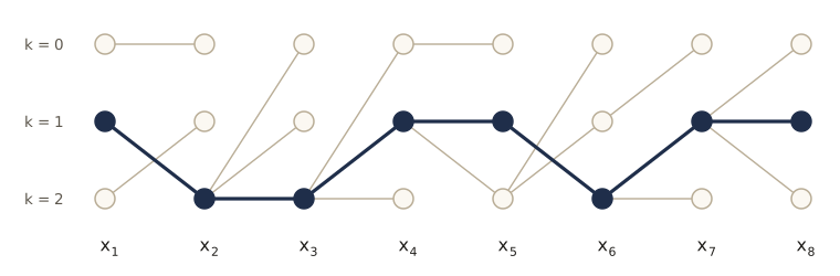
Max-sum agrees with brute force on every chain. Notice also that the most probable values of the individual marginals differ from the most probable configuration at \(x_7\). The figure draws the records \(\phi\) as a trellis, a diagram whose nodes are the individual states of the variables (so it is not itself a graphical model). Every state in a column has exactly one line back, so back-tracking from any final state traces a unique path.
On a general tree the procedure is the same: each factor-to-variable message records the maximizing values of the factor’s other variables, and back-tracking from the root assigns them consistently. Evidence is again handled by clamping observed variables.
Max-sum and ICM both look for a high-probability configuration, but differently. ICM passes a single value between neighbors and settles for a local optimum. Max-sum passes a whole vector of \(K\) values per message and is exact on any tree. On a longer chain, where we can no longer check by brute force but max-sum is still exact, ICM from random starts tends to stall:
def icm_chain(log_psi, x, max_sweeps=100):
    """ICM on a chain: set each x_n to its best value given its two neighbors, until stable."""
    x, N = list(x), len(log_psi) + 1
    for _ in range(max_sweeps):
        changed = False
        for n in range(N):
            score = np.zeros(log_psi[0].shape[0])
            if n > 0:
                score += log_psi[n - 1][x[n - 1], :]
            if n < N - 1:
                score += log_psi[n][:, x[n + 1]]
            new = int(score.argmax())
            changed |= new != x[n]
            x[n] = new
        if not changed:
            break
    return x

def chain_log_score(log_psi, x):
    return sum(lp[x[n], x[n + 1]] for n, lp in enumerate(log_psi))

lp30 = [rng_chain.normal(size=(4, 4)) for _ in range(29)]              # N = 30, K = 4
_, best30 = max_sum_chain(lp30)
scores = np.array([chain_log_score(lp30, icm_chain(lp30, rng_chain.integers(0, 4, size=30)))
                   for _ in range(50)])
print(f"max-sum log score {best30:.3f};  ICM from 50 random starts: best {scores.max():.3f}, "
      f"median {np.median(scores):.3f}, "
      f"reached the maximum {np.isclose(scores, best30).sum()} times")
max-sum log score 43.923; ICM from 50 random starts: best 42.000, median 37.386, reached the maximum 0 times
ICM never reached the maximum in 50 starts, and its median run falls well short: each run stopped at a configuration that no single-variable change could improve, even though changing several variables at once would.
Exact inference in general graphs
Sum-product and max-sum are exact on trees. Many useful graphs have loops, such as the pixel grid of the de-noising model. The junction tree algorithm extends exact message passing to any graph by grouping variables until the graph becomes a tree. In outline:
- If the graph is directed, moralize it.
- Triangulate: add links until every cycle of four or more nodes has a chord (a link between two nodes of the cycle that are not neighbors on it). For the four-cycle \(a - c - b - d - a\), add the link \(a - b\) or \(c - d\).
- Build a tree whose nodes are the maximal cliques of the triangulated graph. Among all trees that connect the cliques, choose one that maximizes the total weight, where a link’s weight is the number of variables the two cliques share. After absorbing any clique contained in another, this is the junction tree.
- Run a two-pass message-passing algorithm, essentially sum-product, on the junction tree.
The triangulation guarantees the running intersection property: a variable that appears in two cliques appears in every clique on the path between them, which keeps the messages consistent. The algorithm is exact for any graph, but each message is a table over a whole clique, so the cost grows exponentially with the size of the largest clique. The treewidth of a graph is the size of the largest clique, minus one, in the best junction tree we could build for it (the minus one makes a tree’s treewidth equal to 1). For graphs with large treewidth, such as a large grid, exact inference is out of reach, and we need approximations.
Loopy belief propagation
The simplest approximation is to run sum-product anyway on a graph with loops. The message rules are local, so nothing stops us; the question is only what the result means. This is loopy belief propagation.
On a graph with loops no node ever hears from all its other links first, so we initialize every message to the all-ones vector and then update repeatedly according to a schedule. The flooding schedule updates every message in both directions at each step from the previous step’s messages; serial schedules send one message at a time. A message is pending on a link if the sender has received something new on its other links since it last sent on that one. On a tree, the pending messages run out after a finite number of steps, and the result is exact. On a graph with loops information keeps circulating, and the messages may or may not settle down. When they do, the beliefs (products of incoming messages, normalized) are often good approximations to the marginals, but they are not exact.
Our flooding implementation reuses factor_message and normalizes every message to sum to one (only their direction matters). We first run it on the polytree’s factor graph, where it must reproduce the exact marginals, and then on a \(3 \times 3\) grid of binary spins \(s_i \in \{-1, +1\}\) with random fields \(h_i\) and a common coupling \(J\): \(p(\mathbf{s}) \propto \exp\big(\sum_i h_i s_i + J \sum_{\{i,j\}} s_i s_j\big)\), a small cousin of the de-noising model.
def loopy_bp(factors, max_iters=500, tol=1e-10):
    """Sum-product with the flooding schedule; exact on trees, approximate with loops."""
    nb = neighbors(factors)
    size = {v: factors[fs[0]][1].shape[factors[fs[0]][0].index(v)] for v, fs in nb.items()}
    m_vf = {(x, f): np.ones(size[x]) / size[x] for x in nb for f in nb[x]}
    m_fv = {(f, x): np.ones(size[x]) / size[x] for x in nb for f in nb[x]}
    for it in range(1, max_iters + 1):
        new_vf = {}
        for x, f in m_vf:
            m = np.prod([m_fv[(g, x)] for g in nb[x] if g != f] or [np.ones(size[x])], axis=0)
            new_vf[(x, f)] = m / m.sum()
        new_fv = {}
        for f, x in m_fv:
            vs, table = factors[f]
            m = factor_message(vs, table, x, {v: m_vf[(v, f)] for v in vs if v != x})
            new_fv[(f, x)] = m / m.sum()
        change = max(max(np.abs(new_vf[k] - m_vf[k]).max() for k in m_vf),
                     max(np.abs(new_fv[k] - m_fv[k]).max() for k in m_fv))
        m_vf, m_fv = new_vf, new_fv
        if change < tol:
            break
    beliefs = {x: np.prod([m_fv[(f, x)] for f in nb[x]], axis=0) for x in nb}
    return {x: b / b.sum() for x, b in beliefs.items()}, it, change < tol

bel, iters, ok = loopy_bp(poly_factors)
err = max(np.abs(bel[v] - marg_sp[v]).max() for v in mrf_order)
print(f"polytree (a tree): converged {ok} after {iters} rounds, largest error {err:.1e}")

rng_grid = np.random.default_rng(88)
cells = [(i, j) for i in range(3) for j in range(3)]
names = {c: f"s{c[0]}{c[1]}" for c in cells}
h_grid = rng_grid.normal(0, 0.5, size=9)
spin = np.array([-1.0, 1.0])
for J_c in (0.2, 0.5, 1.0):
    grid = {f"h{names[c]}": ((names[c],), np.exp(h_grid[k] * spin)) for k, c in enumerate(cells)}
    for (i, j) in cells:
        for (di, dj) in ((0, 1), (1, 0)):
            if i + di < 3 and j + dj < 3:
                a, b = names[(i, j)], names[(i + di, j + dj)]
                grid[f"J{a}{b}"] = ((a, b), np.exp(J_c * np.outer(spin, spin)))
    order_g = [names[c] for c in cells]
    PG = brute_joint(grid, order_g)
    PG = PG / PG.sum()
    bel, iters, ok = loopy_bp(grid)
    err = max(np.abs(bel[v] - marginal(PG, order_g, [v])).max() for v in order_g)
    print(f"3 x 3 grid, J = {J_c}: converged {ok} after {iters:3d} rounds, "
          f"largest error in a marginal {err:.4f}")
polytree (a tree): converged True after 8 rounds, largest error 1.1e-16
3 x 3 grid, J = 0.2: converged True after  33 rounds, largest error in a marginal 0.0008
3 x 3 grid, J = 0.5: converged True after 113 rounds, largest error in a marginal 0.0270
3 x 3 grid, J = 1.0: converged True after  88 rounds, largest error in a marginal 0.3698
On the tree, flooding converges after a few rounds (about the diameter of the graph) to the exact marginals. On the grid it converges too, with errors that grow with the coupling: weak couplings let little information go around the loops, strong ones let the same evidence be counted repeatedly. Loopy belief propagation can fail badly on some models and is remarkably good on others; the best-known success is the decoding of modern error-correcting codes, such as turbo codes and low-density parity-check codes, which is equivalent to loopy belief propagation on the code’s factor graph. Module 10 develops approximate inference more systematically.
Learning the graph structure
So far the graph was given. We can also try to learn it from data. That needs a space of candidate structures and a score for each. The Bayesian answer is a posterior over graphs \(m\),
\[p(m \mid \mathcal{D}) \propto p(m)\, p(\mathcal{D} \mid m),\]where the model evidence \(p(\mathcal{D} \mid m)\) (module 03) scores each structure and automatically penalizes needless complexity. Two things make this hard. Computing the evidence requires integrating over the parameters and summing over any latent variables. And the number of structures explodes. The number of undirected graphs on \(M\) labeled nodes is \(2^{M(M-1)/2}\), one choice per pair. DAGs are counted by a recursion due to Robinson that adds the parentless nodes one layer at a time:
\[a(M) = \sum_{k=1}^{M} (-1)^{k+1} \binom{M}{k}\, 2^{k(M-k)}\, a(M-k), \qquad a(0) = 1.\]def n_dags(M, memo={0: 1}):
"""Number of DAGs on M labeled nodes (Robinson's recursion)."""
if M not in memo:
memo[M] = sum((-1) ** (k + 1) * comb(M, k) * 2 ** (k * (M - k)) * n_dags(M - k)
for k in range(1, M + 1))
return memo[M]
for M in range(1, 9):
print(f"M = {M}: {2 ** (M * (M - 1) // 2):>12,d} undirected graphs {n_dags(M):>16,d} DAGs")
M = 1:            1 undirected graphs                 1 DAGs
M = 2:            2 undirected graphs                 3 DAGs
M = 3:            8 undirected graphs                25 DAGs
M = 4:           64 undirected graphs               543 DAGs
M = 5:        1,024 undirected graphs            29,281 DAGs
M = 6:       32,768 undirected graphs         3,781,503 DAGs
M = 7:    2,097,152 undirected graphs     1,138,779,265 DAGs
M = 8:  268,435,456 undirected graphs   783,702,329,343 DAGs
Even with eight variables there are hundreds of billions of DAGs, so structure learning relies on heuristic search, such as adding, deleting, or reversing one arrow at a time while the score improves.
Summary
| Idea | What it is | Key rule | Cost or guarantee |
|---|---|---|---|
| Bayesian network | DAG with one conditional per node | \(p(\mathbf{x}) = \prod_k p(x_k \mid \mathrm{pa}_k)\), normalized automatically | CPT size exponential in the number of parents |
| Linear-Gaussian network | each node Gaussian, mean linear in its parents | joint is Gaussian; mean and covariance by recursion | parameters between \(2D\) and \(D(D+3)/2\) |
| D-separation | reading independences off a DAG | tail-to-tail and head-to-tail nodes block when observed; head-to-head nodes block unless they or a descendant are observed | linear-time reachability search |
| Markov random field | undirected graph with clique potentials | \(p(\mathbf{x}) = \frac{1}{Z} \prod_C \psi_C(\mathbf{x}_C)\); independence by separation | \(Z\) sums over all \(K^M\) states |
| ICM | coordinate-wise maximization | set each variable to its best value given its neighbors | fast; local optimum only |
| Factor graph | bipartite graph of variables and factors | \(p(\mathbf{x}) = \prod_s f_s(\mathbf{x}_s)\) | a polytree becomes a tree |
| Sum-product | messages that sum out variables | factor: multiply and sum; variable: multiply | exact marginals on trees; \(O(NK^2)\) on a chain |
| Max-sum | messages that maximize, in log space | as sum-product with max and sums of logs, plus back-tracking | exact MAP configuration on trees |
| Junction tree | sum-product on a tree of cliques | moralize, triangulate, connect cliques | exact; exponential in the treewidth |
| Loopy belief propagation | sum-product on a graph with loops | iterate messages under a schedule | approximate; may not converge |
Ideas to carry forward:
- A graph is a statement about how a joint distribution factorizes, and equivalently about which conditional independences hold. The missing links carry the information.
- Observing a common cause or an intermediate variable blocks a path; observing a common effect opens one. The Markov blanket collects exactly what a node’s conditional depends on.
- Inference is sums of products, and on a tree the distributive law turns the exponential sum into local messages. Replacing the sum by a max gives the most probable configuration.
- These pieces reappear as the E step of EM (module 09), as the forward–backward and Viterbi algorithms (module 13), and as the starting point for approximate inference (modules 10 and 11).
Exercises
- For the chain \(x_1 \to x_2 \to x_3\) with linear-Gaussian conditionals, use the two recursions to derive \(\boldsymbol{\mu}\) and \(\boldsymbol{\Sigma}\) by hand in terms of \(b_i\), \(v_i\), \(w_{21}\), \(w_{32}\). Check your formulas with
lg_momentsfor numbers of your choice, and show that the \((1, 3)\) entry of the precision matrix is zero. Which independence statement does that zero express? - A noisy-OR conditional for a binary child with binary parents sets \(p(y = 0 \mid \mathbf{x})\) equal to \((1 - \lambda_0) \prod_{i} (1 - \lambda_i)^{x_i}\). Explain each parameter as the probability that one cause, acting alone, fails to trigger \(y\), and interpret \(\lambda_0\). How many parameters does it use compared with a full table? Write a function that builds the full CPT from \(\lambda_0, \dots, \lambda_M\), use it for \(L\) in the commute network, and recompute \(p(R = 1 \mid M = 1)\).
- Extend the autograder example with a node \(E\), an email from the course staff, where \(p(E = 1 \mid F = 1) = 0.9\) and \(p(E = 1 \mid F = 0) = 0.05\). Compute \(p(B = 1 \mid E = 1)\) and \(p(B = 1 \mid E = 1, S = 1)\). Explain with d-separation why observing \(E\) instead of \(F\) still produces explaining away, and why the effect is weaker.
- Prove with d-separation that a node is independent of all other nodes given its Markov blanket: consider every path leaving the node through a parent, through a child to a co-parent, and through a child to a grandchild. Then check it numerically: for 20 networks from
random_network, verify withd_separatedthat every node is d-separated from all non-blanket nodes by its blanket. - For the de-noising energy, prove that each ICM update never increases \(E\) and that ICM stops after finitely many sweeps. Then modify
icmto visit the pixels in a random order each sweep and to use the eight surrounding pixels as neighbors. How do the error rate and the \(\eta/\beta\) regimes change? - Suppose only the last node of a chain, \(x_N\), is observed. Show that the forward messages are unchanged and describe how the backward messages change. Use
chain_marginalsto compute \(p(x_n \mid x_N)\) for all \(n\) and check against brute force. - Build the factor graph of the eight-node chain (
psi_c), with one factor per link, and runsum_producton it. Show that its messages \(\mu_{f_{n-1,n} \to x_n}\) equal the forward messages fromchain_messages, and identify which messages equal the backward ones. - Two variables that do not share a factor, such as \(x_1\) and \(x_6\) in the polytree, have a joint marginal that sum-product does not give directly. Compute \(p(x_1, x_6)\) by clamping \(x_1\) to each of its values in turn, running
sum_productwith the indicator factor, and multiplying by the probability of the evidence. Check against brute force and count the messages used. - Construct a chain with \(N = 4\) and \(K = 2\) that has two different maximizing configurations. Compute “max-marginals” by running max-sum messages both forward and backward and taking each node’s argmax separately, and show that the result can be a configuration that is not a maximizer. Why does back-tracking avoid this?
- Run
loopy_bpon the \(3 \times 3\) grid with couplings of random sign (some \(J\) positive, some negative) and growing magnitude. Does it still converge? Try damping: replace each new message by a weighted average of the new and the old one. Report the largest error in the marginals as a function of the coupling strength. - Show that a distribution given by a directed tree can be written over the corresponding undirected tree with \(Z = 1\), and conversely that an undirected tree’s potentials can be renormalized into the CPTs of a directed tree. For an undirected tree with \(M\) nodes, how many different directed trees give the same undirected tree?
- In your own words: explain to a classmate why observing a common cause makes its effects independent, while observing a common effect makes its causes dependent, and how these two facts become the rules of d-separation.
Going further
- C. M. Bishop, Pattern Recognition and Machine Learning, chapter 8 — the source for this module. Exercises 8.3–8.4 check independences on a table, 8.10–8.11 add a descendant to a head-to-head node, 8.13–8.14 analyze ICM, 8.15–8.17 cover chains, 8.20–8.26 develop the sum-product algorithm, 8.27 shows that the most probable values of the marginals can have joint probability zero, and 8.28–8.29 are about pending messages.
- D. Koller and N. Friedman, Probabilistic Graphical Models: Principles and Techniques (MIT Press, 2009) — the comprehensive text, with full proofs of the d-separation and Hammersley–Clifford theorems, the reachability algorithm for d-separation, and the junction tree algorithm in detail.
- F. R. Kschischang, B. J. Frey, and H.-A. Loeliger, “Factor graphs and the sum-product algorithm”, IEEE Transactions on Information Theory, 2001 — the paper that made factor graphs standard, with many algorithms shown to be special cases of sum-product.
- M. J. Wainwright and M. I. Jordan, “Graphical models, exponential families, and variational inference”, Foundations and Trends in Machine Learning, 2008 — a long survey explaining loopy belief propagation and its relatives as variational methods; a good bridge to module 10.
- D. J. C. MacKay, Information Theory, Inference, and Learning Algorithms (Cambridge University Press, 2003; free to read on the author’s website) — its chapters on message passing and exact marginalization in graphs, and on error-correcting codes decoded by loopy belief propagation.
- J. Pearl, Probabilistic Reasoning in Intelligent Systems (Morgan Kaufmann, 1988) — the classic book on Bayesian networks, belief propagation, and d-separation.
These notes follow the chapters of C. M. Bishop, Pattern Recognition and Machine Learning (Springer, 2006), the course text, which Microsoft Research makes freely available as a PDF. The explanations, code, figures, and exercises here are written for this course; the book remains the reference, with the full derivations and many more exercises.