CSE 474/574 · Module 04 · Week 4
Linear Models for Classification
Discriminant functions, Fisher's discriminant, the perceptron, generative classifiers, logistic regression with IRLS, and the Laplace approximation.
Companion reading: Bishop, Pattern Recognition and Machine Learning, chapter 4, “Linear Models for Classification”
By the end of this module you can
- Explain the geometry of a linear discriminant — why \(\mathbf{w}\) is normal to the decision boundary and why \(y(\mathbf{x})/\lVert \mathbf{w} \rVert\) is a signed distance — and why a single \(K\)-class discriminant avoids the ambiguities of one-versus-the-rest and one-versus-one schemes.
- Fit a least-squares classifier in closed form and show, with an experiment, how outliers and a third class break it.
- Derive Fisher’s linear discriminant and its connection to least squares, and implement the perceptron and its convergence bound.
- Show that Gaussian class-conditional densities with a shared covariance give a posterior that is a logistic sigmoid (or softmax) of a linear function, fit such a model by maximum likelihood, and build a naive Bayes classifier for binary features.
- Derive the gradient and Hessian of the cross-entropy error for logistic and softmax regression, check them by finite differences, and fit both models with Newton’s method (IRLS).
- Explain why maximum likelihood fails on linearly separable data, what probit regression and canonical link functions are, and why the error-times-feature form of the gradient keeps reappearing.
- Build a Laplace approximation to a density and to a model’s evidence, and relate the evidence to the Bayesian information criterion.
- Compute the approximate predictive distribution of Bayesian logistic regression with the probit approximation, check it by Monte Carlo, and explain why its probabilities move toward one half away from the data.
Contents
- Classification with linear models
- Discriminant functions
- Probabilistic generative models
- Probabilistic discriminative models
- The Laplace approximation
- Bayesian logistic regression
- Summary
- Exercises
- Going further
In module 03 the target was a real number, and a model that is linear in its parameters gave us closed-form least-squares solutions, a clean Bayesian treatment, and the evidence for choosing between models. This module keeps the same building blocks — a linear function \(\mathbf{w}^{\mathrm{T}}\boldsymbol{\phi}(\mathbf{x})\) of fixed features — and asks them to predict a class label instead.
The change of target changes a surprising amount. A class label is not a noisy real number, so squared error turns out to be the wrong loss; probabilities must stay between 0 and 1, so the linear function has to pass through a squashing nonlinearity; and once that nonlinearity is there, the posterior over weights is no longer Gaussian and the tidy Bayesian results of module 03 need an approximation. We meet the three approaches to classification from the decision theory of module 01 one after another: discriminant functions that output a class directly, generative models that fit class-conditional densities with the Gaussians of module 02, and discriminative models, above all logistic regression, that fit the posterior class probabilities directly.
Along the way we build tools that the rest of the course leans on: Newton’s method for fitting (here called IRLS), the softmax function, and the Laplace approximation, which turns an awkward posterior into a Gaussian. Neural networks in module 05 are, at their output layer, exactly the models of this module with learned features.
Classification with linear models
We have an input vector \(\mathbf{x}\) with \(D\) components and \(K\) classes \(\mathcal{C}_1, \dots, \mathcal{C}_K\). A classifier divides input space into decision regions, one per class; the surfaces between regions are decision boundaries. A linear classifier is one whose decision boundaries are hyperplanes — flat surfaces of dimension \(D - 1\). When a data set can be classified without error by such hyperplanes, it is linearly separable.
How should we encode the class of a training point? For two classes we use a single binary target \(t \in \{0, 1\}\), with \(t = 1\) meaning \(\mathcal{C}_1\); it can be read as the probability that the class is \(\mathcal{C}_1\), which happens to be exactly 0 or 1 for a labeled point. For \(K > 2\) classes we use a 1-of-\(K\) coding: \(\mathbf{t}\) is a vector of length \(K\) with a single 1 in position \(k\) for class \(\mathcal{C}_k\) and zeros elsewhere. (The perceptron will use \(t \in \{-1, +1\}\) instead, which suits it better.)
Regression predicted \(y(\mathbf{x}) = \mathbf{w}^{\mathrm{T}}\mathbf{x} + w_0\), a number on the whole real line. For classification we want either a class label or a probability in \((0, 1)\), so we pass the linear function through a fixed nonlinearity \(f\):
\[y(\mathbf{x}) = f\left(\mathbf{w}^{\mathrm{T}}\mathbf{x} + w_0\right).\]In machine learning \(f\) is called the activation function; statisticians call its inverse \(f^{-1}\) the link function. Because \(f\) is monotonic, a surface of constant \(y\) is a surface of constant \(\mathbf{w}^{\mathrm{T}}\mathbf{x} + w_0\), which is a hyperplane: the decision boundaries stay linear in \(\mathbf{x}\) even though \(y\) is a nonlinear function. Models of this form are called generalized linear models. Note what we lose: \(y\) is no longer linear in \(\mathbf{w}\), so the closed-form solutions of module 03 are gone, except in the least-squares method we try first.
Everything in this module works the same way if \(\mathbf{x}\) is first replaced by a fixed feature vector \(\boldsymbol{\phi}(\mathbf{x})\), as in module 03. We start with raw inputs, where pictures are easier, and switch to \(\boldsymbol{\phi}\) for the probabilistic discriminative models.
The first code cell sets up NumPy and two small helpers used throughout: one prepends the constant input 1, one builds 1-of-\(K\) target vectors.
import numpy as np
from scipy.special import expit, logsumexp, log_ndtr, ndtr, erf
from scipy import stats

np.set_printoptions(precision=4, suppress=True)
rng = np.random.default_rng(474)

def add_bias(X):
    """Rows (1, x^T): the augmented inputs, so a bias is just one more weight."""
    return np.column_stack([np.ones(len(X)), X])

def one_hot(labels, K):
    """1-of-K target matrix T of shape (N, K) from integer labels 0..K-1."""
    return np.eye(K)[labels]

print(one_hot(np.array([1, 0, 2]), 3))
[[0. 1. 0.]
 [1. 0. 0.]
 [0. 0. 1.]]
Integer labels \(0, 1, \dots, K-1\) index the classes \(\mathcal{C}_1, \dots, \mathcal{C}_K\) in code.
Discriminant functions
A discriminant function takes an input and returns a class, with no probabilities involved. We restrict attention to linear discriminants.
Two classes
The simplest linear discriminant is
\[y(\mathbf{x}) = \mathbf{w}^{\mathrm{T}}\mathbf{x} + w_0 ,\]where \(\mathbf{w}\) is the weight vector and \(w_0\) the bias (nothing to do with bias in the statistical sense of module 03; its negative is sometimes called a threshold). We assign \(\mathbf{x}\) to \(\mathcal{C}_1\) when \(y(\mathbf{x}) \ge 0\) and to \(\mathcal{C}_2\) otherwise, so the decision boundary is the set where \(y(\mathbf{x}) = 0\).
Three geometric facts make this picture concrete.
The weight vector is normal to the boundary. Take any two points \(\mathbf{x}_A\) and \(\mathbf{x}_B\) on the boundary. Subtracting \(y(\mathbf{x}_A) = 0\) from \(y(\mathbf{x}_B) = 0\) gives \(\mathbf{w}^{\mathrm{T}}(\mathbf{x}_B - \mathbf{x}_A) = 0\). Every direction that stays inside the boundary is orthogonal to \(\mathbf{w}\), so \(\mathbf{w}\) sets the orientation of the boundary and points into the \(\mathcal{C}_1\) side.
The bias sets its position. The point of the boundary closest to the origin is a multiple of \(\mathbf{w}\), say \(c\,\mathbf{w}\); plugging in, \(c \lVert \mathbf{w} \rVert^2 + w_0 = 0\), so the boundary’s signed distance from the origin is \(c \lVert \mathbf{w} \rVert = -w_0 / \lVert \mathbf{w} \rVert\).
The output measures distance. Write any point as its orthogonal projection onto the boundary plus a step along the unit normal,
\[\mathbf{x} = \mathbf{x}_{\perp} + r \frac{\mathbf{w}}{\lVert \mathbf{w} \rVert}.\]Multiply by \(\mathbf{w}^{\mathrm{T}}\) and add \(w_0\). Since \(\mathbf{w}^{\mathrm{T}}\mathbf{x}_{\perp} + w_0 = 0\), what is left is \(y(\mathbf{x}) = r \lVert \mathbf{w} \rVert\), that is,
\[r = \frac{y(\mathbf{x})}{\lVert \mathbf{w} \rVert}.\]So the discriminant’s output is the signed perpendicular distance to the boundary, measured in units of \(1/\lVert \mathbf{w} \rVert\). Scaling \(\mathbf{w}\) and \(w_0\) by the same positive constant leaves the classifier unchanged and only rescales \(y\); we will meet this scale freedom again with the perceptron and with logistic regression.
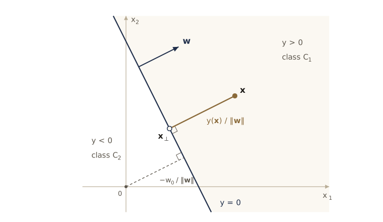
The next cell checks the three facts for the discriminant in the figure. The brute-force distance searches along the boundary line, which passes through \((0, 4)\) with direction \((1, -2)\).
w, w0 = np.array([2.0, 1.0]), -4.0
x = np.array([3.0, 2.5])

y_x = w @ x + w0
r = y_x / np.linalg.norm(w)                      # signed distance r = y(x)/||w||
x_perp = x - r * w / np.linalg.norm(w)           # foot of the perpendicular
print(f"y(x) = {y_x:.4f}   r = {r:.4f}   y(x_perp) = {w @ x_perp + w0:.4f}")

s = np.linspace(-10, 10, 200001)
line = np.array([0.0, 4.0]) + s[:, None] * np.array([1.0, -2.0])  # points with y = 0
d_search = np.linalg.norm(line - x, axis=1).min()
print(f"closest point on the line, by search: distance {d_search:.4f}")
print(f"w . (1, -2) = {w @ np.array([1.0, -2.0]):.1f}   "
      f"distance of boundary from origin: "
      f"{-w0 / np.linalg.norm(w):.4f}")
y(x) = 4.5000   r = 2.0125   y(x_perp) = 0.0000
closest point on the line, by search: distance 2.0125
w . (1, -2) = 0.0   distance of boundary from origin: 1.7889
A compact notation is often convenient: add a dummy input \(x_0 = 1\) and absorb the bias, writing \(\widetilde{\mathbf{w}} = (w_0, \mathbf{w})\) and \(\widetilde{\mathbf{x}} = (1, \mathbf{x})\), so that \(y(\mathbf{x}) = \widetilde{\mathbf{w}}^{\mathrm{T}}\widetilde{\mathbf{x}}\). In this augmented space of dimension \(D + 1\) every decision boundary passes through the origin. The helper add_bias builds \(\widetilde{\mathbf{x}}\).
Multiple classes
With \(K > 2\) classes it is tempting to reuse two-class discriminants, and there are two obvious ways.
A one-versus-the-rest classifier trains \(K\) (or \(K - 1\)) discriminants, the \(k\)th separating class \(\mathcal{C}_k\) from all the others. A one-versus-one classifier trains \(K(K-1)/2\) discriminants, one for every pair of classes, and lets them vote. Both leave parts of input space without a clear answer. In one-versus-the-rest, a point can be claimed by two classifiers or by none. In one-versus-one with three classes, the three pairwise boundaries generally do not pass through a single point; they enclose a small triangle, and inside it the votes go around in a circle — \(\mathcal{C}_1\) beats \(\mathcal{C}_2\), \(\mathcal{C}_2\) beats \(\mathcal{C}_3\), \(\mathcal{C}_3\) beats \(\mathcal{C}_1\) — so every class gets exactly one vote. We measure the one-versus-the-rest ambiguity on real data in the next section.
The cure is a single \(K\)-class discriminant made of \(K\) linear functions,
\[y_k(\mathbf{x}) = \mathbf{w}_k^{\mathrm{T}}\mathbf{x} + w_{k0}, \qquad k = 1, \dots, K,\]with the rule “assign \(\mathbf{x}\) to the class whose \(y_k(\mathbf{x})\) is largest”. Every point gets exactly one answer (up to exact ties, which have probability zero). The boundary between \(\mathcal{C}_k\) and \(\mathcal{C}_j\) is where \(y_k = y_j\), the hyperplane \((\mathbf{w}_k - \mathbf{w}_j)^{\mathrm{T}}\mathbf{x} + (w_{k0} - w_{j0}) = 0\), so the two-class geometry applies to every pair.
The decision regions of a \(K\)-class linear discriminant are always convex, so each one is a single connected piece. To see why, let \(\mathbf{x}_A\) and \(\mathbf{x}_B\) both lie in region \(\mathcal{R}_k\) and take any point between them, \(\widehat{\mathbf{x}} = \lambda \mathbf{x}_A + (1 - \lambda)\mathbf{x}_B\) with \(0 \le \lambda \le 1\). Each \(y_j\) is linear, so \(y_j(\widehat{\mathbf{x}}) = \lambda y_j(\mathbf{x}_A) + (1 - \lambda) y_j(\mathbf{x}_B)\). Since \(y_k\) beats every other \(y_j\) at both endpoints, it also beats it for the weighted average, and \(\widehat{\mathbf{x}}\) is in \(\mathcal{R}_k\) too.
For two classes, the \(K\)-class form with \(y_1\) and \(y_2\) is equivalent to the single discriminant \(y = y_1 - y_2\). We now look at three ways to learn the weights: least squares, Fisher’s criterion, and the perceptron.
Least squares for classification
In module 03, minimizing squared error gave a closed-form answer. Let us try the same thing with 1-of-\(K\) targets. Each class gets its own linear model, \(y_k(\mathbf{x}) = \widetilde{\mathbf{w}}_k^{\mathrm{T}}\widetilde{\mathbf{x}}\), and we collect the \(K\) weight vectors as the columns of a \((D+1) \times K\) matrix \(\widetilde{\mathbf{W}}\), so that \(\mathbf{y}(\mathbf{x}) = \widetilde{\mathbf{W}}^{\mathrm{T}}\widetilde{\mathbf{x}}\). With the augmented inputs as the rows of \(\widetilde{\mathbf{X}}\) and the targets as the rows of \(\mathbf{T}\), the sum-of-squares error over all outputs is
\[E_D(\widetilde{\mathbf{W}}) = \frac{1}{2} \operatorname{Tr}\left\{ (\widetilde{\mathbf{X}}\widetilde{\mathbf{W}} - \mathbf{T})^{\mathrm{T}} (\widetilde{\mathbf{X}}\widetilde{\mathbf{W}} - \mathbf{T}) \right\}.\]This is \(K\) separate regression problems sharing one design matrix. Its gradient with respect to \(\widetilde{\mathbf{W}}\) is \(\widetilde{\mathbf{X}}^{\mathrm{T}}(\widetilde{\mathbf{X}}\widetilde{\mathbf{W}} - \mathbf{T})\); setting it to zero gives the normal equations and
\[\widetilde{\mathbf{W}} = (\widetilde{\mathbf{X}}^{\mathrm{T}}\widetilde{\mathbf{X}})^{-1}\widetilde{\mathbf{X}}^{\mathrm{T}}\mathbf{T} = \widetilde{\mathbf{X}}^{\dagger}\mathbf{T},\]with \(\widetilde{\mathbf{X}}^{\dagger}\) the pseudo-inverse from module 03. As there, we compute it with lstsq rather than forming an inverse.
One justification: least squares estimates the conditional mean \(\mathbb{E}[\mathbf{t} \mid \mathbf{x}]\), and for 1-of-\(K\) targets that mean is exactly the vector of posterior class probabilities. So the outputs “want” to be probabilities. They even sum to one, because of a general property of least squares: if every training target satisfies the same linear constraint \(\mathbf{a}^{\mathrm{T}}\mathbf{t}_n + b = 0\), then so does the least-squares prediction at every input, \(\mathbf{a}^{\mathrm{T}}\mathbf{y}(\mathbf{x}) + b = 0\).
The proof is two lines. The constraint says \(\mathbf{T}\mathbf{a} = -b\,\mathbf{1}\). The vector \(\mathbf{1}\) is the first column of \(\widetilde{\mathbf{X}}\), so (with \(\widetilde{\mathbf{X}}\) of full column rank) \(\widetilde{\mathbf{X}}^{\dagger}\mathbf{1} = \mathbf{e}_1\), the first unit vector. Hence \(\widetilde{\mathbf{W}}\mathbf{a} = \widetilde{\mathbf{X}}^{\dagger}\mathbf{T}\mathbf{a} = -b\,\mathbf{e}_1\), and \(\mathbf{a}^{\mathrm{T}}\mathbf{y}(\mathbf{x}) = \widetilde{\mathbf{x}}^{\mathrm{T}}\widetilde{\mathbf{W}}\mathbf{a} = -b\) because the first entry of \(\widetilde{\mathbf{x}}\) is 1. With 1-of-\(K\) coding, \(\mathbf{a} = \mathbf{1}\) and \(b = -1\): the outputs always sum to one.
Summing to one is not enough to be a probability, though: nothing keeps the outputs inside \((0, 1)\). Our first data set has three classes in the plane whose means lie on a line, 50 points each.
def fit_least_squares(X, T):
    """W~ = pinv(X~) T, computed by least squares. Returns shape (D + 1, K)."""
    W, *_ = np.linalg.lstsq(add_bias(X), T, rcond=None)
    return W

def predict_argmax(W, X):
    return np.argmax(add_bias(X) @ W, axis=1)

rng3 = np.random.default_rng(30)
means3 = np.array([[-3.0, -3.0], [0.0, 0.0], [3.0, 3.0]])
X3 = np.vstack([rng3.normal(m, 1.0, size=(50, 2)) for m in means3])
lab3 = np.repeat(np.arange(3), 50)

W_ls3 = fit_least_squares(X3, one_hot(lab3, 3))
X_far = rng.normal(0.0, 10.0, size=(1000, 2))
Y_far = add_bias(X_far) @ W_ls3
print(f"outputs sum to one: max deviation {np.abs(Y_far.sum(axis=1) - 1).max():.1e}")
print(f"range of outputs on random points: [{Y_far.min():.2f}, {Y_far.max():.2f}]")
pred3 = predict_argmax(W_ls3, X3)
print(f"training errors: {np.sum(pred3 != lab3)} of {len(lab3)};"
      f"  points assigned to each class: {np.bincount(pred3, minlength=3)}")
outputs sum to one: max deviation 1.0e-14
range of outputs on random points: [-3.32, 4.77]
training errors: 31 of 150;  points assigned to each class: [66 21 63]
The outputs sum to one to machine precision, yet they range far outside \([0, 1]\). Worse, the classifier is bad on data that a linear classifier can handle easily: the middle class, which should get 50 points, is assigned only 21, and about a fifth of the training set is misclassified. This is called masking. The output for the middle class has to be a linear function of \(\mathbf{x}\) that is high in the middle and low at both ends, which no linear function can be, so it ends up nearly flat and wins the argmax only in a wedge off to the side of the data. The left panel of the figure below shows the result.
With the same data we can measure the ambiguity of one-versus-the-rest. We fit three two-class least-squares discriminants (targets \(+1\) for the class, \(-1\) for the rest) and count, on a grid of points covering the data, how many classifiers claim each point.
g = np.linspace(-7, 7, 141)
grid = np.array(np.meshgrid(g, g)).reshape(2, -1).T       # 141 x 141 points

claims = np.zeros((len(grid), 3), dtype=bool)
for k in range(3):
    t_k = np.where(lab3 == k, 1.0, -1.0)  # class k versus the rest
    w_k = fit_least_squares(X3, t_k)
    claims[:, k] = add_bias(grid) @ w_k > 0
n_claims = claims.sum(axis=1)
print(f"claimed by no class: {np.mean(n_claims == 0):.1%}   "
      f"by exactly one: {np.mean(n_claims == 1):.1%}   "
      f"by two or more: {np.mean(n_claims >= 2):.1%}")
claimed by no class: 5.7% by exactly one: 74.9% by two or more: 19.4%
A quarter of the plane gets no single answer. The \(K\)-class discriminant never has this problem; its trouble on this data set is the squared error, not the decision rule.
Least squares has a second weakness, which shows up even with two classes: it is not robust to outliers. The next cell fits two overlapping classes, then adds 20 extra points of class \(\mathcal{C}_2\) far away on the side where they already belong. A sensible classifier should not care: those points are correctly classified with a huge margin.
rng2 = np.random.default_rng(42)
X_a = rng2.normal([-1.0, 1.0], 1.0, size=(50, 2))           # class C1 (label 0)
X_b = rng2.normal([1.0, -1.0], 1.0, size=(50, 2))           # class C2 (label 1)
X_extra = rng2.normal([7.0, -4.0], 0.7, size=(20, 2))  # more C2, far on its own side
X2c = np.vstack([X_a, X_b])
lab2c = np.repeat([0, 1], 50)
X2o = np.vstack([X2c, X_extra])
lab2o = np.r_[lab2c, np.ones(20, dtype=int)]

def boundary_angle(v):
    """Direction of a 2-D weight vector (bias excluded), in degrees."""
    return np.degrees(np.arctan2(v[2], v[1]))

for name, X, lab in [("without outliers", X2c, lab2c),
                     ("with outliers   ", X2o, lab2o)]:
    W = fit_least_squares(X, one_hot(lab, 2))
    errs = np.sum(predict_argmax(W, X[:100]) != lab[:100])  # on the original 100
    print(f"{name}: errors on the original 100 points = {errs:2d},  "
          f"normal direction {boundary_angle(W[:, 0] - W[:, 1]):6.1f} deg")
without outliers: errors on the original 100 points =  3,  normal direction  132.6 deg
with outliers   : errors on the original 100 points =  9,  normal direction   98.8 deg
The 20 new points are all on the correct side, yet adding them rotates the boundary’s normal by about 34 degrees and triples the number of errors on the original points. Squared error penalizes a prediction of, say, \(y = -3\) for a point whose target is 0 just as much as a prediction of \(+3\): it punishes outputs that are “too correct”. The far-away points pull the fitted plane toward themselves to reduce those penalties, and the boundary moves.
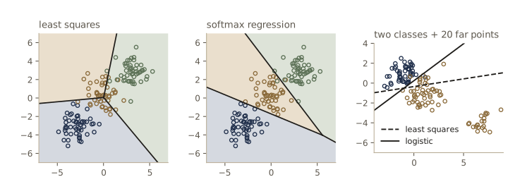
Both failures have the same root. Least squares is maximum likelihood under a Gaussian noise model (module 03), and a binary target is about as far from Gaussian as a variable can be. We come back to these data sets once we have logistic and softmax regression, which use a likelihood that fits the problem.
Watch out. A least-squares classifier is often fine on easy, balanced data, which makes it tempting. The failures above are not rare corner cases: any class sandwiched between others, and any cluster of confidently correct points, will distort it.
Fisher’s linear discriminant
Here is a different way to think about a two-class linear classifier. The quantity \(y = \mathbf{w}^{\mathrm{T}}\mathbf{x}\) projects the \(D\)-dimensional input onto a single line, and classifying is then a matter of placing a threshold on that line. Projecting throws information away, and classes that are well separated in \(D\) dimensions can overlap badly on a poorly chosen line. Fisher’s linear discriminant chooses the direction of projection to keep the classes apart.
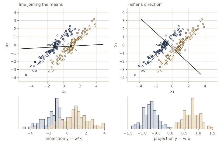
Let class \(\mathcal{C}_k\) have \(N_k\) points with mean \(\mathbf{m}_k\), so that the projected class means are \(m_k = \mathbf{w}^{\mathrm{T}}\mathbf{m}_k\). A first idea is to maximize the distance \(m_2 - m_1 = \mathbf{w}^{\mathrm{T}}(\mathbf{m}_2 - \mathbf{m}_1)\) between the projected means. This can be made as large as we like by scaling \(\mathbf{w}\), so we fix \(\lVert \mathbf{w} \rVert = 1\); a Lagrange multiplier (or the Cauchy–Schwarz inequality) then gives \(\mathbf{w} \propto \mathbf{m}_2 - \mathbf{m}_1\), the line joining the means.
That direction ignores the shape of the classes. If each class is a long, thin ellipse tilted relative to the line between the means, the projections spread out along the ellipse’s long axis and overlap. Fisher’s idea is to divide by the spread. Define the within-class variance of the projected class \(k\) as \(s_k^2 = \sum_{n \in \mathcal{C}_k} (y_n - m_k)^2\), with \(y_n = \mathbf{w}^{\mathrm{T}}\mathbf{x}_n\), and maximize the Fisher criterion
\[J(\mathbf{w}) = \frac{(m_2 - m_1)^2}{s_1^2 + s_2^2}.\]To see \(\mathbf{w}\) in it, write both parts as quadratic forms:
\[(m_2 - m_1)^2 = \mathbf{w}^{\mathrm{T}}(\mathbf{m}_2 - \mathbf{m}_1)(\mathbf{m}_2 - \mathbf{m}_1)^{\mathrm{T}}\mathbf{w}, \qquad s_k^2 = \sum_{n \in \mathcal{C}_k} \mathbf{w}^{\mathrm{T}}(\mathbf{x}_n - \mathbf{m}_k)(\mathbf{x}_n - \mathbf{m}_k)^{\mathrm{T}}\mathbf{w}.\]So
\[J(\mathbf{w}) = \frac{\mathbf{w}^{\mathrm{T}}\mathbf{S}_B\mathbf{w}}{\mathbf{w}^{\mathrm{T}}\mathbf{S}_W\mathbf{w}}, \qquad \mathbf{S}_B = (\mathbf{m}_2 - \mathbf{m}_1)(\mathbf{m}_2 - \mathbf{m}_1)^{\mathrm{T}}, \qquad \mathbf{S}_W = \sum_{k=1}^{2}\sum_{n \in \mathcal{C}_k} (\mathbf{x}_n - \mathbf{m}_k)(\mathbf{x}_n - \mathbf{m}_k)^{\mathrm{T}},\]where \(\mathbf{S}_B\) is the between-class covariance matrix and \(\mathbf{S}_W\) the within-class covariance matrix (both unnormalized “scatter” matrices). Now differentiate the ratio and set the gradient to zero. By the quotient rule, the gradient is proportional to \((\mathbf{w}^{\mathrm{T}}\mathbf{S}_W\mathbf{w})\mathbf{S}_B\mathbf{w} - (\mathbf{w}^{\mathrm{T}}\mathbf{S}_B\mathbf{w})\mathbf{S}_W\mathbf{w}\), so at the maximum
\[(\mathbf{w}^{\mathrm{T}}\mathbf{S}_B\mathbf{w})\,\mathbf{S}_W\mathbf{w} = (\mathbf{w}^{\mathrm{T}}\mathbf{S}_W\mathbf{w})\,\mathbf{S}_B\mathbf{w}.\]The two bracketed quantities are scalars. And \(\mathbf{S}_B\mathbf{w} = (\mathbf{m}_2 - \mathbf{m}_1)\left[(\mathbf{m}_2 - \mathbf{m}_1)^{\mathrm{T}}\mathbf{w}\right]\) always points along \(\mathbf{m}_2 - \mathbf{m}_1\). We only care about the direction of \(\mathbf{w}\), so dropping scalars and multiplying by \(\mathbf{S}_W^{-1}\) gives
Result. Fisher’s linear discriminant is the direction \(\mathbf{w} \propto \mathbf{S}_W^{-1}(\mathbf{m}_2 - \mathbf{m}_1)\).
If \(\mathbf{S}_W\) is a multiple of the identity (round classes), this reduces to the line joining the means. Otherwise \(\mathbf{S}_W^{-1}\) turns the direction away from the classes’ long axes. Strictly, Fisher’s result is a direction, not a classifier; to classify we still need a threshold \(y_0\) on the projected value. One reasonable choice is to fit a one-dimensional Gaussian to each projected class and use the decision theory of module 01; since \(y\) is a sum of many terms, the central limit theorem makes Gaussian projections a fair guess.
Our test data are two elongated classes with the same covariance, long axis along the diagonal. We compare the two directions by the criterion \(J\) and by the number of training errors made by the best possible threshold on the projection.
rngf = np.random.default_rng(7)
theta = np.pi / 4
Rot = np.array([[np.cos(theta), -np.sin(theta)], [np.sin(theta), np.cos(theta)]])
L_f = np.linalg.cholesky(Rot @ np.diag([4.0, 0.09]) @ Rot.T)   # long, thin, tilted
XF1 = rngf.normal(size=(100, 2)) @ L_f.T + np.array([-1.0, 0.0])
XF2 = rngf.normal(size=(100, 2)) @ L_f.T + np.array([1.0, 0.0])

def fisher_direction(X1, X2):
    """Unit vector along S_W^{-1} (m2 - m1)."""
    m1, m2 = X1.mean(axis=0), X2.mean(axis=0)
    S_W = (X1 - m1).T @ (X1 - m1) + (X2 - m2).T @ (X2 - m2)
    w = np.linalg.solve(S_W, m2 - m1)
    return w / np.linalg.norm(w)

def fisher_J(w, X1, X2):
    y1, y2 = X1 @ w, X2 @ w
    s2_within = np.sum((y1 - y1.mean())**2) + np.sum((y2 - y2.mean())**2)
    return (y2.mean() - y1.mean())**2 / s2_within

def best_threshold_errors(w, X1, X2):
    """Fewest training errors over all thresholds on the projection y = w^T x."""
    y = np.r_[X1 @ w, X2 @ w]
    is2 = np.r_[np.zeros(len(X1), bool), np.ones(len(X2), bool)][np.argsort(y)]
    # cut after the i-th smallest projection (i = 0..N); points below it -> class 1
    c2_below = np.r_[0, np.cumsum(is2)]  # class-2 points below the cut
    c1_below = np.r_[0, np.cumsum(~is2)]  # class-1 points below the cut
    errors = c2_below + (len(X1) - c1_below)            # C2 below + C1 above
    return int(min(errors.min(), (len(y) - errors).min()))   # either orientation

w_mean = XF2.mean(axis=0) - XF1.mean(axis=0)
w_mean /= np.linalg.norm(w_mean)
w_fish = fisher_direction(XF1, XF2)
for name, v in [("mean difference", w_mean), ("Fisher         ", w_fish)]:
    print(f"{name}: w = {v},  J = {fisher_J(v, XF1, XF2):.4f},  "
          f"best-threshold errors = {best_threshold_errors(v, XF1, XF2)} / 200")

angles = np.linspace(0, np.pi, 3601)  # brute force over all directions
J_all = [fisher_J(np.array([np.cos(a), np.sin(a)]), XF1, XF2) for a in angles]
print(f"largest J over a grid of 3601 directions: {max(J_all):.4f}")
mean difference: w = [0.9986 0.0538],  J = 0.0116,  best-threshold errors = 42 / 200
Fisher         : w = [ 0.7345 -0.6787],  J = 0.1431,  best-threshold errors = 0 / 200
largest J over a grid of 3601 directions: 0.1431
Projecting onto the line between the means leaves the classes heavily overlapped: even the best threshold misclassifies about a fifth of the points. Fisher’s direction, which is nearly perpendicular to the classes’ long axis, separates them perfectly, and its criterion value agrees with the best value found by brute force over all directions.
Relation to least squares
Least squares tried to hit target values; Fisher tried to separate projected classes. For two classes the two agree, provided we choose the targets cleverly: \(t_n = N/N_1\) for points of \(\mathcal{C}_1\) and \(t_n = -N/N_2\) for points of \(\mathcal{C}_2\), where \(N = N_1 + N_2\).
Minimize \(E = \frac{1}{2}\sum_n (\mathbf{w}^{\mathrm{T}}\mathbf{x}_n + w_0 - t_n)^2\). The condition \(\partial E/\partial w_0 = 0\) reads \(\sum_n (\mathbf{w}^{\mathrm{T}}\mathbf{x}_n + w_0 - t_n) = 0\). The targets were chosen so that \(\sum_n t_n = N_1 (N/N_1) - N_2 (N/N_2) = 0\), so
\[w_0 = -\mathbf{w}^{\mathrm{T}}\mathbf{m}, \qquad \mathbf{m} = \frac{1}{N}\sum_n \mathbf{x}_n,\]the bias puts the boundary through the overall mean. The condition \(\nabla_{\mathbf{w}}E = \mathbf{0}\), after substituting this \(w_0\), becomes
\[\sum_n \mathbf{x}_n (\mathbf{x}_n - \mathbf{m})^{\mathrm{T}}\mathbf{w} = \sum_n t_n \mathbf{x}_n = N(\mathbf{m}_1 - \mathbf{m}_2).\]On the left we may replace \(\mathbf{x}_n\) by \(\mathbf{x}_n - \mathbf{m}\), because \(\sum_n (\mathbf{x}_n - \mathbf{m}) = \mathbf{0}\); that turns the left side into \(\mathbf{S}_T\mathbf{w}\), where \(\mathbf{S}_T = \sum_n (\mathbf{x}_n - \mathbf{m})(\mathbf{x}_n - \mathbf{m})^{\mathrm{T}}\) is the total scatter. A little algebra (exercise 3) splits the total scatter into within-class and between-class parts, \(\mathbf{S}_T = \mathbf{S}_W + \frac{N_1 N_2}{N}\mathbf{S}_B\). So
\[\left(\mathbf{S}_W + \frac{N_1 N_2}{N}\mathbf{S}_B\right)\mathbf{w} = N(\mathbf{m}_1 - \mathbf{m}_2).\]Since \(\mathbf{S}_B\mathbf{w}\) points along \(\mathbf{m}_2 - \mathbf{m}_1\), we can move it to the right side: \(\mathbf{S}_W\mathbf{w} = c\,(\mathbf{m}_1 - \mathbf{m}_2)\) for a scalar \(c\), which one can show is positive. So \(\mathbf{w} \propto \mathbf{S}_W^{-1}(\mathbf{m}_1 - \mathbf{m}_2)\) — Fisher’s direction, pointing toward \(\mathcal{C}_1\) because \(\mathcal{C}_1\) has the positive targets — and the rule is: assign \(\mathbf{x}\) to \(\mathcal{C}_1\) when \(\mathbf{w}^{\mathrm{T}}(\mathbf{x} - \mathbf{m}) > 0\).
N1, N2 = len(XF1), len(XF2)
N = N1 + N2
XF = np.vstack([XF1, XF2])
t_fisher = np.r_[np.full(N1, N / N1), np.full(N2, -N / N2)]
w_tilde = fit_least_squares(XF, t_fisher)
w0_ls, w_ls = w_tilde[0], w_tilde[1:]
cos = w_ls @ -w_fish / np.linalg.norm(w_ls)
print(f"cosine between least-squares w and S_W^-1 (m1 - m2): {cos:.6f}")
print(f"w0 = {w0_ls:.6f}   -w^T m = {-w_ls @ XF.mean(axis=0):.6f}")

m1, m2, m = XF1.mean(axis=0), XF2.mean(axis=0), XF.mean(axis=0)
S_W = (XF1 - m1).T @ (XF1 - m1) + (XF2 - m2).T @ (XF2 - m2)
S_T = (XF - m).T @ (XF - m)
S_B = np.outer(m2 - m1, m2 - m1)
err = np.abs(S_T - S_W - N1 * N2 / N * S_B).max()
print(f"S_T = S_W + (N1 N2 / N) S_B: max error {err:.1e}")
cosine between least-squares w and S_W^-1 (m1 - m2): 1.000000
w0 = 0.033759   -w^T m = 0.033759
S_T = S_W + (N1 N2 / N) S_B: max error 1.1e-13
The least-squares weight vector is parallel to Fisher’s direction to six decimal places, and its bias is exactly \(-\mathbf{w}^{\mathrm{T}}\mathbf{m}\).
Fisher’s discriminant for multiple classes
With \(K > 2\) classes and inputs of dimension \(D > K\), we can look for \(D' > 1\) projections at once, \(\mathbf{y} = \mathbf{W}^{\mathrm{T}}\mathbf{x}\), where the columns of the \(D \times D'\) matrix \(\mathbf{W}\) are the projection directions. The within-class scatter \(\mathbf{S}_W\) generalizes directly, as a sum of the \(K\) class scatter matrices. For the between-class scatter, start from the total scatter \(\mathbf{S}_T\) about the overall mean \(\mathbf{m}\) and subtract the within-class part. The two matrices are
\[\mathbf{S}_W = \sum_{k=1}^{K} \sum_{n \in \mathcal{C}_k} (\mathbf{x}_n - \mathbf{m}_k)(\mathbf{x}_n - \mathbf{m}_k)^{\mathrm{T}}, \qquad \mathbf{S}_B = \mathbf{S}_T - \mathbf{S}_W = \sum_{k=1}^{K} N_k (\mathbf{m}_k - \mathbf{m})(\mathbf{m}_k - \mathbf{m})^{\mathrm{T}}.\]A natural criterion is
\[J(\mathbf{W}) = \operatorname{Tr}\left\{(\mathbf{W}^{\mathrm{T}}\mathbf{S}_W\mathbf{W})^{-1}(\mathbf{W}^{\mathrm{T}}\mathbf{S}_B\mathbf{W})\right\},\]large when the projected class means are spread out relative to the projected spread within classes. It is maximized by taking as columns of \(\mathbf{W}\) the eigenvectors of \(\mathbf{S}_W^{-1}\mathbf{S}_B\) with the largest eigenvalues (Bishop §4.1.6 points to the literature for the derivation; several other criteria lead to the same eigenproblem).
There is a hard limit on how many useful directions exist. \(\mathbf{S}_B\) is a sum of \(K\) rank-one matrices, and they are not independent: \(\sum_k N_k(\mathbf{m}_k - \mathbf{m}) = \mathbf{0}\). So \(\mathbf{S}_B\) has rank at most \(K - 1\), and at most \(K - 1\) eigenvalues of \(\mathbf{S}_W^{-1}\mathbf{S}_B\) are nonzero. Fisher’s method can find at most \(K - 1\) discriminating features, however large \(D\) is.
rngm = np.random.default_rng(11)
K4, D4 = 3, 5
class_means = rngm.normal(0, 2, size=(K4, D4))
Xm = np.vstack([rngm.normal(class_means[k], 1.0, size=(40, D4)) for k in range(K4)])
labm = np.repeat(np.arange(K4), 40)
mm = Xm.mean(axis=0)
S_Wm, S_Bm = np.zeros((D4, D4)), np.zeros((D4, D4))
for k in range(K4):
    Xk = Xm[labm == k]
    mk = Xk.mean(axis=0)
    S_Wm += (Xk - mk).T @ (Xk - mk)                        # within-class scatter
    S_Bm += len(Xk) * np.outer(mk - mm, mk - mm)          # between-class scatter
eig = np.sort(np.linalg.eigvals(np.linalg.solve(S_Wm, S_Bm)).real)[::-1]
print(f"eigenvalues of S_W^-1 S_B (K = {K4}, D = {D4}): {eig}")
eigenvalues of S_W^-1 S_B (K = 3, D = 5): [ 7.3831 2.5957 0. 0. -0. ]
Two eigenvalues are clearly nonzero and the other three vanish to rounding error, exactly \(K - 1 = 2\) useful directions in five dimensions.
The perceptron algorithm
The perceptron is a two-class linear discriminant with a step activation. It uses targets \(t \in \{-1, +1\}\) and outputs
\[y(\mathbf{x}) = f\left(\mathbf{w}^{\mathrm{T}}\boldsymbol{\phi}(\mathbf{x})\right), \qquad f(a) = \begin{cases} +1, & a \ge 0 \\ -1, & a < 0, \end{cases}\]where the feature vector \(\boldsymbol{\phi}\) includes a constant \(\phi_0 = 1\) for the bias. A point is correctly classified when \(\mathbf{w}^{\mathrm{T}}\boldsymbol{\phi}_n t_n > 0\).
The obvious error function, the number of misclassified points, is piecewise constant in \(\mathbf{w}\): its gradient is zero almost everywhere, so it gives gradient methods nothing to follow. The perceptron criterion replaces it with a quantity that grows the further a mistake is from being corrected:
\[E_P(\mathbf{w}) = -\sum_{n \in \mathcal{M}} \mathbf{w}^{\mathrm{T}}\boldsymbol{\phi}_n t_n ,\]where \(\mathcal{M}\) is the set of misclassified points. Each term is nonnegative (a misclassified point has \(\mathbf{w}^{\mathrm{T}}\boldsymbol{\phi}_n t_n \le 0\)), correct points contribute nothing, and within any region of weight space where the set of mistakes is fixed, \(E_P\) is linear in \(\mathbf{w}\). Stochastic gradient descent on one misclassified point at a time gives the perceptron learning rule
\[\mathbf{w}^{(\tau+1)} = \mathbf{w}^{(\tau)} + \eta\,\boldsymbol{\phi}_n t_n .\]The classifier does not change when \(\mathbf{w}\) is scaled, so the learning rate can be set to \(\eta = 1\). In words: cycle through the data; when a point is misclassified, add its feature vector to \(\mathbf{w}\) if it is in \(\mathcal{C}_1\) and subtract it if it is in \(\mathcal{C}_2\). One update always reduces the error on the point that triggered it — its term \(-\mathbf{w}^{\mathrm{T}}\boldsymbol{\phi}_n t_n\) drops by \(\lVert \boldsymbol{\phi}_n \rVert^2\) — but it can break points that were correct. So \(E_P\) need not decrease at every step. On separable data, though, the algorithm is guaranteed to stop.
Result (perceptron convergence). Suppose some unit vector \(\mathbf{u}\) separates the data with margin \(\gamma > 0\), meaning \(t_n\mathbf{u}^{\mathrm{T}}\boldsymbol{\phi}_n \ge \gamma\) for every \(n\), and let \(R = \max_n \lVert \boldsymbol{\phi}_n \rVert\). Starting from \(\mathbf{w} = \mathbf{0}\), the perceptron makes at most \((R/\gamma)^2\) updates.
The proof follows two quantities through the updates. Let \(\mathbf{w}_k\) be the weight vector after \(k\) updates.
- Progress along \(\mathbf{u}\). Each update adds \(t_n\boldsymbol{\phi}_n\), so \(\mathbf{u}^{\mathrm{T}}\mathbf{w}_k\) grows by \(t_n\mathbf{u}^{\mathrm{T}}\boldsymbol{\phi}_n \ge \gamma\). After \(k\) updates, \(\mathbf{u}^{\mathrm{T}}\mathbf{w}_k \ge k\gamma\).
- Slow growth of the length. Expanding the square, the update changes \(\lVert \mathbf{w} \rVert^2\) by \(2t_n\mathbf{w}_{k-1}^{\mathrm{T}}\boldsymbol{\phi}_n + \lVert \boldsymbol{\phi}_n \rVert^2\). The first part is at most zero, because updates happen only on mistakes, and the second is at most \(R^2\). So \(\lVert \mathbf{w}_k \rVert^2 \le kR^2\).
Since \(\mathbf{u}\) is a unit vector, \(\mathbf{u}^{\mathrm{T}}\mathbf{w}_k \le \lVert \mathbf{w}_k \rVert\), so \(k\gamma \le \sqrt{k}\,R\), which gives \(k \le (R/\gamma)^2\). The bound depends on the geometry of the data, not on the number of points.
We test this on 200 points in a square, labeled by a known line and kept only if they are at least 0.05 from it, so that the true line separates them with a small margin.
def perceptron(Phi, t, max_epochs=1000, rng=None):
    """Perceptron learning rule. Returns (w, updates, epochs used, converged)."""
    w = np.zeros(Phi.shape[1])
    updates = 0
    for epoch in range(1, max_epochs + 1):
        order = rng.permutation(len(t)) if rng is not None else range(len(t))
        mistakes = 0
        for n in order:
            if t[n] * (w @ Phi[n]) <= 0:  # misclassified (or on the boundary)
                w = w + t[n] * Phi[n]             # w <- w + phi_n t_n
                updates += 1
                mistakes += 1
        if mistakes == 0:
            return w, updates, epoch, True
    return w, updates, max_epochs, False

rngp = np.random.default_rng(3)
w_true = np.array([-0.5, 1.0, 2.0])                       # (bias, w1, w2)
Xp = rngp.uniform(-3, 3, size=(2000, 2))
dist = add_bias(Xp) @ w_true / np.linalg.norm(w_true[1:])  # distance to true line
Xp = Xp[np.abs(dist) > 0.05][:200]
Phi_p = add_bias(Xp)
t_p = np.sign(Phi_p @ w_true)

w_hat, updates, epochs, ok = perceptron(Phi_p, t_p)
print(f"converged: {ok} after {updates} updates ({epochs} passes); "
      f"training errors {np.sum(np.sign(Phi_p @ w_hat) != t_p)}")
u = w_true / np.linalg.norm(w_true)  # a separating unit vector
gamma = np.min(t_p * (Phi_p @ u))
R = np.max(np.linalg.norm(Phi_p, axis=1))
print(f"R = {R:.3f}, gamma = {gamma:.4f}, bound (R/gamma)^2 = {(R / gamma)**2:.0f}")
rng_order = np.random.default_rng(0)
counts = [perceptron(Phi_p, t_p, rng=rng_order)[1] for _ in range(20)]
print(f"updates over 20 random orders: min {min(counts)}, "
      f"median {int(np.median(counts))}, max {max(counts)}")
converged: True after 35 updates (7 passes); training errors 0
R = 4.245, gamma = 0.0547, bound (R/gamma)^2 = 6020
updates over 20 random orders: min 5, median 26, max 51
The perceptron stops after a few dozen updates, while the bound allows about 6,000: it is a worst case over every data set with the same \(R\) and \(\gamma\) (and \(\gamma\) here is measured for the true line, not for the best separator). Different presentation orders give different numbers of updates and different final lines — any separating line stops the algorithm, and which one we get depends on the order and the start.
On data that are not separable the perceptron never settles. On the overlapping two-class data from the least-squares section, the number of mistakes per pass keeps bouncing around:
t_c = np.where(lab2c == 0, 1.0, -1.0)
w_c = np.zeros(3)
per_pass = []
for epoch in range(50):
    mistakes = 0
    for n in range(len(t_c)):
        if t_c[n] * (w_c @ add_bias(X2c)[n]) <= 0:
            w_c = w_c + t_c[n] * add_bias(X2c)[n]
            mistakes += 1
    per_pass.append(mistakes)
print("mistakes in passes 1-10: ", per_pass[:10])
print("mistakes in passes 41-50:", per_pass[40:])
mistakes in passes 1-10:  [4, 7, 6, 6, 6, 7, 4, 4, 4, 4]
mistakes in passes 41-50: [4, 4, 4, 4, 6, 7, 8, 6, 6, 8]
The perceptron has further limitations: its output is a hard label with no probability, it does not extend naturally to more than two classes, and on data that are not separable it gives no signal that it will never converge — a slow problem and an impossible one look the same while it runs. A related early model, the adaline, used the same linear model but trained it by minimizing squared error, the method of the least-squares section. What the perceptron shares with every model in this module is the most important limitation of all: the features \(\boldsymbol{\phi}\) are fixed. Learning the features is the subject of module 05.
Probabilistic generative models
We now turn to probabilistic models, starting with the generative approach: model each class-conditional density \(p(\mathbf{x} \mid \mathcal{C}_k)\) and the priors \(p(\mathcal{C}_k)\), and get posteriors from Bayes’ theorem. For two classes,
\[p(\mathcal{C}_1 \mid \mathbf{x}) = \frac{p(\mathbf{x} \mid \mathcal{C}_1)p(\mathcal{C}_1)}{p(\mathbf{x} \mid \mathcal{C}_1)p(\mathcal{C}_1) + p(\mathbf{x} \mid \mathcal{C}_2)p(\mathcal{C}_2)} = \frac{1}{1 + \exp(-a)} = \sigma(a), \qquad a = \ln\frac{p(\mathbf{x} \mid \mathcal{C}_1)p(\mathcal{C}_1)}{p(\mathbf{x} \mid \mathcal{C}_2)p(\mathcal{C}_2)}.\](Divide the numerator and denominator by the numerator.) Here \(\sigma\) is the logistic sigmoid, an S-shaped function that squashes the real line into \((0, 1)\). The quantity \(a\) is the log odds, \(a = \ln\left[p(\mathcal{C}_1 \mid \mathbf{x}) / p(\mathcal{C}_2 \mid \mathbf{x})\right]\), and the inverse of the sigmoid, \(a = \ln\left[\sigma / (1 - \sigma)\right]\), is called the logit function. The sigmoid has two properties we use repeatedly:
\[\sigma(-a) = 1 - \sigma(a), \qquad \frac{d\sigma}{da} = \sigma(a)\left(1 - \sigma(a)\right).\]Rewriting the posterior this way looks like a triviality — any posterior can be written as \(\sigma(a)\). It becomes useful when \(a(\mathbf{x})\) has a simple form, and we will see that under common assumptions it is linear in \(\mathbf{x}\).
For \(K\) classes the same manipulation gives
\[p(\mathcal{C}_k \mid \mathbf{x}) = \frac{\exp(a_k)}{\sum_j \exp(a_j)}, \qquad a_k = \ln p(\mathbf{x} \mid \mathcal{C}_k)p(\mathcal{C}_k),\]the normalized exponential or softmax function. It is a smooth version of “max”: if one \(a_k\) is much larger than the rest, its probability is close to 1 and the others close to 0. For \(K = 2\), softmax reduces to the sigmoid of \(a_1 - a_2\).
In code, scipy.special.expit is a numerically safe sigmoid, and softmax must subtract the largest activation (or use log-sum-exp) to avoid overflow.
def softmax(A):
    """Softmax along the last axis, via log-sum-exp (no overflow for large inputs)."""
    return np.exp(A - logsumexp(A, axis=-1, keepdims=True))

a = np.linspace(-8, 8, 17)
s = expit(a)
h = 1e-6
ds_num = (expit(a + h) - expit(a - h)) / (2 * h)
print(f"sigma(-a) = 1 - sigma(a): max error {np.abs(expit(-a) - (1 - s)).max():.1e}")
logit = np.log(s / (1 - s))
print(f"logit(sigma(a)) = a:      max error {np.abs(logit - a).max():.1e}")
print(f"d sigma/da = s(1 - s):    max error {np.abs(ds_num - s * (1 - s)).max():.1e}")
print("softmax([1000, 1001, 999]) =", softmax(np.array([1000.0, 1001.0, 999.0])))
p2 = softmax(np.array([2.0, -1.0]))[0]
print(f"two-class softmax {p2:.6f} = sigmoid(3) {expit(3.0):.6f}")
sigma(-a) = 1 - sigma(a): max error 1.5e-16
logit(sigma(a)) = a:      max error 3.2e-13
d sigma/da = s(1 - s):    max error 7.2e-11
softmax([1000, 1001, 999]) = [0.2447 0.6652 0.09  ]
two-class softmax 0.952574 = sigmoid(3) 0.952574
Continuous inputs
Suppose the class-conditional densities are Gaussian and, for now, share one covariance matrix:
\[p(\mathbf{x} \mid \mathcal{C}_k) = \mathcal{N}(\mathbf{x} \mid \boldsymbol{\mu}_k, \boldsymbol{\Sigma}) = \frac{1}{(2\pi)^{D/2}\lvert \boldsymbol{\Sigma} \rvert^{1/2}} \exp\left\{-\frac{1}{2}(\mathbf{x} - \boldsymbol{\mu}_k)^{\mathrm{T}}\boldsymbol{\Sigma}^{-1}(\mathbf{x} - \boldsymbol{\mu}_k)\right\}.\]Compute the log odds for two classes. The normalizing constants are equal and cancel. Expanding the quadratic forms,
\[\begin{aligned} a &= -\frac{1}{2}(\mathbf{x} - \boldsymbol{\mu}_1)^{\mathrm{T}}\boldsymbol{\Sigma}^{-1}(\mathbf{x} - \boldsymbol{\mu}_1) + \frac{1}{2}(\mathbf{x} - \boldsymbol{\mu}_2)^{\mathrm{T}}\boldsymbol{\Sigma}^{-1}(\mathbf{x} - \boldsymbol{\mu}_2) + \ln\frac{p(\mathcal{C}_1)}{p(\mathcal{C}_2)} \\ &= (\boldsymbol{\mu}_1 - \boldsymbol{\mu}_2)^{\mathrm{T}}\boldsymbol{\Sigma}^{-1}\mathbf{x} - \frac{1}{2}\boldsymbol{\mu}_1^{\mathrm{T}}\boldsymbol{\Sigma}^{-1}\boldsymbol{\mu}_1 + \frac{1}{2}\boldsymbol{\mu}_2^{\mathrm{T}}\boldsymbol{\Sigma}^{-1}\boldsymbol{\mu}_2 + \ln\frac{p(\mathcal{C}_1)}{p(\mathcal{C}_2)}, \end{aligned}\]because the two copies of \(\mathbf{x}^{\mathrm{T}}\boldsymbol{\Sigma}^{-1}\mathbf{x}\) cancel (this is where the shared covariance matters) and the cross terms combine using the symmetry of \(\boldsymbol{\Sigma}^{-1}\). So with Gaussian class-conditionals sharing a covariance, \(p(\mathcal{C}_1 \mid \mathbf{x}) = \sigma(\mathbf{w}^{\mathrm{T}}\mathbf{x} + w_0)\) with
\[\mathbf{w} = \boldsymbol{\Sigma}^{-1}(\boldsymbol{\mu}_1 - \boldsymbol{\mu}_2), \qquad w_0 = -\frac{1}{2}\boldsymbol{\mu}_1^{\mathrm{T}}\boldsymbol{\Sigma}^{-1}\boldsymbol{\mu}_1 + \frac{1}{2}\boldsymbol{\mu}_2^{\mathrm{T}}\boldsymbol{\Sigma}^{-1}\boldsymbol{\mu}_2 + \ln\frac{p(\mathcal{C}_1)}{p(\mathcal{C}_2)}.\]The posterior is a generalized linear model, the decision boundary (where the posterior is one half, \(a = 0\)) is a hyperplane, and so is every contour of constant posterior probability. The priors enter only through \(w_0\): changing them slides these hyperplanes parallel to themselves. Compare \(\mathbf{w}\) with Fisher’s direction \(\mathbf{S}_W^{-1}(\mathbf{m}_2 - \mathbf{m}_1)\): up to sign and scale, it is the same formula with population quantities in place of sample ones.
For \(K\) classes, \(a_k(\mathbf{x}) = \mathbf{w}_k^{\mathrm{T}}\mathbf{x} + w_{k0}\) with \(\mathbf{w}_k = \boldsymbol{\Sigma}^{-1}\boldsymbol{\mu}_k\) and \(w_{k0} = -\frac{1}{2}\boldsymbol{\mu}_k^{\mathrm{T}}\boldsymbol{\Sigma}^{-1}\boldsymbol{\mu}_k + \ln p(\mathcal{C}_k)\), after dropping the term \(-\frac{1}{2}\mathbf{x}^{\mathrm{T}}\boldsymbol{\Sigma}^{-1}\mathbf{x}\) that is common to all classes and cancels in the softmax. Again the boundaries are linear. This model is often called linear discriminant analysis.
If each class has its own covariance \(\boldsymbol{\Sigma}_k\), the quadratic terms no longer cancel:
\[a_k(\mathbf{x}) = -\frac{1}{2}(\mathbf{x} - \boldsymbol{\mu}_k)^{\mathrm{T}}\boldsymbol{\Sigma}_k^{-1}(\mathbf{x} - \boldsymbol{\mu}_k) - \frac{1}{2}\ln\lvert \boldsymbol{\Sigma}_k \rvert + \ln p(\mathcal{C}_k) + \text{const},\]and the decision boundaries are quadratic surfaces: quadratic discriminant analysis. When some pairs of classes share a covariance and others don’t, the boundaries between the sharing pairs are still linear.
We need the Gaussian log density; here is a Cholesky-based version, checked against scipy.stats.
def gauss_logpdf(X, mu, Sigma):
    """ln N(x | mu, Sigma) for each row of X, via the Cholesky factor of Sigma."""
    L = np.linalg.cholesky(Sigma)
    Z = np.linalg.solve(L, (X - mu).T)                 # whitened residuals
    D = len(mu)
    log_det_half = np.sum(np.log(np.diag(L)))           # (1/2) ln |Sigma|
    return -0.5 * np.sum(Z**2, axis=0) - log_det_half - 0.5 * D * np.log(2 * np.pi)

Xt = rng.normal(size=(5, 2))
mu_t, Sig_t = np.array([0.5, -1.0]), np.array([[2.0, 0.6], [0.6, 1.0]])
ref = stats.multivariate_normal(mu_t, Sig_t).logpdf(Xt)
err = np.abs(gauss_logpdf(Xt, mu_t, Sig_t) - ref).max()
print(f"max difference from scipy.stats: {err:.1e}")
max difference from scipy.stats: 3.6e-15
Maximum likelihood solution
To use these models we need \(\boldsymbol{\mu}_k\), \(\boldsymbol{\Sigma}\), and the priors. Given labeled data, we fit them by maximum likelihood. Take two classes, write \(p(\mathcal{C}_1) = \pi\), and code \(t_n = 1\) for \(\mathcal{C}_1\) and \(t_n = 0\) for \(\mathcal{C}_2\). A point from \(\mathcal{C}_1\) contributes \(p(\mathbf{x}_n, \mathcal{C}_1) = \pi\,\mathcal{N}(\mathbf{x}_n \mid \boldsymbol{\mu}_1, \boldsymbol{\Sigma})\) and a point from \(\mathcal{C}_2\) contributes \((1 - \pi)\,\mathcal{N}(\mathbf{x}_n \mid \boldsymbol{\mu}_2, \boldsymbol{\Sigma})\), so the likelihood of the labeled data is
\[p(\mathbf{t}, \mathbf{X} \mid \pi, \boldsymbol{\mu}_1, \boldsymbol{\mu}_2, \boldsymbol{\Sigma}) = \prod_{n=1}^{N} \left[\pi\,\mathcal{N}(\mathbf{x}_n \mid \boldsymbol{\mu}_1, \boldsymbol{\Sigma})\right]^{t_n} \left[(1 - \pi)\,\mathcal{N}(\mathbf{x}_n \mid \boldsymbol{\mu}_2, \boldsymbol{\Sigma})\right]^{1 - t_n}.\]The log likelihood splits into separate pieces for each parameter.
The prior. The terms involving \(\pi\) are \(\sum_n \{t_n \ln \pi + (1 - t_n)\ln(1 - \pi)\}\). Setting the derivative \(N_1/\pi - N_2/(1 - \pi)\) to zero gives \(\pi = N_1/N\), the fraction of training points in \(\mathcal{C}_1\). With \(K\) classes (and a Lagrange multiplier for \(\sum_k \pi_k = 1\)) the answer is again \(\pi_k = N_k/N\).
The means. The terms involving \(\boldsymbol{\mu}_1\) are \(-\frac{1}{2}\sum_n t_n(\mathbf{x}_n - \boldsymbol{\mu}_1)^{\mathrm{T}}\boldsymbol{\Sigma}^{-1}(\mathbf{x}_n - \boldsymbol{\mu}_1)\). The gradient is \(\boldsymbol{\Sigma}^{-1}\sum_n t_n(\mathbf{x}_n - \boldsymbol{\mu}_1)\), which vanishes at \(\boldsymbol{\mu}_1 = \frac{1}{N_1}\sum_n t_n\mathbf{x}_n\), the sample mean of class \(\mathcal{C}_1\). Likewise \(\boldsymbol{\mu}_2\) is the mean of class \(\mathcal{C}_2\).
The shared covariance. Collecting the terms that involve \(\boldsymbol{\Sigma}\) from both classes,
\[-\frac{N}{2}\ln\lvert \boldsymbol{\Sigma} \rvert - \frac{1}{2}\sum_{k=1}^{2}\sum_{n \in \mathcal{C}_k}(\mathbf{x}_n - \boldsymbol{\mu}_k)^{\mathrm{T}}\boldsymbol{\Sigma}^{-1}(\mathbf{x}_n - \boldsymbol{\mu}_k) = -\frac{N}{2}\ln\lvert \boldsymbol{\Sigma} \rvert - \frac{N}{2}\operatorname{Tr}\left(\boldsymbol{\Sigma}^{-1}\mathbf{S}\right),\]where we used \(\mathbf{a}^{\mathrm{T}}\mathbf{B}\mathbf{a} = \operatorname{Tr}(\mathbf{B}\mathbf{a}\mathbf{a}^{\mathrm{T}})\) and defined
\[\mathbf{S} = \frac{N_1}{N}\mathbf{S}_1 + \frac{N_2}{N}\mathbf{S}_2, \qquad \mathbf{S}_k = \frac{1}{N_k}\sum_{n \in \mathcal{C}_k}(\mathbf{x}_n - \boldsymbol{\mu}_k)(\mathbf{x}_n - \boldsymbol{\mu}_k)^{\mathrm{T}}.\]This has exactly the form of the log likelihood of a single Gaussian with sample covariance \(\mathbf{S}\), whose maximizer we found in module 02: \(\boldsymbol{\Sigma} = \mathbf{S}\). The shared covariance is the average of the per-class covariances, weighted by class size. With separate covariances, each \(\boldsymbol{\Sigma}_k = \mathbf{S}_k\).
def fit_gaussian_classes(X, labels, K, shared=True):
    """ML priors, means, and covariances (shared or per class) of Gaussian classes."""
    N = len(X)
    priors = np.bincount(labels, minlength=K) / N                   # pi_k = N_k / N
    means = np.array([X[labels == k].mean(axis=0) for k in range(K)])
    covs = np.array([np.cov(X[labels == k].T, bias=True)  # S_k (divide by N_k)
                     for k in range(K)])
    if shared:
        S = np.einsum("k,kij->ij", priors, covs)  # sum_k (N_k/N) S_k
        covs = np.array([S] * K)
    return priors, means, covs

def gaussian_log_joint(X, model):
    """a_k(x) = ln p(x | C_k) + ln p(C_k), shape (N, K)."""
    priors, means, covs = model
    return np.column_stack([gauss_logpdf(X, means[k], covs[k]) + np.log(priors[k])
                            for k in range(len(priors))])

def gaussian_posterior(X, model):
    return softmax(gaussian_log_joint(X, model))

def gaussian_log_likelihood(X, labels, model):
    return np.sum(gaussian_log_joint(X, model)[np.arange(len(X)), labels])
We test the linear form on the elongated two-class data from the Fisher section, where the two classes really do share a covariance. We also check that the fitted covariance is a maximum by nudging it in random symmetric directions.
labF = np.repeat([0, 1], 100)
model_F = fit_gaussian_classes(XF, labF, 2, shared=True)
pri, mus, covs = model_F
Sigma = covs[0]
w_gen = np.linalg.solve(Sigma, mus[0] - mus[1])  # Sigma^-1 (mu1 - mu2)
w0_gen = (-0.5 * mus[0] @ np.linalg.solve(Sigma, mus[0])
          + 0.5 * mus[1] @ np.linalg.solve(Sigma, mus[1]) + np.log(pri[0] / pri[1]))
P = gaussian_posterior(XF, model_F)
err = np.abs(P[:, 0] - expit(XF @ w_gen + w0_gen)).max()
print(f"p(C1|x) from Bayes vs sigmoid(w^T x + w0): max difference {err:.1e}")
cos = w_gen @ -w_fish / np.linalg.norm(w_gen)
print(f"cosine between w and Fisher's direction: {cos:.6f}")

ll_best = gaussian_log_likelihood(XF, labF, model_F)
worse = 0
for _ in range(200):
    B = rng.normal(size=(2, 2)) * 0.02
    Sig_try = Sigma + (B + B.T) / 2
    ll_try = gaussian_log_likelihood(XF, labF, (pri, mus, np.array([Sig_try] * 2)))
    worse += ll_try < ll_best
print(f"random perturbations of Sigma that lower the log likelihood: {worse} of 200")
p(C1|x) from Bayes vs sigmoid(w^T x + w0): max difference 7.2e-16
cosine between w and Fisher's direction: 1.000000
random perturbations of Sigma that lower the log likelihood: 200 of 200
The Bayes posterior and the sigmoid of the linear function agree to rounding error, and the generative weight vector points exactly along Fisher’s direction (the sign flips because \(\mathbf{w}\) points toward \(\mathcal{C}_1\)). Every perturbation of the fitted covariance lowers the likelihood.
Now data where the shared-covariance assumption is wrong: a broad, tilted class and a compact one. We fit both models on 200 points and evaluate them on 10,000 fresh points from the same distribution.
def sample_two_shapes(rng, n):
    means = [np.array([0.0, 0.0]), np.array([1.5, 1.0])]
    covs = [np.array([[4.0, 1.2], [1.2, 1.5]]), np.array([[0.3, -0.1], [-0.1, 0.25]])]
    X = np.vstack([rng.multivariate_normal(means[k], covs[k], n) for k in range(2)])
    return X, np.repeat([0, 1], n)

rngq = np.random.default_rng(12)
Xq, labq = sample_two_shapes(rngq, 100)
Xq_test, labq_test = sample_two_shapes(rngq, 5000)
for name, shared in [("shared covariance (linear)   ", True),
                     ("separate covariances (quad.)", False)]:
    model = fit_gaussian_classes(Xq, labq, 2, shared=shared)
    err_tr = np.mean(gaussian_posterior(Xq, model).argmax(axis=1) != labq)
    err_te = np.mean(gaussian_posterior(Xq_test, model).argmax(axis=1) != labq_test)
    print(f"{name}: training error {err_tr:.1%}, test error {err_te:.1%}")
shared covariance (linear)   : training error 16.5%, test error 17.8%
separate covariances (quad.): training error 11.5%, test error 11.7%
The quadratic boundary curls around the compact class and cuts the test error by about a third.
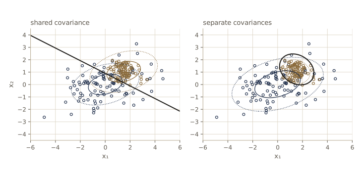
The price of the quadratic model is parameters: each class now has its own \(D(D+1)/2\) covariance entries, which is fine in two dimensions and hopeless in hundreds. Also, fitting Gaussians by maximum likelihood inherits the Gaussian’s sensitivity to outliers (module 02): a few wild points can change a class’s mean and covariance a lot.
Discrete features
Now suppose the inputs are \(D\) binary features, \(x_i \in \{0, 1\}\) — words present or absent in a document, say. A fully general class-conditional distribution would be a table with \(2^D - 1\) free entries per class, which is impossible to estimate for even moderate \(D\). The naive Bayes assumption cuts this down: within each class, the features are treated as independent,
\[p(\mathbf{x} \mid \mathcal{C}_k) = \prod_{i=1}^{D} \mu_{ki}^{x_i}(1 - \mu_{ki})^{1 - x_i},\]where \(\mu_{ki}\) is the probability that feature \(i\) is on in class \(k\). That is \(D\) parameters per class. (The assumption is rarely true; the name admits it. Module 08 will describe it as a graphical model.) Substituting into \(a_k = \ln p(\mathbf{x} \mid \mathcal{C}_k)p(\mathcal{C}_k)\) gives
\[a_k(\mathbf{x}) = \sum_{i=1}^{D}\left\{x_i\ln\mu_{ki} + (1 - x_i)\ln(1 - \mu_{ki})\right\} + \ln p(\mathcal{C}_k),\]which is again linear in the inputs. For two classes the log odds is \(a = \mathbf{w}^{\mathrm{T}}\mathbf{x} + w_0\) with \(w_i = \ln\frac{\mu_{1i}}{\mu_{2i}} - \ln\frac{1 - \mu_{1i}}{1 - \mu_{2i}}\) and \(w_0 = \sum_i \ln\frac{1 - \mu_{1i}}{1 - \mu_{2i}} + \ln\frac{p(\mathcal{C}_1)}{p(\mathcal{C}_2)}\). Features with more than two values work the same way with a 1-of-\(L\) coding per feature.
The maximum likelihood estimate of \(\mu_{ki}\) is the fraction of class-\(k\) training points with feature \(i\) on — a Bernoulli fit per feature, as in module 02. With little data some of these fractions are exactly 0 or 1, and then a single unusual feature in a test point makes a class impossible (\(\ln 0\)). The usual fix is the posterior mean under a uniform \(\mathrm{Beta}(1, 1)\) prior from module 02: add one to each count of ones and one to each count of zeros, \(\mu_{ki} = (\text{ones} + 1)/(N_k + 2)\).
We generate data that really do satisfy the naive Bayes assumption: 15 binary features, class \(\mathcal{C}_2\) with prior 0.4, and random \(\mu_{ki}\). We train on only 60 points and test on 20,000.
rngb = np.random.default_rng(8)
D_nb = 15
mu_true = rngb.beta(1.2, 1.2, size=(2, D_nb))  # mu_ki for the two classes
prior_true = np.array([0.6, 0.4])

def sample_binary(rng, n):
    lab = (rng.random(n) < prior_true[1]).astype(int)
    X = (rng.random((n, D_nb)) < mu_true[lab]).astype(float)
    return X, lab

Xb, labb = sample_binary(rngb, 60)
Xb_test, labb_test = sample_binary(rngb, 20000)

def fit_naive_bayes(X, labels, K, pseudo=1.0):
    """Priors and mu_ki = (ones + pseudo) / (N_k + 2 pseudo); pseudo = 0 gives ML."""
    priors = np.bincount(labels, minlength=K) / len(labels)
    mu = np.array([(X[labels == k].sum(axis=0) + pseudo)
                   / (np.sum(labels == k) + 2 * pseudo) for k in range(K)])
    return priors, mu

def naive_bayes_log_joint(X, priors, mu):
    with np.errstate(divide="ignore"):          # ML estimates may be exactly 0 or 1
        return X @ np.log(mu).T + (1 - X) @ np.log(1 - mu).T + np.log(priors)

for name, pseudo in [("maximum likelihood  ", 0.0), ("Beta(1,1) smoothing ", 1.0)]:
    pri_nb, mu_nb = fit_naive_bayes(Xb, labb, 2, pseudo)
    with np.errstate(invalid="ignore"):
        pred = np.argmax(naive_bayes_log_joint(Xb_test, pri_nb, mu_nb), axis=1)
    print(f"{name}: test error {np.mean(pred != labb_test):.2%}")
pred_bayes = np.argmax(naive_bayes_log_joint(Xb_test, prior_true, mu_true), axis=1)
print(f"true parameters (Bayes optimal): test error "
      f"{np.mean(pred_bayes != labb_test):.2%}")

pri_nb, mu_nb = fit_naive_bayes(Xb, labb, 2, 1.0)
w_nb = np.log(mu_nb[0] / mu_nb[1]) - np.log((1 - mu_nb[0]) / (1 - mu_nb[1]))
w0_nb = (np.sum(np.log((1 - mu_nb[0]) / (1 - mu_nb[1])))
         + np.log(pri_nb[0] / pri_nb[1]))
A_nb = naive_bayes_log_joint(Xb_test, pri_nb, mu_nb)
err = np.abs(A_nb[:, 0] - A_nb[:, 1] - (Xb_test @ w_nb + w0_nb)).max()
print(f"log odds is linear in x: max difference {err:.1e}")
maximum likelihood  : test error 37.17%
Beta(1,1) smoothing : test error 4.03%
true parameters (Bayes optimal): test error 3.42%
log odds is linear in x: max difference 8.9e-15
With pure maximum likelihood, many test points hit a feature value never seen in training for one class, and the error is terrible. One pseudo-count per outcome fixes it, bringing the error within about 0.6 percentage points of the best achievable with the true parameters. And the log odds is exactly a linear function of the 15 features.
Exponential family
Gaussian inputs and binary inputs both gave a posterior that is a sigmoid or softmax of a linear function. This is a special case of a general result for the exponential family of module 02. Take class-conditional densities of the form
\[p(\mathbf{x} \mid \boldsymbol{\lambda}_k, s) = \frac{1}{s}\,h\!\left(\frac{\mathbf{x}}{s}\right) g(\boldsymbol{\lambda}_k) \exp\left\{\frac{1}{s}\boldsymbol{\lambda}_k^{\mathrm{T}}\mathbf{x}\right\},\]an exponential family whose sufficient statistic is \(\mathbf{x}\) itself, with a class-specific natural parameter \(\boldsymbol{\lambda}_k\) and a scale \(s\) shared by all classes. In the log odds, the factors \(h(\mathbf{x}/s)/s\) are identical for both classes and cancel, leaving
\[a(\mathbf{x}) = \frac{1}{s}(\boldsymbol{\lambda}_1 - \boldsymbol{\lambda}_2)^{\mathrm{T}}\mathbf{x} + \ln g(\boldsymbol{\lambda}_1) - \ln g(\boldsymbol{\lambda}_2) + \ln\frac{p(\mathcal{C}_1)}{p(\mathcal{C}_2)},\]and for \(K\) classes \(a_k(\mathbf{x}) = \frac{1}{s}\boldsymbol{\lambda}_k^{\mathrm{T}}\mathbf{x} + \ln g(\boldsymbol{\lambda}_k) + \ln p(\mathcal{C}_k)\). Both are linear in \(\mathbf{x}\). The Gaussian with shared covariance (where the common factor \(\exp(-\frac{1}{2}\mathbf{x}^{\mathrm{T}}\boldsymbol{\Sigma}^{-1}\mathbf{x})\) plays the role of \(h\) and \(\boldsymbol{\lambda}_k = \boldsymbol{\Sigma}^{-1}\boldsymbol{\mu}_k\)) and the independent Bernoulli features (with \(\lambda_{ki} = \ln\frac{\mu_{ki}}{1 - \mu_{ki}}\)) are two members of this family, both with \(s = 1\); so are, for example, independent Poisson counts.
Probabilistic discriminative models
The generative route gave us \(p(\mathcal{C}_k \mid \mathbf{x})\) as a sigmoid or softmax of a linear function, with the weights computed indirectly from fitted densities. The discriminative route takes that functional form as the model and fits its weights directly, by maximizing the likelihood of the labels given the inputs, \(p(\mathbf{t} \mid \mathbf{X})\). We never model \(p(\mathbf{x})\), so we cannot generate synthetic inputs, but we need far fewer parameters, and we are less exposed when the class-conditional densities are misspecified.
Fixed basis functions
From here on we write the models in terms of a fixed feature vector \(\boldsymbol{\phi} = \boldsymbol{\phi}(\mathbf{x})\) with \(M\) components, including a constant \(\phi_0 = 1\), exactly as in module 03. A linear decision boundary in feature space, \(\mathbf{w}^{\mathrm{T}}\boldsymbol{\phi}(\mathbf{x}) = 0\), is generally a curved boundary in the original input space. So classes that no line can separate in \(\mathbf{x}\) may be separable in \(\boldsymbol{\phi}\); we show an example with Gaussian basis functions once logistic regression is in place.
Two caveats. First, features cannot remove genuine overlap between the classes: if the class-conditional densities overlap in \(\mathbf{x}\), the best posterior is not 0 or 1 there, and no transformation changes that (it can even create overlap). The goal is to model the posterior accurately and then apply decision theory. Second, fixed features have the limitations of fixed basis functions from module 03 — the number needed grows quickly with the input dimension — which is what the adaptive features of module 05 address.
Logistic regression
For two classes, the model is
\[p(\mathcal{C}_1 \mid \boldsymbol{\phi}) = y(\boldsymbol{\phi}) = \sigma(\mathbf{w}^{\mathrm{T}}\boldsymbol{\phi}), \qquad p(\mathcal{C}_2 \mid \boldsymbol{\phi}) = 1 - y(\boldsymbol{\phi}).\]Statisticians call this logistic regression, although it is a model for classification. It has \(M\) adjustable parameters. The generative model with shared-covariance Gaussians in the same \(M\)-dimensional space needs \(2M\) parameters for the means, \(M(M+1)/2\) for the covariance, and one for the prior: \(M(M+5)/2 + 1\) in total, quadratic in \(M\). For \(M = 100\) that is 5,251 parameters against 100.
The likelihood. With targets \(t_n \in \{0, 1\}\) and \(y_n = \sigma(a_n)\), \(a_n = \mathbf{w}^{\mathrm{T}}\boldsymbol{\phi}_n\), each label is a Bernoulli draw, so
\[p(\mathbf{t} \mid \mathbf{w}) = \prod_{n=1}^{N} y_n^{t_n}(1 - y_n)^{1 - t_n}.\]The negative log likelihood is the cross-entropy error function
\[E(\mathbf{w}) = -\ln p(\mathbf{t} \mid \mathbf{w}) = -\sum_{n=1}^{N}\left\{t_n\ln y_n + (1 - t_n)\ln(1 - y_n)\right\}.\]The gradient. By the chain rule, with \(d\sigma/da = \sigma(1 - \sigma)\),
\[\frac{\partial E}{\partial a_n} = -\frac{t_n}{y_n}y_n(1 - y_n) + \frac{1 - t_n}{1 - y_n}y_n(1 - y_n) = -t_n(1 - y_n) + (1 - t_n)y_n = y_n - t_n,\]and since \(\nabla_{\mathbf{w}} a_n = \boldsymbol{\phi}_n\),
Result. The gradient of the cross-entropy error for logistic regression is \(\nabla E(\mathbf{w}) = \sum_{n}(y_n - t_n)\boldsymbol{\phi}_n\), or in matrix form \(\mathbf{\Phi}^{\mathrm{T}}(\mathbf{y} - \mathbf{t})\).
The derivative of the sigmoid has cancelled completely, leaving each point’s contribution as “error \(y_n - t_n\) times feature vector” — exactly what we found for the sum-of-squares error of linear regression in module 03. This is no coincidence, as the section on canonical link functions explains.
For numerical work, notice that \(\ln y = a - \ln(1 + e^{a})\) and \(\ln(1 - y) = -\ln(1 + e^{a})\), so each term of the error is \(\ln(1 + e^{a_n}) - t_na_n\). np.logaddexp(0, a) computes \(\ln(1 + e^{a})\) without overflow, and we never take the log of a probability that has rounded to 0. The functions below allow an optional Gaussian prior \(\mathcal{N}(\mathbf{w} \mid \mathbf{0}, \alpha^{-1}\mathbf{I})\), which adds \(\frac{\alpha}{2}\lVert \mathbf{w} \rVert^2\) to the error; with \(\alpha = 0\) we have plain maximum likelihood. We check the gradient against central finite differences.
def logistic_error(w, Phi, t, alpha=0.0):
    """E(w) = sum_n [ln(1 + e^{a_n}) - t_n a_n] + alpha/2 ||w||^2, computed stably."""
    a = Phi @ w
    return np.sum(np.logaddexp(0.0, a) - t * a) + 0.5 * alpha * w @ w

def logistic_gradient(w, Phi, t, alpha=0.0):
    return Phi.T @ (expit(Phi @ w) - t) + alpha * w  # Phi^T (y - t) + alpha w

def logistic_hessian(w, Phi, t, alpha=0.0):
    y = expit(Phi @ w)
    R = y * (1 - y)                                          # diagonal of R
    return Phi.T @ (Phi * R[:, None]) + alpha * np.eye(len(w))  # Phi^T R Phi + aI

def finite_difference_gradient(f, w, h=1e-6):
    g = np.zeros_like(w)
    for i in range(len(w)):
        e = np.zeros_like(w); e[i] = h
        g[i] = (f(w + e) - f(w - e)) / (2 * h)
    return g

Phi_c = add_bias(X2c)
t_c01 = (lab2c == 0).astype(float)                           # t = 1 for class C1
w_test = rng.normal(size=3)
g_num = finite_difference_gradient(lambda v: logistic_error(v, Phi_c, t_c01), w_test)
g_ana = logistic_gradient(w_test, Phi_c, t_c01)
print(f"analytic gradient {g_ana}")
rel = np.linalg.norm(g_ana - g_num) / np.linalg.norm(g_num)
print(f"relative error vs finite differences: {rel:.1e}")
analytic gradient [-17.5038  17.9126 -28.5562]
relative error vs finite differences: 1.5e-10
Maximum likelihood can run away. If the training data are linearly separable, the likelihood has no maximum at any finite \(\mathbf{w}\). Take any separating direction and scale it up: every \(a_n\) grows in magnitude with the correct sign, every \(y_n\) moves toward its target, and the error decreases toward zero without ever reaching it. The fitted sigmoid becomes a step function and every training point is assigned probability 1 of being in its class — severe overfitting, and it happens no matter how many data points there are, as long as they are separable. Worse, every separating hyperplane gives the same limiting training likelihood, so which one the optimizer drifts toward depends on the algorithm and the starting point. Gradient descent on the separable perceptron data shows the runaway:
t_p01 = (t_p > 0).astype(float)
w_gd = np.zeros(3)
eta = 0.1 / len(t_p01)
for it in range(1, 100001):
    w_gd -= eta * logistic_gradient(w_gd, Phi_p, t_p01)
    if it in (10, 100, 1000, 10000, 100000):
        E_now, norm = logistic_error(w_gd, Phi_p, t_p01), np.linalg.norm(w_gd)
        print(f"iteration {it:6d}: ||w|| = {norm:5.2f}  E(w) = {E_now:7.3f}  "
              f"direction {w_gd / norm}")
iteration     10: ||w|| =  0.52  E(w) =  84.824  direction [-0.0492  0.3781  0.9245]
iteration    100: ||w|| =  1.92  E(w) =  32.760  direction [-0.1031  0.4035  0.9091]
iteration   1000: ||w|| =  4.65  E(w) =  12.027  direction [-0.163   0.4311  0.8875]
iteration  10000: ||w|| =  9.87  E(w) =   4.439  direction [-0.2048  0.4349  0.8769]
iteration 100000: ||w|| = 20.32  E(w) =   1.480  direction [-0.2317  0.4313  0.8719]
The error keeps falling toward zero and the length of \(\mathbf{w}\) keeps growing, while the direction changes less and less. There is no stopping point: run longer and the weights only get larger (for gradient descent on separable data they grow roughly like the logarithm of the number of iterations). The standard remedy is a prior on \(\mathbf{w}\) — equivalently a quadratic regularizer \(\frac{\alpha}{2}\lVert \mathbf{w} \rVert^2\) as in module 03 — which makes the minimum finite and unique; we use it below whenever data are separable.
Watch out. Software that fits logistic regression by maximum likelihood will often “converge” on separable data simply because it hits an iteration limit or a tolerance on the change in the error, and it reports huge coefficients with huge standard errors. If you see \(\lvert w_i \rvert\) in the dozens and training probabilities of exactly 0 and 1, suspect separation.
Iterative reweighted least squares
Logistic regression has no closed-form solution, because \(\mathbf{y}\) depends nonlinearly on \(\mathbf{w}\). But the error is convex and close to quadratic, so Newton’s method (also called Newton–Raphson) works extremely well. It replaces the function by its second-order Taylor expansion around the current point and jumps to the minimum of that quadratic:
\[\mathbf{w}^{(\text{new})} = \mathbf{w}^{(\text{old})} - \mathbf{H}^{-1}\nabla E(\mathbf{w}),\]where \(\mathbf{H} = \nabla\nabla E\) is the Hessian, the matrix of second derivatives.
As a warm-up, apply it to the sum-of-squares error of linear regression, \(E = \frac{1}{2}\lVert \mathbf{\Phi}\mathbf{w} - \mathbf{t} \rVert^2\). There \(\nabla E = \mathbf{\Phi}^{\mathrm{T}}\mathbf{\Phi}\mathbf{w} - \mathbf{\Phi}^{\mathrm{T}}\mathbf{t}\) and \(\mathbf{H} = \mathbf{\Phi}^{\mathrm{T}}\mathbf{\Phi}\), so one Newton step from any starting point lands on \((\mathbf{\Phi}^{\mathrm{T}}\mathbf{\Phi})^{-1}\mathbf{\Phi}^{\mathrm{T}}\mathbf{t}\), the least-squares solution: a quadratic is minimized exactly in one step.
For the cross-entropy, differentiate the gradient \(\sum_n (y_n - t_n)\boldsymbol{\phi}_n\) once more, using \(\nabla y_n = y_n(1 - y_n)\boldsymbol{\phi}_n\):
\[\mathbf{H} = \sum_{n=1}^{N} y_n(1 - y_n)\boldsymbol{\phi}_n\boldsymbol{\phi}_n^{\mathrm{T}} = \mathbf{\Phi}^{\mathrm{T}}\mathbf{R}\mathbf{\Phi}, \qquad R_{nn} = y_n(1 - y_n),\]with \(\mathbf{R}\) an \(N \times N\) diagonal matrix. Unlike least squares, the Hessian depends on \(\mathbf{w}\) through \(\mathbf{R}\). Since \(0 < y_n < 1\), every \(R_{nn} > 0\), so for any vector \(\mathbf{u}\), \(\mathbf{u}^{\mathrm{T}}\mathbf{H}\mathbf{u} = \sum_n R_{nn}(\mathbf{u}^{\mathrm{T}}\boldsymbol{\phi}_n)^2 \ge 0\), with equality only if \(\mathbf{u}\) is orthogonal to every feature vector. When \(\mathbf{\Phi}\) has full column rank the Hessian is positive definite, \(E\) is strictly convex, and it has at most one minimum (on separable data, none).
The Newton update can be rearranged into a revealing form:
\[\begin{aligned} \mathbf{w}^{(\text{new})} &= \mathbf{w}^{(\text{old})} - (\mathbf{\Phi}^{\mathrm{T}}\mathbf{R}\mathbf{\Phi})^{-1}\mathbf{\Phi}^{\mathrm{T}}(\mathbf{y} - \mathbf{t}) \\ &= (\mathbf{\Phi}^{\mathrm{T}}\mathbf{R}\mathbf{\Phi})^{-1}\left\{\mathbf{\Phi}^{\mathrm{T}}\mathbf{R}\mathbf{\Phi}\mathbf{w}^{(\text{old})} - \mathbf{\Phi}^{\mathrm{T}}(\mathbf{y} - \mathbf{t})\right\} \\ &= (\mathbf{\Phi}^{\mathrm{T}}\mathbf{R}\mathbf{\Phi})^{-1}\mathbf{\Phi}^{\mathrm{T}}\mathbf{R}\mathbf{z}, \qquad \mathbf{z} = \mathbf{\Phi}\mathbf{w}^{(\text{old})} - \mathbf{R}^{-1}(\mathbf{y} - \mathbf{t}). \end{aligned}\]This is the solution of a weighted least-squares problem: fit \(\mathbf{\Phi}\mathbf{w}\) to the “working targets” \(\mathbf{z}\) with weights \(R_{nn}\). Because the weights change with \(\mathbf{w}\), we re-solve it at every step — hence the name iterative reweighted least squares (IRLS). Both pieces have meanings. The weight \(R_{nn} = y_n(1 - y_n)\) is the variance of the Bernoulli target \(t_n\) under the model (its mean is \(y_n\) and \(t_n^2 = t_n\)), so points the model is sure about get little weight. And \(z_n = a_n - (y_n - t_n)/\left[y_n(1 - y_n)\right]\) is what you get by linearizing the sigmoid around the current \(a_n\) and asking which activation would produce \(t_n\): an effective target on the scale of \(a\).
Our implementation takes the plain Newton step (solving \(\mathbf{H}\,\Delta = \nabla E\) rather than inverting \(\mathbf{H}\)), includes the optional prior, and records the gradient norm at every iteration.
def irls(Phi, t, alpha=0.0, tol=1e-10, max_iter=100, w_init=None):
    """Newton-Raphson (IRLS) for regularized logistic regression."""
    w = np.zeros(Phi.shape[1]) if w_init is None else w_init.copy()
    history = []
    for _ in range(max_iter):
        g = logistic_gradient(w, Phi, t, alpha)
        history.append(np.linalg.norm(g))
        if history[-1] < tol:
            break
        H = logistic_hessian(w, Phi, t, alpha)
        w = w - np.linalg.solve(H, g)                  # w - H^{-1} grad E
    return w, history

# one Newton step equals one weighted least-squares solve with working targets z
w_old = np.array([0.2, -0.5, 0.3])
y_old = expit(Phi_c @ w_old)
R_old = y_old * (1 - y_old)
z = Phi_c @ w_old - (y_old - t_c01) / R_old
w_wls = np.linalg.solve(Phi_c.T @ (Phi_c * R_old[:, None]), Phi_c.T @ (R_old * z))
H_old = logistic_hessian(w_old, Phi_c, t_c01)
w_newton = w_old - np.linalg.solve(H_old, logistic_gradient(w_old, Phi_c, t_c01))
err = np.abs(w_wls - w_newton).max()
print(f"Newton step vs weighted least squares: max difference {err:.1e}")

w_lr, hist = irls(Phi_c, t_c01)
print("gradient norm per iteration:")
print(" ".join(f"{g:.1e}" for g in hist))
print(f"w_ML = {w_lr},  training errors {np.sum((Phi_c @ w_lr > 0) != (t_c01 == 1))}")
Newton step vs weighted least squares: max difference 2.2e-16
gradient norm per iteration:
7.1e+01 2.0e+01 7.6e+00 2.9e+00 1.0e+00 3.2e-01 6.0e-02 3.2e-03 1.0e-05 9.5e-11
w_ML = [-1.023  -3.2088  4.3061],  training errors 2
Look at the gradient norms: after a few iterations the number of correct digits roughly doubles at every step. That is the quadratic convergence of Newton’s method near a minimum, where the local quadratic model becomes very accurate. For comparison, gradient descent with the safe fixed step \(1/L\), where \(L = \frac{1}{4}\lambda_{\max}(\mathbf{\Phi}^{\mathrm{T}}\mathbf{\Phi})\) bounds the curvature (because \(y(1 - y) \le \frac{1}{4}\)):
L_curv = 0.25 * np.linalg.eigvalsh(Phi_c.T @ Phi_c).max()
w_gd = np.zeros(3)
for it in range(1, 200001):
    g = logistic_gradient(w_gd, Phi_c, t_c01)
    if np.linalg.norm(g) < 1e-6:
        break
    w_gd -= g / L_curv
print(f"gradient descent: {it} iterations to reach ||grad|| < 1e-6")
print(f"max difference from the IRLS solution: {np.abs(w_gd - w_lr).max():.1e}")
gradient descent: 2962 iterations to reach ||grad|| < 1e-6
max difference from the IRLS solution: 3.0e-06
Each Newton step costs more — forming \(\mathbf{\Phi}^{\mathrm{T}}\mathbf{R}\mathbf{\Phi}\) and solving an \(M \times M\) system — but for small \(M\) that cost is trivial next to thousands of gradient steps. For very large \(M\), forming the Hessian becomes the bottleneck, and quasi-Newton or stochastic gradient methods take over.
Back to the least-squares failures. Here is logistic regression on the two-class data with and without the 20 far-away points, compared with the least-squares numbers from earlier.
for name, X, lab in [("without outliers", X2c, lab2c),
                     ("with outliers   ", X2o, lab2o)]:
    Phi_o, t_o = add_bias(X), (lab == 0).astype(float)
    w_o, _ = irls(Phi_o, t_o)
    errs = np.sum((Phi_o[:100] @ w_o > 0) != (t_o[:100] == 1))
    print(f"{name}: errors on the original 100 points = {errs:2d},  "
          f"normal direction {boundary_angle(w_o):6.1f} deg")
without outliers: errors on the original 100 points =  2,  normal direction  126.7 deg
with outliers   : errors on the original 100 points =  2,  normal direction  126.7 deg
The far-away points are already predicted with probability close to 1, so their errors \(y_n - t_n\) are nearly zero and they barely contribute to the gradient. The boundary does not move by even a tenth of a degree. This is the robustness that squared error lacked.
Back to naive Bayes. On the binary-feature data, the naive Bayes model is exactly right, while logistic regression makes no assumption about how the features are distributed. With only 60 training points:
Phi_b, t_b = add_bias(Xb), (labb == 0).astype(float)
Phi_b_test, t_b_test = add_bias(Xb_test), (labb_test == 0).astype(float)
for alpha in [0.0, 1.0]:
    w_b, hist_b = irls(Phi_b, t_b, alpha=alpha)
    err = np.mean((Phi_b_test @ w_b > 0) != (t_b_test == 1))
    print(f"alpha = {alpha}: {len(hist_b)} iterations, "
          f"largest |w_i| = {np.abs(w_b).max():5.2f}, test error {err:.2%}")
alpha = 0.0: 28 iterations, largest |w_i| = 47.99, test error 6.97%
alpha = 1.0: 7 iterations, largest |w_i| =  2.03, test error 4.25%
Unregularized logistic regression, with 16 parameters fitted to 60 points, overfits — some weights approach 50 — and does worse than naive Bayes; a modest prior closes most of the gap. The general pattern: when the generative assumptions hold, the generative model makes better use of small data; with more data, or when the assumptions are wrong, the discriminative model usually wins.
Nonlinear boundaries from fixed basis functions. Our last two-class example has one class in a blob at the origin and the other in a ring around it; no line in the plane separates them. We map each input to two Gaussian basis functions centered at \((-0.5, 0)\) and \((0.5, 0)\) with unit width, plus the constant.
rngr = np.random.default_rng(9)
n_r = 100
X_in = rngr.normal(0.0, 0.5, size=(n_r, 2))  # class C1: a blob
ang = rngr.uniform(0, 2 * np.pi, n_r)
rad = rngr.uniform(1.8, 2.6, n_r)
X_out = np.column_stack([rad * np.cos(ang), rad * np.sin(ang)])  # class C2: a ring
X_ring = np.vstack([X_in, X_out])
t_ring = np.r_[np.ones(n_r), np.zeros(n_r)]
centers = np.array([[-0.5, 0.0], [0.5, 0.0]])

def gaussian_features(X, centers, s=1.0):
    """phi = (1, exp(-||x - c_j||^2 / (2 s^2)) for each center c_j)."""
    sq = ((X[:, None, :] - centers[None, :, :])**2).sum(axis=2)
    return add_bias(np.exp(-sq / (2 * s**2)))

for name, Phi_r in [("linear in x  ", add_bias(X_ring)),
                    ("linear in phi", gaussian_features(X_ring, centers))]:
    w_r, _ = irls(Phi_r, t_ring, alpha=1e-3)
    errs = np.sum((Phi_r @ w_r > 0) != (t_ring == 1))
    print(f"{name}: w = {w_r},  training errors {errs} / {len(t_ring)}")
linear in x  : w = [0.0003 0.0414 0.083 ],  training errors 92 / 200
linear in phi: w = [-9.6803 17.7804 16.2503],  training errors 1 / 200
In \(\mathbf{x}\) the best line is useless — almost half the points are misclassified — because the ring surrounds the blob on every side. In the two-dimensional feature space the blob sits where both basis functions are large and the ring where at most one is, so a line nearly separates them (a single point is still misclassified), and that line is a closed curve in the original plane. The tiny prior, \(\alpha = 10^{-3}\), is a guard against the runaway of nearly separable data.
Multiclass logistic regression
For \(K\) classes the discriminative model uses the softmax directly,
\[p(\mathcal{C}_k \mid \boldsymbol{\phi}) = y_k(\boldsymbol{\phi}) = \frac{\exp(a_k)}{\sum_j \exp(a_j)}, \qquad a_k = \mathbf{w}_k^{\mathrm{T}}\boldsymbol{\phi},\]with one weight vector per class. This is softmax regression (or multinomial logistic regression). We need the derivatives of the softmax with respect to the activations. Differentiating \(\ln y_k = a_k - \ln\sum_j e^{a_j}\) with respect to \(a_j\) gives \(I_{kj} - y_j\), so
\[\frac{\partial y_k}{\partial a_j} = y_k(I_{kj} - y_j),\]where \(I_{kj}\) is 1 if \(k = j\) and 0 otherwise. With 1-of-\(K\) targets \(t_{nk}\) the likelihood is \(\prod_n\prod_k y_{nk}^{t_{nk}}\), and the multiclass cross-entropy error is
\[E(\mathbf{w}_1, \dots, \mathbf{w}_K) = -\sum_{n=1}^{N}\sum_{k=1}^{K} t_{nk}\ln y_{nk}.\]Its derivative with respect to \(a_{nj}\) is \(-\sum_k t_{nk}(I_{kj} - y_{nj}) = y_{nj} - t_{nj}\), using \(\sum_k t_{nk} = 1\). So
\[\nabla_{\mathbf{w}_j}E = \sum_{n=1}^{N}(y_{nj} - t_{nj})\boldsymbol{\phi}_n ,\]error times feature once again. Differentiating once more gives the Hessian, made of \(M \times M\) blocks
\[\nabla_{\mathbf{w}_k}\nabla_{\mathbf{w}_j}E = \sum_{n=1}^{N} y_{nk}(I_{kj} - y_{nj})\boldsymbol{\phi}_n\boldsymbol{\phi}_n^{\mathrm{T}}.\]This Hessian is positive semidefinite but never positive definite: adding the same vector \(\mathbf{v}\) to every \(\mathbf{w}_k\) adds \(\mathbf{v}^{\mathrm{T}}\boldsymbol{\phi}\) to every activation, which the softmax ignores. So the error is flat along \(M\) directions and the minimizer is not unique. Either fix one weight vector at zero, or add a small prior \(\frac{\alpha}{2}\sum_k\lVert \mathbf{w}_k \rVert^2\), which picks out the solution with \(\sum_k\mathbf{w}_k = \mathbf{0}\). We use the prior, stack the weights into an \(M \times K\) matrix, and take Newton steps with the full \(MK \times MK\) Hessian.
def softmax_error(W, Phi, T, alpha=0.0):
    A = Phi @ W
    log_Y = A - logsumexp(A, axis=1, keepdims=True)           # ln y_nk
    return -np.sum(T * log_Y) + 0.5 * alpha * np.sum(W**2)

def softmax_gradient(W, Phi, T, alpha=0.0):
    # column j of the result is sum_n (y_nj - t_nj) phi_n (+ alpha w_j)
    return Phi.T @ (softmax(Phi @ W) - T) + alpha * W

def softmax_hessian(W, Phi, alpha=0.0):
    """Full Hessian; block (j, k) = sum_n y_nk (I_kj - y_nj) phi_n phi_n^T."""
    M, K = W.shape
    Y = softmax(Phi @ W)
    H = np.zeros((M * K, M * K))
    for j in range(K):
        for k in range(K):
            r = Y[:, k] * ((j == k) - Y[:, j])
            H[j*M:(j+1)*M, k*M:(k+1)*M] = Phi.T @ (Phi * r[:, None])
    return H + alpha * np.eye(M * K)

def fit_softmax_newton(Phi, T, alpha=1e-3, tol=1e-10, max_iter=100):
    M, K = Phi.shape[1], T.shape[1]
    W = np.zeros((M, K))
    history = []
    for _ in range(max_iter):
        G = softmax_gradient(W, Phi, T, alpha)
        history.append(np.linalg.norm(G))
        if history[-1] < tol:
            break
        H = softmax_hessian(W, Phi, alpha)
        step = np.linalg.solve(H, G.T.ravel())        # blocks ordered by class
        W = W - step.reshape(K, M).T
    return W, history

Phi3, T3 = add_bias(X3), one_hot(lab3, 3)
W_test = rng.normal(size=(3, 3))
G_num = finite_difference_gradient(lambda v: softmax_error(v.reshape(3, 3), Phi3, T3),
                                   W_test.ravel())
G_ana = softmax_gradient(W_test, Phi3, T3).ravel()
rel = np.linalg.norm(G_ana - G_num) / np.linalg.norm(G_num)
print(f"softmax gradient, relative error vs finite differences: {rel:.1e}")

W_sm, hist_sm = fit_softmax_newton(Phi3, T3)
print("gradient norm per iteration:")
print(" ".join(f"{g:.0e}" for g in hist_sm[:8]))
print(" ".join(f"{g:.0e}" for g in hist_sm[8:]))
errs_sm = np.sum(np.argmax(Phi3 @ W_sm, axis=1) != lab3)
print(f"training errors: softmax regression {errs_sm}, "
      f"least squares {np.sum(pred3 != lab3)}  (of 150)")
print(f"sum of the class weight vectors: {W_sm.sum(axis=1)}")
eig_H = np.sort(np.linalg.eigvalsh(softmax_hessian(W_sm, Phi3)))
print("smallest eigenvalues of the unregularized Hessian:", eig_H[:4])
softmax gradient, relative error vs finite differences: 2.4e-10
gradient norm per iteration:
3e+02 8e+01 4e+01 2e+01 8e+00 3e+00 1e+00 6e-01
4e-01 1e-01 3e-02 6e-03 2e-04 1e-07 5e-14
training errors: softmax regression 2, least squares 31  (of 150)
sum of the class weight vectors: [-0. -0. -0.]
smallest eigenvalues of the unregularized Hessian: [-0.     -0.      0.      0.0029]
Softmax regression gets all but two of the 150 points right, where least squares missed 31 (the middle panel of the least-squares figure). Newton needs about fifteen iterations from the all-zero start, and the last few show the same quadratic convergence as before. The prior makes the weight vectors sum to zero. The last line confirms the flat directions: the unregularized Hessian has exactly \(M = 3\) zero eigenvalues.
Probit regression
The logistic sigmoid came out of the generative models, but any function that maps the real line into \((0, 1)\) could serve as the activation, \(p(t = 1 \mid a) = f(a)\) with \(a = \mathbf{w}^{\mathrm{T}}\boldsymbol{\phi}\). One way to motivate a choice is a noisy threshold model: compute \(a_n\), draw a random threshold \(\theta\) from a density \(p(\theta)\), and set \(t_n = 1\) if \(a_n \ge \theta\). Then
\[p(t = 1 \mid a) = \int_{-\infty}^{a} p(\theta)\,d\theta = f(a),\]so the activation is the cumulative distribution function of the threshold. A standard Gaussian threshold gives the probit function
\[\Phi(a) = \int_{-\infty}^{a}\mathcal{N}(\theta \mid 0, 1)\,d\theta = \frac{1}{2}\left\{1 + \operatorname{erf}\left(\frac{a}{\sqrt{2}}\right)\right\},\]where \(\operatorname{erf}(z) = \frac{2}{\sqrt{\pi}}\int_0^z e^{-u^2}du\) is the standard error function available in numerical libraries (not to be confused with an error function \(E(\mathbf{w})\)). A Gaussian threshold with other mean and variance adds nothing, since it can be absorbed into \(\mathbf{w}\). The resulting model is probit regression.
To fit it by maximum likelihood with Newton’s method we need the derivatives. Write \(q_n = 2t_n - 1 \in \{-1, +1\}\); by the symmetry \(1 - \Phi(a) = \Phi(-a)\), each likelihood term is \(\Phi(q_na_n)\), so \(E(\mathbf{w}) = -\sum_n\ln\Phi(q_na_n)\). With \(\lambda_n = \mathcal{N}(q_na_n \mid 0, 1)/\Phi(q_na_n)\), differentiating twice gives
\[\nabla E = -\sum_{n}q_n\lambda_n\boldsymbol{\phi}_n, \qquad \mathbf{H} = \sum_{n}\lambda_n(q_na_n + \lambda_n)\boldsymbol{\phi}_n\boldsymbol{\phi}_n^{\mathrm{T}},\]and \(\lambda(z + \lambda) > 0\) always, so the error is again convex. We compute \(\ln\Phi\) with log_ndtr, which stays accurate far into the tail.
def probit_error(w, Phi, t):
    return -np.sum(log_ndtr((2 * t - 1) * (Phi @ w)))

def fit_probit(Phi, t, tol=1e-10, max_iter=100):
    w = np.zeros(Phi.shape[1])
    q = 2 * t - 1
    for it in range(max_iter):
        z = q * (Phi @ w)
        lam = np.exp(stats.norm.logpdf(z) - log_ndtr(z))           # N(z) / Phi(z)
        g = -Phi.T @ (q * lam)
        if np.linalg.norm(g) < tol:
            break
        H = Phi.T @ (Phi * (lam * (z + lam))[:, None])
        w = w - np.linalg.solve(H, g)
    return w, it

a_chk = np.linspace(-4, 4, 9)
err = np.abs(ndtr(a_chk) - 0.5 * (1 + erf(a_chk / np.sqrt(2)))).max()
print(f"Phi(a) = (1 + erf(a / sqrt 2)) / 2: max error {err:.1e}")
w_pr, it_pr = fit_probit(Phi_c, t_c01)
g_num = finite_difference_gradient(lambda v: probit_error(v, Phi_c, t_c01), w_pr)
print(f"probit fit: {it_pr} Newton steps; finite-difference gradient at the solution "
      f"{np.abs(g_num).max():.1e}")
print(f"w_logistic = {w_lr}\nw_probit   = {w_pr}\nratio      = {w_lr / w_pr}")
p_lr, p_pr = expit(Phi_c @ w_lr), ndtr(Phi_c @ w_pr)
print(f"largest gap between training probabilities: {np.abs(p_lr - p_pr).max():.3f}")
Phi(a) = (1 + erf(a / sqrt 2)) / 2: max error 1.4e-17
probit fit: 9 Newton steps; finite-difference gradient at the solution 8.9e-10
w_logistic = [-1.023  -3.2088  4.3061]
w_probit   = [-0.5434 -1.7349  2.2627]
ratio      = [1.8826 1.8496 1.9031]
largest gap between training probabilities: 0.039
The two fits agree closely once the scale is accounted for: the logistic weights are about 1.9 times the probit weights (a sigmoid is roughly a stretched probit; matching the slopes at the origin, as we do in the section on Bayesian logistic regression, gives a factor of 1.6), and the fitted probabilities differ by at most 0.04. In practice the two models usually give similar results. They differ in the tails: \(1 - \sigma(a)\) decays like \(e^{-a}\) but \(1 - \Phi(a)\) like \(e^{-a^2/2}\), so a probit model finds a badly misplaced point far less plausible and can be pulled harder by it.
In practice. Both models assume every label is correct. If labels can be flipped with some small probability \(\epsilon\), a simple fix builds that into the likelihood. With \(y = \sigma(\mathbf{w}^{\mathrm{T}}\boldsymbol{\phi})\), the label is 1 either because the model says 1 and no flip happened or because it says 0 and a flip happened, so \(p(t = 1 \mid \mathbf{x}) = (1 - \epsilon)y + \epsilon(1 - y)\), which is \(\epsilon + (1 - 2\epsilon)y\). The probabilities can then never go below \(\epsilon\) or above \(1 - \epsilon\), so one mislabeled point cannot cost unlimited likelihood. The rate \(\epsilon\) can be fixed in advance or learned.
Canonical link functions
We have now seen the gradient “error times feature”, \(\sum_n(y_n - t_n)\boldsymbol{\phi}_n\), three times: for linear regression with Gaussian noise, for logistic regression with cross-entropy, and for softmax regression. Probit regression did not have it. The explanation is a general result about the exponential family.
Suppose the target, given the model’s natural parameter \(\eta\), has an exponential family distribution with scale \(s\):
\[p(t \mid \eta, s) = \frac{1}{s}h\!\left(\frac{t}{s}\right)g(\eta)\exp\left\{\frac{\eta t}{s}\right\}.\]In module 02 we saw that differentiating the normalization gives the mean: \(y \equiv \mathbb{E}[t \mid \eta] = -s\frac{d}{d\eta}\ln g(\eta)\). This relation between \(y\) and \(\eta\) can be inverted; write \(\eta = \psi(y)\). A generalized linear model sets \(y = f(a)\) with \(a = \mathbf{w}^{\mathrm{T}}\boldsymbol{\phi}\). The log likelihood is \(\sum_n\{\ln g(\eta_n) + \eta_nt_n/s\} + \text{const}\), and by the chain rule through \(\eta_n \to y_n \to a_n \to \mathbf{w}\),
\[\nabla_{\mathbf{w}}\ln p(\mathbf{t} \mid \mathbf{w}) = \sum_{n=1}^{N}\left\{\frac{d}{d\eta_n}\ln g(\eta_n) + \frac{t_n}{s}\right\}\frac{d\eta_n}{dy_n}\frac{dy_n}{da_n}\boldsymbol{\phi}_n = \sum_{n=1}^{N}\frac{1}{s}(t_n - y_n)\,\psi'(y_n)\,f'(a_n)\,\boldsymbol{\phi}_n .\]Now choose the activation so that \(f^{-1} = \psi\): the canonical link function. Then \(a_n = \eta_n\), and \(f'(a)\psi'(y) = 1\) by the rule for derivatives of inverse functions, so the gradient of the error \(E = -\ln p(\mathbf{t} \mid \mathbf{w})\) collapses to
\[\nabla E(\mathbf{w}) = \frac{1}{s}\sum_{n=1}^{N}(y_n - t_n)\boldsymbol{\phi}_n .\]For a Gaussian target the canonical link is the identity and \(s = \beta^{-1}\) (module 03); for a Bernoulli target it is the logit, \(s = 1\) (logistic regression); for a Poisson count it is the log, \(y = e^{a}\), \(s = 1\) (Poisson regression). The probit is not the canonical link for the Bernoulli, so the extra factor \(\psi'(y_n)f'(a_n)\) does not cancel. We check both statements numerically.
rngc = np.random.default_rng(5)
Phi_pois = add_bias(rngc.normal(size=(50, 2)))
w_pois = np.array([0.5, 0.3, -0.4])
t_pois = rngc.poisson(np.exp(Phi_pois @ w_pois)).astype(float)
def poisson_error(v):                                 # -ln p(t | w) + const
    a = Phi_pois @ v
    return np.sum(np.exp(a) - t_pois * a)
w_at = rng.normal(size=3) * 0.3
g_formula = Phi_pois.T @ (np.exp(Phi_pois @ w_at) - t_pois)  # sum (y - t) phi
g_fd = finite_difference_gradient(poisson_error, w_at)
print(f"Poisson with log link: (y - t) phi vs finite differences, "
      f"max diff {np.abs(g_formula - g_fd).max():.1e}")
g_probit_true = finite_difference_gradient(lambda v: probit_error(v, Phi_c, t_c01),
                                           w_at)
g_probit_naive = Phi_c.T @ (ndtr(Phi_c @ w_at) - t_c01)
print(f"probit: true gradient {g_probit_true}")
print(f"        (y - t) phi   {g_probit_naive}")
Poisson with log link: (y - t) phi vs finite differences, max diff 8.4e-09
probit: true gradient [-13.202   99.1983 -51.162 ]
        (y - t) phi   [ -8.0076  58.3308 -31.783 ]
The Laplace approximation
In module 03 the Bayesian treatment of linear regression was exact, because a Gaussian prior times a Gaussian likelihood is Gaussian. For logistic regression the likelihood is a product of sigmoids, the posterior over \(\mathbf{w}\) is not Gaussian, and neither the posterior nor the predictive distribution can be computed in closed form. Modules 10 and 11 develop general approximation and sampling methods. Here we need only the simplest one.
The Laplace approximation replaces a density by a Gaussian centered at its mode. Let \(p(z) = f(z)/Z\), where we can evaluate \(f\) but perhaps not the normalizer \(Z = \int f(z)\,dz\). First find a mode \(z_0\), where \(f'(z_0) = 0\). Then expand \(\ln f\) — not \(f\) — to second order around it. The first-order term vanishes at a stationary point, leaving
\[\ln f(z) \approx \ln f(z_0) - \frac{1}{2}A(z - z_0)^2, \qquad A = -\frac{d^2}{dz^2}\ln f(z)\bigg\rvert_{z = z_0}.\]Exponentiating, \(f(z) \approx f(z_0)\exp\{-\frac{A}{2}(z - z_0)^2\}\), an unnormalized Gaussian, and normalizing it gives
\[q(z) = \left(\frac{A}{2\pi}\right)^{1/2}\exp\left\{-\frac{A}{2}(z - z_0)^2\right\} = \mathcal{N}(z \mid z_0, A^{-1}).\]This requires \(A > 0\): the stationary point must be a maximum. Why expand the logarithm? Because the log of a Gaussian is exactly quadratic, so a density that is close to Gaussian has a log that is close to quadratic, and the expansion is accurate over a wide range.
In \(M\) dimensions the same steps give
\[\ln f(\mathbf{z}) \approx \ln f(\mathbf{z}_0) - \frac{1}{2}(\mathbf{z} - \mathbf{z}_0)^{\mathrm{T}}\mathbf{A}(\mathbf{z} - \mathbf{z}_0), \qquad \mathbf{A} = -\nabla\nabla\ln f(\mathbf{z})\big\rvert_{\mathbf{z} = \mathbf{z}_0},\]and
\[q(\mathbf{z}) = \frac{\lvert \mathbf{A} \rvert^{1/2}}{(2\pi)^{M/2}}\exp\left\{-\frac{1}{2}(\mathbf{z} - \mathbf{z}_0)^{\mathrm{T}}\mathbf{A}(\mathbf{z} - \mathbf{z}_0)\right\} = \mathcal{N}(\mathbf{z} \mid \mathbf{z}_0, \mathbf{A}^{-1}),\]which needs \(\mathbf{A}\) positive definite (a maximum, not a saddle). The recipe is always the same: find the mode by numerical optimization, evaluate the Hessian of \(-\ln f\) there, invert. Note what it does not need: the normalizer \(Z\).
Our one-dimensional example is the gamma-shaped density \(f(z) = z^3e^{-z}\) on \(z > 0\), a skewed, non-Gaussian density whose normalizer we happen to know, \(Z = \Gamma(4) = 3! = 6\), so that we can check the approximation exactly. Here \(\ln f = 3\ln z - z\), the mode is \(z_0 = 3\), and \(A = 3/z_0^2 = 1/3\).
A weakness of the method is visible at once: the Gaussian lives on the whole real line, while \(z\) is positive. A standard fix is to approximate a transformed variable instead. With \(u = \ln z\), the density of \(u\) is \(f(e^u)e^u = e^{4u - e^u}\) (the factor \(e^u\) is the Jacobian \(dz/du\)), which is defined on the whole line; its log \(4u - e^u\) has mode \(u_0 = \ln 4\) and curvature \(A_u = e^{u_0} = 4\). Mapped back to \(z\), this Gaussian in \(u\) becomes a log-normal density.
def laplace_1d(dlogf, d2logf, z_init, iters=50):
    """Mode z0 (Newton's method on d/dz ln f) and precision A = -d2/dz2 ln f at z0."""
    z = z_init
    for _ in range(iters):
        z = z - dlogf(z) / d2logf(z)
    return z, -d2logf(z)

log_f = lambda z: 3 * np.log(z) - z  # f(z) = z^3 e^{-z}, Z = 6
z0, A = laplace_1d(lambda z: 3 / z - 1, lambda z: -3 / z**2, z_init=1.0)
# density of u = ln z is proportional to exp(4u - e^u)
u0, A_u = laplace_1d(lambda u: 4 - np.exp(u), lambda u: -np.exp(u), z_init=0.0)
print(f"in z:      mode {z0:.4f}, A = {A:.4f}")
print(f"in u=ln z: mode {u0:.4f} (ln 4 = {np.log(4):.4f}), A = {A_u:.4f}")

z = np.linspace(1e-6, 25, 250001)
dz = z[1] - z[0]
p_true = np.exp(log_f(z)) / 6.0
q_z = stats.norm.pdf(z, z0, 1 / np.sqrt(A))                   # Gaussian in z
q_u = stats.norm.pdf(np.log(z), u0, 1 / np.sqrt(A_u)) / z  # Gaussian in u, times 1/z
for name, q in [("Laplace in z     ", q_z), ("Laplace in ln z  ", q_u)]:
    print(f"{name}: max density error {np.abs(q - p_true).max():.4f}, "
          f"total variation {0.5 * np.sum(np.abs(q - p_true)) * dz:.4f}")
neg_mass = stats.norm.cdf(0, z0, 1 / np.sqrt(A))
print(f"mass the z-Gaussian puts on z < 0: {neg_mass:.4f}")
in z:      mode 3.0000, A = 0.3333
in u=ln z: mode 1.3863 (ln 4 = 1.3863), A = 4.0000
Laplace in z     : max density error 0.0687, total variation 0.1308
Laplace in ln z  : max density error 0.0507, total variation 0.0703
mass the z-Gaussian puts on z < 0: 0.0416
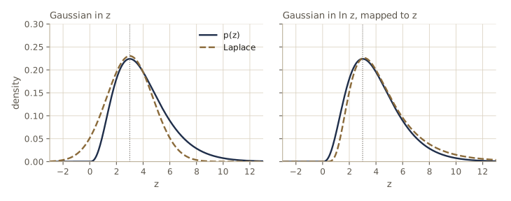
The Gaussian in \(z\) matches the peak but not the long right tail, and it places mass on negative \(z\). The approximation in \(\ln z\) roughly halves the total variation distance. Two further limitations are worth keeping in mind. A multimodal density has one Laplace approximation per mode, each blind to the others. And because the method uses only the value and curvature at one point, it can miss global properties of the density entirely; the variational methods of module 10 take a more global view. On the other hand, posteriors tend to become more Gaussian as the number of data points grows (a consequence of the central limit theorem), so the approximation is at its best exactly when we have a lot of data.
Model comparison and BIC
The Laplace approximation also estimates the normalizer. Integrating the unnormalized Gaussian,
\[Z = \int f(\mathbf{z})\,d\mathbf{z} \approx f(\mathbf{z}_0)\int\exp\left\{-\frac{1}{2}(\mathbf{z} - \mathbf{z}_0)^{\mathrm{T}}\mathbf{A}(\mathbf{z} - \mathbf{z}_0)\right\}d\mathbf{z} = f(\mathbf{z}_0)\frac{(2\pi)^{M/2}}{\lvert \mathbf{A} \rvert^{1/2}}.\]For our gamma example this is \(Z \approx 3^3e^{-3}\sqrt{2\pi \cdot 3} = 27e^{-3}\sqrt{6\pi}\). Since \(Z = \Gamma(4) = 3!\), this is Stirling’s approximation to a factorial — the Laplace approximation to the gamma integral.
Z_z = np.exp(log_f(z0)) * np.sqrt(2 * np.pi / A)
Z_u = np.exp(4 * u0 - np.exp(u0)) * np.sqrt(2 * np.pi / A_u)
print(f"exact Z = 6;  Laplace in z: {Z_z:.4f};  Laplace in ln z: {Z_u:.4f}")
exact Z = 6; Laplace in z: 5.8362; Laplace in ln z: 5.8765
The normalizer we care most about is the model evidence of module 03, \(p(\mathcal{D}) = \int p(\mathcal{D} \mid \boldsymbol{\theta})p(\boldsymbol{\theta})\,d\boldsymbol{\theta}\), the quantity Bayesian model comparison uses to rank models. Setting \(f(\boldsymbol{\theta}) = p(\mathcal{D} \mid \boldsymbol{\theta})p(\boldsymbol{\theta})\) and \(Z = p(\mathcal{D})\) in the formula above and taking logs,
\[\ln p(\mathcal{D}) \approx \ln p(\mathcal{D} \mid \boldsymbol{\theta}_{\text{MAP}}) + \underbrace{\ln p(\boldsymbol{\theta}_{\text{MAP}}) + \frac{M}{2}\ln(2\pi) - \frac{1}{2}\ln\lvert \mathbf{A} \rvert}_{\text{Occam factor}},\]where \(\boldsymbol{\theta}_{\text{MAP}}\) is the mode of the posterior and \(\mathbf{A} = -\nabla\nabla\ln\{p(\mathcal{D} \mid \boldsymbol{\theta})p(\boldsymbol{\theta})\}\) at the mode is the Hessian of the negative log posterior. The first term rewards fit. The Occam factor penalizes complexity: each well-determined parameter makes \(\lvert \mathbf{A} \rvert\) larger (a sharply peaked posterior occupies a small fraction of the prior’s volume), which lowers the evidence.
A rougher version follows if the prior is broad and the Hessian has full rank. Then \(\ln p(\boldsymbol{\theta}_{\text{MAP}})\) is roughly constant, and for \(N\) independent data points \(\mathbf{A} \approx N\overline{\mathbf{A}}\), a sum of \(N\) terms each of order one, so \(\ln\lvert \mathbf{A} \rvert \approx M\ln N + \text{const}\). Dropping terms that do not grow with \(N\) leaves the Bayesian information criterion (BIC),
\[\ln p(\mathcal{D}) \approx \ln p(\mathcal{D} \mid \boldsymbol{\theta}_{\text{MAP}}) - \frac{M}{2}\ln N,\]also called the Schwarz criterion. Compared with the Akaike criterion of module 01, which subtracts \(M\), it penalizes parameters more heavily once \(N > e^2 \approx 7\). BIC is easy to compute but crude. In particular, many parameters of a flexible model are poorly determined by the data, and then \(\ln\lvert \mathbf{A} \rvert\) grows much more slowly than \(M\ln N\), so BIC overcharges for them.
We compare logistic regression models with polynomial features of degree 0 to 6 on one-dimensional data whose true log odds is quadratic, \(a(x) = 1 + 1.5x - 0.8x^2\). The prior is \(\mathcal{N}(\mathbf{w} \mid \mathbf{0}, \alpha^{-1}\mathbf{I})\) with \(\alpha = 0.01\), broad compared with the weights. For this prior the Laplace evidence is
\[\ln p(\mathbf{t}) \approx \ln p(\mathbf{t} \mid \mathbf{w}_{\text{MAP}}) - \frac{\alpha}{2}\lVert \mathbf{w}_{\text{MAP}} \rVert^2 + \frac{M}{2}\ln\alpha - \frac{1}{2}\ln\lvert \mathbf{A} \rvert, \qquad \mathbf{A} = \alpha\mathbf{I} + \mathbf{\Phi}^{\mathrm{T}}\mathbf{R}\mathbf{\Phi}.\]def log_likelihood(w, Phi, t):
return -logistic_error(w, Phi, t)
def laplace_log_evidence(Phi, t, alpha):
"""Laplace estimate of ln p(t) for logistic regression, prior N(0, I / alpha)."""
M = Phi.shape[1]
w_map, _ = irls(Phi, t, alpha=alpha)
A = logistic_hessian(w_map, Phi, t, alpha)
log_ev = (log_likelihood(w_map, Phi, t) - 0.5 * alpha * w_map @ w_map
+ 0.5 * M * np.log(alpha) - 0.5 * np.linalg.slogdet(A)[1])
return log_ev, w_map, A
def poly_features(x, degree):
return np.vander(x / 3.0, degree + 1, increasing=True) # powers of u = x/3
rnge = np.random.default_rng(6)
N_e = 120
x_e = rnge.uniform(-3, 3, N_e)
t_e = (rnge.random(N_e) < expit(1.0 + 1.5 * x_e - 0.8 * x_e**2)).astype(float)
alpha_e = 0.01
print("degree M ln p(t|w_ML) Laplace ln p(t) BIC")
for d in range(7):
Phi_e = poly_features(x_e, d)
log_ev, _, _ = laplace_log_evidence(Phi_e, t_e, alpha_e)
w_ml, _ = irls(Phi_e, t_e, alpha=1e-8)
ll = log_likelihood(w_ml, Phi_e, t_e)
bic = ll - 0.5 * (d + 1) * np.log(N_e)
print(f"{d:6d} {d + 1:3d} {ll:14.2f} {log_ev:17.2f} {bic:8.2f}")
degree   M   ln p(t|w_ML)   Laplace ln p(t)     BIC
     0   1         -81.15            -85.14   -83.54
     1   2         -75.54            -82.87   -80.33
     2   3         -45.98            -54.76   -53.16
     3   4         -45.92            -55.78   -55.50
     4   5         -45.88            -56.39   -57.85
     5   6         -44.96            -56.60   -59.32
     6   7         -44.84            -56.95   -61.60
The maximized likelihood only increases with the degree, as it must for nested models. Both the Laplace evidence and BIC peak at degree 2, the true model; the evidence declines more gently afterwards, because the extra coefficients of the scaled powers are poorly determined and the Occam factor charges less for them than BIC’s blanket \(\frac{1}{2}\ln N\) per parameter.
How good is the Laplace estimate itself? For the two-parameter model we can compute the evidence almost exactly by importance sampling (module 11 has the details): draw \(\mathbf{w}^{(s)}\) from the Laplace Gaussian \(q\) and average \(p(\mathbf{t} \mid \mathbf{w}^{(s)})p(\mathbf{w}^{(s)})/q(\mathbf{w}^{(s)})\).
Phi_e1 = poly_features(x_e, 1)
log_ev1, w_map1, A1 = laplace_log_evidence(Phi_e1, t_e, alpha_e)
rng_is = np.random.default_rng(1)
L_A = np.linalg.cholesky(A1)                     # A = L L^T; w_map + L^-T eps ~ q
eps = rng_is.normal(size=(200000, 2))
W_s = w_map1 + np.linalg.solve(L_A.T, eps.T).T
a_s = W_s @ Phi_e1.T
log_lik = a_s @ t_e - np.logaddexp(0, a_s).sum(axis=1)
log_prior = stats.multivariate_normal(np.zeros(2), np.eye(2) / alpha_e).logpdf(W_s)
# ln q(w): since L^T (w - w_map) = eps, the quadratic form is just ||eps||^2
log_q = (-0.5 * np.sum(eps**2, axis=1) + np.sum(np.log(np.diag(L_A)))
         - np.log(2 * np.pi))
log_ev_is = logsumexp(log_lik + log_prior - log_q) - np.log(len(W_s))
print(f"degree 1: Laplace ln p(t) = {log_ev1:.3f}, "
      f"importance sampling = {log_ev_is:.3f}")
degree 1: Laplace ln p(t) = -82.873, importance sampling = -82.862
The two agree to within a few hundredths of a nat.
Bayesian logistic regression
Laplace approximation of the posterior
We now apply the Laplace approximation to the posterior of logistic regression. Because the result will be Gaussian, a Gaussian prior is the natural choice, \(p(\mathbf{w}) = \mathcal{N}(\mathbf{w} \mid \mathbf{m}_0, \mathbf{S}_0)\). The log posterior is
\[\ln p(\mathbf{w} \mid \mathbf{t}) = -\frac{1}{2}(\mathbf{w} - \mathbf{m}_0)^{\mathrm{T}}\mathbf{S}_0^{-1}(\mathbf{w} - \mathbf{m}_0) + \sum_{n=1}^{N}\left\{t_n\ln y_n + (1 - t_n)\ln(1 - y_n)\right\} + \text{const},\]with \(y_n = \sigma(\mathbf{w}^{\mathrm{T}}\boldsymbol{\phi}_n)\). Its maximum is the MAP solution \(\mathbf{w}_{\text{MAP}}\), which IRLS finds (with \(\mathbf{m}_0 = \mathbf{0}\) and \(\mathbf{S}_0 = \alpha^{-1}\mathbf{I}\) this is exactly our irls with the prior). The negative Hessian of the log posterior at the mode is the precision of the Gaussian approximation:
Compare this with Bayesian linear regression in module 03, where \(\mathbf{S}_N^{-1} = \mathbf{S}_0^{-1} + \beta\mathbf{\Phi}^{\mathrm{T}}\mathbf{\Phi}\): the constant noise precision \(\beta\) has become a per-point weight \(y_n(1 - y_n)\), large for points near the boundary and small for points the model is sure about.
Our data set is small on purpose, 15 points per class in the plane, with prior \(\alpha = 1\). As a check on the approximation, we estimate the true posterior mean by self-normalized importance sampling with \(q\) as the proposal.
rngl = np.random.default_rng(21)
n_l = 15
X_l = np.vstack([rngl.normal([-1.0, 0.5], 0.8, (n_l, 2)),
                 rngl.normal([1.0, -0.5], 0.8, (n_l, 2))])
t_l = np.r_[np.ones(n_l), np.zeros(n_l)]
Phi_l = add_bias(X_l)
alpha_l = 1.0

w_map, _ = irls(Phi_l, t_l, alpha=alpha_l)
# we need the covariance S_N itself; for 3 x 3 an explicit inverse is harmless
S_N = np.linalg.inv(logistic_hessian(w_map, Phi_l, t_l, alpha_l))
print("w_MAP =", w_map)
print("posterior standard deviations:", np.sqrt(np.diag(S_N)))

rng_q = np.random.default_rng(2)
W_q = rng_q.multivariate_normal(w_map, S_N, size=100000)
W_is = W_q[:20000]
# unnormalized log posterior
log_post = np.array([-logistic_error(v, Phi_l, t_l, alpha_l) for v in W_is])
log_q = stats.multivariate_normal(w_map, S_N).logpdf(W_is)
wts = np.exp(log_post - log_q - logsumexp(log_post - log_q))
print("posterior mean by importance sampling:", wts @ W_is)
print(f"effective sample size: {1 / np.sum(wts**2):.0f} of 20000")
w_MAP = [-0.3069 -1.6215  1.3761]
posterior standard deviations: [0.538  0.5625 0.6081]
posterior mean by importance sampling: [-0.298  -1.8137  1.4814]
effective sample size: 14178 of 20000
The true posterior mean lies noticeably further from the origin than the mode, in the direction of stronger weights: with only 30 points the posterior is skewed, and a Gaussian centered at the mode cannot represent that. The high effective sample size says that \(q\) nevertheless covers the posterior well.
Predictive distribution
To classify a new point with feature vector \(\boldsymbol{\phi}\), we average the model’s prediction over the posterior:
\[p(\mathcal{C}_1 \mid \boldsymbol{\phi}, \mathbf{t}) = \int\sigma(\mathbf{w}^{\mathrm{T}}\boldsymbol{\phi})\,p(\mathbf{w} \mid \mathbf{t})\,d\mathbf{w} \approx \int\sigma(\mathbf{w}^{\mathrm{T}}\boldsymbol{\phi})\,q(\mathbf{w})\,d\mathbf{w}.\]The integrand depends on \(\mathbf{w}\) only through the scalar \(a = \mathbf{w}^{\mathrm{T}}\boldsymbol{\phi}\). Under \(q\), \(a\) is a linear function of a Gaussian vector, so it is Gaussian (module 02), with
\[\mu_a = \mathbb{E}[a] = \mathbf{w}_{\text{MAP}}^{\mathrm{T}}\boldsymbol{\phi}, \qquad \sigma_a^2 = \operatorname{var}[a] = \boldsymbol{\phi}^{\mathrm{T}}\mathbf{S}_N\boldsymbol{\phi}.\]The \(M\)-dimensional integral collapses to a one-dimensional one,
\[p(\mathcal{C}_1 \mid \boldsymbol{\phi}, \mathbf{t}) \approx \int\sigma(a)\,\mathcal{N}(a \mid \mu_a, \sigma_a^2)\,da .\](Note that \(\sigma_a^2\) has the same form as the predictive variance of Bayesian linear regression in module 03, without the noise term.) This integral of a sigmoid against a Gaussian has no closed form, but a probit against a Gaussian does. So we approximate the sigmoid by a rescaled probit, \(\sigma(a) \approx \Phi(\lambda a)\), and choose \(\lambda\) so that the two have the same slope at \(a = 0\): \(\sigma'(0) = \frac{1}{4}\) and \(\frac{d}{da}\Phi(\lambda a)\rvert_0 = \lambda/\sqrt{2\pi}\), so \(\lambda = \sqrt{2\pi}/4\), that is, \(\lambda^2 = \pi/8\). The probit–Gaussian integral we need is, for \(a \sim \mathcal{N}(\mu, \sigma^2)\),
\[\int\Phi(\lambda a)\,\mathcal{N}(a \mid \mu, \sigma^2)\,da = \Phi\left(\frac{\mu}{(\lambda^{-2} + \sigma^2)^{1/2}}\right).\]The proof uses the definition of \(\Phi\) as a probability. Let \(\varepsilon \sim \mathcal{N}(0, 1)\) be independent of \(a\). Then \(\Phi(\lambda a) = \Pr(\varepsilon \le \lambda a \mid a)\), and averaging over \(a\) gives \(\Pr(\varepsilon/\lambda - a \le 0)\). The variable \(\varepsilon/\lambda - a\) is Gaussian with mean \(-\mu\) and variance \(\lambda^{-2} + \sigma^2\), so the probability is \(\Phi\left(\mu/\sqrt{\lambda^{-2} + \sigma^2}\right)\).
Now use the approximation in reverse on the right side:
\[\Phi\left(\frac{\mu}{\sqrt{\lambda^{-2} + \sigma^2}}\right) = \Phi\left(\frac{\lambda\mu}{\sqrt{1 + \lambda^2\sigma^2}}\right) \approx \sigma\left(\frac{\mu}{\sqrt{1 + \pi\sigma^2/8}}\right).\]So
\[\int\sigma(a)\,\mathcal{N}(a \mid \mu, \sigma^2)\,da \approx \sigma\left(\kappa(\sigma^2)\,\mu\right), \qquad \kappa(\sigma^2) = \left(1 + \frac{\pi\sigma^2}{8}\right)^{-1/2},\]and the approximate predictive distribution is
Result. \(p(\mathcal{C}_1 \mid \boldsymbol{\phi}, \mathbf{t}) \approx \sigma\left(\kappa(\sigma_a^2)\,\mu_a\right)\), with \(\mu_a = \mathbf{w}_{\text{MAP}}^{\mathrm{T}}\boldsymbol{\phi}\) and \(\sigma_a^2 = \boldsymbol{\phi}^{\mathrm{T}}\mathbf{S}_N\boldsymbol{\phi}\).
We check each approximation in turn: the probit fit to the sigmoid, the probit–Gaussian identity (against numerical integration), and the final formula (against numerical integration over \(a\) and against Monte Carlo over \(\mathbf{w}\)).
lam = np.sqrt(np.pi / 8)
a_grid = np.linspace(-10, 10, 20001)
gap = np.abs(expit(a_grid) - ndtr(lam * a_grid)).max()
print(f"max |sigma(a) - Phi(lambda a)| = {gap:.4f}")

gh_x, gh_w = np.polynomial.hermite_e.hermegauss(80)  # Gauss-Hermite nodes for N(0, 1)
def gauss_average(func, mu, s2):
    """E[func(a)] for a ~ N(mu, s2), by 80-point Gauss-Hermite quadrature."""
    return np.sum(gh_w * func(mu + np.sqrt(s2) * gh_x)) / np.sqrt(2 * np.pi)

mu_c, s2_c = 1.3, 4.0
lhs = gauss_average(lambda v: ndtr(lam * v), mu_c, s2_c)
print(f"probit identity: quadrature {lhs:.6f}, "
      f"formula {ndtr(mu_c / np.sqrt(1 / lam**2 + s2_c)):.6f}")

def predictive_probit(Phi_new, w_map, S_N):
    mu_a = Phi_new @ w_map
    s2_a = np.einsum("ij,jk,ik->i", Phi_new, S_N, Phi_new)  # phi^T S_N phi, per row
    return expit(mu_a / np.sqrt(1 + np.pi * s2_a / 8)), mu_a, s2_a

n_hat = w_map[1:] / np.linalg.norm(w_map[1:])      # unit normal to the MAP boundary
along = np.array([n_hat[1], -n_hat[0]])  # unit direction along the boundary
points = np.array([0.5 * n_hat + k * along for k in [0, 3, 6, 10]]
                  + [2 * n_hat, 2 * n_hat + 8 * along])
p_approx, mu_a, s2_a = predictive_probit(add_bias(points), w_map, S_N)
mc = expit(W_q @ add_bias(points).T).mean(axis=0)         # Monte Carlo over w ~ q
print("    point x        mu_a  sigma_a^2     MAP   quadrature  probit  Monte Carlo")
for i, pt in enumerate(points):
    quad = gauss_average(expit, mu_a[i], s2_a[i])
    print(f"({pt[0]:5.2f},{pt[1]:5.2f})  {mu_a[i]:6.3f} {s2_a[i]:9.3f} "
          f"{expit(mu_a[i]):7.4f} {quad:10.4f} {p_approx[i]:9.4f} {mc[i]:9.4f}")
max |sigma(a) - Phi(lambda a)| = 0.0177
probit identity: quadrature 0.694304, formula 0.694304
    point x        mu_a  sigma_a^2     MAP   quadrature  probit  Monte Carlo
(-0.38, 0.32)   0.756     0.323  0.6806     0.6693    0.6710    0.6693
( 1.56, 2.61)   0.756     3.114  0.6806     0.6210    0.6242    0.6216
( 3.50, 4.90)   0.756    12.000  0.6806     0.5771    0.5785    0.5779
( 6.09, 7.95)   0.756    33.331  0.6806     0.5498    0.5502    0.5504
(-1.52, 1.29)   3.947     1.465  0.9810     0.9646    0.9587    0.9647
( 3.65, 7.39)   3.947    23.121  0.9810     0.7791    0.7761    0.7801
The rescaled probit stays within about 0.02 of the sigmoid everywhere, the identity holds to the digits shown, and the final approximation agrees with the exact one-dimensional integral and with Monte Carlo to within about 0.006.
The table also shows the main qualitative effect. The first four points all have the same \(\mu_a\), so the MAP model gives all of them the same probability. But they lie at increasing distances from the data along the boundary, \(\sigma_a^2\) grows, \(\kappa\) shrinks, and the predictive probability slides toward one half. The last two rows show the same thing for points the MAP model is sure about: far from the data, a confidence of 0.98 becomes one of about 0.78. The model is saying that it has seen no data out there, so the orientation of its boundary is uncertain.
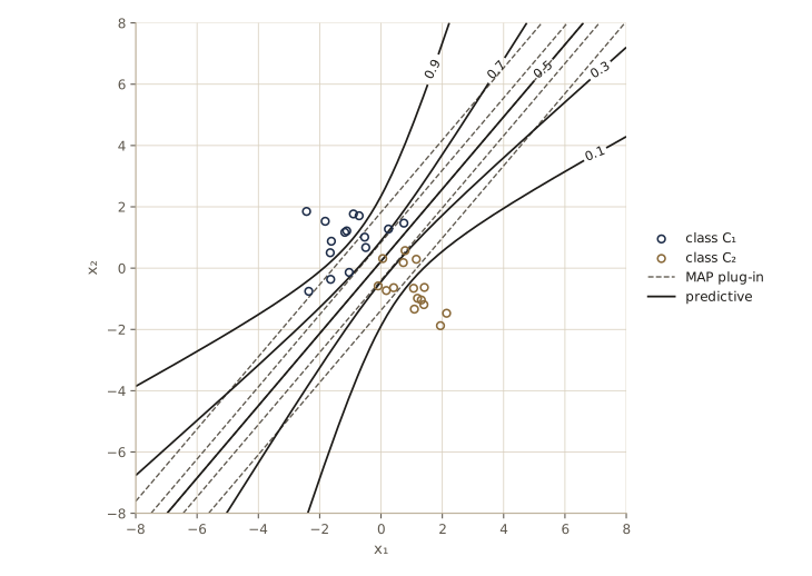
Note. The predictive probability is one half exactly when \(\mu_a = 0\), which is the MAP decision boundary. So if we only need the most probable class with equal misclassification costs, averaging over the posterior changes nothing. It matters when the probabilities themselves matter: with asymmetric losses, a reject option, or when predictions are combined with other models, all from the decision theory of module 01.
Summary
| Model | What it assumes | How it is fit | Output |
|---|---|---|---|
| Least squares, 1-of-\(K\) targets | nothing probabilistic (implicitly Gaussian noise) | closed form, \(\widetilde{\mathbf{W}} = \widetilde{\mathbf{X}}^{\dagger}\mathbf{T}\) | scores; fails with outliers and sandwiched classes |
| Fisher’s discriminant | classes separated by projection | closed form, \(\mathbf{w} \propto \mathbf{S}_W^{-1}(\mathbf{m}_2 - \mathbf{m}_1)\) | a direction; threshold chosen separately |
| Perceptron | linearly separable data | perceptron rule, at most \((R/\gamma)^2\) updates | label only; no convergence otherwise |
| Gaussian generative (shared \(\boldsymbol{\Sigma}\)) | \(p(\mathbf{x} \mid \mathcal{C}_k) = \mathcal{N}(\boldsymbol{\mu}_k, \boldsymbol{\Sigma})\) | ML in closed form: class fractions, means, pooled covariance | posterior, linear boundary |
| Gaussian generative (own \(\boldsymbol{\Sigma}_k\)) | \(p(\mathbf{x} \mid \mathcal{C}_k) = \mathcal{N}(\boldsymbol{\mu}_k, \boldsymbol{\Sigma}_k)\) | ML in closed form | posterior, quadratic boundary |
| Naive Bayes | features independent given the class | counts (plus pseudo-counts) | posterior, linear in binary features |
| Logistic / softmax regression | \(p(\mathcal{C}_k \mid \boldsymbol{\phi})\) is a sigmoid / softmax of \(\mathbf{w}_k^{\mathrm{T}}\boldsymbol{\phi}\) | IRLS (Newton), convex; needs a prior on separable data | posterior |
| Probit regression | noisy Gaussian threshold | Newton, convex | posterior, lighter tails |
| Bayesian logistic regression | Gaussian prior on \(\mathbf{w}\) | Laplace approximation at \(\mathbf{w}_{\text{MAP}}\) | predictive \(\sigma(\kappa(\sigma_a^2)\mu_a)\) |
Ideas to carry forward:
- Squared error is the wrong loss for labels. The cross-entropy of a Bernoulli or categorical likelihood is the right one, and with the canonical link its gradient is always “error times feature”, \(\sum_n(y_n - t_n)\boldsymbol{\phi}_n\). Backpropagation in module 05 starts from exactly this quantity at the output layer.
- Generative and discriminative models can produce the same functional form, \(\sigma(\mathbf{w}^{\mathrm{T}}\boldsymbol{\phi})\). The generative model fits more parameters under stronger assumptions and wins with little data when the assumptions hold; the discriminative model fits the posterior directly and is more robust to misspecification.
- Newton’s method turns a convex, nearly quadratic problem into a few weighted least-squares solves; IRLS reappears in the relevance vector machine (module 07) and Gaussian-process classification (module 06).
- The Laplace approximation — find the mode, take the Hessian, use a Gaussian — gives approximate posteriors, predictive distributions, and evidence. It is local and blind to skew and to other modes, which is the motivation for the methods of modules 10 and 11.
Exercises
- Show that if the convex hulls of two point sets intersect, no hyperplane can separate them, and conversely that two linearly separable sets have disjoint convex hulls. Then construct four points in the plane that are not linearly separable and verify with
perceptronthat it does not converge. - For the \(K\)-class discriminant, suppose all \(K\) weight vectors \(\mathbf{w}_k\) are replaced by \(\mathbf{w}_k + \mathbf{v}\) and all biases by \(w_{k0} + c\) for a common vector \(\mathbf{v}\) and scalar \(c\). Show that the classifier is unchanged. How does this relate to the zero eigenvalues of the softmax Hessian?
- Prove the two-class scatter decomposition \(\mathbf{S}_T = \mathbf{S}_W + \frac{N_1N_2}{N}\mathbf{S}_B\) used in the relation to least squares, and its \(K\)-class version \(\mathbf{S}_T = \mathbf{S}_W + \mathbf{S}_B\) with \(\mathbf{S}_B\) as defined for multiple classes. Then show that the scalar \(c\) in the least-squares derivation of Fisher’s direction is positive.
- The perceptron bound \((R/\gamma)^2\) depends on the scale of the features only through the ratio. Show that centering the inputs (subtracting their mean before adding the constant feature) can change \(R/\gamma\), and measure the effect on the number of updates for the perceptron data of this module.
- For the two-class Gaussian model with shared covariance, show that the log odds \(a(\mathbf{x})\) is unchanged if the same invertible linear map is applied to all inputs and the model is refitted. Is the same true for logistic regression? For naive Bayes with Gaussian features (independent features within each class)?
- Derive the Hessian of the probit error function given in the notes, including the fact that \(\lambda(z + \lambda) > 0\) for every \(z\), where \(\lambda = \mathcal{N}(z \mid 0, 1)/\Phi(z)\). (Hint: show that \(\lambda(z)\) is the mean of a standard Gaussian variable conditioned to exceed \(-z\); a conditional mean must lie above the lower limit.)
- Show that the multiclass cross-entropy Hessian is positive semidefinite: for any \(\mathbf{u} = (\mathbf{u}_1, \dots, \mathbf{u}_K)\), write \(\mathbf{u}^{\mathrm{T}}\mathbf{H}\mathbf{u}\) as a sum over data points of the variance of \(\mathbf{u}_k^{\mathrm{T}}\boldsymbol{\phi}_n\) under the distribution \(k \sim y_{nk}\).
- Modify
irlsto accept a general Gaussian prior \(\mathcal{N}(\mathbf{m}_0, \mathbf{S}_0)\). Use it to fit the ring data with a prior that pulls the weights toward a hand-chosen value, and describe how the boundary changes as the prior gets tighter. - Implement gradient descent for softmax regression and compare the number of iterations it needs with
fit_softmax_newtonon the three-class data. Then fit the three-class data with a one-versus-the-rest set of logistic regressions and report the fraction of the grid claimed by zero or by two or more classifiers. - Derive the BIC from the Laplace evidence for a Gaussian prior \(\mathcal{N}(\boldsymbol{\theta} \mid \mathbf{m}, \mathbf{V}_0)\), stating exactly which terms you drop and why they do not grow with \(N\). Then repeat the polynomial experiment with \(N = 30\) and \(N = 1000\) data points and report which degrees the evidence and BIC choose.
- For the gamma example, compute the Laplace approximation to \(\ln\Gamma(n + 1) = \ln n!\) for \(n = 1, 2, 5, 10, 50\) using \(f(z) = z^ne^{-z}\), compare with
scipy.special.gammaln, and show that the relative error of \(Z\) is close to \(1/(12n)\). - In your own words: why does Bayesian logistic regression give probabilities closer to one half far from the training data, while the MAP model does not? Would the same happen if we added thousands more data points spread over the whole plane?
Going further
- C. M. Bishop, Pattern Recognition and Machine Learning, chapter 4 — the source for this module. Exercises 4.1 (convex hulls), 4.4–4.6 (Fisher and least squares), 4.9–4.11 (generative maximum likelihood and naive Bayes), 4.13–4.15 and 4.17–4.20 (gradients and Hessians of the logistic and softmax models), and 4.22–4.26 (Laplace evidence, BIC, and the probit approximation) pair well with the sections above. Section 10.6 revisits Bayesian logistic regression with a variational approximation.
- R. A. Fisher, “The use of multiple measurements in taxonomic problems”, Annals of Eugenics, 1936 — the original linear discriminant, introduced with the iris data.
- F. Rosenblatt, “The perceptron: a probabilistic model for information storage and organization in the brain”, Psychological Review, 1958.
- J. A. Nelder and R. W. M. Wedderburn, “Generalized linear models”, Journal of the Royal Statistical Society, Series A, 1972 — the unifying framework behind the canonical link result and IRLS.
- G. Schwarz, “Estimating the dimension of a model”, The Annals of Statistics, 1978 — the Bayesian information criterion.
- D. J. C. MacKay, “The evidence framework applied to classification networks”, Neural Computation, 1992 — the Laplace approximation and the moderated (predictive) output for classifiers.
These notes follow the chapters of C. M. Bishop, Pattern Recognition and Machine Learning (Springer, 2006), the course text, which Microsoft Research makes freely available as a PDF. The explanations, code, figures, and exercises here are written for this course; the book remains the reference, with the full derivations and many more exercises.