CSE 474/574 · Module 01 · Week 1
Introduction: Curve Fitting, Probability, and Decisions
Polynomial curve fitting and overfitting, probability and Bayes' theorem, model selection, the curse of dimensionality, decision theory, and information theory.
Companion reading: Bishop, Pattern Recognition and Machine Learning, chapter 1, “Introduction”
By the end of this module you can
- Fit polynomials by least squares and by regularized least squares in NumPy, and use training and test error to recognize overfitting.
- Apply the sum and product rules and Bayes’ theorem, and transform a probability density under a change of variables.
- Derive the maximum likelihood estimates of a Gaussian’s mean and variance, and show by algebra and by simulation that the variance estimate is biased.
- Explain least squares as maximum likelihood under Gaussian noise and ridge regression as a MAP estimate under a Gaussian prior, and compute a Bayesian predictive distribution for curve fitting.
- Choose a model’s complexity with a validation set or S-fold cross-validation, and state what information criteria try to do.
- Show with numbers why high-dimensional spaces defeat grid-based methods and low-dimensional intuition.
- Derive the decision rules that minimize the misclassification rate and the expected loss, add a reject option, and say which summary of the conditional distribution each regression loss asks for.
- Compute entropy, differential entropy, conditional entropy, KL divergence, and mutual information, and prove that the KL divergence is never negative.
Contents
- Learning from examples
- Polynomial curve fitting
- Probability theory
- Model selection
- The curse of dimensionality
- Decision theory
- Information theory
- Summary
- Exercises
- Going further
This course is about building programs whose behavior comes from data rather than from hand-written rules. You show the program many examples, it adjusts a model to fit them, and then it makes predictions or decisions about cases it has never seen. The whole difficulty sits in that last phrase. Fitting the examples you have is easy; doing well on new ones requires assumptions, and this module introduces the three tools we use to state and reason about those assumptions for the rest of the semester: probability theory, decision theory, and information theory.
We start from one small problem, fitting a curve to ten noisy points, and keep coming back to it. It is simple enough that every number can be checked by hand, yet it already shows overfitting, regularization, maximum likelihood, Bayesian inference, and model selection. After that we look at why many input dimensions make everything harder, how to turn probabilities into decisions, and how to measure information.
How the notes work. There is one module per chapter of Bishop’s Pattern Recognition and Machine Learning, the course text: module 01 follows chapter 1, module 02 follows chapter 2, and so on. The notes are written for this course and do not copy the book; each module says which book sections hold the full derivations. Every idea comes with NumPy code. The code cells in a module run top to bottom in one Python session, and the output shown under each cell is the real output of that run, so you can reproduce every number. Each module ends with a summary, exercises that mix derivations with coding, and pointers for further reading.
What the course expects. You should be comfortable with linear algebra (matrix products, inverses, eigenvalues, solving linear systems), probability at the level of a first course (random variables, expectation, variance, the Gaussian), multivariable calculus (gradients, setting derivatives to zero, the chain rule), and Python with NumPy (arrays, broadcasting, vectorized arithmetic). We review what we need as we go, but we do not teach these from scratch.
In practice. To follow along, open a notebook, paste the cells in order, and run them. Every random number comes from a seeded generator, so your output should match ours digit for digit on the same NumPy version. If a result looks surprising, change a seed or a size and rerun: most of the claims in these notes are cheap to test.
Learning from examples
Here is the vocabulary we will use all semester. Suppose we want to read handwritten digits. Each image is a grid of pixel intensities, which we flatten into an input vector \(\mathbf{x}\). Writing rules by hand (“a 7 has a horizontal stroke at the top…”) breaks down quickly, because handwriting varies too much. Instead we collect a training set of \(N\) examples \(\mathbf{x}_1, \dots, \mathbf{x}_N\), each paired with a target \(\mathbf{t}_n\) that records the correct answer, and use them to adjust the parameters of a model. The result is a function \(\mathbf{y}(\mathbf{x})\) that maps a new input to a prediction.
Adjusting the parameters is called training or learning. We judge the result on a test set: examples that were not used in training. The ability to perform well on new inputs is called generalization, and it is the central goal. The training set can never cover more than a tiny fraction of all possible inputs, so a model that merely memorizes it is useless.
Inputs are often transformed before learning, for example by centering and rescaling each digit image. This step is called preprocessing or feature extraction. It can make the learning problem easier or faster, but it can also discard information the model needed. Whatever preprocessing we choose, test inputs must go through exactly the same steps.
Problems come in a few broad kinds:
- In supervised learning the training data include targets. When the target is one of a finite set of categories, the task is classification; when it is one or more continuous numbers, it is regression.
- In unsupervised learning there are no targets. We may look for groups of similar inputs (clustering), estimate the distribution that generated the inputs (density estimation), or map the data to two or three dimensions to look at it (visualization).
- In reinforcement learning an agent takes actions and receives rewards, and it must discover good actions by trial and error. It faces problems we will not treat in this course, such as balancing exploration of new actions against exploitation of known good ones, and deciding which of many earlier actions deserves credit for a late reward.
Most of this course is supervised learning, with unsupervised learning in modules 09 and 12.
Polynomial curve fitting
The data
We generate data ourselves so that we know the truth. The inputs \(x\) are ten evenly spaced points in \([0, 1]\), and each target is \(t = \sin(2\pi x) + \epsilon\), where the noise \(\epsilon\) is Gaussian with mean zero and standard deviation 0.3. The learner sees only the pairs \((x_n, t_n)\); the sine curve is hidden from it. We also draw a large test set from the same source, with random inputs, to measure how well a fitted curve generalizes.
import numpy as np
from scipy.special import gammaln, erf

np.set_printoptions(precision=4, suppress=True)
rng = np.random.default_rng(474)

def make_data(N, rng, sigma=0.3, random_x=False):
    """N noisy observations t = sin(2 pi x) + noise; x evenly spaced or uniform in [0, 1]."""
    x = rng.uniform(0, 1, N) if random_x else np.linspace(0, 1, N)
    t = np.sin(2 * np.pi * x) + rng.normal(0, sigma, N)
    return x, t

x, t = make_data(10, rng)                               # the training set
x_test, t_test = make_data(1000, rng, random_x=True)    # a large test set
print("x =", x)
print("t =", t)
x = [0.     0.1111 0.2222 0.3333 0.4444 0.5556 0.6667 0.7778 0.8889 1.    ]
t = [ 0.2222  0.5873  1.3955  0.8663 -0.1451 -0.2042 -0.8661 -0.7862 -0.7253
  0.1245]
Least squares
We fit a polynomial of order \(M\),
\[y(x, \mathbf{w}) = w_0 + w_1 x + w_2 x^2 + \dots + w_M x^M = \sum_{j=0}^{M} w_j x^j .\]It is a nonlinear function of \(x\) but a linear function of the coefficients \(\mathbf{w} = (w_0, \dots, w_M)^{\mathrm{T}}\), and that is what makes it easy to fit. Models that are linear in their parameters are the subject of module 03.
To fit, we pick the \(\mathbf{w}\) that makes the curve pass close to the targets. The usual measure of misfit is the sum-of-squares error function
\[E(\mathbf{w}) = \frac{1}{2} \sum_{n=1}^{N} \bigl( y(x_n, \mathbf{w}) - t_n \bigr)^2 ,\]which is zero only if the curve goes through every point. (The factor \(\tfrac12\) just tidies the derivative.) To minimize it, collect the powers of the inputs in the \(N \times (M+1)\) design matrix \(\mathbf{\Phi}\) with entries \(\Phi_{nj} = x_n^j\). Then the vector of predictions is \(\mathbf{\Phi}\mathbf{w}\), and
\[E(\mathbf{w}) = \tfrac{1}{2} \lVert \mathbf{\Phi}\mathbf{w} - \mathbf{t} \rVert^2 = \tfrac12 (\mathbf{\Phi}\mathbf{w} - \mathbf{t})^{\mathrm{T}}(\mathbf{\Phi}\mathbf{w} - \mathbf{t}).\]This is a quadratic function of \(\mathbf{w}\), so it has a single minimum where the gradient vanishes:
\[\nabla E(\mathbf{w}) = \mathbf{\Phi}^{\mathrm{T}} (\mathbf{\Phi}\mathbf{w} - \mathbf{t}) = \mathbf{0} \quad\Longrightarrow\quad \mathbf{\Phi}^{\mathrm{T}}\mathbf{\Phi}\, \mathbf{w}^\star = \mathbf{\Phi}^{\mathrm{T}} \mathbf{t}.\]These \(M+1\) linear equations are the normal equations. (The minimum is unique when \(\mathbf{\Phi}\) has linearly independent columns, which holds here as long as \(N \ge M + 1\) and the \(x_n\) are distinct.) To compare errors across data sets of different sizes and in the units of \(t\), we report the root-mean-square error \(E_{\mathrm{RMS}} = \sqrt{2E(\mathbf{w}^\star)/N}\).
def design_matrix(x, M):
    """Phi[n, j] = x_n ** j for j = 0..M; shape (N, M + 1)."""
    return x[:, None] ** np.arange(M + 1)

def fit_poly(x, t, M, lam=0.0):
    """Coefficients of an order-M polynomial minimizing E(w) + (lam / 2) ||w||^2."""
    Phi = design_matrix(x, M)
    if lam == 0.0:
        return np.linalg.lstsq(Phi, t, rcond=None)[0]      # least squares, via an SVD
    A = Phi.T @ Phi + lam * np.eye(M + 1)                  # regularized normal equations
    return np.linalg.solve(A, Phi.T @ t)

def predict(w, x):
    return design_matrix(x, len(w) - 1) @ w

def rms_error(w, x, t):
    """E_RMS = sqrt(2 E(w) / N) = square root of the mean squared residual."""
    return np.sqrt(np.mean((predict(w, x) - t) ** 2))

# check (M = 3): lstsq agrees with the normal equations, and the gradient vanishes
Phi3 = design_matrix(x, 3)
w3 = fit_poly(x, t, 3)
w3_normal = np.linalg.solve(Phi3.T @ Phi3, Phi3.T @ t)
print("w* (M=3):", w3)
print(f"max difference from normal equations: {np.abs(w3 - w3_normal).max():.2e}")
print(f"norm of gradient at w*: {np.linalg.norm(Phi3.T @ (Phi3 @ w3 - t)):.2e}")
w* (M=3): [  0.1701   9.464  -30.0149  20.54  ]
max difference from normal equations: 1.63e-11
norm of gradient at w*: 3.91e-14
The two ways of solving agree, and the gradient at the solution is zero up to rounding. So the fit works; the interesting question is which \(M\) to use.
The order of the polynomial and overfitting
Let us fit orders \(M = 0, 1, 3, 9\) and measure the error on the training set and on the test set.
for M in [0, 1, 3, 9]:
    w = fit_poly(x, t, M)
    print(f"M = {M}:  train E_RMS = {rms_error(w, x, t):.3f}   "
          f"test E_RMS = {rms_error(w, x_test, t_test):.3f}")
M = 0:  train E_RMS = 0.710   test E_RMS = 0.789
M = 1:  train E_RMS = 0.544   test E_RMS = 0.567
M = 3:  train E_RMS = 0.213   test E_RMS = 0.320
M = 9:  train E_RMS = 0.000   test E_RMS = 0.763
A constant (\(M = 0\)) and a line (\(M = 1\)) cannot bend enough to follow a sine wave, and both errors are large. The cubic does well on both sets. With \(M = 9\) the polynomial has ten coefficients for ten points, so it passes through every training point and its training error is zero, but its test error is more than twice the cubic’s. The figure shows why: to hit every noisy point the curve oscillates wildly between them.
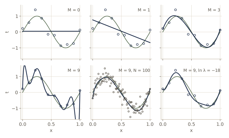
This gap between a small training error and a large test error is overfitting: the model has fit the noise in this particular training set rather than the regularity underneath. Here is the whole range of orders:
print(" M   train   test")
for M in range(10):
    w = fit_poly(x, t, M)
    print(f"{M:2d}   {rms_error(w, x, t):.3f}   {rms_error(w, x_test, t_test):.3f}")
 M   train   test
 0   0.710   0.789
 1   0.544   0.567
 2   0.539   0.567
 3   0.213   0.320
 4   0.209   0.326
 5   0.204   0.318
 6   0.148   0.342
 7   0.114   0.364
 8   0.102   0.392
 9   0.000   0.763
The training error can only go down as \(M\) grows, because each larger family of polynomials contains the smaller ones. The test error falls, flattens out between \(M = 3\) and \(M = 5\), and then climbs. The order-9 fit is puzzling at first: the sine function has a power series containing all odd powers of \(x\), so a larger polynomial should be able to approximate it at least as well. The coefficients tell us what went wrong.
ws = {M: fit_poly(x, t, M) for M in [0, 1, 3, 9]}
print("       " + "".join(f"{'M = ' + str(M):>13}" for M in ws))
for j in range(10):
    row = "".join(f"{ws[M][j]:13.2f}" if j <= M else " " * 13 for M in ws)
    print(f"w_{j}  " + row)
               M = 0        M = 1        M = 3        M = 9
w_0           0.05         0.76         0.17         0.22
w_1                       -1.43         9.46       109.17
w_2                                   -30.01     -2665.18
w_3                                    20.54     26129.80
w_4                                            -130988.76
w_5                                             373490.32
w_6                                            -631601.66
w_7                                             627147.43
w_8                                            -337682.21
w_9                                              76061.00
As \(M\) increases, the coefficients grow enormous, with alternating signs that nearly cancel at the data points. The flexible model has used its freedom to chase the noise on each point. Two things help: more data and regularization.
More data
With the order fixed at 9, draw larger training sets from the same source.
for N in [15, 100]:
    xN, tN = make_data(N, rng)
    wN = fit_poly(xN, tN, 9)
    print(f"N = {N:3d}:  train E_RMS = {rms_error(wN, xN, tN):.3f}   "
          f"test E_RMS = {rms_error(wN, x_test, t_test):.3f}   max |w_j| = {np.abs(wN).max():.0f}")
x100, t100 = xN, tN     # keep the N = 100 set for later
N =  15:  train E_RMS = 0.216   test E_RMS = 0.373   max |w_j| = 46119
N = 100:  train E_RMS = 0.277   test E_RMS = 0.316   max |w_j| = 31575
With 100 points, the order-9 polynomial no longer has enough freedom to thread through every point, and its test error comes close to the noise level of 0.3, which is the best any predictor can do. A common rule of thumb says the number of data points should be several times the number of parameters. The rule is not wrong, but it is unsatisfying: it ties model size to the amount of data, when the complexity we need should depend on the problem. Later in this module we will see that least squares is a special case of maximum likelihood, which is where the tendency to overfit comes from, and that a Bayesian treatment of the same model avoids it.
Watch out. Solving the normal equations directly can lose most of your digits. The matrix \(\mathbf{\Phi}^{\mathrm{T}}\mathbf{\Phi}\) has a condition number that is the square of \(\mathbf{\Phi}\)’s, and for polynomial features on \([0, 1]\) that number explodes with the order. Prefer
np.linalg.lstsq(or a QR or Cholesky factorization with regularization), and never form an explicit inverse withnp.linalg.invto solve a system.
for M in [3, 6, 9]:
    Phi = design_matrix(x, M)
    print(f"M = {M}:  cond(Phi) = {np.linalg.cond(Phi):.1e}   "
          f"cond(Phi^T Phi) = {np.linalg.cond(Phi.T @ Phi):.1e}")
M = 3:  cond(Phi) = 9.9e+01   cond(Phi^T Phi) = 9.8e+03
M = 6:  cond(Phi) = 2.0e+04   cond(Phi^T Phi) = 4.1e+08
M = 9:  cond(Phi) = 1.5e+07   cond(Phi^T Phi) = 2.3e+14
Double precision carries about 16 significant digits, and solving a system loses roughly as many digits as the base-10 logarithm of its condition number. For \(M = 9\) that leaves only one or two reliable digits if we go through \(\mathbf{\Phi}^{\mathrm{T}}\mathbf{\Phi}\), and about nine if we work with \(\mathbf{\Phi}\) directly, as lstsq does.
Regularization
The second remedy keeps the ten points and the ten coefficients but penalizes large coefficients. We minimize the regularized error
\[\widetilde{E}(\mathbf{w}) = \frac{1}{2} \sum_{n=1}^{N} \bigl( y(x_n, \mathbf{w}) - t_n \bigr)^2 + \frac{\lambda}{2} \lVert \mathbf{w} \rVert^2 ,\]where \(\lambda \ge 0\) sets the strength of the penalty relative to the data term. Setting the gradient to zero exactly as before gives
\[\bigl( \mathbf{\Phi}^{\mathrm{T}}\mathbf{\Phi} + \lambda \mathbf{I} \bigr) \mathbf{w}^\star = \mathbf{\Phi}^{\mathrm{T}} \mathbf{t}.\]Adding \(\lambda \mathbf{I}\) also makes the system well conditioned, which is why fit_poly can use np.linalg.solve when \(\lambda > 0\). In statistics this is ridge regression; in neural networks it is called weight decay; generally, penalties of this kind are called shrinkage methods because they pull coefficients toward zero. (Often \(w_0\) is left out of the penalty, so that shifting all targets by a constant does not change the fit; we keep it in for simplicity.)
lams = {"0 (none)": 0.0, "-18": np.exp(-18), "0": 1.0}
wl = {}
for name, lam in lams.items():
    wl[name] = fit_poly(x, t, 9, lam)
    print(f"ln lambda = {name:>8}:  train E_RMS = {rms_error(wl[name], x, t):.3f}   "
          f"test E_RMS = {rms_error(wl[name], x_test, t_test):.3f}   "
          f"max |w_j| = {np.abs(wl[name]).max():.2f}")
ln lambda = 0 (none):  train E_RMS = 0.000   test E_RMS = 0.763   max |w_j| = 631601.66
ln lambda =      -18:  train E_RMS = 0.139   test E_RMS = 0.335   max |w_j| = 1047.72
ln lambda =        0:  train E_RMS = 0.540   test E_RMS = 0.600   max |w_j| = 0.43
A tiny penalty, \(\ln \lambda = -18\) (that is, \(\lambda \approx 1.5 \times 10^{-8}\)), shrinks the largest coefficient by a factor of about 600 and more than halves the test error. A large penalty, \(\lambda = 1\), flattens the curve too much: training and test error are both high again. So \(\lambda\) now plays the role that \(M\) played, controlling the effective complexity of the model. Sweeping it:
ln_lams = np.arange(-35, 1, 1.0)
train_l = [rms_error(fit_poly(x, t, 9, np.exp(a)), x, t) for a in ln_lams]
test_l = [rms_error(fit_poly(x, t, 9, np.exp(a)), x_test, t_test) for a in ln_lams]
best = ln_lams[np.argmin(test_l)]
print(f"lowest test E_RMS {min(test_l):.3f} at ln lambda = {best:.0f}")
for a in [-30, -20, -10, -5, 0]:
    i = int(np.where(ln_lams == a)[0][0])
    print(f"ln lambda = {a:4d}:  train {train_l[i]:.3f}  test {test_l[i]:.3f}")
lowest test E_RMS 0.317 at ln lambda = -9
ln lambda =  -30:  train 0.050  test 0.490
ln lambda =  -20:  train 0.125  test 0.351
ln lambda =  -10:  train 0.205  test 0.319
ln lambda =   -5:  train 0.318  test 0.380
ln lambda =    0:  train 0.540  test 0.600
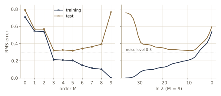
The best test error comes from a moderate \(\lambda\). Of course, we cannot choose \(\lambda\) or \(M\) by looking at the test set, or it stops being a test set. Section Model selection shows how to choose them from the training data alone.
Probability theory
The noise in the targets is the reason curve fitting is hard: with a finite, noisy data set there is uncertainty about the right curve. Probability theory gives us a consistent language for that uncertainty, and combined with decision theory it lets us make the best predictions possible from the information we have.
The sum and product rules
Consider two discrete random variables: \(X\) takes values \(x_1, \dots, x_I\) and \(Y\) takes values \(y_1, \dots, y_J\). Suppose we observe \(N\) joint trials and let \(n_{ij}\) be the number in which \(X = x_i\) and \(Y = y_j\), with row totals \(c_i = \sum_j n_{ij}\). In the limit of many trials, the fractions become probabilities:
- the joint probability \(p(X = x_i, Y = y_j) = n_{ij}/N\);
- the marginal probability \(p(X = x_i) = c_i/N\);
- the conditional probability \(p(Y = y_j \mid X = x_i) = n_{ij}/c_i\), the fraction of trials with \(X = x_i\) that also have \(Y = y_j\).
Since \(c_i = \sum_j n_{ij}\) and \(n_{ij}/N = (n_{ij}/c_i)(c_i/N)\), these satisfy the two rules on which all of probability theory rests. Writing \(p(X)\) for the distribution over all values of \(X\), they are the sum rule and the product rule:
\[p(X) = \sum_{Y} p(X, Y), \qquad\qquad p(X, Y) = p(Y \mid X)\, p(X).\]Here is a joint distribution over \(X \in \{0, 1, 2\}\) and \(Y \in \{0, 1\}\), the frequencies from 20,000 simulated trials, and both rules at work.
P_XY = np.array([[0.10, 0.25],          # rows: X = 0, 1, 2; columns: Y = 0, 1
                 [0.20, 0.15],
                 [0.05, 0.25]])
draws = rng.choice(6, size=20_000, p=P_XY.ravel())
counts = np.bincount(draws, minlength=6).reshape(3, 2)      # n_ij

p_X = P_XY.sum(axis=1)                                      # sum rule
p_Y_given_X = P_XY / p_X[:, None]                           # product rule, rearranged
print("counts n_ij:\n", counts)
print("p(X) exact:", p_X, "  from counts:", counts.sum(axis=1) / counts.sum())
print("p(Y=1 | X) exact:", p_Y_given_X[:, 1],
      "  from counts:", counts[:, 1] / counts.sum(axis=1))
print("product rule rebuilds the joint:", np.allclose(p_Y_given_X * p_X[:, None], P_XY))
counts n_ij:
 [[2032 4969]
 [4031 2979]
 [ 992 4997]]
p(X) exact: [0.35 0.35 0.3 ]   from counts: [0.35   0.3505 0.2994]
p(Y=1 | X) exact: [0.7143 0.4286 0.8333]   from counts: [0.7098 0.425  0.8344]
product rule rebuilds the joint: True
The frequencies approach the probabilities as the number of trials grows, and the product rule rebuilds the joint table from a marginal and a conditional.
Bayes’ theorem
The product rule can be applied in either order, \(p(X, Y) = p(Y \mid X)p(X) = p(X \mid Y)p(Y)\). Dividing by \(p(X)\) gives
Result. Bayes’ theorem: \(p(Y \mid X) = \dfrac{p(X \mid Y)\, p(Y)}{p(X)}\), where \(p(X) = \sum_{Y} p(X \mid Y)\, p(Y)\).
The denominator, obtained from the sum rule, is a normalizing constant that makes the left side sum to one over \(Y\). The theorem turns a probability we know how to specify, \(X\) given \(Y\), into one we want, \(Y\) given \(X\).
A small example. Suppose 20% of the email arriving at a mailbox is spam. The word “prize” appears in 40% of spam messages but only 1% of legitimate ones. A message arrives containing “prize”. How likely is it to be spam? Before reading the message, our prior probability of spam is \(p(\text{spam}) = 0.2\). After seeing the word, the posterior probability is
\[p(\text{spam} \mid \text{prize}) = \frac{0.4 \times 0.2}{0.4 \times 0.2 + 0.01 \times 0.8} = \frac{0.08}{0.088} \approx 0.909.\]Let us check it by simulating a million emails.
p_spam, p_word_spam, p_word_ham = 0.2, 0.40, 0.01
posterior = p_word_spam * p_spam / (p_word_spam * p_spam + p_word_ham * (1 - p_spam))

sim = np.random.default_rng(1)
is_spam = sim.random(1_000_000) < p_spam
has_word = sim.random(1_000_000) < np.where(is_spam, p_word_spam, p_word_ham)
print(f"Bayes' theorem: {posterior:.4f}   simulation: {is_spam[has_word].mean():.4f}")
print(f"fraction of email with the word: {has_word.mean():.4f}   (p(prize) = 0.088)")
Bayes' theorem: 0.9091   simulation: 0.9082
fraction of email with the word: 0.0882   (p(prize) = 0.088)
One word moved us from 20% to about 91%. Notice that the posterior depends on the prior: if only 1% of email were spam, the same word would give a posterior of only about 29%. Mixing up \(p(\text{prize} \mid \text{spam})\) with \(p(\text{spam} \mid \text{prize})\) is one of the most common errors in reasoning with probabilities.
Two variables are independent if their joint distribution factorizes, \(p(X, Y) = p(X)p(Y)\); then \(p(Y \mid X) = p(Y)\), and observing \(X\) tells us nothing about \(Y\). In the table above, \(p(Y = 1 \mid X)\) changes with \(X\), so those variables are dependent.
Probability densities
For a continuous variable \(x\), the probability that \(x\) falls in a small interval \((x, x + \delta x)\) is \(p(x)\,\delta x\) for small \(\delta x\); the function \(p(x)\) is the probability density. It satisfies \(p(x) \ge 0\) and \(\int p(x)\,dx = 1\), and the probability of an interval is \(\int_a^b p(x)\,dx\). The cumulative distribution function is \(P(z) = \int_{-\infty}^{z} p(x)\,dx\), with \(P'(x) = p(x)\). A density can exceed 1; only its integrals are probabilities. For a vector \(\mathbf{x}\) the definitions are the same with multiple integrals, and the sum and product rules become
\[p(x) = \int p(x, y)\, dy, \qquad p(x, y) = p(y \mid x)\, p(x).\]Densities behave differently from ordinary functions when we change variables. Suppose \(x = g(y)\) for a monotonic function \(g\). The probability in a small interval must be the same whichever variable we use, so \(p_y(y)\,\lvert \delta y \rvert = p_x(x)\,\lvert \delta x \rvert\), which gives
\[p_y(y) = p_x\bigl(g(y)\bigr)\, \lvert g'(y) \rvert .\]The factor \(\lvert g'(y) \rvert\), the Jacobian of the transformation, stretches or compresses the density. One consequence surprises many people: the location of the maximum of a density depends on the choice of variable. A function \(f(x)\) has its maximum at the same point whether we write it in terms of \(x\) or of \(y\), but the Jacobian factor can move the maximum of a density.
Here is a clean example. Let \(x\) be Gaussian with mean \(\mu = 1\) and standard deviation \(\sigma = 0.6\), and let \(y = e^{x}\), so \(x = g(y) = \ln y\) and \(g'(y) = 1/y\). The mode of \(p_x\) is at \(x = \mu\), which maps to \(y = e^{\mu} \approx 2.718\). But \(p_y(y) = p_x(\ln y)/y\), and setting the derivative of \(\ln p_y(y) = -(\ln y - \mu)^2/(2\sigma^2) - \ln y + \text{const}\) to zero gives the mode \(y = e^{\mu - \sigma^2} \approx 1.896\). The code confirms this on a fine grid, and checks the transformed density against a histogram of samples.
def gauss_pdf(x, mu, var):
    """Univariate Gaussian density N(x | mu, var)."""
    return np.exp(-0.5 * (x - mu) ** 2 / var) / np.sqrt(2 * np.pi * var)

mu, sd = 1.0, 0.6
y_grid = np.linspace(1e-3, 40, 400_001)
p_y = gauss_pdf(np.log(y_grid), mu, sd ** 2) / y_grid     # p_x(g(y)) |g'(y)|, g = ln
print(f"integral of p_y: {np.trapezoid(p_y, y_grid):.5f}")
print(f"g^-1(mode of p_x) = e^mu        = {np.exp(mu):.4f}")
print(f"mode of p_y on the grid          = {y_grid[np.argmax(p_y)]:.4f}")
print(f"mode of p_y from calculus e^(mu - sigma^2) = {np.exp(mu - sd ** 2):.4f}")

y_samples = np.exp(rng.normal(mu, sd, 200_000))
dens, edges = np.histogram(y_samples, bins=60, range=(0, 8), density=True)
mids = (edges[:-1] + edges[1:]) / 2
dens *= (y_samples < 8).mean()                            # histogram covers only [0, 8)
p_mid = gauss_pdf(np.log(mids), mu, sd ** 2) / mids
print(f"largest gap between histogram and formula: {np.abs(dens - p_mid).max():.4f}"
      f"  (peak {p_mid.max():.3f})")
integral of p_y: 1.00000
g^-1(mode of p_x) = e^mu        = 2.7183
mode of p_y on the grid          = 1.8965
mode of p_y from calculus e^(mu - sigma^2) = 1.8965
largest gap between histogram and formula: 0.0053  (peak 0.293)
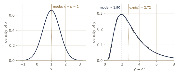
This matters in machine learning because we often maximize densities, for instance when we choose the single most probable parameter value. The answer depends on how we parameterize the model.
Expectations and covariances
The expectation of a function \(f\) under a distribution \(p\) is its average value, weighted by probability:
\[\mathbb{E}[f] = \sum_x p(x) f(x) \quad\text{(discrete)}, \qquad \mathbb{E}[f] = \int p(x) f(x)\, dx \quad\text{(continuous)}.\]If we have \(N\) points drawn independently from \(p\), the sample average approximates the expectation, and the approximation becomes exact as \(N \to \infty\):
\[\mathbb{E}[f] \approx \frac{1}{N} \sum_{n=1}^{N} f(x_n).\]This is the simplest Monte Carlo estimate, and sampling methods of this kind get a whole module (module 11). With several variables we write \(\mathbb{E}_x[f(x, y)]\) to say which variable is averaged over (the result is a function of \(y\)), and the conditional expectation \(\mathbb{E}_x[f \mid y] = \sum_x p(x \mid y) f(x)\) averages under a conditional distribution.
The variance measures how much \(f\) varies around its mean,
\[\operatorname{var}[f] = \mathbb{E}\bigl[(f(x) - \mathbb{E}[f(x)])^2\bigr] = \mathbb{E}[f(x)^2] - \mathbb{E}[f(x)]^2 ,\]and the covariance of two variables measures how much they vary together, \(\operatorname{cov}[x, y] = \mathbb{E}_{x,y}[xy] - \mathbb{E}[x]\mathbb{E}[y]\). It is zero for independent variables. For vectors \(\mathbf{x}\) and \(\mathbf{y}\) the covariance is a matrix,
\[\operatorname{cov}[\mathbf{x}, \mathbf{y}] = \mathbb{E}_{\mathbf{x},\mathbf{y}}\bigl[ (\mathbf{x} - \mathbb{E}[\mathbf{x}])(\mathbf{y}^{\mathrm{T}} - \mathbb{E}[\mathbf{y}^{\mathrm{T}}]) \bigr],\]and we write \(\operatorname{cov}[\mathbf{x}] \equiv \operatorname{cov}[\mathbf{x}, \mathbf{x}]\) for the covariance matrix of the components of \(\mathbf{x}\) with each other. For the log-normal variable \(y = e^{x}\) above, \(\mathbb{E}[y] = e^{\mu + \sigma^2/2}\) and \(\operatorname{var}[y] = (e^{\sigma^2} - 1)e^{2\mu + \sigma^2}\) in closed form. Let us watch the Monte Carlo estimates converge to them, and check a sample covariance matrix.
E_y = np.exp(mu + sd ** 2 / 2)
var_y = (np.exp(sd ** 2) - 1) * np.exp(2 * mu + sd ** 2)
for N in [10, 1_000, 100_000]:
    ys = y_samples[:N]
    print(f"N = {N:>7}:  mean {ys.mean():.4f} (exact {E_y:.4f})   "
          f"variance {ys.var():.4f} (exact {var_y:.4f})")

Sigma = np.array([[1.0, 0.8], [0.8, 2.0]])
L = np.linalg.cholesky(Sigma)
X2 = rng.normal(size=(50_000, 2)) @ L.T        # rows: samples with covariance L L^T
Xc = X2 - X2.mean(axis=0)
print("sample covariance:\n", Xc.T @ Xc / len(X2))
N =      10:  mean 3.8499 (exact 3.2544)   variance 5.4863 (exact 4.5894)
N =    1000:  mean 3.1800 (exact 3.2544)   variance 4.3313 (exact 4.5894)
N =  100000:  mean 3.2466 (exact 3.2544)   variance 4.5297 (exact 4.5894)
sample covariance:
 [[1.0041 0.8024]
 [0.8024 1.9993]]
The error of a Monte Carlo average shrinks like \(1/\sqrt{N}\): a hundred times more samples buys one more correct digit.
Bayesian probabilities
So far probabilities were frequencies of repeatable events. That is the frequentist interpretation. The Bayesian interpretation is broader: a probability measures a degree of belief about anything uncertain, including things that happen only once, such as the value of a physical constant or the right coefficients for our polynomial. It can be shown that any consistent system for manipulating degrees of belief, under a few common-sense requirements, must obey the sum and product rules (Bishop §1.2.3 gives references), so it is natural to call these beliefs probabilities.
For curve fitting, the Bayesian view lets us treat the coefficients \(\mathbf{w}\) as uncertain. We state our assumptions about them before seeing data in a prior \(p(\mathbf{w})\). The observed targets \(\mathcal{D} = \{t_1, \dots, t_N\}\) enter through \(p(\mathcal{D} \mid \mathbf{w})\), and Bayes’ theorem gives the posterior:
\[p(\mathbf{w} \mid \mathcal{D}) = \frac{p(\mathcal{D} \mid \mathbf{w})\, p(\mathbf{w})}{p(\mathcal{D})}, \qquad p(\mathcal{D}) = \int p(\mathcal{D} \mid \mathbf{w})\, p(\mathbf{w})\, d\mathbf{w}.\]Definition. Viewed as a function of \(\mathbf{w}\) for the observed data, \(p(\mathcal{D} \mid \mathbf{w})\) is called the likelihood function. It is not a probability distribution over \(\mathbf{w}\) and need not integrate to one over \(\mathbf{w}\). In words, posterior ∝ likelihood × prior.
Both schools use the likelihood, but differently. A frequentist treats \(\mathbf{w}\) as a fixed unknown and computes an estimator from the data. The most common one is maximum likelihood, which chooses the \(\mathbf{w}\) that makes the observed data most probable. (The negative log-likelihood is often called an error function; maximizing the likelihood minimizes the error.) Uncertainty in the estimate is then described by how the estimate would vary over hypothetical repeated data sets. One practical way to imitate repeated data sets is the bootstrap: create \(L\) new data sets of size \(N\) by drawing \(N\) points with replacement from the original one, recompute the estimate on each, and look at the spread. A Bayesian instead conditions on the one data set actually observed and expresses the uncertainty in \(\mathbf{w}\) through the posterior.
Here is the bootstrap for the mean of 40 log-normal values. For the mean we also know the usual standard error \(s/\sqrt{N}\), which gives a check; for the median no such simple formula exists, and the bootstrap still works.
data40 = y_samples[-40:]
boot = np.random.default_rng(2)
L_boot = 5_000
idx = boot.integers(0, 40, size=(L_boot, 40))           # each row: one resampled data set
boot_means = data40[idx].mean(axis=1)
boot_medians = np.median(data40[idx], axis=1)
print(f"sample mean {data40.mean():.3f}:  bootstrap s.e. {boot_means.std():.3f}   "
      f"s/sqrt(N) = {data40.std(ddof=1) / np.sqrt(40):.3f}")
print(f"sample median {np.median(data40):.3f}:  bootstrap s.e. {boot_medians.std():.3f}")
sample mean 3.416:  bootstrap s.e. 0.377   s/sqrt(N) = 0.382
sample median 2.688:  bootstrap s.e. 0.288
The bootstrap standard error of the mean, 0.377, agrees closely with the formula’s 0.382. For the median, which has no such simple formula, the same few lines give 0.288.
A strength of the Bayesian view is that prior knowledge enters naturally. If a coin that looks fair lands heads three times out of three, maximum likelihood estimates the probability of heads as 1, predicting heads forever. Any sensible prior that puts most of its weight near 0.5 pulls the estimate back toward the middle; module 02 does this with the beta distribution. The usual criticism is the other side of the same coin: conclusions depend on the prior, which is sometimes chosen for convenience rather than conviction. The full Bayesian recipe also requires sums or integrals over all parameter values, which were long impractical; sampling methods (module 11) and deterministic approximations (module 10) are what made it usable. This course uses both viewpoints, leaning Bayesian as the book does.
The Gaussian distribution
The most important distribution for continuous variables is the Gaussian or normal distribution. For a single variable,
\[\mathcal{N}(x \mid \mu, \sigma^2) = \frac{1}{(2\pi\sigma^2)^{1/2}} \exp\left\{ -\frac{1}{2\sigma^2}(x - \mu)^2 \right\}.\]Its two parameters are the mean \(\mu\) and the variance \(\sigma^2\); \(\sigma\) is the standard deviation and \(\beta = 1/\sigma^2\) the precision. It is normalized, \(\mathbb{E}[x] = \mu\), \(\mathbb{E}[x^2] = \mu^2 + \sigma^2\), and \(\operatorname{var}[x] = \sigma^2\); the maximum (the mode) is at \(x = \mu\). For a \(D\)-dimensional vector,
\[\mathcal{N}(\mathbf{x} \mid \boldsymbol{\mu}, \boldsymbol{\Sigma}) = \frac{1}{(2\pi)^{D/2}\, \lvert \boldsymbol{\Sigma} \rvert^{1/2}} \exp\left\{ -\frac12 (\mathbf{x} - \boldsymbol{\mu})^{\mathrm{T}} \boldsymbol{\Sigma}^{-1} (\mathbf{x} - \boldsymbol{\mu}) \right\},\]with mean vector \(\boldsymbol{\mu}\) and \(D \times D\) covariance matrix \(\boldsymbol{\Sigma}\). Module 02 studies it in depth. A quick numerical check of the one-dimensional facts:
xs = np.linspace(-10, 12, 200_001)
p = gauss_pdf(xs, 1.5, 0.7 ** 2)
print(f"integral {np.trapezoid(p, xs):.6f}   E[x] {np.trapezoid(xs * p, xs):.6f}   "
      f"var[x] {np.trapezoid((xs - 1.5) ** 2 * p, xs):.6f}   (sigma^2 = {0.7 ** 2:.2f})")
integral 1.000000 E[x] 1.500000 var[x] 0.490000 (sigma^2 = 0.49)
Maximum likelihood for a Gaussian. Suppose \(\mathbf{x} = (x_1, \dots, x_N)^{\mathrm{T}}\) are drawn independently and identically distributed (i.i.d.) from a Gaussian with unknown \(\mu\) and \(\sigma^2\). Independence means the joint probability is a product, so the likelihood is
\[p(\mathbf{x} \mid \mu, \sigma^2) = \prod_{n=1}^{N} \mathcal{N}(x_n \mid \mu, \sigma^2).\]Products of many small numbers underflow, and logs turn products into sums, so we maximize the log-likelihood instead, which has the same maximizer because \(\ln\) is increasing:
\[\ln p(\mathbf{x} \mid \mu, \sigma^2) = -\frac{1}{2\sigma^2} \sum_{n=1}^{N} (x_n - \mu)^2 - \frac{N}{2} \ln \sigma^2 - \frac{N}{2} \ln(2\pi).\]The derivative with respect to \(\mu\) vanishes when \(\sum_n (x_n - \mu) = 0\), and the derivative with respect to \(\sigma^2\) vanishes when \(\frac{1}{2\sigma^4}\sum_n (x_n - \mu)^2 - \frac{N}{2\sigma^2} = 0\). Solving these gives
\[\mu_{\mathrm{ML}} = \frac{1}{N} \sum_{n=1}^{N} x_n , \qquad \sigma^2_{\mathrm{ML}} = \frac{1}{N} \sum_{n=1}^{N} (x_n - \mu_{\mathrm{ML}})^2 ,\]the sample mean and the sample variance about the sample mean. (Because the \(\mu\) equation does not involve \(\sigma^2\), we can solve for \(\mu\) first and then plug it in.)
These estimates have a systematic flaw. Averaging over data sets, using \(\mathbb{E}[x_n x_m] = \mu^2 + \sigma^2 \delta_{nm}\) for independent draws, one finds
\[\mathbb{E}[\mu_{\mathrm{ML}}] = \mu, \qquad \mathbb{E}[\sigma^2_{\mathrm{ML}}] = \frac{N-1}{N} \sigma^2 .\]To see where the factor comes from: \(\sum_n (x_n - \mu_{\mathrm{ML}})^2 = \sum_n (x_n - \mu)^2 - N(\mu_{\mathrm{ML}} - \mu)^2\), and the expectations of the two terms are \(N\sigma^2\) and \(N \operatorname{var}[\mu_{\mathrm{ML}}] = N \cdot \sigma^2/N = \sigma^2\). So the ML variance underestimates the true variance on average: it is a biased estimator. The reason is that it measures spread around the sample mean, which was fitted to the same data and is therefore closer to the points than the true mean. Multiplying by \(N/(N-1)\) removes the bias. A simulation with tiny data sets of size 5 makes the effect plain:
mu_true, var_true, N = 1.5, 0.49, 5
sim3 = np.random.default_rng(3)
sets = sim3.normal(mu_true, np.sqrt(var_true), size=(200_000, N))   # 200,000 data sets
mu_ml = sets.mean(axis=1)
var_ml = ((sets - mu_ml[:, None]) ** 2).mean(axis=1)
print(f"average mu_ML     = {mu_ml.mean():.4f}   (true mu = {mu_true})")
print(f"average sigma2_ML = {var_ml.mean():.4f}   "
      f"((N-1)/N sigma^2 = {(N - 1) / N * var_true:.4f}, sigma^2 = {var_true})")
print(f"average of N/(N-1) sigma2_ML = {(N / (N - 1) * var_ml).mean():.4f}")
average mu_ML     = 1.5004   (true mu = 1.5)
average sigma2_ML = 0.3922   ((N-1)/N sigma^2 = 0.3920, sigma^2 = 0.49)
average of N/(N-1) sigma2_ML = 0.4902
Note. The bias vanishes as \(N \to \infty\), so for a single Gaussian it rarely matters. But it is the simplest example of a general fact: maximum likelihood fits the noise in the training data, and the more parameters the model has, the stronger the effect. It is the same phenomenon as overfitting in curve fitting, where the order-9 polynomial reported zero training error.
Curve fitting revisited: maximum likelihood and MAP
Now we put the curve-fitting problem into probabilistic form. Assume that, given \(x\), the target is Gaussian with mean \(y(x, \mathbf{w})\) and precision \(\beta\):
\[p(t \mid x, \mathbf{w}, \beta) = \mathcal{N}\bigl(t \mid y(x, \mathbf{w}), \beta^{-1}\bigr).\]For i.i.d. data the log-likelihood is
\[\ln p(\mathbf{t} \mid \mathbf{x}, \mathbf{w}, \beta) = -\frac{\beta}{2} \sum_{n=1}^{N} \bigl( y(x_n, \mathbf{w}) - t_n \bigr)^2 + \frac{N}{2} \ln \beta - \frac{N}{2} \ln(2\pi).\]The last two terms do not involve \(\mathbf{w}\), and the factor \(\beta\) in front of the sum does not change where the maximum is. So maximizing the likelihood over \(\mathbf{w}\) is exactly minimizing the sum-of-squares error \(E(\mathbf{w})\): least squares is maximum likelihood under Gaussian noise, and \(\mathbf{w}_{\mathrm{ML}} = \mathbf{w}^\star\). Maximizing then over \(\beta\) gives
\[\frac{1}{\beta_{\mathrm{ML}}} = \frac{1}{N} \sum_{n=1}^{N} \bigl( y(x_n, \mathbf{w}_{\mathrm{ML}}) - t_n \bigr)^2 ,\]the mean squared residual. We now have a predictive distribution, not just a point prediction: \(p(t \mid x, \mathbf{w}_{\mathrm{ML}}, \beta_{\mathrm{ML}}) = \mathcal{N}(t \mid y(x, \mathbf{w}_{\mathrm{ML}}), \beta_{\mathrm{ML}}^{-1})\). If the model is right, about 95% of new targets should land within two standard deviations of the curve.
def log_likelihood(w, beta, x, t):
    """ln p(t | x, w, beta) for the Gaussian noise model."""
    r = predict(w, x) - t
    N = len(t)
    return -0.5 * beta * r @ r + 0.5 * N * np.log(beta) - 0.5 * N * np.log(2 * np.pi)

for M in [3, 9]:
    w_ml = fit_poly(x, t, M)
    beta_ml = 1 / np.mean((predict(w_ml, x) - t) ** 2)
    inside = np.abs(t_test - predict(w_ml, x_test)) < 2 / np.sqrt(beta_ml)
    print(f"M = {M}:  noise s.d. 1/sqrt(beta_ML) = {1 / np.sqrt(beta_ml):.2e}   "
          f"test targets within 2 s.d.: {inside.mean():.1%}")

# finite-difference check that w_ML maximizes the log-likelihood (M = 3)
beta3 = 1 / np.mean((predict(w3, x) - t) ** 2)
h = 1e-6
grad = [(log_likelihood(w3 + h * e, beta3, x, t)
         - log_likelihood(w3 - h * e, beta3, x, t)) / (2 * h) for e in np.eye(4)]
print("d lnp / dw at w_ML (M=3):", np.array(grad))
M = 3:  noise s.d. 1/sqrt(beta_ML) = 2.13e-01   test targets within 2 s.d.: 82.6%
M = 9:  noise s.d. 1/sqrt(beta_ML) = 2.39e-11   test targets within 2 s.d.: 0.0%
d lnp / dw at w_ML (M=3): [ 0. -0.  0. -0.]
For \(M = 3\), the estimated noise level (0.21) is well below the true 0.3, as the bias result leads us to expect, and the predictive distribution covers only about 83% of the test targets instead of 95%. For \(M = 9\) the training residuals are all zero, so maximum likelihood concludes that there is no noise at all (\(\beta_{\mathrm{ML}}\) is infinite up to rounding) and its error bars exclude nearly every test point. That is overfitting in its most extreme form.
MAP estimation. Now take a step toward Bayes. Put a Gaussian prior on the coefficients, centered at zero with precision \(\alpha\):
\[p(\mathbf{w} \mid \alpha) = \mathcal{N}(\mathbf{w} \mid \mathbf{0}, \alpha^{-1}\mathbf{I}) = \left( \frac{\alpha}{2\pi} \right)^{(M+1)/2} \exp\left\{ -\frac{\alpha}{2} \mathbf{w}^{\mathrm{T}}\mathbf{w} \right\}.\]Such a parameter of the prior is called a hyperparameter. The posterior is proportional to likelihood times prior, and the \(\mathbf{w}\) that maximizes it is the maximum a posteriori or MAP estimate. Taking the negative log of the posterior and dropping terms that do not depend on \(\mathbf{w}\), we must minimize
\[\frac{\beta}{2} \sum_{n=1}^{N} \bigl( y(x_n, \mathbf{w}) - t_n \bigr)^2 + \frac{\alpha}{2} \mathbf{w}^{\mathrm{T}}\mathbf{w}.\]Dividing by \(\beta\) gives exactly the regularized error \(\widetilde{E}(\mathbf{w})\) with \(\lambda = \alpha / \beta\). So ridge regression is MAP estimation with a Gaussian prior, and the regularizer we added by hand is the prior belief that the coefficients are probably small. Let us check the equivalence by computing the gradient of the negative log posterior at the ridge solution.
alpha, beta = 5e-3, 1 / 0.3 ** 2      # prior precision; the true noise precision
w_map = fit_poly(x, t, 9, lam=alpha / beta)
Phi9 = design_matrix(x, 9)
grad_neg_log_post = beta * Phi9.T @ (Phi9 @ w_map - t) + alpha * w_map
print(f"lambda = alpha/beta = {alpha / beta:.1e}   (ln lambda = {np.log(alpha / beta):.2f})")
print(f"|gradient of -ln posterior| at the ridge solution: "
      f"{np.linalg.norm(grad_neg_log_post):.1e}")
print(f"MAP fit, M = 9:  test E_RMS = {rms_error(w_map, x_test, t_test):.3f}")
lambda = alpha/beta = 4.5e-04   (ln lambda = -7.71)
|gradient of -ln posterior| at the ridge solution: 9.1e-14
MAP fit, M = 9:  test E_RMS = 0.320
Bayesian curve fitting
MAP still returns a single \(\mathbf{w}\). A fully Bayesian treatment keeps the whole posterior and averages the predictions of every \(\mathbf{w}\), weighted by how plausible it is. Treating \(\alpha\) and \(\beta\) as known for now, the predictive distribution for a new input \(x\) is obtained with the sum and product rules:
\[p(t \mid x, \mathbf{x}, \mathbf{t}) = \int p(t \mid x, \mathbf{w})\, p(\mathbf{w} \mid \mathbf{x}, \mathbf{t})\, d\mathbf{w}.\]For our model, the posterior over \(\mathbf{w}\) is Gaussian and the integral can be done in closed form. The result, derived in module 03, is again a Gaussian, \(p(t \mid x, \mathbf{x}, \mathbf{t}) = \mathcal{N}\bigl(t \mid m(x), s^2(x)\bigr)\), with
\[m(x) = \beta\, \boldsymbol{\phi}(x)^{\mathrm{T}} \mathbf{S} \sum_{n=1}^{N} \boldsymbol{\phi}(x_n)\, t_n, \qquad s^2(x) = \beta^{-1} + \boldsymbol{\phi}(x)^{\mathrm{T}} \mathbf{S}\, \boldsymbol{\phi}(x), \qquad \mathbf{S}^{-1} = \alpha \mathbf{I} + \beta \sum_{n=1}^{N} \boldsymbol{\phi}(x_n) \boldsymbol{\phi}(x_n)^{\mathrm{T}},\]where \(\boldsymbol{\phi}(x) = (1, x, \dots, x^M)^{\mathrm{T}}\) is the vector of powers, so the \(\boldsymbol{\phi}(x_n)^{\mathrm{T}}\) are the rows of \(\mathbf{\Phi}\). Two things to notice. The mean \(m(x)\) equals the MAP prediction (compare the formula with the ridge solution). And the variance has two parts: \(\beta^{-1}\) is the noise on the targets, and \(\boldsymbol{\phi}^{\mathrm{T}}\mathbf{S}\boldsymbol{\phi}\) is our remaining uncertainty about \(\mathbf{w}\), which depends on \(x\).
def bayes_poly_predictive(x_new, x, t, M, alpha, beta):
    """Mean m(x) and variance s^2(x) of the Bayesian predictive distribution."""
    Phi = design_matrix(x, M)
    S_inv = alpha * np.eye(M + 1) + beta * Phi.T @ Phi
    phi = design_matrix(np.atleast_1d(x_new), M)
    m = beta * phi @ np.linalg.solve(S_inv, Phi.T @ t)
    s2 = 1 / beta + np.sum(phi * np.linalg.solve(S_inv, phi.T).T, axis=1)
    return m, s2

x_new = np.array([0.0, 0.25, 0.5, 0.9, 1.1])
m, s2 = bayes_poly_predictive(x_new, x, t, 9, alpha, beta)
for xv, mv, sv in zip(x_new, m, np.sqrt(s2)):
    print(f"x = {xv:4.2f}:  m(x) = {mv:7.3f}   s(x) = {sv:.3f}   "
          f"sin(2 pi x) = {np.sin(2 * np.pi * xv):6.3f}")
print(f"m(x) equals the MAP prediction: {np.allclose(m, predict(w_map, x_new))}")
m_t, s2_t = bayes_poly_predictive(x_test, x, t, 9, alpha, beta)
inside = np.abs(t_test - m_t) < 2 * np.sqrt(s2_t)
print(f"test targets within 2 s(x): {inside.mean():.1%}")
x = 0.00:  m(x) =   0.295   s(x) = 0.401   sin(2 pi x) =  0.000
x = 0.25:  m(x) =   0.912   s(x) = 0.348   sin(2 pi x) =  1.000
x = 0.50:  m(x) =   0.001   s(x) = 0.344   sin(2 pi x) =  0.000
x = 0.90:  m(x) =  -0.578   s(x) = 0.394   sin(2 pi x) = -0.588
x = 1.10:  m(x) =   0.588   s(x) = 2.003   sin(2 pi x) =  0.588
m(x) equals the MAP prediction: True
test targets within 2 s(x): 96.9%
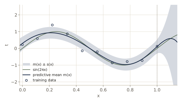
The error bars now do their job: the fraction of test targets within two predictive standard deviations is close to the nominal 95%, and the band widens where there is no data. We still fixed \(\alpha\) and \(\beta\) by hand; module 03 shows how to set them from the training data alone, and how the same machinery compares models of different orders.
Model selection
We have seen that the order \(M\) or the penalty \(\lambda\) sets how flexible the fitted model can be, and that the training error is useless for choosing them: it always favors the most complex option. Choosing among such settings is model selection.
Validation sets and cross-validation
If data are plentiful, we can hold some back. Train each candidate model on the training set, compare them on a separate validation set, and pick the best. If we try many candidates, we can overfit the validation set too, so a third, untouched test set is kept for the final estimate of performance.
Often data are scarce and we want to train on as much as possible. S-fold cross-validation reuses the data: split it into \(S\) groups of about equal size, train on \(S - 1\) groups and evaluate on the remaining one, repeat for each of the \(S\) choices of held-out group, and average the \(S\) scores. The extreme case \(S = N\) is leave-one-out cross-validation. Let us implement it and choose \(M\) (without regularization) and \(\lambda\) (for \(M = 9\)) on a new data set of 30 points with random inputs.
def kfold_indices(N, S, rng):
    """Split a random permutation of 0..N-1 into S nearly equal folds."""
    return np.array_split(rng.permutation(N), S)

def cv_rms(x, t, S, rng, M, lam=0.0):
    """S-fold cross-validation estimate of E_RMS (order M, penalty lam)."""
    folds = kfold_indices(len(x), S, rng)
    sq_err = 0.0
    for k in range(S):
        hold = folds[k]
        train = np.concatenate([folds[j] for j in range(S) if j != k])
        w = fit_poly(x[train], t[train], M, lam)
        sq_err += np.sum((predict(w, x[hold]) - t[hold]) ** 2)
    return np.sqrt(sq_err / len(x))

x30, t30 = make_data(30, rng, random_x=True)
print(" M   5-fold CV   test (trained on all 30)")
for M in range(10):
    cv = cv_rms(x30, t30, 5, np.random.default_rng(10), M)   # same folds for every M
    test = rms_error(fit_poly(x30, t30, M), x_test, t_test)
    print(f"{M:2d}   {cv:9.3f}   {test:.3f}")
 M   5-fold CV   test (trained on all 30)
 0       0.850   0.801
 1       0.537   0.559
 2       0.570   0.559
 3       0.289   0.329
 4       0.306   0.333
 5       0.322   0.347
 6       0.307   0.417
 7       0.311   0.376
 8       0.334   0.340
 9       0.364   0.567
Using the same folds for every candidate (the seeded generator in the loop) makes the comparison fair: differences between rows come from the models, not from different random splits. Cross-validation picks \(M = 3\), which also has the lowest test error. For the largest orders it is too optimistic, but it ranks the models sensibly, and it never looked at the test set. Now the penalty for \(M = 9\):
grid = np.arange(-25, 1, 1.0)
cv_l = [cv_rms(x30, t30, 5, np.random.default_rng(10), 9, np.exp(a)) for a in grid]
a_best = grid[np.argmin(cv_l)]
w_cv = fit_poly(x30, t30, 9, np.exp(a_best))
print(f"5-fold CV picks ln lambda = {a_best:.0f} (CV E_RMS {min(cv_l):.3f})")
print(f"test E_RMS of the refit on all 30 points: {rms_error(w_cv, x_test, t_test):.3f}")

loo = [cv_rms(x, t, 10, np.random.default_rng(10), M) for M in range(9)]
print("leave-one-out on the original 10 points, M = 0..8:", np.round(loo, 3))
5-fold CV picks ln lambda = -9 (CV E_RMS 0.303)
test E_RMS of the refit on all 30 points: 0.319
leave-one-out on the original 10 points, M = 0..8: [ 0.789  0.708  0.959  0.32   0.611  1.585  2.11   4.099 32.072]
On the ten-point set, leave-one-out also rejects the very low and the very high orders. (We stop at \(M = 8\) because each leave-one-out fit sees only nine points.)
In practice. Cross-validation multiplies the training cost by \(S\), and with several complexity parameters the number of combinations to try grows exponentially. Always refit the chosen model on all the data at the end, and report its performance on data that played no part in any choice.
Information criteria
An alternative is to correct the training log-likelihood for its optimism with a penalty that grows with the number of parameters, and choose the model with the best corrected score. The Akaike information criterion (AIC) picks the model that maximizes
\[\ln p(\mathcal{D} \mid \mathbf{w}_{\mathrm{ML}}) - P,\]where \(P\) is the number of adjustable parameters. The Bayesian information criterion (BIC) uses the larger penalty \(\tfrac12 P \ln N\); it comes from an approximation to Bayesian model comparison and is derived in module 04 (Bishop §4.4.1). For our polynomial with a fitted noise precision, \(P = M + 2\).
print(" M    ln p(D|w_ML)    AIC      BIC")
for M in range(10):
    w = fit_poly(x30, t30, M)
    b = 1 / np.mean((predict(w, x30) - t30) ** 2)
    ll = log_likelihood(w, b, x30, t30)
    P = M + 2
    print(f"{M:2d}   {ll:10.2f}   {ll - P:7.2f}   {ll - 0.5 * P * np.log(30):7.2f}")
 M    ln p(D|w_ML)    AIC      BIC
 0       -37.39    -39.39    -40.79
 1       -21.57    -24.57    -26.67
 2       -21.55    -25.55    -28.35
 3        -1.99     -6.99    -10.49
 4        -1.17     -7.17    -11.37
 5        -1.06     -8.06    -12.96
 6        -0.21     -8.21    -13.82
 7        -0.09     -9.09    -15.40
 8         0.01     -9.99    -16.99
 9         1.27     -9.73    -17.44
The log-likelihood keeps rising with \(M\), but both criteria peak at a moderate order. These criteria are cheap because they need only one fit per model, but they ignore the uncertainty in the parameters and tend to favor models that are too simple. The fully Bayesian treatment of model comparison in module 03 (Bishop §3.4) does better, and complexity penalties arise from it naturally.
The curse of dimensionality
Our example had one input. Real problems have many: pixels, sensor channels, words. Some ideas that work well in one or two dimensions fail badly in many, and this is known as the curse of dimensionality.
Methods that grow exponentially
Consider a naive classifier. Divide the input space into a grid of cells; to classify a new point, find its cell and take a majority vote of the training points in that cell. With \(k\) divisions per axis and \(D\) inputs there are \(k^D\) cells, and each cell needs training points in it. Polynomials suffer in a similar way: a general polynomial of order \(M\) in \(D\) variables has \(\binom{D + M}{M}\) coefficients (count the monomials of degree at most \(M\)), which grows like \(D^M\).
from math import comb
print("    D   grid cells (k = 10)   cubic coefficients")
for D in [1, 2, 3, 10, 100]:
    print(f"{D:5d}   {float(10) ** D:19.0e}   {comb(D + 3, 3):18d}")
    D   grid cells (k = 10)   cubic coefficients
    1                 1e+01                    4
    2                 1e+02                   10
    3                 1e+03                   20
   10                 1e+10                  286
  100                1e+100               176851
With 100 inputs, a grid of just ten divisions per axis has \(10^{100}\) cells, far more than any data set could fill.
Geometry in high dimensions
Our intuition, formed in three dimensions, also fails. A sphere of radius \(r\) in \(D\) dimensions has volume \(V_D(r) = K_D r^D\) for a constant \(K_D\). The fraction of its volume in a thin outer shell between \(r = 1 - \epsilon\) and \(r = 1\) is
\[\frac{V_D(1) - V_D(1 - \epsilon)}{V_D(1)} = 1 - (1 - \epsilon)^D ,\]which tends to 1 as \(D\) grows, for any fixed \(\epsilon\). In high dimensions, almost all the volume of a ball is near its surface. The same happens to probability mass: a standard Gaussian in \(D\) dimensions has its density peak at the origin, yet its samples lie almost all at a radius near \(\sqrt{D}\), in a shell of roughly constant width.
print("    D   shell 1%   shell 10%   Gaussian radius: mean   s.d.   (sqrt D)")
g_rng = np.random.default_rng(4)
for D in [1, 2, 10, 100, 1000]:
    r = np.linalg.norm(g_rng.normal(size=(5_000, D)), axis=1)
    print(f"{D:5d}   {1 - 0.99 ** D:8.3f}   {1 - 0.9 ** D:9.3f}   "
          f"{r.mean():21.2f}   {r.std():.2f}   {np.sqrt(D):8.2f}")
    D   shell 1%   shell 10%   Gaussian radius: mean   s.d.   (sqrt D)
    1      0.010       0.100                    0.79   0.60       1.00
    2      0.020       0.190                    1.25   0.66       1.41
   10      0.096       0.651                    3.08   0.69       3.16
  100      0.634       1.000                    9.97   0.69      10.00
 1000      1.000       1.000                   31.60   0.70      31.62
A consequence for learning: distances lose contrast. For random points, the nearest and the farthest neighbor of a query point end up almost equally far away, so “nearby points” carry less information.
print("    D   (farthest - nearest) / nearest")
d_rng = np.random.default_rng(5)
for D in [2, 10, 100, 1000]:
    pts = d_rng.random((500, D))                    # 500 points uniform in the unit cube
    q = d_rng.random(D)                             # a query point
    dist = np.linalg.norm(pts - q, axis=1)
    print(f"{D:5d}   {(dist.max() - dist.min()) / dist.min():10.3f}")
    D   (farthest - nearest) / nearest
    2       84.034
   10        3.428
  100        0.435
 1000        0.116
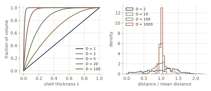
Note. The curse is real but not fatal, which is why machine learning works at all. Real data usually lie near a much lower-dimensional set inside the input space (images of handwritten digits vary in only a few ways: stroke thickness, slant, position), and real functions are usually smooth, so that nearby inputs give similar outputs and we can interpolate. The models in this course exploit one or both properties.
Decision theory
Probability theory tells us how uncertain we are. Decision theory tells us what to do about it. We split every problem into two stages: the inference stage, where the training data are turned into a model of \(p(\mathbf{x}, t)\) or of the part we need, and the decision stage, in which we use those probabilities to choose an action. Given the probabilities, the decision stage is usually easy, as we now show.
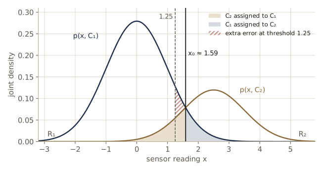
Our running example: a vibration sensor on a machine bearing gives a reading \(x\). The bearing is either normal (class \(\mathcal{C}_1\)) or worn (class \(\mathcal{C}_2\)), with prior probabilities \(p(\mathcal{C}_1) = 0.7\) and \(p(\mathcal{C}_2) = 0.3\). The class-conditional densities are Gaussian with means 0 and 2.5 and common variance 1. By Bayes’ theorem, the posterior class probabilities are
\[p(\mathcal{C}_k \mid x) = \frac{p(x \mid \mathcal{C}_k)\, p(\mathcal{C}_k)}{\sum_j p(x \mid \mathcal{C}_j)\, p(\mathcal{C}_j)}.\]priors = np.array([0.7, 0.3])
means, var_c = np.array([0.0, 2.5]), 1.0
xg = np.linspace(-6, 9, 150_001) # grid for numerical integrals
def joint(x):
"""p(x, C_k) = p(x | C_k) p(C_k), shape (len(x), 2)."""
return np.stack([gauss_pdf(x, means[k], var_c) * priors[k] for k in range(2)], axis=1)
def class_posterior(x):
j = joint(np.atleast_1d(x))
return j / j.sum(axis=1, keepdims=True)
print("x p(C1|x) p(C2|x)")
for xv in [0.0, 1.0, 1.5, 2.0, 3.0]:
post = class_posterior(xv)[0]
print(f"{xv:4.1f} {post[0]:.4f} {post[1]:.4f}")
x      p(C1|x)  p(C2|x)
 0.0   0.9815   0.0185
 1.0   0.8134   0.1866
 1.5   0.5553   0.4447
 2.0   0.2635   0.7365
 3.0   0.0285   0.9715
Minimizing the misclassification rate
A classification rule divides the input space into decision regions \(\mathcal{R}_k\): every \(x\) in \(\mathcal{R}_k\) is assigned to \(\mathcal{C}_k\). The boundaries between them are decision boundaries. A region need not be connected. With two classes, we make a mistake when a \(\mathcal{C}_1\) point falls in \(\mathcal{R}_2\) or vice versa:
\[p(\text{mistake}) = \int_{\mathcal{R}_1} p(x, \mathcal{C}_2)\, dx + \int_{\mathcal{R}_2} p(x, \mathcal{C}_1)\, dx .\]We are free to put each \(x\) in either region. To make the sum as small as possible, put \(x\) in the region whose class has the larger joint density \(p(x, \mathcal{C}_k)\), so that the smaller one is the one counted as error. Since \(p(x, \mathcal{C}_k) = p(\mathcal{C}_k \mid x) p(x)\) and \(p(x)\) is common to both classes, the misclassification rate is minimized by assigning each \(x\) to the class with the largest posterior probability \(p(\mathcal{C}_k \mid x)\). The same holds for \(K\) classes.
For our two Gaussians with equal variance, the posteriors cross where \(p(\mathcal{C}_1)\mathcal{N}(x \mid \mu_1, \sigma^2) = p(\mathcal{C}_2)\mathcal{N}(x \mid \mu_2, \sigma^2)\); taking logs, the quadratic terms cancel and the threshold is
\[x_0 = \frac{\mu_1 + \mu_2}{2} + \frac{\sigma^2}{\mu_2 - \mu_1} \ln \frac{p(\mathcal{C}_1)}{p(\mathcal{C}_2)} .\]The more common class gets the benefit of the doubt: the threshold moves toward the rarer class’s mean.
def error_rate(threshold):
    """p(mistake) for the rule: C2 if x > threshold, else C1."""
    j = joint(xg)
    in_R1 = xg <= threshold
    return (np.trapezoid(np.where(in_R1, j[:, 1], 0), xg)       # C2 points in R1
            + np.trapezoid(np.where(in_R1, 0, j[:, 0]), xg))   # C1 points in R2

x0 = means.mean() + var_c / (means[1] - means[0]) * np.log(priors[0] / priors[1])
thresholds = np.linspace(-1, 4, 5001)
errs = [error_rate(th) for th in thresholds[::10]]
print(f"threshold from the formula x0 = {x0:.4f}   "
      f"best on a grid = {thresholds[::10][np.argmin(errs)]:.3f}")
for th in [x0, 1.25, 2.0]:
    print(f"threshold {th:.3f}:  p(mistake) = {error_rate(th):.4f}")
threshold from the formula x0 = 1.5889   best on a grid = 1.590
threshold 1.589:  p(mistake) = 0.0936
threshold 1.250:  p(mistake) = 0.1056
threshold 2.000:  p(mistake) = 0.1085
Minimizing the expected loss
Not all mistakes cost the same. Missing a worn bearing may lead to a breakdown; inspecting a healthy one costs a technician’s hour. We express this with a loss matrix \(L\) whose entry \(L_{kj}\) is the cost of choosing class \(j\) when the truth is class \(k\). The average loss over inputs and true classes is
\[\mathbb{E}[L] = \sum_k \sum_j \int_{\mathcal{R}_j} L_{kj}\, p(\mathbf{x}, \mathcal{C}_k)\, d\mathbf{x}.\]As before, each \(\mathbf{x}\) can be placed independently, so we assign it to the \(j\) that minimizes \(\sum_k L_{kj}\, p(\mathcal{C}_k \mid \mathbf{x})\): the decision with the smallest expected cost given what we know about \(\mathbf{x}\). (With \(L_{kj} = 1 - \delta_{kj}\), which charges 1 for every error, this is again the largest-posterior rule.) Take \(L = \begin{pmatrix} 0 & 1 \\ 20 & 0 \end{pmatrix}\): missing a worn bearing costs 20 times as much as an unnecessary inspection. The rule becomes “declare worn when \(20\, p(\mathcal{C}_2 \mid x) > p(\mathcal{C}_1 \mid x)\)”, which moves the threshold left.
Lmat = np.array([[0.0, 1.0],       # truth C1: deciding C1 costs 0, deciding C2 costs 1
                 [20.0, 0.0]])     # truth C2: deciding C1 costs 20, deciding C2 costs 0

def expected_loss(threshold):
    j = joint(xg)
    decide = (xg > threshold).astype(int)          # 0 = C1, 1 = C2
    return sum(np.trapezoid(Lmat[k, decide] * j[:, k], xg) for k in range(2))

risk = class_posterior(xg) @ Lmat          # column j: expected loss of deciding C_j
x0_loss = xg[np.argmax(risk[:, 1] < risk[:, 0])]   # first x where deciding C2 is cheaper
x0_formula = means.mean() + np.log(priors[0] / (20 * priors[1])) / 2.5
print(f"loss-minimizing threshold {x0_loss:.3f}  (formula {x0_formula:.3f})")
for th in [x0, x0_loss]:
    print(f"threshold {th:.3f}:  expected loss {expected_loss(th):.4f}   "
          f"p(mistake) {error_rate(th):.4f}")
loss-minimizing threshold 0.391  (formula 0.391)
threshold 1.589:  expected loss 1.1260   p(mistake) 0.0936
threshold 0.391:  expected loss 0.3484   p(mistake) 0.2488
The loss-minimizing rule makes more mistakes than the error-minimizing one, but they are the cheap kind, and its expected loss is less than a third as large. The formula in the code is the threshold formula with \(p(\mathcal{C}_1)\) replaced by \(L_{12}\,p(\mathcal{C}_1)\) and \(p(\mathcal{C}_2)\) by \(L_{21}\,p(\mathcal{C}_2)\).
The reject option
Mistakes concentrate where the largest posterior is not much bigger than the others. In some applications it is better to refuse to decide there and pass the case to a human. The reject option does this: reject \(\mathbf{x}\) when \(\max_k p(\mathcal{C}_k \mid \mathbf{x}) < \theta\) for a threshold \(\theta\). With \(K\) classes, \(\theta = 1/K\) rejects nothing and \(\theta = 1\) rejects everything. (Rejection can also be built into the loss matrix, with a fixed cost for rejecting; Bishop exercise 1.24.)
post_g = class_posterior(xg)
p_x = joint(xg).sum(axis=1)
print("theta   rejected   error rate among accepted")
for theta in [0.5, 0.8, 0.9, 0.95, 0.99]:
    accept = post_g.max(axis=1) >= theta
    rej = np.trapezoid(np.where(accept, 0, p_x), xg)
    err = np.trapezoid(np.where(accept, (1 - post_g.max(axis=1)) * p_x, 0), xg)
    print(f"{theta:5.2f}   {rej:8.3f}   {err / (1 - rej):.4f}")
theta   rejected   error rate among accepted
 0.50      0.000   0.0936
 0.80      0.181   0.0399
 0.90      0.298   0.0225
 0.95      0.412   0.0127
 0.99      0.665   0.0033
Rejecting the least clear 18% of readings more than halves the error rate on the rest; rejecting 30% cuts it to about a quarter of its original value.
Inference and decision
There are three broad ways to solve a classification problem, in decreasing order of what they model:
- Generative models. Learn the class-conditional densities \(p(\mathbf{x} \mid \mathcal{C}_k)\) and the priors \(p(\mathcal{C}_k)\) (or the joint \(p(\mathbf{x}, \mathcal{C}_k)\) directly), then get the posteriors with Bayes’ theorem. They are called generative because we could sample from the model to generate synthetic inputs.
- Discriminative models. Learn the posteriors \(p(\mathcal{C}_k \mid \mathbf{x})\) directly, then decide.
- Discriminant functions. Learn a function \(f(\mathbf{x})\) that maps each input straight to a class label. Probabilities play no role.
The generative approach asks the most of the data: for high-dimensional \(\mathbf{x}\), learning \(p(\mathbf{x} \mid \mathcal{C}_k)\) accurately may need a large training set, and much of the structure in those densities may not affect the posteriors at all. In return it also gives \(p(\mathbf{x})\), which can flag inputs that the model has rarely seen (outlier or novelty detection). Here is the generative recipe on 200 labeled readings from our bearing example, with Gaussian class-conditional densities fitted by maximum likelihood:
gen = np.random.default_rng(6)
labels = (gen.random(200) < priors[1]).astype(int)            # 0 = normal, 1 = worn
readings = gen.normal(means[labels], np.sqrt(var_c))
pri_hat = np.bincount(labels, minlength=2) / 200
mu_hat = np.array([readings[labels == k].mean() for k in range(2)])
var_hat = np.mean((readings - mu_hat[labels]) ** 2)     # shared variance (ML)
x0_hat = (mu_hat.mean()
          + var_hat / (mu_hat[1] - mu_hat[0]) * np.log(pri_hat[0] / pri_hat[1]))
print(f"estimated priors {pri_hat}, means {mu_hat}, variance {var_hat:.3f}")
print(f"learned threshold {x0_hat:.3f} (optimal {x0:.3f})")
print(f"true p(mistake): learned {error_rate(x0_hat):.4f}   optimal {error_rate(x0):.4f}")
estimated priors [0.71 0.29], means [-0.0799  2.5881], variance 1.044
learned threshold 1.604 (optimal 1.589)
true p(mistake): learned 0.0936   optimal 0.0936
With 200 examples, the learned threshold is within 0.02 of the optimal one, and its error rate agrees with the optimum to four digits.
The discriminative approach needs less: in module 04 we fit \(p(\mathcal{C}_k \mid \mathbf{x})\) directly with logistic regression. A discriminant function asks least of all: it would just learn the threshold. But then we lose the posterior probabilities, which are valuable for several reasons:
- Changing losses. If the loss matrix changes, a model of the posteriors lets us recompute the decision rule at once; a discriminant function must be retrained.
- Rejection. The reject option needs posteriors.
- Compensating for class priors. When one class is rare, we often train on a balanced data set. The posteriors from that data set can be corrected afterward: divide by the class fractions in the training set, multiply by the fractions in the population, and renormalize. This works because, by Bayes’ theorem, the posterior is proportional to the prior.
- Combining models. If two sources of evidence, say \(\mathbf{x}_A\) and \(\mathbf{x}_B\), are independent given the class, \(p(\mathbf{x}_A, \mathbf{x}_B \mid \mathcal{C}_k) = p(\mathbf{x}_A \mid \mathcal{C}_k)\, p(\mathbf{x}_B \mid \mathcal{C}_k)\), then separately trained models can be combined as \(p(\mathcal{C}_k \mid \mathbf{x}_A, \mathbf{x}_B) \propto p(\mathcal{C}_k \mid \mathbf{x}_A)\, p(\mathcal{C}_k \mid \mathbf{x}_B) / p(\mathcal{C}_k)\). This conditional independence assumption is the naive Bayes model; module 08 treats conditional independence in general.
The prior correction takes three lines. Suppose a model was trained where the two classes were equally common, so it learned the balanced posteriors; we convert them to our population with priors 0.7 and 0.3.
def posterior_with_priors(x, pri):
    j = np.stack([gauss_pdf(x, means[k], var_c) * pri[k] for k in range(2)], axis=1)
    return j / j.sum(axis=1, keepdims=True)

xs5 = np.array([0.0, 1.0, 1.5, 2.0, 3.0])
balanced = posterior_with_priors(xs5, np.array([0.5, 0.5]))   # the balanced model
corrected = balanced / 0.5 * priors      # divide by training fractions, times population
corrected /= corrected.sum(axis=1, keepdims=True)                # renormalize
print("balanced p(C2|x): ", balanced[:, 1])
print("corrected p(C2|x):", corrected[:, 1])
print("true p(C2|x):     ", class_posterior(xs5)[:, 1])
balanced p(C2|x):  [0.0421 0.3486 0.6514 0.867  0.9876]
corrected p(C2|x): [0.0185 0.1866 0.4447 0.7365 0.9715]
true p(C2|x):      [0.0185 0.1866 0.4447 0.7365 0.9715]
The corrected posteriors match the true ones exactly, without retraining anything.
Loss functions for regression
For regression the decision is a number: for each \(\mathbf{x}\) we choose an estimate \(y(\mathbf{x})\) of \(t\) and pay a loss \(L(t, y(\mathbf{x}))\). With the squared loss \(L = \{y(\mathbf{x}) - t\}^2\), the expected loss is
\[\mathbb{E}[L] = \iint \{ y(\mathbf{x}) - t \}^2 p(\mathbf{x}, t)\, d\mathbf{x}\, dt .\]We want the function \(y(\mathbf{x})\) that minimizes it. Since \(y(\mathbf{x})\) can be chosen separately at each \(\mathbf{x}\), we minimize \(\int \{y - t\}^2 p(t \mid \mathbf{x})\, dt\) for each \(\mathbf{x}\); setting its derivative with respect to \(y\) to zero gives \(2\int (y - t)\, p(t \mid \mathbf{x})\, dt = 0\). (Formally this is a derivative with respect to a function, a functional derivative; Bishop’s Appendix D covers the calculus of variations.) So under squared loss the optimal prediction is the conditional mean, called the regression function:
\[y(\mathbf{x}) = \mathbb{E}[t \mid \mathbf{x}] = \int t\, p(t \mid \mathbf{x})\, dt .\]Adding and subtracting \(\mathbb{E}[t \mid \mathbf{x}]\) inside the square, the cross term integrates to zero over \(t\), and we get
\[\mathbb{E}[L] = \int \bigl\{ y(\mathbf{x}) - \mathbb{E}[t \mid \mathbf{x}] \bigr\}^2 p(\mathbf{x})\, d\mathbf{x} + \int \operatorname{var}[t \mid \mathbf{x}]\, p(\mathbf{x})\, d\mathbf{x}.\]The first term depends on our choice of \(y\) and vanishes at the regression function. The second is the intrinsic noise in the targets, which no predictor can remove. For our sine data the regression function is \(\sin(2\pi x)\) and the noise variance is \(0.3^2 = 0.09\), so the expected squared loss of any fitted curve should be its mean squared distance from the sine plus 0.09. With the large test set:
for M in [3, 9]:
    w = fit_poly(x, t, M)
    mse = np.mean((predict(w, x_test) - t_test) ** 2)
    gap = np.mean((predict(w, x_test) - np.sin(2 * np.pi * x_test)) ** 2)
    print(f"M = {M}:  test mean squared loss {mse:.4f}   "
          f"= distance to sin {gap:.4f} + noise {mse - gap:.4f}")
M = 3:  test mean squared loss 0.1026   = distance to sin 0.0132 + noise 0.0895
M = 9:  test mean squared loss 0.5820   = distance to sin 0.4927 + noise 0.0894
The “noise” part comes out close to 0.09 in both cases, as it should, and all the difference between the models is in the first term.
As with classification, we can model the joint density, or model \(p(t \mid \mathbf{x})\) and then take its mean, or fit a function \(y(\mathbf{x})\) to the data directly. And other losses call for other summaries of \(p(t \mid \mathbf{x})\). The Minkowski loss \(L_q = \lvert y - t \rvert^q\) reduces to squared loss at \(q = 2\). Its minimizer is the conditional median at \(q = 1\), and as \(q\) shrinks toward 0 it moves toward the conditional mode. Let us check on a conditional density with two bumps, a narrow one at 1 and a broad one at 3, so that the mean, the median, and the mode are all different.
tg = np.linspace(-4, 10, 14_001)
p_t = 0.4 * gauss_pdf(tg, 1.0, 0.3 ** 2) + 0.6 * gauss_pdf(tg, 3.0, 1.0)   # p(t | x), fixed x
cdf = np.cumsum(p_t) * (tg[1] - tg[0])
print(f"mean {np.trapezoid(tg * p_t, tg):.3f}   median {tg[np.searchsorted(cdf, 0.5)]:.3f}   "
      f"mode {tg[np.argmax(p_t)]:.3f}")
y_cand = np.linspace(0, 4, 801)
for q in [2, 1, 0.5, 0.1]:
    expected = [np.trapezoid(np.abs(yc - tg) ** q * p_t, tg) for yc in y_cand]
    print(f"q = {q:>3}:  minimizer of E[|y - t|^q] = {y_cand[np.argmin(expected)]:.3f}")
eps = 0.05                                      # 0-1 loss: pay 1 unless |y - t| < eps
hit = [np.trapezoid(p_t * (np.abs(yc - tg) < eps), tg) for yc in y_cand]
print(f"0-1 loss with eps = {eps}: minimizer = {y_cand[np.argmax(hit)]:.3f}")
mean 2.200   median 2.033   mode 1.011
q =   2:  minimizer of E[|y - t|^q] = 2.200
q =   1:  minimizer of E[|y - t|^q] = 2.035
q = 0.5:  minimizer of E[|y - t|^q] = 1.275
q = 0.1:  minimizer of E[|y - t|^q] = 1.120
0-1 loss with eps = 0.05: minimizer = 1.000
Watch out. At \(q = 2\) and \(q = 1\) the minimizers match the mean and the median exactly. For small \(q\) the minimizer approaches the mode but, strictly, the limit \(q \to 0\) minimizes the average of \(\ln\lvert y - t \rvert\), which is not quite the mode. The loss whose minimizer is the mode is the 0–1 loss “pay 1 unless you are within \(\epsilon\) of \(t\)”, as \(\epsilon \to 0\) (last line of the output).
Information theory
The last tool of the chapter measures information. It will give us a way to compare distributions (the KL divergence), which appears throughout the course, from maximum likelihood to the variational methods of module 10.
Entropy
How much information do we receive when we observe a discrete random variable \(x\) take a value? A rare value tells us more than a common one; for two independent observations the information should add, \(h(x, y) = h(x) + h(y)\), while their probabilities multiply. A logarithm has exactly these properties, so we define the information content of an outcome as
\[h(x) = -\log_2 p(x),\]measured in bits. Its average over the distribution is the entropy,
\[\mathrm{H}[x] = -\sum_x p(x) \log_2 p(x),\]with the convention \(0 \log 0 = 0\) (the limit of \(p \ln p\) as \(p \to 0\)). An example: tomorrow’s weather is sunny, cloudy, rainy, or snowy with probabilities \(\tfrac12, \tfrac14, \tfrac18, \tfrac18\). The entropy is \(\tfrac12 \cdot 1 + \tfrac14 \cdot 2 + 2 \cdot \tfrac18 \cdot 3 = 1.75\) bits. If we want to send the forecast as a string of bits, two bits per message suffice (four outcomes), but we can do better on average by using short codewords for common outcomes: 0 for sunny, 10 for cloudy, 110 for rainy, 111 for snowy. No codeword is the start of another (a prefix code), so a string of them can be decoded without separators.
def entropy(p, base=np.e):
    """H[p] = -sum p ln p, with 0 ln 0 = 0; in nats by default, bits with base=2."""
    p = np.asarray(p, dtype=float)
    nz = p > 0
    return -np.sum(p[nz] * np.log(p[nz])) / np.log(base)

weather = np.array([1/2, 1/4, 1/8, 1/8])
code = ["0", "10", "110", "111"]
avg_len = sum(pw * len(c) for pw, c in zip(weather, code))
print(f"entropy {entropy(weather, 2):.3f} bits   average code length {avg_len:.3f} bits")
print(f"entropy of the uniform distribution on 4 states: {entropy(np.full(4, 0.25), 2):.3f} bits")

msgs = np.random.default_rng(7).choice(4, size=100_000, p=weather)
bits = sum(len(code[m]) for m in msgs)
print(f"100,000 simulated forecasts: {bits / len(msgs):.4f} bits per forecast")
entropy 1.750 bits   average code length 1.750 bits
entropy of the uniform distribution on 4 states: 2.000 bits
100,000 simulated forecasts: 1.7523 bits per forecast
The average code length equals the entropy here, and that is no accident: Shannon’s noiseless coding theorem says that no code can use fewer bits per message, on average, than the entropy of the source, and codes like this one can come close to it. With natural logarithms, entropy is measured in nats; one nat is \(1/\ln 2 \approx 1.44\) bits. From now on we use natural logs.
Entropy as counting. Entropy also has a physical reading. Put \(N\) distinguishable objects into bins so that bin \(i\) gets \(n_i\) of them. The number of ways to do this, ignoring the order within each bin, is the multiplicity \(W = N! / \prod_i n_i!\). Using Stirling’s approximation \(\ln N! \approx N \ln N - N\) and letting \(N \to \infty\) with fractions \(p_i = n_i/N\) held fixed, \(\frac{1}{N} \ln W \to -\sum_i p_i \ln p_i\). A spread-out distribution can be realized in many more ways than a peaked one.
for N in [16, 160, 16_000, 1_600_000]:
    n_i = (weather * N).astype(int)
    lnW = gammaln(N + 1) - gammaln(n_i + 1).sum()
    print(f"N = {N:>9}:  (1/N) ln W = {lnW / N:.5f}   H = {entropy(weather):.5f} nats")
N =        16:  (1/N) ln W = 0.96893   H = 1.21301 nats
N =       160:  (1/N) ln W = 1.16762   H = 1.21301 nats
N =     16000:  (1/N) ln W = 1.21212   H = 1.21301 nats
N =   1600000:  (1/N) ln W = 1.21299   H = 1.21301 nats
Maximum entropy. Over distributions on \(M\) states, the entropy is largest for the uniform distribution. To show it, maximize \(-\sum_i p_i \ln p_i\) subject to \(\sum_i p_i = 1\) with a Lagrange multiplier \(\lambda\) (Bishop Appendix E): the stationarity condition \(-\ln p_i - 1 + \lambda = 0\) makes every \(p_i\) the same, so \(p_i = 1/M\) and \(\mathrm{H} = \ln M\). The second derivative, \(-1/p_i\) on the diagonal, shows it is a maximum. The minimum, \(\mathrm{H} = 0\), is reached when one state has probability 1. A check with random distributions:
dirichlet = np.random.default_rng(8).dirichlet(np.ones(6), size=100_000)   # rows: distributions
H = -np.sum(dirichlet * np.log(dirichlet), axis=1)
print(f"largest entropy of 100,000 random distributions: {H.max():.4f}   ln 6 = {np.log(6):.4f}")
largest entropy of 100,000 random distributions: 1.7880 ln 6 = 1.7918
Differential entropy
For a continuous variable, divide the real line into bins of width \(\Delta\). The discrete entropy of the binned variable is approximately \(-\int p(x) \ln p(x)\, dx - \ln \Delta\), and the second term diverges as \(\Delta \to 0\): specifying a real number exactly takes infinitely many bits. Dropping it defines the differential entropy
\[\mathrm{H}[x] = -\int p(x) \ln p(x)\, dx .\]Which density has the largest differential entropy? Without constraints the question has no answer, but with the mean and variance fixed it does. Maximizing \(-\int p \ln p\, dx\) subject to normalization, a given mean \(\mu\), and a given variance \(\sigma^2\), with three Lagrange multipliers and the calculus of variations, forces \(\ln p(x)\) to be a quadratic in \(x\), so \(p\) must be a Gaussian (Bishop §1.6 has the details). For a fixed variance \(\sigma^2\), then, the Gaussian has the largest differential entropy, which works out to
\[\mathrm{H}[x] = \tfrac12 \bigl\{ 1 + \ln(2\pi\sigma^2) \bigr\}.\]Unlike discrete entropy, differential entropy can be negative: it is below zero whenever \(\sigma^2 < 1/(2\pi e)\). Let us check the binning relation and compare the Gaussian with a Laplace and a uniform density of the same variance.
sig = 0.8
H_gauss = 0.5 * (1 + np.log(2 * np.pi * sig ** 2))
xq = np.linspace(-12, 12, 480_001)
pg = gauss_pdf(xq, 0.0, sig ** 2)
H_num = -np.trapezoid(pg * np.log(pg + 1e-300), xq)
print(f"Gaussian: formula {H_gauss:.5f}   numerical {H_num:.5f}")

for Delta in [0.5, 0.1, 0.01]:
    edges = np.arange(-12, 12 + Delta, Delta)
    probs = np.diff(0.5 * (1 + erf(edges / (sig * np.sqrt(2)))))   # bin probabilities
    print(f"Delta = {Delta:4}:  H[binned] + ln Delta = {entropy(probs) + np.log(Delta):.5f}")

b = sig / np.sqrt(2)                   # Laplace with variance 2 b^2 = sig^2
width = sig * np.sqrt(12)              # uniform with variance width^2 / 12 = sig^2
print(f"same variance:  Gaussian {H_gauss:.4f}   Laplace {1 + np.log(2 * b):.4f}   "
      f"uniform {np.log(width):.4f}")
print(f"a narrow Gaussian (sigma = 0.1): H = {0.5 * (1 + np.log(2 * np.pi * 0.01)):.4f} nats")
Gaussian: formula 1.19579   numerical 1.19579
Delta =  0.5:  H[binned] + ln Delta = 1.21181
Delta =  0.1:  H[binned] + ln Delta = 1.19645
Delta = 0.01:  H[binned] + ln Delta = 1.19580
same variance:  Gaussian 1.1958   Laplace 1.1234   uniform 1.0193
a narrow Gaussian (sigma = 0.1): H = -0.8836 nats
Conditional entropy. For a joint distribution \(p(\mathbf{x}, \mathbf{y})\), the average additional information needed to specify \(\mathbf{y}\) once \(\mathbf{x}\) is known is the conditional entropy
\[\mathrm{H}[\mathbf{y} \mid \mathbf{x}] = -\iint p(\mathbf{y}, \mathbf{x}) \ln p(\mathbf{y} \mid \mathbf{x})\, d\mathbf{y}\, d\mathbf{x}.\]Taking logs of the product rule gives the chain rule \(\mathrm{H}[\mathbf{x}, \mathbf{y}] = \mathrm{H}[\mathbf{y} \mid \mathbf{x}] + \mathrm{H}[\mathbf{x}]\): the information to describe both is the information to describe \(\mathbf{x}\) plus the extra for \(\mathbf{y}\) given \(\mathbf{x}\). With the joint table from the probability section:
H_joint = entropy(P_XY.ravel())
H_X = entropy(p_X)
H_Y_given_X = -np.sum(P_XY * np.log(p_Y_given_X))
print(f"H[X,Y] = {H_joint:.4f}   "
      f"H[Y|X] + H[X] = {H_Y_given_X:.4f} + {H_X:.4f} = {H_Y_given_X + H_X:.4f}")
print(f"H[Y] = {entropy(P_XY.sum(axis=0)):.4f}  (knowing X lowers it to {H_Y_given_X:.4f})")
H[X,Y] = 1.6796   H[Y|X] + H[X] = 0.5836 + 1.0961 = 1.6796
H[Y] = 0.6474  (knowing X lowers it to 0.5836)
Relative entropy and mutual information
Suppose data come from a distribution \(p(\mathbf{x})\) but we build our code, or our model, from a different distribution \(q(\mathbf{x})\). The average extra information this costs is the relative entropy or Kullback–Leibler (KL) divergence
\[\mathrm{KL}(p \Vert q) = -\int p(\mathbf{x}) \ln q(\mathbf{x})\, d\mathbf{x} - \Bigl( -\int p(\mathbf{x}) \ln p(\mathbf{x})\, d\mathbf{x} \Bigr) = -\int p(\mathbf{x}) \ln \frac{q(\mathbf{x})}{p(\mathbf{x})}\, d\mathbf{x}\](with a sum for discrete variables). It is not symmetric: in general \(\mathrm{KL}(p \Vert q) \ne \mathrm{KL}(q \Vert p)\). Its key property is that it is never negative. To prove it we need convexity.
A function \(f\) is convex if every chord lies on or above the graph: \(f(\lambda a + (1 - \lambda) b) \le \lambda f(a) + (1 - \lambda) f(b)\) for all \(a, b\) and \(0 \le \lambda \le 1\). It is strictly convex if equality holds only at \(\lambda = 0\) and \(\lambda = 1\) (for \(a \ne b\)). A twice-differentiable function with \(f'' > 0\) everywhere is strictly convex; \(x^2\), \(e^x\), and \(-\ln x\) (for \(x > 0\)) are examples. If \(f\) is convex, \(-f\) is concave.
By induction on the number of points, convexity extends to any weighted average with weights \(\lambda_i \ge 0\) summing to one, \(f\bigl(\sum_i \lambda_i x_i\bigr) \le \sum_i \lambda_i f(x_i)\). Reading the weights as probabilities gives Jensen’s inequality:
\[f\bigl(\mathbb{E}[x]\bigr) \le \mathbb{E}\bigl[f(x)\bigr] \quad\text{for convex } f, \qquad\text{and more generally}\qquad f\bigl(\mathbb{E}[\xi(x)]\bigr) \le \mathbb{E}\bigl[f(\xi(x))\bigr].\]Apply it with the convex function \(f = -\ln\) and \(\xi(\mathbf{x}) = q(\mathbf{x}) / p(\mathbf{x})\), averaging under \(p\):
\[\mathrm{KL}(p \Vert q) = \mathbb{E}_p\left[ -\ln \frac{q(\mathbf{x})}{p(\mathbf{x})} \right] \ge -\ln \mathbb{E}_p\left[ \frac{q(\mathbf{x})}{p(\mathbf{x})} \right] = -\ln \int q(\mathbf{x})\, d\mathbf{x} = -\ln 1 = 0.\]Because \(-\ln\) is strictly convex, equality holds only when \(q(\mathbf{x})/p(\mathbf{x})\) is constant, that is, when \(q = p\). So \(\mathrm{KL}(p \Vert q) \ge 0\), with equality if and only if the two distributions are equal, and we can read the KL divergence as a measure of how different \(q\) is from \(p\). Checks on random discrete distributions, and on two Gaussians, where the closed form is \(\mathrm{KL}(\mathcal{N}(\mu_1, \sigma_1^2) \Vert \mathcal{N}(\mu_2, \sigma_2^2)) = \ln\frac{\sigma_2}{\sigma_1} + \frac{\sigma_1^2 + (\mu_1 - \mu_2)^2}{2\sigma_2^2} - \frac12\):
def kl_discrete(p, q):
    """KL(p || q) = sum p ln(p / q), with 0 ln 0 = 0."""
    nz = p > 0
    return np.sum(p[nz] * np.log(p[nz] / q[nz]))

kr = np.random.default_rng(9)
P = kr.dirichlet(np.ones(5), size=20_000)
Q = kr.dirichlet(np.ones(5), size=20_000)
kls = np.array([kl_discrete(a, c) for a, c in zip(P, Q)])
print(f"smallest KL over 20,000 random pairs: {kls.min():.2e}   "
      f"KL(p||p) = {kl_discrete(P[0], P[0]):.1f}")
print(f"asymmetry: KL(p||q) = {kl_discrete(P[0], Q[0]):.4f}   "
      f"KL(q||p) = {kl_discrete(Q[0], P[0]):.4f}")

def kl_gauss(m1, s1, m2, s2):
    return np.log(s2 / s1) + (s1 ** 2 + (m1 - m2) ** 2) / (2 * s2 ** 2) - 0.5

xs_p = kr.normal(0.0, 1.0, 1_000_000)                         # samples from p = N(0, 1)
mc = np.mean(np.log(gauss_pdf(xs_p, 0.0, 1.0)) - np.log(gauss_pdf(xs_p, 1.0, 1.5 ** 2)))
print(f"KL(N(0,1) || N(1,1.5^2)): closed form {kl_gauss(0, 1, 1, 1.5):.4f}   "
      f"Monte Carlo {mc:.4f}")
smallest KL over 20,000 random pairs: 3.63e-03   KL(p||p) = 0.0
asymmetry: KL(p||q) = 0.2775   KL(q||p) = 0.2454
KL(N(0,1) || N(1,1.5^2)): closed form 0.3499   Monte Carlo 0.3503
KL divergence and maximum likelihood. Suppose data \(\mathbf{x}_1, \dots, \mathbf{x}_N\) come from an unknown \(p(\mathbf{x})\) and we model it with a family \(q(\mathbf{x} \mid \boldsymbol{\theta})\). We would like the \(\boldsymbol{\theta}\) that minimizes \(\mathrm{KL}(p \Vert q)\), but we cannot compute it without \(p\). Replacing the expectation under \(p\) by an average over the data,
\[\mathrm{KL}(p \Vert q) \approx \frac{1}{N} \sum_{n=1}^{N} \bigl\{ -\ln q(\mathbf{x}_n \mid \boldsymbol{\theta}) + \ln p(\mathbf{x}_n) \bigr\}.\]The second term does not depend on \(\boldsymbol{\theta}\), and the first is the negative log-likelihood divided by \(N\). So maximizing the likelihood is minimizing an estimate of \(\mathrm{KL}(p \Vert q)\), the divergence between the data distribution and the model. This is one reason the KL divergence shows up so often in machine learning.
Mutual information. Two variables are independent when \(p(\mathbf{x}, \mathbf{y}) = p(\mathbf{x})p(\mathbf{y})\). The KL divergence from the joint to the product of the marginals measures how far they are from independent; it is the mutual information
\[\mathrm{I}[\mathbf{x}, \mathbf{y}] = \mathrm{KL}\bigl( p(\mathbf{x}, \mathbf{y}) \Vert p(\mathbf{x}) p(\mathbf{y}) \bigr) = -\iint p(\mathbf{x}, \mathbf{y}) \ln \frac{p(\mathbf{x}) p(\mathbf{y})}{p(\mathbf{x}, \mathbf{y})}\, d\mathbf{x}\, d\mathbf{y}.\]It is at least zero, with equality exactly for independent variables. Using the sum and product rules it can be rewritten as \(\mathrm{I}[\mathbf{x}, \mathbf{y}] = \mathrm{H}[\mathbf{x}] - \mathrm{H}[\mathbf{x} \mid \mathbf{y}] = \mathrm{H}[\mathbf{y}] - \mathrm{H}[\mathbf{y} \mid \mathbf{x}]\): the reduction in our uncertainty about one variable from learning the other. In Bayesian terms, if \(\mathbf{x}\) is a parameter and \(\mathbf{y}\) the data, it is the average amount by which the data shrink the uncertainty from prior to posterior.
p_Y = P_XY.sum(axis=0)
I_kl = kl_discrete(P_XY.ravel(), np.outer(p_X, p_Y).ravel())
I_ent = entropy(p_Y) - H_Y_given_X
print(f"I[X,Y] as a KL divergence: {I_kl:.4f} nats   as H[Y] - H[Y|X]: {I_ent:.4f} nats")
indep = np.outer(p_X, p_Y)          # the independent joint with the same marginals
print(f"for the independent joint: I = {kl_discrete(indep.ravel(), indep.ravel()):.4f}")
I[X,Y] as a KL divergence: 0.0639 nats   as H[Y] - H[Y|X]: 0.0639 nats
for the independent joint: I = 0.0000
Summary
| Idea | What it says | Where it returns |
|---|---|---|
| Least squares | minimize \(\tfrac12\sum_n (y(x_n, \mathbf{w}) - t_n)^2\); solve \(\mathbf{\Phi}^{\mathrm{T}}\mathbf{\Phi}\mathbf{w} = \mathbf{\Phi}^{\mathrm{T}}\mathbf{t}\) | module 03 |
| Regularization (ridge) | add \(\tfrac{\lambda}{2}\lVert \mathbf{w} \rVert^2\); solve \((\mathbf{\Phi}^{\mathrm{T}}\mathbf{\Phi} + \lambda\mathbf{I})\mathbf{w} = \mathbf{\Phi}^{\mathrm{T}}\mathbf{t}\) | modules 03, 05 |
| Sum and product rules, Bayes’ theorem | \(p(Y \mid X) = p(X \mid Y)p(Y)/p(X)\); posterior ∝ likelihood × prior | every module |
| Change of variables | \(p_y(y) = p_x(g(y))\,\lvert g'(y) \rvert\); modes are not invariant | modules 02, 11 |
| Gaussian maximum likelihood | sample mean; sample variance, biased by \((N-1)/N\) | module 02 |
| Least squares as ML, ridge as MAP | Gaussian noise gives squared error; a Gaussian prior gives \(\lambda = \alpha/\beta\) | module 03 |
| Model selection | validation set, S-fold cross-validation, AIC/BIC | modules 03, 04 |
| Decision theory | largest posterior minimizes errors; minimize \(\sum_k L_{kj}\,p(\mathcal{C}_k \mid \mathbf{x})\) for general losses; conditional mean for squared loss | modules 04, 05, 07 |
| Information theory | entropy; Gaussian has maximum entropy for a given variance; \(\mathrm{KL}(p \Vert q) \ge 0\); ML minimizes an estimate of KL | modules 09, 10 |
Ideas to carry forward:
- The training error is not the goal. A flexible model fitted by maximum likelihood fits the noise; regularization, more data, a prior, or model selection with held-out data are the remedies.
- Keep inference and decision separate. Learn probabilities first, then choose the action that minimizes expected loss; the probabilities let you change losses, reject doubtful cases, and correct for class priors without retraining.
- Many familiar recipes are probabilistic statements in disguise: least squares is Gaussian maximum likelihood, ridge regression is a Gaussian prior, and maximum likelihood minimizes a KL divergence.
- High-dimensional spaces are not like the plane. Methods that divide the space into cells, or rely on “nearby” points, need either huge data sets or models that exploit structure in the data.
Exercises
- Show that the regularized error \(\widetilde{E}(\mathbf{w})\) is minimized by the solution of \((\mathbf{\Phi}^{\mathrm{T}}\mathbf{\Phi} + \lambda\mathbf{I})\mathbf{w} = \mathbf{\Phi}^{\mathrm{T}}\mathbf{t}\), and prove that this matrix is invertible for every \(\lambda > 0\), whatever \(N\) and \(M\) are. (Hint: show that \(\mathbf{v}^{\mathrm{T}}(\mathbf{\Phi}^{\mathrm{T}}\mathbf{\Phi} + \lambda\mathbf{I})\mathbf{v} > 0\) for \(\mathbf{v} \ne \mathbf{0}\).)
- Modify
fit_polyso that \(w_0\) is not penalized. Show on the ten-point data that adding 5 to every target changes the fitted curve by exactly 5 with this version but not with the original. - A medical lab test for a condition with 2% prevalence has a false negative rate of 5% and a false positive rate of 3%. Compute the probability of having the condition after one positive test, and after two positive results on independent retests. Verify both by simulation, as in the spam example.
- Let \(x\) be uniform on \((0, 1)\) and \(y = -\ln x\). Find \(p_y(y)\) with the change-of-variables formula, and check it against a histogram of samples. Then do the same for \(y = x^2\), and explain why the density of \(y\) is unbounded near 0 although the density of \(x\) is not.
- Prove \(\mathbb{E}[\sigma^2_{\mathrm{ML}}] = \frac{N-1}{N}\sigma^2\) carefully, starting from \(\mathbb{E}[x_n x_m] = \mu^2 + \sigma^2\delta_{nm}\). Then extend the simulation to show how the average of \(\sigma^2_{\mathrm{ML}}\) approaches \(\sigma^2\) for \(N = 2, 5, 20, 100\).
- For the Gaussian noise model of curve fitting, derive \(1/\beta_{\mathrm{ML}}\) by differentiating the log-likelihood with respect to \(\beta\). Then run the bias simulation for curve fitting: generate 2,000 ten-point data sets, fit \(M = 3\) to each, and compare the average of \(1/\beta_{\mathrm{ML}}\) with 0.09 and with \(\frac{N - (M+1)}{N} \cdot 0.09\). Which is closer, and why might that be?
- Implement 10-fold cross-validation over the pair \((M, \ln\lambda)\) for \(M \in \{3, 6, 9\}\) and \(\ln\lambda \in \{-25, -20, \dots, 0\}\) on the 30-point data set. How many fits does it take? Does the best pair differ much, in test error, from the best \(M\) alone?
- Show that the fraction of the volume of the \(D\)-dimensional hypercube \([-1, 1]^D\) that lies inside the inscribed unit ball goes to zero as \(D \to \infty\). Estimate the fraction by Monte Carlo for \(D = 2, 5, 10, 20\), and compare with the exact value \(\pi^{D/2} / (\Gamma(D/2 + 1)\, 2^D)\) (use
gammaln). - For \(K\) classes and a loss matrix that charges 1 for each error and \(\lambda < 1\) for rejecting, show that the rule minimizing expected loss is the reject option with \(\theta = 1 - \lambda\). Verify on the bearing example that \(\lambda = 0.1\) reproduces the \(\theta = 0.9\) row of the reject table.
- Show that the absolute loss \(\lvert y - t \rvert\) is minimized by the median of \(p(t \mid \mathbf{x})\): differentiate \(\int \lvert y - t \rvert\, p(t \mid \mathbf{x})\, dt\) with respect to \(y\), splitting the integral at \(t = y\).
- Prove that the entropy of a distribution on \(M\) states satisfies \(\mathrm{H} \le \ln M\) using Jensen’s inequality instead of Lagrange multipliers. Then show that \(\mathrm{I}[x, y] = \mathrm{H}[x] + \mathrm{H}[y] - \mathrm{H}[x, y]\) and check it numerically on
P_XY. - In your own words: why does the order-9 polynomial reach zero training error but predict badly, and what do regularization, more data, and the Bayesian predictive distribution each change about that picture?
Going further
- C. M. Bishop, Pattern Recognition and Machine Learning, chapter 1 — the source for this module. Exercises 1.1–1.2 derive the normal equations with and without regularization, 1.4 is the change-of-variables mode shift, 1.11–1.12 cover Gaussian maximum likelihood and its bias, 1.18–1.20 explore spheres and Gaussians in high dimensions, 1.22–1.27 are decision-theory and loss-function exercises, and 1.29–1.41 cover entropy, KL divergence, and mutual information.
- C. E. Shannon, “A mathematical theory of communication”, Bell System Technical Journal, 1948 — the paper that founded information theory, still very readable.
- S. Kullback and R. A. Leibler, “On information and sufficiency”, Annals of Mathematical Statistics, 1951 — the origin of the KL divergence.
- T. Hastie, R. Tibshirani, and J. Friedman, The Elements of Statistical Learning, 2nd ed., Springer, 2009 (free PDF) — chapter 2 on the curse of dimensionality and chapter 7 on model assessment, cross-validation, and the bootstrap, from a frequentist angle.
- D. J. C. MacKay, Information Theory, Inference, and Learning Algorithms, Cambridge University Press, 2003 (free online) — a Bayesian’s introduction to entropy, coding, and inference, with many worked examples.
These notes follow the chapters of C. M. Bishop, Pattern Recognition and Machine Learning (Springer, 2006), the course text, which Microsoft Research makes freely available as a PDF. The explanations, code, figures, and exercises here are written for this course; the book remains the reference, with the full derivations and many more exercises.