CSE 474/574 · Module 10 · Week 11
Approximate Inference
Variational inference with factorized distributions, the variational Gaussian mixture, variational regression and logistic regression, and expectation propagation.
Companion reading: Bishop, Pattern Recognition and Machine Learning, chapter 10, “Approximate Inference”
By the end of this module you can
- Write the decomposition \(\ln p(\mathbf{X}) = \mathcal{L}(q) + \mathrm{KL}(q \Vert p)\), explain why maximizing the lower bound is the same as minimizing the KL divergence, and relate it to the EM algorithm.
- Derive the mean-field update, which sets the log of each optimal factor to the expected log joint distribution under the other factors, and use it to find the form of each factor for a new conjugate model.
- Compare the approximations that minimize \(\mathrm{KL}(q \Vert p)\) and \(\mathrm{KL}(p \Vert q)\), and predict which one underestimates variance, seeks a single mode, or spreads over all modes.
- Implement coordinate-ascent variational inference for a Gaussian with unknown mean and precision and for a Bayesian mixture of Gaussians, monitor the lower bound, and explain why unneeded mixture components switch themselves off.
- Apply variational inference to Bayesian linear regression with a gamma hyperprior, and show that it reproduces the evidence approximation of module 03.
- Use convex duality to bound a function by simpler ones, derive the Jaakkola–Jordan bound on the logistic sigmoid, and use it to fit a Gaussian posterior for logistic regression.
- Implement expectation propagation by moment matching on the clutter problem and check the posterior and the evidence against exact values computed on a grid.
- Choose between the Laplace approximation, variational Bayes, and expectation propagation for a given model, and say what each one gets wrong.
Contents
- Variational inference
- The variational mixture of Gaussians
- Variational linear regression
- Exponential family distributions
- Local variational methods
- Variational logistic regression
- Expectation propagation
- Summary
- Exercises
- Going further
Almost everything we have done with Bayesian models so far rested on one lucky fact: the posterior had a closed form. In module 02 conjugate priors made the posterior of a Gaussian mean or a Bernoulli parameter a distribution of the same family as the prior. In module 03 the posterior over regression weights was Gaussian. When the luck ran out, as with logistic regression in module 04, we replaced the posterior by a Gaussian centered at its mode, the Laplace approximation. And in module 09 we fit mixture models by EM, which needs the posterior over the latent variables but treats the parameters as fixed numbers.
Most models of practical interest are not so lucky. The posterior over the parameters of a Gaussian mixture is a sum over every way of assigning points to components, exponentially many terms. The posterior of a logistic regression has no closed form at all. We still want posterior means, predictive distributions, and the evidence for comparing models, so we need approximations. There are two broad families. Stochastic methods draw samples from the posterior and average over them; they are exact in the limit of infinite computation and are the subject of module 11. Deterministic methods replace the posterior by a simpler distribution chosen by optimization; they are never exact, but they are fast and they give closed-form answers. This module is about the deterministic family.
The main tool is variational inference: pick a family of tractable distributions and find the member closest to the posterior in the sense of a Kullback–Leibler divergence. We derive the general update for factorized families, study what kind of errors it makes, and then work four examples in NumPy: a Gaussian with unknown mean and precision, a Bayesian Gaussian mixture that decides how many components it needs, Bayesian linear regression with a prior on the prior precision, and logistic regression through a clever bound on the sigmoid. We close with expectation propagation, which minimizes the other KL divergence and often gives better answers, and we check every method against the exact posterior where we can compute it.
Variational inference
Functionals and the lower bound
A function takes a number and returns a number. A functional takes a whole function and returns a number. The entropy is an example: it takes a density \(p(x)\) and returns \(\mathrm{H}[p] = -\int p(x) \ln p(x)\, \mathrm{d}x\). Just as calculus asks how a function changes when its input moves a little, the calculus of variations asks how a functional changes when its input function is perturbed a little, and it finds the input function that maximizes or minimizes the functional. Bishop’s Appendix D has the rules; we will need only one idea from it, and we will derive what we use. “Variational” methods get their name from this: we optimize over distributions.
Here is the setting. We have observed variables \(\mathbf{X}\) and unobserved variables \(\mathbf{Z}\). In a fully Bayesian model every unknown, latent variables and parameters alike, goes into \(\mathbf{Z}\). The model gives us the joint \(p(\mathbf{X}, \mathbf{Z})\), and we want the posterior \(p(\mathbf{Z} \mid \mathbf{X})\) and the evidence \(p(\mathbf{X})\).
Take any distribution \(q(\mathbf{Z})\). By the product rule, \(\ln p(\mathbf{X}) = \ln p(\mathbf{X}, \mathbf{Z}) - \ln p(\mathbf{Z} \mid \mathbf{X})\) for every value of \(\mathbf{Z}\). Add and subtract \(\ln q(\mathbf{Z})\), multiply by \(q(\mathbf{Z})\), and integrate over \(\mathbf{Z}\). The left side does not depend on \(\mathbf{Z}\) and \(q\) integrates to one, so
\[\ln p(\mathbf{X}) = \underbrace{\int q(\mathbf{Z}) \ln \frac{p(\mathbf{X}, \mathbf{Z})}{q(\mathbf{Z})}\, \mathrm{d}\mathbf{Z}}_{\mathcal{L}(q)} \; \underbrace{- \int q(\mathbf{Z}) \ln \frac{p(\mathbf{Z} \mid \mathbf{X})}{q(\mathbf{Z})}\, \mathrm{d}\mathbf{Z}}_{\mathrm{KL}(q \Vert p)} .\]The second term is the Kullback–Leibler divergence between \(q\) and the posterior, which is never negative and is zero only when \(q\) equals the posterior. So \(\mathcal{L}(q)\) is a lower bound on the log evidence, often called the ELBO (evidence lower bound), and the gap is exactly the KL divergence. Since the left side does not depend on \(q\), raising \(\mathcal{L}(q)\) and lowering \(\mathrm{KL}(q \Vert p)\) are the same thing.
This is the decomposition that justified EM in module 09, with one change: there the parameters \(\boldsymbol{\theta}\) sat outside \(\mathbf{Z}\) as point estimates, and the E step set \(q\) equal to the exact posterior over the latent variables. Now the parameters are random too, and the exact posterior is out of reach. So we restrict \(q\) to a family of distributions we can work with and maximize \(\mathcal{L}(q)\) within that family. The restriction exists only to make the problem tractable: a richer family can only get closer to the posterior, and there is no overfitting in making \(q\) more flexible.
Note. The lower bound is useful in two ways at once. As an objective, it tells us which \(q\) to pick. As a number, it approximates \(\ln p(\mathbf{X})\), the quantity we need for comparing models, and it can never overshoot it. Every algorithm in the first half of this module increases \(\mathcal{L}(q)\) at every step, which also makes the bound a debugging tool: if it ever goes down, there is a bug.
One way to restrict \(q\) is to give it a parametric form, say a Gaussian with free mean and covariance, and maximize \(\mathcal{L}\) over those parameters with any optimizer. We will do this in effect for logistic regression. The more common restriction, which we turn to now, fixes no functional form at all and only assumes independence.
Factorized distributions
Split the unobserved variables into disjoint groups \(\mathbf{Z}_1, \dots, \mathbf{Z}_M\) and assume \(q\) factorizes over them,
\[q(\mathbf{Z}) = \prod_{i=1}^{M} q_i(\mathbf{Z}_i).\]Nothing else is assumed: each factor can have any shape. This is called mean-field variational inference, a name borrowed from physics. We maximize \(\mathcal{L}(q)\) over one factor at a time, holding the others fixed.
Write \(q_j\) for \(q_j(\mathbf{Z}_j)\) and substitute the product into the bound. The logarithm of a product is a sum, so the \(\ln q\) part splits into one entropy term per factor:
\[\mathcal{L}(q) = \int \prod_i q_i \, \ln p(\mathbf{X}, \mathbf{Z})\, \mathrm{d}\mathbf{Z} - \sum_i \int q_i \ln q_i \, \mathrm{d}\mathbf{Z}_i .\]Now look only at the dependence on \(q_j\). In the first term, integrate over all the other groups first; what remains inside the \(\mathbf{Z}_j\) integral is the expectation of the log joint under the other factors, which we write \(\mathbb{E}_{i \neq j}[\ln p(\mathbf{X}, \mathbf{Z})]\). It is a function of \(\mathbf{Z}_j\) only. In the second term only the \(j\)th entropy involves \(q_j\). So
\[\mathcal{L}(q) = \int q_j \, \mathbb{E}_{i \neq j}[\ln p(\mathbf{X}, \mathbf{Z})]\, \mathrm{d}\mathbf{Z}_j - \int q_j \ln q_j \, \mathrm{d}\mathbf{Z}_j + \text{const}.\]Define a distribution \(\tilde{p}(\mathbf{Z}_j)\) by \(\ln \tilde{p}(\mathbf{Z}_j) = \mathbb{E}_{i \neq j}[\ln p(\mathbf{X}, \mathbf{Z})] + \text{const}\), where the constant makes it normalize. Then the two integrals together are \(\int q_j \ln (\tilde{p} / q_j)\, \mathrm{d}\mathbf{Z}_j\) plus a constant, which is minus the divergence \(\mathrm{KL}(q_j \Vert \tilde{p})\). It is largest, zero, when \(q_j = \tilde{p}\).
Result. With all other factors held fixed, the factor that maximizes the lower bound is
\[\ln q_j^\star(\mathbf{Z}_j) = \mathbb{E}_{i \neq j}[\ln p(\mathbf{X}, \mathbf{Z})] + \text{const},\]where the expectation is over all the other factors and the constant is fixed by normalization.
Read it as a recipe. Write down the log of the joint distribution. Keep only the terms that involve \(\mathbf{Z}_j\). Replace every other variable by its average under its current factor. Then recognize the result as the log of some standard distribution, and read off its parameters; you almost never compute the normalizing constant by integration.
The equations for \(j = 1, \dots, M\) are coupled, because each right side depends on the other factors. We solve them by coordinate ascent: initialize every factor, then cycle through them, replacing each by its optimum given the current values of the rest. Each replacement maximizes \(\mathcal{L}\) over one factor exactly, so the bound never decreases, and since it is bounded above by \(\ln p(\mathbf{X})\), it converges. It converges to a local maximum, though, which may depend on where we start.
What a factorized approximation gets wrong
Before using the recipe on real models, let us see what kind of mistakes it makes on a problem where we know the answer. Take a correlated Gaussian over two variables, \(p(\mathbf{z}) = \mathcal{N}(\mathbf{z} \mid \boldsymbol{\mu}, \boldsymbol{\Lambda}^{-1})\), written with its precision matrix \(\boldsymbol{\Lambda}\), and approximate it by \(q(\mathbf{z}) = q_1(z_1)\, q_2(z_2)\).
For \(q_1\), keep the terms of \(\ln p(\mathbf{z})\) that involve \(z_1\) and average over \(z_2\):
\[\begin{aligned} \ln q_1^\star(z_1) &= \mathbb{E}_{z_2}\!\left[ -\tfrac{1}{2} \Lambda_{11} (z_1 - \mu_1)^2 - \Lambda_{12} (z_1 - \mu_1)(z_2 - \mu_2) \right] + \text{const} \\ &= -\tfrac{1}{2} \Lambda_{11} z_1^2 + z_1 \left( \Lambda_{11} \mu_1 - \Lambda_{12} (\mathbb{E}[z_2] - \mu_2) \right) + \text{const}. \end{aligned}\]This is quadratic in \(z_1\), so \(q_1^\star\) is Gaussian. We did not assume that; it came out of the optimization. Completing the square, \(q_1^\star(z_1) = \mathcal{N}(z_1 \mid m_1, \Lambda_{11}^{-1})\) and, by symmetry, \(q_2^\star(z_2) = \mathcal{N}(z_2 \mid m_2, \Lambda_{22}^{-1})\) with
\[m_1 = \mu_1 - \Lambda_{11}^{-1} \Lambda_{12} (m_2 - \mu_2), \qquad m_2 = \mu_2 - \Lambda_{22}^{-1} \Lambda_{21} (m_1 - \mu_1),\]using \(\mathbb{E}[z_i] = m_i\). The obvious solution is \(m_1 = \mu_1\), \(m_2 = \mu_2\), and for a nonsingular \(\boldsymbol{\Lambda}\) it is the only one (exercise 1). Let us watch coordinate ascent find it from a bad start.
import numpy as np
from scipy.special import logsumexp, digamma, gammaln, expit
from scipy.linalg import cho_factor, cho_solve

np.set_printoptions(precision=4, suppress=True)
rng = np.random.default_rng(10)

mu = np.array([1.0, -0.5])
Sigma = np.array([[1.0, 0.9],
                  [0.9, 1.0]])            # correlation 0.9
Lam = np.linalg.inv(Sigma)                # the updates use the precision matrix itself

m = np.array([-2.0, 2.0])                 # a deliberately poor start for E[z1], E[z2]
for sweep in range(1, 61):
    m[0] = mu[0] - Lam[0, 1] / Lam[0, 0] * (m[1] - mu[1])     # update q1
    m[1] = mu[1] - Lam[1, 0] / Lam[1, 1] * (m[0] - mu[0])     # update q2
    if sweep in (1, 2, 5, 20, 60):
        print(f"sweep {sweep:2d}: m = {m},  error {np.abs(m - mu).max():.2e}")
print("variances of q:", 1 / np.diag(Lam), "  true marginals:", np.diag(Sigma))
sweep  1: m = [3.25  1.525],  error 2.25e+00
sweep  2: m = [2.8225 1.1402],  error 1.82e+00
sweep  5: m = [1.9686 0.3717],  error 9.69e-01
sweep 20: m = [ 1.0411 -0.463 ],  error 4.11e-02
sweep 60: m = [ 1.  -0.5],  error 8.97e-06
variances of q: [0.19 0.19]   true marginals: [1. 1.]
The means converge to the true means, slowly: the error shrinks by a factor of \(\rho^2 = 0.81\) per sweep, where \(\rho = 0.9\) is the correlation. Strong correlation between factors means slow coordinate ascent, a pattern we will see again. The variances are the real story. The factor \(q_1\) has variance \(1/\Lambda_{11}\), which is the variance of \(z_1\) given \(z_2\), not its marginal variance. Here that is 0.19 against a true 1.0.
Now minimize the divergence the other way round, \(\mathrm{KL}(p \Vert q)\), still over factorized \(q\). Written out, it is \(-\int p(\mathbf{Z}) \sum_i \ln q_i(\mathbf{Z}_i)\, \mathrm{d}\mathbf{Z}\) plus the entropy of \(p\), which does not involve \(q\). The \(j\)th term depends on \(p\) only through its marginal \(p(\mathbf{Z}_j)\), so it equals \(-\int p(\mathbf{Z}_j) \ln q_j(\mathbf{Z}_j)\, \mathrm{d}\mathbf{Z}_j\), and maximizing \(\int p(\mathbf{Z}_j) \ln q_j\) over normalized \(q_j\) (a Lagrange multiplier for the constraint \(\int q_j = 1\)) gives
\[q_j^\star(\mathbf{Z}_j) = p(\mathbf{Z}_j),\]the exact marginal, in closed form, with no iteration. For the Gaussian, \(q_i = \mathcal{N}(\mu_i, \Sigma_{ii})\). Let us compute both divergences for both approximations, using the closed form for the KL divergence between two Gaussians \(\mathcal{N}_0 = \mathcal{N}(\boldsymbol{\mu}_0, \boldsymbol{\Sigma}_0)\) and \(\mathcal{N}_1 = \mathcal{N}(\boldsymbol{\mu}_1, \boldsymbol{\Sigma}_1)\) in \(D\) dimensions,
\[\mathrm{KL}(\mathcal{N}_0 \Vert \mathcal{N}_1) = \frac{1}{2}\left[ \operatorname{tr}(\boldsymbol{\Sigma}_1^{-1} \boldsymbol{\Sigma}_0) + (\boldsymbol{\mu}_1 - \boldsymbol{\mu}_0)^{\mathrm{T}} \boldsymbol{\Sigma}_1^{-1} (\boldsymbol{\mu}_1 - \boldsymbol{\mu}_0) - D + \ln \frac{\det \boldsymbol{\Sigma}_1}{\det \boldsymbol{\Sigma}_0} \right].\]def kl_gauss(m0, S0, m1, S1):
"""KL( N(m0, S0) || N(m1, S1) ) in closed form."""
D = len(m0)
d = m1 - m0
return 0.5 * (np.trace(np.linalg.solve(S1, S0)) + d @ np.linalg.solve(S1, d) - D
+ np.linalg.slogdet(S1)[1] - np.linalg.slogdet(S0)[1])
q_rev = np.diag(1 / np.diag(Lam)) # minimizer of KL(q||p): conditional variances
q_fwd = np.diag(np.diag(Sigma)) # minimizer of KL(p||q): marginal variances
for name, S in [("min KL(q||p)", q_rev), ("min KL(p||q)", q_fwd)]:
kl_qp, kl_pq = kl_gauss(mu, S, mu, Sigma), kl_gauss(mu, Sigma, mu, S)
print(f"{name}: sd = {np.sqrt(np.diag(S))}, KL(q||p) = {kl_qp:.3f}, "
f"KL(p||q) = {kl_pq:.3f}")
min KL(q||p): sd = [0.4359 0.4359], KL(q||p) = 0.830, KL(p||q) = 3.433
min KL(p||q): sd = [1. 1.], KL(q||p) = 3.433, KL(p||q) = 0.830
Each approximation wins on its own divergence, as it must, and loses badly on the other. The figure shows why.
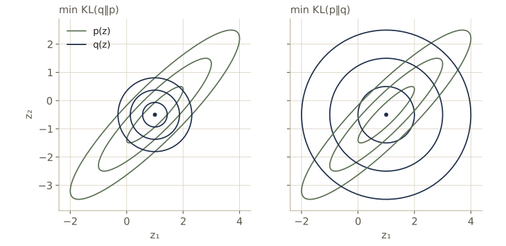
The difference comes from where each divergence is expensive. In \(\mathrm{KL}(q \Vert p) = -\int q \ln (p/q)\), the integrand is large wherever \(q\) has mass and \(p\) is tiny, so the minimizer keeps \(q\) small wherever \(p\) is small: it is zero-forcing, and it tends to be too compact. In \(\mathrm{KL}(p \Vert q)\) the roles swap: any region where \(p\) has mass and \(q\) is near zero is heavily penalized, so the minimizer is zero-avoiding and spreads \(q\) to cover all of \(p\).
Watch out. Mean-field variational inference minimizes \(\mathrm{KL}(q \Vert p)\), so its posteriors are systematically too narrow when the true posterior has correlations between the factors. The means are often good; the error bars are often too small. Keep this in mind whenever you report a variational credible interval.
One mode or all of them
The contrast is sharper when the target has several modes, which real posteriors often do (the mixture models of module 09 have one posterior mode per relabeling of the components). Approximate a two-component mixture \(p(z)\) in one dimension by a single Gaussian \(q(z) = \mathcal{N}(z \mid m, s^2)\). For \(\mathrm{KL}(p \Vert q)\) the answer is to match the mean and variance of \(p\), as we will prove for the whole exponential family in the section on expectation propagation. For \(\mathrm{KL}(q \Vert p)\) there is no closed form, so we evaluate it on a grid of \((m, s)\) values, with the integral over \(z\) done numerically, and look for local minima.
def normal_pdf(z, m, v):
    return np.exp(-0.5 * (z - m) ** 2 / v) / np.sqrt(2 * np.pi * v)

z = np.linspace(-9, 9, 3601); dz = z[1] - z[0]
p_mix = 0.6 * normal_pdf(z, -2.2, 0.6 ** 2) + 0.4 * normal_pdf(z, 2.2, 0.6 ** 2)
ln_p = np.log(p_mix)

# KL(p||q) is minimized by matching the first two moments of p
m_fwd = np.sum(z * p_mix) * dz
s_fwd = np.sqrt(np.sum((z - m_fwd) ** 2 * p_mix) * dz)

def kl_q_p(m, s):
    """KL(q||p) for q = N(m, s^2): -entropy(q) - E_q[ln p], by quadrature over z."""
    q = normal_pdf(z[None, :], m[:, None], s ** 2)
    return -0.5 * np.log(2 * np.pi * np.e * s ** 2) - (q * ln_p).sum(axis=1) * dz

ms = np.linspace(-4, 4, 401)
ss = np.linspace(0.2, 3.0, 141)
KLgrid = np.array([kl_q_p(ms, s) for s in ss])          # rows: s, columns: m

# interior grid points that are lower than all eight neighbors
R, C = KLgrid.shape
inner = KLgrid[1:-1, 1:-1]
is_min = np.ones_like(inner, dtype=bool)
for di in (-1, 0, 1):
    for dj in (-1, 0, 1):
        if di or dj:
            is_min &= inner < KLgrid[1 + di:R - 1 + di, 1 + dj:C - 1 + dj]
print(f"moment matching (min KL(p||q)):  m = {m_fwd:.3f}, s = {s_fwd:.3f}")
for i, j in zip(*np.nonzero(is_min)):
    m_, s_, kl = ms[j + 1], ss[i + 1], KLgrid[i + 1, j + 1]
    print(f"local min of KL(q||p):           m = {m_:.3f}, s = {s_:.3f}, "
          f"KL(q||p) = {kl:.3f}")
moment matching (min KL(p||q)):  m = -0.440, s = 2.237
local min of KL(q||p):           m = -2.200, s = 0.600, KL(q||p) = 0.511
local min of KL(q||p):           m = 2.200, s = 0.600, KL(q||p) = 0.916
local min of KL(q||p):           m = -0.360, s = 1.900, KL(q||p) = 1.487
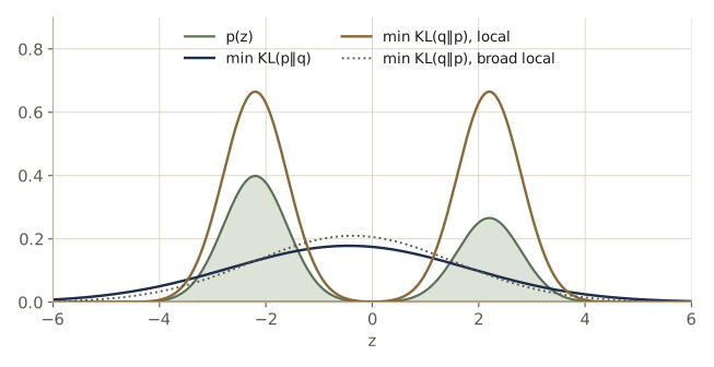
The moment-matched Gaussian sits between the modes, where \(p\) is almost zero, and is very wide. The reverse divergence has three local minima. Two of them lock onto one mode each, with a width close to that mode’s own width of 0.6, and the one on the heavier mode has the lowest divergence of all. The third straddles both modes; it is a genuine local minimum, but its divergence is far larger, because it puts a lot of mass in the trough. For a mixture posterior this is the behavior we want: each mode of a mixture posterior is a perfectly good explanation of the data, and their average usually is not. Variational inference picks one mode and describes it well. We will have to remember that it ignored the others when we compare models later.
The alpha family
The two KL divergences are the ends of a one-parameter family. For \(-\infty < \alpha < \infty\), the alpha divergence is
\[D_\alpha(p \Vert q) = \frac{4}{1 - \alpha^2} \left( 1 - \int p(x)^{(1 + \alpha)/2} \, q(x)^{(1 - \alpha)/2} \, \mathrm{d}x \right).\]It is nonnegative and zero only when \(p = q\). As \(\alpha \to 1\) it tends to \(\mathrm{KL}(p \Vert q)\), and as \(\alpha \to -1\) to \(\mathrm{KL}(q \Vert p)\) (exercise 2). For \(\alpha \le -1\) the minimizing \(q\) is zero-forcing and tends to hug the largest mode; for \(\alpha \ge 1\) it is zero-avoiding and stretches over all of \(p\). The midpoint \(\alpha = 0\) gives a symmetric divergence, four times one minus the integral of \(\sqrt{p q}\), which is a multiple of the squared Hellinger distance \(\int (\sqrt{p} - \sqrt{q})^2 \, \mathrm{d}x\); the square root of that is a true metric. The alpha family is the backbone of a general theory that derives many approximate inference algorithms, including the two in this module, from one objective (see Going further).
Example: a Gaussian with unknown mean and precision
Now a real inference problem, small enough that we also know the exact answer. We observe \(\mathcal{D} = \{x_1, \dots, x_N\}\) drawn independently from \(\mathcal{N}(x \mid \mu, \tau^{-1})\) with both the mean \(\mu\) and the precision \(\tau\) unknown. As in module 02, the conjugate prior is normal-gamma:
\[p(\mu \mid \tau) = \mathcal{N}\!\left(\mu \mid \mu_0, (\lambda_0 \tau)^{-1}\right), \qquad p(\tau) = \operatorname{Gam}(\tau \mid a_0, b_0).\]The exact posterior is normal-gamma too, and it does not factorize: the conditional variance of \(\mu\) given \(\tau\) is \(1/((\lambda_0 + N)\tau)\), so \(\mu\) and \(\tau\) are dependent. We approximate it anyway by \(q(\mu, \tau) = q_\mu(\mu)\, q_\tau(\tau)\), to see the machinery at work.
The factor for \(\mu\). The log joint is \(\ln p(\mathcal{D} \mid \mu, \tau) + \ln p(\mu \mid \tau) + \ln p(\tau)\). The terms involving \(\mu\) are
\[\ln q_\mu^\star(\mu) = -\frac{\mathbb{E}[\tau]}{2} \left( \lambda_0 (\mu - \mu_0)^2 + \sum_{n=1}^{N} (x_n - \mu)^2 \right) + \text{const}.\]A quadratic in \(\mu\) again, so \(q_\mu^\star(\mu) = \mathcal{N}(\mu \mid \mu_N, \lambda_N^{-1})\) with
\[\mu_N = \frac{\lambda_0 \mu_0 + N \bar{x}}{\lambda_0 + N}, \qquad \lambda_N = (\lambda_0 + N)\, \mathbb{E}[\tau].\]The factor for \(\tau\). Collect every term that involves \(\tau\). The likelihood contributes \(\frac{N}{2} \ln \tau\), the conditional prior on \(\mu\) contributes \(\frac{1}{2} \ln \tau\) from its normalizer, and the gamma prior contributes \((a_0 - 1) \ln \tau - b_0 \tau\):
\[\begin{aligned} \ln q_\tau^\star(\tau) &= \left( a_0 - 1 + \frac{N + 1}{2} \right) \ln \tau \\ &\quad - \tau \left( b_0 + \frac{1}{2} \mathbb{E}_\mu\!\left[ \sum_{n=1}^{N} (x_n - \mu)^2 + \lambda_0 (\mu - \mu_0)^2 \right] \right) + \text{const}. \end{aligned}\]That is the log of a gamma density, \(q_\tau^\star(\tau) = \operatorname{Gam}(\tau \mid a_N, b_N)\) with
\[a_N = a_0 + \frac{N + 1}{2}, \qquad b_N = b_0 + \frac{1}{2} \mathbb{E}_\mu\!\left[ \sum_{n=1}^{N} (x_n - \mu)^2 + \lambda_0 (\mu - \mu_0)^2 \right].\]The expectation needs only the first two moments of \(q_\mu\): \(\mathbb{E}[(x_n - \mu)^2] = (x_n - \mu_N)^2 + \lambda_N^{-1}\). And the update for \(q_\mu\) needs only \(\mathbb{E}[\tau] = a_N / b_N\). So the whole algorithm is: guess \(\mathbb{E}[\tau]\), then alternate the two updates.
The \(\frac{1}{2} \ln \tau\) from the normalizer of \(p(\mu \mid \tau)\) is easy to drop, and dropping it changes \(a_N\) by one half. In general, when a density’s normalizer depends on another variable, that normalizer belongs in the other variable’s update.
def vi_normal_gamma(x, mu0, lam0, a0, b0, E_tau=1.0, iters=100, tol=1e-12,
                    trace=False):
    """Mean-field q(mu) q(tau) for a Gaussian with unknown mean and precision."""
    N, xbar = len(x), x.mean()
    muN = (lam0 * mu0 + N * xbar) / (lam0 + N)     # does not change between sweeps
    aN = a0 + (N + 1) / 2                          # does not change either
    for it in range(1, iters + 1):
        lamN = (lam0 + N) * E_tau                  # update q(mu)
        E_sq = np.sum((x - muN) ** 2) + lam0 * (muN - mu0) ** 2 + (N + lam0) / lamN
        bN = b0 + 0.5 * E_sq                       # update q(tau)
        E_tau_new = aN / bN
        if trace and it <= 4:
            print(f"sweep {it}: E[mu] = {muN:.4f}, sd[mu] = {lamN ** -0.5:.4f},"
                  f" E[tau] = {E_tau_new:.4f}")
        if abs(E_tau_new - E_tau) < tol:
            break
        E_tau = E_tau_new
    return muN, lamN, aN, bN, it

rng = np.random.default_rng(10)
x_g = rng.normal(0.6, 0.7, size=10)          # true mu = 0.6, tau = 1/0.49 = 2.04
mu0, lam0, a0, b0 = 0.0, 1.0, 1.0, 1.0
muN, lamN, aN, bN, n_it = vi_normal_gamma(x_g, mu0, lam0, a0, b0, E_tau=0.3,
                                          trace=True)
print(f"converged after {n_it} sweeps")
sweep 1: E[mu] = 0.4984, sd[mu] = 0.5505, E[tau] = 1.6827
sweep 2: E[mu] = 0.4984, sd[mu] = 0.2324, E[tau] = 2.6071
sweep 3: E[mu] = 0.4984, sd[mu] = 0.1867, E[tau] = 2.7221
sweep 4: E[mu] = 0.4984, sd[mu] = 0.1827, E[tau] = 2.7314
converged after 13 sweeps
Starting from a poor guess \(\mathbb{E}[\tau] = 0.3\), the updates settle within a few sweeps. Now the exact posterior, for comparison. It is normal-gamma with \(\mu_N\) as above and
\[\lambda_N^{\text{ex}} = \lambda_0 + N, \quad a_N^{\text{ex}} = a_0 + \frac{N}{2}, \quad b_N^{\text{ex}} = b_0 + \frac{1}{2} \sum_n (x_n - \bar{x})^2 + \frac{\lambda_0 N (\bar{x} - \mu_0)^2}{2 (\lambda_0 + N)}.\]Its marginal for \(\mu\) is a Student’s t with variance \(b_N^{\text{ex}} / (\lambda_N^{\text{ex}} (a_N^{\text{ex}} - 1))\). We also compute the exact log evidence and the variational lower bound, whose difference should be the KL divergence from \(q\) to the exact posterior.
N, xbar = len(x_g), x_g.mean()
lam_ex, a_ex = lam0 + N, a0 + N / 2
b_ex = (b0 + 0.5 * np.sum((x_g - xbar) ** 2)
        + lam0 * N * (xbar - mu0) ** 2 / (2 * (lam0 + N)))
ln_evidence = (gammaln(a_ex) - gammaln(a0) + a0 * np.log(b0) - a_ex * np.log(b_ex)
               + 0.5 * np.log(lam0 / lam_ex) - 0.5 * N * np.log(2 * np.pi))

def elbo_normal_gamma(x, mu0, lam0, a0, b0, muN, lamN, aN, bN):
    """L(q) = E[ln p(D, mu, tau)] - E[ln q(mu)] - E[ln q(tau)] for factorized q."""
    N = len(x)
    E_tau, E_ln_tau = aN / bN, digamma(aN) - np.log(bN)
    E_sq_data = np.sum((x - muN) ** 2) + N / lamN          # E[sum (x_n - mu)^2]
    E_sq_prior = (muN - mu0) ** 2 + 1 / lamN                # E[(mu - mu0)^2]
    lik = 0.5 * N * (E_ln_tau - np.log(2 * np.pi)) - 0.5 * E_tau * E_sq_data
    prior_mu = (0.5 * (np.log(lam0) + E_ln_tau - np.log(2 * np.pi))
                - 0.5 * lam0 * E_tau * E_sq_prior)
    prior_tau = a0 * np.log(b0) - gammaln(a0) + (a0 - 1) * E_ln_tau - b0 * E_tau
    H_mu = 0.5 * np.log(2 * np.pi * np.e / lamN)
    H_tau = gammaln(aN) - (aN - 1) * digamma(aN) - np.log(bN) + aN
    return lik + prior_mu + prior_tau + H_mu + H_tau

L_vi = elbo_normal_gamma(x_g, mu0, lam0, a0, b0, muN, lamN, aN, bN)
print(f"E[mu]:   VI {muN:.4f}   exact {muN:.4f}")
sd_mu_exact = np.sqrt(b_ex / (lam_ex * (a_ex - 1)))      # Student's t marginal
print(f"sd[mu]:  VI {lamN ** -0.5:.4f}   exact {sd_mu_exact:.4f}")
print(f"E[tau]:  VI {aN / bN:.4f}   exact {a_ex / b_ex:.4f}")
print(f"sd[tau]: VI {np.sqrt(aN) / bN:.4f}   exact {np.sqrt(a_ex) / b_ex:.4f}")
print(f"lower bound {L_vi:.4f} <= ln p(D) = {ln_evidence:.4f}")
print(f"KL(q||p) = ln p(D) - L = {ln_evidence - L_vi:.4f}")
E[mu]:   VI 0.4984   exact 0.4984
sd[mu]:  VI 0.1824   exact 0.1998
E[tau]:  VI 2.7322   exact 2.7322
sd[tau]: VI 1.0716   exact 1.1154
lower bound -10.3619 <= ln p(D) = -10.3208
KL(q||p) = ln p(D) - L = 0.0411
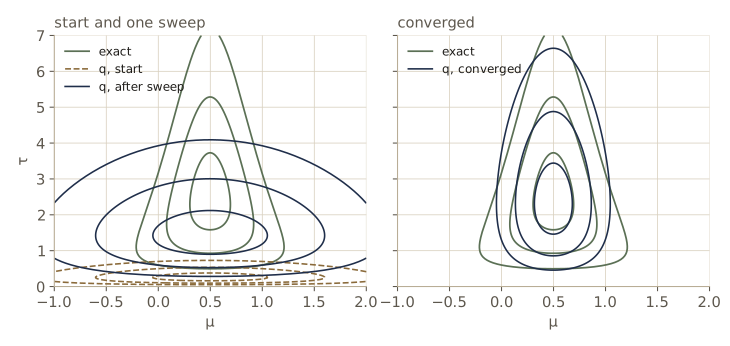
The posterior means of \(\mu\) and of \(\tau\) are both exact; the first is clear from the update, and the second is no accident either (exercise 4). The standard deviations are smaller than the exact ones, the too-compact behavior we predicted, though here the factorization costs little: the KL divergence between \(q\) and the true posterior is only about 0.04 nats. The figure shows the same thing in the \((\mu, \tau)\) plane.
Model comparison
Variational inference also gives approximate posterior probabilities over a set of candidate models \(m\) with prior probabilities \(p(m)\). Different models may have different latent variables, so \(q\) over \(\mathbf{Z}\) must depend on the model: we take \(q(\mathbf{Z}, m) = q(\mathbf{Z} \mid m)\, q(m)\). The same decomposition as before, now with a sum over \(m\), shows that
\[\mathcal{L} = \sum_m q(m) \left( \mathcal{L}_m + \ln \frac{p(m)}{q(m)} \right), \qquad \mathcal{L}_m = \int q(\mathbf{Z} \mid m) \ln \frac{p(\mathbf{X}, \mathbf{Z} \mid m)}{q(\mathbf{Z} \mid m)} \, \mathrm{d}\mathbf{Z},\]is a lower bound on \(\ln p(\mathbf{X})\) (exercise 3). In practice we fit each model separately, maximizing its own bound \(\mathcal{L}_m\) over \(q(\mathbf{Z} \mid m)\), and then maximize over \(q(m)\) with a Lagrange multiplier for normalization, which gives
\[q(m) \propto p(m) \exp(\mathcal{L}_m).\]This is Bayes’ rule for models with each log evidence replaced by its lower bound. We use it for the number of mixture components and the degree of a polynomial below.
The variational mixture of Gaussians
Here is the model that shows off variational inference best. In module 09 we fit Gaussian mixtures by maximum likelihood with EM, and met its problems: the likelihood is unbounded when a component collapses onto one point, and it always prefers more components, so it cannot tell us how many to use. A Bayesian treatment fixes both, and the variational algorithm that implements it costs about as much as EM.
The model
Each data point \(\mathbf{x}_n \in \mathbb{R}^D\) has a latent 1-of-\(K\) vector \(\mathbf{z}_n\) that says which component generated it. As in module 09, but writing each component with its precision matrix \(\boldsymbol{\Lambda}_k\) instead of its covariance (the algebra is lighter),
\[p(\mathbf{Z} \mid \boldsymbol{\pi}) = \prod_{n=1}^{N} \prod_{k=1}^{K} \pi_k^{z_{nk}}, \qquad p(\mathbf{X} \mid \mathbf{Z}, \boldsymbol{\mu}, \boldsymbol{\Lambda}) = \prod_{n=1}^{N} \prod_{k=1}^{K} \mathcal{N}\!\left(\mathbf{x}_n \mid \boldsymbol{\mu}_k, \boldsymbol{\Lambda}_k^{-1}\right)^{z_{nk}}.\]Now the parameters get conjugate priors (module 02). The mixing coefficients get a symmetric Dirichlet, and each component’s mean and precision a Gaussian–Wishart:
\[\begin{aligned} p(\boldsymbol{\pi}) &= \operatorname{Dir}(\boldsymbol{\pi} \mid \alpha_0) = C(\boldsymbol{\alpha}_0) \prod_{k=1}^{K} \pi_k^{\alpha_0 - 1}, \\ p(\boldsymbol{\mu}_k, \boldsymbol{\Lambda}_k) &= \mathcal{N}\!\left(\boldsymbol{\mu}_k \mid \mathbf{m}_0, (\beta_0 \boldsymbol{\Lambda}_k)^{-1}\right) \mathcal{W}(\boldsymbol{\Lambda}_k \mid \mathbf{W}_0, \nu_0). \end{aligned}\]Here \(C(\boldsymbol{\alpha})\) is the Dirichlet normalizer, \(\Gamma(\hat{\alpha}) / \prod_k \Gamma(\alpha_k)\) with \(\hat{\alpha} = \sum_k \alpha_k\), and \(\mathcal{W}(\boldsymbol{\Lambda} \mid \mathbf{W}, \nu)\) is the Wishart density over symmetric positive definite matrices, with mean \(\nu \mathbf{W}\) and normalizer \(B(\mathbf{W}, \nu)\) (Bishop, Appendix B). The number \(\alpha_0\) acts like a prior count of points in each component: a small \(\alpha_0\) lets the data decide, and \(\alpha_0 < 1\) actively favors solutions in which some mixing coefficients are near zero. The joint distribution of everything is
\[p(\mathbf{X}, \mathbf{Z}, \boldsymbol{\pi}, \boldsymbol{\mu}, \boldsymbol{\Lambda}) = p(\mathbf{X} \mid \mathbf{Z}, \boldsymbol{\mu}, \boldsymbol{\Lambda})\, p(\mathbf{Z} \mid \boldsymbol{\pi})\, p(\boldsymbol{\pi})\, p(\boldsymbol{\mu} \mid \boldsymbol{\Lambda})\, p(\boldsymbol{\Lambda}).\]As a directed graph (module 08): \(\boldsymbol{\pi}\) points to each \(\mathbf{z}_n\); \(\mathbf{z}_n\), \(\boldsymbol{\mu}\), and \(\boldsymbol{\Lambda}\) point to \(\mathbf{x}_n\); and \(\boldsymbol{\Lambda}\) points to \(\boldsymbol{\mu}\), because the prior variance of the means scales with the component covariance. The \(\mathbf{z}_n\) live inside the plate over data points, so their number grows with \(N\); the parameters sit outside. From the graph’s point of view, the distinction between “latent variables” and “parameters” is only this bookkeeping.
The variational distribution
The only assumption we make is that the latent assignments and the parameters are independent under \(q\):
\[q(\mathbf{Z}, \boldsymbol{\pi}, \boldsymbol{\mu}, \boldsymbol{\Lambda}) = q(\mathbf{Z})\, q(\boldsymbol{\pi}, \boldsymbol{\mu}, \boldsymbol{\Lambda}).\]Everything else, including the functional form of every factor and any further independence, will come out of the general result.
The factor over assignments. Keep the terms of the log joint that involve \(\mathbf{Z}\) and average over the parameters:
\[\begin{aligned} \ln q^\star(\mathbf{Z}) &= \mathbb{E}_{\boldsymbol{\pi}}[\ln p(\mathbf{Z} \mid \boldsymbol{\pi})] + \mathbb{E}_{\boldsymbol{\mu}, \boldsymbol{\Lambda}}[\ln p(\mathbf{X} \mid \mathbf{Z}, \boldsymbol{\mu}, \boldsymbol{\Lambda})] + \text{const} \\ &= \sum_{n=1}^{N} \sum_{k=1}^{K} z_{nk} \ln \rho_{nk} + \text{const}, \end{aligned}\]because both log densities are linear in the \(z_{nk}\). The coefficient of \(z_{nk}\) is
\[\begin{aligned} \ln \rho_{nk} &= \mathbb{E}[\ln \pi_k] + \tfrac{1}{2} \mathbb{E}[\ln \det \boldsymbol{\Lambda}_k] - \tfrac{D}{2} \ln (2\pi) \\ &\quad - \tfrac{1}{2} \mathbb{E}_{\boldsymbol{\mu}_k, \boldsymbol{\Lambda}_k}\!\left[ (\mathbf{x}_n - \boldsymbol{\mu}_k)^{\mathrm{T}} \boldsymbol{\Lambda}_k (\mathbf{x}_n - \boldsymbol{\mu}_k) \right]. \end{aligned}\]Exponentiating, \(q^\star(\mathbf{Z}) \propto \prod_n \prod_k \rho_{nk}^{z_{nk}}\). Each \(\mathbf{z}_n\) has exactly one entry equal to 1, so normalizing point by point gives
\[q^\star(\mathbf{Z}) = \prod_{n=1}^{N} \prod_{k=1}^{K} r_{nk}^{z_{nk}}, \qquad r_{nk} = \frac{\rho_{nk}}{\sum_{j} \rho_{nj}}, \qquad \mathbb{E}[z_{nk}] = r_{nk}.\]These \(r_{nk}\) play exactly the role of the responsibilities in EM. Note that we did not ask for \(q(\mathbf{Z})\) to factorize over data points; it did anyway.
The factor over parameters. We will need three statistics of the data weighted by the responsibilities, the same ones as in EM:
\[N_k = \sum_{n=1}^{N} r_{nk}, \quad \bar{\mathbf{x}}_k = \frac{1}{N_k} \sum_{n=1}^{N} r_{nk} \mathbf{x}_n, \quad \mathbf{S}_k = \frac{1}{N_k} \sum_{n=1}^{N} r_{nk} (\mathbf{x}_n - \bar{\mathbf{x}}_k)(\mathbf{x}_n - \bar{\mathbf{x}}_k)^{\mathrm{T}}.\]The terms of the log joint involving the parameters are
\[\begin{aligned} \ln q^\star(\boldsymbol{\pi}, \boldsymbol{\mu}, \boldsymbol{\Lambda}) &= \ln p(\boldsymbol{\pi}) + \mathbb{E}_{\mathbf{Z}}[\ln p(\mathbf{Z} \mid \boldsymbol{\pi})] \\ &\quad + \sum_{k=1}^{K} \left\{ \ln p(\boldsymbol{\mu}_k, \boldsymbol{\Lambda}_k) + \sum_{n=1}^{N} r_{nk} \ln \mathcal{N}\!\left(\mathbf{x}_n \mid \boldsymbol{\mu}_k, \boldsymbol{\Lambda}_k^{-1}\right) \right\} + \text{const}. \end{aligned}\]This is a sum of a part involving only \(\boldsymbol{\pi}\) and, for each \(k\), a part involving only \((\boldsymbol{\mu}_k, \boldsymbol{\Lambda}_k)\). So the optimal factor splits further, \(q^\star(\boldsymbol{\pi}) \prod_k q^\star(\boldsymbol{\mu}_k, \boldsymbol{\Lambda}_k)\), without our assuming it. The \(\boldsymbol{\pi}\) part is \(\sum_k (\alpha_0 - 1 + N_k) \ln \pi_k\), the log of a Dirichlet:
\[q^\star(\boldsymbol{\pi}) = \operatorname{Dir}(\boldsymbol{\pi} \mid \boldsymbol{\alpha}), \qquad \alpha_k = \alpha_0 + N_k.\]The \(k\)th component’s part is the log of its Gaussian–Wishart prior plus a Gaussian log likelihood of the data with weights \(r_{nk}\). By conjugacy (the same computation as a posterior with \(N_k\) “points”; exercise 5) it is again Gaussian–Wishart:
\[q^\star(\boldsymbol{\mu}_k, \boldsymbol{\Lambda}_k) = \mathcal{N}\!\left(\boldsymbol{\mu}_k \mid \mathbf{m}_k, (\beta_k \boldsymbol{\Lambda}_k)^{-1}\right) \mathcal{W}(\boldsymbol{\Lambda}_k \mid \mathbf{W}_k, \nu_k),\] \[\begin{aligned} \beta_k &= \beta_0 + N_k, \qquad \mathbf{m}_k = \frac{1}{\beta_k} (\beta_0 \mathbf{m}_0 + N_k \bar{\mathbf{x}}_k), \qquad \nu_k = \nu_0 + N_k, \\ \mathbf{W}_k^{-1} &= \mathbf{W}_0^{-1} + N_k \mathbf{S}_k + \frac{\beta_0 N_k}{\beta_0 + N_k} (\bar{\mathbf{x}}_k - \mathbf{m}_0)(\bar{\mathbf{x}}_k - \mathbf{m}_0)^{\mathrm{T}}. \end{aligned}\]Each update is the prior’s parameters plus data counts, like the M step of EM with the prior acting as pseudo-observations.
The expectations that close the loop. The responsibilities need three averages under the current parameter factors, all standard properties of the Dirichlet and Wishart (exercise 6):
\[\begin{aligned} \mathbb{E}_{\boldsymbol{\mu}_k, \boldsymbol{\Lambda}_k}\!\left[ (\mathbf{x}_n - \boldsymbol{\mu}_k)^{\mathrm{T}} \boldsymbol{\Lambda}_k (\mathbf{x}_n - \boldsymbol{\mu}_k) \right] &= D \beta_k^{-1} + \nu_k (\mathbf{x}_n - \mathbf{m}_k)^{\mathrm{T}} \mathbf{W}_k (\mathbf{x}_n - \mathbf{m}_k), \\ \ln \tilde{\Lambda}_k \equiv \mathbb{E}[\ln \det \boldsymbol{\Lambda}_k] &= \sum_{i=1}^{D} \psi\!\left( \frac{\nu_k + 1 - i}{2} \right) + D \ln 2 + \ln \det \mathbf{W}_k, \\ \ln \tilde{\pi}_k \equiv \mathbb{E}[\ln \pi_k] &= \psi(\alpha_k) - \psi(\hat{\alpha}), \end{aligned}\]where \(\psi\) is the digamma function, the derivative of \(\ln \Gamma\). Substituting,
\[r_{nk} \propto \tilde{\pi}_k \, \tilde{\Lambda}_k^{1/2} \exp\!\left\{ -\frac{D}{2 \beta_k} - \frac{\nu_k}{2} (\mathbf{x}_n - \mathbf{m}_k)^{\mathrm{T}} \mathbf{W}_k (\mathbf{x}_n - \mathbf{m}_k) \right\}.\]Compare the EM responsibilities,
\[r_{nk} \propto \pi_k \det(\boldsymbol{\Lambda}_k)^{1/2} \exp\!\left\{ -\frac{1}{2} (\mathbf{x}_n - \boldsymbol{\mu}_k)^{\mathrm{T}} \boldsymbol{\Lambda}_k (\mathbf{x}_n - \boldsymbol{\mu}_k) \right\}.\]The shape is the same; the point estimates are replaced by averages over the posterior, and there is an extra penalty \(D / (2\beta_k)\) for uncertainty about the mean. So the algorithm alternates a variational E step (compute the three expectations and the responsibilities) and a variational M step (recompute \(N_k\), \(\bar{\mathbf{x}}_k\), \(\mathbf{S}_k\) and then \(\boldsymbol{\alpha}\), \(\beta_k\), \(\mathbf{m}_k\), \(\mathbf{W}_k\), \(\nu_k\)).
The lower bound
We also want the bound itself, to monitor convergence and to compare models. With every expectation taken under the current \(q\),
\[\begin{aligned} \mathcal{L} &= \mathbb{E}[\ln p(\mathbf{X} \mid \mathbf{Z}, \boldsymbol{\mu}, \boldsymbol{\Lambda})] + \mathbb{E}[\ln p(\mathbf{Z} \mid \boldsymbol{\pi})] + \mathbb{E}[\ln p(\boldsymbol{\pi})] + \mathbb{E}[\ln p(\boldsymbol{\mu}, \boldsymbol{\Lambda})] \\ &\quad - \mathbb{E}[\ln q(\mathbf{Z})] - \mathbb{E}[\ln q(\boldsymbol{\pi})] - \mathbb{E}[\ln q(\boldsymbol{\mu}, \boldsymbol{\Lambda})]. \end{aligned}\]Each term is a standard expectation (exercise 7). In terms of the quantities above:
\[\begin{aligned} \mathbb{E}[\ln p(\mathbf{X} \mid \mathbf{Z}, \boldsymbol{\mu}, \boldsymbol{\Lambda})] &= \frac{1}{2} \sum_{k} N_k \Big\{ \ln \tilde{\Lambda}_k - D \beta_k^{-1} - \nu_k \operatorname{tr}(\mathbf{S}_k \mathbf{W}_k) \\ &\qquad\qquad - \nu_k (\bar{\mathbf{x}}_k - \mathbf{m}_k)^{\mathrm{T}} \mathbf{W}_k (\bar{\mathbf{x}}_k - \mathbf{m}_k) - D \ln (2\pi) \Big\}, \\ \mathbb{E}[\ln p(\mathbf{Z} \mid \boldsymbol{\pi})] &= \sum_{n} \sum_{k} r_{nk} \ln \tilde{\pi}_k, \\ \mathbb{E}[\ln p(\boldsymbol{\pi})] &= \ln C(\boldsymbol{\alpha}_0) + (\alpha_0 - 1) \sum_k \ln \tilde{\pi}_k, \\ \mathbb{E}[\ln p(\boldsymbol{\mu}, \boldsymbol{\Lambda})] &= \frac{1}{2} \sum_{k} \Big\{ D \ln \frac{\beta_0}{2\pi} + \ln \tilde{\Lambda}_k - \frac{D \beta_0}{\beta_k} \\ &\qquad\qquad - \beta_0 \nu_k (\mathbf{m}_k - \mathbf{m}_0)^{\mathrm{T}} \mathbf{W}_k (\mathbf{m}_k - \mathbf{m}_0) \Big\} \\ &\quad + K \ln B(\mathbf{W}_0, \nu_0) + \frac{\nu_0 - D - 1}{2} \sum_k \ln \tilde{\Lambda}_k \\ &\quad - \frac{1}{2} \sum_k \nu_k \operatorname{tr}(\mathbf{W}_0^{-1} \mathbf{W}_k), \\ \mathbb{E}[\ln q(\mathbf{Z})] &= \sum_{n} \sum_{k} r_{nk} \ln r_{nk}, \\ \mathbb{E}[\ln q(\boldsymbol{\pi})] &= \sum_k (\alpha_k - 1) \ln \tilde{\pi}_k + \ln C(\boldsymbol{\alpha}), \\ \mathbb{E}[\ln q(\boldsymbol{\mu}, \boldsymbol{\Lambda})] &= \sum_k \left\{ \frac{1}{2} \ln \tilde{\Lambda}_k + \frac{D}{2} \ln \frac{\beta_k}{2\pi} - \frac{D}{2} - \mathrm{H}[q(\boldsymbol{\Lambda}_k)] \right\}, \end{aligned}\]where \(\mathrm{H}[q(\boldsymbol{\Lambda}_k)]\) is the entropy of the Wishart factor,
\[\mathrm{H}[q(\boldsymbol{\Lambda}_k)] = -\ln B(\mathbf{W}_k, \nu_k) - \frac{\nu_k - D - 1}{2} \ln \tilde{\Lambda}_k + \frac{\nu_k D}{2},\]and
\[\ln B(\mathbf{W}, \nu) = -\frac{\nu}{2} \ln \det \mathbf{W} - \frac{\nu D}{2} \ln 2 - \frac{D (D - 1)}{4} \ln \pi - \sum_{i=1}^{D} \ln \Gamma\!\left( \frac{\nu + 1 - i}{2} \right).\]The terms with \(\ln q\) are negative entropies. It is a long formula, but every piece is one line of code, and the payoff is a strong test: after every full sweep the bound must not decrease. A sign error or a wrong factor in any update equation almost always shows up as a drop.
Implementation
We implement the two steps and the bound as separate functions that follow the equations above.
def ln_wishart_B(W, nu):
    """log of the Wishart normalizer B(W, nu)."""
    D = W.shape[0]
    i = np.arange(1, D + 1)
    return (-0.5 * nu * np.linalg.slogdet(W)[1] - 0.5 * nu * D * np.log(2)
            - 0.25 * D * (D - 1) * np.log(np.pi) - gammaln(0.5 * (nu + 1 - i)).sum())

def ln_dirichlet_C(alpha):
    """log of the Dirichlet normalizer C(alpha)."""
    return gammaln(alpha.sum()) - gammaln(alpha).sum()

def vb_m_step(X, r, prior):
    """Variational M step: q(pi) = Dir(alpha), q(mu_k, Lam_k) = Gaussian-Wishart."""
    N, D = X.shape
    b0, m0 = prior["beta0"], prior["m0"]
    Nk = r.sum(axis=0) + 1e-10                  # floor keeps empty components finite
    xbar = (r.T @ X) / Nk[:, None]
    dx = X[:, None] - xbar                                            # (N, K, D)
    S = np.einsum('nk,nki,nkj->kij', r, dx, dx) / Nk[:, None, None]
    alpha = prior["alpha0"] + Nk
    beta = b0 + Nk
    m = (b0 * m0 + Nk[:, None] * xbar) / beta[:, None]
    nu = prior["nu0"] + Nk
    dm = xbar - m0
    W_inv = (np.linalg.inv(prior["W0"]) + Nk[:, None, None] * S
             + (b0 * Nk / (b0 + Nk))[:, None, None] * np.einsum('ki,kj->kij', dm, dm))
    W = np.linalg.inv(W_inv)                    # K small D-by-D matrices; we need W
    return dict(alpha=alpha, beta=beta, m=m, W=W, nu=nu, Nk=Nk, xbar=xbar, S=S)

def vb_expectations(post):
    """ln tilde-pi_k = E[ln pi_k] and ln tilde-Lambda_k = E[ln det Lam_k]."""
    D = post["m"].shape[1]
    ln_pi = digamma(post["alpha"]) - digamma(post["alpha"].sum())
    i = np.arange(1, D + 1)
    ln_Lam = (digamma(0.5 * (post["nu"][:, None] + 1 - i)).sum(axis=1)
              + D * np.log(2) + np.linalg.slogdet(post["W"])[1])
    return ln_pi, ln_Lam

def vb_e_step(X, post):
    """Variational E step: responsibilities r_nk."""
    N, D = X.shape
    ln_pi, ln_Lam = vb_expectations(post)
    dx = X[:, None, :] - post["m"][None]                                  # (N, K, D)
    maha = np.einsum('nki,kij,nkj->nk', dx, post["W"], dx)
    E_quad = D / post["beta"] + post["nu"] * maha
    ln_rho = ln_pi + 0.5 * ln_Lam - 0.5 * D * np.log(2 * np.pi) - 0.5 * E_quad
    return np.exp(ln_rho - logsumexp(ln_rho, axis=1, keepdims=True))

def vb_bound(X, r, post, prior):
    """The variational lower bound L, term by term."""
    N, D = X.shape
    K = len(post["alpha"])
    a, b, m, W, nu = post["alpha"], post["beta"], post["m"], post["W"], post["nu"]
    Nk, xbar, S = post["Nk"], post["xbar"], post["S"]
    a0, b0, nu0, W0 = prior["alpha0"], prior["beta0"], prior["nu0"], prior["W0"]
    ln_pi, ln_Lam = vb_expectations(post)
    dxm = xbar - m
    dm0 = m - prior["m0"]
    trSW = np.einsum('kij,kji->k', S, W)
    quad_x = np.einsum('ki,kij,kj->k', dxm, W, dxm)
    quad_m = np.einsum('ki,kij,kj->k', dm0, W, dm0)
    ln2pi = np.log(2 * np.pi)
    E_ln_px = 0.5 * np.sum(Nk * (ln_Lam - D / b - nu * trSW - nu * quad_x - D * ln2pi))
    E_ln_pz = np.sum(r * ln_pi)
    E_ln_ppi = ln_dirichlet_C(np.full(K, a0)) + (a0 - 1) * ln_pi.sum()
    E_ln_pmuL = (0.5 * np.sum(D * np.log(b0 / (2 * np.pi)) + ln_Lam - D * b0 / b
                              - b0 * nu * quad_m)
                 + K * ln_wishart_B(W0, nu0)
                 + 0.5 * (nu0 - D - 1) * ln_Lam.sum()
                 - 0.5 * np.sum(nu * np.einsum('ij,kji->k', np.linalg.inv(W0), W)))
    E_ln_qz = np.sum(r * np.log(np.maximum(r, 1e-300)))
    E_ln_qpi = np.sum((a - 1) * ln_pi) + ln_dirichlet_C(a)
    ln_B = np.array([ln_wishart_B(W[k], nu[k]) for k in range(K)])
    H_Lam = -ln_B - 0.5 * (nu - D - 1) * ln_Lam + 0.5 * nu * D     # Wishart entropies
    E_ln_qmuL = np.sum(0.5 * ln_Lam + 0.5 * D * np.log(b / (2 * np.pi))
                       - 0.5 * D - H_Lam)
    return E_ln_px + E_ln_pz + E_ln_ppi + E_ln_pmuL - E_ln_qz - E_ln_qpi - E_ln_qmuL
The driver initializes the responsibilities softly around \(K\) randomly chosen data points and then alternates M step, bound, E step until the bound stops changing.
def vb_gmm(X, K, prior, seed=0, max_iter=1000, tol=1e-7):
    """Coordinate ascent for the variational mixture; returns post, r, bounds, E[pi]."""
    g = np.random.default_rng(seed)
    centers = X[g.choice(len(X), K, replace=False)]
    d2 = ((X[:, None, :] - centers[None]) ** 2).sum(axis=-1)
    r = np.exp(-0.5 * d2 - logsumexp(-0.5 * d2, axis=1, keepdims=True))
    bounds, Epi = [], []
    for it in range(max_iter):
        post = vb_m_step(X, r, prior)
        bounds.append(vb_bound(X, r, post, prior))
        Epi.append(post["alpha"] / post["alpha"].sum())      # E[pi_k] under q(pi)
        if it > 0 and abs(bounds[-1] - bounds[-2]) < tol:
            break
        r = vb_e_step(X, post)
    return post, r, np.array(bounds), np.array(Epi)
Our data: 250 points in two dimensions from three Gaussian clusters of different sizes and shapes. We deliberately fit \(K = 6\) components, twice too many. The prior is broad: \(\alpha_0 = 10^{-3}\), \(\beta_0 = 1\), \(\nu_0 = D\), \(\mathbf{W}_0 = \mathbf{I}\), and \(\mathbf{m}_0\) at the data mean.
rng = np.random.default_rng(7)
true_means = np.array([[-2.0, -1.0], [1.5, 2.0], [2.0, -1.5]])
true_covs = np.array([[[0.6, 0.25], [0.25, 0.4]],
                      [[0.5, -0.2], [-0.2, 0.5]],
                      [[0.3, 0.0], [0.0, 0.7]]])
sizes = [110, 80, 60]
X_gmm = np.vstack([rng.multivariate_normal(m_, C_, size=s)
                   for m_, C_, s in zip(true_means, true_covs, sizes)])
N_gmm, D_gmm = X_gmm.shape

prior = dict(alpha0=1e-3, beta0=1.0, m0=X_gmm.mean(axis=0), W0=np.eye(D_gmm),
             nu0=float(D_gmm))
post, r, bounds, Epi = vb_gmm(X_gmm, K=6, prior=prior, seed=0)
print(f"N = {N_gmm}, stopped after {len(bounds)} iterations")
print("bound never decreased:", bool(np.all(np.diff(bounds) > -1e-9)))
for it in (0, 5, 12, 20, len(bounds) - 1):
    print(f"iter {it:2d}: L = {bounds[it]:9.3f}   E[pi] = {Epi[it]}")
N = 250, stopped after 35 iterations
bound never decreased: True
iter  0: L =  -932.612   E[pi] = [0.1803 0.1544 0.1003 0.1911 0.1427 0.2312]
iter  5: L =  -854.587   E[pi] = [0.1637 0.1907 0.1087 0.2631 0.0244 0.2493]
iter 12: L =  -832.671   E[pi] = [0.1346 0.275  0.0481 0.3067 0.     0.2356]
iter 20: L =  -812.465   E[pi] = [0.0688 0.3241 0.     0.3735 0.     0.2337]
iter 34: L =  -796.188   E[pi] = [0.     0.3243 0.     0.4413 0.     0.2344]
The bound rises at every iteration, which is our check on all of the algebra above. Watch the mixing weights: three of the six components shrink toward zero and stop contributing, and the other three settle on about 0.44, 0.32, and 0.23, close to the true proportions 110/250, 80/250, and 60/250. Here is what the surviving components look like.
alive = Epi[-1] > 0.01
for k in np.nonzero(alive)[0]:
    cov = np.linalg.inv(post["nu"][k] * post["W"][k])     # inverse of E[Lambda_k]
    print(f"component {k}: E[pi] = {Epi[-1][k]:.3f}, N_k = {post['Nk'][k]:5.1f}, "
          f"mean = {post['m'][k]}, var = {np.diag(cov)}")
print(f"unused: N_k = {post['Nk'][~alive]}, "
      f"alpha_k - alpha0 = {post['alpha'][~alive] - prior['alpha0']}")
component 1: E[pi] = 0.324, N_k =  81.1, mean = [1.5155 1.8938], var = [0.423  0.5787]
component 3: E[pi] = 0.441, N_k = 110.3, mean = [-1.8323 -0.9653], var = [0.5671 0.3048]
component 5: E[pi] = 0.234, N_k =  58.6, mean = [ 1.7208 -1.4649], var = [0.2782 0.6864]
unused: N_k = [0. 0. 0.], alpha_k - alpha0 = [0. 0. 0.]
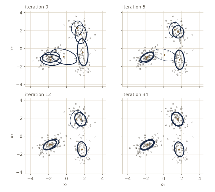
Why do the extra components switch off? A component that explains no points has \(N_k \approx 0\), so every update returns its parameters to the prior: \(\alpha_k \approx \alpha_0\), \(\beta_k \approx \beta_0\), and so on. Keeping it that way costs the bound nothing, while moving it to explain some points would make its posterior differ from its prior, and the bound charges for that difference (the \(\ln q\) terms against the prior terms). This is the same trade-off between fit and complexity that the evidence made in module 03. The posterior mean of a mixing weight is
\[\mathbb{E}[\pi_k] = \frac{\alpha_k}{\hat{\alpha}} = \frac{\alpha_0 + N_k}{K \alpha_0 + N},\]so an unused component has \(\mathbb{E}[\pi_k] \approx \alpha_0 / (K \alpha_0 + N)\): zero for a broad prior with \(\alpha_0 \to 0\), and \(1/K\) if \(\alpha_0 \to \infty\) pins the weights to be equal. The value of \(\alpha_0\) therefore matters. Let us refit with three settings.
for a0_ in (1e-3, 1.0, 10.0):
    _, _, b_a, Epi_a = vb_gmm(X_gmm, K=6, prior=dict(prior, alpha0=a0_), seed=0,
                              max_iter=3000)
    print(f"alpha0 = {a0_:5g}: {len(b_a):3d} iters, E[pi] = {np.sort(Epi_a[-1])[::-1]}")
alpha0 = 0.001:  35 iters, E[pi] = [0.4413 0.3243 0.2344 0.     0.     0.    ]
alpha0 =     1:  44 iters, E[pi] = [0.4343 0.3205 0.2328 0.0041 0.0041 0.0041]
alpha0 =    10: 232 iters, E[pi] = [0.2055 0.1977 0.1968 0.1629 0.1615 0.0755]
With \(\alpha_0 = 1\) the unneeded components keep a small weight but still hold almost no data; with \(\alpha_0 = 10\) the prior insists on six real components, and the fit splits the clusters among them.
Note. Compared with EM from module 09, the variational algorithm has two practical advantages at almost the same cost per iteration. There are no singularities: a component that shrinks onto one point is held back by the Wishart prior, whose \(\mathbf{W}_0^{-1}\) term keeps \(\mathbf{W}_k^{-1}\) positive definite. And there is no overfitting when \(K\) is too large, because unused components switch off. As \(N \to \infty\) with the prior fixed, the posterior factors become sharp and the algorithm reduces to maximum likelihood EM.
The predictive density
For a new point \(\hat{\mathbf{x}}\) the predictive density averages the mixture density over the posterior of the parameters. Replacing that posterior by \(q(\boldsymbol{\pi}) \prod_k q(\boldsymbol{\mu}_k, \boldsymbol{\Lambda}_k)\), the integrals can be done in closed form (exercise 8): averaging a Gaussian over a Gaussian–Wishart gives a multivariate Student’s t, and averaging \(\pi_k\) over the Dirichlet gives \(\alpha_k / \hat{\alpha}\). The result is a mixture of Student’s t distributions,
\[p(\hat{\mathbf{x}} \mid \mathbf{X}) \approx \frac{1}{\hat{\alpha}} \sum_{k=1}^{K} \alpha_k \operatorname{St}\!\left(\hat{\mathbf{x}} \mid \mathbf{m}_k, \mathbf{L}_k, \nu_k + 1 - D\right), \qquad \mathbf{L}_k = \frac{(\nu_k + 1 - D) \beta_k}{1 + \beta_k} \mathbf{W}_k,\]where \(\mathbf{L}_k\) is the precision-like scale matrix of the \(k\)th t distribution and \(\nu_k + 1 - D\) its degrees of freedom. With a lot of data the degrees of freedom are large and each t becomes a Gaussian. Let us score it on fresh data from the same three clusters, against the true density.
def ln_student(X, mu, L, dof):
    """log of the multivariate Student's t St(x | mu, L, dof)."""
    D = X.shape[1]
    dx = X - mu
    delta2 = np.einsum('ni,ij,nj->n', dx, L, dx)
    return (gammaln(0.5 * (dof + D)) - gammaln(0.5 * dof)
            + 0.5 * np.linalg.slogdet(L)[1] - 0.5 * D * np.log(np.pi * dof)
            - 0.5 * (dof + D) * np.log1p(delta2 / dof))

def vb_predictive(Xnew, post):
    D = Xnew.shape[1]
    a = post["alpha"]
    comps = []
    for k in range(len(a)):
        dof = post["nu"][k] + 1 - D
        L = dof * post["beta"][k] / (1 + post["beta"][k]) * post["W"][k]
        comps.append(np.log(a[k] / a.sum()) + ln_student(Xnew, post["m"][k], L, dof))
    return logsumexp(np.array(comps), axis=0)

def ln_gauss(X, mu, cov):
    D = X.shape[1]
    dx = X - mu
    return -0.5 * (np.einsum('ni,ij,nj->n', dx, np.linalg.inv(cov), dx)
                   + np.linalg.slogdet(cov)[1] + D * np.log(2 * np.pi))

labels = rng.choice(3, size=2000, p=np.array(sizes) / N_gmm)
X_test = np.array([rng.multivariate_normal(true_means[c], true_covs[c])
                   for c in labels])
ln_true = logsumexp([np.log(s / N_gmm) + ln_gauss(X_test, true_means[c], true_covs[c])
                     for c, s in enumerate(sizes)], axis=0)
ln_vb = vb_predictive(X_test, post)
print(f"mean test log density: VB {ln_vb.mean():.4f}, true {ln_true.mean():.4f}")
mean test log density: VB -3.1355, true -3.0709
On average the predictive density is within about 0.07 nats per point of the density that generated the data, a small price for having learned it from 250 points.
Determining the number of components
Instead of letting components switch off, we can fit models with \(K = 1, 2, \dots\) and compare their bounds, as in the model comparison section. There is one subtlety. A mixture with \(K\) components has \(K!\) equivalent labelings of its components, so the exact posterior has \(K!\) symmetric copies of each mode. Variational inference, being zero-forcing, fits one copy, so its bound underestimates the log evidence by roughly \(\ln K!\) when the modes are well separated (exercise 9). The fix is to add \(\ln K!\) before comparing.
We use \(\alpha_0 = 1\) here, so that each model really uses its \(K\) components, and take the best of four random starts for each \(K\).
from math import lgamma
prior_K = dict(prior, alpha0=1.0)
print(" K   best L     L + ln K!   starts that reached the best")
for K in range(1, 7):
    Ls = np.array([vb_gmm(X_gmm, K, prior_K, seed=s, max_iter=3000)[2][-1]
                   for s in range(4)])
    best = Ls.max()
    n_best = np.sum(Ls > best - 0.01)
    print(f"{K:2d}  {best:9.2f}  {best + lgamma(K + 1):9.2f}   {n_best} of 4")
 K   best L     L + ln K!   starts that reached the best
 1    -973.57    -973.57   4 of 4
 2    -801.09    -800.39   3 of 4
 3    -783.27    -781.48   3 of 4
 4    -787.65    -784.47   3 of 4
 5    -791.75    -786.96   3 of 4
 6    -795.63    -789.05   4 of 4
Both columns peak at \(K = 3\), the true number of clusters. Maximum likelihood could never do this: its value only grows with \(K\). Notice also that some random starts end in poorer local maxima; in practice we always run several.
A third option sits between the two. Treat \(\boldsymbol{\pi}\) as a parameter to be point-estimated by maximizing the bound, while keeping distributions over everything else. The maximization gives \(\pi_k = N_k / N\), interleaved with the variational updates for the other factors. Components that do not earn their keep get \(\pi_k\) driven to exactly zero and drop out, a form of automatic relevance determination of the kind we met with the relevance vector machine in module 07. This lets one run, started with a large \(K\), prune itself.
Induced factorizations
We assumed only \(q(\mathbf{Z})\, q(\boldsymbol{\pi}, \boldsymbol{\mu}, \boldsymbol{\Lambda})\), and yet the optimal factors came out factorized much further: over data points in \(q(\mathbf{Z})\), between \(\boldsymbol{\pi}\) and the component parameters, and across components. These induced factorizations come from the conditional independences of the true model, and it pays to find them before implementing anything; storing a full joint distribution where a product of small ones would do wastes memory and time.
There is a quick graphical test. Suppose we assume \(q(\mathbf{A}, \mathbf{B}, \mathbf{C}) = q(\mathbf{A}, \mathbf{B})\, q(\mathbf{C})\). The optimal factor is
\[\ln q^\star(\mathbf{A}, \mathbf{B}) = \mathbb{E}_{\mathbf{C}}[\ln p(\mathbf{A}, \mathbf{B} \mid \mathbf{X}, \mathbf{C})] + \text{const},\]and it splits into a function of \(\mathbf{A}\) plus a function of \(\mathbf{B}\) exactly when \(\mathbf{A}\) and \(\mathbf{B}\) are conditionally independent given \(\mathbf{X}\) and \(\mathbf{C}\), and that can be read off the graph with d-separation (module 08). In the mixture, every path from \(\boldsymbol{\pi}\) to \(\boldsymbol{\mu}\) or \(\boldsymbol{\Lambda}\) passes through some \(\mathbf{z}_n\) in a head-to-tail or tail-to-tail way, and every \(\mathbf{z}_n\) is in the conditioning set, so \(q^\star(\boldsymbol{\pi}, \boldsymbol{\mu}, \boldsymbol{\Lambda}) = q^\star(\boldsymbol{\pi})\, q^\star(\boldsymbol{\mu}, \boldsymbol{\Lambda})\).
Variational linear regression
Our second full example revisits Bayesian linear regression from module 03. There we chose the prior precision \(\alpha\) by maximizing the evidence, the evidence approximation. A fully Bayesian treatment puts a prior on \(\alpha\) and integrates it out, which is intractable in closed form. Variational inference handles it with a two-factor \(q\). To keep things short we treat the noise precision \(\beta\) as known (exercise 10 adds a gamma prior on it).
The model has likelihood, prior, and hyperprior
\[\begin{aligned} p(\mathbf{t} \mid \mathbf{w}) &= \prod_{n=1}^{N} \mathcal{N}(t_n \mid \mathbf{w}^{\mathrm{T}} \boldsymbol{\phi}_n, \beta^{-1}), \\ p(\mathbf{w} \mid \alpha) &= \mathcal{N}(\mathbf{w} \mid \mathbf{0}, \alpha^{-1} \mathbf{I}), \qquad p(\alpha) = \operatorname{Gam}(\alpha \mid a_0, b_0), \end{aligned}\]with \(\boldsymbol{\phi}_n = \boldsymbol{\phi}(\mathbf{x}_n)\) the \(M\) basis function values for input \(n\).
The variational distribution
We take \(q(\mathbf{w}, \alpha) = q(\mathbf{w})\, q(\alpha)\) and apply the recipe. For \(\alpha\), the terms of the log joint that involve it come from the prior on \(\mathbf{w}\) (whose normalizer contributes \(\frac{M}{2} \ln \alpha\)) and from the hyperprior:
\[\ln q^\star(\alpha) = (a_0 - 1) \ln \alpha - b_0 \alpha + \frac{M}{2} \ln \alpha - \frac{\alpha}{2} \mathbb{E}[\mathbf{w}^{\mathrm{T}} \mathbf{w}] + \text{const},\]a gamma density, \(q^\star(\alpha) = \operatorname{Gam}(\alpha \mid a_N, b_N)\) with
\[a_N = a_0 + \frac{M}{2}, \qquad b_N = b_0 + \frac{1}{2} \mathbb{E}[\mathbf{w}^{\mathrm{T}} \mathbf{w}].\]For \(\mathbf{w}\), the likelihood and the prior give
\[\begin{aligned} \ln q^\star(\mathbf{w}) &= -\frac{\beta}{2} \sum_{n=1}^{N} (\mathbf{w}^{\mathrm{T}} \boldsymbol{\phi}_n - t_n)^2 - \frac{\mathbb{E}[\alpha]}{2} \mathbf{w}^{\mathrm{T}} \mathbf{w} + \text{const} \\ &= -\frac{1}{2} \mathbf{w}^{\mathrm{T}} \left( \mathbb{E}[\alpha] \mathbf{I} + \beta \mathbf{\Phi}^{\mathrm{T}} \mathbf{\Phi} \right) \mathbf{w} + \beta \mathbf{w}^{\mathrm{T}} \mathbf{\Phi}^{\mathrm{T}} \mathbf{t} + \text{const}, \end{aligned}\]a Gaussian \(q^\star(\mathbf{w}) = \mathcal{N}(\mathbf{w} \mid \mathbf{m}_N, \mathbf{S}_N)\) with
\[\mathbf{S}_N = \left( \mathbb{E}[\alpha] \mathbf{I} + \beta \mathbf{\Phi}^{\mathrm{T}} \mathbf{\Phi} \right)^{-1}, \qquad \mathbf{m}_N = \beta \mathbf{S}_N \mathbf{\Phi}^{\mathrm{T}} \mathbf{t}.\]This is exactly the posterior of module 03 with the fixed \(\alpha\) replaced by its expectation \(\mathbb{E}[\alpha] = a_N / b_N\). The two updates talk to each other through \(\mathbb{E}[\alpha]\) and \(\mathbb{E}[\mathbf{w}^{\mathrm{T}} \mathbf{w}] = \mathbf{m}_N^{\mathrm{T}} \mathbf{m}_N + \operatorname{tr}(\mathbf{S}_N)\).
Now let the hyperprior become very broad, \(a_0, b_0 \to 0\). Then at convergence
\[\mathbb{E}[\alpha] = \frac{M/2}{\frac{1}{2} \mathbb{E}[\mathbf{w}^{\mathrm{T}} \mathbf{w}]} = \frac{M}{\mathbf{m}_N^{\mathrm{T}} \mathbf{m}_N + \operatorname{tr}(\mathbf{S}_N)},\]which is the update for \(\alpha\) that EM gives when it maximizes the evidence with \(\mathbf{w}\) treated as a latent variable (Bishop §9.3.4). Its fixed points are those of MacKay’s update \(\alpha = \gamma / \mathbf{m}_N^{\mathrm{T}} \mathbf{m}_N\) from module 03 (exercise 11), so it lands on the \(\alpha\) that maximizes the evidence. So in this limit the variational answer and the evidence approximation coincide. Let us confirm it on noisy samples of \(\sin(2\pi x)\) with a degree-9 polynomial.
def poly_design(x, M):
    """Polynomial basis 1, u, ..., u^(M-1) in u = 2x - 1 (better conditioned than x)."""
    return (2 * x[:, None] - 1) ** np.arange(M)

def vb_linreg(Phi, t, beta, a0=1e-4, b0=1e-4, E_alpha=1.0, max_iter=5000, tol=1e-12):
    """Mean-field q(w) q(alpha) for Bayesian linear regression with known beta."""
    N, M = Phi.shape
    PtP, Ptt = Phi.T @ Phi, Phi.T @ t
    aN = a0 + M / 2
    for it in range(max_iter):
        c = cho_factor(E_alpha * np.eye(M) + beta * PtP)     # S_N^{-1}
        SN = cho_solve(c, np.eye(M))           # we need S_N itself (trace, predictions)
        mN = beta * cho_solve(c, Ptt)
        bN = b0 + 0.5 * (mN @ mN + np.trace(SN))
        E_alpha_new = aN / bN
        if abs(E_alpha_new - E_alpha) < tol * E_alpha:
            break
        E_alpha = E_alpha_new
    return mN, SN, aN, bN, it + 1

def evidence_alpha(Phi, t, beta, alpha=1.0, max_iter=5000, tol=1e-12):
    """Module 03: iterate alpha = gamma / m^T m; return alpha, ln p(t | alpha, beta)."""
    N, M = Phi.shape
    lam = np.linalg.eigvalsh(beta * Phi.T @ Phi)
    for _ in range(max_iter):
        A = alpha * np.eye(M) + beta * Phi.T @ Phi
        mN = beta * np.linalg.solve(A, Phi.T @ t)
        gamma = np.sum(lam / (alpha + lam))
        alpha_new = gamma / (mN @ mN)
        if abs(alpha_new - alpha) < tol * alpha:
            break
        alpha = alpha_new
    A = alpha * np.eye(M) + beta * Phi.T @ Phi
    mN = beta * np.linalg.solve(A, Phi.T @ t)
    E_mN = 0.5 * beta * np.sum((t - Phi @ mN) ** 2) + 0.5 * alpha * mN @ mN
    ln_ev = (0.5 * M * np.log(alpha) + 0.5 * N * np.log(beta) - E_mN
             - 0.5 * np.linalg.slogdet(A)[1] - 0.5 * N * np.log(2 * np.pi))
    return alpha, ln_ev

rng = np.random.default_rng(3)
N_lr, noise_sd = 20, 0.25
beta_lr = 1 / noise_sd ** 2
x_lr = np.sort(rng.uniform(0, 1, N_lr))
t_lr = np.sin(2 * np.pi * x_lr) + rng.normal(0, noise_sd, N_lr)

Phi9 = poly_design(x_lr, 10)
mN, SN, aN, bN, n_it = vb_linreg(Phi9, t_lr, beta_lr)
alpha_ev, _ = evidence_alpha(Phi9, t_lr, beta_lr)
print(f"VB: E[alpha] = {aN / bN:.6f} after {n_it} sweeps, sd = {np.sqrt(aN) / bN:.4f}")
print(f"evidence approximation: alpha = {alpha_ev:.6f}")
VB: E[alpha] = 0.508039 after 49 sweeps, sd = 0.2272
evidence approximation: alpha = 0.508027
The two agree to about four significant digits; the remaining difference comes from the tiny but nonzero \(a_0 = b_0 = 10^{-4}\). The variational treatment adds one thing the evidence approximation lacks: a whole distribution over \(\alpha\), here with a standard deviation almost half its mean, which tells us how weakly the data pin down the prior precision.
Predictive distribution
For a new input \(\mathbf{x}\), replace the posterior over \(\mathbf{w}\) by \(q(\mathbf{w})\) and integrate with the linear-Gaussian result of module 02:
\[\begin{aligned} p(t \mid \mathbf{x}, \mathbf{t}) &\approx \int \mathcal{N}(t \mid \mathbf{w}^{\mathrm{T}} \boldsymbol{\phi}(\mathbf{x}), \beta^{-1})\, \mathcal{N}(\mathbf{w} \mid \mathbf{m}_N, \mathbf{S}_N)\, \mathrm{d}\mathbf{w} = \mathcal{N}\!\left(t \mid \mathbf{m}_N^{\mathrm{T}} \boldsymbol{\phi}(\mathbf{x}), \sigma^2(\mathbf{x})\right), \\ \sigma^2(\mathbf{x}) &= \frac{1}{\beta} + \boldsymbol{\phi}(\mathbf{x})^{\mathrm{T}} \mathbf{S}_N \boldsymbol{\phi}(\mathbf{x}). \end{aligned}\]It has the same form as in module 03, with \(\mathbb{E}[\alpha]\) inside \(\mathbf{S}_N\).
for x_new in (0.25, 0.5, 1.1):
    phi = poly_design(np.array([x_new]), 10)[0]
    sd_pred = np.sqrt(1 / beta_lr + phi @ SN @ phi)                 # sigma(x)
    print(f"x = {x_new:4.2f}: mean {mN @ phi:7.3f}, sd {sd_pred:7.3f},"
          f"  sin(2 pi x) = {np.sin(2 * np.pi * x_new):6.3f}")
x = 0.25: mean   1.050, sd   0.276,  sin(2 pi x) =  1.000
x = 0.50: mean   0.067, sd   0.266,  sin(2 pi x) =  0.000
x = 1.10: mean   4.688, sd   5.487,  sin(2 pi x) =  0.588
Inside the data range the predictive standard deviation is close to the noise level 0.25; just outside it, at \(x = 1.1\), the polynomial is unconstrained and the uncertainty explodes, as it should.
The lower bound and choosing the degree
The lower bound for this model is a sum of five expectations,
\[\mathcal{L}(q) = \mathbb{E}[\ln p(\mathbf{t} \mid \mathbf{w})] + \mathbb{E}[\ln p(\mathbf{w} \mid \alpha)] + \mathbb{E}[\ln p(\alpha)] - \mathbb{E}[\ln q(\mathbf{w})] - \mathbb{E}[\ln q(\alpha)],\]and each follows from the moments \(\mathbb{E}[\mathbf{w} \mathbf{w}^{\mathrm{T}}] = \mathbf{m}_N \mathbf{m}_N^{\mathrm{T}} + \mathbf{S}_N\), \(\mathbb{E}[\alpha] = a_N / b_N\), and \(\mathbb{E}[\ln \alpha] = \psi(a_N) - \ln b_N\) (exercise 12):
\[\begin{aligned} \mathbb{E}[\ln p(\mathbf{t} \mid \mathbf{w})] &= \frac{N}{2} \ln \frac{\beta}{2\pi} - \frac{\beta}{2} \mathbf{t}^{\mathrm{T}} \mathbf{t} + \beta \mathbf{m}_N^{\mathrm{T}} \mathbf{\Phi}^{\mathrm{T}} \mathbf{t} \\ &\quad - \frac{\beta}{2} \operatorname{tr}\!\left[ \mathbf{\Phi}^{\mathrm{T}} \mathbf{\Phi} (\mathbf{m}_N \mathbf{m}_N^{\mathrm{T}} + \mathbf{S}_N) \right], \\ \mathbb{E}[\ln p(\mathbf{w} \mid \alpha)] &= -\frac{M}{2} \ln (2\pi) + \frac{M}{2} (\psi(a_N) - \ln b_N) - \frac{a_N}{2 b_N} \left[ \mathbf{m}_N^{\mathrm{T}} \mathbf{m}_N + \operatorname{tr}(\mathbf{S}_N) \right], \\ \mathbb{E}[\ln p(\alpha)] &= a_0 \ln b_0 - \ln \Gamma(a_0) + (a_0 - 1)(\psi(a_N) - \ln b_N) - b_0 \frac{a_N}{b_N}, \\ -\mathbb{E}[\ln q(\mathbf{w})] &= \frac{1}{2} \ln \det \mathbf{S}_N + \frac{M}{2} (1 + \ln (2\pi)), \\ -\mathbb{E}[\ln q(\alpha)] &= \ln \Gamma(a_N) - (a_N - 1) \psi(a_N) - \ln b_N + a_N. \end{aligned}\]Treating each polynomial degree as a model with equal prior probability, the model comparison result says the approximate posterior over degrees is proportional to \(\exp(\mathcal{L})\). We compute the bound for degrees 0 through 9 and, next to it, the log evidence at the optimal \(\alpha\) from module 03.
def vb_linreg_bound(Phi, t, beta, mN, SN, aN, bN, a0=1e-4, b0=1e-4):
    N, M = Phi.shape
    E_a, E_ln_a = aN / bN, digamma(aN) - np.log(bN)
    E_wwT = np.outer(mN, mN) + SN
    lik = (0.5 * N * np.log(beta / (2 * np.pi)) - 0.5 * beta * t @ t
           + beta * mN @ Phi.T @ t - 0.5 * beta * np.trace(Phi.T @ Phi @ E_wwT))
    prior_w = (-0.5 * M * np.log(2 * np.pi) + 0.5 * M * E_ln_a
               - 0.5 * E_a * np.trace(E_wwT))
    prior_a = a0 * np.log(b0) - gammaln(a0) + (a0 - 1) * E_ln_a - b0 * E_a
    H_w = 0.5 * np.linalg.slogdet(SN)[1] + 0.5 * M * (1 + np.log(2 * np.pi))
    H_a = gammaln(aN) - (aN - 1) * digamma(aN) - np.log(bN) + aN
    return lik + prior_w + prior_a + H_w + H_a

print("degree   L(q)     ln p(t | alpha*)   E[alpha]")
for M in range(1, 11):
    Phi = poly_design(x_lr, M)
    mN_, SN_, aN_, bN_, _ = vb_linreg(Phi, t_lr, beta_lr)
    _, ln_ev = evidence_alpha(Phi, t_lr, beta_lr)
    L = vb_linreg_bound(Phi, t_lr, beta_lr, mN_, SN_, aN_, bN_)
    print(f"{M - 1:4d}   {L:8.3f}   {ln_ev:10.3f}      {aN_ / bN_:10.4f}")
degree   L(q)     ln p(t | alpha*)   E[alpha]
   0   -112.254     -104.400        467.8179
   1    -34.791      -26.579          0.9680
   2    -35.950      -27.510          1.3579
   3    -20.228      -11.630          0.2490
   4    -21.099      -12.381          0.2958
   5    -21.038      -12.224          0.4149
   6    -21.377      -12.482          0.4288
   7    -21.544      -12.580          0.4796
   8    -21.724      -12.698          0.4868
   9    -21.864      -12.783          0.5080
The bound is lower than the evidence column by a roughly constant 8 to 9 nats, most of it the \(-\ln \Gamma(a_0) \approx -9.2\) that the nearly improper hyperprior puts in \(\mathbb{E}[\ln p(\alpha)]\); it is the same for every degree, so it does not affect the comparison. Both columns jump at degree 3, where a cubic can finally follow one period of the sine, peak there, and then fall off slowly. Maximum likelihood, in contrast, would keep improving its fit until degree 9 interpolates all but a few points.
Exponential family distributions
The two examples so far had something in common: every factor of \(q\) came out in the same family as the corresponding prior. That is not a coincidence, and it is worth seeing why in general.
Split the unobserved variables into latent variables \(\mathbf{Z} = \{\mathbf{z}_n\}\), one per data point, whose number grows with \(N\) (they are extensive), and parameters \(\boldsymbol{\eta}\), whose number is fixed (they are intensive). Suppose the complete-data likelihood of each pair \((\mathbf{x}_n, \mathbf{z}_n)\) is in the exponential family with natural parameters \(\boldsymbol{\eta}\), and the prior on \(\boldsymbol{\eta}\) is its conjugate prior:
\[\begin{aligned} p(\mathbf{X}, \mathbf{Z} \mid \boldsymbol{\eta}) &= \prod_{n=1}^{N} h(\mathbf{x}_n, \mathbf{z}_n)\, g(\boldsymbol{\eta}) \exp\{\boldsymbol{\eta}^{\mathrm{T}} \mathbf{u}(\mathbf{x}_n, \mathbf{z}_n)\}, \\ p(\boldsymbol{\eta} \mid \nu_0, \boldsymbol{\chi}_0) &= f(\nu_0, \boldsymbol{\chi}_0)\, g(\boldsymbol{\eta})^{\nu_0} \exp\{\nu_0 \boldsymbol{\eta}^{\mathrm{T}} \boldsymbol{\chi}_0\}. \end{aligned}\](The marginal \(p(\mathbf{X} \mid \boldsymbol{\eta})\) need not be in the exponential family; for a mixture it is not.) With \(q(\mathbf{Z}, \boldsymbol{\eta}) = q(\mathbf{Z})\, q(\boldsymbol{\eta})\), the general result gives, for the latent variables,
\[\ln q^\star(\mathbf{Z}) = \sum_{n=1}^{N} \left\{ \ln h(\mathbf{x}_n, \mathbf{z}_n) + \mathbb{E}[\boldsymbol{\eta}]^{\mathrm{T}} \mathbf{u}(\mathbf{x}_n, \mathbf{z}_n) \right\} + \text{const},\]a sum of independent terms, so \(q^\star(\mathbf{Z}) = \prod_n q^\star(\mathbf{z}_n)\) (another induced factorization), each of the same exponential-family form as the likelihood, evaluated at the expected natural parameters. For the parameters,
\[\ln q^\star(\boldsymbol{\eta}) = (\nu_0 + N) \ln g(\boldsymbol{\eta}) + \boldsymbol{\eta}^{\mathrm{T}} \left( \nu_0 \boldsymbol{\chi}_0 + \sum_{n=1}^{N} \mathbb{E}_{\mathbf{z}_n}[\mathbf{u}(\mathbf{x}_n, \mathbf{z}_n)] \right) + \text{const},\]which is the conjugate prior’s form again, with \(\nu_N = \nu_0 + N\) and the pseudo-observations \(\nu_0 \boldsymbol{\chi}_0\) incremented by the expected sufficient statistics. So in every conjugate-exponential model, variational inference is a two-stage loop: a variational E step computes the expected sufficient statistics \(\mathbb{E}[\mathbf{u}(\mathbf{x}_n, \mathbf{z}_n)]\) under \(q(\mathbf{z}_n)\), and a variational M step adds them to the prior’s statistics and recomputes the expected natural parameters \(\mathbb{E}[\boldsymbol{\eta}]\). The mixture of Gaussians is one instance: \(N_k\), \(N_k \bar{\mathbf{x}}_k\), and the weighted scatter are its expected sufficient statistics.
Variational message passing
The same reasoning applies to any directed graphical model (module 08) whose joint is \(p(\mathbf{x}) = \prod_i p(\mathbf{x}_i \mid \mathrm{pa}_i)\), with a fully factorized \(q(\mathbf{x}) = \prod_i q_i(\mathbf{x}_i)\) over the unobserved nodes. In \(\ln q_j^\star = \mathbb{E}_{i \neq j}[\sum_i \ln p(\mathbf{x}_i \mid \mathrm{pa}_i)] + \text{const}\), only the terms that mention \(\mathbf{x}_j\) survive: its own conditional, and the conditionals of its children, which also involve the children’s other parents. Those nodes form the Markov blanket of \(\mathbf{x}_j\). So each update is a local computation on the graph. When all the conditionals are conjugate-exponential, the expectations each update needs can be passed as messages along the edges (a node collects messages from its parents and children, and children need their co-parents’ messages first), and the bound can be accumulated from the same messages. This is variational message passing, which lets general-purpose software perform variational inference on a model given only its graph. Bishop §10.4.1 gives the details and references.
Local variational methods
Everything so far has been global: we approximated the posterior over all the unknowns at once. A local variational method instead bounds one troublesome factor of the model, such as a single sigmoid in a likelihood, by a simpler function with an adjustable parameter. If the simpler functions combine nicely with the rest of the model, the bounded model becomes tractable. The tool for building such bounds is convexity.
Convex duality
Start with a convex function, \(f(x) = e^{-x}\). Any tangent line lies below a convex curve. The tangent at \(x = \xi\) is \(y(x) = f(\xi) + f'(\xi)(x - \xi)\), which here is \(e^{-\xi} - e^{-\xi}(x - \xi)\), with equality at \(x = \xi\). Since every tangent is a lower bound and one of them touches at any given \(x\), the function is the maximum of its tangents. Writing the tangent in terms of its slope \(\lambda = -e^{-\xi}\) gives \(y(x, \lambda) = \lambda x - \lambda + \lambda \ln(-\lambda)\), so
\[e^{-x} = \max_{\lambda < 0} \left\{ \lambda x - \lambda + \lambda \ln(-\lambda) \right\}.\]We have replaced a nonlinear function by a family of linear ones, at the price of one extra variable to optimize over.
In general, a line with slope \(\lambda\) written as \(\lambda x - g(\lambda)\) lies below a convex \(f\) for every \(x\) exactly when \(g(\lambda) \ge \lambda x - f(x)\) for every \(x\). The smallest such intercept, the one that makes the line tangent, defines the convex conjugate (or dual)
\[g(\lambda) = \max_x \left\{ \lambda x - f(x) \right\}, \qquad \text{and then} \qquad f(x) = \max_\lambda \left\{ \lambda x - g(\lambda) \right\}.\]The two functions determine each other: the second equation says that \(f\) is recovered as the upper envelope of its tangents. For \(e^{-x}\), setting the derivative of \(\lambda x - e^{-x}\) to zero gives \(x = -\ln(-\lambda)\) and \(g(\lambda) = \lambda - \lambda \ln(-\lambda)\), matching the formula above. For a concave \(f\) everything flips: tangents are upper bounds, and \(f(x) = \min_\lambda \{\lambda x - g(\lambda)\}\) with \(g(\lambda) = \min_x \{\lambda x - f(x)\}\).
Bounds on the logistic sigmoid
The logistic sigmoid \(\sigma(x) = 1/(1 + e^{-x})\) from module 04 is neither convex nor concave. The trick is to transform it until it is.
An upper bound. The log sigmoid \(\ln \sigma(x) = -\ln(1 + e^{-x})\) is concave (exercise 13). Its conjugate is \(g(\lambda) = \min_x \{\lambda x - \ln \sigma(x)\}\): setting the derivative \(\lambda - \sigma(-x)\) to zero gives \(\sigma(-x) = \lambda\), and substituting back gives
\[g(\lambda) = -\lambda \ln \lambda - (1 - \lambda) \ln (1 - \lambda), \qquad 0 < \lambda < 1,\]the entropy of a coin with bias \(\lambda\). So \(\ln \sigma(x) \le \lambda x - g(\lambda)\), and exponentiating, \(\sigma(x) \le \exp(\lambda x - g(\lambda))\) for every \(\lambda\) in \((0, 1)\): an exponential upper bound.
A Gaussian-shaped lower bound. This one, due to Jaakkola and Jordan, is the one we will use. Split the log sigmoid symmetrically:
\[\ln \sigma(x) = -\ln\left( e^{-x/2} (e^{x/2} + e^{-x/2}) \right) = \frac{x}{2} + f(x), \quad f(x) = -\ln\left( e^{x/2} + e^{-x/2} \right).\]The function \(f\) is even, and it is a convex function of \(y = x^2\) (exercise 13). So its tangent in the variable \(y\) at \(y = \xi^2\) is a lower bound. Its slope is \(\mathrm{d}f / \mathrm{d}y = (\mathrm{d}f / \mathrm{d}x) / (2x)\), which works out to \(-\tanh(x/2) / (4x)\), evaluated at \(x = \xi\). Define
\[\lambda(\xi) = \frac{1}{4\xi} \tanh\!\left( \frac{\xi}{2} \right) = \frac{1}{2\xi} \left( \sigma(\xi) - \frac{1}{2} \right),\]a positive number (we use this sign convention; the slope of the tangent is \(-\lambda(\xi)\)). The tangent bound reads \(f(x) \ge f(\xi) - \lambda(\xi)(x^2 - \xi^2)\), and since \(f(\xi) = \ln \sigma(\xi) - \xi/2\),
Result. For every \(\xi\), the logistic sigmoid satisfies
\[\sigma(x) \ge \sigma(\xi) \exp\!\left\{ \frac{x - \xi}{2} - \lambda(\xi) (x^2 - \xi^2) \right\},\]with equality at \(x = \pm \xi\). The right side is the exponential of a quadratic in \(x\).
Let us check both bounds numerically, and the conjugate of \(e^{-x}\) as well.
def lam_xi(xi):
    """Jaakkola-Jordan lambda(xi) = (sigma(xi) - 1/2) / (2 xi)."""
    return (expit(xi) - 0.5) / (2 * xi)

def jj_lower(x, xi):
    return expit(xi) * np.exp((x - xi) / 2 - lam_xi(xi) * (x ** 2 - xi ** 2))

def exp_upper(x, lam):
    g = -lam * np.log(lam) - (1 - lam) * np.log(1 - lam)
    return np.exp(lam * x - g)

xs = np.linspace(-8, 8, 1601)
lams = np.linspace(-3, -0.05, 60)
g_numeric = np.max(lams[:, None] * xs[None, :] - np.exp(-xs)[None, :], axis=1)
g_formula = lams - lams * np.log(-lams)
print(f"conjugate of exp(-x): max error {np.abs(g_numeric - g_formula).max():.2e}")
for xi in (1.0, 2.5, 4.0):
    gap = expit(xs) - jj_lower(xs, xi)
    at_xi = [expit(v) - jj_lower(v, xi) for v in (xi, -xi)]
    print(f"xi = {xi}: min gap {gap.min():.1e}; "
          f"gap at +xi, -xi: {at_xi[0]:.1e}, {at_xi[1]:.1e}")
for lam in (0.2, 0.6):
    gap = exp_upper(xs, lam) - expit(xs)
    print(f"lambda = {lam}: min of upper bound - sigma = {gap.min():.2e}")
conjugate of exp(-x): max error 3.21e-05
xi = 1.0: min gap -5.6e-17; gap at +xi, -xi: 0.0e+00, -5.6e-17
xi = 2.5: min gap -1.4e-17; gap at +xi, -xi: 0.0e+00, -1.4e-17
xi = 4.0: min gap 0.0e+00; gap at +xi, -xi: 0.0e+00, 3.5e-18
lambda = 0.2: min of upper bound - sigma = 8.79e-07
lambda = 0.6: min of upper bound - sigma = 9.84e-07
The gaps never go below zero by more than rounding error, about \(10^{-17}\), and the lower bound is exact at \(\pm \xi\). The small error in the conjugate comes from the grid over \(x\).
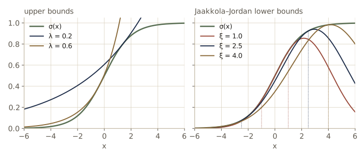
Using a bound inside an integral
Why a Gaussian-shaped bound? Bayesian predictions for classifiers need integrals like \(I = \int \sigma(a)\, \mathcal{N}(a \mid \mu, s^2)\, \mathrm{d}a\), which have no closed form. Replace \(\sigma(a)\) by its lower bound \(f(a, \xi)\): the integrand becomes the exponential of a quadratic times a Gaussian, which integrates in closed form to some \(F(\xi) \le I\). Then pick \(\xi\) to maximize \(F(\xi)\), the tightest bound in the family. The result is not exact. The bound is tight only at \(a = \pm\xi\), and the optimal \(\xi\) is a compromise over the values of \(a\) weighted by the Gaussian. The next section uses this idea on a whole likelihood.
Variational logistic regression
In module 04 we approximated the posterior of Bayesian logistic regression with the Laplace approximation. Here we use the sigmoid bound instead. It also leads to a Gaussian posterior, but through a well-defined objective: a lower bound on the evidence.
The variational posterior
The targets are \(t_n \in \{0, 1\}\) and \(a = \mathbf{w}^{\mathrm{T}} \boldsymbol{\phi}\). A convenient way to write one observation’s likelihood is
\[p(t \mid \mathbf{w}) = \sigma(a)^t (1 - \sigma(a))^{1 - t} = e^{a t} \frac{e^{-a}}{1 + e^{-a}} = e^{a t} \sigma(-a).\]Apply the lower bound to \(\sigma(-a)\) with a separate variational parameter \(\xi_n\) for each data point (the bound is even in \(\xi\), so we take \(\xi_n \ge 0\)):
\[p(t_n \mid \mathbf{w}) \ge e^{a_n t_n} \sigma(\xi_n) \exp\!\left\{ -\frac{a_n + \xi_n}{2} - \lambda(\xi_n) (a_n^2 - \xi_n^2) \right\}, \qquad a_n = \mathbf{w}^{\mathrm{T}} \boldsymbol{\phi}_n .\]Multiply over the data and by a Gaussian prior \(p(\mathbf{w}) = \mathcal{N}(\mathbf{w} \mid \mathbf{m}_0, \mathbf{S}_0)\). Call the product of the per-point bounds \(h(\mathbf{w}, \boldsymbol{\xi})\); then \(p(\mathbf{t}, \mathbf{w}) \ge h(\mathbf{w}, \boldsymbol{\xi})\, p(\mathbf{w})\). As a function of \(\mathbf{w}\) the log of the right side is
\[-\frac{1}{2} (\mathbf{w} - \mathbf{m}_0)^{\mathrm{T}} \mathbf{S}_0^{-1} (\mathbf{w} - \mathbf{m}_0) + \sum_{n=1}^{N} \left\{ (t_n - \tfrac{1}{2}) \mathbf{w}^{\mathrm{T}} \boldsymbol{\phi}_n - \lambda(\xi_n) \mathbf{w}^{\mathrm{T}} \boldsymbol{\phi}_n \boldsymbol{\phi}_n^{\mathrm{T}} \mathbf{w} \right\} + \text{const},\]a quadratic. Normalizing it gives a Gaussian \(q(\mathbf{w}) = \mathcal{N}(\mathbf{w} \mid \mathbf{m}_N, \mathbf{S}_N)\) with
\[\mathbf{S}_N^{-1} = \mathbf{S}_0^{-1} + 2 \sum_{n=1}^{N} \lambda(\xi_n) \boldsymbol{\phi}_n \boldsymbol{\phi}_n^{\mathrm{T}}, \qquad \mathbf{m}_N = \mathbf{S}_N \left( \mathbf{S}_0^{-1} \mathbf{m}_0 + \sum_{n=1}^{N} (t_n - \tfrac{1}{2}) \boldsymbol{\phi}_n \right).\]Compare the Laplace approximation, whose precision is \(\mathbf{S}_0^{-1} + \sum_n y_n (1 - y_n) \boldsymbol{\phi}_n \boldsymbol{\phi}_n^{\mathrm{T}}\) at the mode. Both are Gaussian; they differ in the weight each data point gets, \(2\lambda(\xi_n)\) against \(y_n(1 - y_n)\).
Optimizing the variational parameters
The \(\xi_n\) should make the bound on the evidence as tight as possible:
\[\ln p(\mathbf{t}) = \ln \int p(\mathbf{t} \mid \mathbf{w})\, p(\mathbf{w})\, \mathrm{d}\mathbf{w} \ge \ln \int h(\mathbf{w}, \boldsymbol{\xi})\, p(\mathbf{w})\, \mathrm{d}\mathbf{w} = \mathcal{L}(\boldsymbol{\xi}).\]One way to maximize it is EM, with \(\mathbf{w}\) playing the latent variable. The E step computes \(q(\mathbf{w})\) from the current \(\boldsymbol{\xi}\), which we just did. The M step maximizes \(\mathbb{E}_{q}[\ln h(\mathbf{w}, \boldsymbol{\xi})]\) over \(\boldsymbol{\xi}\); dropping terms free of \(\boldsymbol{\xi}\), that is
\[Q(\boldsymbol{\xi}) = \sum_{n=1}^{N} \left\{ \ln \sigma(\xi_n) - \frac{\xi_n}{2} - \lambda(\xi_n) \left( \boldsymbol{\phi}_n^{\mathrm{T}} \mathbb{E}[\mathbf{w} \mathbf{w}^{\mathrm{T}}] \boldsymbol{\phi}_n - \xi_n^2 \right) \right\}.\]Differentiate with respect to \(\xi_n\). The derivative of \(\ln \sigma(\xi) - \xi/2\) is \(\sigma(-\xi) - \tfrac{1}{2} = \tfrac{1}{2} - \sigma(\xi) = -2\xi \lambda(\xi)\), which cancels the \(+2\xi\lambda(\xi)\) from differentiating \(\lambda(\xi) \xi^2\). What is left is \(-\lambda'(\xi_n) (\boldsymbol{\phi}_n^{\mathrm{T}} \mathbb{E}[\mathbf{w} \mathbf{w}^{\mathrm{T}}] \boldsymbol{\phi}_n - \xi_n^2) = 0\). Since \(\lambda\) is strictly decreasing for \(\xi > 0\), \(\lambda' \neq 0\), and
\[\xi_n^2 = \boldsymbol{\phi}_n^{\mathrm{T}} \left( \mathbf{S}_N + \mathbf{m}_N \mathbf{m}_N^{\mathrm{T}} \right) \boldsymbol{\phi}_n .\]Each \(\xi_n\) becomes the root mean square of \(a_n\) under \(q\), so the bound is tight where \(a_n\) is likely to be. The bound itself can be evaluated in closed form, because \(h(\mathbf{w}, \boldsymbol{\xi})\, p(\mathbf{w})\) is the exponential of a quadratic in \(\mathbf{w}\). Collecting the constant terms of the log (those free of \(\mathbf{w}\)), completing the square, and using the Gaussian integral
\[\int \exp\!\left(-\tfrac{1}{2} \mathbf{w}^{\mathrm{T}} \mathbf{A} \mathbf{w} + \mathbf{b}^{\mathrm{T}} \mathbf{w}\right) \mathrm{d}\mathbf{w} = (2\pi)^{M/2} \det(\mathbf{A})^{-1/2} \exp\!\left(\tfrac{1}{2} \mathbf{b}^{\mathrm{T}} \mathbf{A}^{-1} \mathbf{b}\right)\]with \(\mathbf{A} = \mathbf{S}_N^{-1}\) and \(\mathbf{b} = \mathbf{S}_N^{-1} \mathbf{m}_N\) gives
\[\begin{aligned} \mathcal{L}(\boldsymbol{\xi}) &= \frac{1}{2} \ln \frac{\det \mathbf{S}_N}{\det \mathbf{S}_0} + \frac{1}{2} \mathbf{m}_N^{\mathrm{T}} \mathbf{S}_N^{-1} \mathbf{m}_N - \frac{1}{2} \mathbf{m}_0^{\mathrm{T}} \mathbf{S}_0^{-1} \mathbf{m}_0 \\ &\quad + \sum_{n=1}^{N} \left\{ \ln \sigma(\xi_n) - \frac{\xi_n}{2} + \lambda(\xi_n) \xi_n^2 \right\}. \end{aligned}\]Watch out. The signs of the two quadratic terms in \(\mathcal{L}(\boldsymbol{\xi})\) are easy to get backwards; the \(\mathbf{m}_N\) term comes in with a plus because it is the completed square, and the \(\mathbf{m}_0\) term with a minus from the prior’s normalizer. With the signs swapped, the “bound” goes down during the updates, and it can exceed the true log evidence. Both are quick tests worth running.
Maximizing \(\mathcal{L}(\boldsymbol{\xi})\) directly by differentiation gives the same update for \(\xi_n\) (exercise 14).
Now an experiment where we can check everything. With only two weights, the exact posterior can be computed on a fine grid over \(\mathbf{w}\), so we take a two-dimensional input and no bias term (\(\boldsymbol{\phi}(\mathbf{x}) = \mathbf{x}\)), with two overlapping classes symmetric about the origin, 30 points, and prior \(\mathcal{N}(\mathbf{0}, \alpha^{-1} \mathbf{I})\) with \(\alpha = 0.5\).
rng = np.random.default_rng(64)
N_c, alpha_c = 30, 0.5
t_c = (rng.random(N_c) < 0.5).astype(float)
centers = np.where(t_c[:, None] == 1, 1.0, -1.0) * np.array([0.9, 0.6])
X_c = rng.normal(size=(N_c, 2)) * 0.9 + centers
M_c = X_c.shape[1]
m0_c, S0inv_c = np.zeros(M_c), alpha_c * np.eye(M_c)

def vb_logistic(Phi, t, m0, S0inv, iters=50, trace=()):
    """Jaakkola-Jordan variational logistic regression by EM over xi."""
    xi = np.ones(len(t))
    bounds = []
    for it in range(iters):
        SN = np.linalg.inv(S0inv + 2 * (lam_xi(xi)[:, None] * Phi).T @ Phi)  # E step
        mN = SN @ (S0inv @ m0 + Phi.T @ (t - 0.5))
        L = (0.5 * (np.linalg.slogdet(SN)[1] + np.linalg.slogdet(S0inv)[1])
             + 0.5 * mN @ np.linalg.solve(SN, mN) - 0.5 * m0 @ S0inv @ m0
             + np.sum(np.log(expit(xi)) - xi / 2 + lam_xi(xi) * xi ** 2))
        bounds.append(L)
        if it in trace:
            print(f"iter {it:2d}: L(xi) = {L:.5f}, m_N = {mN}")
        E_wwT = SN + np.outer(mN, mN)
        xi = np.sqrt(np.einsum('ni,ij,nj->n', Phi, E_wwT, Phi))            # M step
    return mN, SN, xi, np.array(bounds)

mN_vb, SN_vb, xi_c, bounds_c = vb_logistic(X_c, t_c, m0_c, S0inv_c,
                                           trace=(0, 1, 2, 5, 10, 49))
print("bound never decreased:", bool(np.all(np.diff(bounds_c) > -1e-10)))
iter  0: L(xi) = -15.67047, m_N = [0.8838 0.6628]
iter  1: L(xi) = -12.79765, m_N = [1.2948 0.9687]
iter  2: L(xi) = -11.61084, m_N = [1.589 1.189]
iter  5: L(xi) = -10.64448, m_N = [2.0757 1.5484]
iter 10: L(xi) = -10.50253, m_N = [2.3228 1.728 ]
iter 49: L(xi) = -10.49667, m_N = [2.3864 1.7739]
bound never decreased: True
For the comparison we need the Laplace approximation from module 04 (Newton’s method to the mode, then the Hessian) and the exact posterior on a 401-by-401 grid around it. For predictions we integrate \(\sigma(a)\) against each approximation’s Gaussian over \(a\) numerically, with Gauss–Hermite quadrature, rather than with the probit approximation of module 04, so that the differences we see come from the posteriors alone.
def laplace_logistic(Phi, t, alpha, iters=30):
    w = np.zeros(Phi.shape[1])
    for _ in range(iters):
        y = expit(Phi @ w)
        H = alpha * np.eye(len(w)) + (y * (1 - y) * Phi.T) @ Phi
        w = w - np.linalg.solve(H, Phi.T @ (y - t) + alpha * w)    # Newton step
    y = expit(Phi @ w)
    H = alpha * np.eye(len(w)) + (y * (1 - y) * Phi.T) @ Phi
    # Laplace estimate of ln p(t)
    ln_ev = (np.sum(t * np.log(y) + (1 - t) * np.log(1 - y)) - 0.5 * alpha * w @ w
             + 0.5 * len(w) * np.log(alpha) - 0.5 * np.linalg.slogdet(H)[1])
    return w, np.linalg.inv(H), ln_ev

w_lap, S_lap, ln_ev_lap = laplace_logistic(X_c, t_c, alpha_c)

# exact posterior on a grid, 7 Laplace standard deviations each way
sd = np.sqrt(np.diag(S_lap))
g1 = np.linspace(w_lap[0] - 7 * sd[0], w_lap[0] + 7 * sd[0], 401)
g2 = np.linspace(w_lap[1] - 7 * sd[1], w_lap[1] + 7 * sd[1], 401)
Wg = np.stack(np.meshgrid(g1, g2, indexing='ij'), axis=-1).reshape(-1, 2)
A_g = Wg @ X_c.T
ln_lik = -(t_c * np.logaddexp(0, -A_g) + (1 - t_c) * np.logaddexp(0, A_g)).sum(axis=1)
ln_prior = -0.5 * alpha_c * (Wg ** 2).sum(axis=1) + np.log(alpha_c / (2 * np.pi))
ln_joint = ln_lik + ln_prior
ln_ev_exact = logsumexp(ln_joint) + np.log((g1[1] - g1[0]) * (g2[1] - g2[0]))
P_g = np.exp(ln_joint - logsumexp(ln_joint))
m_ex = P_g @ Wg
S_ex = (Wg - m_ex).T @ ((Wg - m_ex) * P_g[:, None])

gh_z, gh_wt = np.polynomial.hermite_e.hermegauss(40)
gh_wt = gh_wt / gh_wt.sum()
def predictive(m, S, x):
    """E[sigma(w^T x)] for w ~ N(m, S), by Gauss-Hermite quadrature over a = w^T x."""
    return np.sum(gh_wt * expit(x @ m + np.sqrt(x @ S @ x) * gh_z))

print("            mean              sd               corr     ln p(t)")
for name, m_, S_, ev in [("exact", m_ex, S_ex, ln_ev_exact),
                         ("VB", mN_vb, SN_vb, bounds_c[-1]),
                         ("Laplace", w_lap, S_lap, ln_ev_lap)]:
    s_ = np.sqrt(np.diag(S_))
    print(f"{name:8s} {m_}  {s_}  {S_[0, 1] / (s_[0] * s_[1]):6.3f}   {ev:8.4f}")
print("\n  x              exact    VB     Laplace")
for x in np.array([[0.5, 0.2], [1.0, 1.0], [2.0, -2.0], [4.0, -3.0], [-3.0, 3.5]]):
    p_ex = P_g @ expit(Wg @ x)
    p_vb, p_lap = predictive(mN_vb, SN_vb, x), predictive(w_lap, S_lap, x)
    print(f"{x}   {p_ex:.3f}   {p_vb:.3f}   {p_lap:.3f}")
            mean              sd               corr     ln p(t)
exact    [2.462  1.8307]  [0.7836 0.7112]   0.278    -9.6535
VB       [2.3864 1.7739]  [0.4746 0.4865]  -0.119   -10.4967
Laplace  [2.2774 1.6988]  [0.7772 0.6976]   0.295    -9.6613

  x              exact    VB     Laplace
[0.5 0.2]   0.823   0.822   0.805
[1. 1.]   0.976   0.981   0.966
[ 2. -2.]   0.693   0.709   0.682
[ 4. -3.]   0.882   0.914   0.864
[-3.   3.5]   0.388   0.372   0.395
The results are instructive, and not entirely in the variational method’s favor.
- The variational mean is closer to the exact posterior mean than the Laplace mean is. The Laplace approximation is centered at the mode, and this posterior is skewed, with more mass toward larger weights, so its mean lies beyond the mode.
- The variational posterior is too narrow: its standard deviations are well under the exact ones, and the correlation even has the wrong sign. The reason is visible in the precision formula. A point far from the boundary, with \(\lvert a_n \rvert\) around 3, gets weight \(y_n(1 - y_n) \approx 0.05\) in the Laplace precision but \(2\lambda(\xi_n) \approx 0.15\) in the variational one; the sigmoid bound is loose far from \(\pm\xi\), and every well-classified point adds too much certainty. The Laplace covariance, by luck of this example, is close to the exact one.
- The variational \(\ln p(\mathbf{t})\) is a true lower bound and sits below the exact value, as it must. The Laplace estimate happens to be closer here, but it carries no guarantee in either direction.
- For predictions, the over-confidence shows: away from the data, where the posterior spread matters, the variational probabilities are pushed further from 0.5 than the exact ones.
So the variational treatment buys a principled objective and a mean that accounts for skew, and pays with over-confident variances. Which matters more depends on the use. Bishop’s Figure 10.13 shows the variational predictive distribution on a separable data set.
In practice. The bound on one sigmoid applies only to two classes; it does not extend to the softmax. The Jaakkola–Jordan method is also naturally sequential: start from the prior, and for each arriving point apply the bound to its likelihood term, normalize to get a new Gaussian, and discard the point (exercise 15).
Inference of hyperparameters
So far \(\alpha\) was fixed. To infer it, give it a gamma hyperprior \(p(\alpha) = \operatorname{Gam}(\alpha \mid a_0, b_0)\) and combine both kinds of variational approximation in one model. The global decomposition gives \(\ln p(\mathbf{t}) \ge \mathcal{L}(q)\) for any \(q(\mathbf{w}, \alpha)\); the local bound, \(p(\mathbf{t} \mid \mathbf{w}) \ge h(\mathbf{w}, \boldsymbol{\xi})\), then lower-bounds \(\mathcal{L}(q)\) itself by a tractable \(\tilde{\mathcal{L}}(q, \boldsymbol{\xi})\). With \(q(\mathbf{w}, \alpha) = q(\mathbf{w})\, q(\alpha)\) the general result gives, as in the linear regression section,
\[\begin{aligned} q(\mathbf{w}) &= \mathcal{N}(\mathbf{w} \mid \boldsymbol{\mu}_N, \boldsymbol{\Sigma}_N), \\ \boldsymbol{\Sigma}_N^{-1} &= \mathbb{E}[\alpha] \mathbf{I} + 2 \sum_n \lambda(\xi_n) \boldsymbol{\phi}_n \boldsymbol{\phi}_n^{\mathrm{T}}, \qquad \boldsymbol{\Sigma}_N^{-1} \boldsymbol{\mu}_N = \sum_n (t_n - \tfrac{1}{2}) \boldsymbol{\phi}_n, \end{aligned}\] \[q(\alpha) = \operatorname{Gam}(\alpha \mid a_N, b_N), \quad a_N = a_0 + \frac{M}{2}, \quad b_N = b_0 + \frac{1}{2} \left( \boldsymbol{\mu}_N^{\mathrm{T}} \boldsymbol{\mu}_N + \operatorname{tr}(\boldsymbol{\Sigma}_N) \right),\]and the \(\xi_n\) update is unchanged, with \(\boldsymbol{\Sigma}_N + \boldsymbol{\mu}_N \boldsymbol{\mu}_N^{\mathrm{T}}\) in place of \(\mathbf{S}_N + \mathbf{m}_N \mathbf{m}_N^{\mathrm{T}}\). We cycle through the three updates.
def vb_logistic_ard(Phi, t, a0=1e-2, b0=1e-2, iters=200):
    N, M = Phi.shape
    xi, E_alpha = np.ones(N), 1.0
    aN = a0 + M / 2
    for _ in range(iters):
        prec = E_alpha * np.eye(M) + 2 * (lam_xi(xi)[:, None] * Phi).T @ Phi
        Sigma = np.linalg.inv(prec)
        mu = Sigma @ (Phi.T @ (t - 0.5))
        bN = b0 + 0.5 * (mu @ mu + np.trace(Sigma))
        E_alpha = aN / bN
        xi = np.sqrt(np.einsum('ni,ij,nj->n', Phi, Sigma + np.outer(mu, mu), Phi))
    return mu, Sigma, aN, bN

mu_h, Sigma_h, aN_h, bN_h = vb_logistic_ard(X_c, t_c)
print(f"E[alpha] = {aN_h / bN_h:.4f} (sd {np.sqrt(aN_h) / bN_h:.4f})")
print(f"mean of w: {mu_h}")
E[alpha] = 0.0535 (sd 0.0533)
mean of w: [4.9372 3.5391]
The data prefer a smaller prior precision than the 0.5 we fixed before, and the weights grow accordingly; the posterior over \(\alpha\) is broad, as it must be when only two weights inform it.
Expectation propagation
The variational methods so far all minimize \(\mathrm{KL}(q \Vert p)\). Expectation propagation (EP) is a deterministic method built on the other divergence, \(\mathrm{KL}(p \Vert q)\), which as we saw spreads \(q\) over the whole posterior instead of shrinking it inside.
Moment matching
First, what minimizes \(\mathrm{KL}(p \Vert q)\) when \(q\) is in the exponential family, \(q(\mathbf{z}) = h(\mathbf{z})\, g(\boldsymbol{\eta}) \exp\{\boldsymbol{\eta}^{\mathrm{T}} \mathbf{u}(\mathbf{z})\}\)? As a function of the natural parameters,
\[\mathrm{KL}(p \Vert q) = -\ln g(\boldsymbol{\eta}) - \boldsymbol{\eta}^{\mathrm{T}} \mathbb{E}_{p}[\mathbf{u}(\mathbf{z})] + \text{const}.\]Setting the gradient to zero gives \(-\nabla \ln g(\boldsymbol{\eta}) = \mathbb{E}_p[\mathbf{u}(\mathbf{z})]\). But differentiating the normalization condition of the exponential family (module 02) shows that \(-\nabla \ln g(\boldsymbol{\eta}) = \mathbb{E}_q[\mathbf{u}(\mathbf{z})]\). Hence
\[\mathbb{E}_{q}[\mathbf{u}(\mathbf{z})] = \mathbb{E}_{p}[\mathbf{u}(\mathbf{z})].\]The best \(q\) matches the expected sufficient statistics of \(p\). For a Gaussian \(q\), that means matching the mean and the covariance, which is moment matching; it is what we did for the two-mode density earlier.
We usually cannot compute moments of the exact posterior, so we cannot apply this directly. EP applies it one factor at a time, in a context where the moments are computable.
The algorithm
Many models have a joint distribution that is a product of factors,
\[p(\mathcal{D}, \boldsymbol{\theta}) = \prod_i f_i(\boldsymbol{\theta}),\]for example one factor \(f_n(\boldsymbol{\theta}) = p(\mathbf{x}_n \mid \boldsymbol{\theta})\) per data point and \(f_0(\boldsymbol{\theta}) = p(\boldsymbol{\theta})\) for the prior. The posterior is \(p(\boldsymbol{\theta} \mid \mathcal{D}) = \prod_i f_i(\boldsymbol{\theta}) / p(\mathcal{D})\) and the evidence is \(p(\mathcal{D}) = \int \prod_i f_i(\boldsymbol{\theta})\, \mathrm{d}\boldsymbol{\theta}\). EP approximates each factor by a simpler site function \(\tilde{f}_i(\boldsymbol{\theta})\) from the exponential family (an unnormalized Gaussian, say), so that
\[q(\boldsymbol{\theta}) = \frac{1}{Z} \prod_i \tilde{f}_i(\boldsymbol{\theta})\]is in the family too. Approximating each factor on its own, as if the others did not exist, would waste effort on regions the posterior never visits. EP instead refines one site at a time in the context of all the others:
- Initialize all sites (often to 1, with the prior site equal to the prior) and set \(q \propto \prod_i \tilde{f}_i\).
- Repeat until the sites stop changing; for each \(j\):
- Remove site \(j\) to form the cavity distribution \(q^{\setminus j}(\boldsymbol{\theta}) \propto q(\boldsymbol{\theta}) / \tilde{f}_j(\boldsymbol{\theta})\). For Gaussians, dividing means subtracting natural parameters.
- Include the exact factor: form the tilted distribution \(\hat{p}(\boldsymbol{\theta}) = f_j(\boldsymbol{\theta})\, q^{\setminus j}(\boldsymbol{\theta}) / Z_j\) with \(Z_j = \int f_j(\boldsymbol{\theta})\, q^{\setminus j}(\boldsymbol{\theta})\, \mathrm{d}\boldsymbol{\theta}\).
- Project: set \(q^{\text{new}}\) to the member of the family with the same moments as \(\hat{p}\), which minimizes \(\mathrm{KL}(\hat{p} \Vert q^{\text{new}})\).
- Update the site: \(\tilde{f}_j(\boldsymbol{\theta}) = Z_j\, q^{\text{new}}(\boldsymbol{\theta}) / q^{\setminus j}(\boldsymbol{\theta})\). The factor \(Z_j\) makes the site integrate against the cavity to the same value as the exact factor does.
- Approximate the evidence by \(p(\mathcal{D}) \approx \int \prod_i \tilde{f}_i(\boldsymbol{\theta})\, \mathrm{d}\boldsymbol{\theta}\).
The moments of the tilted distribution are computable because it involves only one exact factor times a Gaussian, a low-dimensional or otherwise easy integral. The cavity focuses the approximation of \(f_j\) on the region where the rest of the posterior puts its mass.
A one-pass version, which initializes every site except the prior to 1 and updates each site once in order, is called assumed density filtering (ADF). It suits streaming data, but its answer depends on the order of the data. EP revisits every site until the whole set is consistent, which removes the order dependence.
Watch out. EP has no guarantee of convergence, and a single update need not improve any objective. When it converges, the result is a stationary point of a certain energy function, but EP does not climb a bound the way variational Bayes does. In practice, damping the site updates and skipping updates whose cavity would have negative variance make it reliable on most problems. And since it minimizes \(\mathrm{KL}(p \Vert q)\), EP is a poor choice for multimodal posteriors such as mixtures, where it averages over modes; it shines on unimodal ones, such as those of logistic-type models.
Example: the clutter problem
We want the mean \(\theta\) of a Gaussian observation model, but each observation is, with known probability \(w\), replaced by clutter from a broad background Gaussian:
\[p(x \mid \theta) = (1 - w)\, \mathcal{N}(x \mid \theta, 1) + w\, \mathcal{N}(x \mid 0, a), \qquad p(\theta) = \mathcal{N}(\theta \mid 0, b).\]We work in one dimension and use \(w = 0.5\), \(a = 10\), \(b = 100\). The likelihood of \(N\) points is a product of \(N\) two-term sums, so the exact posterior is a mixture of \(2^N\) Gaussians, out of reach for large \(N\). In one dimension, though, we can compute it on a fine grid, which gives us the exact answer to compare with.
EP uses a Gaussian \(q(\theta)\) and Gaussian-shaped sites \(\tilde{f}_n(\theta) \propto \exp(-\frac{1}{2} \tau_n \theta^2 + \nu_n \theta)\). We store each site by its natural parameters, precision \(\tau_n\) and precision-times-mean \(\nu_n\), so that multiplying and dividing Gaussians is adding and subtracting. A site is not a density: its precision can be zero (the initial site, a constant) or even negative (a site that curves upward), and only \(q\) itself needs a positive precision. The prior is its own exact site, \(\tau_0 = 1/b\), \(\nu_0 = 0\), and never needs updating.
For site \(n\), the cavity has precision \(\tau - \tau_n\) and \(\nu - \nu_n\); write its mean and variance as \(m^{\setminus n}\) and \(v^{\setminus n}\). The tilted distribution is the cavity times a two-component mixture, and its normalizer and moments come from the Gaussian integrals of module 02 (exercise 16):
\[\begin{aligned} Z_n &= (1 - w)\, \mathcal{N}(x_n \mid m^{\setminus n}, v^{\setminus n} + 1) + w\, \mathcal{N}(x_n \mid 0, a), \\ \rho_n &= \frac{(1 - w)\, \mathcal{N}(x_n \mid m^{\setminus n}, v^{\setminus n} + 1)}{Z_n}, \\ m^{\text{new}} &= m^{\setminus n} + \rho_n \frac{v^{\setminus n}}{v^{\setminus n} + 1} (x_n - m^{\setminus n}), \\ v^{\text{new}} &= v^{\setminus n} - \rho_n \frac{(v^{\setminus n})^2}{v^{\setminus n} + 1} + \rho_n (1 - \rho_n) \frac{(v^{\setminus n})^2 (x_n - m^{\setminus n})^2}{(v^{\setminus n} + 1)^2}. \end{aligned}\]Here \(\rho_n\) is the posterior probability, under the cavity, that \(x_n\) is a real observation rather than clutter. The new site is the new \(q\) divided by the cavity: \(\tau_n = 1/v^{\text{new}} - (\tau - \tau_n)\) and similarly for \(\nu_n\).
For the evidence we need the scale of each site. Write \(A(\tau, \nu) = \frac{1}{2} \ln(2\pi / \tau) + \nu^2 / (2\tau)\) for the log of \(\int \exp(-\frac{1}{2}\tau\theta^2 + \nu\theta)\, \mathrm{d}\theta\). Then a normalized Gaussian with natural parameters \((\tau, \nu)\) is \(\exp(-\frac{1}{2}\tau\theta^2 + \nu\theta - A(\tau, \nu))\), and the site \(\tilde{f}_n = Z_n q / q^{\setminus n}\) carries the constant \(\ln Z_n - A(q) + A(q^{\setminus n})\). Multiplying the prior and all sites and integrating gives
\[\ln p(\mathcal{D}) \approx A(\tau, \nu) - A(\tau_0, \nu_0) + \sum_{n=1}^{N} \left\{ \ln Z_n + A(\tau - \tau_n, \nu - \nu_n) - A(\tau, \nu) \right\},\]where \((\tau, \nu)\) are the natural parameters of the final \(q\) (exercise 17). This form works even when some site precisions are negative.
def ln_normal(x, m, v):
    return -0.5 * np.log(2 * np.pi * v) - 0.5 * (x - m) ** 2 / v

def A_nat(tau, nu):
    """log of the integral of exp(-tau theta^2 / 2 + nu theta)."""
    return 0.5 * np.log(2 * np.pi / tau) + 0.5 * nu ** 2 / tau

def ep_clutter(x, w, a, b, max_passes=50, tol=1e-9, trace=False):
    """EP for the 1-D clutter problem.
    Returns mean and variance of q, ln evidence, site precisions, ADF result."""
    N = len(x)
    tau_s, nu_s, lnZ_s = np.zeros(N), np.zeros(N), np.zeros(N)
    tau, nu = 1 / b, 0.0                                  # q starts at the prior
    for p in range(max_passes):
        old = np.r_[tau_s, nu_s]
        for n in range(N):
            tau_c, nu_c = tau - tau_s[n], nu - nu_s[n]    # cavity (remove site n)
            if tau_c <= 0:
                continue                 # skip: the cavity is not a proper Gaussian
            v_c, m_c = 1 / tau_c, nu_c / tau_c
            ln_real = np.log(1 - w) + ln_normal(x[n], m_c, v_c + 1)
            ln_clut = np.log(w) + ln_normal(x[n], 0.0, a)
            lnZ = np.logaddexp(ln_real, ln_clut)     # normalizer of tilted distribution
            rho = np.exp(ln_real - lnZ)
            m_new = m_c + rho * v_c / (v_c + 1) * (x[n] - m_c)
            v_new = (v_c - rho * v_c ** 2 / (v_c + 1)
                     + rho * (1 - rho) * (v_c * (x[n] - m_c) / (v_c + 1)) ** 2)
            tau, nu = 1 / v_new, m_new / v_new            # projected q
            tau_s[n], nu_s[n] = tau - tau_c, nu - nu_c     # new site = q / cavity
            lnZ_s[n] = lnZ
        ln_ev = A_nat(tau, nu) - A_nat(1 / b, 0.0) + np.sum(
            lnZ_s + A_nat(tau - tau_s, nu - nu_s) - A_nat(tau, nu))
        change = np.abs(np.r_[tau_s, nu_s] - old).max()
        if p == 0:
            adf = (nu / tau, 1 / tau, lnZ_s.sum())   # one pass = ADF
        if trace:
            print(f"pass {p + 1}: mean {nu / tau:.6f}, var {1 / tau:.6f}, "
                  f"ln p(D) {ln_ev:.5f}, site change {change:.1e}")
        if change < tol:
            break
    return nu / tau, 1 / tau, ln_ev, tau_s, adf
In the ADF pass, each site is computed with the approximation built from the points before it as its cavity, so the product of the \(Z_n\) from that pass is ADF’s own estimate of the evidence; that is what the function records. Now some data: 25 points, about half of them clutter, with true \(\theta = 2\).
w_cl, a_cl, b_cl = 0.5, 10.0, 100.0
rng = np.random.default_rng(2)
N_cl, theta_true = 25, 2.0
is_clutter = rng.random(N_cl) < w_cl
x_cl = np.where(is_clutter, rng.normal(0, np.sqrt(a_cl), N_cl),
                rng.normal(theta_true, 1.0, N_cl))
print(f"{is_clutter.sum()} of {N_cl} points are clutter; mean of all {x_cl.mean():.3f}")

m_ep, v_ep, ln_ev_ep, tau_sites, adf = ep_clutter(x_cl, w_cl, a_cl, b_cl, trace=True)
print(f"{np.sum(tau_sites < 0)} of {N_cl} site precisions are negative")
13 of 25 points are clutter; mean of all 1.266
pass 1: mean 2.007417, var 0.249579, ln p(D) -60.51438, site change 1.5e+00
pass 2: mean 2.192650, var 0.126650, ln p(D) -57.42706, site change 1.7e+00
pass 3: mean 2.192169, var 0.126391, ln p(D) -57.32841, site change 1.8e-01
pass 4: mean 2.192135, var 0.126463, ln p(D) -57.33222, site change 2.1e-03
pass 5: mean 2.192135, var 0.126465, ln p(D) -57.33236, site change 6.1e-05
pass 6: mean 2.192135, var 0.126465, ln p(D) -57.33236, site change 1.4e-06
pass 7: mean 2.192135, var 0.126465, ln p(D) -57.33236, site change 3.2e-08
pass 8: mean 2.192135, var 0.126465, ln p(D) -57.33236, site change 1.4e-09
pass 9: mean 2.192135, var 0.126465, ln p(D) -57.33236, site change 2.6e-11
9 of 25 site precisions are negative
EP settles to six digits within five passes, and the site change keeps shrinking by one to two orders of magnitude per pass after that. The exact posterior on a grid, for comparison:
theta = np.linspace(-10, 15, 50001); dth = theta[1] - theta[0]
ln_post = ln_normal(theta, 0.0, b_cl) + np.logaddexp(
    np.log(1 - w_cl) + ln_normal(x_cl[:, None], theta, 1.0),
    np.log(w_cl) + ln_normal(x_cl[:, None], 0.0, a_cl)).sum(axis=0)
ln_ev_cl = logsumexp(ln_post) + np.log(dth)
P_th = np.exp(ln_post - logsumexp(ln_post))
m_cl = P_th @ theta
v_cl = P_th @ (theta - m_cl) ** 2
print("          mean       var        ln p(D)")
print(f"exact   {m_cl:.5f}   {v_cl:.5f}   {ln_ev_cl:.4f}")
print(f"EP      {m_ep:.5f}   {v_ep:.5f}   {ln_ev_ep:.4f}")
print(f"ADF     {adf[0]:.5f}   {adf[1]:.5f}   {adf[2]:.4f}")
          mean       var        ln p(D)
exact   2.19188   0.12637   -57.3328
EP      2.19214   0.12647   -57.3324
ADF     2.00742   0.24958   -58.4375
EP matches the exact posterior mean to about three decimal places, the variance to about three significant digits, and the log evidence to a small fraction of a nat. One pass of ADF is much worse on all three, because the early sites were fitted with cavities that knew almost nothing about \(\theta\); the extra passes of EP go back and refit those sites once the rest of the posterior has sharpened.
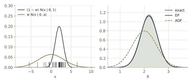
On this problem Bishop §10.7.1 compares EP with variational Bayes and the Laplace approximation as a function of computing time; EP is the most accurate of the three, at a higher cost per unit of accuracy early on.
Expectation propagation on graphs
So far each site \(\tilde{f}_i\) was a function of all of \(\boldsymbol{\theta}\). On a graphical model, each factor \(f_j(\boldsymbol{\theta}_j)\) depends only on a subset \(\boldsymbol{\theta}_j\) of the variables. Choose the most restrictive approximating family: \(q\) fully factorized over variables, and each site a product of one function per variable in its factor, \(\tilde{f}_j(\boldsymbol{\theta}_j) = \prod_{l} \tilde{f}_{jl}(\theta_l)\).
Now run EP. Removing site \(j\) and multiplying in the exact factor \(f_j\) gives a tilted distribution; projecting it onto a fully factorized \(q\) means taking its single-variable marginals, since \(\mathrm{KL}(p \Vert q)\) over factorized \(q\) is minimized by the marginals, as we showed early in this module. Dividing by the cavity, every piece that does not touch factor \(j\) cancels, and the new site component for variable \(\theta_l\) is
\[\tilde{f}_{jl}(\theta_l) \propto \sum_{\boldsymbol{\theta}_j \setminus \theta_l} f_j(\boldsymbol{\theta}_j) \prod_{m \neq l} \prod_{k \neq j} \tilde{f}_{km}(\theta_m),\]a sum over the other variables of factor \(j\) of the factor times the incoming site components from all other factors on those variables. That is precisely the sum-product message from factor \(j\) to variable \(\theta_l\) from module 08, with the variable-to-factor messages folded in. So belief propagation is EP with a fully factorized approximation. On a tree, with the usual two-pass schedule, it is exact; on a graph with loops, it is loopy belief propagation, which is why loopy BP can be understood as an approximate inference method. Using a less factorized \(q\) (keeping some variables together) or refining groups of factors jointly gives more accurate variants. The alpha-divergence family ties these together: variational message passing, loopy belief propagation, EP, and several newer schemes all arise as local minimizations of different members of it.
Summary
| Method | What it optimizes | Form of the approximation | Typical error |
|---|---|---|---|
| Laplace (module 04) | nothing; a local expansion at the mode | Gaussian at the mode | misses skew; no bound on the evidence |
| Mean-field variational Bayes | \(\mathcal{L}(q)\), i.e. \(\mathrm{KL}(q \Vert p)\), by coordinate ascent | product of factors, forms derived | variances too small; locks onto one mode |
| Variational mixture of Gaussians | \(\mathcal{L}(q)\) by variational E and M steps | \(q(\mathbf{Z})\, q(\boldsymbol{\pi}) \prod_k q(\boldsymbol{\mu}_k, \boldsymbol{\Lambda}_k)\) | local maxima; add \(\ln K!\) when comparing \(K\) |
| Variational linear regression | \(\mathcal{L}(q)\), alternating two updates | Gaussian \(q(\mathbf{w})\) times gamma \(q(\alpha)\) | none beyond mean field; matches the evidence approximation |
| Variational logistic regression | a bound on \(\ln p(\mathbf{t})\) from \(\sigma(a) \ge f(a, \xi)\), by EM over \(\xi_n\) | Gaussian \(q(\mathbf{w})\) | good mean; over-confident variances |
| Expectation propagation | local \(\mathrm{KL}(p \Vert q)\) by moment matching | product of exponential-family sites | may not converge; poor on multimodal posteriors |
Ideas to carry forward:
- For any \(q\), \(\ln p(\mathbf{X}) = \mathcal{L}(q) + \mathrm{KL}(q \Vert p)\). Maximizing the lower bound fits \(q\) and estimates the evidence at the same time, and monitoring the bound is the best test of an implementation.
- In a factorized family the optimal factor is \(\ln q_j^\star = \mathbb{E}_{i \neq j}[\ln p(\mathbf{X}, \mathbf{Z})] + \text{const}\). In conjugate-exponential models every factor has the prior’s form, and the updates add expected sufficient statistics to the prior’s pseudo-counts, just like an M step.
- The direction of the KL divergence decides the character of the approximation: \(\mathrm{KL}(q \Vert p)\) (variational Bayes) is compact and mode-seeking, \(\mathrm{KL}(p \Vert q)\) (EP) is broad and mass-covering.
- Bayesian treatments with variational inference choose model complexity by themselves: surplus mixture components switch off, and the bound peaks at a sensible polynomial degree or number of clusters.
Exercises
- For the factorized approximation to the correlated Gaussian, show that the coupled equations for \(m_1\) and \(m_2\) have the unique solution \(m_1 = \mu_1\), \(m_2 = \mu_2\) when \(\boldsymbol{\Lambda}\) is nonsingular. Then show that one sweep of coordinate ascent multiplies the error \(m_2 - \mu_2\) by \(\rho^2\), where \(\rho\) is the correlation coefficient, and confirm the rate in the output of the first code cell.
- Show that the alpha divergence tends to \(\mathrm{KL}(p \Vert q)\) as \(\alpha \to 1\) and to \(\mathrm{KL}(q \Vert p)\) as \(\alpha \to -1\). (Write the integrand as \(p \exp(\frac{1-\alpha}{2} \ln (q/p))\) and expand for \(\alpha\) near 1.) Then compute \(D_\alpha\) on the grid for the two-mode density of this module and find the single Gaussian that minimizes it for \(\alpha = -1, 0, 1\). How does the answer move as \(\alpha\) increases?
- Derive the lower bound for model comparison with \(q(\mathbf{Z}, m) = q(\mathbf{Z} \mid m)\, q(m)\), and show with a Lagrange multiplier that the optimal \(q(m)\) is proportional to \(p(m) \exp(\mathcal{L}_m)\). What is the value of the combined bound at that optimum?
- For the Gaussian with unknown mean and precision, first show that at convergence \(\mathbb{E}_q[\tau]\) equals the exact posterior mean \(a_N^{\text{ex}} / b_N^{\text{ex}}\) for any prior settings. (Use \(\lambda_N = (\lambda_0 + N)\mathbb{E}[\tau]\) to simplify \(b_N\).) Then take the broad-prior limit \(a_0 = b_0 = \lambda_0 = 0\) and solve the fixed-point equations in closed form. Show that \(1/\mathbb{E}[\tau] = \frac{1}{N} \sum_n (x_n - \bar{x})^2\). Now repeat with a prior on \(\mu\) that does not depend on \(\tau\) (a flat prior), and show that you get \(\frac{1}{N - 1} \sum_n (x_n - \bar{x})^2\) instead. Which term makes the difference? (Bishop’s equations (10.29)–(10.33) correspond to the second case.)
- Starting from the \((\boldsymbol{\mu}_k, \boldsymbol{\Lambda}_k)\) terms of \(\ln q^\star(\boldsymbol{\pi}, \boldsymbol{\mu}, \boldsymbol{\Lambda})\), derive the Gaussian–Wishart factor and the update equations for \(\beta_k\), \(\mathbf{m}_k\), \(\mathbf{W}_k\), and \(\nu_k\). (First collect the terms quadratic in \(\boldsymbol{\mu}_k\) to find \(q^\star(\boldsymbol{\mu}_k \mid \boldsymbol{\Lambda}_k)\), then divide it out of the joint factor to get \(q^\star(\boldsymbol{\Lambda}_k)\).)
- Verify the formula for the expected quadratic form \((\mathbf{x} - \boldsymbol{\mu}_k)^{\mathrm{T}} \boldsymbol{\Lambda}_k (\mathbf{x} - \boldsymbol{\mu}_k)\) under the Gaussian–Wishart factor. (Average over \(\boldsymbol{\mu}_k\) given \(\boldsymbol{\Lambda}_k\) first.) Then check it, and the formula for \(\mathbb{E}[\ln \det \boldsymbol{\Lambda}_k]\), by Monte Carlo: draw Wishart samples with
scipy.stats.wishart(note its scale parameter is our \(\mathbf{W}\)) and Gaussian means given each sample. - Derive two of the terms of the mixture lower bound, \(\mathbb{E}[\ln p(\mathbf{X} \mid \mathbf{Z}, \boldsymbol{\mu}, \boldsymbol{\Lambda})]\) and \(\mathbb{E}[\ln q(\boldsymbol{\pi})]\). Then test
vb_boundnumerically: perturb one entry of \(\mathbf{m}_k\) after an M step and confirm that the bound goes down, for several \(k\) and both directions. - Derive the Student’s t mixture for the predictive density of the variational mixture, including the scale matrix \(\mathbf{L}_k\). Then check
vb_predictiveagainst Monte Carlo: sample parameters from \(q\), average the mixture density at a few test points. - Show that a mixture with \(K\) components has \(K!\) equivalent parameter settings. Explain why, when the posterior modes are well separated, the variational bound underestimates the log evidence by about \(\ln K!\). Rerun the model selection experiment with \(\alpha_0 = 10^{-3}\) instead of 1: what happens to the bound for \(K > 3\), and why does adding \(\ln K!\) now mislead? How should the correction change when some components are switched off?
- Extend
vb_linregto put a gamma prior on the noise precision \(\beta\) as well, with \(q(\mathbf{w})\, q(\alpha)\, q(\beta)\). Derive the three updates, implement them, and compare \(\mathbb{E}[\beta]\) with the true value 16 on the module’s data for polynomial degrees 3 and 9. - Show directly that the fixed point of \(\alpha = M / (\mathbf{m}_N^{\mathrm{T}} \mathbf{m}_N + \operatorname{tr}\mathbf{S}_N)\) satisfies \(\alpha = \gamma / \mathbf{m}_N^{\mathrm{T}} \mathbf{m}_N\) with \(\gamma = \sum_i \lambda_i / (\alpha + \lambda_i)\), so that the two re-estimation rules have the same fixed points.
- Derive the five terms of the lower bound for variational linear regression, and verify
vb_linreg_boundby showing numerically that the bound is at most \(\ln p(\mathbf{t})\) computed by integrating over \(\alpha\) on a one-dimensional grid (for fixed \(\alpha\), \(p(\mathbf{t} \mid \alpha)\) is the evidence of module 03). - Show that \(\ln \sigma(x)\) is concave in \(x\), and that \(f(x) = -\ln(e^{x/2} + e^{-x/2})\) is convex as a function of \(y = x^2\) for \(y > 0\). Then show that \(\lambda(\xi)\) is positive and strictly decreasing for \(\xi > 0\), with \(\lambda(0) = 1/8\).
- Evaluate \(\mathcal{L}(\boldsymbol{\xi})\) for variational logistic regression by completing the square, and show that setting its derivative with respect to \(\xi_n\) to zero gives the same update as the EM argument. Then check your derivative with finite differences using the module’s code.
- Implement the sequential version of variational logistic regression: start from the prior, and for each data point in turn, update \(\mathbf{m}\) and \(\mathbf{S}\) using only that point (iterating its single \(\xi\) a few times), then move on. Compare the final Gaussian with the batch result, for two different orders of the data.
- Derive the EP update for the clutter problem: show that \(Z_n\) is as stated, and derive \(m^{\text{new}}\) and \(v^{\text{new}}\) by differentiating \(\ln Z_n\) with respect to \(m^{\setminus n}\) and \(v^{\setminus n}\). (For a Gaussian cavity, the tilted mean is \(m^{\setminus n} + v^{\setminus n}\, \partial \ln Z_n / \partial m^{\setminus n}\).)
- Derive the EP estimate of \(\ln p(\mathcal{D})\) in terms of \(A(\tau, \nu)\). Then add damping to
ep_clutter(replace each new site by a convex combination of the old and new natural parameters) and find a data set, for instance with \(w\) close to 1 or with far-away points, on which undamped EP oscillates but damped EP converges. - In your own words: explain to a classmate why variational Bayes tends to underestimate posterior variance while EP does not, using the two figures of this module that show the two KL divergences, and say which one you would use for a mixture posterior and which for a logistic regression posterior.
Going further
- Bishop, Pattern Recognition and Machine Learning, chapter 10 — the source for this module. Exercises 10.1–10.4 cover the two KL divergences, 10.7–10.9 the univariate Gaussian, 10.12–10.24 the variational mixture (10.18 derives the updates from the bound, 10.22 the \(\ln K!\) correction), 10.26–10.27 variational linear regression, 10.29–10.35 local bounds and variational logistic regression, and 10.36–10.39 expectation propagation and the clutter problem. Appendix B lists the Dirichlet, gamma, and Wishart facts used here, and Appendix D the calculus of variations.
- M. I. Jordan, Z. Ghahramani, T. S. Jaakkola, and L. K. Saul, “An introduction to variational methods for graphical models”, Machine Learning, 1999 — the classic tutorial, including convex duality and local bounds.
- D. M. Blei, A. Kucukelbir, and J. D. McAuliffe, “Variational inference: a review for statisticians”, Journal of the American Statistical Association, 2017 — a modern overview of mean-field methods and their stochastic, large-scale versions.
- M. J. Wainwright and M. I. Jordan, “Graphical models, exponential families, and variational inference”, Foundations and Trends in Machine Learning, 2008 — the general theory that connects mean field, belief propagation, and EP through the exponential family.
- T. P. Minka, A Family of Algorithms for Approximate Bayesian Inference, PhD thesis, MIT, 2001 — the thesis that introduced expectation propagation; the clutter problem is one of its examples.
- D. J. C. MacKay, Information Theory, Inference, and Learning Algorithms (Cambridge University Press, 2003), chapter 33 — a short, readable account of variational free energy minimization, including the Gaussian example of this module; the book is free to read online.
These notes follow the chapters of C. M. Bishop, Pattern Recognition and Machine Learning (Springer, 2006), the course text, which Microsoft Research makes freely available as a PDF. The explanations, code, figures, and exercises here are written for this course; the book remains the reference, with the full derivations and many more exercises.