CSE 474/574 · Module 02 · Week 2
Probability Distributions
Bernoulli, beta, multinomial, and Dirichlet; the Gaussian in depth; the exponential family and conjugate priors; kernel density and nearest-neighbor estimators.
Companion reading: Bishop, Pattern Recognition and Machine Learning, chapter 2, “Probability Distributions”
By the end of this module you can
- Fit Bernoulli and multinomial models by maximum likelihood, explain why the estimates overfit small samples, and repair them with beta and Dirichlet priors updated one observation at a time.
- Explain conjugacy, and read the parameters of a beta, Dirichlet, or gamma prior as counts of imaginary observations.
- Describe a multivariate Gaussian through the eigenvectors and eigenvalues of its covariance, compute Mahalanobis distances, and count the parameters of full, diagonal, and isotropic models.
- Derive the conditional and marginal distributions of a partitioned Gaussian by completing the square, and check them by sampling.
- Use the linear-Gaussian results to go from \(p(\mathbf{x})\) and \(p(\mathbf{y} \mid \mathbf{x})\) to \(p(\mathbf{y})\) and \(p(\mathbf{x} \mid \mathbf{y})\).
- Estimate a Gaussian’s parameters by maximum likelihood, sequentially, and in a Bayesian way with Gaussian, gamma, and normal-gamma priors, and explain why the maximum likelihood variance is biased.
- Explain Student’s t as an infinite mixture of Gaussians and why it resists outliers, average angles with the von Mises model, and write down the log-likelihood of a Gaussian mixture.
- Put a distribution in exponential-family form and find its sufficient statistics, maximum likelihood solution, and conjugate prior; estimate densities with histograms, kernels, and nearest neighbors, and implement a K-nearest-neighbor classifier.
Contents
- Binary variables
- Multinomial variables
- The Gaussian distribution
- Geometry: eigenvectors and Mahalanobis distance
- Moments
- How many parameters?
- Conditional Gaussians
- Marginal Gaussians
- Bayes’ theorem for linear-Gaussian models
- Maximum likelihood for the Gaussian
- Sequential estimation
- Bayesian inference for the Gaussian
- Student’s t-distribution
- Periodic variables
- Mixtures of Gaussians
- The exponential family
- Nonparametric methods
- Summary
- Exercises
- Going further
Module 01 set up the language of the course: probability as a way to reason about uncertainty, Bayes’ theorem, maximum likelihood, and the warning that a model with too much freedom will fit the noise in a small data set. It used one distribution, the Gaussian, almost without comment. This module slows down and studies the distributions themselves.
The task running through the module is density estimation: given observations \(x_1, \dots, x_N\), assumed independent and drawn from the same unknown distribution (i.i.d.), build a model of that distribution \(p(x)\). The task has no unique answer. Any density that is positive at the observed points could have produced them, so choosing a model is a question of model selection, the same question module 01 met with polynomial degree.
We take two routes. The first is parametric: pick a family of distributions with a few adjustable parameters (a coin’s probability of heads, a Gaussian’s mean and covariance) and fit the parameters, either by maximizing the likelihood or by putting a prior on them and computing a posterior. Along the way we meet conjugate priors, which keep the posterior in the same family as the prior and make Bayesian updating a matter of adding counts. The second route is nonparametric: histograms, kernel density estimates, and nearest neighbors, whose form is set by the data rather than fixed in advance. Every later module leans on something here, and the Gaussian results of section 3 in particular come back in modules 03, 06, 09, 12, and 13.
import numpy as np
from scipy.special import gammaln, logsumexp, expit, i0e, i1e
from scipy.linalg import solve_triangular
from scipy import stats          # used only to check our own code

np.set_printoptions(precision=4, suppress=True)
rng = np.random.default_rng(2)
Binary variables
The Bernoulli distribution and maximum likelihood
Start with the simplest random quantity there is: a variable \(x \in \{0, 1\}\), such as the result of flipping a coin that may be bent, with \(x = 1\) for heads. One number describes it, \(\mu = p(x = 1 \mid \mu)\), with \(0 \le \mu \le 1\). Both outcomes fit in one formula,
\[\operatorname{Bern}(x \mid \mu) = \mu^{x} (1 - \mu)^{1 - x},\]the Bernoulli distribution. Setting \(x = 1\) leaves \(\mu\) and setting \(x = 0\) leaves \(1 - \mu\). Its mean is \(\mathbb{E}[x] = 0 \cdot (1 - \mu) + 1 \cdot \mu = \mu\), and since \(x^2 = x\) its variance is \(\mathbb{E}[x^2] - \mu^2 = \mu(1 - \mu)\).
Suppose we flip the coin \(N\) times and record \(\mathcal{D} = \{x_1, \dots, x_N\}\). Because the flips are independent, the likelihood (the probability of the data, viewed as a function of \(\mu\)) is a product, and its logarithm is a sum:
\[\ln p(\mathcal{D} \mid \mu) = \sum_{n=1}^{N} \bigl\{ x_n \ln \mu + (1 - x_n) \ln (1 - \mu) \bigr\} = m \ln \mu + (N - m) \ln (1 - \mu),\]where \(m = \sum_n x_n\) is the number of heads. The data enter only through \(m\) (and \(N\)). A function of the data that carries everything the likelihood needs is called a sufficient statistic; we will see in section 4 that this is a general feature of a large family of distributions. Setting the derivative \(m/\mu - (N - m)/(1 - \mu)\) to zero gives the maximum likelihood (ML) estimate
\[\mu_{\mathrm{ML}} = \frac{m}{N} = \frac{1}{N} \sum_{n=1}^{N} x_n,\]the fraction of heads, also called the sample mean. We check it on simulated flips of a coin with \(\mu = 0.3\), by comparing with a brute-force search over a grid of \(\mu\) values.
def bernoulli_loglik(mu, x):
    """ln p(D | mu) for binary data x: m ln mu + (N - m) ln(1 - mu)."""
    m, N = np.sum(x), len(x)
    return m * np.log(mu) + (N - m) * np.log1p(-mu)

rng_coin = np.random.default_rng(127)
flips = (rng_coin.random(100) < 0.3).astype(int)     # 100 flips, mu = 0.3
x = flips[:20]
print("first 20 flips:", x)
print(f"m = {x.sum()} heads in N = {len(x)} flips, mu_ML = {x.mean():.3f}")
grid = np.linspace(0.001, 0.999, 999)
best = grid[np.argmax(bernoulli_loglik(grid, x))]
print(f"grid maximizer of the log-likelihood: {best:.3f}")
print(f"first 3 flips: {flips[:3]} -> mu_ML = {flips[:3].mean():.3f}")
first 20 flips: [1 1 1 0 0 0 0 0 1 1 0 1 0 0 0 0 0 0 0 0]
m = 6 heads in N = 20 flips, mu_ML = 0.300
grid maximizer of the log-likelihood: 0.300
first 3 flips: [1 1 1] -> mu_ML = 1.000
The estimate from 20 flips, 0.30, happens to be right on target. The one from the first three flips is not: all three came up heads, so maximum likelihood says \(\mu = 1\) and predicts that the coin will never show tails. This is overfitting in its most extreme form. With very little data, the maximum likelihood answer takes the sample at face value, and a run of three heads is not rare even for a coin that favors tails (it happens with probability \(0.3^3 \approx 0.03\)). A prior will fix it.
The binomial distribution
The number of heads \(m\) in \(N\) flips is itself a random variable. Each particular sequence with \(m\) heads has probability \(\mu^m (1 - \mu)^{N-m}\), and there are \(\binom{N}{m} = \frac{N!}{m!\,(N-m)!}\) such sequences, so
\[\operatorname{Bin}(m \mid N, \mu) = \binom{N}{m} \mu^{m} (1 - \mu)^{N - m}.\]This is the binomial distribution. Since \(m = x_1 + \dots + x_N\) is a sum of independent Bernoulli variables, and means and variances of independent variables add, \(\mathbb{E}[m] = N\mu\) and \(\operatorname{var}[m] = N\mu(1 - \mu)\). We compute the binomial coefficient through \(\ln \Gamma\) (for integers, \(\Gamma(n + 1) = n!\)), which avoids overflowing factorials for large \(N\).
def binom_pmf(m, N, mu):
    """Bin(m | N, mu), with the binomial coefficient computed through log-gamma."""
    log_coef = gammaln(N + 1) - gammaln(m + 1) - gammaln(N - m + 1)
    return np.exp(log_coef + m * np.log(mu) + (N - m) * np.log1p(-mu))

N, mu = 10, 0.25
m = np.arange(N + 1)
pm = binom_pmf(m, N, mu)
print(f"sum over m = {pm.sum():.6f}")
print(f"mean = {np.sum(m * pm):.4f}   (N mu = {N * mu:.4f})")
print(f"var  = {np.sum((m - N * mu)**2 * pm):.4f}   "
      f"(N mu (1 - mu) = {N * mu * (1 - mu):.4f})")
print("matches scipy.stats.binom:", np.allclose(pm, stats.binom.pmf(m, N, mu)))
sum over m = 1.000000
mean = 2.5000   (N mu = 2.5000)
var  = 1.8750   (N mu (1 - mu) = 1.8750)
matches scipy.stats.binom: True
The beta prior and conjugacy
To treat \(\mu\) in a Bayesian way we need a prior \(p(\mu)\). Any density on \([0, 1]\) would do in principle, but one choice makes the algebra collapse. The likelihood is a product of powers of \(\mu\) and \(1 - \mu\). If the prior has the same shape, the posterior, being proportional to prior times likelihood, has it too.
Definition. A prior is conjugate to a likelihood if the posterior belongs to the same family of distributions as the prior. Updating a conjugate prior only changes its parameters.
The family with the right shape is the beta distribution,
\[\operatorname{Beta}(\mu \mid a, b) = \frac{\Gamma(a + b)}{\Gamma(a)\,\Gamma(b)} \, \mu^{a - 1} (1 - \mu)^{b - 1}, \qquad a, b > 0,\]where \(\Gamma(a) = \int_0^\infty u^{a-1} e^{-u} \, du\) is the gamma function, which extends the factorial to real arguments (\(\Gamma(a + 1) = a\,\Gamma(a)\)). The ratio of gamma functions in front is exactly what makes the density integrate to one (Bishop’s exercise 2.5 proves it). The mean and variance are
\[\mathbb{E}[\mu] = \frac{a}{a + b}, \qquad \operatorname{var}[\mu] = \frac{ab}{(a + b)^2 (a + b + 1)}.\]Parameters of a prior, like \(a\) and \(b\), are called hyperparameters, to separate them from the parameter \(\mu\) they describe. With \(a = b = 1\) the beta density is uniform; larger values concentrate it. We check the normalization and the mean numerically.
def beta_logpdf(mu, a, b):
    """ln Beta(mu | a, b)."""
    return (gammaln(a + b) - gammaln(a) - gammaln(b)
            + (a - 1) * np.log(mu) + (b - 1) * np.log1p(-mu))

grid = np.linspace(0, 1, 20001)[1:-1]
for a, b in [(2, 2), (3, 7), (5, 2), (10, 20)]:
    p = np.exp(beta_logpdf(grid, a, b))
    print(f"a = {a:2d}, b = {b:2d}: area {np.trapezoid(p, grid):.4f}, "
          f"mean {np.trapezoid(grid * p, grid):.4f} (a/(a+b) = {a / (a + b):.4f})")
print("matches scipy.stats.beta:",
      np.allclose(np.exp(beta_logpdf(grid, 5, 2)), stats.beta.pdf(grid, 5, 2)))
a =  2, b =  2: area 1.0000, mean 0.5000 (a/(a+b) = 0.5000)
a =  3, b =  7: area 1.0000, mean 0.3000 (a/(a+b) = 0.3000)
a =  5, b =  2: area 1.0000, mean 0.7143 (a/(a+b) = 0.7143)
a = 10, b = 20: area 1.0000, mean 0.3333 (a/(a+b) = 0.3333)
matches scipy.stats.beta: True
Now multiply the prior by the likelihood of \(m\) heads and \(l = N - m\) tails and keep only the factors that depend on \(\mu\):
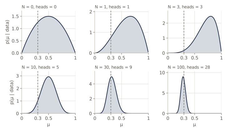
\[p(\mu \mid m, l, a, b) \propto \mu^{m} (1 - \mu)^{l} \cdot \mu^{a - 1} (1 - \mu)^{b - 1} = \mu^{m + a - 1} (1 - \mu)^{l + b - 1}.\]This is a beta density again, so we can read off its normalizing constant without integrating: the posterior is \(\operatorname{Beta}(\mu \mid a + m, b + l)\). Observing data adds the number of heads to \(a\) and the number of tails to \(b\). That gives the hyperparameters a concrete meaning: \(a\) and \(b\) act like counts of heads and tails we saw before the experiment began, pseudo-counts that need not be whole numbers.
Learning one flip at a time
Since the posterior is a beta distribution, it can serve as the prior for the next observation. Processing the data one point at a time, a head adds one to \(a\) and a tail adds one to \(b\), and after all \(N\) points we arrive at the same posterior as the batch calculation. This sequential view of Bayesian learning needs only the i.i.d. assumption: the posterior after \(n - 1\) points, times the likelihood of point \(n\), is proportional to the posterior after \(n\) points. It suits streams of data that arrive over time and data sets too large to hold in memory, since each point can be discarded once it has been absorbed.
def beta_update(a, b, x_new):
    """One step of sequential learning: heads adds 1 to a, tails adds 1 to b."""
    return a + x_new, b + (1 - x_new)

def beta_sd(a, b):
    return np.sqrt(a * b / ((a + b)**2 * (a + b + 1)))

a0, b0 = 2.0, 2.0                    # prior: a mild belief that the coin is fair
a, b = a0, b0
for n, xn in enumerate(flips, start=1):
    a, b = beta_update(a, b, xn)
    if n in (1, 3, 10, 30, 100):
        print(f"after {n:3d} flips: Beta({a:.0f}, {b:.0f}), "
              f"mean {a / (a + b):.3f}, sd {beta_sd(a, b):.3f}")
m, l = flips.sum(), len(flips) - flips.sum()
print(f"batch posterior:     Beta({a0 + m:.0f}, {b0 + l:.0f})")
after   1 flips: Beta(3, 2), mean 0.600, sd 0.200
after   3 flips: Beta(5, 2), mean 0.714, sd 0.160
after  10 flips: Beta(7, 7), mean 0.500, sd 0.129
after  30 flips: Beta(11, 23), mean 0.324, sd 0.079
after 100 flips: Beta(30, 74), mean 0.288, sd 0.044
batch posterior:     Beta(30, 74)
The predictive distribution
To predict the next flip we average the Bernoulli probability over the posterior, using the sum and product rules:
\[\begin{aligned} p(x = 1 \mid \mathcal{D}) &= \int_0^1 p(x = 1 \mid \mu) \, p(\mu \mid \mathcal{D}) \, d\mu = \int_0^1 \mu \, p(\mu \mid \mathcal{D}) \, d\mu \\ &= \mathbb{E}[\mu \mid \mathcal{D}] = \frac{m + a}{m + a + l + b}. \end{aligned}\]The prediction is the fraction of heads among all the flips, real and imaginary. Write \(N = m + l\) and rearrange:
\[\frac{m + a}{N + a + b} = \lambda \, \frac{a}{a + b} + (1 - \lambda) \, \frac{m}{N}, \qquad \lambda = \frac{a + b}{a + b + N}.\]So the posterior mean is a weighted average of the prior mean and the ML estimate, and it always lies between them. With no data, \(\lambda = 1\) and we predict with the prior; as \(N \to \infty\), \(\lambda \to 0\) and the Bayesian and ML answers agree. Agreement in the limit of infinite data is typical; the two approaches differ when data are scarce, which is exactly when it matters.
def predictive_heads(m, l, a, b):
    """p(x = 1 | D): the posterior mean of mu."""
    return (m + a) / (m + a + l + b)

for m, l in [(3, 0), (30, 0), (6, 14), (300, 700)]:
    N = m + l
    lam = (a0 + b0) / (a0 + b0 + N)                   # weight on the prior mean
    blend = lam * a0 / (a0 + b0) + (1 - lam) * m / N
    bayes = predictive_heads(m, l, a0, b0)
    print(f"m = {m:3d}, l = {l:3d}: ML {m / N:.3f}, Bayes {bayes:.3f}"
          f" = {lam:.3f} x prior mean + {1 - lam:.3f} x ML ({blend:.3f})")
m =   3, l =   0: ML 1.000, Bayes 0.714 = 0.571 x prior mean + 0.429 x ML (0.714)
m =  30, l =   0: ML 1.000, Bayes 0.941 = 0.118 x prior mean + 0.882 x ML (0.941)
m =   6, l =  14: ML 0.300, Bayes 0.333 = 0.167 x prior mean + 0.833 x ML (0.333)
m = 300, l = 700: ML 0.300, Bayes 0.301 = 0.004 x prior mean + 0.996 x ML (0.301)
After three heads in three flips (our coin’s first three), the Beta(2, 2) prior predicts heads with probability 0.714 rather than 1. After a thousand flips the prior barely matters: 0.301 against 0.300.
Does more data always shrink the posterior?
In the figure the posterior narrows as data arrive. Is that guaranteed? For any parameter \(\theta\) and data \(\mathcal{D}\) drawn from their joint distribution, two identities hold (Bishop’s exercise 2.8 asks you to prove them):
\[\mathbb{E}_{\theta}[\theta] = \mathbb{E}_{\mathcal{D}}\bigl[ \mathbb{E}_{\theta}[\theta \mid \mathcal{D}] \bigr], \qquad \operatorname{var}_{\theta}[\theta] = \mathbb{E}_{\mathcal{D}}\bigl[ \operatorname{var}_{\theta}[\theta \mid \mathcal{D}] \bigr] + \operatorname{var}_{\mathcal{D}}\bigl[ \mathbb{E}_{\theta}[\theta \mid \mathcal{D}] \bigr].\]The first says that the posterior mean, averaged over the data sets we might see, is the prior mean. The second says that the prior variance equals the average posterior variance plus a nonnegative term, so the posterior variance is, on average, no larger than the prior variance. The guarantee is only on average: a surprising data set can leave us less certain than before (exercise 3). We can watch both identities hold by simulation: draw \(\mu\) from the prior, flip that coin ten times, compute the posterior, and repeat.
rng_tv = np.random.default_rng(5)
R, N = 200_000, 10
mus = rng_tv.beta(a0, b0, size=R)              # mu from the prior
ms = rng_tv.binomial(N, mus)                   # then a data set of N flips
aN, bN = a0 + ms, b0 + N - ms
post_mean = aN / (aN + bN)
post_var = beta_sd(aN, bN)**2
print(f"prior mean {a0 / (a0 + b0):.4f}; "
      f"average posterior mean {post_mean.mean():.4f}")
print(f"prior var  {beta_sd(a0, b0)**2:.4f}; average posterior var {post_var.mean():.4f}"
      f" + var of posterior mean {post_mean.var():.4f}"
      f" = {post_var.mean() + post_mean.var():.4f}")
prior mean 0.5000; average posterior mean 0.4995
prior var  0.0500; average posterior var 0.0143 + var of posterior mean 0.0357 = 0.0500
Multinomial variables
One-of-K coding and maximum likelihood
Many discrete variables have more than two values: a die has six faces, a word comes from a vocabulary. A convenient representation for a variable with \(K\) possible states is 1-of-K coding (also called one-hot coding): a vector \(\mathbf{x}\) of length \(K\) with a single 1 in the position of the observed state and 0 everywhere else. A die showing three is \(\mathbf{x} = (0, 0, 1, 0, 0, 0)^{\mathrm{T}}\), and every such vector satisfies \(\sum_k x_k = 1\).
If state \(k\) has probability \(\mu_k\), with \(\mu_k \ge 0\) and \(\sum_k \mu_k = 1\), then
\[p(\mathbf{x} \mid \boldsymbol{\mu}) = \prod_{k=1}^{K} \mu_k^{x_k},\]because only the factor with \(x_k = 1\) survives. This generalizes the Bernoulli distribution, and \(\mathbb{E}[\mathbf{x} \mid \boldsymbol{\mu}] = \boldsymbol{\mu}\). For \(N\) independent observations the log-likelihood is
\[\ln p(\mathcal{D} \mid \boldsymbol{\mu}) = \sum_{n=1}^{N} \sum_{k=1}^{K} x_{nk} \ln \mu_k = \sum_{k=1}^{K} m_k \ln \mu_k, \qquad m_k = \sum_{n=1}^{N} x_{nk},\]so the counts \(m_k\) of each state are the sufficient statistics. To maximize it we must respect the constraint \(\sum_k \mu_k = 1\); otherwise the log-likelihood grows without bound as the \(\mu_k\) grow. A Lagrange multiplier \(\lambda\) handles the constraint (Bishop’s appendix E reviews the method): we find stationary points of
\[\sum_{k=1}^{K} m_k \ln \mu_k + \lambda \Bigl( \sum_{k=1}^{K} \mu_k - 1 \Bigr).\]The derivative with respect to \(\mu_k\) is \(m_k / \mu_k + \lambda\), which vanishes when \(\mu_k = -m_k / \lambda\). Summing over \(k\) and using the constraint gives \(1 = -N / \lambda\), so \(\lambda = -N\) and
\[\mu_k^{\mathrm{ML}} = \frac{m_k}{N},\]the observed frequency of state \(k\). We simulate 40 rolls of a loaded die and check that no other point on the probability simplex does better.
def multinomial_loglik(mu, counts):
    """sum_k m_k ln mu_k, for one mu (shape K) or many (shape (S, K))."""
    return np.sum(counts * np.log(mu), axis=-1)

rng_die = np.random.default_rng(3)
K = 6
mu_die = np.array([0.1, 0.1, 0.15, 0.15, 0.2, 0.3])
X = np.eye(K, dtype=int)[rng_die.choice(K, size=40, p=mu_die)]    # 1-of-K rows
print("first three rows:\n", X[:3])
m_k = X.sum(axis=0)
mu_ML = m_k / m_k.sum()
print("counts m_k:", m_k, "  mu_ML:", mu_ML)
others = rng_die.dirichlet(np.ones(K), size=100_000)     # random points on the simplex
print(f"log-likelihood at mu_ML {multinomial_loglik(mu_ML, m_k):.4f}; "
      f"best of 100,000 random points {multinomial_loglik(others, m_k).max():.4f}")
first three rows:
 [[1 0 0 0 0 0]
 [0 0 1 0 0 0]
 [0 0 0 0 0 1]]
counts m_k: [ 5  2  8  6  8 11]   mu_ML: [0.125 0.05  0.2   0.15  0.2   0.275]
log-likelihood at mu_ML -67.7232; best of 100,000 random points -67.8062
The joint distribution of the counts \(m_1, \dots, m_K\) given \(N\) is the multinomial distribution,
\[\operatorname{Mult}(m_1, \dots, m_K \mid \boldsymbol{\mu}, N) = \frac{N!}{m_1! \, m_2! \cdots m_K!} \prod_{k=1}^{K} \mu_k^{m_k}, \qquad \sum_{k} m_k = N,\]where the coefficient counts the ways to split \(N\) labeled observations into groups of sizes \(m_1, \dots, m_K\). With \(K = 2\) it is the binomial distribution.
The Dirichlet distribution
The conjugate prior for \(\boldsymbol{\mu}\) follows the same recipe as the beta: a product of powers of the \(\mu_k\). Normalized, it is the Dirichlet distribution
\[\operatorname{Dir}(\boldsymbol{\mu} \mid \boldsymbol{\alpha}) = \frac{\Gamma(\alpha_0)}{\Gamma(\alpha_1) \cdots \Gamma(\alpha_K)} \prod_{k=1}^{K} \mu_k^{\alpha_k - 1}, \qquad \alpha_0 = \sum_{k=1}^{K} \alpha_k,\]with all \(\alpha_k > 0\). It lives on the simplex \(\{\boldsymbol{\mu} : \mu_k \ge 0, \ \sum_k \mu_k = 1\}\), which for \(K = 3\) is a triangle, a \((K - 1)\)-dimensional region inside \(K\)-dimensional space. Its mean is \(\mathbb{E}[\mu_k] = \alpha_k / \alpha_0\). Values \(\alpha_k < 1\) push the mass toward the corners and edges of the simplex, \(\alpha_k = 1\) is uniform, and large equal \(\alpha_k\) concentrate it near the center.
Multiplying the prior by the likelihood \(\prod_k \mu_k^{m_k}\) gives
\[p(\boldsymbol{\mu} \mid \mathcal{D}, \boldsymbol{\alpha}) \propto \prod_{k=1}^{K} \mu_k^{\alpha_k + m_k - 1}, \qquad \text{so} \qquad p(\boldsymbol{\mu} \mid \mathcal{D}, \boldsymbol{\alpha}) = \operatorname{Dir}(\boldsymbol{\mu} \mid \boldsymbol{\alpha} + \mathbf{m}),\]with \(\mathbf{m} = (m_1, \dots, m_K)^{\mathrm{T}}\). As with the beta, each \(\alpha_k\) acts as a pseudo-count for state \(k\).
A convenient way to sample from a Dirichlet uses gamma variables: draw independent \(g_k\) from a gamma distribution with shape \(\alpha_k\) and scale 1 (section 3 introduces the gamma distribution), and set \(\mu_k = g_k / \sum_j g_j\). We use this to check our density and the mean, and confirm that for \(K = 2\) the Dirichlet is the beta distribution.
def dirichlet_logpdf(mu, alpha):
    """ln Dir(mu | alpha) for points mu on the simplex (last axis)."""
    return (gammaln(alpha.sum()) - gammaln(alpha).sum()
            + np.sum((alpha - 1) * np.log(mu), axis=-1))

def dirichlet_sample(alpha, size, rng):
    """Normalize independent Gamma(alpha_k, 1) draws; the result is Dir(alpha)."""
    g = rng.gamma(alpha, 1.0, size=(size, len(alpha)))
    return g / g.sum(axis=1, keepdims=True)

alpha = np.array([2.0, 3.0, 5.0])
S = dirichlet_sample(alpha, 200_000, rng)
print("sample mean:", S.mean(axis=0), "  alpha / alpha_0:", alpha / alpha.sum())
print("density matches scipy:",
      np.allclose(dirichlet_logpdf(S[:5], alpha), stats.dirichlet.logpdf(S[:5].T, alpha)))
dir2 = np.exp(dirichlet_logpdf(np.array([0.3, 0.7]), np.array([2.0, 5.0])))
beta2 = np.exp(beta_logpdf(0.3, 2, 5))
print(f"Dir((0.3, 0.7) | (2, 5)) = {dir2:.4f};  Beta(0.3 | 2, 5) = {beta2:.4f}")
sample mean: [0.1999 0.3002 0.4999]   alpha / alpha_0: [0.2 0.3 0.5]
density matches scipy: True
Dir((0.3, 0.7) | (2, 5)) = 2.1609;  Beta(0.3 | 2, 5) = 2.1609
The prior matters most when some state has not been seen yet. After the first five rolls of our die, maximum likelihood assigns probability zero to every face that has not come up, which would make any future roll of those faces “impossible”. A Dirichlet prior with \(\alpha_k = 1\) (one pseudo-count per face, also known as Laplace smoothing) keeps every face possible.
m5 = X[:5].sum(axis=0)
alpha_prior = np.ones(K)
print("counts after 5 rolls:", m5)
print("ML estimate:        ", m5 / 5)
print("posterior mean:     ", (alpha_prior + m5) / (alpha_prior.sum() + 5))
print("after all 40 rolls: ", (alpha_prior + m_k) / (alpha_prior.sum() + 40))
counts after 5 rolls: [2 0 1 0 1 1]
ML estimate:         [0.4 0.  0.2 0.  0.2 0.2]
posterior mean:      [0.2727 0.0909 0.1818 0.0909 0.1818 0.1818]
after all 40 rolls:  [0.1304 0.0652 0.1957 0.1522 0.1957 0.2609]
Watch out. A zero count gives a zero maximum likelihood probability, and a single zero in a product of probabilities wipes out the whole product. This bites in practice: a text classifier trained by ML assigns probability zero to any document that contains a word it never saw with that class. Pseudo-counts from a Dirichlet prior are the standard remedy.
The Gaussian distribution
The Gaussian (or normal) distribution of a single real variable is
\[\mathcal{N}(x \mid \mu, \sigma^2) = \frac{1}{(2\pi\sigma^2)^{1/2}} \exp\Bigl\{ -\frac{1}{2\sigma^2} (x - \mu)^2 \Bigr\},\]with mean \(\mu\) and variance \(\sigma^2\). For a \(D\)-dimensional vector \(\mathbf{x}\) the multivariate Gaussian is
\[\mathcal{N}(\mathbf{x} \mid \boldsymbol{\mu}, \boldsymbol{\Sigma}) = \frac{1}{(2\pi)^{D/2}} \frac{1}{\lvert \boldsymbol{\Sigma} \rvert^{1/2}} \exp\Bigl\{ -\frac{1}{2} (\mathbf{x} - \boldsymbol{\mu})^{\mathrm{T}} \boldsymbol{\Sigma}^{-1} (\mathbf{x} - \boldsymbol{\mu}) \Bigr\},\]where \(\boldsymbol{\mu}\) is a \(D\)-vector, \(\boldsymbol{\Sigma}\) is a \(D \times D\) symmetric positive definite matrix, and \(\lvert \boldsymbol{\Sigma} \rvert\) is its determinant.
Why this distribution, over and over? One reason comes from information theory (Bishop §1.6, and module 01): among all densities with a given mean and variance, the Gaussian has the largest entropy, so it assumes the least beyond those two moments (the same holds in \(D\) dimensions for a given covariance). Another is the central limit theorem: under mild conditions, a sum of many independent random variables is approximately Gaussian, whatever the distribution of the terms. Measurement errors that come from many small independent causes tend to look Gaussian for this reason, and the binomial count \(m\), a sum of Bernoulli variables, becomes Gaussian-shaped as \(N\) grows. The convergence can be fast. Here we average \(N\) uniform numbers on \([0, 1]\), standardize, and compare two tail probabilities with the Gaussian values.
rng_clt = np.random.default_rng(4)
for n in (1, 2, 10):
    means = rng_clt.random((200_000, n)).mean(axis=1)
    z = (means - 0.5) / np.sqrt(1 / (12 * n))   # a uniform on [0, 1] has variance 1/12
    p1, p2 = np.mean(np.abs(z) < 1), np.mean(np.abs(z) < 2)
    print(f"N = {n:2d}: P(|z| < 1) = {p1:.4f}, P(|z| < 2) = {p2:.4f}")
g1, g2 = 2 * stats.norm.cdf(1) - 1, 2 * stats.norm.cdf(2) - 1
print(f"Gaussian: P(|z| < 1) = {g1:.4f}, P(|z| < 2) = {g2:.4f}")
N =  1: P(|z| < 1) = 0.5766, P(|z| < 2) = 1.0000
N =  2: P(|z| < 1) = 0.6490, P(|z| < 2) = 0.9667
N = 10: P(|z| < 1) = 0.6782, P(|z| < 2) = 0.9556
Gaussian: P(|z| < 1) = 0.6827, P(|z| < 2) = 0.9545
With ten terms the probabilities are already within about 0.005 of the Gaussian values. The rest of this section develops the Gaussian’s properties in detail. It is the most technical part of the module, and the part the rest of the course uses most.
Geometry: eigenvectors and Mahalanobis distance
The Gaussian depends on \(\mathbf{x}\) only through the quadratic form
\[\Delta^2 = (\mathbf{x} - \boldsymbol{\mu})^{\mathrm{T}} \boldsymbol{\Sigma}^{-1} (\mathbf{x} - \boldsymbol{\mu}).\]The quantity \(\Delta\) is the Mahalanobis distance from \(\boldsymbol{\mu}\) to \(\mathbf{x}\). When \(\boldsymbol{\Sigma} = \mathbf{I}\) it is the ordinary Euclidean distance; in general it measures distance in units that account for the spread of the distribution in each direction. The density is constant wherever \(\Delta\) is constant. We can take \(\boldsymbol{\Sigma}\) symmetric without losing anything, since an antisymmetric part of \(\boldsymbol{\Sigma}^{-1}\) would cancel in the quadratic form.
To see what the surfaces of constant \(\Delta\) look like, use the eigenvectors of the covariance. Because \(\boldsymbol{\Sigma}\) is real and symmetric, it has real eigenvalues \(\lambda_i\) and orthonormal eigenvectors \(\mathbf{u}_i\):
\[\boldsymbol{\Sigma} \mathbf{u}_i = \lambda_i \mathbf{u}_i, \qquad \mathbf{u}_i^{\mathrm{T}} \mathbf{u}_j = \begin{cases} 1 & i = j \\ 0 & i \ne j. \end{cases}\]Collect the eigenvectors as the columns of an orthogonal matrix \(\mathbf{U}\) (so \(\mathbf{U}^{\mathrm{T}} \mathbf{U} = \mathbf{U} \mathbf{U}^{\mathrm{T}} = \mathbf{I}\)). Then \(\boldsymbol{\Sigma} = \sum_i \lambda_i \mathbf{u}_i \mathbf{u}_i^{\mathrm{T}}\) and \(\boldsymbol{\Sigma}^{-1} = \sum_i \lambda_i^{-1} \mathbf{u}_i \mathbf{u}_i^{\mathrm{T}}\). Define new coordinates \(y_i = \mathbf{u}_i^{\mathrm{T}} (\mathbf{x} - \boldsymbol{\mu})\), that is, \(\mathbf{y} = \mathbf{U}^{\mathrm{T}} (\mathbf{x} - \boldsymbol{\mu})\): shift the origin to the mean and rotate the axes onto the eigenvectors. (Bishop stacks the eigenvectors as rows instead, so his \(\mathbf{U}\) is our \(\mathbf{U}^{\mathrm{T}}\).) In these coordinates the quadratic form has no cross terms:
\[\Delta^2 = \sum_{i=1}^{D} \frac{y_i^2}{\lambda_i}.\]So the surfaces of constant density are ellipsoids centered at \(\boldsymbol{\mu}\), with axes along the eigenvectors and half-lengths proportional to \(\lambda_i^{1/2}\). For this to describe a proper distribution every \(\lambda_i\) must be strictly positive; a matrix with that property is positive definite. (If some eigenvalues are zero, the matrix is positive semidefinite and the distribution is squashed onto a lower-dimensional subspace, a case that returns in module 12.)
The change of variables also shows that the density is normalized. The map from \(\mathbf{x}\) to \(\mathbf{y}\) is a rotation plus a shift, so its Jacobian determinant has absolute value 1, and \(\lvert \boldsymbol{\Sigma} \rvert = \prod_j \lambda_j\). Substituting,
\[p(\mathbf{y}) = \prod_{j=1}^{D} \frac{1}{(2\pi\lambda_j)^{1/2}} \exp\Bigl\{ -\frac{y_j^2}{2\lambda_j} \Bigr\},\]a product of \(D\) independent one-dimensional Gaussians with variances \(\lambda_j\). Each factor integrates to one, so the whole density does. In the eigenvector coordinates a correlated Gaussian is just \(D\) independent ones.
We evaluate the density through the Cholesky factorization \(\boldsymbol{\Sigma} = \mathbf{L} \mathbf{L}^{\mathrm{T}}\), with \(\mathbf{L}\) lower triangular. Then \(\Delta^2 = \lVert \mathbf{L}^{-1} (\mathbf{x} - \boldsymbol{\mu}) \rVert^2\), which one triangular solve gives us, and \(\ln \lvert \boldsymbol{\Sigma} \rvert = 2 \sum_i \ln L_{ii}\).
def gaussian_logpdf(X, mu, Sigma):
    """ln N(x | mu, Sigma) for each row x of X, via Cholesky: Sigma = L L^T."""
    X = np.atleast_2d(X)
    D = X.shape[1]
    L = np.linalg.cholesky(Sigma)
    z = solve_triangular(L, (X - mu).T, lower=True)      # z = L^{-1} (x - mu)
    maha2 = np.sum(z**2, axis=0)                          # Delta^2 = z^T z
    log_det = 2 * np.sum(np.log(np.diag(L)))              # ln |Sigma|
    return -0.5 * (D * np.log(2 * np.pi) + log_det + maha2)

mu = np.array([1.0, 0.5])
Sigma = np.array([[2.0, 1.2],
                  [1.2, 1.5]])
lam, U = np.linalg.eigh(Sigma)          # eigenvalues ascending; columns of U are u_i
print("eigenvalues:", lam, "\neigenvectors (columns):\n", U)
print("U orthogonal:", np.allclose(U.T @ U, np.eye(2)),
      "  Sigma = sum lam_i u_i u_i^T:", np.allclose((U * lam) @ U.T, Sigma))

x = np.array([2.5, -0.5])
y = U.T @ (x - mu)                          # eigenvector coordinates
print(f"Delta^2 = {(x - mu) @ np.linalg.solve(Sigma, x - mu):.4f} directly, "
      f"{np.sum(y**2 / lam):.4f} from the y_i; "
      f"squared Euclidean distance {np.sum((x - mu)**2):.4f}")

pts = rng.normal(size=(4, 2)) * 2
Y = (pts - mu) @ U                          # row n holds y for point n
print("ln N(x):              ", gaussian_logpdf(pts, mu, Sigma))
print("sum of 1-D log terms: ",
      np.sum(-0.5 * np.log(2 * np.pi * lam) - Y**2 / (2 * lam), axis=1))
ref = stats.multivariate_normal(mu, Sigma).logpdf(pts)
print("matches scipy:", np.allclose(gaussian_logpdf(pts, mu, Sigma), ref))
eigenvalues: [0.5242 2.9758]
eigenvectors (columns):
 [[ 0.6309 -0.7759]
 [-0.7759 -0.6309]]
U orthogonal: True   Sigma = sum lam_i u_i u_i^T: True
Delta^2 = 5.7532 directly, 5.7532 from the y_i; squared Euclidean distance 3.2500
ln N(x):               [-2.1717 -3.221  -4.5167 -6.3914]
sum of 1-D log terms:  [-2.1717 -3.221  -4.5167 -6.3914]
matches scipy: True
The point \(\mathbf{x} = (2.5, -0.5)\) is at Euclidean distance 1.80 from the mean but Mahalanobis distance \(\sqrt{5.75} \approx 2.40\): it lies across the direction in which the distribution is narrow. The long axis of the ellipse points along the eigenvector with the larger eigenvalue, 2.98, which is \(\pm(0.78, 0.63)\), tilted about 39 degrees above the \(x_1\) axis (an eigenvector’s sign is arbitrary, and NumPy happened to return the negative one).
Moments
The parameters are named for what they are. For the mean, substitute \(\mathbf{z} = \mathbf{x} - \boldsymbol{\mu}\) in \(\mathbb{E}[\mathbf{x}] = \int \mathcal{N}(\mathbf{x} \mid \boldsymbol{\mu}, \boldsymbol{\Sigma}) \, \mathbf{x} \, d\mathbf{x}\). The density is an even function of \(\mathbf{z}\), so the integral of \(\mathbf{z}\) times it vanishes, and what remains is \(\boldsymbol{\mu}\) times the integral of the density:
\[\mathbb{E}[\mathbf{x}] = \boldsymbol{\mu}.\]For the second moments \(\mathbb{E}[\mathbf{x}\mathbf{x}^{\mathrm{T}}]\), the same substitution leaves \(\boldsymbol{\mu}\boldsymbol{\mu}^{\mathrm{T}}\) (the cross terms vanish by symmetry) plus \(\mathbb{E}[\mathbf{z}\mathbf{z}^{\mathrm{T}}]\). Expanding \(\mathbf{z} = \sum_j y_j \mathbf{u}_j\) in the eigenvectors, the \(y_j\) are independent with mean 0 and variance \(\lambda_j\), so
\[\mathbb{E}[\mathbf{z}\mathbf{z}^{\mathrm{T}}] = \sum_{i,j} \mathbb{E}[y_i y_j] \, \mathbf{u}_i \mathbf{u}_j^{\mathrm{T}} = \sum_i \lambda_i \mathbf{u}_i \mathbf{u}_i^{\mathrm{T}} = \boldsymbol{\Sigma}.\]Hence
\[\mathbb{E}[\mathbf{x}\mathbf{x}^{\mathrm{T}}] = \boldsymbol{\mu}\boldsymbol{\mu}^{\mathrm{T}} + \boldsymbol{\Sigma}, \qquad \operatorname{cov}[\mathbf{x}] = \mathbb{E}\bigl[(\mathbf{x} - \mathbb{E}[\mathbf{x}])(\mathbf{x} - \mathbb{E}[\mathbf{x}])^{\mathrm{T}}\bigr] = \boldsymbol{\Sigma},\]which is why \(\boldsymbol{\Sigma}\) is called the covariance matrix. The same factorization gives a sampler: if \(\mathbf{z}\) has independent standard normal entries, then \(\mathbf{x} = \boldsymbol{\mu} + \mathbf{L}\mathbf{z}\) has mean \(\boldsymbol{\mu}\) and covariance \(\mathbf{L}\mathbf{L}^{\mathrm{T}} = \boldsymbol{\Sigma}\).
def gaussian_sample(mu, Sigma, size, rng):
    """x = mu + L z with z standard normal, so cov[x] = L L^T = Sigma."""
    L = np.linalg.cholesky(Sigma)
    return mu + rng.standard_normal((size, len(mu))) @ L.T

S = gaussian_sample(mu, Sigma, 400_000, rng)
print("E[x] estimate:     ", S.mean(axis=0))
print("E[x x^T] estimate:\n", S.T @ S / len(S))
print("mu mu^T + Sigma:\n", np.outer(mu, mu) + Sigma)
z = solve_triangular(np.linalg.cholesky(Sigma), (S - mu).T, lower=True)
d2 = np.sum(z**2, axis=0)                                   # Delta^2 for every sample
print(f"fraction with Delta <= 1: {np.mean(d2 <= 1):.4f}  "
      f"(in 2-D this is 1 - exp(-1/2) = {1 - np.exp(-0.5):.4f})")
E[x] estimate:      [0.9996 0.5004]
E[x x^T] estimate:
 [[2.9963 1.6989]
 [1.6989 1.7508]]
mu mu^T + Sigma:
 [[3.   1.7 ]
 [1.7  1.75]]
fraction with Delta <= 1: 0.3939  (in 2-D this is 1 - exp(-1/2) = 0.3935)
The last line is a useful calibration: in two dimensions only about 39% of the probability lies inside the ellipse \(\Delta = 1\), compared with 68% within one standard deviation in one dimension. (In general \(\Delta^2\) has a chi-squared distribution with \(D\) degrees of freedom, so the fraction inside \(\Delta = 1\) shrinks quickly as \(D\) grows.)
How many parameters?
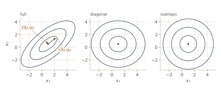
A general symmetric \(\boldsymbol{\Sigma}\) has \(D(D + 1)/2\) free entries, and \(\boldsymbol{\mu}\) adds \(D\) more, for \(D(D + 3)/2\) in total. That grows quadratically with the dimension, and inverting or factorizing \(\boldsymbol{\Sigma}\) costs \(O(D^3)\). Two restricted forms are common:
| Covariance | Form | Parameters (with the mean) | Contours | \(D = 10\) | \(D = 784\) |
|---|---|---|---|---|---|
| full | any positive definite \(\boldsymbol{\Sigma}\) | \(D(D + 3)/2\) | tilted ellipsoids | 65 | 308,504 |
| diagonal | \(\operatorname{diag}(\sigma_1^2, \dots, \sigma_D^2)\) | \(2D\) | axis-aligned ellipsoids | 20 | 1,568 |
| isotropic | \(\sigma^2 \mathbf{I}\) | \(D + 1\) | spheres | 11 | 785 |
(784 is the number of pixels in a 28 × 28 image.) The restricted forms are cheaper to store, fit, and invert, but they cannot express correlations between variables. The best diagonal approximation to our example keeps the diagonal of \(\boldsymbol{\Sigma}\), and the best isotropic one uses the average variance \(\operatorname{tr}(\boldsymbol{\Sigma}) / D\) on the diagonal (these are what maximum likelihood fits of the restricted forms converge to when the data come from the full Gaussian; see exercise 5). We compare the three on the samples drawn above.
Sigma_diag = np.diag(np.diag(Sigma))
Sigma_iso = np.trace(Sigma) / 2 * np.eye(2)
for name, C in [("full", Sigma), ("diagonal", Sigma_diag), ("isotropic", Sigma_iso)]:
    avg = gaussian_logpdf(S, mu, C).mean()
    print(f"{name:9s}: average log-likelihood per point {avg:.4f}")
full     : average log-likelihood per point -3.0602
diagonal : average log-likelihood per point -3.3866
isotropic: average log-likelihood per point -3.3968
Ignoring the correlation costs about 0.33 nats of log-likelihood per point. Forcing the two variances to be equal as well costs little more here, because they are similar (2.0 and 1.5).
A second limitation is that the Gaussian has a single peak. It cannot represent data that fall into several clumps. So the Gaussian can be too flexible (too many parameters) and too rigid (one peak) at the same time. Latent variables address both: mixtures of Gaussians (end of this section, and module 09) give many peaks, and continuous latent-variable models such as probabilistic PCA (module 12) capture the main correlations with far fewer than \(D^2\) parameters. Graphical models (module 08) impose structure on very large Gaussians, as the linear dynamical system of module 13 does over time.
Conditional Gaussians
A key property: when two groups of variables have a joint Gaussian distribution, fixing one group leaves a Gaussian over the other, and integrating one group out also leaves a Gaussian. We now derive both, because the same algebra appears in regression, Gaussian processes, and the Kalman filter.
Split \(\mathbf{x}\) into two parts, \(\mathbf{x}_a\) (the first \(M\) components) and \(\mathbf{x}_b\) (the other \(D - M\)), and partition the mean and covariance to match:
\[\mathbf{x} = \begin{pmatrix} \mathbf{x}_a \\ \mathbf{x}_b \end{pmatrix}, \qquad \boldsymbol{\mu} = \begin{pmatrix} \boldsymbol{\mu}_a \\ \boldsymbol{\mu}_b \end{pmatrix}, \qquad \boldsymbol{\Sigma} = \begin{pmatrix} \boldsymbol{\Sigma}_{aa} & \boldsymbol{\Sigma}_{ab} \\ \boldsymbol{\Sigma}_{ba} & \boldsymbol{\Sigma}_{bb} \end{pmatrix}.\]Symmetry of \(\boldsymbol{\Sigma}\) means \(\boldsymbol{\Sigma}_{aa}\) and \(\boldsymbol{\Sigma}_{bb}\) are symmetric and \(\boldsymbol{\Sigma}_{ba} = \boldsymbol{\Sigma}_{ab}^{\mathrm{T}}\). It will pay to work also with the inverse of the covariance, the precision matrix \(\boldsymbol{\Lambda} = \boldsymbol{\Sigma}^{-1}\), partitioned the same way into \(\boldsymbol{\Lambda}_{aa}, \boldsymbol{\Lambda}_{ab}, \boldsymbol{\Lambda}_{ba}, \boldsymbol{\Lambda}_{bb}\) (again with \(\boldsymbol{\Lambda}_{ba} = \boldsymbol{\Lambda}_{ab}^{\mathrm{T}}\)).
Watch out. The blocks of the precision matrix are not the inverses of the blocks of the covariance: in general \(\boldsymbol{\Lambda}_{aa} \ne \boldsymbol{\Sigma}_{aa}^{-1}\). Inverting a block matrix mixes all of its blocks, as the formula below shows.
By the product rule, \(p(\mathbf{x}_a \mid \mathbf{x}_b) = p(\mathbf{x}_a, \mathbf{x}_b) / p(\mathbf{x}_b)\). As a function of \(\mathbf{x}_a\), with \(\mathbf{x}_b\) held fixed at its observed value, the denominator is a constant. So the conditional is the joint density, viewed as a function of \(\mathbf{x}_a\) alone and renormalized. We never need to do the normalizing integral, thanks to a simple recipe.
Note. Completing the square. The exponent of any Gaussian \(\mathcal{N}(\mathbf{x} \mid \mathbf{m}, \mathbf{C})\), expanded, is \(-\frac{1}{2} \mathbf{x}^{\mathrm{T}} \mathbf{C}^{-1} \mathbf{x} + \mathbf{x}^{\mathrm{T}} \mathbf{C}^{-1} \mathbf{m} + \text{const}\). So if some log-density is a quadratic function of \(\mathbf{x}\) (with a negative definite second-order part), it is Gaussian, and we can read off its parameters: the matrix in the second-order term is the precision \(\mathbf{C}^{-1}\), and the vector in the first-order term is \(\mathbf{C}^{-1} \mathbf{m}\), which gives the mean. Constants, including the normalizer, take care of themselves.
Write the joint exponent with the partitioned precision. Since \(\boldsymbol{\Lambda}_{ba} = \boldsymbol{\Lambda}_{ab}^{\mathrm{T}}\), the two cross terms are equal and combine:
\[\begin{aligned} -\frac{1}{2} (\mathbf{x} - \boldsymbol{\mu})^{\mathrm{T}} \boldsymbol{\Lambda} (\mathbf{x} - \boldsymbol{\mu}) = &-\frac{1}{2} (\mathbf{x}_a - \boldsymbol{\mu}_a)^{\mathrm{T}} \boldsymbol{\Lambda}_{aa} (\mathbf{x}_a - \boldsymbol{\mu}_a) \\ &- (\mathbf{x}_a - \boldsymbol{\mu}_a)^{\mathrm{T}} \boldsymbol{\Lambda}_{ab} (\mathbf{x}_b - \boldsymbol{\mu}_b) \\ &- \frac{1}{2} (\mathbf{x}_b - \boldsymbol{\mu}_b)^{\mathrm{T}} \boldsymbol{\Lambda}_{bb} (\mathbf{x}_b - \boldsymbol{\mu}_b). \end{aligned}\]This is quadratic in \(\mathbf{x}_a\), so the conditional is Gaussian. Its second-order term in \(\mathbf{x}_a\) is \(-\frac{1}{2} \mathbf{x}_a^{\mathrm{T}} \boldsymbol{\Lambda}_{aa} \mathbf{x}_a\), so the conditional precision is \(\boldsymbol{\Lambda}_{aa}\). Its first-order terms are \(\mathbf{x}_a^{\mathrm{T}} \{ \boldsymbol{\Lambda}_{aa} \boldsymbol{\mu}_a - \boldsymbol{\Lambda}_{ab} (\mathbf{x}_b - \boldsymbol{\mu}_b) \}\), and this vector must equal the precision times the conditional mean. Therefore
\[\boldsymbol{\Sigma}_{a \mid b} = \boldsymbol{\Lambda}_{aa}^{-1}, \qquad \boldsymbol{\mu}_{a \mid b} = \boldsymbol{\mu}_a - \boldsymbol{\Lambda}_{aa}^{-1} \boldsymbol{\Lambda}_{ab} (\mathbf{x}_b - \boldsymbol{\mu}_b).\]To express this in terms of the covariance blocks we need the inverse of a partitioned matrix. For any invertible block matrix, with \(\mathbf{M} = (\mathbf{A} - \mathbf{B}\mathbf{D}^{-1}\mathbf{C})^{-1}\),
\[\begin{pmatrix} \mathbf{A} & \mathbf{B} \\ \mathbf{C} & \mathbf{D} \end{pmatrix}^{-1} = \begin{pmatrix} \mathbf{M} & -\mathbf{M}\mathbf{B}\mathbf{D}^{-1} \\ -\mathbf{D}^{-1}\mathbf{C}\mathbf{M} & \mathbf{D}^{-1} + \mathbf{D}^{-1}\mathbf{C}\mathbf{M}\mathbf{B}\mathbf{D}^{-1} \end{pmatrix},\]which you can verify by multiplying out (exercise 6). The matrix \(\mathbf{M}^{-1} = \mathbf{A} - \mathbf{B}\mathbf{D}^{-1}\mathbf{C}\) is called the Schur complement of \(\mathbf{D}\). Applying the formula to \(\boldsymbol{\Sigma}\), whose inverse is \(\boldsymbol{\Lambda}\), gives \(\boldsymbol{\Lambda}_{aa} = (\boldsymbol{\Sigma}_{aa} - \boldsymbol{\Sigma}_{ab}\boldsymbol{\Sigma}_{bb}^{-1}\boldsymbol{\Sigma}_{ba})^{-1}\) and \(\boldsymbol{\Lambda}_{ab} = -\boldsymbol{\Lambda}_{aa} \boldsymbol{\Sigma}_{ab} \boldsymbol{\Sigma}_{bb}^{-1}\). Substituting, \(-\boldsymbol{\Lambda}_{aa}^{-1}\boldsymbol{\Lambda}_{ab} = \boldsymbol{\Sigma}_{ab}\boldsymbol{\Sigma}_{bb}^{-1}\), and so
\[\boldsymbol{\mu}_{a \mid b} = \boldsymbol{\mu}_a + \boldsymbol{\Sigma}_{ab} \boldsymbol{\Sigma}_{bb}^{-1} (\mathbf{x}_b - \boldsymbol{\mu}_b), \qquad \boldsymbol{\Sigma}_{a \mid b} = \boldsymbol{\Sigma}_{aa} - \boldsymbol{\Sigma}_{ab} \boldsymbol{\Sigma}_{bb}^{-1} \boldsymbol{\Sigma}_{ba}.\]Three things to notice. The conditional mean is a linear function of \(\mathbf{x}_b\): observing \(\mathbf{x}_b\) above its mean shifts our estimate of \(\mathbf{x}_a\) by an amount proportional to the covariance between them. The conditional covariance does not depend on the observed value \(\mathbf{x}_b\) at all. And it is never larger than the marginal covariance \(\boldsymbol{\Sigma}_{aa}\), since we subtract a positive semidefinite matrix: observing correlated variables can only sharpen our knowledge. A model in which a Gaussian’s mean depends linearly on another variable while its covariance stays fixed is called a linear-Gaussian model.
Marginal Gaussians
Now integrate out \(\mathbf{x}_b\): \(p(\mathbf{x}_a) = \int p(\mathbf{x}_a, \mathbf{x}_b) \, d\mathbf{x}_b\). The plan is to complete the square in \(\mathbf{x}_b\), so that the integral becomes the integral of an unnormalized Gaussian, which is a constant. The terms in the joint exponent that involve \(\mathbf{x}_b\) are \(-\frac{1}{2} \mathbf{x}_b^{\mathrm{T}} \boldsymbol{\Lambda}_{bb} \mathbf{x}_b + \mathbf{x}_b^{\mathrm{T}} \mathbf{m}\), where \(\mathbf{m} = \boldsymbol{\Lambda}_{bb} \boldsymbol{\mu}_b - \boldsymbol{\Lambda}_{ba} (\mathbf{x}_a - \boldsymbol{\mu}_a)\) collects everything that multiplies \(\mathbf{x}_b\) linearly. Completing the square,
\[\begin{aligned} -\frac{1}{2} \mathbf{x}_b^{\mathrm{T}} \boldsymbol{\Lambda}_{bb} \mathbf{x}_b + \mathbf{x}_b^{\mathrm{T}} \mathbf{m} = &-\frac{1}{2} (\mathbf{x}_b - \boldsymbol{\Lambda}_{bb}^{-1}\mathbf{m})^{\mathrm{T}} \boldsymbol{\Lambda}_{bb} (\mathbf{x}_b - \boldsymbol{\Lambda}_{bb}^{-1}\mathbf{m}) \\ &+ \frac{1}{2} \mathbf{m}^{\mathrm{T}} \boldsymbol{\Lambda}_{bb}^{-1} \mathbf{m}. \end{aligned}\]The first term on the right is the exponent of a Gaussian in \(\mathbf{x}_b\). Its integral is the reciprocal of a Gaussian normalizer, which depends only on \(\boldsymbol{\Lambda}_{bb}\) and not on \(\mathbf{x}_a\). So after integrating, the \(\mathbf{x}_a\)-dependence comes from \(\frac{1}{2}\mathbf{m}^{\mathrm{T}}\boldsymbol{\Lambda}_{bb}^{-1}\mathbf{m}\) together with the terms of the joint exponent that involve only \(\mathbf{x}_a\), namely \(-\frac{1}{2}\mathbf{x}_a^{\mathrm{T}}\boldsymbol{\Lambda}_{aa}\mathbf{x}_a + \mathbf{x}_a^{\mathrm{T}}(\boldsymbol{\Lambda}_{aa}\boldsymbol{\mu}_a + \boldsymbol{\Lambda}_{ab}\boldsymbol{\mu}_b)\). Expanding \(\mathbf{m}\) and collecting,
\[-\frac{1}{2} \mathbf{x}_a^{\mathrm{T}} (\boldsymbol{\Lambda}_{aa} - \boldsymbol{\Lambda}_{ab}\boldsymbol{\Lambda}_{bb}^{-1}\boldsymbol{\Lambda}_{ba}) \mathbf{x}_a + \mathbf{x}_a^{\mathrm{T}} (\boldsymbol{\Lambda}_{aa} - \boldsymbol{\Lambda}_{ab}\boldsymbol{\Lambda}_{bb}^{-1}\boldsymbol{\Lambda}_{ba}) \boldsymbol{\mu}_a + \text{const}.\](The \(\boldsymbol{\mu}_b\) terms cancel.) By the recipe, the marginal has precision \(\boldsymbol{\Lambda}_{aa} - \boldsymbol{\Lambda}_{ab}\boldsymbol{\Lambda}_{bb}^{-1}\boldsymbol{\Lambda}_{ba}\) and mean \(\boldsymbol{\mu}_a\). The partitioned-inverse formula, now applied to \(\boldsymbol{\Lambda}\) (whose inverse is \(\boldsymbol{\Sigma}\)), says that the inverse of this Schur complement is exactly the top-left block \(\boldsymbol{\Sigma}_{aa}\). The marginal is as simple as one could hope.
Result. Partitioned Gaussians. If \(p(\mathbf{x}) = \mathcal{N}(\mathbf{x} \mid \boldsymbol{\mu}, \boldsymbol{\Sigma})\) with \(\mathbf{x}\), \(\boldsymbol{\mu}\), \(\boldsymbol{\Sigma}\), and \(\boldsymbol{\Lambda} = \boldsymbol{\Sigma}^{-1}\) partitioned as above, then
\[p(\mathbf{x}_a) = \mathcal{N}(\mathbf{x}_a \mid \boldsymbol{\mu}_a, \boldsymbol{\Sigma}_{aa}), \qquad p(\mathbf{x}_a \mid \mathbf{x}_b) = \mathcal{N}(\mathbf{x}_a \mid \boldsymbol{\mu}_{a \mid b}, \boldsymbol{\Sigma}_{a \mid b}),\]where
\[\begin{aligned} \boldsymbol{\mu}_{a \mid b} &= \boldsymbol{\mu}_a + \boldsymbol{\Sigma}_{ab}\boldsymbol{\Sigma}_{bb}^{-1}(\mathbf{x}_b - \boldsymbol{\mu}_b) = \boldsymbol{\mu}_a - \boldsymbol{\Lambda}_{aa}^{-1}\boldsymbol{\Lambda}_{ab}(\mathbf{x}_b - \boldsymbol{\mu}_b), \\ \boldsymbol{\Sigma}_{a \mid b} &= \boldsymbol{\Sigma}_{aa} - \boldsymbol{\Sigma}_{ab}\boldsymbol{\Sigma}_{bb}^{-1}\boldsymbol{\Sigma}_{ba} = \boldsymbol{\Lambda}_{aa}^{-1}. \end{aligned}\]Marginals are simplest in the covariance blocks; conditionals are simplest in the precision blocks.
We implement the conditional both ways and check them against each other and against brute force: draw two million samples from a three-dimensional Gaussian, keep the ones whose last coordinate lands within 0.02 of the conditioning value, and look at the mean and covariance of the first two coordinates among the survivors.
def gaussian_conditional(mu, Sigma, a, b, x_b):
    """Mean and covariance of p(x_a | x_b) from the covariance blocks."""
    S_aa, S_ab, S_bb = Sigma[np.ix_(a, a)], Sigma[np.ix_(a, b)], Sigma[np.ix_(b, b)]
    G = np.linalg.solve(S_bb, S_ab.T).T            # Sigma_ab Sigma_bb^{-1}, no inverse
    return mu[a] + G @ (x_b - mu[b]), S_aa - G @ S_ab.T

def gaussian_conditional_precision(mu, Sigma, a, b, x_b):
    """The same from the precision blocks (Lambda formed only to mirror the formula)."""
    Lam = np.linalg.inv(Sigma)
    L_aa, L_ab = Lam[np.ix_(a, a)], Lam[np.ix_(a, b)]
    return mu[a] - np.linalg.solve(L_aa, L_ab @ (x_b - mu[b])), np.linalg.inv(L_aa)

mu3 = np.array([0.0, 1.0, -1.0])
Sigma3 = np.array([[1.0,  0.6,  0.5],
                   [0.6,  2.0, -0.4],
                   [0.5, -0.4,  1.5]])
a, b, x_b = [0, 1], [2], np.array([0.0])
m1, C1 = gaussian_conditional(mu3, Sigma3, a, b, x_b)
m2, C2 = gaussian_conditional_precision(mu3, Sigma3, a, b, x_b)
print("mu_a|b =", m1, "\nSigma_a|b =\n", C1)
print("covariance and precision forms agree:",
      np.allclose(m1, m2) and np.allclose(C1, C2))

S3 = gaussian_sample(mu3, Sigma3, 2_000_000, rng)
near = np.abs(S3[:, 2] - x_b[0]) < 0.02
print(f"{near.sum()} samples with x_3 within 0.02 of 0")
kept = S3[near][:, a]
print("their mean of x_a:", kept.mean(axis=0), "\ntheir covariance:\n", np.cov(kept.T))
print("marginal: covariance of x_a over all samples\n", np.cov(S3[:, a].T),
      "\nSigma_aa\n", Sigma3[np.ix_(a, a)])
mu_a|b = [0.3333 0.7333]
Sigma_a|b =
 [[0.8333 0.7333]
 [0.7333 1.8933]]
covariance and precision forms agree: True
18816 samples with x_3 within 0.02 of 0
their mean of x_a: [0.3259 0.7237]
their covariance:
 [[0.8466 0.7459]
 [0.7459 1.9032]]
marginal: covariance of x_a over all samples
 [[0.9998 0.6001]
 [0.6001 2.0022]]
Sigma_aa
 [[1.  0.6]
 [0.6 2. ]]
The sampled conditional mean and covariance agree with the formulas to within Monte Carlo error (18,816 samples survive the filter), and the plain sample covariance of \(\mathbf{x}_a\) reproduces \(\boldsymbol{\Sigma}_{aa}\). Observing \(x_3 = 0\), which is one unit above its mean of \(-1\), pulls \(x_1\) up (their covariance is positive) and \(x_2\) down (theirs is negative), and shrinks both variances.
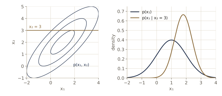
A two-dimensional example makes the picture concrete. With unit variances and correlation 0.8, observing \(x_b\) one standard deviation above its mean moves the conditional mean of \(x_a\) by 0.8 and shrinks its variance from 1 to \(1 - 0.8^2 = 0.36\).
mu2 = np.array([1.0, 2.0])
Sigma2 = np.array([[1.0, 0.8],
                   [0.8, 1.0]])
mc, Cc = gaussian_conditional(mu2, Sigma2, [0], [1], np.array([3.0]))
print(f"p(x_a):           mean {mu2[0]:.2f}, sd {np.sqrt(Sigma2[0, 0]):.2f}")
print(f"p(x_a | x_b = 3): mean {mc[0]:.2f}, sd {np.sqrt(Cc[0, 0]):.2f}")
p(x_a):           mean 1.00, sd 1.00
p(x_a | x_b = 3): mean 1.80, sd 0.60
Bayes’ theorem for linear-Gaussian models
The partitioned results start from a joint Gaussian. In practice a model usually comes the other way around: a prior over some unknown \(\mathbf{x}\), and a description of how an observation \(\mathbf{y}\) is generated from \(\mathbf{x}\). Suppose
\[p(\mathbf{x}) = \mathcal{N}(\mathbf{x} \mid \boldsymbol{\mu}, \boldsymbol{\Lambda}^{-1}), \qquad p(\mathbf{y} \mid \mathbf{x}) = \mathcal{N}(\mathbf{y} \mid \mathbf{A}\mathbf{x} + \mathbf{b}, \mathbf{L}^{-1}),\]with \(\mathbf{x}\) of dimension \(M\), \(\mathbf{y}\) of dimension \(D\), \(\mathbf{A}\) a \(D \times M\) matrix, and precisions \(\boldsymbol{\Lambda}\) and \(\mathbf{L}\). Equivalently, \(\mathbf{y} = \mathbf{A}\mathbf{x} + \mathbf{b} + \boldsymbol{\epsilon}\), where the noise \(\boldsymbol{\epsilon}\) is Gaussian with zero mean and covariance \(\mathbf{L}^{-1}\), independent of \(\mathbf{x}\). We want the two quantities Bayes’ theorem needs: the evidence \(p(\mathbf{y})\) and the posterior \(p(\mathbf{x} \mid \mathbf{y})\).
First the joint distribution of \(\mathbf{z} = (\mathbf{x}, \mathbf{y})\). Its log is
\[\ln p(\mathbf{z}) = -\frac{1}{2} (\mathbf{x} - \boldsymbol{\mu})^{\mathrm{T}} \boldsymbol{\Lambda} (\mathbf{x} - \boldsymbol{\mu}) - \frac{1}{2} (\mathbf{y} - \mathbf{A}\mathbf{x} - \mathbf{b})^{\mathrm{T}} \mathbf{L} (\mathbf{y} - \mathbf{A}\mathbf{x} - \mathbf{b}) + \text{const},\]a quadratic in \(\mathbf{z}\), so the joint is Gaussian. The second-order terms are \(-\frac{1}{2}\mathbf{x}^{\mathrm{T}}(\boldsymbol{\Lambda} + \mathbf{A}^{\mathrm{T}}\mathbf{L}\mathbf{A})\mathbf{x} - \frac{1}{2}\mathbf{y}^{\mathrm{T}}\mathbf{L}\mathbf{y} + \mathbf{y}^{\mathrm{T}}\mathbf{L}\mathbf{A}\mathbf{x}\), which is \(-\frac{1}{2}\mathbf{z}^{\mathrm{T}}\mathbf{R}\mathbf{z}\) with precision
\[\mathbf{R} = \begin{pmatrix} \boldsymbol{\Lambda} + \mathbf{A}^{\mathrm{T}}\mathbf{L}\mathbf{A} & -\mathbf{A}^{\mathrm{T}}\mathbf{L} \\ -\mathbf{L}\mathbf{A} & \mathbf{L} \end{pmatrix}, \qquad \operatorname{cov}[\mathbf{z}] = \mathbf{R}^{-1} = \begin{pmatrix} \boldsymbol{\Lambda}^{-1} & \boldsymbol{\Lambda}^{-1}\mathbf{A}^{\mathrm{T}} \\ \mathbf{A}\boldsymbol{\Lambda}^{-1} & \mathbf{L}^{-1} + \mathbf{A}\boldsymbol{\Lambda}^{-1}\mathbf{A}^{\mathrm{T}} \end{pmatrix}.\]The inverse comes from the partitioned-inverse formula (exercise 6 asks you to check it). The first-order terms are \(\mathbf{x}^{\mathrm{T}}(\boldsymbol{\Lambda}\boldsymbol{\mu} - \mathbf{A}^{\mathrm{T}}\mathbf{L}\mathbf{b}) + \mathbf{y}^{\mathrm{T}}\mathbf{L}\mathbf{b}\), so the mean is \(\mathbf{R}^{-1}\) times that vector, which simplifies to \(\mathbb{E}[\mathbf{z}] = (\boldsymbol{\mu}, \ \mathbf{A}\boldsymbol{\mu} + \mathbf{b})\).
Now the partitioned results do the rest. The marginal of \(\mathbf{y}\) reads off the \(\mathbf{y}\) blocks of the mean and covariance. The conditional of \(\mathbf{x}\) given \(\mathbf{y}\) reads off the precision blocks: its covariance is the inverse of the top-left block of \(\mathbf{R}\), and its mean is \(\boldsymbol{\mu} - (\boldsymbol{\Lambda} + \mathbf{A}^{\mathrm{T}}\mathbf{L}\mathbf{A})^{-1}(-\mathbf{A}^{\mathrm{T}}\mathbf{L})(\mathbf{y} - \mathbf{A}\boldsymbol{\mu} - \mathbf{b})\), which rearranges to the form below.
Result. Linear-Gaussian models. Given
\[p(\mathbf{x}) = \mathcal{N}(\mathbf{x} \mid \boldsymbol{\mu}, \boldsymbol{\Lambda}^{-1}), \qquad p(\mathbf{y} \mid \mathbf{x}) = \mathcal{N}(\mathbf{y} \mid \mathbf{A}\mathbf{x} + \mathbf{b}, \mathbf{L}^{-1}),\]the marginal of \(\mathbf{y}\) and the posterior of \(\mathbf{x}\) are
\[\begin{aligned} p(\mathbf{y}) &= \mathcal{N}(\mathbf{y} \mid \mathbf{A}\boldsymbol{\mu} + \mathbf{b}, \ \mathbf{L}^{-1} + \mathbf{A}\boldsymbol{\Lambda}^{-1}\mathbf{A}^{\mathrm{T}}), \\ p(\mathbf{x} \mid \mathbf{y}) &= \mathcal{N}\bigl(\mathbf{x} \mid \boldsymbol{\Sigma}\{\mathbf{A}^{\mathrm{T}}\mathbf{L}(\mathbf{y} - \mathbf{b}) + \boldsymbol{\Lambda}\boldsymbol{\mu}\}, \ \boldsymbol{\Sigma}\bigr), \end{aligned}\]where \(\boldsymbol{\Sigma} = (\boldsymbol{\Lambda} + \mathbf{A}^{\mathrm{T}}\mathbf{L}\mathbf{A})^{-1}\).
Both halves have a plain reading. The evidence says that \(\mathbf{y} = \mathbf{A}\mathbf{x} + \mathbf{b} + \boldsymbol{\epsilon}\) is a linear map of a Gaussian plus independent Gaussian noise, so its covariance is the mapped covariance plus the noise covariance. (With \(\mathbf{A} = \mathbf{I}\) and \(\mathbf{b} = \mathbf{0}\) this is the familiar fact that the sum of two independent Gaussians is Gaussian, with means and covariances adding.) The posterior precision is the prior precision plus the data precision mapped back through \(\mathbf{A}\), and the posterior mean combines the prior mean and the data, each weighted by its precision. You will use this box repeatedly: for the posterior and predictive distribution of Bayesian linear regression in module 03, for Gaussian-process prediction in module 06, for probabilistic PCA in module 12, and for the Kalman filter in module 13.
In code, the inverses in the box are covariance matrices we want to return, so we compute them; wherever an inverse would only multiply a vector, we solve a linear system instead. We check the result two ways: against the joint Gaussian conditioned with gaussian_conditional, and against the empirical covariance of simulated pairs \((\mathbf{x}, \mathbf{y})\), which tests the joint covariance itself.
def linear_gaussian(mu, Lam, A, b, L, y):
    """p(x) = N(mu, Lam^{-1}), p(y | x) = N(Ax + b, L^{-1}).
    Returns (mean, cov) of p(y) and (mean, cov) of p(x | y)."""
    y_mean = A @ mu + b
    y_cov = np.linalg.inv(L) + A @ np.linalg.solve(Lam, A.T)
    Sigma_post = np.linalg.inv(Lam + A.T @ L @ A)
    x_mean = Sigma_post @ (A.T @ L @ (y - b) + Lam @ mu)
    return (y_mean, y_cov), (x_mean, Sigma_post)

rng_lg = np.random.default_rng(8)
M, D = 2, 3
mu_x = np.array([0.5, -1.0])
Lam = np.array([[2.0, 0.3],
                [0.3, 1.0]])
A = rng_lg.normal(size=(D, M))
b = np.array([0.0, 1.0, -0.5])
L = 4.0 * np.eye(D)                               # noise sd 0.5 in each output
y_obs = np.array([1.0, 0.0, 2.0])
(py_mean, py_cov), (px_mean, px_cov) = linear_gaussian(mu_x, Lam, A, b, L, y_obs)
print("p(y):     mean", py_mean, "\n cov\n", py_cov)
print("p(x | y): mean", px_mean, "\n cov\n", px_cov)

# check 1: condition the joint Gaussian over z = (x, y)
Lam_inv = np.linalg.inv(Lam)
mu_z = np.concatenate([mu_x, A @ mu_x + b])
Sigma_z = np.block([[Lam_inv, Lam_inv @ A.T],
                    [A @ Lam_inv, np.linalg.inv(L) + A @ Lam_inv @ A.T]])
m_chk, C_chk = gaussian_conditional(mu_z, Sigma_z, [0, 1], [2, 3, 4], y_obs)
print("agrees with conditioning the joint:",
      np.allclose(px_mean, m_chk) and np.allclose(px_cov, C_chk))

# check 2: simulate x ~ p(x), then y = A x + b + noise, and compare covariances
xs = gaussian_sample(mu_x, Lam_inv, 500_000, rng_lg)
ys = xs @ A.T + b + rng_lg.standard_normal((len(xs), D)) * 0.5
gap = np.abs(np.cov(np.hstack([xs, ys]).T) - Sigma_z).max()
print(f"largest gap between simulated and formula covariance of z: {gap:.4f}")
p(y):     mean [ 0.4675  0.6711 -1.4674]
 cov
 [[2.9729 1.3491 1.8319]
 [1.3491 1.1991 1.5494]
 [1.8319 1.5494 2.9502]]
p(x | y): mean [-0.6054  0.1532]
 cov
 [[ 0.0437 -0.0659]
 [-0.0659  0.2134]]
agrees with conditioning the joint: True
largest gap between simulated and formula covariance of z: 0.0065
In practice. Avoid forming an inverse when you only need to apply it:
np.linalg.solve(S, v)computes \(\mathbf{S}^{-1}\mathbf{v}\) faster and more accurately thannp.linalg.inv(S) @ v, and a Cholesky factor gives both solves and log-determinants for positive definite matrices. Keep inverses for when the inverse matrix is itself the answer, such as a posterior covariance you intend to report.
Maximum likelihood for the Gaussian
Given \(N\) i.i.d. points collected as the rows of \(\mathbf{X}\), the log-likelihood is
\[\ln p(\mathbf{X} \mid \boldsymbol{\mu}, \boldsymbol{\Sigma}) = -\frac{ND}{2} \ln(2\pi) - \frac{N}{2} \ln \lvert \boldsymbol{\Sigma} \rvert - \frac{1}{2} \sum_{n=1}^{N} (\mathbf{x}_n - \boldsymbol{\mu})^{\mathrm{T}} \boldsymbol{\Sigma}^{-1} (\mathbf{x}_n - \boldsymbol{\mu}).\]Expanding the quadratic shows that the data enter only through \(\sum_n \mathbf{x}_n\) and \(\sum_n \mathbf{x}_n \mathbf{x}_n^{\mathrm{T}}\), the sufficient statistics of the Gaussian. The gradient with respect to the mean is \(\sum_n \boldsymbol{\Sigma}^{-1}(\mathbf{x}_n - \boldsymbol{\mu})\), and setting it to zero gives the sample mean. For the covariance it is easiest to differentiate with respect to the precision \(\boldsymbol{\Lambda} = \boldsymbol{\Sigma}^{-1}\). Write the log-likelihood as \(\frac{N}{2} \ln \lvert \boldsymbol{\Lambda} \rvert - \frac{1}{2} \operatorname{tr}(\boldsymbol{\Lambda} \mathbf{S}) + \text{const}\), where \(\mathbf{S} = \sum_n (\mathbf{x}_n - \boldsymbol{\mu})(\mathbf{x}_n - \boldsymbol{\mu})^{\mathrm{T}}\), and use the matrix derivatives \(\partial \ln \lvert \boldsymbol{\Lambda} \rvert / \partial \boldsymbol{\Lambda} = \boldsymbol{\Lambda}^{-1}\) and \(\partial \operatorname{tr}(\boldsymbol{\Lambda}\mathbf{S}) / \partial \boldsymbol{\Lambda} = \mathbf{S}\) (for symmetric matrices; Bishop’s appendix C lists these identities). Setting \(\frac{N}{2}\boldsymbol{\Lambda}^{-1} - \frac{1}{2}\mathbf{S} = \mathbf{0}\) gives \(\boldsymbol{\Sigma} = \mathbf{S}/N\). With the mean replaced by its estimate,
\[\boldsymbol{\mu}_{\mathrm{ML}} = \frac{1}{N} \sum_{n=1}^{N} \mathbf{x}_n, \qquad \boldsymbol{\Sigma}_{\mathrm{ML}} = \frac{1}{N} \sum_{n=1}^{N} (\mathbf{x}_n - \boldsymbol{\mu}_{\mathrm{ML}})(\mathbf{x}_n - \boldsymbol{\mu}_{\mathrm{ML}})^{\mathrm{T}}.\]The mean estimate does not involve the covariance, so we compute it first and then the covariance.
def gaussian_ml(X):
    """Maximum likelihood mean and covariance of the rows of X."""
    mu = X.mean(axis=0)
    diff = X - mu
    return mu, diff.T @ diff / len(X)

X = gaussian_sample(mu, Sigma, 500, rng)
mu_ML, Sigma_ML = gaussian_ml(X)
print("mu_ML =", mu_ML, "\nSigma_ML =\n", Sigma_ML)
print("agrees with np.cov(..., bias=True):", np.allclose(Sigma_ML, np.cov(X.T, bias=True)))
ll = lambda m, C: gaussian_logpdf(X, m, C).sum()
E = np.array([[0.02, 0.01],
              [0.01, -0.02]])
print(f"log-likelihood at the ML point {ll(mu_ML, Sigma_ML):.3f}; "
      f"mean nudged {ll(mu_ML + 0.05, Sigma_ML):.3f}; "
      f"covariance nudged {ll(mu_ML, Sigma_ML + E):.3f}, {ll(mu_ML, Sigma_ML - E):.3f}")
mu_ML = [1.1218 0.5751]
Sigma_ML =
 [[1.9249 1.1736]
 [1.1736 1.5509]]
agrees with np.cov(..., bias=True): True
log-likelihood at the ML point -1537.693; mean nudged -1538.131; covariance nudged -1537.821, -1537.813
The ML mean is unbiased: averaged over data sets, \(\mathbb{E}[\boldsymbol{\mu}_{\mathrm{ML}}] = \boldsymbol{\mu}\). The ML covariance is not. Write \(\boldsymbol{\Sigma}_{\mathrm{ML}} = \frac{1}{N}\sum_n \mathbf{x}_n\mathbf{x}_n^{\mathrm{T}} - \boldsymbol{\mu}_{\mathrm{ML}}\boldsymbol{\mu}_{\mathrm{ML}}^{\mathrm{T}}\). The first term has expectation \(\boldsymbol{\mu}\boldsymbol{\mu}^{\mathrm{T}} + \boldsymbol{\Sigma}\). The sample mean has covariance \(\boldsymbol{\Sigma}/N\), so the second has expectation \(\boldsymbol{\mu}\boldsymbol{\mu}^{\mathrm{T}} + \boldsymbol{\Sigma}/N\). Subtracting,
\[\mathbb{E}[\boldsymbol{\Sigma}_{\mathrm{ML}}] = \frac{N - 1}{N} \boldsymbol{\Sigma}.\]The estimate is too small on average, because the spread is measured around the sample mean, which sits closer to the data than the true mean does. Dividing by \(N - 1\) instead of \(N\) removes the bias. Bishop §1.2.4 discusses the one-dimensional case; here it is by simulation with \(N = 5\).
rng_bias = np.random.default_rng(9)
N, R, sigma2 = 5, 200_000, 4.0
Xs = rng_bias.normal(0.0, np.sqrt(sigma2), size=(R, N))
print(f"average sigma2_ML (divide by N): {Xs.var(axis=1).mean():.4f};  "
      f"(N-1)/N sigma^2 = {(N - 1) / N * sigma2:.4f}")
print(f"average with divisor N - 1:       {Xs.var(axis=1, ddof=1).mean():.4f};  "
      f"sigma^2 = {sigma2:.4f}")
average sigma2_ML (divide by N): 3.2037;  (N-1)/N sigma^2 = 3.2000
average with divisor N - 1:       4.0046;  sigma^2 = 4.0000
Sequential estimation
Maximum likelihood can also be run one data point at a time. Separate the last point from the sample mean of \(N\) points:
\[\boldsymbol{\mu}_{\mathrm{ML}}^{(N)} = \frac{1}{N} \mathbf{x}_N + \frac{N - 1}{N} \boldsymbol{\mu}_{\mathrm{ML}}^{(N-1)} = \boldsymbol{\mu}_{\mathrm{ML}}^{(N-1)} + \frac{1}{N} \bigl( \mathbf{x}_N - \boldsymbol{\mu}_{\mathrm{ML}}^{(N-1)} \bigr).\]Each new point nudges the current estimate toward itself by a fraction \(1/N\) of the gap, an “error signal”. Later points move it less. The running mean gives exactly the batch answer while storing only the current estimate and a count.
def running_mean(xs):
    """Sample mean computed one point at a time: mu <- mu + (x - mu) / N."""
    mu = 0.0
    for N, x in enumerate(xs, start=1):
        mu = mu + (x - mu) / N
    return mu

data = rng.normal(3.0, 2.0, size=10_000)
print(f"sequential {running_mean(data):.6f}   batch {data.mean():.6f}")
sequential 2.975015 batch 2.975015
Not every estimator has such a tidy recursion, and a more general tool is the Robbins–Monro algorithm for finding the root of a function we can only observe through noise. Suppose that at each setting of \(\theta\) we can observe a random quantity \(z\) whose conditional mean \(f(\theta) = \mathbb{E}[z \mid \theta]\) (a regression function) crosses zero at a root \(\theta^\star\). Assume \(f(\theta) > 0\) for \(\theta < \theta^\star\) and \(f(\theta) < 0\) for \(\theta > \theta^\star\), so that stepping in the direction of \(z\) moves toward the root on average, and assume the noise in \(z\) has finite variance. The iteration is
\[\theta^{(N)} = \theta^{(N-1)} + a_{N-1} \, z\bigl(\theta^{(N-1)}\bigr),\]where \(z(\theta^{(N-1)})\) is a fresh noisy observation at the current value, and the step sizes \(a_N > 0\) satisfy \(a_N \to 0\), \(\sum_N a_N = \infty\), and \(\sum_N a_N^2 < \infty\). The first condition lets the iterates settle; the second makes sure the steps can travel any distance, so the algorithm cannot stall short of the root; the third keeps the accumulated noise finite. Under these conditions the iterates converge to the root with probability one (Robbins and Monro, 1951).
Maximum likelihood fits this frame. The ML estimate makes the average gradient of \(\ln p(x_n \mid \theta)\) zero, and as \(N \to \infty\) that average becomes the expectation \(\mathbb{E}_x[\partial \ln p(x \mid \theta) / \partial \theta]\), a regression function of \(\theta\) whose root is the true parameter. So we can take \(z = \partial \ln p(x_N \mid \theta)/\partial\theta\) evaluated at the newest point. For the mean of a Gaussian with known variance, \(z = (x_N - \mu)/\sigma^2\), and with \(a_{N-1} = \sigma^2/N\) the iteration is exactly the running mean. Other step-size sequences work too, and one that breaks the rules shows why the rules are there.
def robbins_monro_mean(xs, sigma2, step):
    """theta <- theta + a_{N-1} z, where z = d/dmu ln N(x_N | mu, sigma2)
    = (x_N - mu) / sigma2."""
    theta = 0.0
    for N, x in enumerate(xs, start=1):
        theta = theta + step(N) * (x - theta) / sigma2
    return theta

s2 = 4.0
print(f"a = sigma^2 / N     : {robbins_monro_mean(data, s2, lambda N: s2 / N):.4f}")
print(f"a = sigma^2 / N^0.7 : {robbins_monro_mean(data, s2, lambda N: s2 / N**0.7):.4f}")
for stop in (9000, 9500, 10_000):
    est = robbins_monro_mean(data[:stop], s2, lambda N: 0.1)
    print(f"a = 0.1 (constant), first {stop:5d} points: {est:.4f}")
a = sigma^2 / N     : 2.9750
a = sigma^2 / N^0.7 : 2.9544
a = 0.1 (constant), first  9000 points: 3.0042
a = 0.1 (constant), first  9500 points: 2.7063
a = 0.1 (constant), first 10000 points: 3.3612
The first schedule reproduces the sample mean exactly. The second shrinks its steps more slowly, so recent points count for more; it is a little further off after 10,000 points but still converges. A constant step violates \(a_N \to 0\): the estimate keeps reacting to each new point and wanders around the answer instead of settling, as the three snapshots taken 500 points apart show. This recursion, with gradients of a loss in place of \(z\), is the ancestor of the stochastic gradient descent used to train the neural networks of module 05.
Bayesian inference for the Gaussian
Unknown mean, known variance. Take one-dimensional data \(x_1, \dots, x_N\) from \(\mathcal{N}(x \mid \mu, \sigma^2)\) with \(\sigma^2\) known. As a function of \(\mu\) the likelihood is the exponential of a quadratic in \(\mu\) (it is not a normalized density over \(\mu\)). A Gaussian prior \(p(\mu) = \mathcal{N}(\mu \mid \mu_0, \sigma_0^2)\) is therefore conjugate. The log posterior is
\[\ln p(\mu \mid \mathbf{x}) = -\frac{1}{2\sigma^2} \sum_{n=1}^{N} (x_n - \mu)^2 - \frac{1}{2\sigma_0^2} (\mu - \mu_0)^2 + \text{const}.\]Completing the square in \(\mu\): the coefficient of \(-\frac{1}{2}\mu^2\) is \(N/\sigma^2 + 1/\sigma_0^2\), and the coefficient of \(\mu\) is \(\sum_n x_n / \sigma^2 + \mu_0/\sigma_0^2\). So the posterior is \(\mathcal{N}(\mu \mid \mu_N, \sigma_N^2)\) with
\[\begin{aligned} \frac{1}{\sigma_N^2} &= \frac{1}{\sigma_0^2} + \frac{N}{\sigma^2}, \\ \mu_N &= \sigma_N^2 \Bigl( \frac{\mu_0}{\sigma_0^2} + \frac{N \mu_{\mathrm{ML}}}{\sigma^2} \Bigr) = \frac{\sigma^2}{N\sigma_0^2 + \sigma^2} \mu_0 + \frac{N\sigma_0^2}{N\sigma_0^2 + \sigma^2} \mu_{\mathrm{ML}}, \end{aligned}\]where \(\mu_{\mathrm{ML}}\) is the sample mean. Precisions add: each data point contributes \(1/\sigma^2\) to the prior’s \(1/\sigma_0^2\). The posterior mean is a weighted average of the prior mean and the sample mean, with weights proportional to the prior precision and the total data precision. With \(N = 0\) we get the prior back; as \(N \to \infty\) the posterior concentrates on \(\mu_{\mathrm{ML}}\) with variance going to zero; and letting \(\sigma_0^2 \to \infty\) (a prior with no preference) gives mean \(\mu_{\mathrm{ML}}\) and variance \(\sigma^2/N\), the frequentist standard error.
This is the linear-Gaussian box in disguise: the unknown is the scalar \(\mu\), the observation is the vector of all \(N\) data points, \(\mathbf{A}\) is a column of ones, \(\mathbf{b} = \mathbf{0}\), and \(\mathbf{L} = \mathbf{I}/\sigma^2\). The code checks that, and also that feeding the points in one at a time, each posterior becoming the next prior, gives the same answer.
def gaussian_mean_posterior(x, sigma2, mu0, s02):
    """Posterior N(mu | mu_N, sigma_N^2) for a Gaussian mean, variance sigma2 known."""
    prec_N = 1 / s02 + len(x) / sigma2
    mu_N = (mu0 / s02 + np.sum(x) / sigma2) / prec_N
    return mu_N, 1 / prec_N

rng_mu = np.random.default_rng(12)
sigma2, mu0, s02 = 0.25, 0.0, 1.0
xs = rng_mu.normal(1.5, np.sqrt(sigma2), size=50)
for N in (0, 1, 2, 10, 50):
    mN, vN = gaussian_mean_posterior(xs[:N], sigma2, mu0, s02)
    ml = f"{xs[:N].mean():.4f}" if N else "  -   "
    print(f"N = {N:2d}: mu_N = {mN:.4f}, sigma_N = {np.sqrt(vN):.4f}, mu_ML = {ml}")

N = 10
_, (m_lg, v_lg) = linear_gaussian(np.array([mu0]), np.array([[1 / s02]]),   # prior on mu
                                  np.ones((N, 1)), np.zeros(N),            # A, b
                                  np.eye(N) / sigma2, xs[:N])              # L, y
m_seq, v_seq = mu0, s02
for xn in xs[:N]:
    m_seq, v_seq = gaussian_mean_posterior(np.array([xn]), sigma2, m_seq, v_seq)
print(f"N = 10 via the linear-Gaussian box: {m_lg[0]:.4f}, {np.sqrt(v_lg[0, 0]):.4f};"
      f" one point at a time: {m_seq:.4f}, {np.sqrt(v_seq):.4f}")
N =  0: mu_N = 0.0000, sigma_N = 1.0000, mu_ML =   -
N =  1: mu_N = 1.1973, sigma_N = 0.4472, mu_ML = 1.4966
N =  2: mu_N = 1.5643, sigma_N = 0.3333, mu_ML = 1.7598
N = 10: mu_N = 1.5542, sigma_N = 0.1562, mu_ML = 1.5931
N = 50: mu_N = 1.4898, sigma_N = 0.0705, mu_ML = 1.4972
N = 10 via the linear-Gaussian box: 1.5542, 0.1562; one point at a time: 1.5542, 0.1562
With one observation (1.50) the posterior mean, 1.20, sits between the prior mean 0 and the observation. After 50 observations it is within 0.01 of the sample mean, and its standard deviation, 0.0705, is almost exactly \(\sigma/\sqrt{N} = 0.5/\sqrt{50} \approx 0.0707\). The extension to a \(D\)-dimensional mean with known covariance and a Gaussian prior \(\mathcal{N}(\boldsymbol{\mu} \mid \boldsymbol{\mu}_0, \boldsymbol{\Sigma}_0)\) is again an application of the box (exercise 7).
Unknown precision, known mean. Now suppose \(\mu\) is known and the spread is not. The algebra is cleanest in terms of the precision \(\lambda = 1/\sigma^2\). The likelihood, as a function of \(\lambda\), is
\[p(\mathbf{x} \mid \lambda) = \prod_{n=1}^{N} \mathcal{N}(x_n \mid \mu, \lambda^{-1}) \propto \lambda^{N/2} \exp\Bigl\{ -\frac{\lambda}{2} \sum_{n=1}^{N} (x_n - \mu)^2 \Bigr\},\]a power of \(\lambda\) times the exponential of a linear function of \(\lambda\). The conjugate prior has the same shape, the gamma distribution
\[\operatorname{Gam}(\lambda \mid a, b) = \frac{1}{\Gamma(a)} b^{a} \lambda^{a - 1} e^{-b\lambda}, \qquad \lambda > 0,\]with shape \(a > 0\) and rate \(b > 0\), mean \(a/b\), and variance \(a/b^2\). Multiplying by the likelihood and collecting powers and exponents gives the posterior \(\operatorname{Gam}(\lambda \mid a_N, b_N)\) with
\[a_N = a_0 + \frac{N}{2}, \qquad b_N = b_0 + \frac{1}{2} \sum_{n=1}^{N} (x_n - \mu)^2 = b_0 + \frac{N}{2} \sigma^2_{\mathrm{ML}}.\]Each data point adds \(\frac{1}{2}\) to \(a\), so the prior is worth \(2a_0\) pseudo-observations, and those imaginary observations have variance \(b_0/a_0\). The same pattern (prior parameters as pseudo-data) appeared for the beta and Dirichlet, and section 4 explains why. (A conjugate prior for the variance itself, rather than the precision, is the inverse gamma distribution; we will stick with precisions.)
def gamma_logpdf(lam, a, b):
    """ln Gam(lambda | a, b) with shape a and rate b."""
    return a * np.log(b) - gammaln(a) + (a - 1) * np.log(lam) - b * lam

rng_prec = np.random.default_rng(13)
mu_known, lam_true = 0.0, 4.0
xp = rng_prec.normal(mu_known, 1 / np.sqrt(lam_true), size=30)
a0g, b0g = 1.0, 1.0
aN = a0g + len(xp) / 2
bN = b0g + 0.5 * np.sum((xp - mu_known)**2)
print(f"posterior Gam(a_N = {aN:.1f}, b_N = {bN:.4f}): "
      f"mean {aN / bN:.4f}, sd {np.sqrt(aN) / bN:.4f}")
print(f"ML precision 1 / sigma2_ML = {1 / np.mean((xp - mu_known)**2):.4f};  "
      f"true precision {lam_true}")
ref = stats.gamma.logpdf(2.0, aN, scale=1 / bN)            # scipy uses scale = 1/rate
print("density matches scipy:", np.isclose(gamma_logpdf(2.0, aN, bN), ref))
posterior Gam(a_N = 16.0, b_N = 6.3329): mean 2.5265, sd 0.6316
ML precision 1 / sigma2_ML = 2.8127;  true precision 4.0
density matches scipy: True
The posterior mean of the precision, 2.53, lies between the prior mean \(a_0/b_0 = 1\) and the ML value 2.81, as it must. Both are well below the true precision 4 because this particular sample of 30 points happens to be spread out more than usual; with more data both would approach 4.
Both unknown. When the mean and precision are both unknown, look at the likelihood as a function of the pair:
\[p(\mathbf{x} \mid \mu, \lambda) \propto \Bigl[ \lambda^{1/2} \exp\Bigl( -\frac{\lambda\mu^2}{2} \Bigr) \Bigr]^{N} \exp\Bigl\{ \lambda\mu \sum_{n} x_n - \frac{\lambda}{2} \sum_{n} x_n^2 \Bigr\}.\]A conjugate prior must have the same dependence on \((\mu, \lambda)\), and after completing the square in \(\mu\) such a prior factors as a Gaussian for \(\mu\) whose precision is proportional to \(\lambda\), times a gamma for \(\lambda\):
\[p(\mu, \lambda) = \mathcal{N}\bigl(\mu \mid \mu_0, (\beta\lambda)^{-1}\bigr) \operatorname{Gam}(\lambda \mid a, b).\]This is the normal-gamma (or Gaussian-gamma) distribution. It is not a product of independent priors on \(\mu\) and \(\lambda\): the uncertainty about the mean is tied to the noise level, which is natural, because noisier data leave the mean less certain. Using \(\sum_n (x_n - \mu)^2 = N(\mu - \bar{x})^2 + \sum_n (x_n - \bar{x})^2\), with \(\bar{x}\) the sample mean, and completing the square in \(\mu\) once more, the posterior is normal-gamma with
\[\begin{aligned} \beta_N &= \beta + N, & \mu_N &= \frac{\beta\mu_0 + N\bar{x}}{\beta + N}, \\ a_N &= a + \frac{N}{2}, & b_N &= b + \frac{1}{2}\sum_{n=1}^{N} (x_n - \bar{x})^2 + \frac{\beta N (\bar{x} - \mu_0)^2}{2(\beta + N)}. \end{aligned}\](Bishop leaves this as exercise 2.44.) A neat check needs no integration: by Bayes’ theorem, log prior plus log likelihood minus log posterior equals \(\ln p(\mathbf{x})\), which does not depend on \((\mu, \lambda)\). If our posterior formulas are right, that difference is the same at every point we try.
def normal_gamma_posterior(x, mu0, beta, a, b):
    N, xbar = len(x), np.mean(x)
    return ((beta * mu0 + N * xbar) / (beta + N), beta + N, a + N / 2,
            b + 0.5 * np.sum((x - xbar)**2)
              + beta * N * (xbar - mu0)**2 / (2 * (beta + N)))

def normal_gamma_logpdf(mu, lam, mu0, beta, a, b):
    return (-0.5 * np.log(2 * np.pi / (beta * lam))
            - 0.5 * beta * lam * (mu - mu0)**2 + gamma_logpdf(lam, a, b))

x_ng = rng_prec.normal(1.0, 0.7, size=20)
prior = (0.0, 2.0, 2.0, 1.0)                      # mu0, beta, a, b
post = normal_gamma_posterior(x_ng, *prior)
print("posterior (mu_N, beta_N, a_N, b_N):", np.round(post, 4))
for mu_, lam_ in [(0.5, 1.0), (1.0, 2.0), (1.5, 3.5), (0.9, 0.4)]:
    loglik = np.sum(-0.5 * np.log(2 * np.pi / lam_) - 0.5 * lam_ * (x_ng - mu_)**2)
    diff = (normal_gamma_logpdf(mu_, lam_, *prior) + loglik
            - normal_gamma_logpdf(mu_, lam_, *post))
    print(f"mu = {mu_:.1f}, lambda = {lam_:.1f}: "
          f"log prior + log lik - log posterior = {diff:.6f}")
posterior (mu_N, beta_N, a_N, b_N): [ 0.9456 22.     12.      5.0594]
mu = 0.5, lambda = 1.0: log prior + log lik - log posterior = -21.530430
mu = 1.0, lambda = 2.0: log prior + log lik - log posterior = -21.530430
mu = 1.5, lambda = 3.5: log prior + log lik - log posterior = -21.530430
mu = 0.9, lambda = 0.4: log prior + log lik - log posterior = -21.530430
The difference is the same constant, the log evidence \(\ln p(\mathbf{x})\), at every point, so the posterior is right. For a \(D\)-dimensional Gaussian the pattern repeats with matrices. With known precision matrix, the conjugate prior on the mean is Gaussian. With known mean, the conjugate prior on the precision matrix \(\boldsymbol{\Lambda}\) is the Wishart distribution
\[\mathcal{W}(\boldsymbol{\Lambda} \mid \mathbf{W}, \nu) \propto \lvert \boldsymbol{\Lambda} \rvert^{(\nu - D - 1)/2} \exp\Bigl\{-\frac{1}{2}\operatorname{tr}(\mathbf{W}^{-1}\boldsymbol{\Lambda})\Bigr\},\]a matrix analogue of the gamma with \(\nu\) degrees of freedom and a scale matrix \(\mathbf{W}\) (Bishop §2.3.6 and appendix B give the normalizer). With both unknown, the conjugate prior is the normal-Wishart \(\mathcal{N}(\boldsymbol{\mu} \mid \boldsymbol{\mu}_0, (\beta\boldsymbol{\Lambda})^{-1}) \, \mathcal{W}(\boldsymbol{\Lambda} \mid \mathbf{W}, \nu)\). We will need these in the variational mixture of module 10.
Student’s t-distribution
What if we are unsure of the precision and, instead of estimating it, average over it? Take a Gaussian \(\mathcal{N}(x \mid \mu, \tau^{-1})\) and a gamma distribution \(\operatorname{Gam}(\tau \mid a, b)\) over its precision, and integrate \(\tau\) out:
\[\begin{aligned} p(x \mid \mu, a, b) &= \int_0^\infty \mathcal{N}(x \mid \mu, \tau^{-1}) \operatorname{Gam}(\tau \mid a, b) \, d\tau \\ &= \frac{b^a}{\Gamma(a)} \Bigl(\frac{1}{2\pi}\Bigr)^{1/2} \int_0^\infty \tau^{a - 1/2} \exp\Bigl\{ -\tau \Bigl[ b + \frac{(x - \mu)^2}{2} \Bigr] \Bigr\} d\tau. \end{aligned}\]The remaining integral has the form \(\int_0^\infty \tau^{s-1} e^{-c\tau} d\tau = \Gamma(s)/c^{s}\) (substitute \(u = c\tau\) in the definition of \(\Gamma\)), with \(s = a + \frac{1}{2}\) and \(c = b + (x - \mu)^2/2\). Now rename the parameters: \(\nu = 2a\) and \(\lambda = a/b\), so that \(c = b\,[1 + \lambda(x - \mu)^2/\nu]\). Collecting the constants gives Student’s t-distribution
\[\operatorname{St}(x \mid \mu, \lambda, \nu) = \frac{\Gamma(\nu/2 + 1/2)}{\Gamma(\nu/2)} \Bigl( \frac{\lambda}{\pi\nu} \Bigr)^{1/2} \Bigl[ 1 + \frac{\lambda (x - \mu)^2}{\nu} \Bigr]^{-\nu/2 - 1/2}.\]Here \(\mu\) is the location, \(\nu\) is the degrees of freedom, and \(\lambda\) is called the precision of the t-distribution, although its variance is \(\frac{\nu}{\nu - 2}\lambda^{-1}\) (for \(\nu > 2\)), not \(\lambda^{-1}\). With \(\nu = 1\) it is the Cauchy distribution, whose mean does not even exist; as \(\nu \to \infty\) it becomes \(\mathcal{N}(x \mid \mu, \lambda^{-1})\) (exercise 8).
The integral says that Student’s t is an infinite mixture of Gaussians: Gaussians with the same center and every possible precision, weighted by a gamma density. The low-precision members of the mixture give it heavy tails, which decay like a power of \(\lvert x \rvert\) instead of like \(e^{-x^2}\). With the substitution \(\eta = \tau b/a\) the mixture reads
\[\operatorname{St}(x \mid \mu, \lambda, \nu) = \int_0^\infty \mathcal{N}\bigl(x \mid \mu, (\eta\lambda)^{-1}\bigr) \operatorname{Gam}(\eta \mid \nu/2, \nu/2) \, d\eta,\]which we check numerically, along with scipy’s version (which parameterizes by a scale \(\lambda^{-1/2}\)) and a sampler that follows the mixture recipe.
def student_t_logpdf(x, mu, lam, nu):
    """ln St(x | mu, lambda, nu)."""
    return (gammaln((nu + 1) / 2) - gammaln(nu / 2)
            + 0.5 * np.log(lam / (np.pi * nu))
            - (nu + 1) / 2 * np.log1p(lam * (x - mu)**2 / nu))

xg = np.linspace(-6, 6, 7)
ref = stats.t.logpdf(xg, df=3.0, loc=0.5, scale=1 / np.sqrt(2.0))
print("matches scipy.stats.t:", np.allclose(student_t_logpdf(xg, 0.5, 2.0, 3.0), ref))

x0, mu_t, lam_t, nu_t = 1.3, 0.0, 1.0, 2.5
eta = np.linspace(1e-9, 40, 400_001)
log_normal = -0.5 * np.log(2 * np.pi / (eta * lam_t)) - 0.5 * eta * lam_t * (x0 - mu_t)**2
integrand = np.exp(log_normal + gamma_logpdf(eta, nu_t / 2, nu_t / 2))
print(f"mixture integral at x = {x0}: {np.trapezoid(integrand, eta):.6f};"
      f" closed form {np.exp(student_t_logpdf(x0, mu_t, lam_t, nu_t)):.6f}")

nu5 = 5.0
eta_s = rng.gamma(nu5 / 2, 2 / nu5, size=1_000_000)   # numpy: shape and scale = 1/rate
x_s = rng.standard_normal(1_000_000) / np.sqrt(eta_s)  # N(0, 1/eta), lambda = 1
print(f"sampled variance {x_s.var():.4f}; nu / (nu - 2) = {nu5 / (nu5 - 2):.4f}")
print(f"P(|x| > 4): Student t (nu = 5) {np.mean(np.abs(x_s) > 4):.5f}; "
      f"Gaussian {2 * stats.norm.sf(4):.5f}")
matches scipy.stats.t: True
mixture integral at x = 1.3: 0.146555; closed form 0.146555
sampled variance 1.6760; nu / (nu - 2) = 1.6667
P(|x| > 4): Student t (nu = 5) 0.01041; Gaussian 0.00006
A value more than four units from the center is over 150 times more likely under this t-distribution than under a Gaussian of precision 1. That difference in the tails is what makes the t-distribution robust: a few outlying points, whether from a heavy-tailed process or from errors such as mislabeled data, barely move its fit, while they can drag a Gaussian fit far off. The maximum likelihood fit of the t-distribution has no closed form. For fixed \(\nu\), an iteration of reweighted averages finds it:
\[w_n = \frac{\nu + 1}{\nu + \lambda (x_n - \mu)^2}, \qquad \mu \leftarrow \frac{\sum_n w_n x_n}{\sum_n w_n}, \qquad \lambda^{-1} \leftarrow \frac{1}{N} \sum_n w_n (x_n - \mu)^2.\]The weight \(w_n\) is the expected precision scale \(\eta\) for point \(n\) given the current fit, so points far from the center get small weights. This is the EM algorithm applied to the mixture representation; module 09 derives EM and shows that each iteration cannot decrease the likelihood. Here we simply run it, choose \(\nu\) from a small grid by likelihood, and confirm by finite differences that the result is a stationary point.
def fit_student_t(x, nu, iters=200):
    """ML estimate of (mu, lambda) for fixed nu, by iterative reweighting (EM)."""
    mu, lam = np.median(x), 1 / np.var(x)
    for _ in range(iters):
        w = (nu + 1) / (nu + lam * (x - mu)**2)
        mu = np.sum(w * x) / np.sum(w)
        lam = 1 / np.mean(w * (x - mu)**2)
    return mu, lam

def fit_t_and_nu(x, nus=(1, 2, 3, 5, 10, 30, 100)):
    """Fit (mu, lambda) for each nu on a grid; keep the nu with the highest likelihood."""
    fits = []
    for nu in nus:
        mu, lam = fit_student_t(x, nu)
        fits.append((np.sum(student_t_logpdf(x, mu, lam, nu)), nu, mu, lam))
    _, nu, mu, lam = max(fits)
    return mu, lam, nu

rng_rob = np.random.default_rng(21)
clean = rng_rob.normal(1.0, 1.0, size=40)
dirty = np.concatenate([clean, [9.0, 10.5, 12.0]])       # three outliers
for name, d in [("clean", clean), ("with outliers", dirty)]:
    mu_t, lam_t, nu_t = fit_t_and_nu(d)
    print(f"{name:14s} Gaussian: mean {d.mean():.3f}, sd {d.std():.3f}   "
          f"Student t: mu {mu_t:.3f}, scale {1 / np.sqrt(lam_t):.3f}, nu {nu_t}")

ll_t = lambda m, l: np.sum(student_t_logpdf(dirty, m, l, nu_t))
h = 1e-5
d_mu = (ll_t(mu_t + h, lam_t) - ll_t(mu_t - h, lam_t)) / (2 * h)
d_lam = (ll_t(mu_t, lam_t + h) - ll_t(mu_t, lam_t - h)) / (2 * h)
print(f"gradient at the t fit: d/dmu {d_mu:.2e}, d/dlambda {d_lam:.2e}")
clean          Gaussian: mean 1.128, sd 0.992   Student t: mu 1.129, scale 0.986, nu 100
with outliers  Gaussian: mean 1.782, sd 2.592   Student t: mu 1.196, scale 0.914, nu 2
gradient at the t fit: d/dmu 7.11e-10, d/dlambda 0.00e+00
On the clean data the two models tell the same story; the likelihood even prefers the largest \(\nu\) on our grid, a t-distribution that is nearly Gaussian. Three outliers among 43 points move the Gaussian’s mean from 1.13 to 1.78 and multiply its standard deviation by 2.6. The t fit moves its center only from 1.13 to 1.20 and its scale hardly changes; to explain the outliers, the likelihood picks heavy tails (\(\nu = 2\)) instead of a wider bulk. The same logic makes regression robust: least squares is maximum likelihood under Gaussian noise and is pulled around by outliers, while a t-distributed noise model is not.
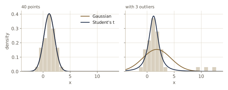
The same construction works in \(D\) dimensions: mixing \(\mathcal{N}(\mathbf{x} \mid \boldsymbol{\mu}, (\eta\boldsymbol{\Lambda})^{-1})\) over \(\eta \sim \operatorname{Gam}(\nu/2, \nu/2)\) gives the multivariate t-distribution
\[\operatorname{St}(\mathbf{x} \mid \boldsymbol{\mu}, \boldsymbol{\Lambda}, \nu) = \frac{\Gamma(D/2 + \nu/2)}{\Gamma(\nu/2)} \frac{\lvert \boldsymbol{\Lambda} \rvert^{1/2}}{(\pi\nu)^{D/2}} \Bigl[ 1 + \frac{\Delta^2}{\nu} \Bigr]^{-D/2 - \nu/2},\]where \(\Delta^2 = (\mathbf{x} - \boldsymbol{\mu})^{\mathrm{T}} \boldsymbol{\Lambda} (\mathbf{x} - \boldsymbol{\mu})\) is the squared Mahalanobis distance. It has mean \(\boldsymbol{\mu}\) (for \(\nu > 1\)), covariance \(\frac{\nu}{\nu - 2}\boldsymbol{\Lambda}^{-1}\) (for \(\nu > 2\)), and mode \(\boldsymbol{\mu}\).
Periodic variables
Some quantities live on a circle: wind direction, the hour of the day, the phase of a cycle. Represent one by an angle \(\theta \in [0, 2\pi)\). A Gaussian on \(\theta\) is a poor model, because the answer then depends on where we put the zero of the angle. Even the average goes wrong: five wind directions clustered around north give a naive average that points almost the opposite way.
deg = np.array([350.0, 355.0, 5.0, 10.0, 20.0])     # compass directions near north
theta = np.deg2rad(deg)
circ = np.rad2deg(np.arctan2(np.sin(theta).sum(), np.cos(theta).sum())) % 360
print(f"naive average: {deg.mean():.1f} deg;  circular mean: {circ:.1f} deg")
shifted = (deg + 180) % 360                          # same data, zero moved south
print(f"naive average with the zero moved by 180 deg: "
      f"{(shifted.mean() - 180) % 360:.1f} deg")
naive average: 148.0 deg;  circular mean: 4.0 deg
naive average with the zero moved by 180 deg: 4.0 deg
The fix is to treat each angle as a point on the unit circle, \(\mathbf{x}_n = (\cos\theta_n, \sin\theta_n)\), average those vectors, and take the angle of the average:
\[\bar{\theta} = \operatorname{atan2}\Bigl( \sum_n \sin\theta_n, \ \sum_n \cos\theta_n \Bigr),\]where \(\operatorname{atan2}\) is the two-argument arctangent that returns the angle in the correct quadrant. This does not depend on the choice of origin. The length \(\bar{r}\) of the average vector (between 0 and 1) measures how concentrated the angles are.
A Gaussian-like density on the circle arises from a two-dimensional isotropic Gaussian with mean at polar coordinates \((r_0, \theta_0)\) and variance \(\sigma^2\), restricted to the unit circle. Writing \(\mathbf{x} = (\cos\theta, \sin\theta)\) in the exponent and using \(\cos^2 + \sin^2 = 1\) and \(\cos A\cos B + \sin A\sin B = \cos(A - B)\), everything except a term \(\frac{r_0}{\sigma^2}\cos(\theta - \theta_0)\) is constant in \(\theta\). Normalizing gives the von Mises distribution
\[p(\theta \mid \theta_0, m) = \frac{1}{2\pi I_0(m)} \exp\{ m \cos(\theta - \theta_0) \},\]with mean direction \(\theta_0\) and concentration \(m = r_0/\sigma^2\), which plays the role of a precision. The normalizer involves \(I_0(m) = \frac{1}{2\pi} \int_0^{2\pi} \exp\{m\cos\theta\} \, d\theta\), the modified Bessel function of the first kind of order zero. For large \(m\) it is close to a Gaussian in \(\theta\) with variance \(1/m\). Maximizing the log-likelihood \(m\sum_n \cos(\theta_n - \theta_0) - N\ln(2\pi I_0(m))\) over \(\theta_0\) gives exactly the circular mean \(\bar{\theta}\) above. Over \(m\) it gives the equation \(A(m) = \bar{r}\), where \(A(m) = I_1(m)/I_0(m)\) increases from 0 to 1, so it can be solved numerically, here by bisection. SciPy’s i0e and i1e compute \(e^{-m}I_0(m)\) and \(e^{-m}I_1(m)\), which avoids overflow for large \(m\).
def von_mises_logpdf(theta, theta0, m):
    """ln p(theta | theta0, m); since i0e(m) = exp(-m) I0(m), ln I0(m) = ln i0e(m) + m."""
    return m * np.cos(theta - theta0) - np.log(2 * np.pi * i0e(m)) - m

def fit_von_mises(theta):
    """ML estimates: theta0 is the circular mean; m solves I1(m)/I0(m) = rbar,
    found by bisection on a log scale."""
    S, C = np.sin(theta).sum(), np.cos(theta).sum()
    rbar = np.hypot(S, C) / len(theta)
    lo, hi = 1e-8, 1e4
    for _ in range(100):
        mid = np.sqrt(lo * hi)
        lo, hi = (mid, hi) if i1e(mid) / i0e(mid) < rbar else (lo, mid)
    return np.arctan2(S, C), np.sqrt(lo * hi)

rng_vm = np.random.default_rng(17)
sample = rng_vm.vonmises(np.deg2rad(350), 4.0, size=500)
t0, m_hat = fit_von_mises(sample)
print(f"theta0_ML = {np.rad2deg(t0) % 360:.1f} deg, m_ML = {m_hat:.3f}  (true: 350 deg, 4)")
g = np.linspace(-np.pi, np.pi, 100_001)
area = np.trapezoid(np.exp(von_mises_logpdf(g, t0, m_hat)), g)
print(f"density integrates to {area:.6f}")
ref = stats.vonmises.logpdf(g[::5000], m_hat, loc=t0)
print("matches scipy:", np.allclose(von_mises_logpdf(g[::5000], t0, m_hat), ref))
theta0_ML = 348.7 deg, m_ML = 4.043  (true: 350 deg, 4)
density integrates to 1.000000
matches scipy: True
Other routes to periodic densities exist: histograms of the angle, “wrapping” a density on the real line around the circle, or marginalizing (rather than conditioning) a 2-D Gaussian onto the circle. The von Mises is the simplest to work with. It has a single peak, but mixtures of von Mises distributions handle several (Bishop §2.3.8 and Mardia and Jupp’s book on directional statistics go further).
Mixtures of Gaussians
A single Gaussian cannot model data that fall into two clumps; it puts its peak in the empty space between them. A mixture of Gaussians combines \(K\) of them:
\[p(\mathbf{x}) = \sum_{k=1}^{K} \pi_k \, \mathcal{N}(\mathbf{x} \mid \boldsymbol{\mu}_k, \boldsymbol{\Sigma}_k).\]Each Gaussian is a component with its own mean and covariance, and the weights \(\pi_k\) are mixing coefficients. Integrating both sides over \(\mathbf{x}\) shows \(\sum_k \pi_k = 1\), and requiring \(p(\mathbf{x}) \ge 0\) everywhere forces \(\pi_k \ge 0\) (look far out, where one component dominates). So the \(\pi_k\) are probabilities, and the mixture has a generative reading: pick component \(k\) with probability \(p(k) = \pi_k\), then draw \(\mathbf{x}\) from \(p(\mathbf{x} \mid k) = \mathcal{N}(\mathbf{x} \mid \boldsymbol{\mu}_k, \boldsymbol{\Sigma}_k)\). With enough components, a Gaussian mixture can approximate essentially any continuous density.
Bayes’ theorem then gives the probability that a given point came from component \(k\), called its responsibility:
\[\gamma_k(\mathbf{x}) = p(k \mid \mathbf{x}) = \frac{\pi_k \, \mathcal{N}(\mathbf{x} \mid \boldsymbol{\mu}_k, \boldsymbol{\Sigma}_k)}{\sum_{j} \pi_j \, \mathcal{N}(\mathbf{x} \mid \boldsymbol{\mu}_j, \boldsymbol{\Sigma}_j)}.\]The log-likelihood of a data set is
\[\ln p(\mathbf{X} \mid \boldsymbol{\pi}, \boldsymbol{\mu}, \boldsymbol{\Sigma}) = \sum_{n=1}^{N} \ln \Bigl\{ \sum_{k=1}^{K} \pi_k \, \mathcal{N}(\mathbf{x}_n \mid \boldsymbol{\mu}_k, \boldsymbol{\Sigma}_k) \Bigr\}.\]The sum over components sits inside the logarithm, so the log no longer turns the Gaussian into a quadratic, and setting derivatives to zero gives coupled equations with no closed-form solution. One can maximize with a general-purpose optimizer, but the standard tool is the EM algorithm of module 09. Here we build the pieces that module will use: the log-density (with log-sum-exp, since the component densities can underflow), the responsibilities, and an ancestral sampler.
def gmm_logpdf(X, pis, mus, Sigmas):
    """ln sum_k pi_k N(x | mu_k, Sigma_k) for each row of X, and the component terms."""
    logs = np.stack([np.log(p) + gaussian_logpdf(X, m, S)
                     for p, m, S in zip(pis, mus, Sigmas)], axis=1)
    return logsumexp(logs, axis=1), logs

def gmm_responsibilities(X, pis, mus, Sigmas):
    total, logs = gmm_logpdf(X, pis, mus, Sigmas)
    return np.exp(logs - total[:, None])

def gmm_sample(pis, mus, Sigmas, size, rng):
    """Ancestral sampling: pick component k with probability pi_k, then draw from it."""
    k = rng.choice(len(pis), size=size, p=pis)
    X = np.empty((size, len(mus[0])))
    for j in range(len(pis)):
        X[k == j] = gaussian_sample(mus[j], Sigmas[j], np.sum(k == j), rng)
    return X, k

pis = np.array([0.5, 0.3, 0.2])
mus_g = [np.array([0.0, 0.0]), np.array([3.0, 1.0]), np.array([1.0, 3.0])]
Sigmas_g = [np.array([[1.0, 0.5], [0.5, 1.0]]), 0.5 * np.eye(2),
            np.array([[0.3, 0.0], [0.0, 1.0]])]
rng_gmm = np.random.default_rng(19)
Xg, kg = gmm_sample(pis, mus_g, Sigmas_g, 1000, rng_gmm)

u = np.linspace(-6, 8, 561)
G1, G2 = np.meshgrid(u, u)
grid2 = np.column_stack([G1.ravel(), G2.ravel()])
dens = np.exp(gmm_logpdf(grid2, pis, mus_g, Sigmas_g)[0])
print(f"mixture density integrates to {dens.sum() * (u[1] - u[0])**2:.4f} on a grid")
three = np.array([[0.0, 0.0], [2.0, 1.5], [1.0, 3.0]])
print("responsibilities of three points:\n",
      gmm_responsibilities(three, pis, mus_g, Sigmas_g))
mu1, S1 = gaussian_ml(Xg)
print(f"average log-likelihood: one Gaussian fit by ML "
      f"{gaussian_logpdf(Xg, mu1, S1).mean():.4f}; "
      f"the true mixture {gmm_logpdf(Xg, pis, mus_g, Sigmas_g)[0].mean():.4f}")
mixture density integrates to 1.0000 on a grid
responsibilities of three points:
 [[0.9986 0.     0.0013]
 [0.254  0.6601 0.086 ]
 [0.0146 0.0005 0.9848]]
average log-likelihood: one Gaussian fit by ML -3.5967; the true mixture -3.2696
A point halfway between two components gets split responsibility, while a point at a component’s center belongs mostly to it. Even the best single Gaussian gives the data a clearly lower likelihood than the mixture that generated them.
The exponential family
Natural parameters
Almost every distribution in this module, the mixture excepted, is a member of one family. The exponential family consists of distributions of the form
\[p(\mathbf{x} \mid \boldsymbol{\eta}) = h(\mathbf{x}) \, g(\boldsymbol{\eta}) \exp\{ \boldsymbol{\eta}^{\mathrm{T}} \mathbf{u}(\mathbf{x}) \},\]where \(\boldsymbol{\eta}\) are the natural parameters, \(\mathbf{u}(\mathbf{x})\) is a vector of functions of the data, \(h(\mathbf{x})\) is a base measure, and \(g(\boldsymbol{\eta})\) is the normalizer, chosen so that \(g(\boldsymbol{\eta}) \int h(\mathbf{x}) \exp\{\boldsymbol{\eta}^{\mathrm{T}}\mathbf{u}(\mathbf{x})\} \, d\mathbf{x} = 1\) (a sum for discrete \(\mathbf{x}\)). The variable may be discrete or continuous, scalar or vector.
Bernoulli. Write the density as the exponential of its logarithm: \(\mu^x(1 - \mu)^{1-x} = (1 - \mu)\exp\{x \ln\frac{\mu}{1 - \mu}\}\). So \(\eta = \ln\frac{\mu}{1 - \mu}\), the log-odds, and solving for \(\mu\) gives \(\mu = \sigma(\eta) = 1/(1 + e^{-\eta})\), the logistic sigmoid. Since \(1 - \sigma(\eta) = \sigma(-\eta)\),
\[p(x \mid \eta) = \sigma(-\eta) \exp(\eta x), \qquad u(x) = x, \quad h(x) = 1, \quad g(\eta) = \sigma(-\eta).\]Multinomial (one observation, 1-of-K). \(\prod_k \mu_k^{x_k} = \exp\{\sum_k x_k \ln\mu_k\}\), so \(\eta_k = \ln\mu_k\) with \(u = \mathbf{x}\), \(h = 1\), \(g = 1\). These \(K\) natural parameters are not free, since the \(\mu_k\) must sum to one. To remove the constraint, eliminate \(\mu_K = 1 - \sum_{k<K}\mu_k\) and use the \(K - 1\) parameters \(\eta_k = \ln(\mu_k/\mu_K)\). Inverting gives the softmax (normalized exponential)
\[\mu_k = \frac{\exp(\eta_k)}{1 + \sum_{j=1}^{K-1} \exp(\eta_j)}, \qquad p(\mathbf{x} \mid \boldsymbol{\eta}) = \Bigl( 1 + \sum_{k=1}^{K-1} \exp(\eta_k) \Bigr)^{-1} \exp(\boldsymbol{\eta}^{\mathrm{T}}\mathbf{x}),\]where now \(\boldsymbol{\eta}\) and \(\mathbf{x}\) have their first \(K - 1\) entries only. The sigmoid and the softmax reappear in module 04, where logistic regression uses them to turn a linear function of the input into class probabilities; this is where they come from.
Gaussian. Expanding the square in the exponent, \(-\frac{1}{2\sigma^2}(x - \mu)^2 = \frac{\mu}{\sigma^2}x - \frac{1}{2\sigma^2}x^2 - \frac{\mu^2}{2\sigma^2}\), so
\[\boldsymbol{\eta} = \begin{pmatrix} \mu/\sigma^2 \\ -1/(2\sigma^2) \end{pmatrix}, \qquad \mathbf{u}(x) = \begin{pmatrix} x \\ x^2 \end{pmatrix},\] \[h(x) = (2\pi)^{-1/2}, \qquad g(\boldsymbol{\eta}) = (-2\eta_2)^{1/2} \exp\Bigl( \frac{\eta_1^2}{4\eta_2} \Bigr).\]We check all three natural forms against the ordinary formulas.
mu_b = 0.3
eta_b = np.log(mu_b / (1 - mu_b))
print(f"Bernoulli: eta = {eta_b:.4f}, sigma(eta) = {expit(eta_b):.4f};"
      f" p(1) = {expit(-eta_b) * np.exp(eta_b):.4f}, p(0) = {expit(-eta_b):.4f}")

mu_m = np.array([0.2, 0.5, 0.3])
eta_m = np.log(mu_m[:-1] / mu_m[-1])             # K - 1 free natural parameters
g_m = 1 / (1 + np.exp(eta_m).sum())
probs = [g_m * np.exp(eta_m @ xk[:-1]) for xk in np.eye(3)]
print("multinomial: probabilities from the natural form", np.array(probs))

mu_g, s2_g = 1.5, 0.8
eta_g = np.array([mu_g / s2_g, -1 / (2 * s2_g)])
def gauss_natural(x, eta):
    g = np.sqrt(-2 * eta[1]) * np.exp(eta[0]**2 / (4 * eta[1]))
    return (2 * np.pi)**-0.5 * g * np.exp(eta[0] * x + eta[1] * x**2)
xt = np.array([-1.0, 0.5, 2.0])
usual = np.exp(gaussian_logpdf(xt[:, None], np.array([mu_g]), np.array([[s2_g]])))
print("Gaussian: natural form", gauss_natural(xt, eta_g), " usual form", usual)
Bernoulli: eta = -0.8473, sigma(eta) = 0.3000; p(1) = 0.3000, p(0) = 0.7000
multinomial: probabilities from the natural form [0.2 0.5 0.3]
Gaussian: natural form [0.009  0.2387 0.3815]  usual form [0.009  0.2387 0.3815]
Maximum likelihood and sufficient statistics
The normalizer holds a surprising amount of information. Differentiate the normalization condition \(g(\boldsymbol{\eta}) \int h(\mathbf{x}) \exp\{\boldsymbol{\eta}^{\mathrm{T}}\mathbf{u}(\mathbf{x})\} d\mathbf{x} = 1\) with respect to \(\boldsymbol{\eta}\):
\[\nabla g(\boldsymbol{\eta}) \int h(\mathbf{x}) e^{\boldsymbol{\eta}^{\mathrm{T}}\mathbf{u}(\mathbf{x})} d\mathbf{x} + g(\boldsymbol{\eta}) \int h(\mathbf{x}) e^{\boldsymbol{\eta}^{\mathrm{T}}\mathbf{u}(\mathbf{x})} \mathbf{u}(\mathbf{x}) \, d\mathbf{x} = \mathbf{0}.\]The first integral is \(1/g(\boldsymbol{\eta})\) and the second term is \(\mathbb{E}[\mathbf{u}(\mathbf{x})]\), so
\[-\nabla \ln g(\boldsymbol{\eta}) = \mathbb{E}[\mathbf{u}(\mathbf{x})].\]Differentiating again gives the covariance: \(-\nabla\nabla\ln g(\boldsymbol{\eta}) = \operatorname{cov}[\mathbf{u}(\mathbf{x})]\) (Bishop’s exercise 2.58). Moments come from derivatives, with no integration.
Now the likelihood of \(N\) i.i.d. points is \(\bigl(\prod_n h(\mathbf{x}_n)\bigr) g(\boldsymbol{\eta})^N \exp\{\boldsymbol{\eta}^{\mathrm{T}}\sum_n\mathbf{u}(\mathbf{x}_n)\}\). Setting the gradient of its log to zero gives
\[-\nabla \ln g(\boldsymbol{\eta}_{\mathrm{ML}}) = \frac{1}{N} \sum_{n=1}^{N} \mathbf{u}(\mathbf{x}_n).\]Two consequences. First, the data enter only through \(\sum_n \mathbf{u}(\mathbf{x}_n)\), which is therefore the sufficient statistic: to fit the model we can throw away the data and keep that sum and the count \(N\). For the Bernoulli this is the number of heads; for the Gaussian, \(\sum_n x_n\) and \(\sum_n x_n^2\). Second, combined with the previous identity, the ML condition says: choose the parameters so that the model’s expected sufficient statistics equal their averages in the data. This is moment matching. As \(N \to \infty\) the data average tends to the true expectation, so \(\boldsymbol{\eta}_{\mathrm{ML}}\) tends to the true value.
def neg_log_g_gauss(eta):
    """-ln g(eta) for the univariate Gaussian in natural form."""
    return -(0.5 * np.log(-2 * eta[1]) + eta[0]**2 / (4 * eta[1]))

h = 1e-6
grad = np.array([(neg_log_g_gauss(eta_g + h * e) - neg_log_g_gauss(eta_g - h * e))
                 / (2 * h) for e in np.eye(2)])          # central differences
print("-grad ln g(eta) =", grad,
      "  E[u(x)] = (mu, mu^2 + sigma^2) =", np.array([mu_g, mu_g**2 + s2_g]))

# ML from sufficient statistics accumulated in chunks, as if the data streamed past
stream = rng.normal(mu_g, np.sqrt(s2_g), size=100_000)
N_seen, sum_x, sum_x2 = 0, 0.0, 0.0
for chunk in np.array_split(stream, 10):
    N_seen += len(chunk)
    sum_x += chunk.sum()
    sum_x2 += np.sum(chunk**2)
m1, m2 = sum_x / N_seen, sum_x2 / N_seen          # data averages of u(x) = (x, x^2)
print(f"moment matching: mu = {m1:.4f}, sigma^2 = {m2 - m1**2:.4f};  "
      f"batch ML: {stream.mean():.4f}, {stream.var():.4f}")
-grad ln g(eta) = [1.5  3.05]   E[u(x)] = (mu, mu^2 + sigma^2) = [1.5  3.05]
moment matching: mu = 1.4978, sigma^2 = 0.8010;  batch ML: 1.4978, 0.8010
Conjugate priors
Every member of the exponential family has a conjugate prior, and it has a standard form:
\[p(\boldsymbol{\eta} \mid \boldsymbol{\chi}, \nu) = f(\boldsymbol{\chi}, \nu) \, g(\boldsymbol{\eta})^{\nu} \exp\{ \nu \, \boldsymbol{\eta}^{\mathrm{T}} \boldsymbol{\chi} \},\]with \(f\) the normalizer. Multiplying by the likelihood,
\[p(\boldsymbol{\eta} \mid \mathbf{X}, \boldsymbol{\chi}, \nu) \propto g(\boldsymbol{\eta})^{\nu + N} \exp\Bigl\{ \boldsymbol{\eta}^{\mathrm{T}} \Bigl( \nu\boldsymbol{\chi} + \sum_{n=1}^{N} \mathbf{u}(\mathbf{x}_n) \Bigr) \Bigr\},\]which has the same form with \(\nu \to \nu + N\) and \(\nu\boldsymbol{\chi} \to \nu\boldsymbol{\chi} + \sum_n \mathbf{u}(\mathbf{x}_n)\). This explains the pseudo-count readings we kept finding: the prior behaves like \(\nu\) earlier observations whose average sufficient statistic was \(\boldsymbol{\chi}\).
For the Bernoulli, \(g(\eta)^\nu e^{\nu\chi\eta} = (1 - \mu)^{\nu}\bigl(\frac{\mu}{1 - \mu}\bigr)^{\nu\chi} = \mu^{\nu\chi}(1 - \mu)^{\nu(1 - \chi)}\). This is a density over \(\eta\). Converting it to a density over \(\mu\) multiplies by \(\lvert d\eta/d\mu \rvert = 1/(\mu(1 - \mu))\), which gives \(\mu^{\nu\chi - 1}(1 - \mu)^{\nu(1-\chi) - 1}\): the beta distribution with \(a = \nu\chi\) and \(b = \nu(1 - \chi)\). So \(\nu = a + b\) is the number of pseudo-flips and \(\chi = a/(a + b)\) is their fraction of heads.
nu_c, chi_c = 6.0, 0.25                     # six pseudo-flips, a quarter of them heads
mus_c = np.array([0.1, 0.3, 0.5, 0.8])
etas_c = np.log(mus_c / (1 - mus_c))
# ln of g(eta)^nu exp(nu chi eta), unnormalized
log_prior_eta = nu_c * np.log(expit(-etas_c)) + nu_c * chi_c * etas_c
log_prior_mu = log_prior_eta - np.log(mus_c * (1 - mus_c))   # change of variables to mu
print("log density minus ln Beta(mu | nu chi, nu (1 - chi)):",
      log_prior_mu - beta_logpdf(mus_c, nu_c * chi_c, nu_c * (1 - chi_c)))
log density minus ln Beta(mu | nu chi, nu (1 - chi)): [-2.4545 -2.4545 -2.4545 -2.4545]
The difference is the same at every \(\mu\) (it is the log of the normalizer we left out), so the two densities agree up to normalization.
Noninformative priors
Sometimes we want a prior that says as little as possible, a noninformative prior. The obvious candidate, a constant, has two problems for continuous parameters. If the parameter ranges over an unbounded set, a constant density cannot be normalized; such a prior is called improper. Improper priors are often usable anyway, as long as the posterior they produce is proper: a flat prior on a Gaussian’s mean gives a proper posterior after a single observation, and it is the \(\sigma_0^2 \to \infty\) limit we took earlier.
The second problem is that “flat” depends on the parameterization. A density that is constant in \(\lambda\) is not constant in \(\eta\) if \(\lambda = \eta^2\), because densities pick up the Jacobian factor \(\lvert d\lambda/d\eta \rvert\) when variables change. Maximum likelihood does not care about this (the maximizer of a function does not move when we relabel the axis), but a prior does. For instance, a uniform prior on a coin’s \(\mu\) is far from uniform on the log-odds scale:
mu_u = rng.random(1_000_000)                  # uniform prior on mu
eta_u = np.log(mu_u / (1 - mu_u))             # the same prior on the log-odds scale
low, high = np.mean((eta_u > 0) & (eta_u < 1)), np.mean((eta_u > 4) & (eta_u < 5))
print(f"P(0 < eta < 1) = {low:.4f},  P(4 < eta < 5) = {high:.4f}")
P(0 < eta < 1) = 0.2315, P(4 < eta < 5) = 0.0114
On the log-odds scale the “flat” prior puts twenty times more mass between 0 and 1 than between 4 and 5.
Invariance arguments pick out sensible choices in two common cases. If a density has the form \(p(x \mid \mu) = f(x - \mu)\), then \(\mu\) is a location parameter, and shifting \(x\) just shifts \(\mu\); asking the prior to give equal mass to an interval and to any shifted copy of it forces \(p(\mu)\) to be constant. If \(p(x \mid \sigma) = \frac{1}{\sigma}f(x/\sigma)\) with \(\sigma > 0\), then \(\sigma\) is a scale parameter; asking for equal mass on \([A, B]\) and on \([A/c, B/c]\) for every \(c > 0\) forces \(p(\sigma) \propto 1/\sigma\), which is flat in \(\ln\sigma\) (as much prior mass between 1 and 10 as between 10 and 100). For a Gaussian, the mean is a location parameter and the standard deviation a scale parameter. In terms of the precision, \(p(\sigma) \propto 1/\sigma\) becomes \(p(\lambda) \propto 1/\lambda\), the \(a_0 = b_0 = 0\) limit of the gamma prior, and indeed with \(a_0 = b_0 = 0\) the posterior parameters \(a_N\), \(b_N\) above depend only on the data. Both invariant priors are improper.
Nonparametric methods
Histograms
A parametric model fixes the shape of the density in advance, and if the shape is wrong, no amount of data will fix it: a Gaussian stays unimodal however many bimodal points we give it. Nonparametric methods let the data determine the shape. (They still have parameters, but those control smoothness rather than form.) We use one-dimensional data from a two-component mixture throughout, so we can compare every estimate with the truth.
The simplest estimate is a histogram: split the line into bins of width \(\Delta_i\), count the \(n_i\) points in bin \(i\), and set the density in that bin to
\[p_i = \frac{n_i}{N \Delta_i},\]which integrates to one. The bin width is a smoothing parameter. Very narrow bins give a spiky estimate that is zero in every empty bin; very wide bins blur the two modes into one. Because we know the true density \(p\) here, we can score an estimate \(\hat{p}\) directly by its integrated squared error \(\int (\hat{p}(x) - p(x))^2 \, dx\), computed on a fine grid. With real data the truth is unknown, and we would score an estimate by its average log-likelihood on a separate validation set instead, the device module 01 used to choose a polynomial degree. A histogram makes that awkward, as the second column shows: a validation point in an empty bin has probability zero and log-likelihood \(-\infty\).
def normal_pdf(x, m, s2):
    return np.exp(-(x - m)**2 / (2 * s2)) / np.sqrt(2 * np.pi * s2)

def true_density(x):
    return 0.35 * normal_pdf(x, 0.25, 0.08**2) + 0.65 * normal_pdf(x, 0.65, 0.1**2)

def sample_true(n, rng):
    first = rng.random(n) < 0.35
    return np.where(first, rng.normal(0.25, 0.08, n), rng.normal(0.65, 0.1, n))

rng_np = np.random.default_rng(23)
x_tr = sample_true(60, rng_np)                  # training points
x_va = sample_true(2000, rng_np)                # validation points

gx = np.linspace(-0.5, 1.5, 4001)          # grid for comparing estimates with the truth

def ise(p_hat):
    """Integrated squared error of an estimate given on the grid gx."""
    return np.trapezoid((p_hat - true_density(gx))**2, gx)

def hist_density(x, x_train, width, lo=-0.5, hi=1.5):
    """Histogram estimate n_i / (N width) at the points x; equal bins from lo to hi."""
    edges = np.arange(lo, hi + width / 2, width)
    counts, _ = np.histogram(x_train, bins=edges)
    p = counts / (len(x_train) * width)
    return p[np.clip(np.searchsorted(edges, x, side="right") - 1, 0, len(p) - 1)]

for width in (0.02, 0.05, 0.1, 0.25, 0.5):
    empty = np.mean(hist_density(x_va, x_tr, width) == 0)
    err = ise(hist_density(gx, x_tr, width))
    print(f"bin width {width:4.2f}: integrated squared error {err:.3f}, "
          f"validation points in empty bins {empty:6.1%}")
bin width 0.02: integrated squared error 0.944, validation points in empty bins  27.6%
bin width 0.05: integrated squared error 0.427, validation points in empty bins  11.2%
bin width 0.10: integrated squared error 0.219, validation points in empty bins   9.8%
bin width 0.25: integrated squared error 0.294, validation points in empty bins   0.1%
bin width 0.50: integrated squared error 0.601, validation points in empty bins   0.1%
The error is smallest for bins of width 0.1 and grows in both directions. With the narrowest bins, more than a quarter of the validation points (27.6%) land in bins that received no training point, where the histogram says they cannot occur. The widest bins have almost no empty bins but lose the two-peaked shape.
Histograms have practical merits: once the counts are made, the data can be discarded, and new points can be added as they arrive. But the estimate jumps at bin edges for no reason that has to do with the data, and in \(D\) dimensions, \(M\) bins per axis means \(M^D\) bins in all, most of them empty unless \(N\) is astronomically large. That is the curse of dimensionality from module 01. The histogram teaches two lessons that carry over: to estimate the density at a point, look at the data in a neighborhood of it; and the size of that neighborhood must be neither too small nor too large.
Kernel density estimators
Make the neighborhood idea precise. Let \(\mathcal{R}\) be a small region around \(\mathbf{x}\) with volume \(V\), and let \(P = \int_{\mathcal{R}} p(\mathbf{x}') \, d\mathbf{x}'\) be its probability. Each of the \(N\) points falls in \(\mathcal{R}\) with probability \(P\), so the count \(K\) is binomial, \(\operatorname{Bin}(K \mid N, P)\), with \(\mathbb{E}[K/N] = P\) and \(\operatorname{var}[K/N] = P(1 - P)/N\). For large \(N\), then, \(K \approx NP\). If \(\mathcal{R}\) is also small enough that \(p\) is nearly constant on it, \(P \approx p(\mathbf{x})V\). Together,
\[p(\mathbf{x}) \approx \frac{K}{NV}.\]The two assumptions pull in opposite directions (the region must be small for \(p\) to be constant, but must hold enough points for \(K/N\) to be reliable), which is the smoothing trade-off again. We can use the formula in two ways: fix \(V\) and count \(K\), or fix \(K\) and find \(V\). Both converge to the true density as \(N \to \infty\), provided \(V\) shrinks and \(K\) grows at suitable rates.
Fixing \(V\): take \(\mathcal{R}\) to be a cube of side \(h\) centered at \(\mathbf{x}\). With \(k(\mathbf{u}) = 1\) if every \(\lvert u_i \rvert \le \frac{1}{2}\) and 0 otherwise (a Parzen window), the count is \(K = \sum_n k((\mathbf{x} - \mathbf{x}_n)/h)\) and
\[p(\mathbf{x}) = \frac{1}{N} \sum_{n=1}^{N} \frac{1}{h^D} k\Bigl( \frac{\mathbf{x} - \mathbf{x}_n}{h} \Bigr).\]Read the other way, this puts a small cube of mass \(1/N\) on each data point and adds them up. Cubes have edges, so the estimate still jumps. Any kernel \(k(\mathbf{u}) \ge 0\) with \(\int k(\mathbf{u}) \, d\mathbf{u} = 1\) gives a valid density, and a smooth kernel gives a smooth estimate. The usual choice is Gaussian:
\[p(\mathbf{x}) = \frac{1}{N} \sum_{n=1}^{N} \frac{1}{(2\pi h^2)^{D/2}} \exp\Bigl\{ -\frac{\lVert \mathbf{x} - \mathbf{x}_n \rVert^2}{2h^2} \Bigr\},\]a kernel density estimator (or Parzen estimator) with bandwidth \(h\). We compute it in log space so that points far from all the data get a very negative log density instead of an underflow to zero.
def kde_logpdf(Xq, Xtr, h):
    """ln of the Gaussian kernel density estimate (bandwidth h) at each query row."""
    Xq, Xtr = Xq.reshape(len(Xq), -1), Xtr.reshape(len(Xtr), -1)
    D = Xtr.shape[1]
    d2 = ((Xq[:, None, :] - Xtr[None, :, :])**2).sum(axis=2)
    return (logsumexp(-d2 / (2 * h**2), axis=1) - np.log(len(Xtr))
            - 0.5 * D * np.log(2 * np.pi * h**2))

g = np.linspace(-1.0, 2.0, 30001)
print(f"integrates to {np.trapezoid(np.exp(kde_logpdf(g, x_tr, 0.05)), g):.6f}")
ref = stats.norm.pdf(g[:5, None], x_tr, 0.05).mean(axis=1)
print("matches an average of scipy normal densities:",
      np.allclose(np.exp(kde_logpdf(g[:5], x_tr, 0.05)), ref))
for h in (0.005, 0.01, 0.02, 0.03, 0.05, 0.08, 0.15, 0.3):
    val = kde_logpdf(x_va, x_tr, h).mean()
    err = ise(np.exp(kde_logpdf(gx, x_tr, h)))
    print(f"h = {h:5.3f}: validation mean log-lik {val:6.3f}, "
          f"integrated squared error {err:.3f}")
print(f"true density: validation mean log-lik {np.log(true_density(x_va)).mean():.3f}")
integrates to 1.000000
matches an average of scipy normal densities: True
h = 0.005: validation mean log-lik -2.656, integrated squared error 1.065
h = 0.010: validation mean log-lik -0.377, integrated squared error 0.520
h = 0.020: validation mean log-lik  0.140, integrated squared error 0.218
h = 0.030: validation mean log-lik  0.238, integrated squared error 0.120
h = 0.050: validation mean log-lik  0.278, integrated squared error 0.074
h = 0.080: validation mean log-lik  0.252, integrated squared error 0.117
h = 0.150: validation mean log-lik  0.117, integrated squared error 0.318
h = 0.300: validation mean log-lik -0.115, integrated squared error 0.570
true density: validation mean log-lik 0.342
The validation log-likelihood rises and then falls as \(h\) grows, and it picks \(h = 0.05\), the same bandwidth that minimizes the integrated squared error (which we could compute only because we know the truth). A small bandwidth puts a spike on every training point and gives validation points between the spikes very low density; a large one smears the two modes together. At its best, the kernel estimate’s error, 0.074, is about a third of the best histogram’s, 0.219, from the same 60 points.
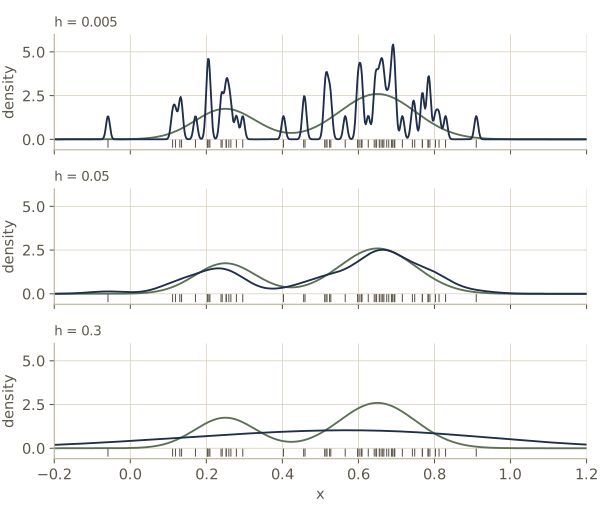
Kernel estimators need no training at all: “fitting” means storing the data. That is also their weakness. Every evaluation touches all \(N\) training points, so both memory and prediction time grow linearly with the size of the training set.
Nearest-neighbor density estimation
One bandwidth for the whole space is a compromise: in dense regions a wide kernel blurs detail, while in sparse regions a narrow one is noisy. The other way to use \(p \approx K/(NV)\) adapts automatically: fix \(K\), and let \(V\) be the volume of the smallest sphere around \(\mathbf{x}\) that contains \(K\) data points. In dense regions the sphere is small, in sparse regions large. This is K-nearest-neighbor (KNN) density estimation. In \(D\) dimensions a sphere of radius \(r\) has volume \(\frac{\pi^{D/2}}{\Gamma(D/2 + 1)}r^D\); in one dimension the “sphere” is an interval of length \(2r\).
def knn_density_1d(x_query, x_train, K):
    """K / (N V), V = length of the smallest interval around x holding K points."""
    dist = np.abs(x_query[:, None] - x_train[None, :])
    r = np.partition(dist, K - 1, axis=1)[:, K - 1]      # distance to the K-th neighbor
    return K / (len(x_train) * 2 * r)

for K in (5, 10, 15, 25, 40):
    p_grid = knn_density_1d(gx, x_tr, K)
    val = np.log(knn_density_1d(x_va, x_tr, K)).mean()
    print(f"K = {K:2d}: integrated squared error {ise(p_grid):.3f}, "
          f"area over the grid {np.trapezoid(p_grid, gx):.3f}, "
          f"validation mean log-lik {val:.3f}")
for Lim in (2, 20, 200, 2000):
    half = np.geomspace(1e-4, Lim, 20000)        # fine near 0.5, coarse far away
    xq = 0.5 + np.concatenate([-half[::-1], half])
    area = np.trapezoid(knn_density_1d(xq, x_tr, 5), xq)
    print(f"integral of the K = 5 estimate over [0.5 - {Lim}, 0.5 + {Lim}]: {area:.3f}")
K =  5: integrated squared error 0.886, area over the grid 1.504, validation mean log-lik 0.536
K = 10: integrated squared error 0.248, area over the grid 1.386, validation mean log-lik 0.422
K = 15: integrated squared error 0.273, area over the grid 1.456, validation mean log-lik 0.414
K = 25: integrated squared error 0.378, area over the grid 1.443, validation mean log-lik 0.286
K = 40: integrated squared error 0.546, area over the grid 1.405, validation mean log-lik 0.131
integral of the K = 5 estimate over [0.5 - 2, 0.5 + 2]: 1.580
integral of the K = 5 estimate over [0.5 - 20, 0.5 + 20]: 1.785
integral of the K = 5 estimate over [0.5 - 200, 0.5 + 200]: 1.978
integral of the K = 5 estimate over [0.5 - 2000, 0.5 + 2000]: 2.170
As with the bandwidth, \(K\) controls the smoothing: by integrated squared error, \(K = 10\) does best, and the error grows for smaller and larger \(K\). The validation log-likelihood tells a different story. It keeps improving as \(K\) shrinks, and at \(K = 5\) it even beats the true density’s score of 0.342, which is a warning sign. The area column explains it: the KNN estimate is not a proper density. Its area over \([-0.5, 1.5]\) is already around 1.4 to 1.5, so it hands out more density than it has, and log-likelihoods of unnormalized estimates cannot be compared. (With \(K = 1\) it is worse still: the estimate \(1/(2N\lvert x - x_n vert)\) near each training point has an infinite integral, so we left it out.) The second loop shows that the total area is not even finite. Far from the data the distance to the \(K\)-th neighbor grows only like \(\lvert x \rvert\), so the estimate decays like \(1/\lvert x \rvert\), whose integral diverges; the area keeps growing as the range widens, by about \((K/N)\ln 10 \approx 0.19\) for each factor of ten. KNN density estimates are still useful for comparing densities at points, which is exactly what the classifier below does.
The K-nearest-neighbor classifier
Nearest neighbors earn their keep in classification. Suppose the training set has \(N_k\) points in class \(\mathcal{C}_k\), \(N\) in all. To classify a new point \(\mathbf{x}\), draw the sphere around it that contains \(K\) training points of any class, with volume \(V\), and let \(K_k\) of them belong to class \(\mathcal{C}_k\). Then the density estimates are \(p(\mathbf{x} \mid \mathcal{C}_k) = K_k/(N_k V)\) for each class and \(p(\mathbf{x}) = K/(NV)\) overall, and the class priors are \(p(\mathcal{C}_k) = N_k/N\). Bayes’ theorem gives
\[p(\mathcal{C}_k \mid \mathbf{x}) = \frac{p(\mathbf{x} \mid \mathcal{C}_k) \, p(\mathcal{C}_k)}{p(\mathbf{x})} = \frac{K_k}{K}.\]To minimize the probability of misclassification (module 01’s decision rule), assign \(\mathbf{x}\) to the class with the most members among its \(K\) nearest neighbors. With \(K = 1\) this is the nearest-neighbor rule: copy the label of the closest training point. Its decision boundary is made of pieces of the perpendicular bisectors between nearby points of different classes. A classical result of Cover and Hart (1967) says that, as \(N \to \infty\), the nearest-neighbor rule makes at most twice as many errors as the best possible (Bayes-optimal) classifier.
We implement it with all pairwise squared distances computed at once, using \(\lVert \mathbf{a} - \mathbf{b} \rVert^2 = \lVert \mathbf{a} \rVert^2 + \lVert \mathbf{b} \rVert^2 - 2\mathbf{a}^{\mathrm{T}}\mathbf{b}\) (one matrix product instead of a three-dimensional array), and np.argpartition to find the \(K\) smallest in each row without sorting everything. The test data come from two classes that are each a pair of Gaussian blobs, so we also know the Bayes-optimal classifier and its error rate.
def knn_predict_proba(X_query, X_train, t_train, K, n_classes):
    """p(C_k | x) = K_k / K from the K nearest training points (Euclidean)."""
    d2 = (np.sum(X_query**2, axis=1)[:, None] + np.sum(X_train**2, axis=1)[None, :]
          - 2 * X_query @ X_train.T)
    nn = np.argpartition(d2, K - 1, axis=1)[:, :K]      # the K nearest, unordered
    votes = np.zeros((len(X_query), n_classes))
    np.add.at(votes, (np.arange(len(X_query))[:, None], t_train[nn]), 1)
    return votes / K

centers = [np.array([[-1.0, 0.0], [1.0, 1.5]]),           # class 0: two blobs
           np.array([[0.0, 1.0], [1.5, -0.5]])]           # class 1: two blobs
def make_two_class(n_per_class, rng):
    X, t = [], []
    for k, C in enumerate(centers):
        blob = C[rng.integers(0, 2, size=n_per_class)]      # one of the two blobs
        X.append(blob + 0.6 * rng.standard_normal((n_per_class, 2)))
        t.append(np.full(n_per_class, k))
    return np.vstack(X), np.concatenate(t)

rng_knn = np.random.default_rng(31)
X_tr, t_tr = make_two_class(100, rng_knn)
X_te, t_te = make_two_class(2000, rng_knn)

# brute-force check on 50 test points: sort all distances, vote among the first K
K = 5
brute = []
for q in X_te[:50]:
    nearest = np.argsort(np.sum((X_tr - q)**2, axis=1))[:K]
    brute.append(np.bincount(t_tr[nearest], minlength=2).argmax())
fast = knn_predict_proba(X_te[:50], X_tr, t_tr, K, 2).argmax(axis=1)
print("agrees with brute force:", np.array_equal(fast, brute))

def class_logpdf(X, C):
    """True class density: an equal mixture of two blobs with covariance 0.36 I."""
    comps = [gaussian_logpdf(X, c, 0.36 * np.eye(2)) for c in C]
    return logsumexp(comps, axis=0) - np.log(2)

bayes = (class_logpdf(X_te, centers[1]) > class_logpdf(X_te, centers[0])).astype(int)
print(f"Bayes-optimal test error: {np.mean(bayes != t_te):.3f}")
for K in (1, 3, 7, 15, 31, 61, 121):
    err = np.mean(knn_predict_proba(X_te, X_tr, t_tr, K, 2).argmax(axis=1) != t_te)
    print(f"K = {K:3d}: test error {err:.3f}")
agrees with brute force: True
Bayes-optimal test error: 0.171
K =   1: test error 0.228
K =   3: test error 0.194
K =   7: test error 0.187
K =  15: test error 0.180
K =  31: test error 0.180
K =  61: test error 0.180
K = 121: test error 0.464
With odd \(K\) and two classes there are no tied votes. The test error falls from 0.228 at \(K = 1\) to 0.180 for \(K\) between 15 and 61, close to the Bayes-optimal 0.171, then jumps to 0.464 at \(K = 121\), where every vote covers most of the 200 training points. (The nearest-neighbor rule’s 0.228 is well under twice the Bayes error, as the Cover–Hart bound leads us to expect, although that bound is a statement about infinite training sets.) Small \(K\) follows every quirk of the training sample; large \(K\) averages over so wide a neighborhood that it smooths away real structure, and at the extreme (\(K = N\)) it predicts the majority class everywhere.
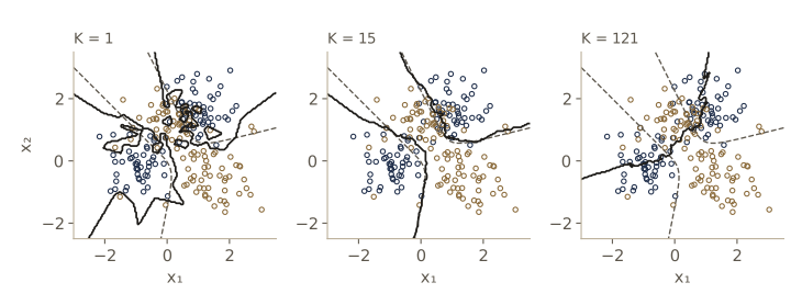
The price of all this flexibility is paid at prediction time. KNN, like the kernel estimator, stores the entire training set and compares each query with every stored point, so memory and prediction time both grow with \(N\).
import time
rng_t = np.random.default_rng(0)
Xq = rng_t.normal(size=(1000, 2))
for n_train in (2_000, 20_000):
    Xb, tb = make_two_class(n_train // 2, rng_t)
    t0 = time.perf_counter()
    knn_predict_proba(Xq, Xb, tb, 15, 2)
    ms = 1000 * (time.perf_counter() - t0)
    print(f"N = {n_train:6d}: {ms:7.1f} ms for 1000 queries (your times will differ); "
          f"stored numbers: {Xb.size}")
N =   2000:    18.0 ms for 1000 queries (your times will differ); stored numbers: 4000
N =  20000:   229.6 ms for 1000 queries (your times will differ); stored numbers: 40000
Watch out. A kernel density estimate or a KNN classifier has no compact summary of what it learned: the model is the training set. Memory grows with \(N\), and every prediction scans all \(N\) points. Tree-based search structures (k-d trees, ball trees) and approximate nearest-neighbor methods cut the search cost, at the price of extra preprocessing, but in high dimensions they help less than one hopes, and distances themselves become less informative.
Parametric models are compact but rigid; nonparametric models are flexible but grow with the data. Much of the rest of the course looks for models in between, whose flexibility we can control independently of \(N\): basis-function models (module 03), neural networks (module 05), sparse kernel machines (module 07), and mixtures (module 09).
Summary
| Model | Assumes | Fit by maximum likelihood | Conjugate prior and posterior |
|---|---|---|---|
| Bernoulli / binomial | binary outcomes, one probability \(\mu\) | \(\mu_{\mathrm{ML}} = m/N\) | \(\operatorname{Beta}(a, b) \to \operatorname{Beta}(a + m, b + l)\) |
| Multinomial (1-of-K) | \(K\) exclusive states, probabilities \(\mu_k\) | \(\mu_k = m_k/N\) (Lagrange multiplier) | \(\operatorname{Dir}(\boldsymbol{\alpha}) \to \operatorname{Dir}(\boldsymbol{\alpha} + \mathbf{m})\) |
| Gaussian, mean | known variance \(\sigma^2\) | sample mean | Gaussian; precisions add |
| Gaussian, precision | known mean | \(1/\sigma^2_{\mathrm{ML}}\) | \(\operatorname{Gam}(a_0 + N/2, \ b_0 + N\sigma^2_{\mathrm{ML}}/2)\) |
| Gaussian, both | unimodal, \(D(D+3)/2\) parameters | sample mean and covariance (biased by \((N-1)/N\)) | normal-gamma; normal-Wishart in \(D\) dimensions |
| Student’s t | Gaussian with gamma-distributed precision | iterative reweighting (EM) | (not conjugate) |
| von Mises | a direction on the circle | circular mean; solve \(A(m) = \bar{r}\) | (not covered here) |
| Gaussian mixture | \(K\) Gaussian components | no closed form; EM in module 09 | no closed-form posterior; approximated in module 10 |
| Exponential family | \(h(\mathbf{x})g(\boldsymbol{\eta})e^{\boldsymbol{\eta}^{\mathrm{T}}\mathbf{u}(\mathbf{x})}\) | moment matching: \(-\nabla\ln g =\) average of \(\mathbf{u}\) | \(g(\boldsymbol{\eta})^{\nu}e^{\nu\boldsymbol{\eta}^{\mathrm{T}}\boldsymbol{\chi}}\) |
| Histogram, kernel, KNN | only smoothness | store the data; choose bin width, \(h\), or \(K\) on validation data | (nonparametric) |
Ideas to carry forward:
- Maximum likelihood takes a small sample at face value and overfits it; a conjugate prior acts like extra pseudo-observations, and the posterior mean is a precision- or count-weighted compromise between prior and data that approaches the ML answer as \(N\) grows.
- For Gaussians, completing the square does everything: conditionals and marginals of a joint Gaussian are Gaussian, and the linear-Gaussian box turns \(p(\mathbf{x})\) and \(p(\mathbf{y} \mid \mathbf{x})\) into \(p(\mathbf{y})\) and \(p(\mathbf{x} \mid \mathbf{y})\). Modules 03, 06, 12, and 13 use it directly.
- Exponential-family models have sufficient statistics, fit by matching moments, and have conjugate priors; the sigmoid and softmax are their natural-parameter links.
- Nonparametric estimators trade a fixed shape for a smoothing parameter and a model that grows with the data; the smoothing parameter is chosen like any other complexity control, on held-out data.
Exercises
- Show that the mode of \(\operatorname{Beta}(\mu \mid a, b)\) is \((a - 1)/(a + b - 2)\) for \(a, b > 1\). The mode of the posterior is the maximum a posteriori (MAP) estimate. For the posterior after \(m\) heads and \(l\) tails, which prior makes the MAP estimate equal to \(\mu_{\mathrm{ML}}\)? Which makes it equal to Laplace’s rule \((m + 1)/(N + 2)\)?
- Using
bernoulli_loglik,beta_update, andpredictive_heads, simulate 10,000 experiments of \(N = 5\) flips of a coin with \(\mu = 0.2\). Compare the average log probability that the ML estimate and the Bayesian predictive distribution (with a Beta(1, 1) prior) assign to a sixth flip. Explain why ML sometimes scores \(-\infty\). - The variance identity in section 1 says the posterior is narrower than the prior on average. Find a beta prior and a data set of 10 flips for which the posterior variance is larger than the prior variance, and explain in words why this can happen.
- Prove that the multinomial log-likelihood \(\sum_k m_k \ln\mu_k\) is concave on the simplex, so the stationary point found with the Lagrange multiplier is the global maximum. Then compute the mean and variance of \(\mu_j\) under \(\operatorname{Dir}(\boldsymbol{\alpha})\) from the gamma-normalization sampler and compare with \(\alpha_j/\alpha_0\) and \(\alpha_j(\alpha_0 - \alpha_j)/(\alpha_0^2(\alpha_0 + 1))\).
- Show that the maximum likelihood fit of a Gaussian with diagonal covariance to data \(\mathbf{X}\) keeps the diagonal of \(\boldsymbol{\Sigma}_{\mathrm{ML}}\), and that the isotropic fit has \(\sigma^2 = \operatorname{tr}(\boldsymbol{\Sigma}_{\mathrm{ML}})/D\). Check both numerically by perturbing the solutions, as in the
gaussian_mlcell. - Verify the partitioned-inverse formula by multiplying the block matrix by its claimed inverse. Then use it to show that the precision \(\mathbf{R}\) of the linear-Gaussian joint has the inverse given in the text, and check your algebra numerically on a random example.
- Let \(\mathbf{x}_n \sim \mathcal{N}(\boldsymbol{\mu}, \boldsymbol{\Sigma})\) with \(\boldsymbol{\Sigma}\) known and prior \(\boldsymbol{\mu} \sim \mathcal{N}(\boldsymbol{\mu}_0, \boldsymbol{\Sigma}_0)\). Use the linear-Gaussian box, with \(\mathbf{y}\) the stacked data and \(\mathbf{A}\) a stack of \(N\) identity matrices, to derive the posterior over \(\boldsymbol{\mu}\). Simplify it so that it involves only \(N\) and the sample mean, and implement it for \(D = 2\).
- Show that \(\operatorname{St}(x \mid \mu, \lambda, \nu) \to \mathcal{N}(x \mid \mu, \lambda^{-1})\) as \(\nu \to \infty\). (Look only at the dependence on \(x\) and use \((1 + c/\nu)^{\nu} \to e^{c}\).) Confirm numerically with
student_t_logpdffor \(\nu = 10, 100, 1000\). - Derive the sequential update for the maximum likelihood variance of a univariate Gaussian with known mean, in the form \(\sigma^2_{(N)} = \sigma^2_{(N-1)} + a_{N-1}(\cdots)\), and show that it is a Robbins–Monro iteration on \(\partial \ln p(x \mid \sigma^2)/\partial\sigma^2\). What step sizes \(a_N\) make it exact?
- Write the beta, gamma, and von Mises distributions in exponential-family form, identifying \(\boldsymbol{\eta}\), \(\mathbf{u}(x)\), \(h(x)\), and \(g(\boldsymbol{\eta})\). For the gamma, verify \(-\nabla\ln g(\boldsymbol{\eta}) = \mathbb{E}[\mathbf{u}(x)]\) by finite differences.
- Extend
kde_logpdfto choose the bandwidth by 5-fold cross-validation on the training set alone (no separate validation set), and compare the chosen \(h\) with the one picked in the text. Then fit a two-dimensional KDE to the mixture sampleXgand compare its average log-likelihood on fresh samples with that of the true mixture. - In your own words: a friend says “nonparametric methods have no parameters, so they cannot overfit.” Explain what is wrong with this, using the histogram, the kernel estimator, and the KNN classifier from this module as examples.
Going further
- Bishop, Pattern Recognition and Machine Learning, chapter 2 and appendix B (a reference list of the distributions, with their moments). Exercises 2.7–2.8 (posterior means and variances), 2.24 and 2.29–2.33 (partitioned and linear-Gaussian results), 2.34–2.35 (the ML covariance and its bias), 2.38–2.40 (Bayesian inference for the mean), 2.44 (the normal-gamma posterior), 2.46–2.50 (Student’s t), 2.52–2.55 (von Mises), 2.56–2.58 (exponential family), and 2.60–2.61 (histograms and KNN) are all good practice after this module.
- Kevin P. Murphy, Probabilistic Machine Learning: An Introduction (MIT Press, 2022), freely available online — the early chapters on probability and statistics cover the same distributions and conjugate analysis from a slightly different angle, with many worked examples, and a later chapter on exemplar-based methods covers nearest neighbors and kernel density estimation.
- Herbert Robbins and Sutton Monro, “A stochastic approximation method”, Annals of Mathematical Statistics, 1951 — the paper behind sequential root finding and, eventually, stochastic gradient descent.
- Thomas M. Cover and Peter E. Hart, “Nearest neighbor pattern classification”, IEEE Transactions on Information Theory, 1967 — the factor-of-two bound on the nearest-neighbor error rate.
- B. W. Silverman, Density Estimation for Statistics and Data Analysis (Chapman and Hall, 1986) — a short, readable book on histograms and kernel estimators, including practical bandwidth selection.
- K. B. Petersen and M. S. Pedersen, The Matrix Cookbook — a free compendium of matrix identities, including the derivatives and partitioned inverses used in this module.
These notes follow the chapters of C. M. Bishop, Pattern Recognition and Machine Learning (Springer, 2006), the course text, which Microsoft Research makes freely available as a PDF. The explanations, code, figures, and exercises here are written for this course; the book remains the reference, with the full derivations and many more exercises.