CSE 474/574 · Module 12 · Week 13
Continuous Latent Variables
Principal component analysis two ways, probabilistic PCA and EM, factor analysis, kernel PCA, ICA, and autoencoders.
Companion reading: Bishop, Pattern Recognition and Machine Learning, chapter 12, “Continuous Latent Variables”
By the end of this module you can
- Derive principal component analysis both as the projection of maximum variance and as the projection of minimum squared reconstruction error, and show that the error equals the sum of the discarded eigenvalues.
- Use PCA for compression, reconstruction, whitening, and two-dimensional visualization, and compute it with the \(N \times N\) Gram-matrix trick when \(N < D\).
- Write down the probabilistic PCA model, derive its marginal \(p(\mathbf{x})\) and posterior \(p(\mathbf{z} \mid \mathbf{x})\), and derive its closed-form maximum likelihood solution.
- Implement EM for probabilistic PCA and for factor analysis, and explain when the two models give different answers.
- Explain how automatic relevance determination lets Bayesian PCA switch off unneeded columns of \(\mathbf{W}\).
- Derive kernel PCA from the centered Gram matrix, implement it with a Gaussian kernel, and project new points.
- Separate linearly mixed non-Gaussian sources with independent component analysis, and explain why Gaussian sources cannot be separated.
- Show that a linear autoencoder trained by gradient descent finds the principal subspace, and name the main nonlinear alternatives.
Contents
- Data near a low-dimensional manifold
- Principal component analysis
- Probabilistic PCA
- Kernel PCA
- Nonlinear latent variable models
- Summary
- Exercises
- Going further
In module 09 every data point came with a hidden label: which component of the mixture produced it. That latent variable was discrete. In this module the hidden quantity is a continuous vector \(\mathbf{z}\), and the data are generated from it by a smooth map plus noise. The Gaussian identities of module 02, the linear-Gaussian models of module 08, and the EM algorithm of module 09 are the main tools we will need.
Why would data have continuous hidden causes? Think of a set of small images, each showing the same bar at a different position and angle. Each image is a point in a space with one axis per pixel, hundreds of dimensions, but only three numbers change from image to image. The images therefore sit on a three-dimensional surface, a manifold, inside the pixel space. Real data are rarely this clean, but many data sets lie close to a manifold whose dimension is far smaller than the number of measured variables, and the gap between the two is something we can exploit for compression, visualization, and density modeling.
We start with the classical, non-probabilistic method for finding a linear low-dimensional structure, principal component analysis. Then we recast it as a latent variable model, which gives us a likelihood, an EM algorithm, a Bayesian way to choose the dimension, and a close relative called factor analysis. The last part of the module leaves the linear-Gaussian world: kernel PCA, independent component analysis, and autoencoders.
Data near a low-dimensional manifold
Let us build the bar data set. Each image is \(16 \times 16\) pixels, so \(D = 256\). A soft bar, an elongated Gaussian blob, is placed at a random center \((c_x, c_y)\) and rotated by a random angle \(\theta\); a little pixel noise is added. The three numbers \(c_x, c_y, \theta\) are the latent variables. We see only the pixels.
import numpy as np
from scipy import stats
from scipy.linalg import solve_triangular

np.set_printoptions(precision=4, suppress=True)
rng = np.random.default_rng(12)

def bar_images(N, rng, size=16, noise=0.02):
    """N images of a soft bar with random center (cx, cy) and angle theta.
    Returns X (one flattened image per row) and the latent variables (N x 3)."""
    grid = np.arange(size)
    col, row = np.meshgrid(grid, grid)
    cx = rng.uniform(5, 10, N)
    cy = rng.uniform(5, 10, N)
    theta = rng.uniform(0, np.pi, N)          # a bar looks the same after a half turn
    X = np.empty((N, size * size))
    for n in range(N):
        dc, dr = col - cx[n], row - cy[n]
        along = dc * np.cos(theta[n]) + dr * np.sin(theta[n])
        across = -dc * np.sin(theta[n]) + dr * np.cos(theta[n])
        X[n] = np.exp(-0.5 * (along / 3.0) ** 2 - 0.5 * (across / 1.0) ** 2).ravel()
    X += noise * rng.standard_normal(X.shape)
    return X, np.column_stack([cx, cy, theta])

X_img, latents = bar_images(1000, rng)
N, D = X_img.shape
print("data matrix X:", X_img.shape, "  latent variables per image:", latents.shape[1])
peak = X_img.max(axis=1)
print("brightest pixel per image: {:.3f} to {:.3f}".format(peak.min(), peak.max()))
data matrix X: (1000, 256)   latent variables per image: 3
brightest pixel per image: 0.864 to 1.053
A thousand points in 256 dimensions, generated by three numbers. The manifold they lie on is not flat, though. Move the bar one pixel to the right and a pixel on its edge goes from dark to bright; move it further and the same pixel goes dark again. Pixel values are nonlinear functions of the latent variables. One quick way to see the curvature: the midpoint of two points on a flat subspace is again on the subspace, but the average of two bar images is not a bar image.
mid = 0.5 * (X_img[0] + X_img[1])
nearest = np.min(np.linalg.norm(X_img - mid, axis=1))
nn_dist = [np.min(np.linalg.norm(np.delete(X_img, n, 0) - X_img[n], axis=1))
           for n in range(50)]
typical = np.median(nn_dist)
print(f"brightest pixel of the average image: {mid.max():.3f}")
print(f"distance from the average to the nearest data image: {nearest:.3f}")
print(f"typical nearest-neighbor distance inside the data:  {typical:.3f}")
brightest pixel of the average image: 0.498
distance from the average to the nearest data image: 2.096
typical nearest-neighbor distance inside the data:  0.614
The average is a pair of half-bright bars, and it sits far from every image in the data set, several times farther than data images sit from each other. Keep this picture in mind. The linear methods of the next two sections will describe such data by a flat subspace, and they will need more than three dimensions to do it.
In the generative view we pick a point on the manifold according to some distribution over the latent variables, map it into data space, and add noise to account for the fact that real data are never exactly on the manifold. The simplest version, with a Gaussian latent distribution, a linear map, and Gaussian noise, turns out to be principal component analysis in probabilistic form (see the section on probabilistic PCA below).
Principal component analysis
Principal component analysis (PCA) finds a linear subspace of dimension \(M < D\), the principal subspace, that captures the data well. It has two standard definitions, and they lead to the same answer: the subspace onto which the orthogonal projections of the data have the largest variance, and the subspace for which the mean squared distance between the data and their projections is smallest. PCA is also called the Karhunen–Loève transform. We derive it both ways.
Throughout, the data are \(\mathbf{x}_1, \dots, \mathbf{x}_N \in \mathbb{R}^D\), with sample mean and sample covariance
\[\bar{\mathbf{x}} = \frac{1}{N}\sum_{n=1}^{N} \mathbf{x}_n, \qquad \mathbf{S} = \frac{1}{N}\sum_{n=1}^{N} (\mathbf{x}_n - \bar{\mathbf{x}})(\mathbf{x}_n - \bar{\mathbf{x}})^{\mathrm{T}}.\]Maximum-variance formulation
Start with \(M = 1\). A one-dimensional subspace is a direction, which we describe by a unit vector \(\mathbf{u}_1\), so \(\mathbf{u}_1^{\mathrm{T}}\mathbf{u}_1 = 1\). Projecting \(\mathbf{x}_n\) onto it gives the scalar \(\mathbf{u}_1^{\mathrm{T}}\mathbf{x}_n\). The projected values have mean \(\mathbf{u}_1^{\mathrm{T}}\bar{\mathbf{x}}\) and variance
\[\frac{1}{N}\sum_{n=1}^{N} \left(\mathbf{u}_1^{\mathrm{T}}\mathbf{x}_n - \mathbf{u}_1^{\mathrm{T}}\bar{\mathbf{x}}\right)^2 = \mathbf{u}_1^{\mathrm{T}} \left[\frac{1}{N}\sum_{n=1}^{N} (\mathbf{x}_n - \bar{\mathbf{x}})(\mathbf{x}_n - \bar{\mathbf{x}})^{\mathrm{T}}\right] \mathbf{u}_1 = \mathbf{u}_1^{\mathrm{T}}\mathbf{S}\mathbf{u}_1 .\]We want to maximize this over unit vectors. Without the constraint the problem is unbounded (scale \(\mathbf{u}_1\) up), so we enforce \(\mathbf{u}_1^{\mathrm{T}}\mathbf{u}_1 = 1\) with a Lagrange multiplier \(\lambda_1\) (Bishop Appendix E) and look for stationary points of
\[\mathbf{u}_1^{\mathrm{T}}\mathbf{S}\mathbf{u}_1 + \lambda_1\left(1 - \mathbf{u}_1^{\mathrm{T}}\mathbf{u}_1\right).\]The gradient with respect to \(\mathbf{u}_1\) is \(2\mathbf{S}\mathbf{u}_1 - 2\lambda_1\mathbf{u}_1\). Setting it to zero,
\[\mathbf{S}\mathbf{u}_1 = \lambda_1 \mathbf{u}_1 ,\]so every stationary direction is an eigenvector of \(\mathbf{S}\). Multiplying on the left by \(\mathbf{u}_1^{\mathrm{T}}\) and using \(\mathbf{u}_1^{\mathrm{T}}\mathbf{u}_1 = 1\) shows that the projected variance at that direction is \(\mathbf{u}_1^{\mathrm{T}}\mathbf{S}\mathbf{u}_1 = \lambda_1\), the eigenvalue. The largest variance comes from the eigenvector with the largest eigenvalue. That eigenvector is the first principal component.
For the second direction, maximize \(\mathbf{u}_2^{\mathrm{T}}\mathbf{S}\mathbf{u}_2\) over unit vectors orthogonal to \(\mathbf{u}_1\). With two multipliers, the stationarity condition is \(2\mathbf{S}\mathbf{u}_2 - 2\lambda_2\mathbf{u}_2 + \eta\,\mathbf{u}_1 = \mathbf{0}\). Multiply on the left by \(\mathbf{u}_1^{\mathrm{T}}\): the first term gives \(2\mathbf{u}_1^{\mathrm{T}}\mathbf{S}\mathbf{u}_2 = 2\lambda_1\mathbf{u}_1^{\mathrm{T}}\mathbf{u}_2 = 0\) (because \(\mathbf{S}\) is symmetric and \(\mathbf{u}_1\) is its eigenvector), the second gives 0, and so \(\eta = 0\). Hence \(\mathbf{S}\mathbf{u}_2 = \lambda_2\mathbf{u}_2\) again, and the best choice is the eigenvector with the second largest eigenvalue. Continuing by induction:
Result. The \(M\)-dimensional projection of maximum variance is spanned by the eigenvectors \(\mathbf{u}_1, \dots, \mathbf{u}_M\) of the covariance \(\mathbf{S}\) with the \(M\) largest eigenvalues \(\lambda_1 \ge \dots \ge \lambda_M\), and the variance it captures is \(\lambda_1 + \dots + \lambda_M\).
Here is PCA in code. np.linalg.eigh handles symmetric matrices and returns eigenvalues in increasing order, so we flip them. We try it first on a small two-dimensional data set, where we can also find the best direction by brute force.
def pca(X):
    """Mean, eigenvalues (largest first), eigenvectors (columns, same order),
    and covariance S of the rows of X."""
    xbar = X.mean(axis=0)
    Xc = X - xbar
    S = Xc.T @ Xc / len(X)
    lam, U = np.linalg.eigh(S)
    return xbar, lam[::-1], U[:, ::-1], S

rng2 = np.random.default_rng(1)
X2 = rng2.multivariate_normal([1.0, 2.0], [[2.0, 1.2], [1.2, 1.0]], size=50)
xbar2, lam2, U2, S2 = pca(X2)
print("eigenvalues of S:", lam2)
print(f"variance of the projections onto u1: {np.var(X2 @ U2[:, 0]):.4f}")

angles = np.linspace(0, np.pi, 3600, endpoint=False)
dirs = np.column_stack([np.cos(angles), np.sin(angles)])      # 3600 unit vectors
proj_var = np.var(X2 @ dirs.T, axis=0)
best = dirs[np.argmax(proj_var)]
print(f"best of 3600 directions: variance {proj_var.max():.4f}, "
      f"angle to u1 {np.degrees(np.arccos(abs(best @ U2[:, 0]))):.3f} degrees")
print(f"smallest variance over all directions: {proj_var.min():.4f}")
eigenvalues of S: [2.1145 0.1342]
variance of the projections onto u1: 2.1145
best of 3600 directions: variance 2.1145, angle to u1 0.018 degrees
smallest variance over all directions: 0.1342
The brute-force search agrees with the eigenvector to within its angular resolution of 0.05 degrees, and the largest and smallest projected variances match the two eigenvalues. The figure below shows the geometry.
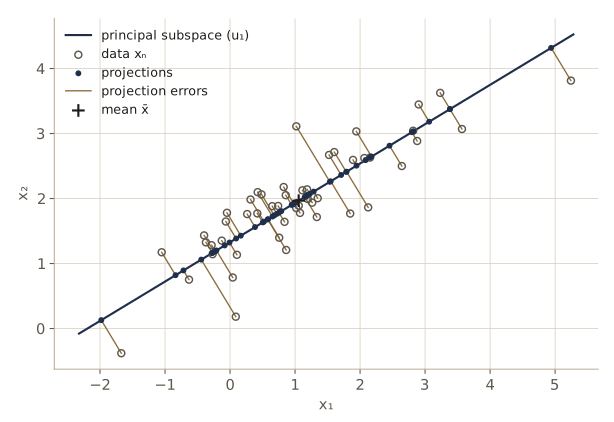
Now the bar images. The covariance is \(256 \times 256\).
xbar, lam, U, S = pca(X_img)
print("five largest eigenvalues:", lam[:5])
print(f"total variance (trace of S): {lam.sum():.4f}")
print(f"fraction captured by M = 3: {lam[:3].sum() / lam.sum():.3f}, "
      f"by M = 10: {lam[:10].sum() / lam.sum():.3f}")
five largest eigenvalues: [1.2594 1.1122 0.4952 0.3926 0.3661]
total variance (trace of S): 5.2768
fraction captured by M = 3: 0.543, by M = 10: 0.844
Three components capture only about half of the variance, even though three numbers generate the data. This is the curvature at work, and we will come back to it with the full eigenvalue spectrum.
Computing all eigenvectors of a \(D \times D\) matrix costs \(O(D^3)\) time. If we need only the leading \(M\), iterative methods such as the power method (multiply a vector by \(\mathbf{S}\) repeatedly and renormalize) cost about \(O(MD^2)\), and the EM algorithm for probabilistic PCA, later in this module, avoids forming \(\mathbf{S}\) at all.
Minimum-error formulation
Now the second definition. Pick any complete orthonormal basis \(\mathbf{u}_1, \dots, \mathbf{u}_D\) of \(\mathbb{R}^D\), so \(\mathbf{u}_i^{\mathrm{T}}\mathbf{u}_j = \delta_{ij}\). Every point can be written exactly in this basis: \(\mathbf{x}_n = \sum_{i=1}^{D} (\mathbf{x}_n^{\mathrm{T}}\mathbf{u}_i)\,\mathbf{u}_i\). That is only a rotation of the axes. To reduce the dimension, we approximate each point using the first \(M\) basis vectors with coefficients \(z_{ni}\) that may depend on the point, and the remaining \(D - M\) basis vectors with coefficients \(b_i\) that are shared by all points:
\[\tilde{\mathbf{x}}_n = \sum_{i=1}^{M} z_{ni}\,\mathbf{u}_i + \sum_{i=M+1}^{D} b_i\,\mathbf{u}_i .\]So each point is described by only \(M\) numbers of its own. We choose the basis, the \(z_{ni}\), and the \(b_i\) to minimize the mean squared error, called the distortion:
\[J = \frac{1}{N}\sum_{n=1}^{N} \lVert \mathbf{x}_n - \tilde{\mathbf{x}}_n \rVert^2 .\]Because the basis is orthonormal, the squared length of a vector is the sum of its squared coordinates, so the error splits coordinate by coordinate:
\[J = \frac{1}{N}\sum_{n=1}^{N} \left[ \sum_{i=1}^{M} \left(\mathbf{x}_n^{\mathrm{T}}\mathbf{u}_i - z_{ni}\right)^2 + \sum_{i=M+1}^{D} \left(\mathbf{x}_n^{\mathrm{T}}\mathbf{u}_i - b_i\right)^2 \right].\]Each \(z_{ni}\) appears in one square only, so the best choice makes that square zero: \(z_{ni} = \mathbf{x}_n^{\mathrm{T}}\mathbf{u}_i\). Each \(b_i\) is shared by \(N\) squares, and the constant that minimizes a sum of squared deviations is the mean: \(b_i = \bar{\mathbf{x}}^{\mathrm{T}}\mathbf{u}_i\). Substituting both,
\[J = \sum_{i=M+1}^{D} \frac{1}{N}\sum_{n=1}^{N} \left(\mathbf{x}_n^{\mathrm{T}}\mathbf{u}_i - \bar{\mathbf{x}}^{\mathrm{T}}\mathbf{u}_i\right)^2 = \sum_{i=M+1}^{D} \mathbf{u}_i^{\mathrm{T}}\mathbf{S}\mathbf{u}_i .\]Two things are already clear. The error vector \(\mathbf{x}_n - \tilde{\mathbf{x}}_n = \sum_{i>M} \left((\mathbf{x}_n - \bar{\mathbf{x}})^{\mathrm{T}}\mathbf{u}_i\right)\mathbf{u}_i\) lies in the span of the discarded directions, so the best approximation is the orthogonal projection onto the subspace through \(\bar{\mathbf{x}}\) spanned by \(\mathbf{u}_1, \dots, \mathbf{u}_M\). And the distortion is the variance along the discarded directions.
It remains to choose the discarded directions. Collect them as the columns of \(\mathbf{U}_\perp\), a \(D \times (D - M)\) matrix with \(\mathbf{U}_\perp^{\mathrm{T}}\mathbf{U}_\perp = \mathbf{I}\), so \(J = \operatorname{Tr}(\mathbf{U}_\perp^{\mathrm{T}}\mathbf{S}\mathbf{U}_\perp)\). Enforce the orthonormality constraints with a symmetric matrix \(\mathbf{H}\) of Lagrange multipliers and make stationary
\[\operatorname{Tr}\left(\mathbf{U}_\perp^{\mathrm{T}}\mathbf{S}\mathbf{U}_\perp\right) - \operatorname{Tr}\left(\mathbf{H}\left(\mathbf{U}_\perp^{\mathrm{T}}\mathbf{U}_\perp - \mathbf{I}\right)\right).\]The gradient with respect to \(\mathbf{U}_\perp\) is \(2\mathbf{S}\mathbf{U}_\perp - 2\mathbf{U}_\perp\mathbf{H}\), so at a stationary point \(\mathbf{S}\mathbf{U}_\perp = \mathbf{U}_\perp\mathbf{H}\). Diagonalize the symmetric matrix \(\mathbf{H} = \mathbf{Q}\boldsymbol{\Lambda}\mathbf{Q}^{\mathrm{T}}\) with \(\mathbf{Q}\) orthogonal. Then \(\mathbf{S}(\mathbf{U}_\perp\mathbf{Q}) = (\mathbf{U}_\perp\mathbf{Q})\boldsymbol{\Lambda}\): the columns of \(\mathbf{U}_\perp\mathbf{Q}\) are eigenvectors of \(\mathbf{S}\), and they span the same space as the columns of \(\mathbf{U}_\perp\). The trace does not change under this rotation, so \(J = \operatorname{Tr}(\boldsymbol{\Lambda})\), the sum of \(D - M\) eigenvalues of \(\mathbf{S}\). The smallest possible value discards the \(D - M\) smallest eigenvalues:
Result. The minimum distortion is achieved by the same principal subspace, spanned by the eigenvectors with the \(M\) largest eigenvalues, and its value is the sum of the discarded eigenvalues, \(J = \sum_{i=M+1}^{D} \lambda_i .\)
The two definitions agree because the total variance \(\operatorname{Tr}(\mathbf{S}) = \sum_i \lambda_i\) is fixed: whatever variance the projection keeps, the error loses, and vice versa. Let us check the formula on the images, and compare with a random subspace of the same dimension.
def distortion(X, B):
    """Mean squared distance from each row of X to its projection onto the
    affine subspace xbar + span(B). B has orthonormal columns."""
    Xc = X - X.mean(axis=0)
    R = Xc - (Xc @ B) @ B.T            # residuals after orthogonal projection
    return np.mean(np.sum(R ** 2, axis=1))

rng_sub = np.random.default_rng(4)
print(" M   J (PCA)   sum of discarded eigenvalues   J (random subspace)")
for M in [1, 3, 10, 30]:
    Q, _ = np.linalg.qr(rng_sub.standard_normal((D, M)))
    print(f"{M:2d}   {distortion(X_img, U[:, :M]):.4f}   {lam[M:].sum():.4f}"
          f"                         {distortion(X_img, Q):.4f}")
 M   J (PCA)   sum of discarded eigenvalues   J (random subspace)
 1   4.0174   4.0174                         5.2661
 3   2.4101   2.4101                         5.2344
10   0.8215   0.8215                         5.0519
30   0.1598   0.1598                         4.6363
The computed distortion matches the sum of the discarded eigenvalues to all printed digits, and a random subspace of the same dimension does far worse.
A related method deserves a sentence. Canonical correlation analysis (CCA) works with two sets of variables measured on the same items and looks for a pair of linear subspaces, one per set, whose projections are highly correlated. Like PCA it reduces to an eigenvalue problem, in its case a generalized one (Bishop §12.1.2).
Applications of PCA
The eigenvalue spectrum. The next figure plots the eigenvalues of the bar data in decreasing order, and the distortion \(J(M)\) that results from keeping \(M\) components.
frac = np.cumsum(lam) / lam.sum()
for target in [0.90, 0.95, 0.99]:
    M_needed = np.searchsorted(frac, target) + 1
    print(f"components needed for {target:.0%} of the variance: {M_needed}")
print(f"noise variance per pixel: {0.02 ** 2:.4f}; "
      f"median eigenvalue: {np.median(lam):.4f}")
components needed for 90% of the variance: 14
components needed for 95% of the variance: 22
components needed for 99% of the variance: 96
noise variance per pixel: 0.0004; median eigenvalue: 0.0005
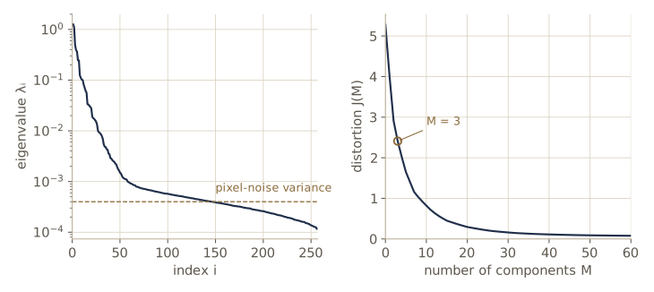
The images have three degrees of freedom, but a flat subspace needs about 20 dimensions to hold 95% of their variance. A curved three-dimensional manifold, seen through linear glasses, looks much higher-dimensional. The spectrum does flatten out eventually, at the level of the pixel noise, and past that point extra components describe only noise.
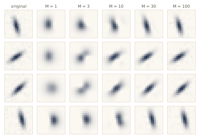
Compression. Substituting the optimal \(z_{ni}\) and \(b_i\) into \(\tilde{\mathbf{x}}_n\) gives the PCA approximation
\[\tilde{\mathbf{x}}_n = \bar{\mathbf{x}} + \sum_{i=1}^{M} \left(\mathbf{x}_n^{\mathrm{T}}\mathbf{u}_i - \bar{\mathbf{x}}^{\mathrm{T}}\mathbf{u}_i\right)\mathbf{u}_i .\]To store the data set we keep \(\bar{\mathbf{x}}\), the \(M\) eigenvectors, and \(M\) numbers per image instead of \(D\). Encoding and decoding are two matrix products:
def pca_encode(X, xbar, U_M):
    """M coordinates per row: z_ni = (x_n - xbar)^T u_i."""
    return (X - xbar) @ U_M

def pca_decode(Z, xbar, U_M):
    """Back to data space: xbar + sum_i z_ni u_i."""
    return xbar + Z @ U_M.T

for M in [1, 3, 10, 30, 100]:
    X_rec = pca_decode(pca_encode(X_img, xbar, U[:, :M]), xbar, U[:, :M])
    rms = np.sqrt(np.mean((X_img - X_rec) ** 2))
    stored = D + M * D + M * N
    print(f"M = {M:3d}: rms pixel error {rms:.4f}, numbers stored {stored:6d}"
          f" ({stored / (N * D):.1%} of the raw data)")
M =   1: rms pixel error 0.1253, numbers stored   1512 (0.6% of the raw data)
M =   3: rms pixel error 0.0970, numbers stored   4024 (1.6% of the raw data)
M =  10: rms pixel error 0.0566, numbers stored  12816 (5.0% of the raw data)
M =  30: rms pixel error 0.0250, numbers stored  37936 (14.8% of the raw data)
M = 100: rms pixel error 0.0140, numbers stored 125856 (49.2% of the raw data)
Standardizing and whitening. PCA is also a preprocessing tool. When variables are measured in different units, a common first step is to standardize: subtract each variable’s mean and divide by its standard deviation, so that every variable has zero mean and unit variance. The covariance of standardized data is the correlation matrix, which still has off-diagonal entries. PCA can go further. Write the eigendecomposition as \(\mathbf{S}\mathbf{U} = \mathbf{U}\mathbf{L}\), with \(\mathbf{L}\) the diagonal matrix of eigenvalues, and define
\[\mathbf{y}_n = \mathbf{L}^{-1/2}\mathbf{U}^{\mathrm{T}}(\mathbf{x}_n - \bar{\mathbf{x}}).\]This rotates the data onto the principal axes and rescales each axis to unit variance. The covariance of the \(\mathbf{y}_n\) is \(\mathbf{L}^{-1/2}\mathbf{U}^{\mathrm{T}}\mathbf{S}\mathbf{U}\mathbf{L}^{-1/2} = \mathbf{L}^{-1/2}\mathbf{L}\mathbf{L}^{-1/2} = \mathbf{I}\): the new variables have zero mean, unit variance, and no correlation. This is called whitening or sphering.
def standardize(X):
    return (X - X.mean(axis=0)) / X.std(axis=0)

def whiten(X):
    """y_n = L^{-1/2} U^T (x_n - xbar). Returns Y and the pieces needed to undo it."""
    xbar, lam, U, _ = pca(X)
    return (X - xbar) @ U / np.sqrt(lam), xbar, lam, U

Xs2 = standardize(X2)
Y2, *_ = whiten(X2)
print("covariance after standardizing:\n", Xs2.T @ Xs2 / len(Xs2))
print("covariance after whitening:\n", Y2.T @ Y2 / len(Y2))
Y_img, *_ = whiten(X_img)
print(f"bar images, 256 x 256 covariance after whitening: max deviation from I = "
      f"{np.abs(Y_img.T @ Y_img / N - np.eye(D)).max():.2e}")
covariance after standardizing:
 [[1.     0.8547]
 [0.8547 1.    ]]
covariance after whitening:
 [[1. 0.]
 [0. 1.]]
bar images, 256 x 256 covariance after whitening: max deviation from I = 6.84e-13
Watch out. Whitening divides by \(\sqrt{\lambda_i}\), so directions with tiny variance, which usually carry nothing but noise, are blown up to the same size as the important ones. For the bar images, well over half of the 256 whitened coordinates carry essentially nothing but pixel noise, now at full volume. In practice we whiten only the leading \(M\) components, or add a small constant to each \(\lambda_i\) before dividing.
Visualization. With \(M = 2\), the coordinates \((z_{n1}, z_{n2})\) place every data point in a plane we can look at. The plane is the one that shows as much of the spread as any linear view can.
Z2 = pca_encode(X_img, xbar, U[:, :2])
cx, cy, theta = latents.T
features = {"cx": cx, "cy": cy,
            "cos 2theta": np.cos(2 * theta), "sin 2theta": np.sin(2 * theta)}
print("correlation of each principal coordinate with the latent variables")
for k in range(2):
    corr = [f"{name} {np.corrcoef(Z2[:, k], f)[0, 1]:+.2f}"
            for name, f in features.items()]
    print(f"  z{k + 1}: " + ", ".join(corr))
correlation of each principal coordinate with the latent variables
  z1: cx +0.92, cy -0.02, cos 2theta +0.00, sin 2theta +0.04
  z2: cx -0.05, cy -0.91, cos 2theta -0.02, sin 2theta +0.07
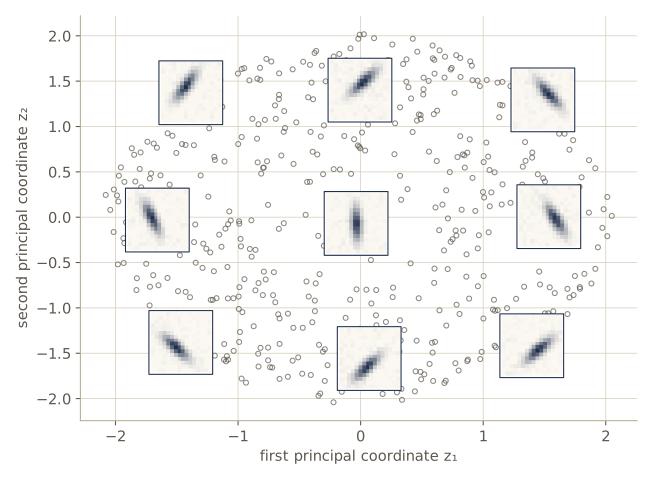
We never told PCA about positions or angles, yet its first two coordinates recover the two position variables almost perfectly (correlations above 0.9 in size; the signs are arbitrary, since \(-\mathbf{u}_i\) is as good an eigenvector as \(\mathbf{u}_i\)). The orientation, which changes the image in a more nonlinear way, is spread over later components.
Watch out. PCA is unsupervised. It keeps the directions of large variance, and those need not be the directions that separate classes. Two elongated classes lying side by side, separated along their short axis, will be projected onto the long axis and mixed completely. For classification, Fisher’s linear discriminant from module 04 uses the labels to choose the projection.
PCA for high-dimensional data
Sometimes there are fewer data points than dimensions: a few hundred images of a million pixels each. Then the \(D \times D\) eigenproblem is expensive, \(O(D^3)\), and wasteful: \(N\) points span an affine subspace of dimension at most \(N - 1\), so at least \(D - N + 1\) eigenvalues are zero.
Let \(\tilde{\mathbf{X}}\) be the \(N \times D\) centered data matrix, whose \(n\)th row is \((\mathbf{x}_n - \bar{\mathbf{x}})^{\mathrm{T}}\), so \(\mathbf{S} = N^{-1}\tilde{\mathbf{X}}^{\mathrm{T}}\tilde{\mathbf{X}}\). The eigenvector equation is \(N^{-1}\tilde{\mathbf{X}}^{\mathrm{T}}\tilde{\mathbf{X}}\mathbf{u}_i = \lambda_i\mathbf{u}_i\). Multiply both sides on the left by \(\tilde{\mathbf{X}}\) and write \(\mathbf{v}_i = \tilde{\mathbf{X}}\mathbf{u}_i\):
\[\frac{1}{N}\tilde{\mathbf{X}}\tilde{\mathbf{X}}^{\mathrm{T}}\mathbf{v}_i = \lambda_i \mathbf{v}_i .\]This is an eigenproblem for an \(N \times N\) matrix, costing \(O(N^3)\), with the same nonzero eigenvalues. To get back to data space, multiply this equation on the left by \(\tilde{\mathbf{X}}^{\mathrm{T}}\): \(N^{-1}\tilde{\mathbf{X}}^{\mathrm{T}}\tilde{\mathbf{X}}(\tilde{\mathbf{X}}^{\mathrm{T}}\mathbf{v}_i) = \lambda_i(\tilde{\mathbf{X}}^{\mathrm{T}}\mathbf{v}_i)\), so \(\tilde{\mathbf{X}}^{\mathrm{T}}\mathbf{v}_i\) is an eigenvector of \(\mathbf{S}\). If \(\mathbf{v}_i\) has unit length, then \(\lVert \tilde{\mathbf{X}}^{\mathrm{T}}\mathbf{v}_i \rVert^2 = \mathbf{v}_i^{\mathrm{T}}\tilde{\mathbf{X}}\tilde{\mathbf{X}}^{\mathrm{T}}\mathbf{v}_i = N\lambda_i\), so the unit eigenvector is
\[\mathbf{u}_i = \frac{1}{\sqrt{N\lambda_i}}\,\tilde{\mathbf{X}}^{\mathrm{T}}\mathbf{v}_i .\]We check it on 100 of the bar images (\(N = 100 < D = 256\)) against the singular value decomposition of \(\tilde{\mathbf{X}}\), whose right singular vectors are the eigenvectors of \(\mathbf{S}\) and whose squared singular values divided by \(N\) are its eigenvalues.
Xs = X_img[:100]
Ns = len(Xs)
Xs_c = Xs - Xs.mean(axis=0)
lam_N, V = np.linalg.eigh(Xs_c @ Xs_c.T / Ns)            # N x N problem
lam_N, V = lam_N[::-1], V[:, ::-1]
k = Ns - 1                      # centering leaves at most N - 1 nonzero eigenvalues
U_trick = Xs_c.T @ V[:, :k] / np.sqrt(Ns * lam_N[:k])

_, sv, Vt = np.linalg.svd(Xs_c, full_matrices=False)     # reference: SVD of the data
S_s = Xs_c.T @ Xs_c / Ns
norms = np.linalg.norm(U_trick, axis=0)
dots = np.abs(np.sum(U_trick[:, :20] * Vt[:20].T, axis=0))
print(f"smallest eigenvalue of the N x N matrix: {lam_N[-1]:.1e}")
ev_diff = np.abs(lam_N[:k] - sv[:k] ** 2 / Ns).max()
print(f"max eigenvalue difference vs SVD: {ev_diff:.1e}")
print(f"column norms of U_trick: {norms.min():.6f} to {norms.max():.6f}")
resid = np.abs(S_s @ U_trick - U_trick * lam_N[:k]).max()
print(f"max residual of S u = lambda u: {resid:.1e}")
print(f"first 20 components, smallest abs(u_trick . u_svd): {dots.min():.6f}")
smallest eigenvalue of the N x N matrix: 3.3e-17
max eigenvalue difference vs SVD: 1.2e-15
column norms of U_trick: 1.000000 to 1.000000
max residual of S u = lambda u: 2.8e-15
first 20 components, smallest abs(u_trick . u_svd): 1.000000
Both routes give the same eigenvalues and the same unit eigenvectors (up to sign). In practice the SVD of \(\tilde{\mathbf{X}}\) is the most stable way to compute PCA in either regime; the Gram-matrix form matters because it is the one that generalizes to kernels, which is how we will use it for kernel PCA.
Probabilistic PCA
PCA as derived so far is a geometric recipe. It has no likelihood, so it cannot be compared with other density models, cannot handle missing values in a principled way, and gives no guidance on \(M\). We now show that PCA is the maximum likelihood solution of a simple latent variable model, probabilistic PCA (PPCA), due to Tipping and Bishop, and harvest the benefits.
The generative model
Introduce an \(M\)-dimensional latent variable \(\mathbf{z}\) with a standard Gaussian prior, and let the observation be a linear function of it plus isotropic Gaussian noise:
\[p(\mathbf{z}) = \mathcal{N}(\mathbf{z} \mid \mathbf{0}, \mathbf{I}), \qquad p(\mathbf{x} \mid \mathbf{z}) = \mathcal{N}(\mathbf{x} \mid \mathbf{W}\mathbf{z} + \boldsymbol{\mu}, \sigma^2\mathbf{I}).\]Here \(\mathbf{W}\) is a \(D \times M\) matrix, \(\boldsymbol{\mu}\) a \(D\)-vector, and \(\sigma^2\) a scalar. Equivalently, \(\mathbf{x} = \mathbf{W}\mathbf{z} + \boldsymbol{\mu} + \boldsymbol{\epsilon}\) with \(\boldsymbol{\epsilon} \sim \mathcal{N}(\mathbf{0}, \sigma^2\mathbf{I})\) independent of \(\mathbf{z}\). To sample, draw \(\mathbf{z}\), map it to the \(M\)-dimensional flat sheet \(\{\mathbf{W}\mathbf{z} + \boldsymbol{\mu}\}\) in data space, and add a small spherical blur. This is a linear-Gaussian model of the kind studied in module 08, and like the naive Bayes model the components of \(\mathbf{x}\) are independent given \(\mathbf{z}\): all correlation between observed variables flows through the latent variables.
We make a synthetic data set from this model with \(D = 10\) and \(M = 3\), and keep a second sample from the same model as a test set.
def ppca_sample(W, mu, sigma2, N, rng):
    """x = W z + mu + eps, z ~ N(0, I), eps ~ N(0, sigma2 I). Returns X and Z."""
    D, M = W.shape
    Z = rng.standard_normal((N, M))
    E = np.sqrt(sigma2) * rng.standard_normal((N, D))
    return Z @ W.T + mu + E, Z

rng_p = np.random.default_rng(3)
D_p, M_p = 10, 3
W_true = rng_p.standard_normal((D_p, M_p)) * np.array([1.5, 1.0, 0.7])
mu_true = rng_p.standard_normal(D_p)
sigma2_true = 0.64
X_p, _ = ppca_sample(W_true, mu_true, sigma2_true, 500, rng_p)
X_test, _ = ppca_sample(W_true, mu_true, sigma2_true, 500, rng_p)
print("training set", X_p.shape, " test set", X_test.shape)
print("eigenvalues of the training covariance:\n", pca(X_p)[1])
training set (500, 10)  test set (500, 10)
eigenvalues of the training covariance:
 [50.1696  7.98    3.9557  0.7882  0.7416  0.7005  0.6538  0.5903  0.5547
  0.5007]
Three large eigenvalues and seven small ones of similar size: three directions of signal, and noise of variance about 0.64 everywhere.
Marginal and posterior distributions
The marginal distribution of \(\mathbf{x}\) is Gaussian because \(\mathbf{x}\) is a linear function of the Gaussian variables \(\mathbf{z}\) and \(\boldsymbol{\epsilon}\). Its mean and covariance follow from \(\mathbf{x} = \mathbf{W}\mathbf{z} + \boldsymbol{\mu} + \boldsymbol{\epsilon}\):
\[\begin{aligned} \mathbb{E}[\mathbf{x}] &= \mathbf{W}\,\mathbb{E}[\mathbf{z}] + \boldsymbol{\mu} + \mathbb{E}[\boldsymbol{\epsilon}] = \boldsymbol{\mu}, \\ \operatorname{cov}[\mathbf{x}] &= \mathbb{E}\left[(\mathbf{W}\mathbf{z} + \boldsymbol{\epsilon})(\mathbf{W}\mathbf{z} + \boldsymbol{\epsilon})^{\mathrm{T}}\right] = \mathbf{W}\mathbf{W}^{\mathrm{T}} + \sigma^2\mathbf{I}, \end{aligned}\]where the cross terms vanish because \(\mathbf{z}\) and \(\boldsymbol{\epsilon}\) are independent with zero mean. So the PPCA marginal is
\[p(\mathbf{x}) = \mathcal{N}(\mathbf{x} \mid \boldsymbol{\mu}, \mathbf{C}), \qquad \mathbf{C} = \mathbf{W}\mathbf{W}^{\mathrm{T}} + \sigma^2\mathbf{I}.\](The same result comes from the general marginal formula for linear-Gaussian models in module 02.) The covariance has a clear shape. Along any direction \(\mathbf{v}\) of unit length, the variance is \(\mathbf{v}^{\mathrm{T}}\mathbf{C}\mathbf{v} = \lVert \mathbf{W}^{\mathrm{T}}\mathbf{v} \rVert^2 + \sigma^2\): exactly \(\sigma^2\) for directions orthogonal to the columns of \(\mathbf{W}\), and more along the sheet. The density is a flattened ellipsoid, a pancake in three dimensions.
Two structural facts follow. First, a rotational ambiguity: if \(\mathbf{R}\) is any \(M \times M\) orthogonal matrix, then \(\mathbf{W}\mathbf{R}\) gives the same \(\mathbf{C}\), because
\[(\mathbf{W}\mathbf{R})(\mathbf{W}\mathbf{R})^{\mathrm{T}} = \mathbf{W}\mathbf{R}\mathbf{R}^{\mathrm{T}}\mathbf{W}^{\mathrm{T}} = \mathbf{W}\mathbf{W}^{\mathrm{T}}.\]The data cannot tell \(\mathbf{W}\) from \(\mathbf{W}\mathbf{R}\); rotating the latent space, whose prior is spherical, changes nothing observable. Second, a parameter count: \(\mathbf{C}\) is determined by \(DM + 1\) numbers minus the \(M(M-1)/2\) degrees of freedom of an orthogonal \(\mathbf{R}\). That is linear in \(D\), where a full covariance needs \(D(D+1)/2\).
def ppca_n_params(D, M):
    """Parameters of C = W W^T + sigma^2 I (Bishop eq. 12.51), plus D for the mean."""
    return D * M + 1 - M * (M - 1) // 2 + D

for D_, M_ in [(10, 3), (256, 10)]:
    print(f"D = {D_:3d}, M = {M_:2d}: PPCA {ppca_n_params(D_, M_):5d} parameters,"
          f" full-covariance Gaussian {D_ * (D_ + 1) // 2 + D_:5d}")

rng_big = np.random.default_rng(5)
X_many, _ = ppca_sample(W_true, mu_true, sigma2_true, 200_000, rng_big)
C_true = W_true @ W_true.T + sigma2_true * np.eye(D_p)
err = np.abs(np.cov(X_many.T, bias=True) - C_true).max()
print(f"200,000 samples: max abs(sample cov - C) = {err:.4f}"
      f" (entries of C up to {np.abs(C_true).max():.2f})")
R = np.linalg.qr(rng_big.standard_normal((M_p, M_p)))[0]   # random orthogonal matrix
WR = W_true @ R
change = np.abs(WR @ WR.T - W_true @ W_true.T).max()
print(f"rotating W: max change in C = {change:.1e}")
D =  10, M =  3: PPCA    38 parameters, full-covariance Gaussian    65
D = 256, M = 10: PPCA  2772 parameters, full-covariance Gaussian 33152
200,000 samples: max abs(sample cov - C) = 0.0630 (entries of C up to 25.60)
rotating W: max change in C = 7.1e-15
Evaluating \(p(\mathbf{x})\) needs \(\mathbf{C}^{-1}\), a \(D \times D\) inverse. The matrix inversion identity from Appendix C (the Woodbury identity) turns it into an \(M \times M\) problem. Define
\[\mathbf{M} = \mathbf{W}^{\mathrm{T}}\mathbf{W} + \sigma^2\mathbf{I} \qquad (M \times M).\]Then
\[\mathbf{C}^{-1} = \sigma^{-2}\left(\mathbf{I} - \mathbf{W}\mathbf{M}^{-1}\mathbf{W}^{\mathrm{T}}\right), \qquad \lvert \mathbf{C} \rvert = \sigma^{2(D-M)}\lvert \mathbf{M} \rvert .\]You can confirm the first by multiplying it with \(\mathbf{C}\) and using \(\mathbf{W}^{\mathrm{T}}\mathbf{W} = \mathbf{M} - \sigma^2\mathbf{I}\); the second follows from the determinant identity (Appendix C)
\[\lvert \sigma^2\mathbf{I}_D + \mathbf{W}\mathbf{W}^{\mathrm{T}} \rvert = \sigma^{2D}\lvert \mathbf{I}_M + \sigma^{-2}\mathbf{W}^{\mathrm{T}}\mathbf{W} \rvert .\]The posterior \(p(\mathbf{z} \mid \mathbf{x})\) comes from the linear-Gaussian formulas of module 02 (Bishop eq. 2.116). The posterior precision is the prior precision plus the precision contributed by the observation, \(\mathbf{I} + \sigma^{-2}\mathbf{W}^{\mathrm{T}}\mathbf{W} = \sigma^{-2}\mathbf{M}\), and the posterior mean is that covariance times \(\sigma^{-2}\mathbf{W}^{\mathrm{T}}(\mathbf{x} - \boldsymbol{\mu})\):
\[p(\mathbf{z} \mid \mathbf{x}) = \mathcal{N}\left(\mathbf{z} \mid \mathbf{M}^{-1}\mathbf{W}^{\mathrm{T}}(\mathbf{x} - \boldsymbol{\mu}),\ \sigma^2\mathbf{M}^{-1}\right).\]The posterior covariance does not depend on \(\mathbf{x}\).
We check both formulas against brute force: \(\mathbf{C}^{-1}\) against a direct inverse (we use np.linalg.inv only for this check; elsewhere we solve linear systems), and the posterior against conditioning the joint Gaussian of \((\mathbf{z}, \mathbf{x})\), whose covariance is \(\begin{pmatrix} \mathbf{I} & \mathbf{W}^{\mathrm{T}} \\ \mathbf{W} & \mathbf{C} \end{pmatrix}\).
def ppca_posterior(X, W, mu, sigma2):
    """Posterior means (one row per data point) and shared covariance of p(z | x)."""
    M = W.shape[1]
    Mmat = W.T @ W + sigma2 * np.eye(M)
    means = np.linalg.solve(Mmat, W.T @ (X - mu).T).T      # M^{-1} W^T (x - mu)
    cov = sigma2 * np.linalg.inv(Mmat)                      # small M x M inverse
    return means, cov

W, mu, sigma2 = W_true, mu_true, sigma2_true
Mmat = W.T @ W + sigma2 * np.eye(M_p)
C_inv_woodbury = (np.eye(D_p) - W @ np.linalg.solve(Mmat, W.T)) / sigma2
diff = np.abs(C_inv_woodbury - np.linalg.inv(C_true)).max()
print(f"Woodbury C^-1 vs direct inverse: max diff {diff:.1e}")
print(f"log det C: direct {np.linalg.slogdet(C_true)[1]:.6f}, "
      f"via M {(D_p - M_p) * np.log(sigma2) + np.linalg.slogdet(Mmat)[1]:.6f}")

x = X_p[:1]
m_post, S_post = ppca_posterior(x, W, mu, sigma2)
m_joint = W.T @ np.linalg.solve(C_true, (x - mu).ravel())   # condition the joint
S_joint = np.eye(M_p) - W.T @ np.linalg.solve(C_true, W)
print("posterior mean:", m_post.ravel(), " joint-Gaussian:", m_joint)
print(f"posterior covariance max diff: {np.abs(S_post - S_joint).max():.1e}")
Woodbury C^-1 vs direct inverse: max diff 2.7e-15
log det C: direct 4.410339, via M 4.410339
posterior mean: [ 0.2292  0.411  -0.3005]  joint-Gaussian: [ 0.2292  0.411  -0.3005]
posterior covariance max diff: 1.6e-16
Maximum likelihood PCA
Given data \(\mathbf{X}\), the log-likelihood of the parameters is a sum of Gaussian log densities,
\[\ln p(\mathbf{X} \mid \boldsymbol{\mu}, \mathbf{W}, \sigma^2) = -\frac{ND}{2}\ln(2\pi) - \frac{N}{2}\ln\lvert \mathbf{C} \rvert - \frac{1}{2}\sum_{n=1}^{N} (\mathbf{x}_n - \boldsymbol{\mu})^{\mathrm{T}}\mathbf{C}^{-1}(\mathbf{x}_n - \boldsymbol{\mu}).\]Setting the derivative with respect to \(\boldsymbol{\mu}\) to zero gives \(\boldsymbol{\mu}_{\mathrm{ML}} = \bar{\mathbf{x}}\), as for any Gaussian. With that substituted, the quadratic term becomes a trace against the sample covariance, and
\[\ln p(\mathbf{X} \mid \bar{\mathbf{x}}, \mathbf{W}, \sigma^2) = -\frac{N}{2}\left\{ D\ln(2\pi) + \ln\lvert \mathbf{C} \rvert + \operatorname{Tr}\left(\mathbf{C}^{-1}\mathbf{S}\right) \right\}.\]The data enter only through \(\mathbf{S}\). Maximizing over \(\mathbf{W}\) and \(\sigma^2\) looks hard, since \(\mathbf{C}\) depends on them nonlinearly, but it has an exact solution. We sketch the derivation (Tipping and Bishop give every detail).
Stationary points in \(\mathbf{W}\). Using \(\partial \ln\lvert\mathbf{C}\rvert = \operatorname{Tr}(\mathbf{C}^{-1}\partial\mathbf{C})\) and \(\partial\,\mathbf{C}^{-1} = -\mathbf{C}^{-1}(\partial\mathbf{C})\mathbf{C}^{-1}\) from Appendix C, with \(\partial\mathbf{C} = (\partial\mathbf{W})\mathbf{W}^{\mathrm{T}} + \mathbf{W}(\partial\mathbf{W})^{\mathrm{T}}\), the gradient is
\[\frac{\partial}{\partial\mathbf{W}} \ln p = N\left(\mathbf{C}^{-1}\mathbf{S}\mathbf{C}^{-1}\mathbf{W} - \mathbf{C}^{-1}\mathbf{W}\right).\]Setting it to zero and multiplying by \(\mathbf{C}\) on the left gives \(\mathbf{S}\mathbf{C}^{-1}\mathbf{W} = \mathbf{W}\). Now a small identity: \(\mathbf{C}\mathbf{W} = \mathbf{W}\mathbf{W}^{\mathrm{T}}\mathbf{W} + \sigma^2\mathbf{W} = \mathbf{W}\mathbf{M}\), so \(\mathbf{C}^{-1}\mathbf{W} = \mathbf{W}\mathbf{M}^{-1}\). The condition becomes \(\mathbf{S}\mathbf{W}\mathbf{M}^{-1} = \mathbf{W}\), that is,
\[\mathbf{S}\mathbf{W} = \mathbf{W}\left(\mathbf{W}^{\mathrm{T}}\mathbf{W} + \sigma^2\mathbf{I}\right).\]Write \(\mathbf{W}\) through its singular value decomposition, \(\mathbf{W} = \mathbf{V}\mathbf{\Lambda}_W\mathbf{R}\), with \(\mathbf{V}\) a \(D \times M\) matrix of orthonormal columns \(\mathbf{v}_i\), \(\mathbf{\Lambda}_W = \operatorname{diag}(l_1, \dots, l_M)\), and \(\mathbf{R}\) orthogonal. Then \(\mathbf{W}^{\mathrm{T}}\mathbf{W} = \mathbf{R}^{\mathrm{T}}\mathbf{\Lambda}_W^2\mathbf{R}\), and after cancelling \(\mathbf{R}\) on the right the condition reads \(\mathbf{S}\mathbf{V}\mathbf{\Lambda}_W = \mathbf{V}\mathbf{\Lambda}_W(\mathbf{\Lambda}_W^2 + \sigma^2\mathbf{I})\). Column by column, for each \(l_i \ne 0\):
\[\mathbf{S}\mathbf{v}_i = (l_i^2 + \sigma^2)\,\mathbf{v}_i .\]So each \(\mathbf{v}_i\) is an eigenvector of \(\mathbf{S}\), with eigenvalue \(\lambda_i = l_i^2 + \sigma^2\), which fixes \(l_i = \sqrt{\lambda_i - \sigma^2}\). (Columns with \(l_i = 0\) are also stationary; they correspond to leaving a latent dimension unused.)
The noise variance. At such a point, \(\mathbf{C}\) has eigenvector \(\mathbf{v}_i\) with eigenvalue \(l_i^2 + \sigma^2 = \lambda_i\) for each retained direction, and eigenvalue \(\sigma^2\) on the other \(D - M\) eigenvectors of \(\mathbf{S}\). Hence \(\ln\lvert\mathbf{C}\rvert = \sum_{\text{kept}}\ln\lambda_i + (D - M)\ln\sigma^2\) and \(\operatorname{Tr}(\mathbf{C}^{-1}\mathbf{S}) = M + \sigma^{-2}\sum_{\text{discarded}}\lambda_i\). Minimizing \((D - M)\ln\sigma^2 + \sigma^{-2}\sum_{\text{discarded}}\lambda_i\) over \(\sigma^2\) gives the average of the discarded eigenvalues.
Which eigenvectors. Substituting back, the log-likelihood at a stationary point is
\[-\frac{N}{2}\left\{ D\ln(2\pi) + \sum_{\text{kept}}\ln\lambda_i + (D - M)\ln\left(\frac{1}{D - M}\sum_{\text{discarded}}\lambda_i\right) + D \right\}.\]Because the logarithm is concave, the log of an average is at least the average of the logs, and the expression is largest when the discarded eigenvalues are as small as possible, that is, when we keep the \(M\) largest. The other stationary points are saddle points (Tipping and Bishop, 1999).
Result. The maximum likelihood PPCA parameters are \(\boldsymbol{\mu}_{\mathrm{ML}} = \bar{\mathbf{x}}\), the noise variance \(\sigma^2_{\mathrm{ML}} = \frac{1}{D - M}\sum_{i=M+1}^{D}\lambda_i\) (the average of the discarded eigenvalues), and \(\mathbf{W}_{\mathrm{ML}} = \mathbf{U}_M\left(\mathbf{L}_M - \sigma^2_{\mathrm{ML}}\mathbf{I}\right)^{1/2}\mathbf{R}\), where \(\mathbf{U}_M\) holds the eigenvectors of \(\mathbf{S}\) with the \(M\) largest eigenvalues, \(\mathbf{L}_M\) is the diagonal matrix of those eigenvalues, and \(\mathbf{R}\) is any \(M \times M\) orthogonal matrix.
The model keeps the observed variance \(\lambda_i\) along each principal direction exactly, and replaces the variance in all the discarded directions by their average. Let us implement it, and check it three ways: the log-likelihood computed with a Cholesky factor against scipy.stats and against the closed-form expression above; the gradient at the solution, which should vanish; and the effect of moving away from the solution.
def ppca_ml(X, M):
    """Closed-form maximum likelihood PPCA (with R = I)."""
    xbar, lam, U, _ = pca(X)
    sigma2 = lam[M:].mean()
    W = U[:, :M] * np.sqrt(lam[:M] - sigma2)
    return xbar, W, sigma2

def gauss_loglik(X, mu, C):
    """sum_n ln N(x_n | mu, C) using a Cholesky factor C = L L^T."""
    N, D = X.shape
    L = np.linalg.cholesky(C)
    Y = solve_triangular(L, (X - mu).T, lower=True)
    log_det = 2 * np.sum(np.log(np.diag(L)))
    return -0.5 * (N * D * np.log(2 * np.pi) + N * log_det + np.sum(Y ** 2))

def ppca_loglik(X, mu, W, sigma2):
    return gauss_loglik(X, mu, W @ W.T + sigma2 * np.eye(X.shape[1]))

mu_ml, W_ml, s2_ml = ppca_ml(X_p, 3)
lam_p = pca(X_p)[1]
Np = len(X_p)
print(f"sigma2_ML = {s2_ml:.4f} (true 0.64); "
      f"mean of the 7 discarded eigenvalues = {lam_p[3:].mean():.4f}")

ll = ppca_loglik(X_p, mu_ml, W_ml, s2_ml)
C_ml = W_ml @ W_ml.T + s2_ml * np.eye(D_p)
ll_scipy = stats.multivariate_normal(mu_ml, C_ml).logpdf(X_p).sum()
ll_formula = -Np / 2 * (D_p * np.log(2 * np.pi) + np.log(lam_p[:3]).sum()
                        + (D_p - 3) * np.log(s2_ml) + D_p)
print(f"log-likelihood: Cholesky {ll:.4f}, scipy {ll_scipy:.4f}, "
      f"closed form {ll_formula:.4f}")

def num_grad(f, theta, h=1e-5):
    g = np.zeros_like(theta)
    for i in range(theta.size):
        e = np.zeros_like(theta); e[i] = h
        g[i] = (f(theta + e) - f(theta - e)) / (2 * h)
    return g

theta_ml = np.append(W_ml.ravel(), s2_ml)
f = lambda th: ppca_loglik(X_p, mu_ml, th[:-1].reshape(D_p, 3), th[-1])
grad = num_grad(f, theta_ml)
print(f"max abs numerical gradient at the ML solution: {np.abs(grad).max():.1e}")
sigma2_ML = 0.6471 (true 0.64); mean of the 7 discarded eigenvalues = 0.6471
log-likelihood: Cholesky -8174.9259, scipy -8174.9259, closed form -8174.9259
max abs numerical gradient at the ML solution: 4.1e-07
All three log-likelihood evaluations agree, and the gradient with respect to all 31 parameters is zero up to finite-difference error. Now the other claims: rotations of \(\mathbf{W}\) leave the likelihood unchanged, small perturbations lower it, and the stationary point that leaves one latent dimension unused (a zero column) is far worse.
rng_chk = np.random.default_rng(6)
R = np.linalg.qr(rng_chk.standard_normal((3, 3)))[0]
ll_rot = ppca_loglik(X_p, mu_ml, W_ml @ R, s2_ml)
print(f"W R, random rotation: change {ll_rot - ll:+.1e}")
for scale in [0.01, 0.1]:
    changes = []
    for _ in range(5):
        W_pert = W_ml + scale * rng_chk.standard_normal(W_ml.shape)
        changes.append(ppca_loglik(X_p, mu_ml, W_pert, s2_ml) - ll)
    print(f"random perturbations of size {scale}: "
          f"change between {min(changes):+.3f} and {max(changes):+.3f}")
_, lam_p, U_p, _ = pca(X_p)
s2_two = lam_p[2:].mean()                # stationary point that uses only 2 columns
W_two = np.column_stack([U_p[:, :2] * np.sqrt(lam_p[:2] - s2_two), np.zeros(D_p)])
print(f"third column zero: change {ppca_loglik(X_p, mu_ml, W_two, s2_two) - ll:+.3f}")
W R, random rotation: change +0.0e+00
random perturbations of size 0.01: change between -1.280 and -0.585
random perturbations of size 0.1: change between -83.236 and -50.021
third column zero: change -535.705
Choosing \(M\) with held-out data. Because PPCA has a likelihood, we can compare models of different latent dimension on data they were not fitted to. The training log-likelihood always increases with \(M\); the test log-likelihood should peak near the true value.
print(" M   train ln p / N   test ln p / N   parameters")
for M in range(1, 8):
    mu_M, W_M, s2_M = ppca_ml(X_p, M)
    print(f"{M:2d}   {ppca_loglik(X_p, mu_M, W_M, s2_M) / 500:12.4f}"
          f"   {ppca_loglik(X_test, mu_M, W_M, s2_M) / 500:12.4f}"
          f"   {ppca_n_params(D_p, M):8d}")
 M   train ln p / N   test ln p / N   parameters
 1       -18.8653       -19.0612         21
 2       -17.4213       -17.3685         30
 3       -16.3499       -16.3226         38
 4       -16.3374       -16.3344         45
 5       -16.3276       -16.3361         51
 6       -16.3195       -16.3389         56
 7       -16.3136       -16.3386         60
The test log-likelihood rises steeply up to \(M = 3\), peaks there, and then drifts slightly down, while the training value keeps creeping up: the extra dimensions fit noise in the training set. Cross-validation of this kind works, but it gets expensive when there are many models to compare, for instance one \(M\) per component in a mixture. Bayesian PCA, below, is an alternative.
Projecting data. PPCA maps a data point to a distribution over \(\mathbf{z}\) rather than to a point, and the natural summary is the posterior mean \(\mathbb{E}[\mathbf{z} \mid \mathbf{x}] = \mathbf{M}^{-1}\mathbf{W}^{\mathrm{T}}(\mathbf{x} - \bar{\mathbf{x}})\). Mapped back to data space it gives \(\mathbf{W}\,\mathbb{E}[\mathbf{z} \mid \mathbf{x}] + \bar{\mathbf{x}}\). At the ML solution, with \(\mathbf{R} = \mathbf{I}\),
\[\mathbf{W}\mathbf{M}^{-1}\mathbf{W}^{\mathrm{T}} = \mathbf{U}_M\operatorname{diag}\left(\frac{\lambda_i - \sigma^2}{\lambda_i}\right)\mathbf{U}_M^{\mathrm{T}} ,\]which is the orthogonal projection of PCA, but with each principal coordinate shrunk toward the mean by the factor \((\lambda_i - \sigma^2)/\lambda_i < 1\). As \(\sigma^2 \to 0\), \(\mathbf{M}^{-1}\mathbf{W}^{\mathrm{T}} \to (\mathbf{W}^{\mathrm{T}}\mathbf{W})^{-1}\mathbf{W}^{\mathrm{T}}\) and the shrinkage disappears; we recover standard PCA.
Ez, _ = ppca_posterior(X_p, W_ml, mu_ml, s2_ml)
recon_ppca = Ez @ W_ml.T                                  # W E[z | x], minus the mean
recon_pca = pca_encode(X_p, mu_ml, U_p[:, :3]) @ U_p[:, :3].T   # orthogonal projection
coef = (recon_ppca @ U_p[:, :3]) / (recon_pca @ U_p[:, :3])
print("shrinkage along each principal direction:", coef.mean(axis=0))
print(f"  (spread over data points {coef.std(axis=0).max():.1e})")
print("(lambda_i - sigma2) / lambda_i:          ", (lam_p[:3] - s2_ml) / lam_p[:3])
shrinkage along each principal direction: [0.9871 0.9189 0.8364]
  (spread over data points 1.1e-14)
(lambda_i - sigma2) / lambda_i:           [0.9871 0.9189 0.8364]
The posterior mean is a shrunken projection because it balances two sources of information: the prior says \(\mathbf{z}\) is probably near 0, and the observation says it is near the orthogonal projection. The weaker the signal in a direction relative to the noise, the more the prior wins. This is the same trade-off as between the prior mean and the data in Bayesian linear regression (module 03).
EM algorithm for PCA
The closed form needs the eigendecomposition of \(\mathbf{S}\). The EM algorithm of module 09 gives an iterative alternative that is cheaper in high dimensions, extends to missing data, and carries over to factor analysis, where there is no closed form.
The latent variables are the \(\mathbf{z}_n\). The complete-data log-likelihood is \(\sum_n \left\{\ln p(\mathbf{x}_n \mid \mathbf{z}_n) + \ln p(\mathbf{z}_n)\right\}\). Writing out the two Gaussians and taking the expectation under the posterior of each \(\mathbf{z}_n\) (we set \(\boldsymbol{\mu} = \bar{\mathbf{x}}\) at once), we get
\[\begin{aligned} \mathbb{E}[\ln p(\mathbf{X}, \mathbf{Z})] = -\sum_{n=1}^{N}\Big\{ & \frac{D}{2}\ln(2\pi\sigma^2) + \frac{1}{2}\operatorname{Tr}\left(\mathbb{E}[\mathbf{z}_n\mathbf{z}_n^{\mathrm{T}}]\right) + \frac{1}{2\sigma^2}\lVert \mathbf{x}_n - \bar{\mathbf{x}} \rVert^2 \\ & - \frac{1}{\sigma^2}\mathbb{E}[\mathbf{z}_n]^{\mathrm{T}}\mathbf{W}^{\mathrm{T}}(\mathbf{x}_n - \bar{\mathbf{x}}) + \frac{1}{2\sigma^2}\operatorname{Tr}\left(\mathbb{E}[\mathbf{z}_n\mathbf{z}_n^{\mathrm{T}}]\,\mathbf{W}^{\mathrm{T}}\mathbf{W}\right) \Big\} \end{aligned}\]plus a constant. Only two posterior moments appear, and both come from the posterior we derived:
E step.
\[\mathbb{E}[\mathbf{z}_n] = \mathbf{M}^{-1}\mathbf{W}^{\mathrm{T}}(\mathbf{x}_n - \bar{\mathbf{x}}), \qquad \mathbb{E}[\mathbf{z}_n\mathbf{z}_n^{\mathrm{T}}] = \sigma^2\mathbf{M}^{-1} + \mathbb{E}[\mathbf{z}_n]\mathbb{E}[\mathbf{z}_n]^{\mathrm{T}}.\]M step. The expected log-likelihood is quadratic in \(\mathbf{W}\). Its gradient is
\[\frac{1}{\sigma^2}\sum_{n=1}^{N}\left\{(\mathbf{x}_n - \bar{\mathbf{x}})\,\mathbb{E}[\mathbf{z}_n]^{\mathrm{T}} - \mathbf{W}\,\mathbb{E}[\mathbf{z}_n\mathbf{z}_n^{\mathrm{T}}]\right\}.\]Setting it to zero, and then setting the derivative with respect to \(\sigma^2\) to zero with the new \(\mathbf{W}\), gives
\[\begin{aligned} \mathbf{W}_{\text{new}} &= \left[\sum_{n=1}^{N}(\mathbf{x}_n - \bar{\mathbf{x}})\,\mathbb{E}[\mathbf{z}_n]^{\mathrm{T}}\right]\left[\sum_{n=1}^{N}\mathbb{E}[\mathbf{z}_n\mathbf{z}_n^{\mathrm{T}}]\right]^{-1}, \\ \sigma^2_{\text{new}} &= \frac{1}{ND}\sum_{n=1}^{N}\Big\{ \lVert \mathbf{x}_n - \bar{\mathbf{x}} \rVert^2 - 2\,\mathbb{E}[\mathbf{z}_n]^{\mathrm{T}}\mathbf{W}_{\text{new}}^{\mathrm{T}}(\mathbf{x}_n - \bar{\mathbf{x}}) \\ &\qquad\qquad + \operatorname{Tr}\left(\mathbb{E}[\mathbf{z}_n\mathbf{z}_n^{\mathrm{T}}]\,\mathbf{W}_{\text{new}}^{\mathrm{T}}\mathbf{W}_{\text{new}}\right) \Big\}. \end{aligned}\]The first line is a least-squares regression of the data on the expected latent variables, with the second moment standing in for \(\mathbf{Z}^{\mathrm{T}}\mathbf{Z}\). We measure agreement between the EM subspace and the closed-form one by principal angles: for two \(M\)-dimensional subspaces with orthonormal bases \(\mathbf{Q}_a\) and \(\mathbf{Q}_b\), the singular values of \(\mathbf{Q}_a^{\mathrm{T}}\mathbf{Q}_b\) are the cosines of \(M\) angles, all zero exactly when the subspaces coincide. (For small angles the cosines are all close to 1, so the code computes the sines instead, as the singular values of \(\mathbf{Q}_b - \mathbf{Q}_a\mathbf{Q}_a^{\mathrm{T}}\mathbf{Q}_b\).) Angles are the right comparison because EM can converge to any \(\mathbf{W}_{\mathrm{ML}}\mathbf{R}\).
def principal_angles(A, B):
    """Principal angles (degrees, smallest first) between the column spaces of A, B."""
    Qa, _ = np.linalg.qr(A)
    Qb, _ = np.linalg.qr(B)
    # singular values of (I - Qa Qa^T) Qb = sines of the angles (accurate when small)
    sines = np.linalg.svd(Qb - Qa @ (Qa.T @ Qb), compute_uv=False)
    return np.sort(np.degrees(np.arcsin(np.clip(sines, 0.0, 1.0))))

def ppca_em(X, M, n_iter, rng, report=()):
    """EM for probabilistic PCA. Returns xbar, W, sigma2."""
    N, D = X.shape
    xbar = X.mean(axis=0)
    Xc = X - xbar
    W = rng.standard_normal((D, M))
    sigma2 = 1.0
    for it in range(1, n_iter + 1):
        # E step: posterior moments of every z_n
        Mmat = W.T @ W + sigma2 * np.eye(M)
        Ez = np.linalg.solve(Mmat, W.T @ Xc.T).T                  # rows are E[z_n]
        sum_Ezz = N * sigma2 * np.linalg.inv(Mmat) + Ez.T @ Ez    # sum_n E[z_n z_n^T]
        # M step
        W = np.linalg.solve(sum_Ezz, Ez.T @ Xc).T   # (sum x E[z]^T)(sum E[zz^T])^-1
        sigma2 = (np.sum(Xc ** 2) - 2 * np.sum(Ez * (Xc @ W))
                  + np.trace(sum_Ezz @ W.T @ W)) / (N * D)
        if it in report:
            ll_it = ppca_loglik(X, xbar, W, sigma2)
            angle = principal_angles(W, W_ml).max()
            print(f"iter {it:3d}: ln p = {ll_it:10.4f}, sigma2 = {sigma2:.5f}, "
                  f"max angle to W_ML {angle:.1e} deg")
    return xbar, W, sigma2

_, W_em, s2_em = ppca_em(X_p, 3, 500, np.random.default_rng(0),
                         report=(1, 2, 5, 20, 100, 500))
print(f"closed form:  ln p = {ll:10.4f}, sigma2 = {s2_ml:.5f}")
iter   1: ln p = -9160.4824, sigma2 = 1.83507, max angle to W_ML 3.5e+01 deg
iter   2: ln p = -8473.0613, sigma2 = 1.06665, max angle to W_ML 6.2e+00 deg
iter   5: ln p = -8232.8177, sigma2 = 0.66398, max angle to W_ML 2.9e-02 deg
iter  20: ln p = -8191.6232, sigma2 = 0.64776, max angle to W_ML 5.4e-13 deg
iter 100: ln p = -8175.1047, sigma2 = 0.64717, max angle to W_ML 8.0e-14 deg
iter 500: ln p = -8174.9259, sigma2 = 0.64712, max angle to W_ML 9.1e-14 deg
closed form:  ln p = -8174.9259, sigma2 = 0.64712
The log-likelihood increases at every checkpoint, as EM guarantees. The subspace locks on within a handful of iterations, while \(\sigma^2\) and the lengths of the columns of \(\mathbf{W}\), which trade off against each other, settle more slowly. In the end EM reaches the closed-form likelihood.
Each EM iteration costs \(O(NDM)\): we never form the \(D \times D\) covariance. When \(D\) is large and \(M\) small this beats the \(O(ND^2)\) cost of building \(\mathbf{S}\) and the \(O(D^3)\) cost of its full eigendecomposition. EM also handles data with values missing at random: the missing entries of each \(\mathbf{x}_n\) are treated as extra latent variables and filled in, in expectation, in the E step (Bishop §12.2.2, Exercise 12.16).
The zero-noise limit. Let \(\sigma^2 \to 0\) in the EM updates. The E step becomes an ordinary least-squares projection, and the M step a least-squares fit of \(\mathbf{W}\). With \(\tilde{\mathbf{X}}\) the centered \(N \times D\) data matrix and \(\mathbf{\Omega}\) the \(M \times N\) matrix whose columns are the \(\mathbb{E}[\mathbf{z}_n]\):
\[\mathbf{\Omega} = (\mathbf{W}_{\text{old}}^{\mathrm{T}}\mathbf{W}_{\text{old}})^{-1}\mathbf{W}_{\text{old}}^{\mathrm{T}}\tilde{\mathbf{X}}^{\mathrm{T}}, \qquad \mathbf{W}_{\text{new}} = \tilde{\mathbf{X}}^{\mathrm{T}}\mathbf{\Omega}^{\mathrm{T}}(\mathbf{\Omega}\mathbf{\Omega}^{\mathrm{T}})^{-1}.\]This is alternating least squares on the reconstruction error \(\sum_n \lVert \mathbf{x}_n - \bar{\mathbf{x}} - \mathbf{W}\mathbf{z}_n \rVert^2\): fix the subspace and find each point’s best coordinates (its orthogonal projection), then fix the coordinates and find the best subspace. A mechanical picture helps: tie each data point to a rigid rod (the subspace) with a spring. In the E step, the attachment points slide along the fixed rod to where the springs are shortest; in the M step, the attachment points are held and the rod moves to the position of least spring energy. We run it on the bar images, with \(M = 5\), without ever forming the \(256 \times 256\) covariance.
def pca_em_zero_noise(X, M, n_iter, rng, report=(), reference=None):
    """EM for PCA as sigma^2 -> 0. The columns of W span the principal subspace."""
    Xc = X - X.mean(axis=0)
    W = rng.standard_normal((X.shape[1], M))
    for it in range(1, n_iter + 1):
        Omega = np.linalg.solve(W.T @ W, W.T @ Xc.T)        # E step: M x N coordinates
        W = np.linalg.solve(Omega @ Omega.T, Omega @ Xc).T       # M step: D x M
        if it in report:
            angle = principal_angles(W, reference).max()
            print(f"iter {it:3d}: max angle to the top-5 eigenvectors {angle:.2e} deg")
    return W

W_zn = pca_em_zero_noise(X_img, 5, 60, np.random.default_rng(1),
                         report=(1, 5, 20, 60), reference=U[:, :5])
print("eigenvalue ratio lambda_6 / lambda_5 =", f"{lam[5] / lam[4]:.3f}")
iter   1: max angle to the top-5 eigenvectors 7.24e+01 deg
iter   5: max angle to the top-5 eigenvectors 1.57e+01 deg
iter  20: max angle to the top-5 eigenvectors 2.52e-02 deg
iter  60: max angle to the top-5 eigenvectors 2.76e-09 deg
eigenvalue ratio lambda_6 / lambda_5 = 0.674
Once close, the angle shrinks by a roughly constant factor per iteration, like the power method: between iterations 20 and 60 it falls by about 1.5 per step, close to \(\lambda_5/\lambda_6 = 1/0.674\). The rate depends on the gap between \(\lambda_M\) and \(\lambda_{M+1}\): the smaller the ratio \(\lambda_{M+1}/\lambda_M\), the faster the convergence.
In practice, for moderate \(D\), compute PCA with an SVD of the centered data. EM for PCA earns its place when \(D\) is very large, when only a few components are needed, when values are missing, or as a building block inside larger probabilistic models such as mixtures of PPCA.
Bayesian PCA
Held-out likelihood let us choose \(M\), but a Bayesian treatment can do it inside a single fit. The idea is automatic relevance determination (ARD), which we met for the relevance vector machine in module 07. Give each column \(\mathbf{w}_i\) of \(\mathbf{W}\) its own zero-mean Gaussian prior with precision \(\alpha_i\):
\[p(\mathbf{W} \mid \boldsymbol{\alpha}) = \prod_{i=1}^{M}\left(\frac{\alpha_i}{2\pi}\right)^{D/2}\exp\left(-\frac{1}{2}\alpha_i\mathbf{w}_i^{\mathrm{T}}\mathbf{w}_i\right).\]The hyperparameters \(\alpha_i\) are chosen to maximize the marginal likelihood, in which \(\mathbf{W}\) is integrated out. If a latent direction does not help explain the data, its \(\alpha_i\) is driven to infinity and its column \(\mathbf{w}_i\) to zero; that dimension is switched off. Start with a generous \(M\), and the number of surviving columns is the inferred dimension.
A simple version (Bishop §12.2.3) uses the evidence approximation: alternate the re-estimate \(\alpha_i = D / \mathbf{w}_i^{\mathrm{T}}\mathbf{w}_i\) with EM steps for \(\mathbf{W}\) and \(\sigma^2\), where the prior adds a term to the M step for \(\mathbf{W}\):
\[\mathbf{W}_{\text{new}} = \left[\sum_{n=1}^{N}(\mathbf{x}_n - \bar{\mathbf{x}})\,\mathbb{E}[\mathbf{z}_n]^{\mathrm{T}}\right]\left[\sum_{n=1}^{N}\mathbb{E}[\mathbf{z}_n\mathbf{z}_n^{\mathrm{T}}] + \sigma^2\mathbf{A}\right]^{-1}, \qquad \mathbf{A} = \operatorname{diag}(\alpha_i).\]We run it on the synthetic data with \(M = 9 = D - 1\) and watch the lengths of the columns.
def bayesian_pca(X, M, n_iter, rng, report=()):
    """PPCA with an ARD prior on the columns of W (evidence approximation)."""
    N, D = X.shape
    Xc = X - X.mean(axis=0)
    W = rng.standard_normal((D, M))
    sigma2, alpha = 1.0, np.ones(M)
    for it in range(1, n_iter + 1):
        Mmat = W.T @ W + sigma2 * np.eye(M)
        Ez = np.linalg.solve(Mmat, W.T @ Xc.T).T
        sum_Ezz = N * sigma2 * np.linalg.inv(Mmat) + Ez.T @ Ez
        W = np.linalg.solve(sum_Ezz + sigma2 * np.diag(alpha), Ez.T @ Xc).T
        sigma2 = (np.sum(Xc ** 2) - 2 * np.sum(Ez * (Xc @ W))
                  + np.trace(sum_Ezz @ W.T @ W)) / (N * D)
        alpha = D / np.maximum(np.sum(W ** 2, axis=0), 1e-300)   # D / ||w_i||^2
        if it in report:
            print(f"iter {it:4d}: sigma2 = {sigma2:.4f}, column lengths\n  ",
                  np.linalg.norm(W, axis=0))
    return W, sigma2, alpha

W_b, s2_b, alpha_b = bayesian_pca(X_p, 9, 1500, np.random.default_rng(1),
                                  report=(10, 100, 300, 1500))
alive = np.linalg.norm(W_b, axis=0) > 1e-3
print("surviving columns:", alive.sum(), f"  largest angle to the PPCA M = 3 subspace: "
      f"{principal_angles(W_b[:, alive], W_ml).max():.3f} deg")
iter   10: sigma2 = 0.5294, column lengths
   [1.0912 0.9824 1.5044 2.2888 1.4559 1.4763 3.4842 3.0781 1.3695]
iter  100: sigma2 = 0.5466, column lengths
   [0.4877 0.     1.5552 2.3806 1.3433 1.3311 4.7117 4.236  1.5262]
iter  300: sigma2 = 0.6258, column lengths
   [0.     0.     0.     2.6458 0.     0.     5.2305 4.6457 1.4049]
iter 1500: sigma2 = 0.6474, column lengths
   [0.     0.     0.     2.5079 0.     0.     5.7037 4.4016 0.    ]
surviving columns: 3   largest angle to the PPCA M = 3 subspace: 0.000 deg
Six of the nine columns shrink to zero, exactly three survive, and they span the same subspace as the maximum likelihood PPCA fit with \(M = 3\). The noise variance settles at about the same value too. The pruning is gradual (a column must lose the competition with the others before its \(\alpha_i\) runs away), which is why this needs many more iterations than plain EM.
Choosing \(M = D - 1\) is the natural starting point: with all \(\alpha_i\) finite the model can represent any full covariance, and with all of them infinite it becomes an isotropic Gaussian, so every effective dimension in between is available. A fuller Bayesian treatment also puts priors on \(\boldsymbol{\mu}\), \(\sigma^2\), and \(\boldsymbol{\alpha}\) and approximates the posterior with variational inference (module 10); Bishop also uses Bayesian PCA to illustrate Gibbs sampling over the hyperparameters (module 11).
Factor analysis
Factor analysis keeps the PPCA structure but lets the noise have a different variance in each observed dimension:
\[p(\mathbf{z}) = \mathcal{N}(\mathbf{z} \mid \mathbf{0}, \mathbf{I}), \qquad p(\mathbf{x} \mid \mathbf{z}) = \mathcal{N}(\mathbf{x} \mid \mathbf{W}\mathbf{z} + \boldsymbol{\mu}, \boldsymbol{\Psi}), \qquad \boldsymbol{\Psi} = \operatorname{diag}(\psi_1, \dots, \psi_D).\]The columns of \(\mathbf{W}\) are called factor loadings, and the \(\psi_i\) are the uniquenesses: the variance of each variable that is not shared with the others. The marginal is \(\mathcal{N}(\mathbf{x} \mid \boldsymbol{\mu}, \mathbf{W}\mathbf{W}^{\mathrm{T}} + \boldsymbol{\Psi})\), by the same argument as before. So factor analysis models the correlations between variables through \(\mathbf{W}\mathbf{W}^{\mathrm{T}}\) and each variable’s private variance through \(\boldsymbol{\Psi}\). It keeps the rotational ambiguity of PPCA (Exercise 12.19 in Bishop), which has caused much discussion in the literature about how to interpret individual factors.
There is no closed-form maximum likelihood solution, but EM goes through with small changes. The posterior of \(\mathbf{z}_n\) has covariance \(\mathbf{G} = (\mathbf{I} + \mathbf{W}^{\mathrm{T}}\boldsymbol{\Psi}^{-1}\mathbf{W})^{-1}\) and mean \(\mathbf{G}\mathbf{W}^{\mathrm{T}}\boldsymbol{\Psi}^{-1}(\mathbf{x}_n - \bar{\mathbf{x}})\) (the same linear-Gaussian formulas, with \(\boldsymbol{\Psi}\) in place of \(\sigma^2\mathbf{I}\)). The M step for \(\mathbf{W}\) has the same form as for PPCA, and the one for \(\boldsymbol{\Psi}\) keeps the diagonal of the residual covariance:
\[\begin{aligned} \mathbb{E}[\mathbf{z}_n] &= \mathbf{G}\mathbf{W}^{\mathrm{T}}\boldsymbol{\Psi}^{-1}(\mathbf{x}_n - \bar{\mathbf{x}}), \\ \mathbb{E}[\mathbf{z}_n\mathbf{z}_n^{\mathrm{T}}] &= \mathbf{G} + \mathbb{E}[\mathbf{z}_n]\mathbb{E}[\mathbf{z}_n]^{\mathrm{T}}, \\ \mathbf{W}_{\text{new}} &= \left[\sum_{n}(\mathbf{x}_n - \bar{\mathbf{x}})\,\mathbb{E}[\mathbf{z}_n]^{\mathrm{T}}\right]\left[\sum_{n}\mathbb{E}[\mathbf{z}_n\mathbf{z}_n^{\mathrm{T}}]\right]^{-1}, \\ \boldsymbol{\Psi}_{\text{new}} &= \operatorname{diag}\left\{\mathbf{S} - \mathbf{W}_{\text{new}}\frac{1}{N}\sum_{n}\mathbb{E}[\mathbf{z}_n](\mathbf{x}_n - \bar{\mathbf{x}})^{\mathrm{T}}\right\}. \end{aligned}\]Here \(\operatorname{diag}\{\cdot\}\) sets the off-diagonal entries to zero. When does the difference from PPCA matter? When the noise level differs between variables. PPCA assumes all variables are equally noisy, so a single very noisy variable looks like a direction of large variance and attracts the principal component. Factor analysis can explain that variance as private noise instead. Here is a data set with one latent factor that drives six variables, where the last variable carries 30 times more noise than the others.
rng_fa = np.random.default_rng(7)
w_fa = np.array([1.0, 0.9, 0.8, 0.7, 0.6, 0.5])[:, None]
psi_fa = np.array([0.1, 0.1, 0.1, 0.1, 0.1, 3.0])
z_fa = rng_fa.standard_normal((1000, 1))
X_fa = z_fa @ w_fa.T + rng_fa.standard_normal((1000, 6)) * np.sqrt(psi_fa)

def factor_analysis_em(X, M, n_iter, rng, report=()):
    """EM for factor analysis. Returns xbar, W (D x M), psi (length D)."""
    N, D = X.shape
    xbar = X.mean(axis=0)
    Xc = X - xbar
    S = Xc.T @ Xc / N
    W = rng.standard_normal((D, M))
    psi = np.diag(S).copy()
    for it in range(1, n_iter + 1):
        G = np.linalg.inv(np.eye(M) + W.T @ (W / psi[:, None]))  # posterior cov of z
        Ez = Xc @ (W / psi[:, None]) @ G                           # rows are E[z_n]
        sum_Ezz = N * G + Ez.T @ Ez
        W = np.linalg.solve(sum_Ezz, Ez.T @ Xc).T
        psi = np.diag(S - W @ (Ez.T @ Xc) / N).copy()
        if it in report:
            ll_fa = gauss_loglik(X, xbar, W @ W.T + np.diag(psi))
            print(f"iter {it:3d}: ln p = {ll_fa:.4f}")
    return xbar, W, psi

_, W_fa, psi_hat = factor_analysis_em(X_fa, 1, 300, np.random.default_rng(0),
                                      report=(1, 5, 20, 100, 300))
_, W_pp, s2_pp = ppca_ml(X_fa, 1)
cos = lambda a, b: abs(a.ravel() @ b.ravel()) / (np.linalg.norm(a) * np.linalg.norm(b))
print("FA loadings:     ", np.abs(W_fa.ravel()))
print("FA uniquenesses: ", psi_hat)
print("PPCA loadings:   ", np.abs(W_pp.ravel()), f" sigma2 {s2_pp:.4f}")
print(f"cosine with the true loadings: FA {cos(W_fa, w_fa):.4f}, "
      f"PPCA {cos(W_pp, w_fa):.4f}")
iter   1: ln p = -7891.1062
iter   5: ln p = -5085.2099
iter  20: ln p = -4983.7074
iter 100: ln p = -4975.4729
iter 300: ln p = -4975.4727
FA loadings:      [0.9461 0.8463 0.7425 0.6641 0.5664 0.3858]
FA uniquenesses:  [0.0963 0.1023 0.0995 0.0972 0.0988 2.925 ]
PPCA loadings:    [0.6759 0.6058 0.5423 0.4787 0.4104 1.2793]  sigma2 0.5567
cosine with the true loadings: FA 0.9989, PPCA 0.8597
Factor analysis recovers the loadings and all six noise variances, including the large one on the last variable. PPCA, forced to use one noise level for everything, puts the largest weight on the noisy sixth variable, and its direction is noticeably off.
Note. The two models are adapted to different changes of coordinates. PPCA, like PCA, is unaffected by rotating the data space (its noise is isotropic in every basis), but it changes if you rescale a single variable. Factor analysis is unaffected by rescaling individual variables (a diagonal \(\boldsymbol{\Psi}\) stays diagonal), but it changes under rotations of the data space. Choose PCA when all variables are measured on the same scale, as pixels are; consider factor analysis when they are not.
Kernel PCA
In module 06 we turned linear algorithms into nonlinear ones by replacing inner products with a kernel \(k(\mathbf{x}, \mathbf{x}') = \boldsymbol{\phi}(\mathbf{x})^{\mathrm{T}}\boldsymbol{\phi}(\mathbf{x}')\). PCA can be kernelized too, because the Gram-matrix form from the section on high-dimensional data already expresses everything through inner products between data points. Kernel PCA is linear PCA in the feature space of \(\boldsymbol{\phi}\), which can be nonlinear PCA in the original space.
Derivation
Assume for the moment that the feature vectors have zero mean, \(\sum_n \boldsymbol{\phi}(\mathbf{x}_n) = \mathbf{0}\). The feature-space covariance and its eigenvectors satisfy
\[\mathbf{C} = \frac{1}{N}\sum_{n=1}^{N}\boldsymbol{\phi}(\mathbf{x}_n)\boldsymbol{\phi}(\mathbf{x}_n)^{\mathrm{T}}, \qquad \mathbf{C}\mathbf{v}_i = \lambda_i\mathbf{v}_i .\]The feature space may be huge or infinite-dimensional, so we never form \(\mathbf{C}\). Writing out \(\mathbf{C}\mathbf{v}_i\) shows that \(\mathbf{v}_i = (N\lambda_i)^{-1}\sum_n \boldsymbol{\phi}(\mathbf{x}_n)\left(\boldsymbol{\phi}(\mathbf{x}_n)^{\mathrm{T}}\mathbf{v}_i\right)\) for \(\lambda_i > 0\): every eigenvector is a combination of the feature vectors,
\[\mathbf{v}_i = \sum_{n=1}^{N} a_{in}\,\boldsymbol{\phi}(\mathbf{x}_n).\]Substitute this into the eigenvector equation and take the inner product of both sides with \(\boldsymbol{\phi}(\mathbf{x}_l)\) for each \(l\). Every feature vector then appears only inside an inner product, and with the Gram matrix \(K_{nm} = k(\mathbf{x}_n, \mathbf{x}_m)\) and \(\mathbf{a}_i = (a_{i1}, \dots, a_{iN})^{\mathrm{T}}\) the \(N\) equations read \(\mathbf{K}^2\mathbf{a}_i = \lambda_i N\mathbf{K}\mathbf{a}_i\). The solutions that matter for the projections satisfy the simpler
\[\mathbf{K}\mathbf{a}_i = \lambda_i N\,\mathbf{a}_i ,\]an ordinary \(N \times N\) eigenproblem (the two differ only by eigenvectors of \(\mathbf{K}\) with eigenvalue zero, which do not change any projection; Bishop Exercise 12.26). The normalization \(\mathbf{v}_i^{\mathrm{T}}\mathbf{v}_i = 1\) becomes \(\mathbf{a}_i^{\mathrm{T}}\mathbf{K}\mathbf{a}_i = \lambda_i N\,\mathbf{a}_i^{\mathrm{T}}\mathbf{a}_i = 1\). Finally, the projection of any point \(\mathbf{x}\) onto the \(i\)th component needs only kernel evaluations:
\[y_i(\mathbf{x}) = \boldsymbol{\phi}(\mathbf{x})^{\mathrm{T}}\mathbf{v}_i = \sum_{n=1}^{N} a_{in}\,k(\mathbf{x}, \mathbf{x}_n).\]Centering. We cannot subtract the feature-space mean directly, but we can center the Gram matrix. With centered features \(\tilde{\boldsymbol{\phi}}_n = \boldsymbol{\phi}(\mathbf{x}_n) - N^{-1}\sum_l \boldsymbol{\phi}(\mathbf{x}_l)\), expanding \(\tilde{\boldsymbol{\phi}}_n^{\mathrm{T}}\tilde{\boldsymbol{\phi}}_m\) gives four terms, each a kernel value or an average of kernel values:
\[\tilde{\mathbf{K}} = \mathbf{K} - \mathbf{1}_N\mathbf{K} - \mathbf{K}\mathbf{1}_N + \mathbf{1}_N\mathbf{K}\mathbf{1}_N ,\]where \(\mathbf{1}_N\) is the \(N \times N\) matrix with every entry \(1/N\). We use \(\tilde{\mathbf{K}}\) in place of \(\mathbf{K}\) everywhere. A new point \(\mathbf{x}\) must be centered with the training mean, which gives the analogous formula for its row of kernel values, implemented below.
Note the costs. Linear PCA finds at most \(D\) components; kernel PCA can find up to \(N\) (more precisely \(N - 1\) after centering), because the feature space can have more dimensions than there are data points. The price is an \(N \times N\) eigenproblem, \(O(N^3)\) time and \(O(N^2)\) memory, and a projection cost proportional to \(N\) for every new point.
Implementation
def gaussian_kernel(A, B, s):
    """k(a, b) = exp(-||a - b||^2 / (2 s^2)) for all rows of A and B."""
    d2 = np.sum(A ** 2, 1)[:, None] + np.sum(B ** 2, 1)[None, :] - 2 * A @ B.T
    return np.exp(-np.maximum(d2, 0.0) / (2 * s ** 2))

def kernel_pca(X, kernel, M):
    """Kernel PCA. Returns the coefficient vectors a_i (columns of A) and what
    projection needs, in a dict."""
    N = len(X)
    K = kernel(X, X)
    one = np.full((N, N), 1.0 / N)
    Kt = K - one @ K - K @ one + one @ K @ one          # centered Gram matrix
    ev, V = np.linalg.eigh(Kt)
    ev, V = ev[::-1][:M], V[:, ::-1][:, :M]        # eigenvalues of Kt are N lambda_i
    A = V / np.sqrt(ev)                                 # so that a_i^T Kt a_i = 1
    return {"X": X, "K": K, "A": A, "lam": ev / N, "kernel": kernel}

def kernel_pca_project(model, Xnew):
    """y_i(x) = sum_n a_in k~(x, x_n); x is centered with the training feature mean."""
    K, X = model["K"], model["X"]
    k = model["kernel"](Xnew, X)                                   # rows: new points
    kt = k - k.mean(axis=1, keepdims=True) - K.mean(axis=0) + K.mean()
    return kt @ model["A"]

# check 1: with the linear kernel, kernel PCA is ordinary PCA
lin = kernel_pca(X2, lambda A, B: A @ B.T, 2)
Y_lin = kernel_pca_project(lin, X2)
Y_pca = pca_encode(X2, xbar2, U2)
print("linear kernel: eigenvalues", lin["lam"], " PCA eigenvalues", lam2)
diff = np.abs(np.abs(Y_lin) - np.abs(Y_pca)).max()
print(f"max abs difference of projections (up to sign): {diff:.1e}")
linear kernel: eigenvalues [2.1145 0.1342]  PCA eigenvalues [2.1145 0.1342]
max abs difference of projections (up to sign): 2.7e-15
With the linear kernel, kernel PCA reproduces the eigenvalues and projections of ordinary PCA. Now the case where it matters: three concentric rings in the plane. No linear projection can separate them, because every line through the plane cuts across all three.
rng_k = np.random.default_rng(6)
radii, n_ring = [0.5, 2.0, 3.5], 100
phi = rng_k.uniform(0, 2 * np.pi, (3, n_ring))
X_ring = np.vstack([np.column_stack([r * np.cos(p), r * np.sin(p)])
                    for r, p in zip(radii, phi)])
X_ring += 0.1 * rng_k.standard_normal(X_ring.shape)
ring = np.repeat([0, 1, 2], n_ring)

kp = kernel_pca(X_ring, lambda A, B: gaussian_kernel(A, B, 1.5), 4)
Y_ring = kernel_pca_project(kp, X_ring)
print("leading eigenvalues lambda_i:", kp["lam"])
for r in range(3):
    y = Y_ring[ring == r, 0]
    print(f"radius {radii[r]}: first kernel component {y.min():+.3f} to {y.max():+.3f}")
K = kp["K"]
Kt_rows = K - K.mean(1, keepdims=True) - K.mean(0) + K.mean()
diff = np.abs(Y_ring - Kt_rows @ kp["A"]).max()
print(f"projection formula vs centered Gram matrix times A: {diff:.1e}")
y_lin = pca_encode(X_ring, X_ring.mean(axis=0), pca(X_ring)[2][:, :1]).ravel()
for r in range(3):
    y = y_lin[ring == r]
    print(f"radius {radii[r]}: first linear component {y.min():+.2f} to {y.max():+.2f}")
leading eigenvalues lambda_i: [0.1574 0.1191 0.1058 0.0608]
radius 0.5: first kernel component +0.446 to +0.551
radius 2.0: first kernel component -0.190 to +0.034
radius 3.5: first kernel component -0.482 to -0.394
projection formula vs centered Gram matrix times A: 0.0e+00
radius 0.5: first linear component -0.65 to +0.73
radius 2.0: first linear component -2.07 to +2.10
radius 3.5: first linear component -3.62 to +3.67
The first kernel principal component alone sorts the rings: the three ranges of values do not overlap, with the inner ring at one end and the outer ring at the other. The last line shows why linear PCA cannot do this: along its first direction each ring covers an interval centered near zero, and each interval contains the ones inside it. The figure below shows the contours of the first component over the plane, and the data in the coordinates of the first two components.
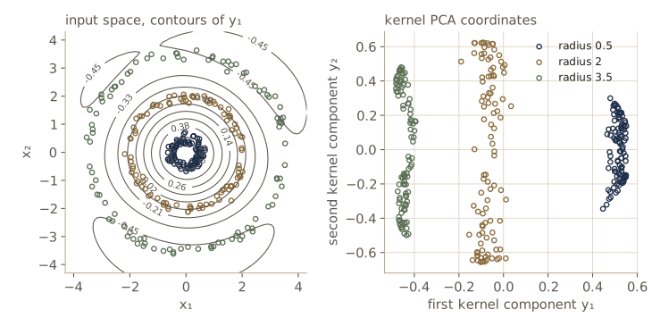
The width \(s\) of the kernel matters. Much smaller widths make the components describe local wiggles of single rings, and much larger ones make the kernel nearly quadratic, so the components become smooth functions that no longer follow the rings; one way to choose it is to try several widths, as with any kernel method.
The pre-image problem
Linear PCA can reconstruct a data point from its \(M\) coordinates, as we did for the bar images. Kernel PCA cannot do this directly. Its reconstruction \(\sum_i y_i\mathbf{v}_i\) is a point in feature space, and in general no input \(\mathbf{x}\) has exactly that feature vector: the image of the input space is a curved surface inside the feature space, and the reconstruction usually lies off it. Finding an input whose feature vector is close to a given feature-space point is the pre-image problem. It has approximate solutions (for the Gaussian kernel, a fixed-point iteration; more generally, a small optimization), and it matters for applications such as denoising, where the reconstruction is the goal. Bishop §12.3 gives references.
Nonlinear latent variable models
PPCA and factor analysis are linear and Gaussian. That makes them easy to fit and to analyze, but real data can be non-Gaussian, curved, or both. The two issues are related: any well-behaved density can be produced by passing a Gaussian variable through a suitable nonlinear function (Bishop Exercise 12.28). This section sketches three ways to go beyond the linear-Gaussian case: keep the map linear but make the latent distribution non-Gaussian (independent component analysis), learn a nonlinear map with a neural network (autoencoders), and a family of other nonlinear manifold methods.
Independent component analysis
Two people talk at once in a room with two microphones. Ignoring delays and echoes, each microphone records a fixed linear combination of the two voices. From the two recordings alone, without knowing the voices or the mixing coefficients, can we recover the voices? This is blind source separation.
Independent component analysis (ICA) models it as a latent variable model with a linear map, no noise, as many latent variables as observed ones, and a factorized latent distribution:
\[\mathbf{x} = \mathbf{A}\mathbf{z}, \qquad p(\mathbf{z}) = \prod_{j=1}^{M} p(z_j).\]Here the \(z_j\) are the sources and \(\mathbf{A}\) is the \(M \times M\) mixing matrix. We treat successive samples as independent draws and ignore their order in time. If \(\mathbf{W} = \mathbf{A}^{-1}\) is the unmixing matrix with rows \(\mathbf{w}_j^{\mathrm{T}}\), the change-of-variables formula gives
\[p(\mathbf{x}) = \lvert \det\mathbf{W} \rvert \prod_{j=1}^{M} p_j(\mathbf{w}_j^{\mathrm{T}}\mathbf{x}),\]so the log-likelihood of \(N\) observations is
\[\ln p(\mathbf{X}) = N\ln\lvert \det\mathbf{W} \rvert + \sum_{n=1}^{N}\sum_{j=1}^{M}\ln p_j(\mathbf{w}_j^{\mathrm{T}}\mathbf{x}_n),\]and we can fit \(\mathbf{W}\) by maximizing this log-likelihood with gradient methods. Bishop’s example of a source density, taken from MacKay, is \(p(z) = 1/(\pi\cosh z)\), which has heavier tails than a Gaussian, like speech.
Watch out. The sources must not be Gaussian. If \(p(\mathbf{z})\) is a standard Gaussian, then \(\mathbf{A}\mathbf{z}\) and \(\mathbf{A}\mathbf{R}\mathbf{z}\) have the same distribution for every orthogonal \(\mathbf{R}\), the rotational ambiguity of PPCA again, and no amount of data can tell the true mixing matrix from a rotated one. Decorrelating the data, as PCA does, removes only part of the mixing: uncorrelated is not the same as independent (Bishop Exercise 12.29).
Whitening first. After whitening the data (\(\mathbf{x} \mapsto \mathbf{L}^{-1/2}\mathbf{U}^{\mathrm{T}}(\mathbf{x} - \bar{\mathbf{x}})\)), and scaling the sources to unit variance, the remaining unmixing matrix must be orthogonal: both the whitened data and the sources have identity covariance. So ICA reduces to finding a rotation, and \(\ln\lvert\det\mathbf{W}\rvert = 0\) along the way.
FastICA. A popular algorithm, due to Hyvärinen and Oja, searches for the rotation that makes each output as non-Gaussian as possible. It measures non-Gaussianity of \(y = \mathbf{w}^{\mathrm{T}}\mathbf{x}\) through \(\mathbb{E}[G(y)]\) for a smooth contrast function, here \(G(y) = \ln\cosh y\) with derivative \(g(y) = \tanh y\). With \(\lVert\mathbf{w}\rVert = 1\) enforced, a Newton step on this objective simplifies to the fixed-point update
\[\mathbf{w} \leftarrow \mathbb{E}\left[\mathbf{x}\,g(\mathbf{w}^{\mathrm{T}}\mathbf{x})\right] - \mathbb{E}\left[g'(\mathbf{w}^{\mathrm{T}}\mathbf{x})\right]\mathbf{w},\]followed by renormalization. The symmetric version updates all rows of \(\mathbf{W}\) at once and then makes them orthonormal again with \(\mathbf{W} \leftarrow (\mathbf{W}\mathbf{W}^{\mathrm{T}})^{-1/2}\mathbf{W}\), which we compute from an SVD. Note the link with the likelihood: with the \(1/\cosh\) source density, \(\ln p(z) = -\ln\cosh z\) plus a constant, so for whitened data the ICA log-likelihood is \(-N\,\mathbb{E}[\ln\cosh y]\) summed over outputs, the same contrast function.
Our two sources are a sine wave and a sawtooth, both non-Gaussian, mixed by a fixed matrix.
t = np.linspace(0, 8, 2000)
sources = np.column_stack([np.sin(2 * np.pi * t),       # sine
                           2 * ((1.7 * t) % 1) - 1])      # sawtooth
sources = (sources - sources.mean(0)) / sources.std(0)
A_mix = np.array([[1.0, 0.6], [0.5, 1.0]])
X_mix = sources @ A_mix.T

def excess_kurtosis(y):
    y = (y - y.mean()) / y.std()
    return np.mean(y ** 4) - 3.0

def fastica(Xw, n_iter, rng, tol=1e-10):
    """Symmetric FastICA with G = ln cosh on whitened data.
    The rows of the result are the unmixing directions."""
    N, D = Xw.shape
    W = np.linalg.qr(rng.standard_normal((D, D)))[0]
    for it in range(1, n_iter + 1):
        Y = Xw @ W.T
        g, g_prime = np.tanh(Y), 1 - np.tanh(Y) ** 2
        W_new = g.T @ Xw / N - g_prime.mean(axis=0)[:, None] * W   # fixed-point update
        u, _, vt = np.linalg.svd(W_new)
        W_new = u @ vt                                              # (W W^T)^{-1/2} W
        change = np.max(np.abs(np.abs(np.sum(W_new * W, axis=1)) - 1))
        W = W_new
        if change < tol:
            break
    print(f"FastICA converged after {it} iterations")
    return W

Xw_mix, _, lam_mix, U_mix = whiten(X_mix)
W_ica = fastica(Xw_mix, 200, np.random.default_rng(0))
Y_ica = Xw_mix @ W_ica.T

print("excess kurtosis, sources: ", [f"{excess_kurtosis(s):+.3f}" for s in sources.T])
print("excess kurtosis, mixtures:", [f"{excess_kurtosis(x):+.3f}" for x in X_mix.T])
print("correlations (rows: outputs, columns: true sources)")
for name, Y in [("whitening only", Xw_mix), ("FastICA", Y_ica)]:
    print(f"  {name:15s}", np.round(np.corrcoef(Y.T, sources.T)[:2, 2:], 3).tolist())
FastICA converged after 6 iterations
excess kurtosis, sources:  ['-1.499', '-1.184']
excess kurtosis, mixtures: ['-0.924', '-0.860']
correlations (rows: outputs, columns: true sources)
  whitening only  [[-0.693, -0.728], [0.721, -0.686]]
  FastICA         [[0.013, 1.0], [1.0, -0.004]]
After FastICA, each output correlates almost perfectly with one source and hardly at all with the other. Whitening alone produces uncorrelated outputs that are still mixtures. Notice also the kurtosis values: mixing pushed both signals toward Gaussian (excess kurtosis closer to 0), a consequence of the central limit theorem, and unmixing moves them back. Which source comes out first, and with which sign and scale, is arbitrary; those three ambiguities (order, sign, scale) are inherent in the model, since \(\mathbf{A}\) and \(\mathbf{z}\) can trade any of them.
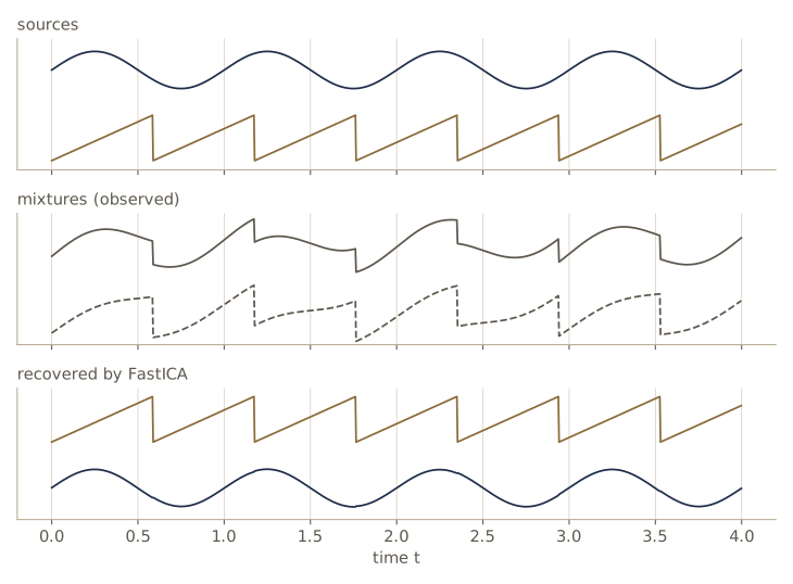
Since the whitened problem is only a rotation, we can see all of this by brute force over the rotation angle: measure the total non-Gaussianity of the two outputs, and also evaluate the ICA log-likelihood under the \(1/\cosh\) source density.
def rotation(a):
    return np.array([[np.cos(a), np.sin(a)], [-np.sin(a), np.cos(a)]])

def total_abs_kurtosis(Y):
    return sum(abs(excess_kurtosis(y)) for y in Y.T)

def loglik_cosh(Y):
    """Mean over samples of sum_j ln p(y_j) with p(y) = 1 / (pi cosh y)."""
    return np.mean(np.sum(-np.log(np.pi * np.cosh(Y)), axis=1))

deg = np.arange(0, 90, 0.5)
nongauss = [total_abs_kurtosis(Xw_mix @ rotation(np.radians(a)).T) for a in deg]
ll_cosh = [loglik_cosh(Xw_mix @ rotation(np.radians(a)).T) for a in deg]
a_fast = np.degrees(np.arctan2(W_ica[0, 1], W_ica[0, 0])) % 90
print(f"FastICA rotation angle (mod 90): {a_fast:.2f} deg")
print(f"largest total abs(excess kurtosis) at {deg[np.argmax(nongauss)]:.1f} deg")
print(f"1/cosh log-likelihood: maximum at {deg[np.argmax(ll_cosh)]:.1f} deg, "
      f"minimum at {deg[np.argmin(ll_cosh)]:.1f} deg")

gauss_src = np.random.default_rng(8).standard_normal((2000, 2))
Xw_g, *_ = whiten(gauss_src @ A_mix.T)
ng = [total_abs_kurtosis(Xw_g @ rotation(np.radians(a)).T) for a in deg]
print(f"Gaussian sources: total abs(excess kurtosis) {min(ng):.3f} to {max(ng):.3f}")
FastICA rotation angle (mod 90): 43.11 deg
largest total abs(excess kurtosis) at 43.0 deg
1/cosh log-likelihood: maximum at 88.0 deg, minimum at 43.0 deg
Gaussian sources: total abs(excess kurtosis) 0.059 to 0.184
Three lessons. The rotation found by FastICA sits where the outputs are most non-Gaussian. For Gaussian sources the non-Gaussianity is small at every angle (it is only sampling noise), so there is nothing to find. And the maximum likelihood approach with the heavy-tailed \(1/\cosh\) density gets this data set exactly wrong: its log-likelihood is lowest at the separating rotation and highest 45 degrees away. Our sources are light-tailed (negative excess kurtosis), and a heavy-tailed source model prefers mixtures, which have heavier tails than these sources. FastICA avoids the trap because it looks for extremes of \(\mathbb{E}[G(y)]\) in either direction; a likelihood approach must use a source density with the right kind of tails (Exercise 9 asks you to check the heavy-tailed case).
The original ICA algorithm of Bell and Sejnowski was derived from an information-maximization principle. The probabilistic view has the advantage of suggesting extensions, for instance models with noise, with fewer sources than sensors, or with source densities that are themselves mixtures of Gaussians (Bishop §12.4.1).
Autoassociative neural networks
In module 05 neural networks mapped inputs to targets. They can also reduce dimension: train a network to reproduce its own input through a narrow middle layer. A network with \(D\) inputs, \(M < D\) hidden units, and \(D\) outputs, trained so that the outputs match the inputs, is an autoassociative network or autoencoder. The error is the usual sum of squares,
\[E(\mathbf{w}) = \frac{1}{2}\sum_{n=1}^{N}\lVert \mathbf{y}(\mathbf{x}_n, \mathbf{w}) - \mathbf{x}_n \rVert^2 ,\]and because the middle layer is narrower than the input, the network cannot simply copy; it must find a compressed code.
With linear units, \(\mathbf{y}(\mathbf{x}) = \mathbf{W}_2\mathbf{W}_1\mathbf{x}\) for an encoder \(\mathbf{W}_1\) (\(M \times D\)) and a decoder \(\mathbf{W}_2\) (\(D \times M\)), where we work with centered data so that biases can be dropped. The product \(\mathbf{W}_2\mathbf{W}_1\) has rank at most \(M\), so the best it can do is the best rank-\(M\) approximation of the data, and the minimum-error argument from the PCA section says what that is: projection onto the principal subspace, with error \(\frac{N}{2}\sum_{i>M}\lambda_i\). It is known that this error function has no local minima other than the global one, only saddle points (Baldi and Hornik, 1989), so gradient descent should find it. We train one on the PPCA data set, averaging the error over the data. The gradients are \(\partial E/\partial\mathbf{W}_2 = \mathbf{R}^{\mathrm{T}}\mathbf{Z}\) and \(\partial E/\partial\mathbf{W}_1 = \mathbf{W}_2^{\mathrm{T}}\mathbf{R}^{\mathrm{T}}\tilde{\mathbf{X}}\), where \(\mathbf{Z} = \tilde{\mathbf{X}}\mathbf{W}_1^{\mathrm{T}}\) holds the hidden activations and \(\mathbf{R} = \mathbf{Z}\mathbf{W}_2^{\mathrm{T}} - \tilde{\mathbf{X}}\) the residuals; we check them with finite differences first.
def linear_ae_loss_grad(W1, W2, Xc):
    """Mean over n of (1/2) ||W2 W1 x_n - x_n||^2 and its gradients."""
    N = len(Xc)
    Z = Xc @ W1.T                       # hidden activations, N x M
    R = Z @ W2.T - Xc                   # residuals, N x D
    E = 0.5 * np.sum(R ** 2) / N
    return E, W2.T @ R.T @ Xc / N, R.T @ Z / N

Xc_p = X_p - X_p.mean(axis=0)
rng_ae = np.random.default_rng(1)
W1 = 0.1 * rng_ae.standard_normal((3, D_p))
W2 = 0.1 * rng_ae.standard_normal((D_p, 3))

_, g1, g2 = linear_ae_loss_grad(W1, W2, Xc_p)
theta_ae = np.concatenate([W1.ravel(), W2.ravel()])
def f_ae(th):
    W1_, W2_ = th[:30].reshape(3, D_p), th[30:].reshape(D_p, 3)
    return linear_ae_loss_grad(W1_, W2_, Xc_p)[0]

g_exact = np.concatenate([g1.ravel(), g2.ravel()])
g_num = num_grad(f_ae, theta_ae)
print(f"gradient check: max abs difference {np.abs(g_num - g_exact).max():.1e}")

eta = 0.01
for it in range(1, 3001):
    E, g1, g2 = linear_ae_loss_grad(W1, W2, Xc_p)
    W1 -= eta * g1
    W2 -= eta * g2
    if it in (1, 10, 100, 500, 1000, 3000):
        print(f"step {it:4d}: E = {E:9.6f}, angles to top-3 eigenvectors",
              principal_angles(W2, U_p[:, :3]))
print(f"(1/2) sum of the discarded eigenvalues = {0.5 * lam_p[3:].sum():.6f}")
print(f"W2^T W2:\n{W2.T @ W2}")
print("abs cosines, decoder columns (rows) vs u_1, u_2, u_3 (columns):")
print(np.abs((W2 / np.linalg.norm(W2, axis=0)).T @ U_p[:, :3]))
print(f"max abs(W1 - pinv(W2)) = {np.abs(W1 - np.linalg.pinv(W2)).max():.1e}")
gradient check: max abs difference 6.2e-10
step    1: E = 33.715603, angles to top-3 eigenvectors [32.8363 48.9728 87.8287]
step   10: E = 10.776308, angles to top-3 eigenvectors [ 3.0253 27.777  85.2721]
step  100: E =  2.871624, angles to top-3 eigenvectors [ 0.1034  0.719  23.9786]
step  500: E =  2.265742, angles to top-3 eigenvectors [0.0078 0.0689 0.5242]
step 1000: E =  2.264920, angles to top-3 eigenvectors [0.0003 0.005  0.037 ]
step 3000: E =  2.264915, angles to top-3 eigenvectors [0. 0. 0.]
(1/2) sum of the discarded eigenvalues = 2.264915
W2^T W2:
[[ 1.033  -0.0031  0.0345]
 [-0.0031  1.0444  0.0103]
 [ 0.0345  0.0103  0.9466]]
abs cosines, decoder columns (rows) vs u_1, u_2, u_3 (columns):
[[0.1904 0.9565 0.2209]
 [0.1221 0.2493 0.9607]
 [0.9813 0.1251 0.1464]]
max abs(W1 - pinv(W2)) = 2.6e-07
The trained network reaches the PCA error exactly, and the columns of the decoder span the principal subspace (all three principal angles go to zero). But the columns are not the individual eigenvectors: each is a mixture, with cosines of 0.96 to 0.98 with its nearest eigenvector. Any invertible \(M \times M\) matrix can be inserted between encoder and decoder without changing the product, so only the subspace is determined. (Here the columns happen to be nearly orthonormal, \(\mathbf{W}_2^{\mathrm{T}}\mathbf{W}_2 \approx \mathbf{I}\), because gradient descent from small random weights keeps the encoder close to the transpose of the decoder; from a different starting point they need not be.) At the optimum the encoder is the pseudo-inverse of the decoder, which maps each point to the coordinates of its orthogonal projection. Compared with an SVD, which gives the answer in one step together with an ordered set of orthonormal components, gradient descent is a slow route to PCA.
Making the hidden units of this two-layer network nonlinear does not help: the best achievable error is still that of projection onto the principal subspace (Bishop §12.4.2). Genuine nonlinear dimensionality reduction needs more layers. In a four-layer autoencoder, an input layer feeds a layer of nonlinear units, then the \(M\)-unit bottleneck, then another nonlinear layer, then the linear outputs. The first half is a nonlinear map \(\mathbf{F}_1\) from \(\mathbb{R}^D\) to \(\mathbb{R}^M\), the second a nonlinear map \(\mathbf{F}_2\) back, and \(\mathbf{F}_2\) describes a curved \(M\)-dimensional surface in data space onto which \(\mathbf{F}_1\) projects. This is a form of nonlinear PCA. The cost is a harder, nonconvex optimization with local minima, and \(M\) must be chosen in advance.
Deep autoencoders, trained with the methods of module 05 on large data sets, are the modern descendants of this idea, and variational autoencoders combine them with the latent variable view of this module: a nonlinear decoder plays the role of \(\mathbf{W}\mathbf{z} + \boldsymbol{\mu}\), and a second network approximates the posterior \(p(\mathbf{z} \mid \mathbf{x})\), using the variational ideas of module 10.
Modeling nonlinear manifolds
Many other methods try to capture curved low-dimensional structure. One line each, with the idea that sets it apart:
- Mixtures of PPCA. Approximate a curved manifold by flat pieces: a mixture model (module 09) whose components are PPCA models, fitted by EM with both discrete and continuous latent variables. Replacing isotropic noise by diagonal noise gives a mixture of factor analyzers.
- Principal curves. A smooth curve through the data such that each point of the curve is the average of the data points that project onto it; fitted by alternating projection and smoothing steps, starting from the first principal component. Principal surfaces extend the idea to more dimensions.
- Multidimensional scaling (MDS). Place points in a low-dimensional space so that their pairwise distances match given distances as closely as possible; for Euclidean distances classical MDS gives the same result as PCA.
- Isomap. Classical MDS applied to geodesic distances, estimated as shortest paths through a nearest-neighbor graph, so that distances are measured along the manifold rather than through the space around it.
- Locally linear embedding (LLE). Describe each point as a weighted combination of its neighbors, then find low-dimensional points that are reconstructed by the same weights; the optimization is an eigenproblem without local minima.
- Latent trait models and density networks. Continuous latent variables with discrete observations, or with a neural-network map from latent to data space; the marginal likelihood is no longer tractable and must be approximated, for instance by sampling.
- Generative topographic mapping (GTM). A density network made tractable: the latent space is a regular grid of points, and the map is a linear combination of fixed basis functions, so EM applies.
- Self-organizing map (SOM). A grid of prototype vectors that are pulled toward the data while neighboring prototypes are kept similar; GTM was developed as a probabilistic counterpart of it.
In practice. Try PCA first. It is fast, it has no tuning parameters beyond \(M\), its eigenvalue spectrum tells you how much structure there is, and it is the standard preprocessing step before other methods. Reach for kernel PCA, manifold learners, or autoencoders when the spectrum shows that a flat subspace needs far more dimensions than you believe the data really have, as it did for the bar images.
Summary
| Model | Latent variables and map | Noise | How it is fit |
|---|---|---|---|
| PCA | \(M\) coordinates, orthogonal projection | none | eigenvectors of \(\mathbf{S}\) (or SVD of the centered data) |
| Probabilistic PCA | \(\mathbf{z} \sim \mathcal{N}(\mathbf{0}, \mathbf{I})\), \(\mathbf{x} = \mathbf{W}\mathbf{z} + \boldsymbol{\mu} + \boldsymbol{\epsilon}\) | isotropic, \(\sigma^2\mathbf{I}\) | closed form from the eigenvectors, or EM |
| Bayesian PCA | as PPCA, with an ARD prior on the columns of \(\mathbf{W}\) | isotropic | EM with re-estimated \(\alpha_i = D / \mathbf{w}_i^{\mathrm{T}}\mathbf{w}_i\) |
| Factor analysis | as PPCA | diagonal \(\boldsymbol{\Psi}\) | EM (no closed form) |
| Kernel PCA | linear PCA in a feature space | none | eigenvectors of the centered Gram matrix |
| ICA | \(\mathbf{x} = \mathbf{A}\mathbf{z}\), independent non-Gaussian \(z_j\) | none | whitening + FastICA, or maximum likelihood |
| Linear autoencoder | \(\mathbf{y} = \mathbf{W}_2\mathbf{W}_1\mathbf{x}\) | none (sum of squares) | gradient descent; finds the principal subspace |
Ideas to carry forward:
- PCA’s two definitions, maximum variance and minimum reconstruction error, are the same because the total variance is fixed. The error of keeping \(M\) components is the sum of the eigenvalues you discard.
- A latent variable model turns a geometric recipe into a density with a likelihood. For PPCA this buys maximum likelihood fitting, EM, principled model comparison, Bayesian dimension selection, and extensions such as mixtures and missing data.
- Gaussian latent variables come with a rotational ambiguity: only the subspace is identified. Compare subspaces with principal angles, not column by column. Breaking the ambiguity needs non-Gaussian latents, which is exactly what ICA exploits.
- Linear methods describe curved manifolds poorly; kernels, nonlinear networks, and neighborhood-graph methods are the main ways to go further.
Exercises
- Complete the induction behind the maximum-variance result: assume the variance-maximizing \(M\)-dimensional projection is spanned by \(\mathbf{u}_1, \dots, \mathbf{u}_M\), and show that the best additional direction orthogonal to all of them is \(\mathbf{u}_{M+1}\). Where do you use that \(\mathbf{S}\) is symmetric?
- Show that \(\frac{1}{N}\sum_n \lVert \mathbf{x}_n - \bar{\mathbf{x}} \rVert^2 = \operatorname{Tr}(\mathbf{S}) = \sum_i\lambda_i\), and use it to explain in two lines why maximizing the projected variance and minimizing the distortion \(J\) give the same subspace. Then verify numerically, for the bar images and \(M = 5\), that captured variance plus distortion equals the total variance.
- PCA through the SVD. Let \(\tilde{\mathbf{X}} = \mathbf{P}\boldsymbol{\Sigma}\mathbf{Q}^{\mathrm{T}}\) be the thin SVD of the centered data matrix. Show that the columns of \(\mathbf{Q}\) are eigenvectors of \(\mathbf{S}\) with eigenvalues \(\sigma_i^2/N\), and that \(\mathbf{P}\boldsymbol{\Sigma}\) contains the principal coordinates. Write
pca_svd(X)and check it againstpcaon the bar images. - Implement the power method for the first principal component of the bar images: start from a random unit vector, multiply by \(\mathbf{S}\), and renormalize. How many iterations are needed for an angle below \(10^{-3}\) degrees to \(\mathbf{u}_1\)? Relate the answer to \(\lambda_2/\lambda_1\). Then extend it to \(M\) components by orthogonalizing a block of vectors after each multiplication (subspace iteration).
- For PPCA, show that the posterior mean \(\mathbf{M}^{-1}\mathbf{W}^{\mathrm{T}}(\mathbf{x} - \bar{\mathbf{x}})\) tends to \((\mathbf{W}^{\mathrm{T}}\mathbf{W})^{-1}\mathbf{W}^{\mathrm{T}}(\mathbf{x} - \bar{\mathbf{x}})\) as \(\sigma^2 \to 0\), and that \(\mathbf{W}\) times this limit is the orthogonal projection of \(\mathbf{x} - \bar{\mathbf{x}}\) onto the column space of \(\mathbf{W}\). For \(\sigma^2 > 0\), show that the reconstruction \(\mathbf{W}\,\mathbb{E}[\mathbf{z} \mid \mathbf{x}]\) is shorter than the orthogonal projection.
- Verify the PPCA parameter count: show that \(DM + 1 - M(M-1)/2\) equals \(D(D+1)/2\) (the count for a full covariance) when \(M = D - 1\), and equals 1 (an isotropic covariance) when \(M = 0\). Why is the case \(M = D\) not included?
- Derive the M-step update for \(\mathbf{W}\) in PPCA from the expected complete-data log-likelihood, and then the update for \(\sigma^2\). Modify
ppca_emto handle missing values: mark 20% of the entries ofX_pas missing at random, treat them as latent, and compare the recovered subspace with the one from complete data. - Factor analysis and rescaling. Multiply the first column of
X_faby 10. Fit factor analysis and PPCA again. Show that the factor analysis loadings and uniquenesses change exactly as the rescaling predicts (first row of \(\mathbf{W}\) times 10, first \(\psi\) times 100), while the PPCA solution changes in a qualitatively different way. - Replace the sine and sawtooth in the ICA experiment by two heavy-tailed sources (for instance, Laplace-distributed samples). Recompute the angle sweep. Where is the maximum of the \(1/\cosh\) log-likelihood now, and does it agree with FastICA? Then implement maximum likelihood ICA directly by gradient ascent on \(N\ln\lvert\det\mathbf{W}\rvert - \sum_{n,j}\ln\cosh(\mathbf{w}_j^{\mathrm{T}}\mathbf{x}_n)\) on the unwhitened mixtures, and check that it recovers the sources.
- Kernel PCA width. Rerun the ring experiment with \(s = 0.3\) and \(s = 5\), and describe what the first two components capture in each case. For a grid of widths, count the pairs of rings whose ranges on the first component overlap, and report the widths for which none do.
- Train the linear autoencoder on the bar images with \(M = 5\) and compare its final error with \(\frac{1}{2}\sum_{i>5}\lambda_i\). How does the number of gradient steps needed compare with the zero-noise EM algorithm on the same problem?
- In your own words: explain to a classmate what the rotational ambiguity of PPCA is, why it does no harm when all you want is the principal subspace, and why it is the reason ICA needs non-Gaussian sources.
Going further
- C. M. Bishop, Pattern Recognition and Machine Learning, chapter 12 — the source for this module. Exercises 12.1–12.3 cover the PCA derivations, 12.7–12.12 the PPCA marginal, posterior, and projection, 12.14–12.17 parameter counting, EM, and missing data, 12.18–12.22 and 12.25 factor analysis and its invariances, 12.26–12.27 kernel PCA, and 12.28–12.29 the ideas behind ICA.
- Michael E. Tipping and Christopher M. Bishop, “Probabilistic principal component analysis”, Journal of the Royal Statistical Society, Series B, 1999 — the maximum likelihood solution, EM, and mixtures of PPCA in full.
- Bernhard Schölkopf, Alexander Smola, and Klaus-Robert Müller, “Nonlinear component analysis as a kernel eigenvalue problem”, Neural Computation, 1998 — the paper that introduced kernel PCA.
- Aapo Hyvärinen and Erkki Oja, “Independent component analysis: algorithms and applications”, Neural Networks, 2000 — a readable tutorial on ICA and the FastICA algorithm.
- Sam Roweis, “EM algorithms for PCA and SPCA”, Advances in Neural Information Processing Systems 10, 1998 — the zero-noise EM algorithm for PCA.
- I. T. Jolliffe, Principal Component Analysis, 2nd edition, Springer, 2002 — a comprehensive book on PCA and its many uses.
These notes follow the chapters of C. M. Bishop, Pattern Recognition and Machine Learning (Springer, 2006), the course text, which Microsoft Research makes freely available as a PDF. The explanations, code, figures, and exercises here are written for this course; the book remains the reference, with the full derivations and many more exercises.