CSE 474/574 · Module 11 · Week 12
Sampling Methods
Transformation, rejection, and importance sampling; Markov chains, Metropolis–Hastings, Gibbs and slice sampling; Hamiltonian Monte Carlo.
Companion reading: Bishop, Pattern Recognition and Machine Learning, chapter 11, “Sampling Methods”
By the end of this module you can
- Estimate an expectation by Monte Carlo, derive the variance of the estimate, and explain why its accuracy depends on the number of independent samples and not on the dimension.
- Compute the effective sample size of a correlated sequence from its autocorrelations, and use it to compare samplers.
- Generate samples from standard distributions by inverting a CDF, by the Box–Muller method, and by a Cholesky factor, and check them against the exact distribution.
- Implement rejection sampling, importance sampling, and sampling-importance-resampling, predict the acceptance rate of a rejection sampler, and recognize when a poor proposal makes importance sampling silently wrong.
- Define invariant distributions, detailed balance, and ergodicity for a Markov chain, and prove that the Metropolis–Hastings and Gibbs updates leave the target distribution invariant.
- Run random-walk Metropolis, Gibbs sampling, and over-relaxed Gibbs sampling on a strongly correlated Gaussian and explain the random-walk cost of order \((\sigma_{\max}/\sigma_{\min})^2\) steps.
- Implement slice sampling with stepping out and shrinkage, and Hamiltonian Monte Carlo with leapfrog integration and a Metropolis correction.
- Estimate a ratio of normalizing constants by importance sampling and explain why it degrades when the two distributions are poorly matched.
Contents
- Monte Carlo estimates of expectations
- Basic sampling algorithms
- Markov chain Monte Carlo
- Gibbs sampling
- Slice sampling
- Hybrid Monte Carlo
- Estimating the partition function
- Summary
- Exercises
- Going further
In module 10 we met models whose posterior distributions cannot be computed exactly, and we replaced them with simpler distributions fitted by optimization: variational inference and expectation propagation. Those methods are fast, but they are approximations by design, and the approximation does not go away no matter how much computer time we spend.
This module takes the other road. Instead of approximating the distribution with a formula, we draw samples from it and use them to estimate whatever we need. The methods go by the name Monte Carlo. Their appeal is that, given enough time, they become exact. Their difficulty is that “enough time” can be very long, and much of the module is about why, and about how clever samplers shorten it.
We start with the Monte Carlo estimate itself and its error. Then we build samplers in order of generality: exact recipes for standard distributions, rejection and importance sampling (which work well in one or two dimensions), and Markov chain Monte Carlo (Metropolis–Hastings, Gibbs sampling, slice sampling, and Hamiltonian Monte Carlo), which is how most Bayesian computation in high dimensions is done. The graphical models of module 08, the EM algorithm of module 09, and the Gaussian identities of module 02 all reappear.
Monte Carlo estimates of expectations
The basic estimator
Most of what we want from a posterior distribution is an expectation. A predictive distribution, a posterior mean, the probability of an event: each has the form
\[\mathbb{E}[f] = \int f(\mathbf{z})\, p(\mathbf{z})\, d\mathbf{z},\]with a sum in place of the integral for discrete \(\mathbf{z}\). Suppose we can draw independent samples \(\mathbf{z}^{(1)}, \dots, \mathbf{z}^{(L)}\) from \(p(\mathbf{z})\). The Monte Carlo estimate of the expectation is the sample average
\[\widehat{f} = \frac{1}{L} \sum_{l=1}^{L} f(\mathbf{z}^{(l)}).\]Its properties follow from the linearity of expectation. Each term has mean \(\mathbb{E}[f]\), so \(\mathbb{E}[\widehat{f}] = \mathbb{E}[f]\): the estimate is unbiased. Because the terms are independent, the variance of the sum is the sum of the variances, and
\[\operatorname{var}[\widehat{f}] = \frac{1}{L^2} \sum_{l=1}^{L} \operatorname{var}[f(\mathbf{z}^{(l)})] = \frac{1}{L}\, \operatorname{var}[f], \qquad \operatorname{var}[f] = \mathbb{E}\big[(f - \mathbb{E}[f])^2\big].\]The standard error falls like \(1/\sqrt{L}\): a hundred times more samples buys one more correct digit. That is slow compared with a numerical quadrature rule in one dimension. But notice what the formula does not contain. The dimension of \(\mathbf{z}\) appears nowhere. Only the variance of the function \(f\) matters.
Accuracy does not depend on dimension
Let us check this. We estimate the probability that a standard Gaussian vector in \(D\) dimensions satisfies \(\lVert \mathbf{z} \rVert^2 < D\), so \(f\) is an indicator function and \(\operatorname{var}[f] = p(1-p)\) where \(p\) is the probability. The exact answer comes from the chi-squared distribution (we use scipy.stats only as a check). We repeat the whole estimate 100 times for each setting and measure how much the estimates spread.
import math
import numpy as np
from scipy import stats
from scipy.special import logsumexp, gammaln

np.set_printoptions(precision=4, suppress=True)
rng = np.random.default_rng(11)
R = 100                                            # independent repetitions of the estimate
print("   D  p (exact)   sd, L=100  theory   sd, L=1000  theory")
for D in [1, 10, 100, 1000]:
    p = stats.chi2.cdf(D, df=D)                    # exact P(||z||^2 < D), for checking
    line = f"{D:4d}   {p:.4f}"
    for L in [100, 1000]:
        est = np.array([np.mean(np.sum(rng.standard_normal((L, D))**2, axis=1) < D)
                        for _ in range(R)])
        line += f"    {est.std():.4f}    {np.sqrt(p * (1 - p) / L):.4f}"
    print(line)
   D  p (exact)   sd, L=100  theory   sd, L=1000  theory
   1   0.6827    0.0478    0.0465    0.0127    0.0147
  10   0.5595    0.0489    0.0496    0.0169    0.0157
 100   0.5188    0.0483    0.0500    0.0154    0.0158
1000   0.5059    0.0517    0.0500    0.0184    0.0158
With 100 samples the estimates scatter by about 0.05 whether \(\mathbf{z}\) has one component or a thousand; with 1000 samples, by about 0.015, which is \(\sqrt{10}\) times less. The measured spreads agree with \(\sqrt{p(1-p)/L}\) to within the noise of using 100 repetitions. Compare a grid: ten points per axis would need \(10^{1000}\) evaluations of the integrand in the last row.
Note. The dimension-free error bar is the reason sampling is the method of choice for high-dimensional integrals. The catch is in the assumption: the samples must come from \(p(\mathbf{z})\) itself, and independently. Drawing such samples is the hard part, and the rest of this module is about it. A second, quieter catch: if \(f\) is large only where \(p\) is small, then \(\operatorname{var}[f]\) is large relative to \(\mathbb{E}[f]^2\), and many samples are needed before any of them land where \(f\) matters.
Correlated samples and the effective sample size
Many samplers in this module produce a sequence in which each sample depends on the previous one. The average is still a sensible estimate, but the variance formula changes. Suppose the sequence is stationary with variance \(\sigma^2 = \operatorname{var}[f]\) and autocorrelation \(\rho_k = \operatorname{cov}[f_l, f_{l+k}] / \sigma^2\) at lag \(k\), where \(f_l = f(\mathbf{z}^{(l)})\). The variance of the sum now includes all the covariances:
\[\operatorname{var}[\widehat{f}] = \frac{1}{L^2} \sum_{l=1}^{L} \sum_{m=1}^{L} \operatorname{cov}[f_l, f_m] = \frac{\sigma^2}{L} \Big(1 + 2 \sum_{k=1}^{L-1} \big(1 - \tfrac{k}{L}\big) \rho_k \Big) \approx \frac{\sigma^2}{L}\, \tau,\]where the last step assumes the correlations die out long before lag \(L\). The number
\[\tau = 1 + 2 \sum_{k=1}^{\infty} \rho_k\]is the integrated autocorrelation time. The correlated sequence of length \(L\) gives the same accuracy as \(L/\tau\) independent samples, and we call \(L/\tau\) the effective sample size (ESS).
To estimate \(\tau\) from a finite run we compute the sample autocorrelations and add them up, but the estimates at large lags are pure noise, so we must stop somewhere. A standard rule, due to Geyer, adds the autocorrelations in adjacent pairs \(\rho_{2m} + \rho_{2m+1}\) and stops at the first pair that is not positive (for a reversible chain the true pair sums are positive and decreasing). We will use these functions for every sampler in the module.
def autocorr(x, max_lag):
    """Sample autocorrelation of a 1-D series at lags 0..max_lag (FFT, zero-padded)."""
    x = np.asarray(x, float) - np.mean(x)
    n = len(x)
    F = np.fft.rfft(x, 2 * n)
    acov = np.fft.irfft(F * np.conj(F))[: max_lag + 1] / n
    return acov / acov[0]

def iat(x):
    """Integrated autocorrelation time tau = 1 + 2 sum_k rho_k, summing pairs
    rho_2m + rho_2m+1 until the first pair that is not positive."""
    rho = autocorr(x, len(x) - 1)
    pairs = rho[: 2 * (len(rho) // 2)].reshape(-1, 2).sum(axis=1)
    stop = np.argmax(pairs <= 0) if np.any(pairs <= 0) else len(pairs)
    return max(1.0, -1.0 + 2.0 * pairs[:stop].sum())   # rho_0 = 1 is counted in pairs[0]

def ess(x):
    """Effective sample size L / tau."""
    return len(x) / iat(x)
A good test case is the autoregressive sequence \(z_l = \rho z_{l-1} + \sqrt{1 - \rho^2}\, \epsilon_l\) with \(\epsilon_l \sim \mathcal{N}(0, 1)\). Every \(z_l\) is a standard Gaussian, and the lag-\(k\) autocorrelation is \(\rho^k\), so a geometric series gives \(\tau = 1 + 2\rho/(1-\rho) = (1+\rho)/(1-\rho)\). We run 200 such sequences at once and compare the variance of their means with the independent-sample value \(1/L\).
def ar1_chains(rho, L, C, rng):
    """C independent AR(1) sequences of length L with N(0, 1) marginals; shape (L, C)."""
    z = np.empty((L, C))
    z[0] = rng.standard_normal(C)
    noise = np.sqrt(1 - rho**2) * rng.standard_normal((L, C))
    for t in range(1, L):
        z[t] = rho * z[t - 1] + noise[t]
    return z

rho, L, C = 0.9, 10_000, 200
z = ar1_chains(rho, L, C, rng)
means = z.mean(axis=0)
print(f"var of the mean, correlated:  {means.var():.2e}")
print(f"var of the mean, independent: {1 / L:.2e}")
print(f"ratio {means.var() * L:.1f};  theory tau = (1 + rho)/(1 - rho) = {(1 + rho) / (1 - rho):.1f}")
print(f"tau estimated from one sequence: {iat(z[:, 0]):.1f};  ESS = {ess(z[:, 0]):.0f} of {L}")
var of the mean, correlated:  1.81e-03
var of the mean, independent: 1.00e-04
ratio 18.1;  theory tau = (1 + rho)/(1 - rho) = 19.0
tau estimated from one sequence: 22.7;  ESS = 440 of 10000
With \(\rho = 0.9\) the 10,000 correlated values are worth only about 500 independent ones. The variance ratio measured across the 200 sequences (18.1) and the estimate of \(\tau\) from a single sequence (22.7) both sit near the exact 19; single-run estimates of \(\tau\) are themselves noisy, which is worth remembering when we compare samplers later.
Sampling from a directed graphical model
For a directed graphical model (module 08) with no observed variables, drawing an exact sample is easy. The joint distribution factorizes as \(p(\mathbf{z}) = \prod_i p(\mathbf{z}_i \mid \mathrm{pa}_i)\), so we visit the nodes in an order where parents come before children and sample each node from its conditional distribution given the values already drawn for its parents. This is ancestral sampling. To sample a marginal, such as \(p(\mathbf{u})\) from a joint \(p(\mathbf{u}, \mathbf{v})\), we draw from the joint and ignore \(\mathbf{v}\).
Observed variables complicate things. The simplest fix, logic sampling, runs ancestral sampling and throws away every sample whose values disagree with the observations. What survives is an exact sample from the posterior, but the fraction that survives is the probability of the evidence, which shrinks quickly as more variables are observed. A second option, previewed here and explained in the importance-sampling section below, is to clamp the observed nodes and weight each sample instead of discarding it.
Here is a four-node network: a cloudy day \(C\) influences whether a sprinkler runs (\(S\)) and whether it rains (\(R\)), and both affect whether the grass is wet (\(W\)). We ask for \(p(R = 1 \mid W = 1)\), first exactly by summing the joint, then by logic sampling.
pC = 0.4                                   # p(C = 1)
pS = {1: 0.1, 0: 0.6}                      # p(S = 1 | C)
pR = {1: 0.7, 0: 0.1}                      # p(R = 1 | C)
pW = {(1, 1): 0.95, (1, 0): 0.85, (0, 1): 0.80, (0, 0): 0.02}   # p(W = 1 | S, R)

def joint(c, s, r, w):
    """p(C, S, R, W) from the four conditional tables."""
    pc = pC if c else 1 - pC
    ps = pS[c] if s else 1 - pS[c]
    pr = pR[c] if r else 1 - pR[c]
    pw = pW[(s, r)] if w else 1 - pW[(s, r)]
    return pc * ps * pr * pw

states = [(c, s, r) for c in (0, 1) for s in (0, 1) for r in (0, 1)]
p_W1 = sum(joint(c, s, r, 1) for c, s, r in states)
exact = sum(joint(c, s, r, 1) for c, s, r in states if r == 1) / p_W1
print(f"exact p(R=1 | W=1) = {exact:.4f}    p(W=1) = {p_W1:.4f}")

def p_wet(s, r):
    """p(W = 1 | S, R) for boolean arrays s, r."""
    return np.select([s & r, s & ~r, ~s & r], [pW[(1, 1)], pW[(1, 0)], pW[(0, 1)]], pW[(0, 0)])

def ancestral(n, rng):
    """n joint samples, parents before children."""
    c = rng.random(n) < pC
    s = rng.random(n) < np.where(c, pS[1], pS[0])
    r = rng.random(n) < np.where(c, pR[1], pR[0])
    w = rng.random(n) < p_wet(s, r)
    return c, s, r, w

n_bn = 20_000
c, s, r, w = ancestral(n_bn, rng)
print(f"logic sampling: kept {w.sum()} of {n_bn};  p(R=1 | W=1) ~ {r[w].mean():.4f}")
exact p(R=1 | W=1) = 0.4909    p(W=1) = 0.5737
logic sampling: kept 11543 of 20000;  p(R=1 | W=1) ~ 0.5035
About 58% of the samples agree with \(W = 1\), matching \(p(W = 1)\), and the survivors give an estimate about 0.01 from the exact posterior probability. With ten observed variables the survival rate would be the product of many such probabilities, and logic sampling would waste nearly all its work.
Basic sampling algorithms
A computer generates pseudo-random numbers: a deterministic sequence that passes statistical tests for randomness. We take for granted a good generator of numbers uniform on \((0, 1)\); NumPy’s default_rng supplies one, and seeding it makes every result in these notes repeatable. The question of this section is how to turn uniform numbers into samples from other distributions.
Standard distributions: the transformation method
If \(z\) is uniform on \((0, 1)\) and \(y = g(z)\) for an increasing function \(g\), the change-of-variables rule gives \(p(y) = p(z)\, \lvert dz/dy \rvert = dz/dy\). We want to choose \(g\) so that \(p(y)\) is a given density. Integrating \(dz/dy = p(y)\) says that \(z = h(y)\), where
\[h(y) = \int_{-\infty}^{y} p(\widehat{y})\, d\widehat{y}\]is the cumulative distribution function (CDF) of the target. So \(y = h^{-1}(z)\): to sample from a distribution, feed uniform numbers through the inverse of its CDF. This is the transformation method, also called inverse-CDF sampling.
Two examples where \(h\) can be inverted by hand:
- The exponential distribution \(p(y) = \lambda e^{-\lambda y}\) for \(y \ge 0\) has \(h(y) = 1 - e^{-\lambda y}\), so \(y = -\lambda^{-1} \ln(1 - z)\).
- The Cauchy distribution \(p(y) = \frac{1}{\pi}\frac{1}{1 + y^2}\) has \(h(y) = \frac{1}{2} + \frac{1}{\pi}\arctan y\), so \(y = \tan\big(\pi (z - \tfrac{1}{2})\big)\). A location \(c\) and scale \(s\) give \(c + s \tan(\cdot)\).
We check each sampler against the exact distribution from scipy.stats, with sample moments and a Kolmogorov–Smirnov (KS) test, whose p-value should look like a uniform random number when the sampler is right and be tiny when it is wrong.
def sample_exponential(lam, L, rng):
    """Inverse CDF: y = -ln(1 - z) / lam with z ~ U(0, 1)."""
    return -np.log1p(-rng.random(L)) / lam

def sample_cauchy(L, rng, c=0.0, s=1.0):
    """Inverse CDF of the Cauchy with location c and scale s."""
    return c + s * np.tan(np.pi * (rng.random(L) - 0.5))

rng_t = np.random.default_rng(1111)
y = sample_exponential(2.0, 100_000, rng_t)
print(f"exponential: mean {y.mean():.4f} (exact 0.5), var {y.var():.4f} (exact 0.25), "
      f"KS p-value {stats.kstest(y, stats.expon(scale=0.5).cdf).pvalue:.3f}")
y = sample_cauchy(100_000, rng_t)
print(f"Cauchy: median {np.median(y):.4f}, quartiles {np.percentile(y, 25):.4f} and "
      f"{np.percentile(y, 75):.4f} (exact -1, 1), KS p-value {stats.kstest(y, stats.cauchy.cdf).pvalue:.3f}")
for n in [100, 10_000, 1_000_000]:
    print(f"  mean of {n:>9,d} Cauchy draws: {sample_cauchy(n, rng_t).mean():8.3f}")
exponential: mean 0.4999 (exact 0.5), var 0.2496 (exact 0.25), KS p-value 0.256
Cauchy: median 0.0011, quartiles -1.0004 and 0.9973 (exact -1, 1), KS p-value 0.678
  mean of       100 Cauchy draws:   -3.596
  mean of    10,000 Cauchy draws:   -5.020
  mean of 1,000,000 Cauchy draws:    2.413
Both samplers pass. The last three lines are a warning.
Watch out. The Cauchy distribution has no mean, and the average of Cauchy draws never settles down: more samples do not help. The Monte Carlo error formula assumed \(\operatorname{var}[f]\) is finite. When the quantity you average has heavy tails, the estimate can wander, jump, and look converged when it is not. The same failure appears in importance sampling below, where it is harder to see.
For several variables the rule uses the absolute value of the Jacobian determinant of the change of variables:
\[p(y_1, \dots, y_M) = p(z_1, \dots, z_M) \left\lvert \frac{\partial(z_1, \dots, z_M)}{\partial(y_1, \dots, y_M)} \right\rvert.\]The Box–Muller method. There is no closed-form inverse for the Gaussian CDF, but a two-dimensional trick produces Gaussians exactly. Draw a point \((z_1, z_2)\) uniformly in the unit disk (draw from the square \([-1, 1]^2\) and discard points outside the disk), let \(r^2 = z_1^2 + z_2^2\), and set
\[y_1 = z_1 \left(\frac{-2 \ln r^2}{r^2}\right)^{1/2}, \qquad y_2 = z_2 \left(\frac{-2 \ln r^2}{r^2}\right)^{1/2}.\]Why this works is clearest in polar coordinates. For a uniform point in the disk, the angle \(\theta\) is uniform on \([0, 2\pi)\) and, independently, \(r^2\) is uniform on \((0, 1)\) (the area inside radius \(r\) is proportional to \(r^2\)). The output \((y_1, y_2)\) has the same angle \(\theta\) and squared radius \(\rho^2 = -2\ln r^2\), which by the exponential example above is exponential with rate \(\tfrac{1}{2}\). Now run the argument backwards from the target: two independent standard Gaussians have joint density \(\frac{1}{2\pi} e^{-(y_1^2 + y_2^2)/2}\), which depends only on the radius, so their angle is uniform and independent of the radius, and \(\rho^2 = y_1^2 + y_2^2\) has density \(\frac{1}{2} e^{-\rho^2/2}\). The two descriptions agree, so \(y_1\) and \(y_2\) are independent standard Gaussians.
def box_muller(L, rng):
    """L pairs of independent N(0, 1) draws by the polar Box-Muller method; shape (L, 2)."""
    out, n_kept, n_tried = [], 0, 0
    while n_kept < L:
        z = 2 * rng.random((L, 2)) - 1                   # uniform on the square
        r2 = np.sum(z**2, axis=1)
        keep = (r2 > 0) & (r2 <= 1)                      # keep points inside the unit disk
        n_tried += L
        n_kept += keep.sum()
        out.append(z[keep] * np.sqrt(-2 * np.log(r2[keep]) / r2[keep])[:, None])
    return np.concatenate(out)[:L], n_kept / n_tried

Y, kept = box_muller(100_000, rng)
print("mean", Y.mean(axis=0), " var", Y.var(axis=0), f" corr {np.corrcoef(Y.T)[0, 1]:.4f}")
print(f"fraction of pairs kept {kept:.4f}  (pi/4 = {np.pi / 4:.4f})")
print("KS p-values:", [f"{stats.kstest(Y[:, i], stats.norm.cdf).pvalue:.3f}" for i in range(2)])
mean [-0.0027 -0.001 ]  var [0.9954 1.0096]  corr -0.0002
fraction of pairs kept 0.7861  (pi/4 = 0.7854)
KS p-values: ['0.477', '0.709']
Multivariate Gaussians. Given independent standard Gaussians, a scale and shift give \(\mathcal{N}(\mu, \sigma^2)\) via \(\mu + \sigma y\). For a vector with mean \(\boldsymbol{\mu}\) and covariance \(\boldsymbol{\Sigma}\), we use the Cholesky factorization \(\boldsymbol{\Sigma} = \mathbf{L}\mathbf{L}^{\mathrm{T}}\) with \(\mathbf{L}\) lower triangular. If \(\mathbf{z} \sim \mathcal{N}(\mathbf{0}, \mathbf{I})\) and \(\mathbf{y} = \boldsymbol{\mu} + \mathbf{L}\mathbf{z}\), then \(\mathbb{E}[\mathbf{y}] = \boldsymbol{\mu}\) and \(\operatorname{cov}[\mathbf{y}] = \mathbf{L}\, \mathbb{E}[\mathbf{z}\mathbf{z}^{\mathrm{T}}]\, \mathbf{L}^{\mathrm{T}} = \mathbf{L}\mathbf{L}^{\mathrm{T}} = \boldsymbol{\Sigma}\), and \(\mathbf{y}\) is Gaussian because it is a linear function of a Gaussian.
We introduce here the distribution that will be our test bed for every Markov chain method later: a two-dimensional Gaussian with unit variances and correlation 0.98. Its density is a long, thin ellipse along the diagonal. Its standard deviations along the principal axes are the square roots of the eigenvalues of \(\boldsymbol{\Sigma}\).
Sigma_c = np.array([[1.0, 0.98],
                    [0.98, 1.0]])                 # the correlated test Gaussian (mean 0)
L_c = np.linalg.cholesky(Sigma_c)

def sample_gaussian(mu, L_chol, n, rng):
    """n draws of mu + L z, one per row; shape (n, D)."""
    return mu + rng.standard_normal((n, len(mu))) @ L_chol.T

Y = sample_gaussian(np.array([1.0, -2.0]), L_c, 200_000, rng)
print("L =\n", L_c)
print("sample mean", Y.mean(axis=0))
print("sample cov\n", np.cov(Y.T))
sig = np.sqrt(np.linalg.eigvalsh(Sigma_c))
print(f"sigma_min = {sig[0]:.4f}, sigma_max = {sig[1]:.4f}, (sigma_max/sigma_min)^2 = {(sig[1] / sig[0])**2:.1f}")
L =
 [[1.    0.   ]
 [0.98  0.199]]
sample mean [ 0.9992 -2.0002]
sample cov
 [[1.0034 0.9829]
 [0.9829 1.0026]]
sigma_min = 0.1414, sigma_max = 1.4071, (sigma_max/sigma_min)^2 = 99.0
Keep the last line in mind. The ellipse is about ten times longer than it is wide, and the square of that ratio, 99, will reappear as the cost of a random walk.
The transformation method needs a CDF we can invert, which rules out almost every distribution we meet in practice. The next two methods need much less: only the ability to evaluate the density, possibly up to a constant.
Rejection sampling
Suppose we want samples from \(p(z) = \tilde{p}(z) / Z_p\), where we can evaluate the unnormalized density \(\tilde{p}(z)\) at any point but do not know the normalizing constant \(Z_p = \int \tilde{p}(z)\, dz\). This is the typical situation for a posterior: \(\tilde{p}\) is prior times likelihood, and \(Z_p\) is the evidence.
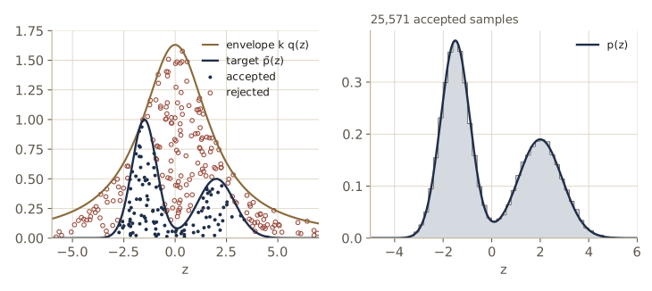
Rejection sampling uses a proposal distribution \(q(z)\) that we can sample from, and a constant \(k\) large enough that the envelope \(k q(z)\) lies above \(\tilde{p}(z)\) everywhere. Each step:
- Draw \(z_0 \sim q(z)\).
- Draw \(u_0\) uniformly on \([0, k q(z_0)]\).
- Accept \(z_0\) if \(u_0 \le \tilde{p}(z_0)\); otherwise discard it.
The pair \((z_0, u_0)\) is a uniformly distributed point under the curve \(k q(z)\). Keeping only the points under \(\tilde{p}(z)\) leaves points uniform under \(\tilde{p}\), and the horizontal coordinate of a uniform point under a curve is distributed in proportion to the curve’s height. In formulas: the density of drawing \(z\) and then accepting it is \(q(z) \cdot \tilde{p}(z)/(k q(z)) = \tilde{p}(z)/k\). Integrating over \(z\) gives the acceptance probability
\[p(\text{accept}) = \int \frac{\tilde{p}(z)}{k}\, dz = \frac{Z_p}{k},\]and dividing the first expression by the second gives the density of an accepted sample: \(\tilde{p}(z)/Z_p = p(z)\). So accepted samples are exact draws from \(p\), and the efficiency is the ratio of the area under \(\tilde{p}\) to the area under the envelope. We want \(k\) as small as possible while keeping the envelope above \(\tilde{p}\): \(k = \max_z \tilde{p}(z)/q(z)\).
Our target is a two-bump density, an unnormalized mixture of two Gaussian shapes. Since we built it ourselves we know its normalizer and its exact CDF, which we use only to check. The proposal is a Cauchy with scale 2, sampled by the transformation method. Its heavy tails make sure the ratio \(\tilde{p}/q\) is bounded; a Gaussian proposal narrower than the target in the tails would fail that test.
SQRT2PI = np.sqrt(2 * np.pi)

def p_tilde(z):
    """Unnormalized two-bump target."""
    return np.exp(-(z + 1.5)**2 / (2 * 0.6**2)) + 0.5 * np.exp(-(z - 2.0)**2 / (2 * 0.9**2))

def log_p_tilde(z):
    return np.log(p_tilde(z))

Z_p = SQRT2PI * (0.6 + 0.5 * 0.9)                  # exact normalizer (for checking)
w_mix = np.array([0.6, 0.5 * 0.9]) / (0.6 + 0.5 * 0.9)

def p_cdf(z):
    """Exact CDF of the normalized target (for checking only)."""
    return w_mix[0] * stats.norm.cdf(z, -1.5, 0.6) + w_mix[1] * stats.norm.cdf(z, 2.0, 0.9)

true_m2 = w_mix[0] * (1.5**2 + 0.6**2) + w_mix[1] * (2.0**2 + 0.9**2)   # exact E[z^2]; E[z] = 0

c_q, s_q = 0.0, 2.0
def q_pdf(z):
    return 1.0 / (np.pi * s_q * (1 + ((z - c_q) / s_q)**2))

grid = np.linspace(-30, 30, 600_001)
k = np.max(p_tilde(grid) / q_pdf(grid))            # smallest k with k q >= p_tilde on the grid
print(f"Z_p = {Z_p:.4f},  k = {k:.4f},  predicted acceptance Z_p / k = {Z_p / k:.4f}")
Z_p = 2.6320, k = 10.2464, predicted acceptance Z_p / k = 0.2569
def rejection_sample(p_tilde, q_pdf, q_sample, k, n, rng):
    """n proposals; returns the accepted samples and the acceptance rate."""
    z0 = q_sample(n, rng)
    u0 = rng.random(n) * k * q_pdf(z0)               # uniform on [0, k q(z0)]
    accept = u0 <= p_tilde(z0)
    return z0[accept], accept.mean()

rng_rej = np.random.default_rng(1112)
zs, rate = rejection_sample(p_tilde, q_pdf, lambda n, r: sample_cauchy(n, r, c_q, s_q),
                            k, 100_000, rng_rej)
print(f"accepted {len(zs)} of 100000: rate {rate:.4f}")
print(f"mean {zs.mean():.4f} (exact 0), E[z^2] {np.mean(zs**2):.4f} (exact {true_m2:.4f})")
print(f"KS p-value against the exact CDF: {stats.kstest(zs, p_cdf).pvalue:.3f}")
accepted 25571 of 100000: rate 0.2557
mean 0.0200 (exact 0), E[z^2] 3.5956 (exact 3.5529)
KS p-value against the exact CDF: 0.326
The acceptance rate matches the prediction \(Z_p/k\), and the accepted samples pass the test against the exact distribution.
Rejection sampling in many dimensions. The efficiency is an area ratio, and in high dimensions area ratios collapse. Take a target \(\mathcal{N}(\mathbf{0}, \sigma_p^2 \mathbf{I})\) in \(D\) dimensions and a slightly wider proposal \(\mathcal{N}(\mathbf{0}, \sigma_q^2 \mathbf{I})\). Both are normalized, the ratio \(p/q\) is largest at the origin, and there it equals the ratio of normalizing constants, \(k = (\sigma_q/\sigma_p)^D\). The acceptance rate \(1/k\) falls exponentially with \(D\).
ratio, n = 1.2, 200_000                            # sigma_q / sigma_p, number of proposals
for D in [1, 5, 10, 20]:
    z = ratio * rng.standard_normal((n, D))         # proposals, sigma_p = 1
    log_k = D * np.log(ratio)
    log_p_over_q = -0.5 * np.sum(z**2, axis=1) * (1 - 1 / ratio**2) + D * np.log(ratio)
    acc = np.mean(np.log(rng.random(n)) < log_p_over_q - log_k)
    print(f"D = {D:2d}: acceptance {acc:.4f}    1/k = {ratio**-D:.4f}")
print(f"sigma_q = 1.01 sigma_p in D = 1000: k = {1.01**1000:.0f}")
D =  1: acceptance 0.8335    1/k = 0.8333
D =  5: acceptance 0.4037    1/k = 0.4019
D = 10: acceptance 0.1639    1/k = 0.1615
D = 20: acceptance 0.0259    1/k = 0.0261
sigma_q = 1.01 sigma_p in D = 1000: k = 20959
Even a proposal only 1% wider than the target accepts about one sample in 21,000 in a thousand dimensions. Rejection sampling is a one- or two-dimensional tool, though it is often used inside larger algorithms to draw a single scalar.
Adaptive rejection sampling
Finding a tight envelope by hand is often the hard part. When the target is log-concave, meaning \(\ln p(z)\) is a concave function (its slope never increases), an envelope can be built automatically. Every tangent line of a concave function lies above it, so if we evaluate \(\ln p\) and its derivative at a few points \(z_1 < z_2 < \dots\), the minimum of the tangent lines is a piecewise-linear upper bound on \(\ln p\). Exponentiating gives an envelope made of exponential pieces, \(q(z) \propto k_i\, e^{-\lambda_i (z - z_{i-1})}\) on each interval, and each piece can be sampled by the inverse-CDF method for the exponential. After a rejection, the rejected point is added to the list of tangent points, so the envelope tightens exactly where it was loose. This is adaptive rejection sampling (Gilks and Wild); Bishop §11.1.3 describes it and variants that avoid derivatives or handle targets that are not log-concave. Many conditional distributions in Gibbs samplers for directed models are log-concave, which is where this method earns its keep.
Importance sampling
Often we do not need samples from \(p\) at all: we need an expectation. Importance sampling estimates it directly, using samples from a proposal \(q(\mathbf{z})\) that we can draw from. The idea is one line of algebra:
\[\mathbb{E}_p[f] = \int f(\mathbf{z}) \frac{p(\mathbf{z})}{q(\mathbf{z})}\, q(\mathbf{z})\, d\mathbf{z} \approx \frac{1}{L} \sum_{l=1}^{L} r_l\, f(\mathbf{z}^{(l)}), \qquad r_l = \frac{p(\mathbf{z}^{(l)})}{q(\mathbf{z}^{(l)})}, \quad \mathbf{z}^{(l)} \sim q.\]The importance weights \(r_l\) correct for sampling from the wrong distribution: points that \(q\) over-produces get small weights and points it under-produces get large ones. Every sample is used; none is rejected.
When only the unnormalized \(\tilde{p}\) (and perhaps an unnormalized \(\tilde{q}\)) is available, we write \(\tilde{r}_l = \tilde{p}(\mathbf{z}^{(l)}) / \tilde{q}(\mathbf{z}^{(l)})\). The same samples estimate the ratio of normalizers,
\[\frac{Z_p}{Z_q} = \frac{1}{Z_q} \int \tilde{p}(\mathbf{z})\, d\mathbf{z} = \int \frac{\tilde{p}(\mathbf{z})}{\tilde{q}(\mathbf{z})}\, q(\mathbf{z})\, d\mathbf{z} \approx \frac{1}{L} \sum_{l=1}^{L} \tilde{r}_l,\]and dividing one estimate by the other gives the self-normalized importance sampling estimate
\[\mathbb{E}_p[f] \approx \sum_{l=1}^{L} w_l\, f(\mathbf{z}^{(l)}), \qquad w_l = \frac{\tilde{r}_l}{\sum_{m} \tilde{r}_m}.\]It is slightly biased for finite \(L\) (it is a ratio of two estimates) but consistent. The normalized weights \(w_l\) also give a quick diagnostic, the importance-sampling effective sample size \(1/\sum_l w_l^2\). It equals \(L\) when all weights are equal and 1 when a single weight dominates.
Result. With samples \(\mathbf{z}^{(l)} \sim q\) and \(\tilde{r}_l = \tilde{p}(\mathbf{z}^{(l)})/\tilde{q}(\mathbf{z}^{(l)})\): \(\mathbb{E}_p[f] \approx \sum_l w_l f(\mathbf{z}^{(l)})\) with \(w_l = \tilde{r}_l / \sum_m \tilde{r}_m\), and \(Z_p/Z_q \approx \frac{1}{L}\sum_l \tilde{r}_l\). Compute the weights in log space and normalize with log-sum-exp.
We estimate \(\mathbb{E}[z]\), \(\mathbb{E}[z^2]\), and \(Z_p\) for the two-bump target with two Gaussian proposals: a wide one that covers both bumps, and a narrow one sitting on the left bump.
def importance(log_p_tilde, log_q, z):
    """Self-normalized importance sampling. Returns normalized weights w and log r~."""
    log_r = log_p_tilde(z) - log_q(z)
    return np.exp(log_r - logsumexp(log_r)), log_r

def log_normal(z, m, s):
    return -0.5 * ((z - m) / s)**2 - np.log(s * SQRT2PI)

L = 5000
rng_is = np.random.default_rng(1114)
for name, m, s in [("wide  N(0, 3^2)     ", 0.0, 3.0), ("narrow N(-1.5, 0.4^2)", -1.5, 0.4)]:
    z = m + s * rng_is.standard_normal(L)
    w, log_r = importance(log_p_tilde, lambda z: log_normal(z, m, s), z)
    Z_hat = np.exp(logsumexp(log_r) - np.log(L))    # q is normalized, so this estimates Z_p
    print(f"{name}: E[z] {np.sum(w * z):7.4f}  E[z^2] {np.sum(w * z**2):.4f}  "
          f"Z_p {Z_hat:.4f}  ESS {1 / np.sum(w**2):6.0f}")
print(f"exact                : E[z]  0.0000  E[z^2] {true_m2:.4f}  Z_p {Z_p:.4f}")
wide  N(0, 3^2)     : E[z] -0.0666  E[z^2] 3.5131  Z_p 2.6827  ESS   2647
narrow N(-1.5, 0.4^2): E[z] -1.5117  E[z^2] 2.7068  Z_p 1.5678  ESS   1291
exact                : E[z]  0.0000  E[z^2] 3.5529  Z_p 2.6320
The wide proposal gets all three numbers roughly right. The narrow one is badly wrong: it reports a mean near \(-1.5\) and misses about 40% of the normalizer, because it essentially never proposes a point near the right bump. And nothing in its own output warns us: an effective sample size of more than a thousand looks healthy. The trouble is the region it never sampled, and no statistic of the samples it did draw can reveal that.
Watch out. Importance sampling fails silently when \(q\) is small where \(p\) (or \(p f\)) is large. The weights of the samples you did draw can look perfectly well behaved; the problem is the region you never sampled. A proposal should have heavier tails than the target, never lighter, and in high dimensions a good match is hard to find, for the same reason rejection sampling fails there.
Importance sampling in graphical models. Return to the sprinkler network and the evidence \(W = 1\). One crude option, uniform sampling, sets the observed variables to their values and draws every other variable uniformly; the weight of a sample is then proportional to its joint probability \(p(\mathbf{z})\). It works poorly when the posterior is far from uniform. A better option is likelihood weighting: sample the unobserved nodes by ancestral sampling, clamp each observed node to its value, and weight the sample by the product of the conditional probabilities of the observed nodes given their sampled parents, \(r(\mathbf{z}) = \prod_{i \in \text{evidence}} p(z_i \mid \mathrm{pa}_i)\). The proposal differs from the posterior only in the factors for the observed nodes, so those factors are exactly the importance weights.
c, s, r, _ = ancestral(n_bn, rng)                  # ancestral sample; W is ignored and clamped to 1
weights = p_wet(s, r)                              # r(z) = p(W = 1 | S, R)
print(f"likelihood weighting: p(R=1 | W=1) ~ {np.sum(weights * r) / weights.sum():.4f}  "
      f"(exact {exact:.4f}),  ESS {weights.sum()**2 / np.sum(weights**2):.0f} of {n_bn}")
likelihood weighting: p(R=1 | W=1) ~ 0.4894 (exact 0.4909), ESS 13853 of 20000
Nothing was thrown away, and the estimate is close to the exact value. Weighting schemes that keep adapting the proposal toward the current posterior estimate also exist (Bishop §11.1.4 mentions self-importance sampling).
Sampling-importance-resampling
Rejection sampling needs the constant \(k\), which can be hard to find. Sampling-importance-resampling (SIR) produces approximate samples from \(p\) without it. Draw \(L\) samples from \(q\), compute the normalized weights \(w_l\) as above, then draw \(L\) new samples, with replacement, from the discrete distribution that puts probability \(w_l\) on \(\mathbf{z}^{(l)}\).
Why does this work? For a scalar \(z\), the probability that a resampled value is at most \(a\) is
\[\sum_{l:\, z^{(l)} \le a} w_l = \frac{\frac{1}{L}\sum_l I(z^{(l)} \le a)\, \tilde{p}(z^{(l)})/q(z^{(l)})}{\frac{1}{L}\sum_l \tilde{p}(z^{(l)})/q(z^{(l)})} \;\longrightarrow\; \frac{\int I(z \le a)\, \tilde{p}(z)\, dz}{\int \tilde{p}(z)\, dz} \quad (L \to \infty),\]where \(I(\cdot)\) is 1 when its argument is true and 0 otherwise. The limit is the CDF of \(p\), so the resampled values are distributed according to \(p\) in the limit, and again \(Z_p\) was never needed. For finite \(L\) the result is approximate, and it is exact when \(q = p\) (all weights equal \(1/L\)). If you only need moments, use the weighted sums directly: resampling adds noise without adding information.
z = 3.0 * rng_is.standard_normal(20_000)
w, _ = importance(log_p_tilde, lambda z: log_normal(z, 0.0, 3.0), z)
z_sir = rng_is.choice(z, size=20_000, replace=True, p=w)
print(f"SIR: mean {z_sir.mean():.4f}, E[z^2] {np.mean(z_sir**2):.4f} (exact 0, {true_m2:.4f}), "
      f"{len(np.unique(z_sir))} distinct values")
print(f"KS p-value against the exact CDF: {stats.kstest(z_sir, p_cdf).pvalue:.3f}")
SIR: mean -0.0219, E[z^2] 3.5378 (exact 0, 3.5529), 9750 distinct values
KS p-value against the exact CDF: 0.111
About half of the resampled values are repeats, which is the price of resampling. SIR is the core step of particle filters, which track a changing posterior through time (module 13).
Sampling and the EM algorithm
Sampling also helps with maximum likelihood. The E step of EM (module 09) needs the expected complete-data log likelihood
\[Q(\boldsymbol{\theta}, \boldsymbol{\theta}^{\text{old}}) = \int p(\mathbf{Z} \mid \mathbf{X}, \boldsymbol{\theta}^{\text{old}}) \ln p(\mathbf{Z}, \mathbf{X} \mid \boldsymbol{\theta})\, d\mathbf{Z},\]and for some models this integral has no closed form. If we can sample from the posterior over the latent variables, we can replace it by an average over samples \(\mathbf{Z}^{(l)} \sim p(\mathbf{Z} \mid \mathbf{X}, \boldsymbol{\theta}^{\text{old}})\):
\[Q(\boldsymbol{\theta}, \boldsymbol{\theta}^{\text{old}}) \approx \frac{1}{L} \sum_{l=1}^{L} \ln p(\mathbf{Z}^{(l)}, \mathbf{X} \mid \boldsymbol{\theta}),\]and maximize that in the M step as usual. This is the Monte Carlo EM algorithm. Adding \(\ln p(\boldsymbol{\theta})\) to \(Q\) turns it into a search for the MAP estimate. With a single sample per E step (\(L = 1\)) in a mixture model, each data point is assigned to one component at random according to its responsibilities; this is stochastic EM.
Here is a mixture of two unit-variance Gaussians with equal weights and unknown means, where the exact E step is available for comparison. Sampling the component labels replaces the responsibilities by label frequencies.
rng_em = np.random.default_rng(1116)
x = np.concatenate([rng_em.normal(-1.0, 1.0, 120), rng_em.normal(2.0, 1.0, 80)])

def responsibilities(x, mu):
    """gamma_nk for a two-component, unit-variance, equal-weight Gaussian mixture."""
    log_g = -0.5 * (x[:, None] - mu[None, :])**2
    return np.exp(log_g - logsumexp(log_g, axis=1, keepdims=True))

def em_means(x, mu, iters, L=None, rng=None):
    """EM for the two means; with L given, the E step uses L sampled label sets."""
    trace = []
    for _ in range(iters):
        gam = responsibilities(x, mu)
        if L is not None:                           # Monte Carlo E step
            z1 = rng.random((L, len(x))) < gam[:, 1]
            gam = np.stack([(~z1).mean(axis=0), z1.mean(axis=0)], axis=1)
        mu = (gam * x[:, None]).sum(axis=0) / gam.sum(axis=0)     # M step
        trace.append(mu.copy())
    return np.array(trace)

mu_init = np.array([-0.5, 0.5])
for name, tr in [("exact EM     ", em_means(x, mu_init, 40)),
                 ("MC-EM, L=100 ", em_means(x, mu_init, 40, L=100, rng=rng_em)),
                 ("stochastic EM", em_means(x, mu_init, 40, L=1, rng=rng_em))]:
    print(name, " last three iterates:", "  ".join(f"({a:.3f}, {b:.3f})" for a, b in tr[-3:]))
exact EM       last three iterates: (-1.029, 2.030)  (-1.029, 2.030)  (-1.029, 2.030)
MC-EM, L=100   last three iterates: (-1.031, 2.024)  (-1.032, 2.024)  (-1.033, 2.027)
stochastic EM  last three iterates: (-1.068, 1.972)  (-1.051, 2.059)  (-1.058, 2.030)
Exact EM has converged; Monte Carlo EM with 100 samples jitters around the same answer in the third decimal; stochastic EM wanders more widely, since its iterates are themselves random and never converge to a point. In practice one increases \(L\) as the iterations proceed.
The fully Bayesian version treats \(\boldsymbol{\theta}\) as random too. The data augmentation or IP algorithm alternates two steps. The imputation (I) step draws \(\boldsymbol{\theta}^{(l)}\) from the current approximation to \(p(\boldsymbol{\theta} \mid \mathbf{X})\) and then \(\mathbf{Z}^{(l)} \sim p(\mathbf{Z} \mid \boldsymbol{\theta}^{(l)}, \mathbf{X})\), for \(l = 1, \dots, L\). The posterior (P) step updates the approximation to \(\frac{1}{L}\sum_l p(\boldsymbol{\theta} \mid \mathbf{Z}^{(l)}, \mathbf{X})\), a mixture we can sample from if the complete-data posterior is tractable. Alternating draws of the latent variables and the parameters is exactly the pattern of the Gibbs sampler below, where we stop distinguishing parameters from latent variables.
Markov chain Monte Carlo
Rejection and importance sampling draw every sample from the same fixed proposal, and in high dimensions no fixed proposal is good enough. Markov chain Monte Carlo (MCMC) lets the proposal depend on where we are. It keeps a current state \(\mathbf{z}^{(\tau)}\), proposes a nearby candidate from \(q(\mathbf{z} \mid \mathbf{z}^{(\tau)})\), and accepts or rejects it by a rule that makes the sequence of states converge to the target distribution. As before, only \(\tilde{p}(\mathbf{z})\) is needed.
The Metropolis algorithm and random walks
The first such rule is the Metropolis algorithm (Metropolis and coauthors, 1953). The proposal must be symmetric, \(q(\mathbf{z}_A \mid \mathbf{z}_B) = q(\mathbf{z}_B \mid \mathbf{z}_A)\), for example a Gaussian centered at the current state. A candidate \(\mathbf{z}^\star\) is accepted with probability
\[A(\mathbf{z}^\star, \mathbf{z}^{(\tau)}) = \min\left(1, \frac{\tilde{p}(\mathbf{z}^\star)}{\tilde{p}(\mathbf{z}^{(\tau)})}\right).\]In code: draw \(u\) uniform on \((0, 1)\) and accept if \(u < A\). Uphill moves are always accepted, downhill moves sometimes. If the candidate is accepted, \(\mathbf{z}^{(\tau+1)} = \mathbf{z}^\star\); if not, \(\mathbf{z}^{(\tau+1)} = \mathbf{z}^{(\tau)}\), and the current state is recorded again. This repetition is essential and different from rejection sampling, where rejected draws simply vanish. Successive states are correlated, so the effective sample size is smaller than the number of steps.
Before proving that this works, look at what makes it slow. A chain on the integers that stays put with probability \(\tfrac{1}{2}\) and moves one step left or right with probability \(\tfrac{1}{4}\) each is a random walk. Starting from 0, each step adds an independent increment with mean 0 and variance \(\tfrac{1}{2}\), so after \(\tau\) steps \(\mathbb{E}[z^{(\tau)}] = 0\) and \(\mathbb{E}[(z^{(\tau)})^2] = \tau/2\).
walks = np.cumsum(rng.choice([-1, 0, 0, 1], size=(4000, 400)), axis=1)   # 4000 walks, 400 steps
for tau in [25, 100, 400]:
    zt = walks[:, tau - 1]
    print(f"after {tau:3d} steps: mean {zt.mean():6.3f}   E[z^2] {np.mean(zt**2):6.1f}   (tau/2 = {tau / 2:.1f})")
after  25 steps: mean -0.064   E[z^2]   12.4   (tau/2 = 12.5)
after 100 steps: mean  0.016   E[z^2]   48.3   (tau/2 = 50.0)
after 400 steps: mean  0.174   E[z^2]  199.7   (tau/2 = 200.0)
The typical distance traveled grows like \(\sqrt{\tau}\): to go ten times farther, a random walk needs a hundred times as many steps. MCMC methods that explore by small random steps inherit this behavior, and much of the design of better samplers is about avoiding it.
Markov chains
A first-order Markov chain is a sequence of random variables \(\mathbf{z}^{(1)}, \mathbf{z}^{(2)}, \dots\) in which each depends on the past only through its predecessor:
\[p(\mathbf{z}^{(m+1)} \mid \mathbf{z}^{(1)}, \dots, \mathbf{z}^{(m)}) = p(\mathbf{z}^{(m+1)} \mid \mathbf{z}^{(m)}).\]As a graphical model it is a chain of nodes. It is specified by an initial distribution and transition probabilities \(T_m(\mathbf{z}^{(m)}, \mathbf{z}^{(m+1)}) = p(\mathbf{z}^{(m+1)} \mid \mathbf{z}^{(m)})\); it is homogeneous if these are the same at every step, and then we write \(T(\mathbf{z}, \mathbf{z}')\). The marginal distribution evolves by
\[p(\mathbf{z}^{(m+1)}) = \sum_{\mathbf{z}^{(m)}} T(\mathbf{z}^{(m)}, \mathbf{z}^{(m+1)})\, p(\mathbf{z}^{(m)}).\]For a chain on \(K\) states, \(T\) is a \(K \times K\) matrix with rows summing to 1 (row = current state, column = next state), and if \(\mathbf{p}^{(m)}\) is the row vector of marginal probabilities, then \(\mathbf{p}^{(m+1)} = \mathbf{p}^{(m)} \mathbf{T}\).
Definition. A distribution \(p^\star\) is invariant (or stationary) for the chain if one step leaves it unchanged: \(p^\star(\mathbf{z}) = \sum_{\mathbf{z}'} T(\mathbf{z}', \mathbf{z})\, p^\star(\mathbf{z}')\), or \(\mathbf{p}^\star = \mathbf{p}^\star \mathbf{T}\) for a finite chain. The chain is ergodic if \(p(\mathbf{z}^{(m)}) \to p^\star\) as \(m \to \infty\) from every initial distribution; \(p^\star\) is then called the equilibrium distribution, and it is unique.
A chain can have many invariant distributions (if \(T\) is the identity, every distribution is invariant), and an invariant distribution need not be reached (a chain can oscillate forever). MCMC needs both properties: the target must be invariant, and the chain must be ergodic so that it forgets its starting point. Ergodicity holds under mild conditions on the chain and the target (Bishop cites Neal, 1993); roughly, every region of positive probability must be reachable and the chain must not cycle deterministically.
For a finite chain, \(\mathbf{p}^\star = \mathbf{p}^\star \mathbf{T}\) says \(\mathbf{p}^\star\) is a left eigenvector of \(\mathbf{T}\) with eigenvalue 1, that is, an ordinary eigenvector of \(\mathbf{T}^{\mathrm{T}}\). Here is a four-state chain. We find its stationary distribution three ways: as an eigenvector, by propagating two different initial distributions for 50 steps, and by simulating the chain and counting visits.
T = np.array([[0.5, 0.3, 0.2, 0.0],
              [0.1, 0.6, 0.2, 0.1],
              [0.0, 0.3, 0.4, 0.3],
              [0.2, 0.0, 0.3, 0.5]])               # T[i, j] = p(next = j | current = i)

evals, evecs = np.linalg.eig(T.T)                  # left eigenvectors of T
i1 = np.argmin(np.abs(evals - 1))
p_star = np.real(evecs[:, i1]) / np.real(evecs[:, i1]).sum()
print("eigenvalue moduli:", np.sort(np.abs(evals))[::-1])
print("stationary (eigenvector):  ", p_star)
for p0 in [np.array([1.0, 0, 0, 0]), np.array([0, 0, 0, 1.0])]:
    p = p0
    for m in range(50):
        p = p @ T                                  # p^(m+1) = p^(m) T
    print("p(z^(50)) from", p0, ":", p)

def simulate_chain(T, z0, n, rng):
    """One trajectory of length n of a finite Markov chain."""
    cum = np.cumsum(T, axis=1)
    u = rng.random(n)
    z = np.empty(n, dtype=int)
    z[0] = z0
    for t in range(1, n):
        z[t] = np.searchsorted(cum[z[t - 1]], u[t], side="right")
    return z

zc = simulate_chain(T, 0, 200_000, rng)
print("visit frequencies:         ", np.bincount(zc, minlength=4) / len(zc))
eigenvalue moduli: [1.     0.431  0.431  0.1453]
stationary (eigenvector):   [0.159  0.3286 0.2792 0.2332]
p(z^(50)) from [1. 0. 0. 0.] : [0.159  0.3286 0.2792 0.2332]
p(z^(50)) from [0. 0. 0. 1.] : [0.159  0.3286 0.2792 0.2332]
visit frequencies:          [0.1597 0.3285 0.2791 0.2327]
All three agree. The second-largest eigenvalue modulus, 0.431, controls how fast the chain forgets its start: the distance to equilibrium shrinks roughly like \(0.431^m\), which after 50 steps is far below printing precision.
Detailed balance. A convenient sufficient condition for \(p^\star\) to be invariant is detailed balance:
\[p^\star(\mathbf{z})\, T(\mathbf{z}, \mathbf{z}') = p^\star(\mathbf{z}')\, T(\mathbf{z}', \mathbf{z}) \quad \text{for all } \mathbf{z}, \mathbf{z}'.\]It says that in equilibrium the probability flow from \(\mathbf{z}\) to \(\mathbf{z}'\) equals the flow back. Summing both sides over \(\mathbf{z}'\) shows that it implies invariance:
\[\sum_{\mathbf{z}'} p^\star(\mathbf{z}')\, T(\mathbf{z}', \mathbf{z}) = \sum_{\mathbf{z}'} p^\star(\mathbf{z})\, T(\mathbf{z}, \mathbf{z}') = p^\star(\mathbf{z}) \sum_{\mathbf{z}'} T(\mathbf{z}, \mathbf{z}') = p^\star(\mathbf{z}).\]A chain satisfying detailed balance is called reversible: run in equilibrium, it looks statistically the same forwards and backwards. The condition is sufficient, not necessary. The chain above has an invariant distribution but is not reversible, and neither is the two-state chain that always switches state: its invariant distribution is \((\tfrac{1}{2}, \tfrac{1}{2})\), but started in state 0 it alternates forever and never converges, so it is not ergodic.
To design a chain for a given target \(\mathbf{p}^\star\), detailed balance is the easy thing to aim for. Here we build a Metropolis chain on four states: propose one of the other three states uniformly and accept with probability \(\min(1, p^\star_j / p^\star_i)\). We check detailed balance for both chains, and invariance for the new one.
F = p_star[:, None] * T                            # F[i, j] = p*_i T_ij, the flow from i to j
print(f"first chain:      max |p*_i T_ij - p*_j T_ji| = {np.max(np.abs(F - F.T)):.4f}")

target = np.array([0.1, 0.2, 0.3, 0.4])
K = len(target)
T_mh = np.zeros((K, K))
for i in range(K):
    for j in range(K):
        if j != i:
            T_mh[i, j] = (1 / (K - 1)) * min(1.0, target[j] / target[i])   # propose, then accept
    T_mh[i, i] = 1 - T_mh[i].sum()                 # rejected proposals stay put
F = target[:, None] * T_mh
print(f"Metropolis chain: max |p*_i T_ij - p*_j T_ji| = {np.max(np.abs(F - F.T)):.1e}")
print("target @ T_mh =", target @ T_mh)
first chain:      max |p*_i T_ij - p*_j T_ji| = 0.0466
Metropolis chain: max |p*_i T_ij - p*_j T_ji| = 1.4e-17
target @ T_mh = [0.1 0.2 0.3 0.4]
In practice, transitions are often assembled from simpler base transitions \(B_1, \dots, B_K\), each of which leaves \(p^\star\) invariant. We can pick one at random each step, \(T = \sum_k \alpha_k B_k\) with mixing weights \(\alpha_k \ge 0\) summing to 1, or apply them one after another. Either way \(p^\star\) stays invariant. A random mixture of reversible transitions is reversible; a fixed sequence \(B_1 B_2 \cdots B_K\) generally is not, but the symmetric sequence \(B_1, \dots, B_K, B_K, \dots, B_1\) is. A common case is base transitions that each change only some of the variables, which is exactly what Gibbs sampling does.
The Metropolis–Hastings algorithm
Metropolis–Hastings (Hastings, 1970) allows asymmetric proposals. From state \(\mathbf{z}\), draw \(\mathbf{z}^\star \sim q_k(\mathbf{z}^\star \mid \mathbf{z})\) and accept with probability
\[A_k(\mathbf{z}^\star, \mathbf{z}) = \min\left(1, \frac{\tilde{p}(\mathbf{z}^\star)\, q_k(\mathbf{z} \mid \mathbf{z}^\star)}{\tilde{p}(\mathbf{z})\, q_k(\mathbf{z}^\star \mid \mathbf{z})}\right),\]where \(k\) indexes a family of proposal types that may be mixed or alternated. The constant \(Z_p\) cancels in the ratio, and for a symmetric proposal the \(q\) factors cancel, giving back the Metropolis rule.
To prove that \(p\) is invariant we check detailed balance. For \(\mathbf{z}' \ne \mathbf{z}\), the transition density is “propose, then accept”: \(T(\mathbf{z}, \mathbf{z}') = q_k(\mathbf{z}' \mid \mathbf{z})\, A_k(\mathbf{z}', \mathbf{z})\). Multiply by \(p(\mathbf{z})\) and bring \(p(\mathbf{z}) q_k(\mathbf{z}' \mid \mathbf{z})\) inside the minimum:
\[\begin{aligned} p(\mathbf{z})\, q_k(\mathbf{z}' \mid \mathbf{z})\, A_k(\mathbf{z}', \mathbf{z}) &= \min\big(p(\mathbf{z})\, q_k(\mathbf{z}' \mid \mathbf{z}),\; p(\mathbf{z}')\, q_k(\mathbf{z} \mid \mathbf{z}')\big) \\ &= p(\mathbf{z}')\, q_k(\mathbf{z} \mid \mathbf{z}')\, A_k(\mathbf{z}, \mathbf{z}'). \end{aligned}\]The middle expression is symmetric in \(\mathbf{z}\) and \(\mathbf{z}'\), so the flow from \(\mathbf{z}\) to \(\mathbf{z}'\) equals the flow back. (Transitions from a state to itself trivially satisfy detailed balance.) Together with ergodicity, which holds for instance whenever \(q_k(\mathbf{z}' \mid \mathbf{z}) > 0\) for all pairs and the target is positive everywhere, the distribution of \(\mathbf{z}^{(\tau)}\) converges to \(p\).
Here is random-walk Metropolis with an isotropic Gaussian proposal of standard deviation step. It runs \(C\) independent chains at once (one per row of z) so that NumPy works on arrays rather than single numbers; each chain is an ordinary Metropolis chain.
Lam_c = np.linalg.solve(Sigma_c, np.eye(2))       # precision matrix of the test Gaussian

def log_p_gauss(z):
    """ln p~(z) = -z^T Lambda z / 2 for each row of z."""
    return -0.5 * np.sum((z @ Lam_c) * z, axis=1)

def metropolis(log_p, z0, step, n_steps, rng):
    """Random-walk Metropolis on C chains at once. z0: (C, D).
    Returns the states, shape (n_steps, C, D), and the acceptance rate."""
    z = np.array(z0, float)
    lp = log_p(z)
    C, D = z.shape
    out = np.empty((n_steps, C, D))
    n_acc = 0
    for t in range(n_steps):
        z_star = z + step * rng.standard_normal((C, D))     # symmetric proposal
        lp_star = log_p(z_star)
        accept = np.log(rng.random(C)) < lp_star - lp       # u < p~(z*) / p~(z)
        z[accept], lp[accept] = z_star[accept], lp_star[accept]
        out[t] = z                                          # a rejection repeats the state
        n_acc += accept.sum()
    return out, n_acc / (n_steps * C)

rng_path = np.random.default_rng(1121)
for step in [0.2, 1.6]:
    path, acc = metropolis(log_p_gauss, np.array([[-1.5, -1.5]]), step, 200, rng_path)
    print(f"step {step}: {round(acc * 200)} of 200 proposals accepted; final state {path[-1, 0]}")
step 0.2: 115 of 200 proposals accepted; final state [-0.5452 -0.5606]
step 1.6: 18 of 200 proposals accepted; final state [-1.1795 -1.2049]
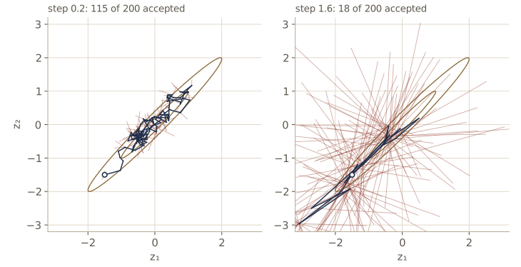
Step size and the cost of a random walk
The proposal width sets a trade-off. Small steps are nearly always accepted but move little, so the chain performs a slow random walk. Large steps mostly land off the thin ridge of high probability and are rejected, so the chain sits still. To see the effect on accuracy, we run 20 chains of 5000 steps for each step size, starting them from exact samples (so no warm-up is needed), and measure the integrated autocorrelation time of the coordinate along the long axis of the ellipse, averaged over the chains.
def major_axis(samples):
    """Coordinate along the long axis (1, 1)/sqrt(2) of the test Gaussian."""
    return (samples[..., 0] + samples[..., 1]) / np.sqrt(2)

def mean_iat(x):
    """Average integrated autocorrelation time over chains; x has shape (n_steps, C)."""
    return np.mean([iat(x[:, c]) for c in range(x.shape[1])])

rng_mh = np.random.default_rng(1122)
z0 = sample_gaussian(np.zeros(2), L_c, 20, rng_mh)          # 20 chains, started in equilibrium
print(" step   accept   IAT (long axis)   ESS per 1000 steps")
for step in [0.05, 0.1, 0.2, 0.4, 0.8, 1.6, 3.2]:
    s, acc = metropolis(log_p_gauss, z0, step, 5000, rng_mh)
    tau = mean_iat(major_axis(s))
    print(f"{step:5.2f}   {acc:.3f}     {tau:7.1f}            {1000 / tau:5.1f}")
 step   accept   IAT (long axis)   ESS per 1000 steps
 0.05   0.888       799.5              1.3
 0.10   0.780       553.3              1.8
 0.20   0.604       255.0              3.9
 0.40   0.378       135.4              7.4
 0.80   0.197        76.8             13.0
 1.60   0.088        62.1             16.1
 3.20   0.031        73.1             13.7
With steps near \(\sigma_{\min} \approx 0.14\), most proposals are accepted and it takes several hundred steps to produce one effectively independent sample. The best setting here accepts under 10% of proposals, and even then the chain needs about 60 steps per effective sample.
The argument for the cost goes like this. To keep the acceptance rate reasonable in a general problem, the step size \(s\) must be comparable to the smallest length scale \(\sigma_{\min}\); steps much larger than that almost always leave the ridge. Along the long direction the chain then does a random walk with steps of size about \(\sigma_{\min}\), and by the \(\sqrt{\tau}\) law it needs about \((\sigma_{\max}/\sigma_{\min})^2\) steps to cross a distance \(\sigma_{\max}\). We can test the scaling by stretching the ellipse while keeping \(s = 1.5\, \sigma_{\min}\):
rng_sc = np.random.default_rng(1123)
R45 = np.array([[1.0, -1.0], [1.0, 1.0]]) / np.sqrt(2)      # rotate the axes by 45 degrees
print(" sigma_max/sigma_min   accept      IAT    IAT / ratio^2")
for ratio in [2.5, 5, 10, 20]:
    s_min = 1.0 / ratio                                       # sigma_max = 1
    Sig = R45 @ np.diag([1.0, s_min**2]) @ R45.T
    Lam = np.linalg.solve(Sig, np.eye(2))
    lp = lambda z: -0.5 * np.sum((z @ Lam) * z, axis=1)
    z0 = sample_gaussian(np.zeros(2), np.linalg.cholesky(Sig), 40, rng_sc)
    s, acc = metropolis(lp, z0, 1.5 * s_min, 20_000, rng_sc)
    tau = mean_iat(major_axis(s))
    print(f"{ratio:12.1f}          {acc:.3f}   {tau:7.1f}      {tau / ratio**2:.2f}")
 sigma_max/sigma_min   accept      IAT    IAT / ratio^2
         2.5          0.528      25.6      4.09
         5.0          0.569      86.3      3.45
        10.0          0.583     339.8      3.40
        20.0          0.588    1178.4      2.95
As the ellipse gets eight times more elongated, the autocorrelation time grows by a factor of more than 40, while \(\tau / (\sigma_{\max}/\sigma_{\min})^2\) stays between about 3 and 4: the cost is quadratic in the ratio of length scales, as the random-walk argument predicts. (The estimates for the longest ellipse are the noisiest, because 20,000 steps is fewer than twenty autocorrelation times.)
Note. In two dimensions, the step-size table showed that a step much larger than \(\sigma_{\min}\) can do better than the random-walk argument suggests: many proposals are rejected, but the accepted ones travel far. Bishop §11.2.2 notes this and a sharper result of Neal: for a Gaussian in many dimensions the cost scales with the square of the ratio of the largest to the second-smallest standard deviation. The practical lesson does not change: when length scales differ widely across directions, random-walk Metropolis mixes slowly, and a rescaling of the variables (if one is known) or a sampler that uses more information about \(p\) is needed.
In practice. Real MCMC runs start somewhere arbitrary, not in equilibrium, so the first part of the chain (the burn-in or warm-up) is discarded. Run several chains from dispersed starting points and compare them; report effective sample sizes, not raw chain lengths. Thinning (keeping every \(M\)th state) makes the kept states closer to independent but never increases the information in the chain; it only saves storage.
Gibbs sampling
Gibbs sampling, introduced by Geman and Geman (1984), is the simplest MCMC method to describe, and one of the most used. Its transitions change one variable at a time, drawing it from its full conditional distribution given all the others. For \(\mathbf{z} = (z_1, \dots, z_M)\), one sweep is:
- Draw \(z_1^{(\tau+1)} \sim p(z_1 \mid z_2^{(\tau)}, z_3^{(\tau)}, \dots, z_M^{(\tau)})\).
- Draw \(z_2^{(\tau+1)} \sim p(z_2 \mid z_1^{(\tau+1)}, z_3^{(\tau)}, \dots, z_M^{(\tau)})\).
- Continue through \(z_M^{(\tau+1)} \sim p(z_M \mid z_1^{(\tau+1)}, \dots, z_{M-1}^{(\tau+1)})\).
Each draw uses the newest values of the other variables. The variables can be visited in a fixed order (systematic scan) or chosen at random each step (random scan).
Why it works. Consider the update of \(z_i\), and write \(\mathbf{z}_{\setminus i}\) for all the other variables. Suppose the current state is distributed according to \(p(\mathbf{z}) = p(z_i \mid \mathbf{z}_{\setminus i})\, p(\mathbf{z}_{\setminus i})\). The update leaves \(\mathbf{z}_{\setminus i}\) alone, so it still has marginal \(p(\mathbf{z}_{\setminus i})\), and it draws \(z_i\) afresh from the correct conditional. The new state therefore has the joint distribution \(p(z_i \mid \mathbf{z}_{\setminus i})\, p(\mathbf{z}_{\setminus i}) = p(\mathbf{z})\): each update leaves \(p\) invariant, and so does a sweep.
Gibbs sampling is a special case of Metropolis–Hastings. Take the update of \(z_k\) as a proposal \(q_k(\mathbf{z}^\star \mid \mathbf{z}) = p(z_k^\star \mid \mathbf{z}_{\setminus k})\) with \(\mathbf{z}^\star_{\setminus k} = \mathbf{z}_{\setminus k}\). Using \(p(\mathbf{z}) = p(z_k \mid \mathbf{z}_{\setminus k})\, p(\mathbf{z}_{\setminus k})\), the Metropolis–Hastings ratio is
\[\frac{p(\mathbf{z}^\star)\, q_k(\mathbf{z} \mid \mathbf{z}^\star)}{p(\mathbf{z})\, q_k(\mathbf{z}^\star \mid \mathbf{z})} = \frac{p(z_k^\star \mid \mathbf{z}_{\setminus k})\, p(\mathbf{z}_{\setminus k})\, p(z_k \mid \mathbf{z}_{\setminus k})}{p(z_k \mid \mathbf{z}_{\setminus k})\, p(\mathbf{z}_{\setminus k})\, p(z_k^\star \mid \mathbf{z}_{\setminus k})} = 1,\]so every proposal is accepted. There is no step size to tune.
Invariance is not the whole story; the chain must also be ergodic. A sufficient condition is that no full conditional is zero anywhere, since then any state can be reached from any other in one sweep. When some conditionals have zeros, ergodicity needs a separate argument, and it can fail (exercise 8). As with any MCMC method, successive states are correlated, and early states depend on the starting point.
Gibbs sampling a correlated Gaussian
For our test Gaussian with unit variances and correlation \(\rho\), the full conditionals come from the Gaussian conditioning formulas of module 02:
\[p(z_1 \mid z_2) = \mathcal{N}(z_1 \mid \rho z_2,\, 1 - \rho^2), \qquad p(z_2 \mid z_1) = \mathcal{N}(z_2 \mid \rho z_1,\, 1 - \rho^2).\]The conditional standard deviation \(\sqrt{1 - \rho^2} \approx 0.2\) is much smaller than the marginal standard deviation 1, so each move is short. We can predict the autocorrelation exactly. After one sweep, \(z_1^{(\tau+1)} = \rho z_2^{(\tau)} + \text{noise}\) and \(z_2^{(\tau)} = \rho z_1^{(\tau)} + \text{noise}\), so \(z_1^{(\tau+1)} = \rho^2 z_1^{(\tau)} + \text{noise}\): from sweep to sweep, \(z_1\) is an autoregressive sequence with coefficient \(\rho^2\), and its autocorrelation time is \((1 + \rho^2)/(1 - \rho^2)\).
The function below also has an over-relaxation parameter \(\alpha\), explained below; \(\alpha = 0\) is ordinary Gibbs sampling.
def gibbs_gauss2(rho, z0, n_sweeps, rng, alpha=0.0):
    """Systematic-scan Gibbs (alpha = 0) or over-relaxed Gibbs (-1 < alpha < 0) for a
    zero-mean bivariate Gaussian with unit variances and correlation rho; C chains at once."""
    z = np.array(z0, float)
    C = z.shape[0]
    s = np.sqrt(1 - rho**2)                         # conditional standard deviation
    out = np.empty((n_sweeps, C, 2))
    for t in range(n_sweeps):
        for i, j in [(0, 1), (1, 0)]:
            m = rho * z[:, j]                       # conditional mean of z_i given z_j
            z[:, i] = m + alpha * (z[:, i] - m) + s * np.sqrt(1 - alpha**2) * rng.standard_normal(C)
        out[t] = z
    return out

rng_g = np.random.default_rng(1131)
rho = 0.98
z0 = sample_gaussian(np.zeros(2), L_c, 20, rng_g)
s = gibbs_gauss2(rho, z0, 5000, rng_g)
print(f"Gibbs: IAT of z1 {mean_iat(s[..., 0]):.1f}  (theory (1 + rho^2)/(1 - rho^2) = {(1 + rho**2) / (1 - rho**2):.1f});"
      f"  IAT long axis {mean_iat(major_axis(s)):.1f}")
print(f"sample mean {s.reshape(-1, 2).mean(axis=0)},  sample corr {np.corrcoef(s.reshape(-1, 2).T)[0, 1]:.4f}")
Gibbs: IAT of z1 51.4  (theory (1 + rho^2)/(1 - rho^2) = 49.5);  IAT long axis 51.9
sample mean [-0.0472 -0.0471],  sample corr 0.9800
The measured autocorrelation time agrees with the prediction of about 50 sweeps. In terms of the book’s picture: the conditional width \(l = \sqrt{1-\rho^2}\) sets the step length, the marginal width \(L = 1\) is the distance to cover, and a random walk needs on the order of \((L/l)^2 = 1/(1-\rho^2) \approx 25\) sweeps, the same order as what we measured.
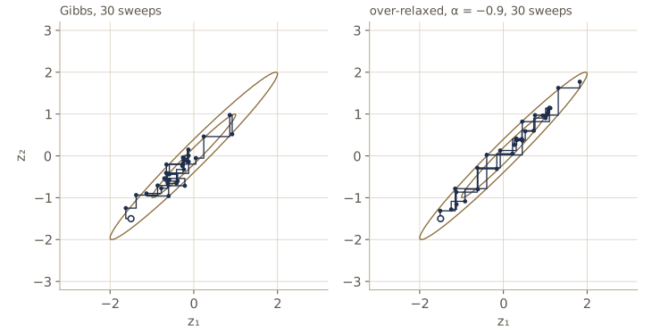
If we could rotate the coordinates to align with the ellipse, Gibbs sampling would produce independent samples at once. For this toy problem that is easy; for a real posterior we usually do not know such a transformation.
A Bayesian example: mean and precision of a Gaussian
Gibbs sampling shines when the full conditionals are standard distributions even though the joint posterior is not. Take \(N\) observations \(x_n \sim \mathcal{N}(\mu, \lambda^{-1})\) with unknown mean \(\mu\) and precision \(\lambda\), and independent priors \(\mu \sim \mathcal{N}(\mu_0, s_0)\) (mean \(\mu_0\), variance \(s_0\)) and \(\lambda \sim \operatorname{Gam}(a_0, b_0)\). Unlike the normal-gamma prior of module 02, this prior is not conjugate for the pair, and the joint posterior \(p(\mu, \lambda \mid \mathbf{x})\) has no standard form. But each full conditional does.
For \(\mu\), collect the terms in the exponent that depend on \(\mu\):
\[\ln p(\mu \mid \lambda, \mathbf{x}) = -\frac{(\mu - \mu_0)^2}{2 s_0} - \frac{\lambda}{2} \sum_{n=1}^{N} (x_n - \mu)^2 + \text{const}.\]This is quadratic in \(\mu\), so the conditional is Gaussian. Matching the coefficient of \(\mu^2\) gives its precision and matching the linear term gives its mean:
\[p(\mu \mid \lambda, \mathbf{x}) = \mathcal{N}\big(\mu \mid m_N, \beta_N^{-1}\big), \qquad \beta_N = \frac{1}{s_0} + N\lambda, \qquad m_N = \frac{1}{\beta_N}\Big(\frac{\mu_0}{s_0} + \lambda \sum_{n} x_n\Big).\]For \(\lambda\), the prior contributes \(\lambda^{a_0 - 1} e^{-b_0 \lambda}\) and the likelihood contributes \(\lambda^{N/2} \exp\big(-\tfrac{\lambda}{2}\sum_n (x_n - \mu)^2\big)\). The product has the gamma form:
\[p(\lambda \mid \mu, \mathbf{x}) = \operatorname{Gam}\Big(\lambda \;\Big\vert\; a_0 + \frac{N}{2},\; b_0 + \frac{1}{2}\sum_{n=1}^{N} (x_n - \mu)^2\Big).\]The Gibbs sampler alternates the two draws. With only two parameters we can also compute the posterior on a fine grid and compare.
One practical detail: NumPy’s rng.gamma(shape, scale) takes the scale \(1/b\), not the rate \(b\) that appears in \(\operatorname{Gam}(\lambda \mid a, b)\). Passing the rate is a common and silent bug, which the comparison with the grid below would catch.
rng_b = np.random.default_rng(1132)
N = 20
x = rng_b.normal(1.0, 0.5, N)                      # data: true mu = 1, true lambda = 4
mu0, s0, a0, b0 = 0.0, 10.0, 2.0, 1.0              # prior hyperparameters

def gibbs_normal(x, n_sweeps, rng, mu=0.0):
    """Gibbs sampler for (mu, lambda) under independent Gaussian and gamma priors."""
    N, sum_x = len(x), x.sum()
    out = np.empty((n_sweeps, 2))
    for t in range(n_sweeps):
        lam = rng.gamma(a0 + N / 2, 1 / (b0 + 0.5 * np.sum((x - mu)**2)))   # scale = 1 / rate
        beta_N = 1 / s0 + N * lam
        mu = rng.normal((mu0 / s0 + lam * sum_x) / beta_N, 1 / np.sqrt(beta_N))
        out[t] = mu, lam
    return out

draws = gibbs_normal(x, 20_000, rng_b)[500:]       # drop 500 warm-up sweeps

# check: the posterior on a 601 x 800 grid
M, Lg = np.meshgrid(np.linspace(0.3, 1.8, 601), np.linspace(0.01, 12, 800), indexing="ij")
log_post = (-0.5 * (M - mu0)**2 / s0 + (a0 - 1) * np.log(Lg) - b0 * Lg
            + 0.5 * N * np.log(Lg) - 0.5 * Lg * np.sum((x - M[..., None])**2, axis=-1))
P = np.exp(log_post - log_post.max())
P /= P.sum()
for name, V, d in [("mu    ", M, draws[:, 0]), ("lambda", Lg, draws[:, 1])]:
    m = np.sum(P * V)
    sd = np.sqrt(np.sum(P * V**2) - m**2)
    print(f"{name}: grid mean {m:.4f} sd {sd:.4f}   Gibbs mean {d.mean():.4f} sd {d.std():.4f}   IAT {iat(d):.2f}")
mu    : grid mean 0.8753 sd 0.1231   Gibbs mean 0.8772 sd 0.1231   IAT 1.02
lambda: grid mean 3.6078 sd 1.0638   Gibbs mean 3.6138 sd 1.0573   IAT 1.15
The Gibbs estimates of the posterior means and standard deviations agree with the grid to within about 0.01, and the autocorrelation times are close to 1: for this posterior, \(\mu\) and \(\lambda\) are only weakly dependent, so one-at-a-time updates lose almost nothing.
Over-relaxation, blocking, and graphical models
Over-relaxation (Adler, 1981) reduces random-walk behavior when the full conditionals are Gaussian. If \(z_i\) has conditional mean \(\mu_i\) and variance \(\sigma_i^2\), replace it by
\[z_i' = \mu_i + \alpha (z_i - \mu_i) + \sigma_i \sqrt{1 - \alpha^2}\, \nu, \qquad \nu \sim \mathcal{N}(0, 1), \quad -1 < \alpha < 1.\]If \(z_i\) has mean \(\mu_i\) and variance \(\sigma_i^2\), then so does \(z_i'\): its mean is \(\mu_i + \alpha \cdot 0\) and its variance is \(\alpha^2\sigma_i^2 + (1 - \alpha^2)\sigma_i^2 = \sigma_i^2\). So the conditional, and hence the joint, is left invariant. With \(\alpha = 0\) this is Gibbs sampling; with \(\alpha\) close to \(-1\) the new value lands on the opposite side of the conditional mean, at about the same distance, and successive sweeps keep moving in the same direction along the ridge. (Ordered over-relaxation, due to Neal, extends the idea to non-Gaussian conditionals.) Our gibbs_gauss2 already takes \(\alpha\):
for alpha in [0.0, -0.5, -0.9, -0.98]:
    s = gibbs_gauss2(rho, z0, 5000, rng_g, alpha)
    print(f"alpha = {alpha:5.2f}:  IAT of z1 {mean_iat(s[..., 0]):5.1f}   "
          f"mean {s[..., 0].mean():6.3f}   var {s[..., 0].var():.3f}")
alpha =  0.00:  IAT of z1  54.9   mean -0.006   var 0.997
alpha = -0.50:  IAT of z1  18.6   mean  0.020   var 0.990
alpha = -0.90:  IAT of z1   5.5   mean -0.003   var 0.989
alpha = -0.98:  IAT of z1   5.0   mean -0.001   var 0.990
The mean and variance stay correct for every \(\alpha\), while the autocorrelation time drops by about a factor of ten.
Blocking. One-at-a-time updates are slow when variables are strongly dependent; drawing the whole vector at once would give independent samples. Blocked Gibbs sampling sits in between: group variables into blocks (not necessarily disjoint) and draw each block jointly from its conditional given the rest. For the Gaussian above, a single block of both variables is just exact sampling.
Graphical models. In a graphical model, the full conditional of a node depends only on its Markov blanket (module 08): its neighbors in an undirected graph, or its parents, children, and co-parents in a directed graph. So each Gibbs update is a local computation. When the conditional distributions are exponential-family and conjugate along the edges, each full conditional is a standard distribution, as in the example above. When they are not but are log-concave, adaptive rejection sampling can draw each scalar update. Replacing each draw by the mode of the full conditional gives the iterated conditional modes algorithm, a greedy optimizer rather than a sampler.
Slice sampling
Metropolis needs a step size, and we saw how much the answer depends on it. Slice sampling (Neal, 2003) adapts its step to the local shape of the density. It samples uniformly from the region under the graph of \(\tilde{p}\), using an auxiliary height variable \(u\). Define the joint density
\[\widehat{p}(z, u) = \begin{cases} 1/Z_p & \text{if } 0 \le u \le \tilde{p}(z), \\ 0 & \text{otherwise.} \end{cases}\]Its marginal over \(z\) is \(\int_0^{\tilde{p}(z)} \frac{1}{Z_p}\, du = \tilde{p}(z)/Z_p = p(z)\), so sampling \((z, u)\) and discarding \(u\) gives samples from \(p\). We sample the joint by alternating, Gibbs style:
- Given \(z\), draw \(u\) uniformly on \([0, \tilde{p}(z)]\).
- Given \(u\), draw \(z\) uniformly from the slice \(\{z : \tilde{p}(z) > u\}\).
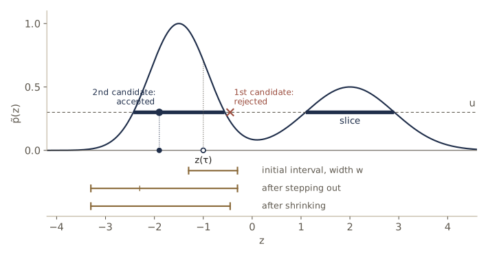
The first step is easy; the second is not, since we do not know where the slice ends, and for a multimodal density it can be several intervals. Instead of sampling the slice exactly, we make a move that leaves the uniform distribution on the slice invariant. The stepping-out and shrinkage procedure, for a width parameter \(w\):
- Stepping out. Place an interval of width \(w\) at a random offset around the current \(z\). While the left end is inside the slice, move it left by \(w\); same for the right end.
- Shrinkage. Draw \(z'\) uniformly from the interval. If \(z'\) is in the slice, accept it. If not, shrink the interval by moving the endpoint on the same side as \(z'\) to \(z'\) (the current \(z\) always stays inside), and draw again.
Neal shows that this procedure satisfies detailed balance with respect to the uniform distribution on the slice. The width \(w\) affects only efficiency: too small costs many stepping-out evaluations, too large costs a few shrinkage steps, and neither is catastrophic. Working with \(\ln \tilde{p}\) and \(\ln u = \ln \tilde{p}(z) + \ln(\text{uniform})\) avoids underflow.
def slice_sample(log_p, z0, w, n, rng):
    """1-D slice sampling with stepping out and shrinkage (Neal, 2003).
    Returns n samples and the average number of density evaluations per sample."""
    z, lp = z0, log_p(z0)
    out = np.empty(n)
    n_evals = 0
    for t in range(n):
        log_u = lp + math.log(rng.random())         # height u ~ U(0, p~(z)), in logs
        left = z - w * rng.random()                  # interval of width w around z
        right = left + w
        while log_p(left) > log_u:                   # step out to the left
            left -= w
            n_evals += 1
        while log_p(right) > log_u:                  # step out to the right
            right += w
            n_evals += 1
        n_evals += 2
        while True:                                  # shrink until a point in the slice
            z_new = rng.uniform(left, right)
            lp_new = log_p(z_new)
            n_evals += 1
            if lp_new > log_u:
                break
            if z_new < z:
                left = z_new
            else:
                right = z_new
        z, lp = z_new, lp_new
        out[t] = z
    return out, n_evals / n

def log_p_tilde_scalar(z):
    """log p~ for one float (plain math is faster than NumPy for scalars)."""
    return math.log(math.exp(-(z + 1.5)**2 / 0.72) + 0.5 * math.exp(-(z - 2.0)**2 / 1.62) + 1e-300)

p_right = 1 - p_cdf(0.25)                           # exact mass to the right of the dip
rng_sl = np.random.default_rng(1141)
print(f"exact: mean 0.0000  E[z^2] {true_m2:.4f}  P(z > 0.25) {p_right:.4f}")
for w in [0.1, 1.0, 10.0]:
    zs, ev = slice_sample(log_p_tilde_scalar, 0.0, w, 20_000, rng_sl)
    print(f"w = {w:4.1f}: mean {zs.mean():7.4f}  E[z^2] {np.mean(zs**2):.4f}  "
          f"P(z > 0.25) {np.mean(zs > 0.25):.4f}  evals/sample {ev:5.1f}  IAT {iat(zs):4.1f}")
exact: mean 0.0000  E[z^2] 3.5529  P(z > 0.25) 0.4185
w =  0.1: mean  0.0545  E[z^2] 3.5942  P(z > 0.25) 0.4309  evals/sample  34.5  IAT  9.6
w =  1.0: mean -0.0109  E[z^2] 3.5532  P(z > 0.25) 0.4159  evals/sample   6.7  IAT  6.3
w = 10.0: mean -0.0034  E[z^2] 3.5440  P(z > 0.25) 0.4193  evals/sample   5.3  IAT  2.1
All three widths give roughly the right answers, at different costs. With \(w = 0.1\) the stepping out takes many small steps, and the estimated probability of the right bump is off by more than the others: when the height \(u\) is above the dip between the bumps, the slice is two separate intervals, and stepping out in small increments stops at the edge of the current bump, so the chain changes bumps only when \(u\) happens to fall below the dip. With a larger \(w\) the interval often spans both bumps and the chain moves between them freely. (Slow switching between bumps is also the kind of behavior that a single-run autocorrelation estimate can understate, so treat the \(w = 0.1\) value of \(\tau\) with suspicion.)
For several variables, slice sampling can update one coordinate at a time, as in Gibbs sampling, using any function proportional to the full conditional \(p(z_i \mid \mathbf{z}_{\setminus i})\), which is just \(\tilde{p}(\mathbf{z})\) viewed as a function of \(z_i\).
Hybrid Monte Carlo
Random-walk behavior is the main weakness of Metropolis and Gibbs sampling. Hybrid Monte Carlo (Duane and coauthors, 1987), now usually called Hamiltonian Monte Carlo (HMC), avoids it by borrowing the equations of motion from classical mechanics. It makes long, directed moves that are nevertheless accepted with high probability. It needs the gradient of \(\ln \tilde{p}(\mathbf{z})\), so it applies to continuous variables with differentiable densities.
Dynamical systems
Write the target as
\[p(\mathbf{z}) = \frac{1}{Z_p} \exp\big(-E(\mathbf{z})\big),\]where \(E(\mathbf{z}) = -\ln \tilde{p}(\mathbf{z})\) is called the potential energy. Picture a frictionless particle sliding on the surface \(E(\mathbf{z})\): it speeds up going downhill and slows going uphill. To describe its motion, introduce a momentum variable \(r_i = dz_i / d\tau\) for each position variable \(z_i\), where \(\tau\) is now continuous time; together, \((\mathbf{z}, \mathbf{r})\) live in phase space. The force on the particle is the negative gradient of the potential, so \(dr_i/d\tau = -\partial E / \partial z_i\). Define the kinetic energy \(K(\mathbf{r}) = \frac{1}{2}\lVert \mathbf{r} \rVert^2 = \frac{1}{2}\sum_i r_i^2\) and the total energy, the Hamiltonian,
\[H(\mathbf{z}, \mathbf{r}) = E(\mathbf{z}) + K(\mathbf{r}).\]Since \(\partial H/\partial r_i = r_i\) and \(\partial H/\partial z_i = \partial E/\partial z_i\), the two equations of motion become Hamilton’s equations:
\[\frac{dz_i}{d\tau} = \frac{\partial H}{\partial r_i}, \qquad \frac{dr_i}{d\tau} = -\frac{\partial H}{\partial z_i}.\]Two properties of this dynamics matter for sampling.
Energy is conserved. By the chain rule and Hamilton’s equations,
\[\frac{dH}{d\tau} = \sum_i \left( \frac{\partial H}{\partial z_i} \frac{dz_i}{d\tau} + \frac{\partial H}{\partial r_i} \frac{dr_i}{d\tau} \right) = \sum_i \left( \frac{\partial H}{\partial z_i} \frac{\partial H}{\partial r_i} - \frac{\partial H}{\partial r_i} \frac{\partial H}{\partial z_i} \right) = 0.\]Volume is conserved (Liouville’s theorem). The dynamics moves every point of phase space with velocity \(\mathbf{V} = (d\mathbf{z}/d\tau, d\mathbf{r}/d\tau)\), and a flow preserves volume when this velocity field has zero divergence. It does:
\[\operatorname{div} \mathbf{V} = \sum_i \left( \frac{\partial}{\partial z_i} \frac{\partial H}{\partial r_i} - \frac{\partial}{\partial r_i} \frac{\partial H}{\partial z_i} \right) = 0,\]because mixed partial derivatives commute. A region of phase space may change shape as it flows, but not its volume.
Now consider the joint distribution on phase space
\[p(\mathbf{z}, \mathbf{r}) = \frac{1}{Z_H} \exp\big(-H(\mathbf{z}, \mathbf{r})\big) = \frac{1}{Z_p} e^{-E(\mathbf{z})} \cdot \frac{1}{(2\pi)^{D/2}} e^{-\lVert \mathbf{r} \rVert^2/2}.\]It factorizes: \(\mathbf{z}\) has our target distribution and \(\mathbf{r}\) is an independent standard Gaussian. The Hamiltonian flow leaves this distribution invariant: follow a small region for some time; its volume is unchanged and so is the value of \(H\) inside it, hence the probability it carries, density times volume, is unchanged. While \(H\) stays constant, \(\mathbf{z}\) and \(\mathbf{r}\) can change a great deal, so following the dynamics for a while moves \(\mathbf{z}\) far in a systematic way, with no random walk.
The flow alone is not ergodic, since it never changes \(H\). So we alternate it with a move that does: replace \(\mathbf{r}\) by a fresh draw from its conditional \(p(\mathbf{r} \mid \mathbf{z})\). Because \(\mathbf{r}\) and \(\mathbf{z}\) are independent, that conditional is just \(\mathcal{N}(\mathbf{0}, \mathbf{I})\), and the move is a Gibbs step, which leaves the joint distribution invariant.
Leapfrog integration
We cannot solve Hamilton’s equations exactly in general, so we integrate them numerically with a step size \(\epsilon\). The leapfrog scheme alternates momentum and position updates:
\[\begin{aligned} \widehat{r}_i(\tau + \epsilon/2) &= \widehat{r}_i(\tau) - \frac{\epsilon}{2} \frac{\partial E}{\partial z_i}\big(\widehat{\mathbf{z}}(\tau)\big), \\ \widehat{z}_i(\tau + \epsilon) &= \widehat{z}_i(\tau) + \epsilon\, \widehat{r}_i(\tau + \epsilon/2), \\ \widehat{r}_i(\tau + \epsilon) &= \widehat{r}_i(\tau + \epsilon/2) - \frac{\epsilon}{2} \frac{\partial E}{\partial z_i}\big(\widehat{\mathbf{z}}(\tau + \epsilon)\big). \end{aligned}\]A half step of momentum, a full step of position, another half step of momentum. When several leapfrog steps follow each other, the two half steps in the middle merge into one full momentum step, so a run of \(L\) leapfrog steps costs \(L\) gradient evaluations (plus one).
Leapfrog has two exact properties that ordinary integrators such as Euler’s method lack. Each of its three updates changes one set of variables by an amount that depends only on the other set, which shears phase space without changing volume, so leapfrog preserves volume exactly. And it is time-reversible: running \(L\) steps with step size \(-\epsilon\) (equivalently, negating the momentum and running forward) exactly undoes \(L\) steps with \(+\epsilon\). Energy, on the other hand, is conserved only approximately; the error shrinks as \(\epsilon^2\).
We check all three claims on the test Gaussian, for which \(E(\mathbf{z}) = \frac{1}{2}\mathbf{z}^{\mathrm{T}}\boldsymbol{\Lambda}\mathbf{z}\) and \(\nabla E = \boldsymbol{\Lambda}\mathbf{z}\), with \(\boldsymbol{\Lambda} = \boldsymbol{\Sigma}^{-1}\). We follow one trajectory for a fixed total time of 5, record the largest energy error, and compare with Euler’s method, which updates position and momentum simultaneously from the old values.
def E_gauss(z):
    """Potential energy -ln p~(z) of the test Gaussian, for each row of z."""
    return 0.5 * np.sum((z @ Lam_c) * z, axis=-1)

def grad_E_gauss(z):
    return z @ Lam_c                                 # Lambda is symmetric

def leapfrog(z, r, grad_E, eps, n_steps):
    """n_steps leapfrog steps of size eps (half momentum steps merged in the middle)."""
    r = r - 0.5 * eps * grad_E(z)
    for i in range(n_steps):
        z = z + eps * r
        if i < n_steps - 1:
            r = r - eps * grad_E(z)
    r = r - 0.5 * eps * grad_E(z)
    return z, r

def euler(z, r, eps):
    return z + eps * r, r - eps * grad_E_gauss(z)

def max_energy_error(step_fn, z, r, eps, t_total):
    """Largest |H - H(start)| along a trajectory of total time t_total."""
    H0 = E_gauss(z) + 0.5 * np.sum(r**2, axis=-1)
    err = 0.0
    for _ in range(int(round(t_total / eps))):
        z, r = step_fn(z, r, eps)
        err = max(err, float(np.max(np.abs(E_gauss(z) + 0.5 * np.sum(r**2, axis=-1) - H0))))
    return err

z_s, r_s = np.array([[1.0, 0.8]]), np.array([[0.5, -0.8]])
lf_step = lambda z, r, eps: leapfrog(z, r, grad_E_gauss, eps, 1)
print("   eps     leapfrog max|dH|    Euler max|dH|")
for eps in [0.2, 0.1, 0.05, 0.025, 0.0125]:
    print(f"{eps:7.4f}      {max_energy_error(lf_step, z_s, r_s, eps, 5.0):.2e}          "
          f"{max_energy_error(euler, z_s, r_s, eps, 5.0):.2e}")
for eps in [0.27, 0.29]:                                      # just below and above 2 sigma_min
    print(f"eps {eps}: leapfrog max|dH| over time 20 = {max_energy_error(lf_step, z_s, r_s, eps, 20.0):.2e}")

z_f, r_f = leapfrog(z_s, r_s, grad_E_gauss, 0.1, 50)          # 50 steps forward
z_b, r_b = leapfrog(z_f, -r_f, grad_E_gauss, 0.1, 50)         # flip momentum, 50 steps again
print(f"reversibility: max error in z {np.abs(z_b - z_s).max():.1e}, in r {np.abs(-r_b - r_s).max():.1e}")
   eps     leapfrog max|dH|    Euler max|dH|
 0.2000      1.73e-01          7.82e+11
 0.1000      6.29e-02          5.88e+08
 0.0500      1.57e-02          1.20e+05
 0.0250      3.94e-03          4.33e+02
 0.0125      9.84e-04          1.98e+01
eps 0.27: leapfrog max|dH| over time 20 = 4.33e+00
eps 0.29: leapfrog max|dH| over time 20 = 9.98e+26
reversibility: max error in z 7.8e-16, in r 3.3e-16
Once \(\epsilon\) is well inside the stability limit discussed below, each halving of \(\epsilon\) divides the leapfrog energy error by about 4, the \(\epsilon^2\) behavior. Euler’s method is useless here: along the stiff short axis of the ellipse its energy grows exponentially unless the step is tiny. Leapfrog returns to its starting point up to rounding error.
Watch out. Leapfrog is stable only if \(\epsilon\) is small compared with the shortest length scale of the target. For a Gaussian with smallest standard deviation \(\sigma_{\min}\), the limit is \(\epsilon < 2\sigma_{\min}\) (exercise 11); here \(2\sigma_{\min} \approx 0.283\), and the output above shows the energy error jumping by many orders of magnitude between \(\epsilon = 0.27\) and \(\epsilon = 0.29\). In a real model, a step size that is fine in most places can be unstable in a narrow region of the posterior, which shows up as a sudden drop in the acceptance rate.
Hybrid Monte Carlo
With a nonzero step size, leapfrog does not conserve \(H\) exactly, and without a correction the samples would be biased. HMC removes the bias with a Metropolis test on the total energy. One iteration:
- Draw a fresh momentum \(\mathbf{r} \sim \mathcal{N}(\mathbf{0}, \mathbf{I})\).
- Choose a direction at random: step size \(+\epsilon\) or \(-\epsilon\) with probability \(\frac{1}{2}\) each.
- Run \(L\) leapfrog steps from \((\mathbf{z}, \mathbf{r})\) to a candidate \((\mathbf{z}^\star, \mathbf{r}^\star)\).
- Accept \(\mathbf{z}^\star\) with probability \(\min\big(1, \exp\{H(\mathbf{z}, \mathbf{r}) - H(\mathbf{z}^\star, \mathbf{r}^\star)\}\big)\); otherwise keep \(\mathbf{z}\).
If leapfrog were exact, \(H\) would not change and every candidate would be accepted. With \(\epsilon\) well inside the stability limit, the energy error is small and so is the rejection rate, even for long trajectories.
Why it samples correctly. Leapfrog followed by the Metropolis test satisfies detailed balance for \(p(\mathbf{z}, \mathbf{r})\). Take a small region \(\mathcal{R}\) of phase space with volume \(\delta V\) that \(L\) forward leapfrog steps map to a region \(\mathcal{R}'\); by volume preservation, \(\mathcal{R}'\) also has volume \(\delta V\). The probability of starting in \(\mathcal{R}\), choosing the forward direction, and accepting the move to \(\mathcal{R}'\) is
\[\frac{1}{Z_H} e^{-H(\mathcal{R})}\, \delta V \cdot \frac{1}{2} \cdot \min\big(1, e^{H(\mathcal{R}) - H(\mathcal{R}')}\big) = \frac{\delta V}{2 Z_H} \min\big(e^{-H(\mathcal{R})}, e^{-H(\mathcal{R}')}\big).\]By reversibility, \(L\) backward steps map \(\mathcal{R}'\) exactly onto \(\mathcal{R}\), and the probability of that move is the same expression with \(\mathcal{R}\) and \(\mathcal{R}'\) swapped, which is equal because the minimum is symmetric. Both ingredients were needed: volume preservation lets us compare densities without a Jacobian factor, and reversibility supplies the reverse move. The momentum refresh is a Gibbs step, so the whole iteration leaves \(p(\mathbf{z}, \mathbf{r})\) invariant, and the \(\mathbf{z}\) samples come from \(p(\mathbf{z})\).
(Because the momentum is redrawn from a symmetric distribution, choosing the direction at random makes no difference to the distribution of the moves; we keep it to match the argument.) One more detail: for some targets, a fixed \(\epsilon\) and \(L\) can bring the trajectory back to where it started, and the chain would stop being ergodic. Drawing \(\epsilon\) at random from a small interval each iteration prevents this.
def hmc(E, grad_E, z0, eps, n_leap, n_iter, rng, jitter=0.2):
    """Hybrid (Hamiltonian) Monte Carlo on C chains at once. z0: (C, D).
    The step size is eps * U(1 - jitter, 1 + jitter) with a random sign, per chain and iteration."""
    z = np.array(z0, float)
    C, D = z.shape
    out = np.empty((n_iter, C, D))
    n_acc = 0
    for t in range(n_iter):
        r = rng.standard_normal((C, D))                          # Gibbs step for the momentum
        e = eps * (1 + jitter * (2 * rng.random(C) - 1)) * rng.choice([-1.0, 1.0], C)
        z_new, r_new = leapfrog(z, r, grad_E, e[:, None], n_leap)
        H_old = E(z) + 0.5 * np.sum(r**2, axis=1)
        H_new = E(z_new) + 0.5 * np.sum(r_new**2, axis=1)
        accept = np.log(rng.random(C)) < H_old - H_new            # min(1, exp(H - H*))
        z[accept] = z_new[accept]
        out[t] = z
        n_acc += accept.sum()
    return out, n_acc / (n_iter * C)

rng_h = np.random.default_rng(1151)
z0 = sample_gaussian(np.zeros(2), L_c, 20, rng_h)
print("  eps   L   accept   IAT (long axis)   ESS per 1000 gradients   mean                var")
for eps, n_leap in [(0.05, 40), (0.1, 10), (0.1, 20), (0.2, 10), (0.25, 10)]:
    s, acc = hmc(E_gauss, grad_E_gauss, z0, eps, n_leap, 1000, rng_h)
    tau = mean_iat(major_axis(s))
    print(f"{eps:5.2f}  {n_leap:3d}   {acc:.3f}      {tau:6.2f}              {1000 / (tau * n_leap):5.1f}"
          f"            {s.reshape(-1, 2).mean(axis=0)}   {s.reshape(-1, 2).var(axis=0)}")
  eps   L   accept   IAT (long axis)   ESS per 1000 gradients   mean                var
 0.05   40   0.994        1.52               16.4            [-0.0145 -0.0168]   [1.0058 1.0045]
 0.10   10   0.969        7.49               13.3            [ 0.0011 -0.001 ]   [1.0114 1.0155]
 0.10   20   0.974        1.49               33.5            [0.017  0.0165]   [0.9957 1.0028]
 0.20   10   0.861        1.83               54.7            [-0.0031 -0.0045]   [0.9921 0.9877]
 0.25   10   0.572        2.28               43.9            [0.0035 0.0038]   [1.0122 1.0129]
The means and variances are right (0 and 1), acceptance rates are high, and when the trajectory is long enough (about 2 time units or more) consecutive HMC samples are nearly independent: autocorrelation times of about 1.5 to 2.3 iterations, against about 50 sweeps for Gibbs and at least about 60 steps for the best random-walk Metropolis. The row with \(\epsilon = 0.1\) and \(L = 10\) shows the other side: a trajectory of total length 1 is too short to cross the long axis, and the autocorrelation time rises. Counting cost in gradient evaluations, the good settings here give about 33 to 55 effective samples per 1000 gradients, against at most about 16 effective samples per 1000 density evaluations for random-walk Metropolis. As \(\epsilon\) approaches the stability limit, acceptance falls.
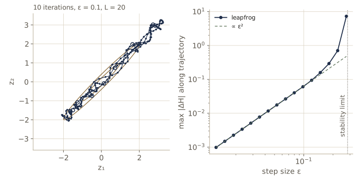
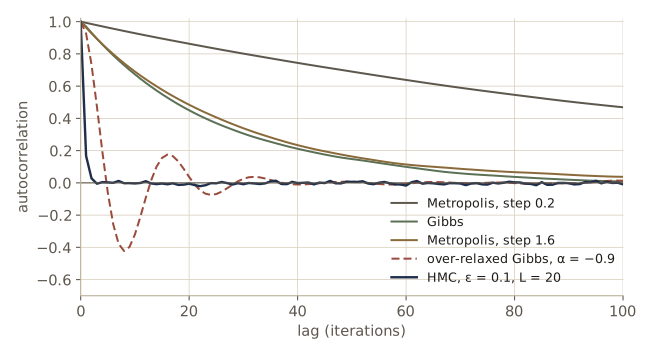
How HMC scales
Why the large difference? Consider a Gaussian with independent components of standard deviations \(\sigma_i\), so that \(H = \sum_i z_i^2/(2\sigma_i^2) + \sum_i r_i^2/2\); the conclusion carries over to correlated Gaussians because HMC treats all directions alike, and a rotation does not change it. During leapfrog, each pair \((z_i, r_i)\) evolves independently, as an oscillator with period \(2\pi\sigma_i\). For the integration to be accurate, \(\epsilon\) must be small compared with the smallest scale, \(\sigma_{\min}\); a large error in any single coordinate spoils the acceptance test for all of them. To move a distance comparable to \(\sigma_{\max}\) in the widest direction, the trajectory must last a time of order \(\sigma_{\max}\), which takes about \(\sigma_{\max}/\sigma_{\min}\) leapfrog steps. Random-walk Metropolis, with steps of size about \(\sigma_{\min}\), needs about \((\sigma_{\max}/\sigma_{\min})^2\) steps for the same distance.
HMC uses the gradient of \(\ln p\), which random-walk Metropolis ignores. A gradient in \(D\) dimensions carries \(D\) numbers of information and, with automatic differentiation, typically costs only a small constant factor more than evaluating \(\ln p\) itself, whatever \(D\) is. The same reasoning is why gradient-based optimizers usually beat derivative-free ones. HMC and its adaptive variants are the default samplers in widely used probabilistic programming systems.
Estimating the partition function
Every sampler in this module avoided the normalizing constant. Sometimes we need it anyway. For a distribution written as \(p_E(\mathbf{z}) = \exp(-E(\mathbf{z}))/Z_E\), the constant \(Z_E = \int \exp(-E(\mathbf{z}))\, d\mathbf{z}\) is called the partition function. For a posterior, it is the model evidence \(p(\mathcal{D})\), which Bayesian model comparison needs (module 03); in fact only ratios of evidences between models matter, multiplied by the ratio of their prior probabilities.
The importance-sampling identity from earlier estimates a ratio of partition functions. With a second distribution \(p_G(\mathbf{z}) = \exp(-G(\mathbf{z}))/Z_G\) that we can sample from,
\[\frac{Z_E}{Z_G} = \frac{\int \exp(-E(\mathbf{z}) + G(\mathbf{z}))\, \exp(-G(\mathbf{z}))\, d\mathbf{z}}{Z_G} = \mathbb{E}_{p_G}\big[\exp(-E + G)\big] \approx \frac{1}{L}\sum_{l=1}^{L} \exp\big(-E(\mathbf{z}^{(l)}) + G(\mathbf{z}^{(l)})\big),\]with \(\mathbf{z}^{(l)} \sim p_G\). If \(Z_G\) is known, as it is for a Gaussian, this gives \(Z_E\) itself.
To test it we need an \(E\) whose partition function we know. Take \(E(\mathbf{z}) = \frac{1}{4}\sum_{i=1}^{D} z_i^4\), a product of \(D\) identical one-dimensional factors. Substituting \(t = z^4/4\) in one dimension gives \(\int e^{-z^4/4}\, dz = \Gamma(\tfrac{1}{4})/\sqrt{2}\), so \(Z_E = \big(\Gamma(\tfrac{1}{4})/\sqrt{2}\big)^D\). The same substitution gives the variance of each coordinate, \(2\Gamma(\tfrac{3}{4})/\Gamma(\tfrac{1}{4}) \approx 0.676\). For \(G\) we try two isotropic Gaussians: one with this matched variance, and a standard Gaussian.
Z1 = np.exp(gammaln(0.25)) / np.sqrt(2)                      # exact 1-D partition function
var_matched = 2 * np.exp(gammaln(0.75) - gammaln(0.25))      # variance of p_E per coordinate

def log_Z_is(D, s2, L, rng):
    """Importance-sampling estimate of ln Z_E with G(z) = ||z||^2 / (2 s2); also the IS ESS."""
    z = np.sqrt(s2) * rng.standard_normal((L, D))
    log_r = -np.sum(z**4, axis=1) / 4 + np.sum(z**2, axis=1) / (2 * s2)    # -E + G
    log_ZG = 0.5 * D * np.log(2 * np.pi * s2)
    w = np.exp(log_r - logsumexp(log_r))
    return log_ZG + logsumexp(log_r) - np.log(L), 1 / np.sum(w**2)

rng_z = np.random.default_rng(1161)
print(f"var of p_E per coordinate: {var_matched:.4f}")
print("   D    Z_E estimate / exact        IS ESS (of 40000)")
print("        matched G  standard G     matched  standard")
for D in [1, 10, 50, 200]:
    (lm, em), (ls, es) = [log_Z_is(D, s2, 40_000, rng_z) for s2 in (var_matched, 1.0)]
    exact_log = D * np.log(Z1)
    print(f"{D:4d}     {np.exp(lm - exact_log):.4f}     {np.exp(ls - exact_log):.4f}      "
          f"{em:7.0f}   {es:7.0f}")
var of p_E per coordinate: 0.6760
   D    Z_E estimate / exact        IS ESS (of 40000)
        matched G  standard G     matched  standard
   1     1.0001     1.0007        37954     36859
  10     1.0012     1.0020        23472     17550
  50     1.0298     1.0168         2758       517
 200     1.1390     0.2898           40         2
In low dimensions either \(G\) works. As \(D\) grows, the mismatch between \(p_E\) and \(p_G\) compounds across coordinates and the weights become dominated by a few samples. With the standard Gaussian in 200 dimensions, the estimate is off by a factor of more than three, and the effective sample size is 2 out of 40,000. The matched Gaussian lasts longer, but at \(D = 200\) it too is off by more than 10%, with an effective sample size of 40. Since \(Z_E\) is a product over coordinates, a small per-coordinate mismatch becomes an exponentially large one.
Two refinements address this (Bishop §11.6 gives the details). When no simple \(p_G\) matches well, the samples of a Markov chain can define one: with transition probabilities \(T\) and chain states \(\mathbf{z}^{(1)}, \dots, \mathbf{z}^{(L)}\), the mixture \(\frac{1}{L}\sum_l T(\mathbf{z}^{(l)}, \mathbf{z})\) is a normalized density that follows the target and can serve as \(p_G\). And rather than bridge a large gap in one step, chaining introduces intermediate distributions \(p_1, p_2, \dots, p_M\) between a simple \(p_1\) with known \(Z_1\) and the target \(p_M\), and multiplies ratios that are each easy to estimate:
\[\frac{Z_M}{Z_1} = \frac{Z_2}{Z_1} \cdot \frac{Z_3}{Z_2} \cdots \frac{Z_M}{Z_{M-1}}.\]A convenient family interpolates the energies, \(E_\alpha(\mathbf{z}) = (1 - \alpha) E_1(\mathbf{z}) + \alpha E_M(\mathbf{z})\) for \(0 \le \alpha \le 1\). The samples for each stage come from MCMC, and a single chain can move through the sequence as \(\alpha\) increases, provided it stays close to equilibrium at every stage.
Summary
| Method | What it needs | What it produces | Main limitation |
|---|---|---|---|
| Transformation (inverse CDF, Box–Muller, Cholesky) | an invertible CDF or a known construction | exact independent samples | only standard distributions |
| Rejection sampling | \(\tilde{p}\); a proposal \(q\) and \(k\) with \(kq \ge \tilde{p}\) | exact independent samples; acceptance \(Z_p/k\) | acceptance falls exponentially with dimension |
| Adaptive rejection sampling | log-concave \(\tilde{p}\) (and its derivative) | exact samples, envelope refined on the fly | one-dimensional, log-concave |
| Importance sampling | \(\tilde{p}\); a proposal \(q\) | weighted samples, expectations, \(Z_p/Z_q\) | fails silently if \(q\) misses mass of \(p\) |
| Sampling-importance-resampling | as importance sampling | approximate unweighted samples | exact only as \(L \to \infty\) |
| Metropolis–Hastings | \(\tilde{p}\); a proposal \(q(\mathbf{z}^\star \mid \mathbf{z})\) | correlated samples from a Markov chain | random walk: \((\sigma_{\max}/\sigma_{\min})^2\) steps |
| Gibbs sampling | samplers for the full conditionals | correlated samples, no rejections | slow when variables are strongly dependent |
| Slice sampling | \(\tilde{p}\) | correlated samples, self-tuning step | multivariate use is one coordinate at a time |
| Hybrid (Hamiltonian) Monte Carlo | \(\tilde{p}\) and \(\nabla \ln \tilde{p}\) | correlated samples with long moves | tuning \(\epsilon\) and \(L\); continuous variables only |
Ideas to carry forward:
- A Monte Carlo estimate has error \(\sqrt{\tau \operatorname{var}[f] / L}\), independent of dimension. All the difficulty is in producing samples, and \(\tau\), the integrated autocorrelation time, is the honest measure of a sampler’s quality: report effective sample sizes, not chain lengths.
- Methods with a fixed proposal (rejection, importance) break down in high dimensions because the proposal and the target stop overlapping. Markov chains fix this by proposing locally, at the price of correlated samples.
- Detailed balance is the design principle behind Metropolis–Hastings, Gibbs, slice sampling, and HMC: each move leaves the target invariant, and ergodicity makes the chain forget its start.
- Random walks are slow. Over-relaxation, blocking, and above all Hamiltonian dynamics make progress by moving in consistent directions; HMC uses gradient information to do so.
Exercises
- For the AR(1) sequence \(z_l = \rho z_{l-1} + \sqrt{1-\rho^2}\,\epsilon_l\) in equilibrium, show that \(\operatorname{cov}[z_l, z_{l+k}] = \rho^{k}\), and compute \(\operatorname{var}[\widehat{f}]\) for \(f(z) = z\) exactly for finite \(L\). Show that \(L \operatorname{var}[\widehat{f}] \to (1+\rho)/(1-\rho)\) as \(L \to \infty\). What happens for negative \(\rho\), and why is that interesting?
- The Laplace distribution has density \(p(y) = \frac{1}{2b} e^{-\lvert y - m \rvert / b}\). Derive its CDF and the inverse, write
sample_laplace(m, b, L, rng), and check it with moments and a KS test againststats.laplace. - Complete the Jacobian proof of the Box–Muller method: with \((z_1, z_2)\) uniform on the unit disk, compute \(\partial(z_1, z_2)/\partial(y_1, y_2)\) and show that the joint density of \((y_1, y_2)\) is a product of two standard Gaussian densities. (Working with the inverse map is easier.)
- Write a rejection sampler for the gamma distribution \(\operatorname{Gam}(z \mid a, 1)\) with \(a = 3\), using a Cauchy proposal with location \(c\) and scale \(s\) sampled by
sample_cauchy. Find \(k\) numerically for a few choices of \((c, s)\) and report the acceptance rates. How close to optimal is \(c = a - 1\), \(s = \sqrt{2a - 1}\)? Check the samples with a KS test. - Repair the failing importance sampler of this module with a defensive mixture proposal that puts weight 0.5 on \(\mathcal{N}(-1.5, 0.4^2)\) and 0.5 on \(\mathcal{N}(0, 3^2)\). Estimate \(\mathbb{E}[z]\), \(\mathbb{E}[z^2]\), and \(Z_p\) over 50 independent runs and compare the spread of the estimates with those from the two single proposals. Explain why a heavy-tailed component bounds the weights.
- An independence sampler is Metropolis–Hastings with a proposal \(q(\mathbf{z}^\star)\) that ignores the current state. Write its acceptance probability in terms of the importance weights \(\tilde{r}(\mathbf{z}) = \tilde{p}(\mathbf{z})/q(\mathbf{z})\), implement it for the two-bump target with \(q = \mathcal{N}(0, 3^2)\), and compare its autocorrelation time with slice sampling. What happens with the narrow proposal \(\mathcal{N}(-1.5, 0.4^2)\)?
- Construct a three-state chain whose invariant distribution is uniform but which does not satisfy detailed balance. (Hint: a chain that prefers to move “clockwise”.) Verify both properties numerically and simulate it to confirm that it is still ergodic.
- Let \(p(z_1, z_2)\) be uniform on the union of the squares \([0, 1]^2\) and \([2, 3]^2\). Show that the Gibbs sampler started in one square never reaches the other, so the chain is not ergodic even though \(p\) is invariant. Propose a change of variables, or a different Metropolis–Hastings move, that fixes the problem, and demonstrate it in code.
- Implement random-scan Gibbs sampling for the correlated Gaussian (at each step update \(z_1\) or \(z_2\), chosen with probability \(\frac{1}{2}\)). Compare the autocorrelation time per coordinate update with systematic-scan Gibbs, and explain the difference in terms of the AR(1) argument.
- Use
slice_samplecoordinate by coordinate to sample the correlated Gaussian (each full conditional is a 1-D Gaussian known up to a constant). Measure the autocorrelation time per sweep and compare it with Gibbs sampling. Then do the same for the posterior of \((\mu, \lambda)\) in the Gibbs example, without using the gamma and Gaussian forms of the conditionals. - For \(E(z) = z^2/(2\sigma^2)\) in one dimension, show that one leapfrog step is a linear map \((z, r) \mapsto \mathbf{A}(z, r)\). Compute \(\mathbf{A}\), show that \(\det \mathbf{A} = 1\) (volume preservation), and show that its eigenvalues have modulus 1 when \(\epsilon < 2\sigma\) and one has modulus greater than 1 when \(\epsilon > 2\sigma\). Relate this to the stability limit in the module.
- Extend the partition-function experiment with chaining: for \(D = 200\), use intermediate energies \(E_\alpha = (1-\alpha) G + \alpha E\) for \(\alpha\) on a grid of 20 values, draw samples at each stage with a few steps of random-walk Metropolis or HMC started from the previous stage’s samples, and multiply the estimated ratios. Compare with the single-step estimate using the standard Gaussian.
- In your own words: explain to a classmate why a Markov chain sampler with a 98% acceptance rate can be worse than one with a 10% acceptance rate, and what number you would look at instead to judge a sampler.
Going further
- Bishop, Pattern Recognition and Machine Learning, chapter 11 — the source for this module. Exercises 11.2–11.5 are about the transformation method and Box–Muller, 11.6 is the correctness of rejection sampling, 11.8–11.9 build the adaptive rejection envelope, 11.11–11.13 are about Gibbs sampling (11.13 is the normal mean and precision model), and 11.15–11.17 work through Hamiltonian dynamics and detailed balance for hybrid Monte Carlo.
- N. Metropolis, A. W. Rosenbluth, M. N. Rosenbluth, A. H. Teller, and E. Teller, “Equation of state calculations by fast computing machines”, Journal of Chemical Physics, 1953, and W. K. Hastings, “Monte Carlo sampling methods using Markov chains and their applications”, Biometrika, 1970 — the two papers behind Metropolis–Hastings.
- Radford M. Neal, “Slice sampling”, Annals of Statistics, 2003 — stepping out, doubling, shrinkage, and multivariate versions, with the correctness proofs.
- Radford M. Neal, “MCMC using Hamiltonian dynamics”, a chapter of the Handbook of Markov Chain Monte Carlo (2011) — the clearest account of HMC, its tuning, and its scaling.
- David J. C. MacKay, Information Theory, Inference, and Learning Algorithms (Cambridge University Press, 2003; free online from the author), chapters 29 and 30 — Monte Carlo methods and efficient samplers, with many pictures.
- Charles J. Geyer, “Practical Markov chain Monte Carlo”, Statistical Science, 1992 — practical advice on running chains, including the pairwise rule for estimating autocorrelation times used in this module.
These notes follow the chapters of C. M. Bishop, Pattern Recognition and Machine Learning (Springer, 2006), the course text, which Microsoft Research makes freely available as a PDF. The explanations, code, figures, and exercises here are written for this course; the book remains the reference, with the full derivations and many more exercises.