CSE 474/574 · Module 09 · Week 10
Mixture Models and EM
K-means, Gaussian mixtures, the EM algorithm and why it works, Bernoulli mixtures, and EM as coordinate ascent on a lower bound.
Companion reading: Bishop, Pattern Recognition and Machine Learning, chapter 9, “Mixture Models and EM”
By the end of this module you can
- Write down the K-means distortion, derive both K-means steps as exact minimizations, and explain why the algorithm stops in finitely many steps but only at a local minimum.
- Use K-means for vector quantization of an image and count the bits a codebook saves.
- Describe a Gaussian mixture as a latent-variable model with a 1-of-K variable, sample from it, and compute responsibilities in log space.
- Explain the singularities and the K! symmetry of the Gaussian-mixture likelihood, and say what to do about the singularities.
- Derive the EM updates for a Gaussian mixture and implement EM so that the log-likelihood never decreases.
- State EM in terms of the expected complete-data log-likelihood and apply it to Bernoulli mixtures and to the hyperparameters of Bayesian linear regression.
- Show that K-means is the small-variance limit of EM for a Gaussian mixture.
- Prove the decomposition \(\ln p(\mathbf{X} \mid \boldsymbol{\theta}) = \mathcal{L}(q, \boldsymbol{\theta}) + \mathrm{KL}(q \Vert p)\) and use it to explain why EM works and how its MAP, generalized, and incremental variants follow.
Contents
- K-means clustering
- Image segmentation and compression
- Mixtures of Gaussians
- An alternative view of EM
- The EM algorithm in general
- Summary
- Exercises
- Going further
In module 02 we met the Gaussian mixture as a density: a weighted sum of \(K\) Gaussian bumps, flexible enough to imitate almost any smooth density. We wrote it down, but we never fit one to data. The reason is that the maximum likelihood equations for a mixture have no closed-form solution. This module supplies the tool that fits it.
The tool rests on one move: add variables we never observe. Suppose each data point came with a hidden label that says which bump produced it. With the labels in hand, fitting is easy, because we fit one Gaussian to each group. Without them, we alternate. We guess the labels, softly, from the current parameters; then we refit the parameters as if the guesses were data; and we repeat. That alternation is the expectation–maximization (EM) algorithm. It is not limited to Gaussian mixtures: hidden Markov models (module 13), probabilistic PCA (module 12), and the hyperparameters \(\alpha\) and \(\beta\) of Bayesian linear regression from module 03 all yield to it.
We start with no probability at all, with the K-means clustering algorithm, which already has the two-step shape of EM. Then we build the Gaussian mixture as a latent-variable model and derive EM for it. We then look at the same algorithm twice more: as maximizing an expected complete-data log-likelihood, and as coordinate ascent on a lower bound of the log-likelihood. That lower bound is the doorway to the variational inference of module 10.
K-means clustering
The distortion measure
We have \(N\) points \(\mathbf{x}_1, \dots, \mathbf{x}_N\) in \(\mathbb{R}^D\) and want to split them into \(K\) groups, or clusters, so that points in the same cluster are close to each other. For now \(K\) is given.
Give each cluster a prototype \(\boldsymbol{\mu}_k \in \mathbb{R}^D\), a representative point that we will soon see is the cluster’s center. Record which cluster each point belongs to with binary indicators \(r_{nk} \in \{0, 1\}\): \(r_{nk} = 1\) if point \(n\) is in cluster \(k\), and exactly one of \(r_{n1}, \dots, r_{nK}\) equals 1. This way of writing a choice among \(K\) options as a binary vector with a single 1 is called 1-of-K coding (in machine learning code it is usually called one-hot encoding).
Definition. The distortion of an assignment \(\{r_{nk}\}\) and prototypes \(\{\boldsymbol{\mu}_k\}\) is the total squared distance from every point to the prototype of its cluster, \(J = \sum_{n=1}^{N} \sum_{k=1}^{K} r_{nk} \lVert \mathbf{x}_n - \boldsymbol{\mu}_k \rVert^2\). K-means clustering looks for the assignment and prototypes that make \(J\) small.
Minimizing \(J\) over both sets of unknowns at once is hard: the assignments are discrete, and there are \(K^N\) of them. But each half of the problem, with the other half held fixed, is easy.
Two easy half-problems
Assignments with the prototypes fixed. With the \(\boldsymbol{\mu}_k\) fixed, \(J\) is a sum of separate terms, one per data point, and the term for point \(n\) is \(\sum_k r_{nk} \lVert \mathbf{x}_n - \boldsymbol{\mu}_k \rVert^2\). Only one \(r_{nk}\) can be 1, so the best choice puts the 1 at the nearest prototype:
\[r_{nk} = \begin{cases} 1 & \text{if } k = \arg\min_j \lVert \mathbf{x}_n - \boldsymbol{\mu}_j \rVert^2, \\ 0 & \text{otherwise.} \end{cases}\]Prototypes with the assignments fixed. With the \(r_{nk}\) fixed, \(J\) is a convex quadratic function of each \(\boldsymbol{\mu}_k\) separately. Its gradient with respect to \(\boldsymbol{\mu}_k\) is \(-2 \sum_n r_{nk} (\mathbf{x}_n - \boldsymbol{\mu}_k)\), and setting it to zero gives
\[\boldsymbol{\mu}_k = \frac{\sum_n r_{nk} \mathbf{x}_n}{\sum_n r_{nk}},\]the mean of the points currently assigned to cluster \(k\). That is where the name comes from: the prototypes are \(K\) means.
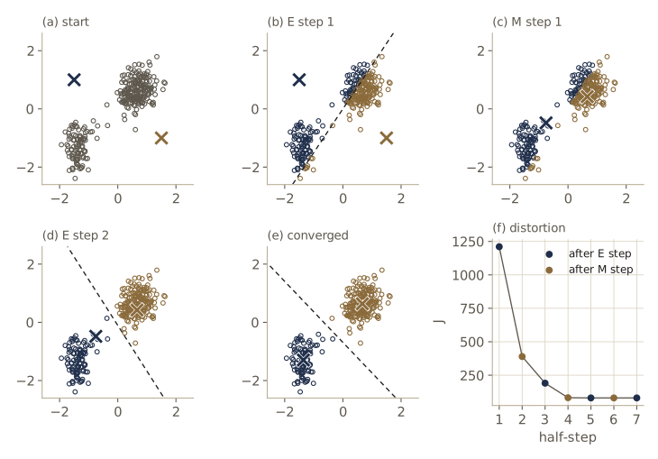
The K-means algorithm starts from some initial prototypes and alternates the two updates until the assignments stop changing. Alternately minimizing a function over one block of variables while the other block is held fixed is called coordinate descent. We will call the assignment update the E step and the prototype update the M step; the names will make sense once we meet EM, of which this is a special case.
Why does it stop? Each half-step minimizes \(J\) exactly over its block, so \(J\) never increases. The assignments can take only finitely many values, and each assignment determines the M-step prototypes uniquely. So as long as the assignments keep changing, \(J\) must keep strictly decreasing (ignoring exact ties in distance, which a fixed tie-breaking rule handles), which means no assignment can come back, and the algorithm must stop after finitely many steps. What it cannot promise is that the stopping point is the global minimum of \(J\): it is only a point that neither half-step can improve.
With two prototypes, “assign each point to the nearer prototype” splits the plane along the perpendicular bisector of the segment joining them. With \(K\) prototypes, the regions of points nearest to each prototype are convex polygons (in higher dimensions, polytopes), the Voronoi cells of the prototypes. The E step colors each cell; the M step moves each prototype to the center of mass of its cell’s points.
Running K-means
We need data with visible clusters. We generate our own version of a classic shape: the Old Faithful geyser measurements, eruption length and the waiting time to the next eruption, both in minutes, which form two elongated clusters (short eruptions with short waits, long eruptions with long waits). Our 300 points come from two correlated Gaussians that we choose. Because the two columns have very different scales, we standardize them first: subtract each column’s mean and divide by its standard deviation, so that both measurements count equally in the Euclidean distance.
import numpy as np
from itertools import permutations
from scipy.special import logsumexp
from scipy.linalg import solve_triangular, cho_factor, cho_solve
from scipy.stats import multivariate_normal

np.set_printoptions(precision=4, suppress=True)
rng = np.random.default_rng(9)

def make_geyser(n, rng):
    """Synthetic (eruption length, waiting time) pairs in minutes: two clusters."""
    short = rng.random(n) < 0.35
    X = np.empty((n, 2))
    X[short] = rng.multivariate_normal([2.0, 54.5], [[0.07, 0.35], [0.35, 34.0]],
                                       size=short.sum())
    X[~short] = rng.multivariate_normal([4.3, 80.0], [[0.17, 0.95], [0.95, 36.0]],
                                        size=(~short).sum())
    return X, (~short).astype(int)          # label 0 = short cluster, 1 = long

X_raw, z_true = make_geyser(300, rng)
X = (X_raw - X_raw.mean(axis=0)) / X_raw.std(axis=0)     # standardize each column
N, D = X.shape
print("N =", N, " D =", D, f"  fraction in the long cluster: {z_true.mean():.3f}")
print("raw means:", X_raw.mean(axis=0), "  raw standard deviations:", X_raw.std(axis=0))
N = 300  D = 2   fraction in the long cluster: 0.673
raw means: [ 3.5472 72.0213]   raw standard deviations: [ 1.138  13.4453]
The implementation follows the two updates line by line. kmeans records \(J\) after every half-step so that we can watch it fall. If a cluster ever loses all its points, its prototype simply stays where it was.
def sq_dists(X, mu):
    """(N, K) matrix of squared distances between the rows of X and the rows of mu."""
    return ((X[:, None, :] - mu[None, :, :]) ** 2).sum(axis=-1)

def distortion(X, r, mu):
    """J for hard assignments r (an array of cluster indices 0..K-1)."""
    return ((X - mu[r]) ** 2).sum()

def kmeans_e_step(X, mu):
    return sq_dists(X, mu).argmin(axis=1)          # nearest prototype for every point

def kmeans_m_step(X, r, mu_old):
    mu = mu_old.copy()
    for k in range(len(mu)):
        if np.any(r == k):                 # an empty cluster keeps its old prototype
            mu[k] = X[r == k].mean(axis=0)
    return mu

def kmeans(X, mu, max_iter=300):
    """Batch K-means from initial prototypes mu.
    Returns prototypes, assignments, and J after each half-step."""
    J_hist, r = [], None
    for it in range(max_iter):
        r_new = kmeans_e_step(X, mu)
        J_hist.append(distortion(X, r_new, mu))
        if r is not None and np.array_equal(r_new, r):
            break                                  # assignments unchanged: converged
        r = r_new
        mu = kmeans_m_step(X, r, mu)
        J_hist.append(distortion(X, r, mu))
    return mu, r, J_hist
We start from two deliberately poor prototypes, placed off to the sides of the data, so that the algorithm has some work to do.
mu_init = np.array([[-1.5, 1.0], [1.5, -1.0]])      # a deliberately poor start
mu_km, r_km, J_hist = kmeans(X, mu_init)
for i, J in enumerate(J_hist):
    step = "E" if i % 2 == 0 else "M"
    print(f"after {step} step {i // 2 + 1}: J = {J:8.2f}")
print("J never increases:", bool(np.all(np.diff(J_hist) <= 1e-9)))
print("prototypes:\n", mu_km, "\ncluster sizes:", np.bincount(r_km))
after E step 1: J =  1210.35
after M step 1: J =   389.45
after E step 2: J =   190.23
after M step 2: J =    81.67
after E step 3: J =    80.06
after M step 3: J =    80.02
after E step 4: J =    80.02
J never increases: True
prototypes:
 [[-1.3573 -1.2949]
 [ 0.6685  0.6378]]
cluster sizes: [ 99 201]
The first E step, with the prototypes far from the data, has a large distortion. The first M step cuts it by more than half, because moving each prototype into the middle of its points is a big improvement. After three rounds the assignments settle, the last E step changes nothing, and the algorithm stops at \(J \approx 80\). The two clusters have 99 and 201 points. The data were generated with 98 short and 202 long eruptions, so K-means puts just one point on the wrong side.
Initialization and restarts
Because K-means only finds a local minimum, where it ends up depends on where it starts. A common and sensible start is to use \(K\) distinct data points, chosen at random, as the initial prototypes. Since each run is cheap, we run several random starts and keep the one with the lowest distortion.
Two clusters are too easy to show the problem, so here is a data set of five round blobs, three in a row and two above them, clustered with \(K = 5\) from ten random starts.
blob_rng = np.random.default_rng(21)
centers = np.array([[0, 0], [3, 0], [6, 0], [1.5, 2.6], [4.5, 2.6]])
X_blobs = np.vstack([c + 0.6 * blob_rng.standard_normal((60, 2)) for c in centers])

init_rng = np.random.default_rng(3)
finals = []
for restart in range(10):
    mu0 = X_blobs[init_rng.choice(len(X_blobs), size=5, replace=False)]  # 5 data points
    _, _, hist = kmeans(X_blobs, mu0)
    finals.append(hist[-1])
print("final J of the 10 starts:", np.round(finals, 1))
print(f"best {min(finals):.1f}, worst {max(finals):.1f}")
final J of the 10 starts: [190.2 190.2 190.2 419.5 190.2 190.2 190.2 419.5 190.2 190.2]
best 190.2, worst 419.5
Eight of the ten starts find the natural solution, one prototype per blob, with \(J = 190.2\). The other two stop at \(J = 419.5\), with two prototypes sharing one blob and a single prototype stretched over two blobs; no single reassignment or recentering can repair that, so K-means is stuck. Several restarts cost little and protect against such outcomes. A popular refinement, k-means++ (Arthur and Vassilvitskii, 2007), chooses the random starting points one at a time, favoring points far from the prototypes already chosen, which makes bad starts much less likely.
Each K-means iteration computes all \(NK\) point-to-prototype distances, so it costs \(O(NKD)\) time. For large data sets there are faster versions that organize the points in a tree or use the triangle inequality to skip distances that cannot matter; Bishop §9.1 has references.
Online K-means
The batch algorithm needs all the data at every step. When points arrive one at a time, we can instead move the nearest prototype a little toward each new point:
\[\boldsymbol{\mu}_k^{\mathrm{new}} = \boldsymbol{\mu}_k^{\mathrm{old}} + \eta_n \left( \mathbf{x}_n - \boldsymbol{\mu}_k^{\mathrm{old}} \right),\]where \(k\) is the prototype nearest to \(\mathbf{x}_n\) and \(\eta_n\) is a step size that shrinks over time. This is the Robbins–Monro sequential estimation of module 02 applied to the stationarity condition of the M step. With \(\eta_n = 1 / (\text{number of points prototype } k \text{ has absorbed})\) the update keeps \(\boldsymbol{\mu}_k\) equal to the running mean of the points assigned to it so far.
def online_kmeans(X, mu, rng, passes=1):
    """Sequential K-means: one point at a time, step 1 / (points absorbed so far)."""
    mu = mu.astype(float).copy()
    counts = np.zeros(len(mu))
    for _ in range(passes):
        for n in rng.permutation(len(X)):
            k = np.argmin(((X[n] - mu) ** 2).sum(axis=1))      # nearest prototype
            counts[k] += 1
            mu[k] += (X[n] - mu[k]) / counts[k]
    return mu

for passes in [1, 3]:
    mu_on = online_kmeans(X, mu_init, np.random.default_rng(0), passes)
    J_on = distortion(X, kmeans_e_step(X, mu_on), mu_on)
    gap = np.abs(mu_on - mu_km).max()
    print(f"{passes} pass(es): J = {J_on:.3f}, max gap to batch prototypes {gap:.3f}")
print(f"batch K-means:  J = {J_hist[-1]:.3f}")
1 pass(es): J = 80.019, max gap to batch prototypes 0.000
3 pass(es): J = 80.019, max gap to batch prototypes 0.000
batch K-means:  J = 80.019
With two well-separated clusters, a single pass already reproduces the batch prototypes to three decimals, and further passes change nothing visible. The online version never holds more than one point in memory, which is what makes it useful for data streams. With overlapping clusters or a constant step size, the online prototypes keep jittering around the batch solution instead (exercise 2).
K-medoids
K-means measures dissimilarity by squared Euclidean distance. That is a poor fit for categorical variables, and it makes the means sensitive to outliers: one far-away point drags a mean a long way. The K-medoids algorithm replaces the squared distance by a general dissimilarity \(\mathcal{V}(\mathbf{x}, \mathbf{x}')\) and minimizes \(\tilde{J} = \sum_n \sum_k r_{nk} \mathcal{V}(\mathbf{x}_n, \boldsymbol{\mu}_k)\).
The E step is unchanged: assign each point to the least dissimilar prototype. The M step can be hard for a general \(\mathcal{V}\), so K-medoids usually requires each prototype to be one of the data points in its cluster, called a medoid. The M step then tries every member of cluster \(k\) as the prototype and keeps the one with the smallest total dissimilarity to the other members, which costs \(O(N_k^2)\) evaluations of \(\mathcal{V}\) for a cluster of \(N_k\) points. It works for any dissimilarity we can evaluate.
Here we add six wild points to the geyser data and compare how far the K-means prototypes and the K-medoids prototypes (with the Manhattan distance) move.
def kmedoids(X, idx, V, max_iter=50):
    """K-medoids with dissimilarity V(A, B) -> matrix; prototypes are points X[idx]."""
    idx = np.array(idx)
    for _ in range(max_iter):
        r = V(X, X[idx]).argmin(axis=1)                        # E step
        new_idx = idx.copy()
        for k in range(len(idx)):  # M step: best member of each cluster
            members = np.flatnonzero(r == k)
            cost = V(X[members], X[members]).sum(axis=0)
            new_idx[k] = members[cost.argmin()]
        if np.array_equal(new_idx, idx):
            break
        idx = new_idx
    return idx

def manhattan(A, B):
    return np.abs(A[:, None, :] - B[None, :, :]).sum(axis=-1)

X_out = np.vstack([X, np.full((6, 2), 8.0)])  # six wild points far from both clusters
start = [np.argmax(z_true == 0), np.argmax(z_true == 1)]
mu_out, _, _ = kmeans(X_out, mu_init)
med_clean = kmedoids(X, start, manhattan)
med_out = kmedoids(X_out, start, manhattan)
print("K-means prototypes moved by:  ", np.linalg.norm(mu_out - mu_km, axis=1))
moved = np.linalg.norm(X_out[med_out] - X[med_clean], axis=1)
print("K-medoids prototypes moved by:", moved)
K-means prototypes moved by:   [0.     0.3012]
K-medoids prototypes moved by: [0. 0.]
The six outliers join the long cluster. They pull that cluster’s mean by 0.3 standard deviations toward themselves, while its medoid, which must be a member of the cluster with small total distance to the others, does not move at all.
One feature of every method so far is that each point belongs to exactly one cluster. A point halfway between two prototypes is assigned just as firmly as a point sitting on top of one. The probabilistic model of the next sections replaces these hard assignments with probabilities that express how unsure we are.
Image segmentation and compression
An image is a grid of pixels, and each pixel has a color given by three intensities, red, green, and blue, each in \([0, 1]\). If we forget where the pixels are and treat each one as a point in the three-dimensional color space, K-means groups the pixels into \(K\) colors. Repainting every pixel with its prototype gives an image that uses a palette of only \(K\) colors.
This is a crude form of image segmentation, the task of dividing an image into regions that look uniform or belong to one object. It is crude because it ignores position entirely: two pixels of the same color end up in the same segment however far apart they are. But it shows K-means at work on real-looking data, and it leads to compression.
Lossless compression lets us rebuild the data exactly; lossy compression accepts some error in return for a smaller representation. K-means gives a lossy scheme called vector quantization. We store the \(K\) prototypes, here called code-book vectors, and for each data point only the index of its nearest code-book vector. A new point is compressed the same way, by finding its nearest code-book vector.
Suppose the image has \(N\) pixels and each channel is stored with 8 bits. Sending it directly costs \(24N\) bits. Sending the code book costs \(24K\) bits, and a fixed-length index needs \(\lceil \log_2 K \rceil\) bits per pixel, so the compressed image costs
\[24K + N \lceil \log_2 K \rceil \ \text{bits}.\]We synthesize a small landscape, 120 by 180 pixels: a sky that fades from blue toward orange, a sun, two hills, and a house with a roof, plus some pixel noise so that the colors are not exactly uniform.
def make_image(h, w, rng):
    """A small synthetic landscape: smooth color regions plus pixel noise."""
    yy, xx = np.mgrid[0:h, 0:w] / np.array([h, w])[:, None, None]
    img = (np.array([0.55, 0.72, 0.90]) * (1 - 0.35 * yy[..., None])     # sky, fading
           + np.array([0.95, 0.80, 0.60]) * 0.35 * yy[..., None])
    sun = (xx - 0.75) ** 2 + ((yy - 0.25) * h / w) ** 2 < 0.012
    far_hill = yy > 0.62 + 0.10 * np.sin(2 * np.pi * xx * 1.2 + 0.5)
    near_hill = yy > 0.78 + 0.06 * np.sin(2 * np.pi * xx * 2.1 + 2.0)
    house = (xx > 0.18) & (xx < 0.32) & (yy > 0.52) & (yy < 0.72)
    roof = (yy > 0.40) & (yy <= 0.52) & (np.abs(xx - 0.25) < (yy - 0.40) * 0.9)
    img[sun] = [0.98, 0.85, 0.35]
    img[far_hill] = [0.35, 0.55, 0.30]
    img[near_hill] = [0.20, 0.38, 0.22]
    img[house] = [0.70, 0.25, 0.20]
    img[roof] = [0.35, 0.22, 0.18]
    img += 0.04 * rng.standard_normal(img.shape)
    return np.clip(img, 0, 1)

img = make_image(120, 180, np.random.default_rng(7))
pixels = img.reshape(-1, 3)                   # one row per pixel: an (N, 3) data matrix
N_pix = len(pixels)
print("pixels:", N_pix, "  raw size:", 24 * N_pix, "bits")

for K in [2, 3, 10]:
    start = pixels[np.random.default_rng(K).choice(N_pix, K, replace=False)]
    codebook, labels_px, hist = kmeans(pixels, start)
    bits = 24 * K + N_pix * int(np.ceil(np.log2(K)))
    rms = np.sqrt(hist[-1] / (3 * N_pix))       # root-mean-square error per channel
    share = 100 * bits / (24 * N_pix)
    print(f"K = {K:2d}: {len(hist) // 2:3d} iterations, {bits:6d} bits "
          f"({share:4.1f}% of raw), RMS error per channel {rms:.3f}")
pixels: 21600   raw size: 518400 bits
K =  2:   1 iterations,  21648 bits ( 4.2% of raw), RMS error per channel 0.114
K =  3:   4 iterations,  43272 bits ( 8.3% of raw), RMS error per channel 0.075
K = 10: 101 iterations,  86640 bits (16.7% of raw), RMS error per channel 0.034
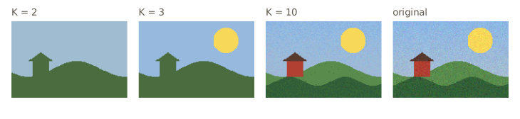
The trade-off is plain in the numbers: fewer colors, fewer bits, larger error. With \(K = 2\) the image costs about 4% of the raw size. Notice also that \(K = 10\) needed many more iterations: with more prototypes there are more ways to shuffle points between neighboring clusters, and each shuffle changes \(J\) only a little.
In practice. Real image compressors do much better than this, because neighboring pixels are strongly correlated. Quantizing small blocks of pixels, say 4 by 4, as single vectors captures some of that correlation; transform codes such as JPEG go further. Our goal here is only to see K-means in action.
Mixtures of Gaussians
A latent variable for the component
A Gaussian mixture in \(D\) dimensions has the density
\[p(\mathbf{x}) = \sum_{k=1}^{K} \pi_k \, \mathcal{N}(\mathbf{x} \mid \boldsymbol{\mu}_k, \boldsymbol{\Sigma}_k),\]with mixing coefficients \(\pi_k\) that satisfy \(0 \le \pi_k \le 1\) and \(\sum_k \pi_k = 1\). We now read this formula as the result of a two-stage random process.
Introduce a \(K\)-dimensional binary variable \(\mathbf{z}\) in 1-of-K coding: \(z_k \in \{0, 1\}\) and \(\sum_k z_k = 1\). It says which component produces \(\mathbf{x}\). Give it the distribution \(p(z_k = 1) = \pi_k\), and let \(\mathbf{x}\) be Gaussian given the component. Because exactly one \(z_k\) is 1, both distributions can be written as products with \(z_k\) in the exponent, which picks out the single active factor:
\[p(\mathbf{z}) = \prod_{k=1}^{K} \pi_k^{z_k}, \qquad p(\mathbf{x} \mid \mathbf{z}) = \prod_{k=1}^{K} \mathcal{N}(\mathbf{x} \mid \boldsymbol{\mu}_k, \boldsymbol{\Sigma}_k)^{z_k}.\]The joint distribution is \(p(\mathbf{x}, \mathbf{z}) = p(\mathbf{z}) \, p(\mathbf{x} \mid \mathbf{z})\). Summing it over the \(K\) possible values of \(\mathbf{z}\) gives back the mixture:
\[p(\mathbf{x}) = \sum_{\mathbf{z}} p(\mathbf{z}) \, p(\mathbf{x} \mid \mathbf{z}) = \sum_{k=1}^{K} \pi_k \, \mathcal{N}(\mathbf{x} \mid \boldsymbol{\mu}_k, \boldsymbol{\Sigma}_k).\]A variable like \(\mathbf{z}\), which is part of the model but never observed, is called a latent variable (or hidden variable). In the language of module 08, the model is the two-node directed graph \(\mathbf{z} \to \mathbf{x}\). With a data set, every observation \(\mathbf{x}_n\) gets its own latent \(\mathbf{z}_n\).
We have not changed the model: the density of \(\mathbf{x}\) is exactly what it was. What we have gained is a joint distribution \(p(\mathbf{x}, \mathbf{z})\) that is much simpler to work with than the marginal \(p(\mathbf{x})\), and that simplicity is what EM exploits.
Responsibilities
Once we see \(\mathbf{x}\), what do we believe about \(\mathbf{z}\)? Bayes’ theorem gives the posterior probability of component \(k\):
\[\begin{aligned} \gamma(z_k) \equiv p(z_k = 1 \mid \mathbf{x}) &= \frac{p(z_k = 1) \, p(\mathbf{x} \mid z_k = 1)}{\sum_{j=1}^{K} p(z_j = 1) \, p(\mathbf{x} \mid z_j = 1)} \\ &= \frac{\pi_k \, \mathcal{N}(\mathbf{x} \mid \boldsymbol{\mu}_k, \boldsymbol{\Sigma}_k)}{\sum_{j=1}^{K} \pi_j \, \mathcal{N}(\mathbf{x} \mid \boldsymbol{\mu}_j, \boldsymbol{\Sigma}_j)}. \end{aligned}\]Here \(\pi_k\) is the prior probability of component \(k\) and \(\gamma(z_k)\) its posterior probability after seeing \(\mathbf{x}\). We call \(\gamma(z_k)\) the responsibility that component \(k\) takes for explaining \(\mathbf{x}\). For data point \(n\) we write \(\gamma(z_{nk})\). Responsibilities are the soft version of the K-means indicators \(r_{nk}\): nonnegative and summing to one over \(k\), but not forced to be 0 or 1.
To compute them safely we work with logarithms. Densities in many dimensions, or far from every component, can be smaller than the smallest positive floating-point number, and then the ratio above becomes \(0/0\). Instead we compute \(a_{nk} = \ln \pi_k + \ln \mathcal{N}(\mathbf{x}_n \mid \boldsymbol{\mu}_k, \boldsymbol{\Sigma}_k)\) and use the log-sum-exp trick for the denominator: \(\ln \sum_k e^{a_{nk}} = a^\ast + \ln \sum_k e^{a_{nk} - a^\ast}\) with \(a^\ast = \max_k a_{nk}\), so the largest exponent is exactly zero and nothing underflows. Then \(\ln \gamma(z_{nk}) = a_{nk} - \ln \sum_j e^{a_{nj}}\). The Gaussian log-density itself comes from a Cholesky factor \(\boldsymbol{\Sigma} = \mathbf{L} \mathbf{L}^{\mathrm{T}}\): the log-determinant is \(2 \sum_i \ln L_{ii}\), and the quadratic form is \(\lVert \mathbf{y} \rVert^2\) with \(\mathbf{y}\) the solution of the triangular system \(\mathbf{L} \mathbf{y} = \mathbf{x} - \boldsymbol{\mu}\).
def log_gauss(X, mu, Sigma):
    """ln N(x_n | mu, Sigma) for every row of X, via a Cholesky factor Sigma = L L^T."""
    D = X.shape[1]
    L = np.linalg.cholesky(Sigma)
    y = solve_triangular(L, (X - mu).T, lower=True)   # y^T y = (x-mu)^T Sigma^-1 (x-mu)
    log_det = 2 * np.log(np.diag(L)).sum()
    return -0.5 * (D * np.log(2 * np.pi) + log_det + (y ** 2).sum(axis=0))

def gmm_log_joint(X, pi, mu, Sigma):
    """(N, K) matrix with entries ln pi_k + ln N(x_n | mu_k, Sigma_k)."""
    return np.column_stack([np.log(pi[k]) + log_gauss(X, mu[k], Sigma[k])
                            for k in range(len(pi))])

def gmm_e_step(X, pi, mu, Sigma):
    """Responsibilities gamma (N, K) and the log-likelihood ln p(X), in log space."""
    a = gmm_log_joint(X, pi, mu, Sigma)
    log_px = logsumexp(a, axis=1)                             # ln p(x_n) for every n
    return np.exp(a - log_px[:, None]), log_px.sum()

def gmm_loglik(X, pi, mu, Sigma):
    return gmm_e_step(X, pi, mu, Sigma)[1]

# check the log-density against SciPy
S_test = np.array([[1.0, 0.6], [0.6, 2.0]])
ours = log_gauss(X[:5], np.array([0.1, -0.2]), S_test)
ref = multivariate_normal(mean=[0.1, -0.2], cov=S_test).logpdf(X[:5])
print(f"largest difference from scipy.stats: {np.abs(ours - ref).max():.1e}")

# a point far from two 1-D components: the direct formula underflows, logs do not
x_far = np.array([[40.0]])
pi_2, mu_2 = np.array([0.5, 0.5]), np.array([[0.0], [1.0]])
S_2 = np.array([[[1.0]], [[1.0]]])
dens = pi_2 * np.exp([log_gauss(x_far, mu_2[k], S_2[k])[0] for k in range(2)])
with np.errstate(invalid="ignore"):
    print("direct responsibilities:", dens / dens.sum())
g_far = gmm_e_step(x_far, pi_2, mu_2, S_2)[0][0]
print(f"log-space responsibilities: {g_far[0]:.1e} and {g_far[1]:.6f}")
largest difference from scipy.stats: 8.9e-16
direct responsibilities: [nan nan]
log-space responsibilities: 7.0e-18 and 1.000000
The point at \(x = 40\) is 40 and 39 standard deviations from the two components. Both densities underflow to zero and the direct formula gives nan. In log space the answer is sensible: the exponents differ by \((40^2 - 39^2)/2 = 39.5\), so the nearer component is responsible with probability \(1 - e^{-39.5}\).
Sampling from the mixture
The latent-variable form tells us how to draw samples: first draw the component, then draw the point from that component. This is ancestral sampling (module 08): sample each variable after its parents. A sample of pairs \((\mathbf{x}_n, \mathbf{z}_n)\) is called complete data; if we throw away the \(\mathbf{z}_n\) and keep only the \(\mathbf{x}_n\), we have incomplete data, which is what we observe in practice.
We draw 500 points from a three-component mixture of our choosing and then ask how well the responsibilities, computed with the true parameters, recover the hidden labels.
def sample_gmm(n, pi, mu, Sigma, rng):
    """Ancestral sampling: draw z_n from pi, then x_n from component z_n."""
    z = rng.choice(len(pi), size=n, p=pi)
    X = np.empty((n, mu.shape[1]))
    for k in range(len(pi)):
        X[z == k] = rng.multivariate_normal(mu[k], Sigma[k], size=np.sum(z == k))
    return X, z

pi3 = np.array([0.45, 0.35, 0.20])
mu3 = np.array([[0.0, 0.0], [3.0, 1.0], [1.0, 3.0]])
Sigma3 = np.array([[[1.0, 0.5], [0.5, 1.0]],
                   [[0.6, 0.0], [0.0, 1.5]],
                   [[1.2, -0.6], [-0.6, 0.8]]])
X3, z3 = sample_gmm(500, pi3, mu3, Sigma3, np.random.default_rng(5))
gamma3, _ = gmm_e_step(X3, pi3, mu3, Sigma3)
print("points per component:", np.bincount(z3))
print("responsibilities of the first three points:\n", gamma3[:3])
print("their true components:", z3[:3])
hit = np.mean(gamma3.argmax(axis=1) == z3)
print(f"most responsible component = true component for {hit:.1%} of points")
print("points with no responsibility above 0.9:", np.sum(gamma3.max(axis=1) < 0.9))
points per component: [237 162 101]
responsibilities of the first three points:
 [[0.0729 0.8939 0.0332]
 [0.0531 0.2058 0.7411]
 [0.0077 0.9132 0.0791]]
their true components: [2 2 1]
most responsible component = true component for 88.8% of points
points with no responsibility above 0.9: 147
Even with the true parameters, the labels cannot all be recovered. Counting components from 0, as the code does, the very first point came from component 2 but lies where component 1 is far more likely, so the responsibilities favor component 1. The components overlap, and a point in the overlap could have come from either. The responsibilities record that doubt by spreading the probability across components, where a hard assignment would hide it.
Maximum likelihood
Now suppose we observe \(\mathbf{x}_1, \dots, \mathbf{x}_N\), independently drawn from a mixture with unknown parameters. We stack the observations as the rows of an \(N \times D\) matrix \(\mathbf{X}\), and the latent variables as the rows of an \(N \times K\) matrix \(\mathbf{Z}\). The log-likelihood is
\[\ln p(\mathbf{X} \mid \boldsymbol{\pi}, \boldsymbol{\mu}, \boldsymbol{\Sigma}) = \sum_{n=1}^{N} \ln \left\{ \sum_{k=1}^{K} \pi_k \, \mathcal{N}(\mathbf{x}_n \mid \boldsymbol{\mu}_k, \boldsymbol{\Sigma}_k) \right\}.\]Compare it with a single Gaussian, where the log sits directly on the Gaussian, cancels the exponential, and leaves a quadratic in \(\boldsymbol{\mu}\) with a closed-form maximum. Here a sum sits inside the log, and setting the derivatives to zero does not give a closed form. Before we find a way around that, two features of this likelihood need attention.
Singularities
Take a mixture in which one component, say component \(j\), has covariance \(\sigma_j^2 \mathbf{I}\), and place its mean exactly on a data point, \(\boldsymbol{\mu}_j = \mathbf{x}_n\). That point then contributes the term
\[\mathcal{N}(\mathbf{x}_n \mid \mathbf{x}_n, \sigma_j^2 \mathbf{I}) = \frac{1}{(2 \pi \sigma_j^2)^{D/2}}\]to its mixture density, which grows without limit as \(\sigma_j \to 0\). The other points do not suffer, because another component with an ordinary covariance still gives each of them a reasonable density. So the log-likelihood goes to \(+\infty\): the maximum likelihood problem for a Gaussian mixture has no maximum at all, only these singularities where a component collapses onto a single point.
A single Gaussian cannot do this. If it shrinks onto one point, every other point gets a density that goes to zero exponentially fast, and the product goes to zero, not infinity. The trouble needs at least two components: one that covers the data and one that is free to collapse.
S_all = np.cov(X.T, bias=True)                  # ML covariance of the whole data set
nearest = np.sqrt((sq_dists(X, X) + np.diag(np.full(N, np.inf))).min(axis=1))
n0 = nearest.argmax()                           # the most isolated data point
print(f"component 2 sits on x_{n0}; its nearest neighbor is {nearest[n0]:.2f} away")
print("   sigma   mixture ln p   single Gaussian ln p")
for sigma in [1e-1, 1e-2, 1e-4, 1e-8, 1e-16]:
    S_small = sigma ** 2 * np.eye(D)
    mix = gmm_loglik(X, np.array([0.5, 0.5]), np.array([X.mean(axis=0), X[n0]]),
                     np.array([S_all, S_small]))
    single = log_gauss(X, X[n0], S_small).sum()
    print(f"{sigma:8.0e} {mix:14.2f} {single:22.3e}")
component 2 sits on x_22; its nearest neighbor is 0.51 away
   sigma   mixture ln p   single Gaussian ln p
   1e-01        -811.30             -4.228e+04
   1e-02        -806.69             -4.309e+06
   1e-04        -797.48             -4.311e+10
   1e-08        -779.06             -4.311e+18
   1e-16        -742.22             -4.311e+34
Component 1 is the Gaussian fitted to the whole data set; component 2 sits on the most isolated data point, so that no other point shares its spike, and shrinks. Each tenfold decrease in \(\sigma\) adds \(D \ln 10 \approx 4.6\) to the mixture log-likelihood. The climb is slow, only logarithmic, but it never stops. Meanwhile a single Gaussian collapsing on the same point heads to \(-\infty\).
Watch out. These singularities are a form of severe overfitting, and gradient methods or EM can fall into them, especially with small data sets, many components, or isolated points. We will see EM do exactly that below. The usual remedies are to detect a collapsing component (a covariance whose determinant or smallest eigenvalue becomes tiny) and restart it with a new mean and a broad covariance, or to add a prior that keeps variances away from zero (the MAP version of EM, below). The Bayesian treatment of mixtures in module 10 does not have this problem.
Identifiability
The second feature is harmless for density estimation but matters for interpretation. If we swap the labels of two components, exchanging their \((\pi_k, \boldsymbol{\mu}_k, \boldsymbol{\Sigma}_k)\), the density does not change. So every setting of the parameters with distinct components has \(K!\) equivalent settings, one per ordering, all with the same likelihood. A model whose parameters cannot be recovered uniquely from the distribution they define is said to be not identifiable.
for perm in permutations(range(3)):
    p = list(perm)
    ll = gmm_loglik(X3, pi3[p], mu3[p], Sigma3[p])
    print("component order", perm, f" ln p = {ll:.6f}")
component order (0, 1, 2)  ln p = -1731.952176
component order (0, 2, 1)  ln p = -1731.952176
component order (1, 0, 2)  ln p = -1731.952176
component order (1, 2, 0)  ln p = -1731.952176
component order (2, 0, 1)  ln p = -1731.952176
component order (2, 1, 0)  ln p = -1731.952176
For a density model, any of the \(K!\) labelings is as good as any other. It becomes an issue when we want to say “component 1 means short eruptions”: a different run may call it component 2. We handle this by matching components after fitting, as we will do below.
EM for Gaussian mixtures
Equating the gradient of the log-likelihood to zero does not solve the problem, but it does tell us what a solution must satisfy, and that turns out to suggest an algorithm.
The means. The derivative of a Gaussian density with respect to its mean is \(\partial \mathcal{N}(\mathbf{x} \mid \boldsymbol{\mu}, \boldsymbol{\Sigma}) / \partial \boldsymbol{\mu} = \mathcal{N}(\mathbf{x} \mid \boldsymbol{\mu}, \boldsymbol{\Sigma}) \, \boldsymbol{\Sigma}^{-1} (\mathbf{x} - \boldsymbol{\mu})\). Differentiating the log-likelihood with respect to \(\boldsymbol{\mu}_k\), the chain rule through the log gives
\[\begin{aligned} \frac{\partial \ln p(\mathbf{X})}{\partial \boldsymbol{\mu}_k} &= \sum_{n=1}^{N} \frac{\pi_k \, \mathcal{N}(\mathbf{x}_n \mid \boldsymbol{\mu}_k, \boldsymbol{\Sigma}_k)}{\sum_j \pi_j \, \mathcal{N}(\mathbf{x}_n \mid \boldsymbol{\mu}_j, \boldsymbol{\Sigma}_j)} \, \boldsymbol{\Sigma}_k^{-1} (\mathbf{x}_n - \boldsymbol{\mu}_k) \\ &= \sum_{n=1}^{N} \gamma(z_{nk}) \, \boldsymbol{\Sigma}_k^{-1} (\mathbf{x}_n - \boldsymbol{\mu}_k). \end{aligned}\]The responsibilities appear by themselves. Set this to zero and multiply on the left by \(\boldsymbol{\Sigma}_k\) (assumed invertible):
\[\boldsymbol{\mu}_k = \frac{1}{N_k} \sum_{n=1}^{N} \gamma(z_{nk}) \, \mathbf{x}_n, \qquad N_k = \sum_{n=1}^{N} \gamma(z_{nk}).\]Here \(N_k\) is the effective number of points assigned to component \(k\), and the mean is a weighted average of all the data, each point weighted by how responsible component \(k\) is for it. With hard 0/1 responsibilities this is exactly the K-means M step.
The covariances. It is easiest to differentiate with respect to the precision \(\boldsymbol{\Lambda}_k = \boldsymbol{\Sigma}_k^{-1}\), using \(\partial \ln \lvert \boldsymbol{\Lambda} \rvert / \partial \boldsymbol{\Lambda} = \boldsymbol{\Lambda}^{-1}\) and \(\partial (\mathbf{a}^{\mathrm{T}} \boldsymbol{\Lambda} \mathbf{a}) / \partial \boldsymbol{\Lambda} = \mathbf{a} \mathbf{a}^{\mathrm{T}}\) (Bishop’s Appendix C). The log of a Gaussian is \(\tfrac{1}{2} \ln \lvert \boldsymbol{\Lambda} \rvert - \tfrac{1}{2} (\mathbf{x} - \boldsymbol{\mu})^{\mathrm{T}} \boldsymbol{\Lambda} (\mathbf{x} - \boldsymbol{\mu})\) plus a constant, so the same chain-rule step as before gives
\[\frac{\partial \ln p(\mathbf{X})}{\partial \boldsymbol{\Lambda}_k} = \frac{1}{2} \sum_{n=1}^{N} \gamma(z_{nk}) \left\{ \boldsymbol{\Sigma}_k - (\mathbf{x}_n - \boldsymbol{\mu}_k)(\mathbf{x}_n - \boldsymbol{\mu}_k)^{\mathrm{T}} \right\} = \mathbf{0}\]and solving for \(\boldsymbol{\Sigma}_k\),
\[\boldsymbol{\Sigma}_k = \frac{1}{N_k} \sum_{n=1}^{N} \gamma(z_{nk}) (\mathbf{x}_n - \boldsymbol{\mu}_k)(\mathbf{x}_n - \boldsymbol{\mu}_k)^{\mathrm{T}}.\]This is the maximum likelihood covariance of a single Gaussian from module 02, with each point weighted by its responsibility and the count replaced by \(N_k\).
The mixing coefficients. These must sum to one, so we maximize \(\ln p(\mathbf{X}) + \lambda \left( \sum_k \pi_k - 1 \right)\) with a Lagrange multiplier \(\lambda\) (Appendix E). The derivative with respect to \(\pi_k\) is
\[\sum_{n=1}^{N} \frac{\mathcal{N}(\mathbf{x}_n \mid \boldsymbol{\mu}_k, \boldsymbol{\Sigma}_k)}{\sum_j \pi_j \, \mathcal{N}(\mathbf{x}_n \mid \boldsymbol{\mu}_j, \boldsymbol{\Sigma}_j)} + \lambda = 0.\]Multiply by \(\pi_k\): the sum becomes \(\sum_n \gamma(z_{nk}) = N_k\), so \(N_k + \lambda \pi_k = 0\). Summing over \(k\) and using \(\sum_k N_k = N\) and \(\sum_k \pi_k = 1\) gives \(\lambda = -N\), and therefore
\[\pi_k = \frac{N_k}{N}.\]Each mixing coefficient is the average responsibility of its component. It is automatically between 0 and 1, so the inequality constraints take care of themselves.
These three equations are not a solution, because the responsibilities on the right depend on the parameters on the left. But they suggest an iteration: compute the responsibilities from the current parameters, then treat them as fixed and apply the three formulas. That iteration is EM for Gaussian mixtures.
Result. EM for a Gaussian mixture. Initialize \(\pi_k\), \(\boldsymbol{\mu}_k\), \(\boldsymbol{\Sigma}_k\), then repeat until the log-likelihood (or the parameters) stops changing.
E step: compute \(\gamma(z_{nk}) \propto \pi_k \, \mathcal{N}(\mathbf{x}_n \mid \boldsymbol{\mu}_k, \boldsymbol{\Sigma}_k)\), normalized over \(k\), with the current parameters.
M step: with \(N_k = \sum_n \gamma(z_{nk})\), set \(\boldsymbol{\mu}_k^{\mathrm{new}} = \frac{1}{N_k} \sum_n \gamma(z_{nk}) \mathbf{x}_n\), then \(\boldsymbol{\Sigma}_k^{\mathrm{new}} = \frac{1}{N_k} \sum_n \gamma(z_{nk}) (\mathbf{x}_n - \boldsymbol{\mu}_k^{\mathrm{new}})(\mathbf{x}_n - \boldsymbol{\mu}_k^{\mathrm{new}})^{\mathrm{T}}\) (using the new means), and \(\pi_k^{\mathrm{new}} = N_k / N\).
Each E step followed by an M step never decreases \(\ln p(\mathbf{X} \mid \boldsymbol{\pi}, \boldsymbol{\mu}, \boldsymbol{\Sigma})\); we prove this in the last part of the module.
In code, the E step is gmm_e_step from above, which also returns the log-likelihood at the current parameters, and the M step is a few lines.
def gmm_m_step(X, gamma):
    """Re-estimate pi, mu, Sigma from the responsibilities gamma (N, K)."""
    N_k = gamma.sum(axis=0)  # effective number of points per component
    mu = gamma.T @ X / N_k[:, None]
    Sigma = np.empty((len(N_k), X.shape[1], X.shape[1]))
    for k in range(len(N_k)):
        diff = X - mu[k]                              # deviations from the NEW mean
        Sigma[k] = (gamma[:, k, None] * diff).T @ diff / N_k[k]
    return N_k / len(X), mu, Sigma

def gmm_em(X, pi, mu, Sigma, max_iter=500, tol=1e-8):
    """EM for a Gaussian mixture.
    Returns (pi, mu, Sigma), the last responsibilities, and ln p for every iteration."""
    loglik = []
    for it in range(max_iter):
        gamma, ll = gmm_e_step(X, pi, mu, Sigma)  # E step; ll = ln p(X), current theta
        loglik.append(ll)
        if it > 0 and loglik[-1] - loglik[-2] < tol:
            break
        pi, mu, Sigma = gmm_m_step(X, gamma)         # M step
    return (pi, mu, Sigma), gamma, loglik
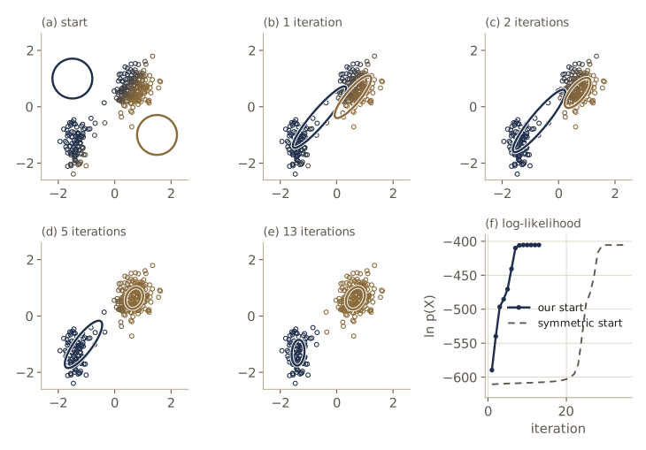
We fit two components to the geyser-like data, starting from the same poor means we gave K-means, with equal mixing coefficients and covariances \(0.5 \mathbf{I}\).
pi0 = np.array([0.5, 0.5])
Sigma0 = np.array([0.5 * np.eye(D), 0.5 * np.eye(D)])
(pi_em, mu_em, Sigma_em), gamma_em, ll_em = gmm_em(X, pi0, mu_init, Sigma0)
for it in [0, 1, 2, 3, 5, 8, len(ll_em) - 1]:
    print(f"iteration {it:2d}: ln p(X) = {ll_em[it]:10.3f}")
print("ln p never decreases:", bool(np.all(np.diff(ll_em) >= -1e-9)))

scale, shift = X_raw.std(axis=0), X_raw.mean(axis=0)      # back to minutes
for k in np.argsort(mu_em[:, 0]):
    m = mu_em[k] * scale + shift
    S = Sigma_em[k] * np.outer(scale, scale)
    corr = S[0, 1] / np.sqrt(S[0, 0] * S[1, 1])
    sd = np.sqrt(np.diag(S))
    print(f"pi = {pi_em[k]:.3f}  mean = ({m[0]:.2f}, {m[1]:.1f})  "
          f"sd = ({sd[0]:.2f}, {sd[1]:.1f})  correlation = {corr:.2f}")
iteration  0: ln p(X) =  -1703.616
iteration  1: ln p(X) =   -589.614
iteration  2: ln p(X) =   -539.834
iteration  3: ln p(X) =   -496.666
iteration  5: ln p(X) =   -470.536
iteration  8: ln p(X) =   -406.045
iteration 13: ln p(X) =   -405.477
ln p never decreases: True
pi = 0.327  mean = (1.99, 54.5)  sd = (0.26, 6.2)  correlation = 0.13
pi = 0.673  mean = (4.30, 80.5)  sd = (0.38, 5.4)  correlation = 0.28
The log-likelihood rises at every iteration, fast at first and then more slowly, and it has converged to our tolerance after 13 iterations. Translated back to minutes, the fit is close to the Gaussians we generated from: a short cluster with 33% of the points centered at (1.99, 54.5), against the true (2.0, 54.5), and a long cluster at (4.30, 80.5), against (4.3, 80.0). The fitted standard deviations 0.26, 6.2, 0.38, and 5.4 compare with the true 0.26, 5.8, 0.41, and 6.0, and the fitted correlations are somewhat weaker than the true 0.23 and 0.38. With about 100 and 200 points per cluster, estimates of this quality are what we should expect.
Two checks confirm that EM reached a stationary point and show how to reach it faster. At a maximum, the gradient of the log-likelihood with respect to the means must vanish; we check with central differences. Then we start EM from the K-means solution, with each covariance set to the sample covariance of its K-means cluster and each mixing coefficient to its cluster’s fraction of the points. This is the most common way to initialize EM in practice.
def num_grad_mu(X, pi, mu, Sigma, h=1e-6):
    """Central-difference gradient of ln p(X) with respect to the means."""
    g = np.zeros_like(mu)
    for idx in np.ndindex(mu.shape):
        e = np.zeros_like(mu)
        e[idx] = h
        up, down = gmm_loglik(X, pi, mu + e, Sigma), gmm_loglik(X, pi, mu - e, Sigma)
        g[idx] = (up - down) / (2 * h)
    return g

grad = num_grad_mu(X, pi_em, mu_em, Sigma_em)
print(f"largest gradient entry at the EM solution: {np.abs(grad).max():.1e}")

pi_km = np.bincount(r_km) / N
Sigma_km = np.array([np.cov(X[r_km == k].T, bias=True) for k in range(2)])
_, _, ll_from_km = gmm_em(X, pi_km, mu_km, Sigma_km)
for name, ll in [("K-means start:", ll_from_km), ("poor start:", ll_em)]:
    print(f"from the {name:15s}{len(ll) - 1:2d} iterations, final ln p = {ll[-1]:.3f}")
largest gradient entry at the EM solution: 4.2e-05
from the K-means start:  5 iterations, final ln p = -405.477
from the poor start:    13 iterations, final ln p = -405.477
Both runs end at the same log-likelihood, and the K-means start needs fewer iterations. Each EM iteration also costs more than a K-means iteration (covariances, Cholesky factors, exponentials), which is another reason to let K-means do the rough work first.
The start matters in a second way. Suppose we place the two initial means symmetrically across the data’s long axis:
mu_sym = np.array([[-1.5, 1.5], [1.5, -1.5]])
_, _, ll_sym = gmm_em(X, pi0, mu_sym, Sigma0)
checkpoints = [1, 5, 10, 20, 25, 30]
print("ln p at iterations", checkpoints, np.round(np.array(ll_sym)[checkpoints], 1))
print(f"converged after {len(ll_sym) - 1} iterations at ln p = {ll_sym[-1]:.3f}")
ll_single = log_gauss(X, X.mean(axis=0), S_all).sum()
print(f"a single Gaussian fitted to all the data: ln p = {ll_single:.3f}")
ln p at iterations [1, 5, 10, 20, 25, 30] [-610.6 -609.4 -608.4 -603.  -491.9 -405.5]
converged after 35 iterations at ln p = -405.477
a single Gaussian fitted to all the data: ln p = -611.234
For about twenty iterations the log-likelihood barely moves, stuck near the value of a single Gaussian: both components sit on top of each other and cover all the data, a nearly stationary configuration. The symmetry breaks slowly, and then EM finds the two clusters within about ten more iterations. A tiny change in \(\ln p\) per iteration does not always mean convergence, which is why practical code combines a tolerance with a generous iteration limit, or several starts.
Watching a component collapse
Now the singularity in practice. We take 20 points from a standard normal plus one outlier at \(x = 6\), and start a two-component mixture in one dimension with one component centered on the outlier.
col_rng = np.random.default_rng(4)
x_col = np.concatenate([col_rng.standard_normal(20), [6.0]])[:, None]  # outlier last
pi_c, mu_c = np.array([0.5, 0.5]), np.array([[0.0], [6.0]])
Sigma_c = np.array([[[1.0]], [[0.5]]])
for it in range(4):
    try:
        gamma_c, ll_c = gmm_e_step(x_col, pi_c, mu_c, Sigma_c)
    except np.linalg.LinAlgError as err:
        print(f"iteration {it}: the E step fails ({err})")
        break
    var2 = Sigma_c[1, 0, 0]
    print(f"iteration {it}: variance of component 2 = {var2:.2e}, ln p = {ll_c:.2f}")
    pi_c, mu_c, Sigma_c = gmm_m_step(x_col, gamma_c)
iteration 0: variance of component 2 = 5.00e-01, ln p = -46.20
iteration 1: variance of component 2 = 2.01e-04, ln p = -31.44
iteration 2: the E step fails (Matrix is not positive definite)
After one E step the second component is responsible for the outlier and for essentially nothing else. The M step sets its mean on the outlier and its variance to a weighted spread that is almost zero; the log-likelihood jumps. One step later every other responsibility has underflowed to exactly zero, the variance is exactly zero, and the Cholesky factorization fails. This is the singularity of the previous section, reached by EM on its own. We return to this example with a fix when we meet MAP estimation with EM.
An alternative view of EM
The derivation above was specific to Gaussian mixtures. We now describe EM for any model with latent variables, in a way that shows where the “expectation” in the name comes from.
Let \(\mathbf{X}\) be all the observed data, \(\mathbf{Z}\) all the latent variables, and \(\boldsymbol{\theta}\) all the parameters. The log-likelihood is
\[\ln p(\mathbf{X} \mid \boldsymbol{\theta}) = \ln \left\{ \sum_{\mathbf{Z}} p(\mathbf{X}, \mathbf{Z} \mid \boldsymbol{\theta}) \right\},\]with an integral in place of the sum if \(\mathbf{Z}\) is continuous. The sum inside the logarithm is what makes it hard. Even when the joint distribution is a friendly member of the exponential family, the marginal usually is not.
Imagine instead that we were handed \(\mathbf{Z}\) as well. Then \(\{\mathbf{X}, \mathbf{Z}\}\) is the complete data set, \(\mathbf{X}\) alone is incomplete, and we could maximize the complete-data log-likelihood \(\ln p(\mathbf{X}, \mathbf{Z} \mid \boldsymbol{\theta})\), which we assume is easy. We are not handed \(\mathbf{Z}\). All we know about it, given the data and a current guess \(\boldsymbol{\theta}^{\mathrm{old}}\), is the posterior \(p(\mathbf{Z} \mid \mathbf{X}, \boldsymbol{\theta}^{\mathrm{old}})\). So we average the complete-data log-likelihood over that posterior:
\[\mathcal{Q}(\boldsymbol{\theta}, \boldsymbol{\theta}^{\mathrm{old}}) = \sum_{\mathbf{Z}} p(\mathbf{Z} \mid \mathbf{X}, \boldsymbol{\theta}^{\mathrm{old}}) \ln p(\mathbf{X}, \mathbf{Z} \mid \boldsymbol{\theta}).\]In \(\mathcal{Q}\) the log is applied to the joint distribution itself, not to a sum of joints, so maximizing it over \(\boldsymbol{\theta}\) is as easy as the complete-data problem.
Definition. The EM algorithm for a model \(p(\mathbf{X}, \mathbf{Z} \mid \boldsymbol{\theta})\): choose \(\boldsymbol{\theta}^{\mathrm{old}}\), then repeat two steps.
The E step, computing the posterior \(p(\mathbf{Z} \mid \mathbf{X}, \boldsymbol{\theta}^{\mathrm{old}})\) (in practice, the expectations that \(\mathcal{Q}\) needs).
The M step, setting \(\boldsymbol{\theta}^{\mathrm{new}} = \arg\max_{\boldsymbol{\theta}} \mathcal{Q}(\boldsymbol{\theta}, \boldsymbol{\theta}^{\mathrm{old}})\) and then \(\boldsymbol{\theta}^{\mathrm{old}} \leftarrow \boldsymbol{\theta}^{\mathrm{new}}\).
Stop when the log-likelihood or the parameters stop changing.
Why the expectation, rather than, say, plugging in the most probable \(\mathbf{Z}\)? The last part of the module answers this: with the expectation, every cycle provably increases \(\ln p(\mathbf{X} \mid \boldsymbol{\theta})\) unless it is already at a stationary point.
Two remarks before the examples. First, with a prior \(p(\boldsymbol{\theta})\) we can find a MAP estimate instead: the E step is unchanged and the M step maximizes \(\mathcal{Q}(\boldsymbol{\theta}, \boldsymbol{\theta}^{\mathrm{old}}) + \ln p(\boldsymbol{\theta})\); a suitable prior removes the singularities we just met. Second, the “latent” variables can simply be missing entries of the data. If some coordinates of some \(\mathbf{x}_n\) were not recorded, we treat them as latent and let EM average over them. This is valid when the values are missing at random: whether a value is missing must not depend on the value itself. A sensor that fails whenever its reading is very high violates this, and then the missing pattern carries information that EM would ignore. Module 12 uses EM with missing data for probabilistic PCA.
Gaussian mixtures revisited
For the Gaussian mixture, \(p(\mathbf{z}_n) = \prod_k \pi_k^{z_{nk}}\) and \(p(\mathbf{x}_n \mid \mathbf{z}_n) = \prod_k \mathcal{N}(\mathbf{x}_n \mid \boldsymbol{\mu}_k, \boldsymbol{\Sigma}_k)^{z_{nk}}\), so the complete-data likelihood and its logarithm are
\[p(\mathbf{X}, \mathbf{Z} \mid \boldsymbol{\mu}, \boldsymbol{\Sigma}, \boldsymbol{\pi}) = \prod_{n=1}^{N} \prod_{k=1}^{K} \pi_k^{z_{nk}} \mathcal{N}(\mathbf{x}_n \mid \boldsymbol{\mu}_k, \boldsymbol{\Sigma}_k)^{z_{nk}},\] \[\ln p(\mathbf{X}, \mathbf{Z} \mid \boldsymbol{\mu}, \boldsymbol{\Sigma}, \boldsymbol{\pi}) = \sum_{n=1}^{N} \sum_{k=1}^{K} z_{nk} \left\{ \ln \pi_k + \ln \mathcal{N}(\mathbf{x}_n \mid \boldsymbol{\mu}_k, \boldsymbol{\Sigma}_k) \right\}.\]Compared with the incomplete-data log-likelihood, the sum over \(k\) and the logarithm have traded places. The log now acts on each Gaussian directly, and the problem falls apart into \(K\) separate single-Gaussian fits: component \(k\)’s mean and covariance are the sample mean and covariance of the points with \(z_{nk} = 1\), and, with a Lagrange multiplier as before, \(\pi_k = \frac{1}{N} \sum_n z_{nk}\), the fraction of points in group \(k\).
We do not have \(\mathbf{Z}\), so we take the expectation. The posterior of \(\mathbf{Z}\) is proportional to the joint, \(\prod_n \prod_k [\pi_k \mathcal{N}(\mathbf{x}_n \mid \boldsymbol{\mu}_k, \boldsymbol{\Sigma}_k)]^{z_{nk}}\). It factorizes over \(n\), so the \(\mathbf{z}_n\) are independent given the data (d-separation in the graph of module 08 says the same). The expected value of the indicator \(z_{nk}\) is the posterior probability that it equals 1, which is the responsibility:
\[\mathbb{E}[z_{nk}] = \frac{\pi_k \, \mathcal{N}(\mathbf{x}_n \mid \boldsymbol{\mu}_k, \boldsymbol{\Sigma}_k)}{\sum_j \pi_j \, \mathcal{N}(\mathbf{x}_n \mid \boldsymbol{\mu}_j, \boldsymbol{\Sigma}_j)} = \gamma(z_{nk}).\]The complete-data log-likelihood is linear in the \(z_{nk}\), so its expectation replaces each \(z_{nk}\) by \(\gamma(z_{nk})\):
\[\mathcal{Q} = \mathbb{E}_{\mathbf{Z}}[\ln p(\mathbf{X}, \mathbf{Z} \mid \boldsymbol{\mu}, \boldsymbol{\Sigma}, \boldsymbol{\pi})] = \sum_{n=1}^{N} \sum_{k=1}^{K} \gamma(z_{nk}) \left\{ \ln \pi_k + \ln \mathcal{N}(\mathbf{x}_n \mid \boldsymbol{\mu}_k, \boldsymbol{\Sigma}_k) \right\}.\]Maximizing this with the responsibilities held fixed is the complete-data problem with fractional memberships, and it gives exactly the weighted means, weighted covariances, and \(\pi_k = N_k / N\) of the previous section. So the general recipe reproduces the algorithm we derived by hand.
We can check both halves of that statement numerically: the complete-data fit with the true labels, and the claim that gmm_m_step maximizes \(\mathcal{Q}\).
def fit_complete(X, z, K):
    """ML fit with observed labels: one Gaussian per group, pi = group fractions."""
    pi = np.array([np.mean(z == k) for k in range(K)])
    mu = np.array([X[z == k].mean(axis=0) for k in range(K)])
    Sigma = np.array([np.cov(X[z == k].T, bias=True) for k in range(K)])
    return pi, mu, Sigma

def gmm_Q(X, gamma, pi, mu, Sigma):
    """Expected complete-data log-likelihood for fixed responsibilities gamma."""
    return np.sum(gamma * gmm_log_joint(X, pi, mu, Sigma))

pi_cd, mu_cd, _ = fit_complete(X, z_true, 2)
order = np.argsort(mu_em[:, 0])                 # EM's components, short cluster first
print("complete data (labels):  pi =", pi_cd, " means:", mu_cd.ravel())
print("EM (no labels):          pi =", pi_em[order], " means:", mu_em[order].ravel())
agree = np.mean(order.argsort()[gamma_em.argmax(axis=1)] == z_true)
print(f"EM's top component matches the true label for {agree:.1%} of points")

gamma_old, _ = gmm_e_step(X, pi0, mu_init, Sigma0)  # responsibilities at the poor start
theta_new = gmm_m_step(X, gamma_old)
Q_best = gmm_Q(X, gamma_old, *theta_new)
q_rng = np.random.default_rng(11)
gaps = []
for _ in range(200):                                 # random nearby parameter settings
    pi_p = theta_new[0] * np.exp(0.1 * q_rng.standard_normal(2))
    A = np.eye(D) + 0.1 * q_rng.standard_normal((2, D, D))
    Sigma_p = A @ theta_new[2] @ np.transpose(A, (0, 2, 1))  # stays positive definite
    mu_p = theta_new[1] + 0.1 * q_rng.standard_normal((2, D))
    gaps.append(gmm_Q(X, gamma_old, pi_p / pi_p.sum(), mu_p, Sigma_p) - Q_best)
print(f"Q at the M-step parameters: {Q_best:.3f}")
print(f"the best of 200 perturbations is lower by {-max(gaps):.4f}")
complete data (labels):  pi = [0.3267 0.6733]  means: [-1.3676 -1.3023  0.6635  0.6318]
EM (no labels):          pi = [0.3267 0.6733]  means: [-1.3674 -1.3022  0.6635  0.6319]
EM's top component matches the true label for 100.0% of points
Q at the M-step parameters: -706.223
the best of 200 perturbations is lower by 10.2328
EM, which never saw the labels, lands within a few ten-thousandths of the fit that did see them, and its most responsible component agrees with the true label for every one of the 300 points. That is because these two clusters barely overlap; with overlapping clusters, the two fits would differ more. And none of the 200 random perturbations of the M-step parameters achieves a larger \(\mathcal{Q}\).
Relation to K-means
K-means makes hard assignments and EM soft ones, and otherwise the two look alike. In fact K-means is a limiting case of EM.
Take a mixture whose components all have the same covariance \(\epsilon \mathbf{I}\), with \(\epsilon\) a fixed constant rather than a parameter to learn. The responsibilities are
\[\gamma(z_{nk}) = \frac{\pi_k \exp\left\{ -\lVert \mathbf{x}_n - \boldsymbol{\mu}_k \rVert^2 / 2\epsilon \right\}}{\sum_j \pi_j \exp\left\{ -\lVert \mathbf{x}_n - \boldsymbol{\mu}_j \rVert^2 / 2\epsilon \right\}}.\]Let \(d_{nk} = \lVert \mathbf{x}_n - \boldsymbol{\mu}_k \rVert^2\) and let \(d_n^\ast\) be the smallest of them. Dividing the numerator and the denominator by \(\exp(-d_n^\ast / 2\epsilon)\) turns each exponent into \(-(d_{nk} - d_n^\ast)/2\epsilon\). For the nearest prototype the exponent is 0; for every other prototype it goes to \(-\infty\) as \(\epsilon \to 0\). So, as long as no \(\pi_k\) is zero and there are no ties, \(\gamma(z_{nk}) \to r_{nk}\), the K-means assignment. The M step for the means then becomes the K-means M step. (The \(\pi_k\) are still re-estimated as cluster fractions, but they no longer influence the assignments.)
The expected complete-data log-likelihood also turns into the distortion:
\[\mathcal{Q} = \sum_{n,k} \gamma(z_{nk}) \left\{ \ln \pi_k - \frac{D}{2} \ln(2 \pi \epsilon) - \frac{\lVert \mathbf{x}_n - \boldsymbol{\mu}_k \rVert^2}{2 \epsilon} \right\},\]and multiplying by \(\epsilon\) and letting \(\epsilon \to 0\),
\[\epsilon \, \mathcal{Q} \to -\frac{1}{2} \sum_{n,k} r_{nk} \lVert \mathbf{x}_n - \boldsymbol{\mu}_k \rVert^2 = -\frac{J}{2},\]because \(\epsilon \ln \epsilon \to 0\). Maximizing \(\mathcal{Q}\) becomes minimizing \(J\). We check both limits at the K-means solution, and then run EM with fixed small \(\epsilon\) from the same start as K-means.
pi_hard = np.bincount(r_km) / N
d2 = sq_dists(X, mu_km)
J_km = distortion(X, r_km, mu_km)
for eps in [1.0, 0.1, 0.01, 1e-3, 1e-6]:
    a = np.log(pi_hard) - D / 2 * np.log(2 * np.pi * eps) - d2 / (2 * eps)
    gamma_eps = np.exp(a - logsumexp(a, axis=1, keepdims=True))
    gap = np.abs(gamma_eps - np.eye(2)[r_km]).max()
    eps_Q = eps * np.sum(gamma_eps * a)
    print(f"eps = {eps:7.0e}: max |gamma - r| = {gap:.1e},  eps * Q = {eps_Q:9.3f}"
          f"   (-J/2 = {-J_km / 2:.3f})")

def em_isotropic(X, pi, mu, eps, max_iter=500):
    """EM for a mixture whose covariances are all fixed at eps * I; learns pi and mu."""
    for _ in range(max_iter):
        a = np.log(pi) - sq_dists(X, mu) / (2 * eps)
        gamma = np.exp(a - logsumexp(a, axis=1, keepdims=True))
        N_k = gamma.sum(axis=0)
        mu_new, pi = gamma.T @ X / N_k[:, None], N_k / len(X)
        if np.abs(mu_new - mu).max() < 1e-12:
            break
        mu = mu_new
    return mu_new

for eps in [1.0, 0.001]:
    diff = np.abs(em_isotropic(X, pi0, mu_init, eps) - mu_km).max()
    print(f"eps = {eps}: largest |mu_EM - mu_K-means| = {diff:.2e}")
eps =   1e+00: max |gamma - r| = 5.6e-01,  eps * Q =  -806.285   (-J/2 = -40.009)
eps =   1e-01: max |gamma - r| = 1.6e-02,  eps * Q =   -45.100   (-J/2 = -40.009)
eps =   1e-02: max |gamma - r| = 2.2e-21,  eps * Q =   -33.610   (-J/2 = -40.009)
eps =   1e-03: max |gamma - r| = 5.3e-210,  eps * Q =   -38.679   (-J/2 = -40.009)
eps =   1e-06: max |gamma - r| = 0.0e+00,  eps * Q =   -40.006   (-J/2 = -40.009)
eps = 1.0: largest |mu_EM - mu_K-means| = 6.53e-02
eps = 0.001: largest |mu_EM - mu_K-means| = 0.00e+00
At \(\epsilon = 1\) the responsibilities are far from hard, and EM’s means differ from the K-means prototypes. By \(\epsilon = 0.01\) the responsibilities are hard to within \(10^{-20}\). The scaled objective \(\epsilon \mathcal{Q}\) approaches \(-J/2\) more slowly, because the Gaussian’s normalizing constant contributes a term of order \(\epsilon \ln \epsilon\), but at \(\epsilon = 10^{-6}\) it agrees to two decimals. And EM with \(\epsilon = 0.001\) lands on the K-means prototypes exactly.
K-means estimates no covariances; it implicitly uses the same round covariance for every cluster, which is why it prefers compact, similar-sized clusters. A hard-assignment version that does estimate a full covariance per cluster is called elliptical K-means.
Mixtures of Bernoulli distributions
EM is not tied to Gaussians. Our next model is for binary data: vectors \(\mathbf{x} = (x_1, \dots, x_D)^{\mathrm{T}}\) with each \(x_i \in \{0, 1\}\), such as black-and-white images. The simplest model treats the \(D\) bits as independent Bernoulli variables with means \(\boldsymbol{\mu} = (\mu_1, \dots, \mu_D)^{\mathrm{T}}\):
\[p(\mathbf{x} \mid \boldsymbol{\mu}) = \prod_{i=1}^{D} \mu_i^{x_i} (1 - \mu_i)^{1 - x_i}.\]Its mean is \(\mathbb{E}[\mathbf{x}] = \boldsymbol{\mu}\) and its covariance is \(\operatorname{cov}[\mathbf{x}] = \operatorname{diag}\{\mu_i (1 - \mu_i)\}\), a diagonal matrix: this model cannot express that two pixels tend to be on together. A mixture can. For \(p(\mathbf{x} \mid \boldsymbol{\mu}, \boldsymbol{\pi}) = \sum_k \pi_k \, p(\mathbf{x} \mid \boldsymbol{\mu}_k)\), the mean is \(\sum_k \pi_k \boldsymbol{\mu}_k\), and since \(\mathbb{E}[\mathbf{x} \mathbf{x}^{\mathrm{T}}] = \sum_k \pi_k (\boldsymbol{\Sigma}_k + \boldsymbol{\mu}_k \boldsymbol{\mu}_k^{\mathrm{T}})\), where \(\boldsymbol{\Sigma}_k = \operatorname{diag}\{\mu_{ki}(1 - \mu_{ki})\}\) is the covariance of component \(k\), the covariance is
\[\operatorname{cov}[\mathbf{x}] = \sum_{k=1}^{K} \pi_k \left( \boldsymbol{\Sigma}_k + \boldsymbol{\mu}_k \boldsymbol{\mu}_k^{\mathrm{T}} \right) - \mathbb{E}[\mathbf{x}] \, \mathbb{E}[\mathbf{x}]^{\mathrm{T}},\]which is not diagonal in general. (The same formula holds for a mixture of any distributions with means \(\boldsymbol{\mu}_k\) and covariances \(\boldsymbol{\Sigma}_k\).) Here is a three-bit example: two components, one with the first two bits usually on and one with them usually off, and a third bit that is the same in both.
pi_b = np.array([0.5, 0.5])
mu_b = np.array([[0.9, 0.9, 0.2], [0.1, 0.1, 0.2]])
mean_mix = pi_b @ mu_b
second_moment = sum(pi_b[k] * (np.diag(mu_b[k] * (1 - mu_b[k]))      # Sigma_k
                               + np.outer(mu_b[k], mu_b[k]))
                    for k in range(2))
cov_mix = second_moment - np.outer(mean_mix, mean_mix)
b_rng = np.random.default_rng(8)
zb = b_rng.choice(2, size=200_000, p=pi_b)
xb = (b_rng.random((200_000, 3)) < mu_b[zb]).astype(float)    # ancestral sampling
print("covariance from the formula:\n", cov_mix)
print("sample covariance of 200,000 draws:\n", np.cov(xb.T, bias=True))
covariance from the formula:
 [[0.25 0.16 0.  ]
 [0.16 0.25 0.  ]
 [0.   0.   0.16]]
sample covariance of 200,000 draws:
 [[ 0.25    0.1596  0.0002]
 [ 0.1596  0.25   -0.0001]
 [ 0.0002 -0.0001  0.1597]]
The first two bits have covariance 0.16 even though they are independent within each component: knowing that bit 1 is on makes the first component more likely, and with it bit 2. The third bit, which behaves the same in both components, stays uncorrelated with the others.
EM for the Bernoulli mixture. The log-likelihood \(\ln p(\mathbf{X} \mid \boldsymbol{\mu}, \boldsymbol{\pi}) = \sum_n \ln \left\{ \sum_k \pi_k \, p(\mathbf{x}_n \mid \boldsymbol{\mu}_k) \right\}\) again has a sum inside the log. We introduce the same 1-of-K latent \(\mathbf{z}_n\), with \(p(\mathbf{z} \mid \boldsymbol{\pi}) = \prod_k \pi_k^{z_k}\) and \(p(\mathbf{x} \mid \mathbf{z}, \boldsymbol{\mu}) = \prod_k p(\mathbf{x} \mid \boldsymbol{\mu}_k)^{z_k}\). The complete-data log-likelihood is
\[\ln p(\mathbf{X}, \mathbf{Z} \mid \boldsymbol{\mu}, \boldsymbol{\pi}) = \sum_{n=1}^{N} \sum_{k=1}^{K} z_{nk} \left\{ \ln \pi_k + \sum_{i=1}^{D} \left[ x_{ni} \ln \mu_{ki} + (1 - x_{ni}) \ln (1 - \mu_{ki}) \right] \right\}.\]It is linear in the \(z_{nk}\), so \(\mathcal{Q}\) replaces them by responsibilities, which Bayes’ theorem gives as before: \(\gamma(z_{nk}) = \pi_k \, p(\mathbf{x}_n \mid \boldsymbol{\mu}_k) / \sum_j \pi_j \, p(\mathbf{x}_n \mid \boldsymbol{\mu}_j)\). That is the E step. For the M step, differentiate \(\mathcal{Q}\) with respect to \(\mu_{ki}\):
\[\sum_{n=1}^{N} \gamma(z_{nk}) \left\{ \frac{x_{ni}}{\mu_{ki}} - \frac{1 - x_{ni}}{1 - \mu_{ki}} \right\} = 0,\]which gives
\[\boldsymbol{\mu}_k = \bar{\mathbf{x}}_k \equiv \frac{1}{N_k} \sum_{n=1}^{N} \gamma(z_{nk}) \, \mathbf{x}_n, \qquad N_k = \sum_{n=1}^{N} \gamma(z_{nk}),\]the responsibility-weighted average of the binary vectors. (Multiply through by \(\mu_{ki}(1 - \mu_{ki})\) to see it.) The mixing coefficients come out as \(\pi_k = N_k / N\) by the same Lagrange argument as for Gaussians.
Note. Bernoulli mixtures have no singularities. Every \(p(\mathbf{x}_n \mid \boldsymbol{\mu}_k)\) is a probability, at most 1, so each term of the log-likelihood is at most \(\ln 1 = 0\) and the likelihood is bounded above. It can go to \(-\infty\) (a \(\mu_{ki}\) of exactly 0 or 1 that disagrees with some data point), but EM, which only moves uphill, will not go there from a sensible start.
We test the model on synthetic 8×8 binary images. We design four patterns, horizontal bars, vertical bars, a frame, and a pair of crossing diagonals, and generate each image by picking a pattern and then turning each pixel on with probability 0.7 where the pattern is on and 0.25 where it is off. That is heavy noise: a quarter of the background pixels are on.
def prototypes():
    """Four 8x8 patterns: horizontal bars, vertical bars, a frame, two diagonals."""
    P = np.zeros((4, 8, 8))
    P[0, [1, 2, 5, 6], :] = 1
    P[1, :, [1, 2, 5, 6]] = 1
    P[2, [0, 7], :] = 1
    P[2, :, [0, 7]] = 1
    P[3, np.arange(8), np.arange(8)] = 1
    P[3, np.arange(8), 7 - np.arange(8)] = 1
    return P.reshape(4, 64)

mu_true_b = np.where(prototypes() > 0, 0.7, 0.25)  # pixel on-probabilities, 4 patterns
pi_true_b = np.array([0.3, 0.25, 0.25, 0.2])
data_rng = np.random.default_rng(1)
z_b = data_rng.choice(4, size=600, p=pi_true_b)
X_b = (data_rng.random((600, 64)) < mu_true_b[z_b]).astype(float)
print("data:", X_b.shape, f"  fraction of pixels on: {X_b.mean():.3f}")
print("images per pattern:", np.bincount(z_b))
data: (600, 64)   fraction of pixels on: 0.446
images per pattern: [182 162 138 118]
The implementation mirrors the Gaussian one. The log of the component density is linear in \(\mathbf{x}\), so one matrix product computes it for all points and components at once. We clip \(\boldsymbol{\mu}\) slightly away from 0 and 1 so that the logarithms stay finite. The initial means are random numbers between 0.25 and 0.75.
def bernoulli_log_joint(X, pi, mu):
    """(N, K) matrix: ln pi_k + sum_i [x_ni ln mu_ki + (1 - x_ni) ln(1 - mu_ki)]."""
    mu = np.clip(mu, 1e-10, 1 - 1e-10)
    return np.log(pi) + X @ np.log(mu).T + (1 - X) @ np.log(1 - mu).T

def bernoulli_em(X, K, rng, max_iter=500, tol=1e-8):
    N, D = X.shape
    pi, mu = np.full(K, 1 / K), rng.uniform(0.25, 0.75, size=(K, D))
    loglik = []
    for it in range(max_iter):
        a = bernoulli_log_joint(X, pi, mu)                  # E step
        log_px = logsumexp(a, axis=1)
        gamma = np.exp(a - log_px[:, None])
        loglik.append(log_px.sum())
        if it > 0 and loglik[-1] - loglik[-2] < tol:
            break
        N_k = gamma.sum(axis=0)                             # M step
        mu, pi = gamma.T @ X / N_k[:, None], N_k / N
    return pi, mu, gamma, loglik

pi_hat_b, mu_hat_b, gamma_b, ll_b = bernoulli_em(X_b, 4, np.random.default_rng(0))
print(f"{len(ll_b) - 1} iterations; ln p at iterations 0, 1, 2, 5, and the last:")
print(np.round([ll_b[i] for i in [0, 1, 2, 5, len(ll_b) - 1]], 1))
print("ln p never decreases:", bool(np.all(np.diff(ll_b) >= -1e-9)))

def mismatch(p):
    return np.abs(mu_hat_b[list(p)] - mu_true_b).sum()
match = list(min(permutations(range(4)), key=mismatch))  # component of pattern j
pattern_of = np.argsort(match)  # pattern_of[k] = pattern learned by component k
print("mixing coefficients, pattern order:", pi_hat_b[match])
print("true mixing coefficients:          ", pi_true_b)
err = np.abs(mu_hat_b[match] - mu_true_b).mean()
print(f"mean |mu_hat - mu_true| per pixel: {err:.3f}")
right = np.mean(pattern_of[gamma_b.argmax(axis=1)] == z_b)
print(f"images assigned to their own pattern: {right:.1%}")
14 iterations; ln p at iterations 0, 1, 2, 5, and the last:
[-27754.  -24967.2 -23327.  -23007.4 -23007.4]
ln p never decreases: True
mixing coefficients, pattern order: [0.3037 0.2727 0.2302 0.1935]
true mixing coefficients:           [0.3  0.25 0.25 0.2 ]
mean |mu_hat - mu_true| per pixel: 0.026
images assigned to their own pattern: 99.3%
EM converges in 14 iterations, most of the gain coming in the first two. After matching components to patterns (the labels are arbitrary, as we saw under identifiability), the learned pixel probabilities are within a few hundredths of the true ones, and 99.3% of the images are assigned to the pattern that generated them. The mixing coefficients differ from the true ones by up to 0.02, and they are close to the fractions actually present in this sample (182, 162, 138, and 118 of 600 images, or 0.303, 0.270, 0.230, and 0.197), which is all the data can tell us. For comparison, a single multivariate Bernoulli fitted by maximum likelihood just averages all images pixel by pixel:
mu_single = X_b.mean(axis=0)
ll_single_b = bernoulli_log_joint(X_b, np.ones(1), mu_single[None, :]).sum()
print(f"single Bernoulli: ln p = {ll_single_b:.1f};  mixture of 4: {ll_b[-1]:.1f}")
lo, hi = mu_single.min(), mu_single.max()
print(f"single-model pixel probabilities lie in [{lo:.2f}, {hi:.2f}]")
single Bernoulli: ln p = -25846.5;  mixture of 4: -23007.4
single-model pixel probabilities lie in [0.33, 0.62]
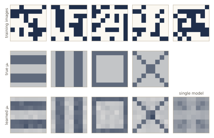
The single model’s pixel probabilities all sit in a narrow band around the overall fraction of pixels that are on: it cannot represent “these pixels come on together”, so it averages the four patterns into a blur, and its log-likelihood is far lower.
The Bernoulli mixture extends in two directions that we only mention. With a beta prior on each \(\mu_{ki}\) and a Dirichlet prior on \(\boldsymbol{\pi}\) (module 02), the MAP version of EM adds pseudo-counts to the M-step averages (exercise 8). And variables with more than two states are handled the same way with a mixture of products of categorical (multinomial) distributions. Bernoulli mixtures also prepare the ground for hidden Markov models over discrete variables in module 13.
EM for Bayesian linear regression
The latent variables in EM do not have to be discrete labels. In module 03 we chose the hyperparameters of Bayesian linear regression, the prior precision \(\alpha\) and the noise precision \(\beta\), by maximizing the evidence \(p(\mathbf{t} \mid \alpha, \beta) = \int p(\mathbf{t} \mid \mathbf{w}, \beta) \, p(\mathbf{w} \mid \alpha) \, \mathrm{d}\mathbf{w}\). The weights \(\mathbf{w}\) are integrated out, so we can treat them as latent variables and maximize the evidence with EM.
Recall the model: \(p(\mathbf{w} \mid \alpha) = \mathcal{N}(\mathbf{w} \mid \mathbf{0}, \alpha^{-1} \mathbf{I})\) with \(M\) weights, \(p(t_n \mid \mathbf{w}, \beta) = \mathcal{N}(t_n \mid \mathbf{w}^{\mathrm{T}} \boldsymbol{\phi}_n, \beta^{-1})\) with \(\boldsymbol{\phi}_n = \boldsymbol{\phi}(\mathbf{x}_n)\), and posterior \(p(\mathbf{w} \mid \mathbf{t}) = \mathcal{N}(\mathbf{w} \mid \mathbf{m}_N, \mathbf{S}_N)\) with \(\mathbf{S}_N^{-1} = \alpha \mathbf{I} + \beta \mathbf{\Phi}^{\mathrm{T}} \mathbf{\Phi}\) and \(\mathbf{m}_N = \beta \mathbf{S}_N \mathbf{\Phi}^{\mathrm{T}} \mathbf{t}\).
E step. Compute \(\mathbf{m}_N\) and \(\mathbf{S}_N\) with the current \(\alpha, \beta\). M step. The complete-data log-likelihood is
\[\ln p(\mathbf{t}, \mathbf{w} \mid \alpha, \beta) = \frac{M}{2} \ln \frac{\alpha}{2\pi} - \frac{\alpha}{2} \mathbf{w}^{\mathrm{T}} \mathbf{w} + \frac{N}{2} \ln \frac{\beta}{2\pi} - \frac{\beta}{2} \sum_{n=1}^{N} (t_n - \mathbf{w}^{\mathrm{T}} \boldsymbol{\phi}_n)^2.\]Its expectation under the posterior needs two moments. For a Gaussian, \(\mathbb{E}[\mathbf{w}^{\mathrm{T}} \mathbf{w}] = \mathbf{m}_N^{\mathrm{T}} \mathbf{m}_N + \operatorname{Tr}(\mathbf{S}_N)\), and \(\mathbb{E}[(t_n - \mathbf{w}^{\mathrm{T}} \boldsymbol{\phi}_n)^2] = (t_n - \mathbf{m}_N^{\mathrm{T}} \boldsymbol{\phi}_n)^2 + \boldsymbol{\phi}_n^{\mathrm{T}} \mathbf{S}_N \boldsymbol{\phi}_n\), whose sum over \(n\) is \(\lVert \mathbf{t} - \mathbf{\Phi} \mathbf{m}_N \rVert^2 + \operatorname{Tr}(\mathbf{\Phi}^{\mathrm{T}} \mathbf{\Phi} \mathbf{S}_N)\). Setting the derivatives with respect to \(\alpha\) and \(\beta\) to zero gives
\[\begin{aligned} \alpha^{\mathrm{new}} &= \frac{M}{\mathbf{m}_N^{\mathrm{T}} \mathbf{m}_N + \operatorname{Tr}(\mathbf{S}_N)}, \\ \frac{1}{\beta^{\mathrm{new}}} &= \frac{1}{N} \left\{ \lVert \mathbf{t} - \mathbf{\Phi} \mathbf{m}_N \rVert^2 + \operatorname{Tr}(\mathbf{\Phi}^{\mathrm{T}} \mathbf{\Phi} \mathbf{S}_N) \right\}. \end{aligned}\]The same fixed point as module 03. Module 03’s re-estimation used the effective number of parameters \(\gamma = \sum_i \lambda_i / (\alpha + \lambda_i)\), with \(\lambda_i\) the eigenvalues of \(\beta \mathbf{\Phi}^{\mathrm{T}} \mathbf{\Phi}\), and set \(\alpha = \gamma / \mathbf{m}_N^{\mathrm{T}} \mathbf{m}_N\) and \(1/\beta = \lVert \mathbf{t} - \mathbf{\Phi} \mathbf{m}_N \rVert^2 / (N - \gamma)\). The eigenvalues of \(\mathbf{S}_N\) are \(1/(\alpha + \lambda_i)\), so
\[\begin{aligned} \gamma &= \sum_i \frac{\lambda_i}{\alpha + \lambda_i} = M - \alpha \operatorname{Tr}(\mathbf{S}_N), \\ \beta \operatorname{Tr}(\mathbf{\Phi}^{\mathrm{T}} \mathbf{\Phi} \mathbf{S}_N) &= \operatorname{Tr}\left( (\mathbf{S}_N^{-1} - \alpha \mathbf{I}) \mathbf{S}_N \right) = \gamma. \end{aligned}\]At a fixed point of module 03’s iteration, \(\alpha \mathbf{m}_N^{\mathrm{T}} \mathbf{m}_N = \gamma = M - \alpha \operatorname{Tr}(\mathbf{S}_N)\), which rearranges to the EM update for \(\alpha\). Likewise \((N - \gamma)/\beta = \lVert \mathbf{t} - \mathbf{\Phi} \mathbf{m}_N \rVert^2\) is the same as \(N / \beta = \lVert \mathbf{t} - \mathbf{\Phi} \mathbf{m}_N \rVert^2 + \operatorname{Tr}(\mathbf{\Phi}^{\mathrm{T}} \mathbf{\Phi} \mathbf{S}_N)\), the EM update for \(\beta\). The two iterations differ along the way but share their fixed points. Each costs one \(M \times M\) factorization per step.
We test this on 30 noisy samples of \(\sin(2\pi x)\) with nine Gaussian basis functions plus a bias (\(M = 10\)), running both iterations from \(\alpha = \beta = 1\) until both hyperparameters change by less than one part in \(10^{10}\).
reg_rng = np.random.default_rng(3)
N_r = 30
x_r = reg_rng.uniform(0, 1, N_r)
t_r = np.sin(2 * np.pi * x_r) + 0.25 * reg_rng.standard_normal(N_r)
centers_r = np.linspace(0, 1, 9)

def design(x, s=0.1):
    """A bias column plus nine Gaussian basis functions of width s."""
    gauss = [np.exp(-(x - c) ** 2 / (2 * s ** 2)) for c in centers_r]
    return np.column_stack([np.ones_like(x)] + gauss)

Phi = design(x_r)
M = Phi.shape[1]
eig_PhiTPhi = np.linalg.eigvalsh(Phi.T @ Phi)

def posterior_w(alpha, beta):
    """m_N, S_N, and a Cholesky factor of S_N^{-1} = alpha I + beta Phi^T Phi."""
    A_chol = cho_factor(alpha * np.eye(M) + beta * Phi.T @ Phi)
    m_N = beta * cho_solve(A_chol, Phi.T @ t_r)
    S_N = cho_solve(A_chol, np.eye(M))           # we need S_N itself, for its trace
    return m_N, S_N, A_chol

def log_evidence(alpha, beta):
    m_N, _, A_chol = posterior_w(alpha, beta)
    E = beta / 2 * np.sum((t_r - Phi @ m_N) ** 2) + alpha / 2 * m_N @ m_N
    log_det_A = 2 * np.log(np.diag(A_chol[0])).sum()
    return (M / 2 * np.log(alpha) + N_r / 2 * np.log(beta) - E - log_det_A / 2
            - N_r / 2 * np.log(2 * np.pi))

def evidence_update(alpha, beta):
    """Module 03's re-estimation through gamma, the effective number of parameters."""
    m_N, _, _ = posterior_w(alpha, beta)
    lam = beta * eig_PhiTPhi
    g = np.sum(lam / (alpha + lam))
    return g / (m_N @ m_N), (N_r - g) / np.sum((t_r - Phi @ m_N) ** 2)

def em_update(alpha, beta):
    """E step: posterior over w. M step: maximize the expected complete-data log-lik."""
    m_N, S_N, _ = posterior_w(alpha, beta)
    alpha_new = M / (m_N @ m_N + np.trace(S_N))
    beta_new = N_r / (np.sum((t_r - Phi @ m_N) ** 2) + np.trace(Phi.T @ Phi @ S_N))
    return alpha_new, beta_new

def iterate(update, alpha=1.0, beta=1.0, tol=1e-10, max_iter=10_000):
    evidence = [log_evidence(alpha, beta)]
    for it in range(1, max_iter + 1):
        a, b = update(alpha, beta)
        evidence.append(log_evidence(a, b))
        done = abs(a - alpha) < tol * alpha and abs(b - beta) < tol * beta
        alpha, beta = a, b
        if done:
            break
    return alpha, beta, it, np.array(evidence)

for name, update in [("evidence re-estimation", evidence_update), ("EM", em_update)]:
    a, b, its, ev = iterate(update)
    print(f"{name}: {its} iterations, alpha = {a:.8f}, beta = {b:.8f}")
    print(f"    ln p(t) = {ev[-1]:.6f}; the evidence never drops: "
          f"{bool(np.all(np.diff(ev) > -1e-9))}")

m_N, S_N, _ = posterior_w(0.5, 20.0)  # the identities, at arbitrary alpha and beta
lam = 20.0 * eig_PhiTPhi
g = np.sum(lam / (0.5 + lam))
print(f"gamma = {g:.6f},  M - alpha Tr(S_N) = {M - 0.5 * np.trace(S_N):.6f},  "
      f"beta Tr(Phi^T Phi S_N) = {20.0 * np.trace(Phi.T @ Phi @ S_N):.6f}")
evidence re-estimation: 8 iterations, alpha = 3.76100886, beta = 15.52995270
    ln p(t) = -12.193308; the evidence never drops: True
EM: 22 iterations, alpha = 3.76100886, beta = 15.52995270
    ln p(t) = -12.193308; the evidence never drops: True
gamma = 8.496528,  M - alpha Tr(S_N) = 8.496528,  beta Tr(Phi^T Phi S_N) = 8.496528
Both iterations arrive at the same \(\alpha\) and \(\beta\) to eight significant digits and the same maximal evidence. EM takes about three times as many iterations here, but every one of its steps raised the evidence, a guarantee we are about to prove. The last line confirms the two trace identities.
The same idea applies to the relevance vector machine of module 07, which has a separate precision \(\alpha_i\) for each weight. Treating \(\mathbf{w}\) as latent, the M step gives \(\alpha_i^{\mathrm{new}} = 1 / (m_i^2 + \Sigma_{ii})\), with \(m_i\) and \(\Sigma_{ii}\) the posterior mean and variance of \(w_i\), and a \(\beta\) update of the same form as above. These have the same fixed points as the re-estimation equations derived there by differentiating the evidence directly (Bishop §9.3.4).
The EM algorithm in general
We have run EM on four models and watched the log-likelihood climb every time. Now we prove that it must, for any model, and in doing so we find a more flexible way to think about the algorithm.
A lower bound on the log-likelihood
As before, \(\mathbf{X}\) is observed, \(\mathbf{Z}\) is latent (take it discrete; for continuous \(\mathbf{Z}\) replace sums by integrals), and \(\boldsymbol{\theta}\) are the parameters. Let \(q(\mathbf{Z})\) be any probability distribution over the latent variables. Then, for every choice of \(q\),
\[\ln p(\mathbf{X} \mid \boldsymbol{\theta}) = \mathcal{L}(q, \boldsymbol{\theta}) + \mathrm{KL}(q \Vert p),\]where
\[\begin{aligned} \mathcal{L}(q, \boldsymbol{\theta}) &= \sum_{\mathbf{Z}} q(\mathbf{Z}) \ln \frac{p(\mathbf{X}, \mathbf{Z} \mid \boldsymbol{\theta})}{q(\mathbf{Z})}, \\ \mathrm{KL}(q \Vert p) &= -\sum_{\mathbf{Z}} q(\mathbf{Z}) \ln \frac{p(\mathbf{Z} \mid \mathbf{X}, \boldsymbol{\theta})}{q(\mathbf{Z})}. \end{aligned}\]Note the differences: \(\mathcal{L}\) contains the joint distribution of \(\mathbf{X}\) and \(\mathbf{Z}\), the KL term contains the posterior of \(\mathbf{Z}\) given \(\mathbf{X}\), and the two have opposite signs. \(\mathcal{L}(q, \boldsymbol{\theta})\) is a function of the parameters and a functional of the distribution \(q\) (a function whose argument is a whole function).
The proof is two lines. By the product rule, \(\ln p(\mathbf{X}, \mathbf{Z} \mid \boldsymbol{\theta}) = \ln p(\mathbf{Z} \mid \mathbf{X}, \boldsymbol{\theta}) + \ln p(\mathbf{X} \mid \boldsymbol{\theta})\). Substitute this into \(\mathcal{L}\):
\[\begin{aligned} \mathcal{L}(q, \boldsymbol{\theta}) &= \sum_{\mathbf{Z}} q(\mathbf{Z}) \ln \frac{p(\mathbf{Z} \mid \mathbf{X}, \boldsymbol{\theta})}{q(\mathbf{Z})} + \sum_{\mathbf{Z}} q(\mathbf{Z}) \ln p(\mathbf{X} \mid \boldsymbol{\theta}) \\ &= -\mathrm{KL}(q \Vert p) + \ln p(\mathbf{X} \mid \boldsymbol{\theta}), \end{aligned}\]where the last step uses \(\sum_{\mathbf{Z}} q(\mathbf{Z}) = 1\).
The Kullback–Leibler divergence (module 01) is never negative and is zero exactly when \(q(\mathbf{Z}) = p(\mathbf{Z} \mid \mathbf{X}, \boldsymbol{\theta})\). So
Result. For every distribution \(q\) over the latent variables, \(\mathcal{L}(q, \boldsymbol{\theta}) \le \ln p(\mathbf{X} \mid \boldsymbol{\theta})\), with equality exactly when \(q\) is the posterior \(p(\mathbf{Z} \mid \mathbf{X}, \boldsymbol{\theta})\). The gap between the bound and the log-likelihood is \(\mathrm{KL}(q \Vert p)\).
The same bound follows from Jensen’s inequality applied to \(\ln \sum_{\mathbf{Z}} q(\mathbf{Z}) \, [p(\mathbf{X}, \mathbf{Z} \mid \boldsymbol{\theta}) / q(\mathbf{Z})]\), but the decomposition tells us more: it names the gap.
For i.i.d. data the joint factorizes as \(\prod_n p(\mathbf{x}_n, \mathbf{z}_n \mid \boldsymbol{\theta})\), and so does the posterior, \(p(\mathbf{Z} \mid \mathbf{X}, \boldsymbol{\theta}) = \prod_n p(\mathbf{z}_n \mid \mathbf{x}_n, \boldsymbol{\theta})\). For a mixture this says that a point’s responsibilities depend only on that point and the parameters. If we also take \(q(\mathbf{Z}) = \prod_n q_n(\mathbf{z}_n)\), then \(\mathcal{L}\) and KL are both sums over data points, and each \(q_n\) is just a row of \(K\) probabilities. We check the decomposition on the geyser mixture, at the poor starting parameters, for a random \(q\) and for the posterior.
def bound_and_kl(X, q, pi, mu, Sigma):
    """L(q, theta) and KL(q || posterior) for a Gaussian mixture; q is (N, K)."""
    a = gmm_log_joint(X, pi, mu, Sigma)                        # ln p(x_n, z_n = k)
    log_post = a - logsumexp(a, axis=1, keepdims=True)         # ln p(z_n = k | x_n)
    log_q = np.log(np.clip(q, 1e-300, None))                   # 0 ln 0 counts as 0
    return np.sum(q * (a - log_q)), np.sum(q * (log_q - log_post))

theta_old = (pi0, mu_init, Sigma0)
q_rand = np.random.default_rng(12).dirichlet(np.ones(2), size=N)  # a random q_n per n
L_r, KL_r = bound_and_kl(X, q_rand, *theta_old)
q_post, ll_old = gmm_e_step(X, *theta_old)
L_p, KL_p = bound_and_kl(X, q_post, *theta_old)
KL_p = max(KL_p, 0.0)                        # remove a rounding error of order 1e-13
for name, L_val, KL_val in [("random q:", L_r, KL_r), ("posterior q:", L_p, KL_p)]:
    total = L_val + KL_val
    print(f"{name:13s} L = {L_val:10.3f}   KL = {KL_val:9.3f}   L + KL = {total:10.3f}")
print(f"ln p(X | theta_old) = {ll_old:.3f}")
random q:     L =  -1976.304   KL =   272.688   L + KL =  -1703.616
posterior q:  L =  -1703.616   KL =     0.000   L + KL =  -1703.616
ln p(X | theta_old) = -1703.616
For both choices of \(q\) the two pieces add up to the log-likelihood. The random \(q\) leaves a large gap; the posterior closes it completely.
The E step and the M step on the bound
Now EM is two moves on the bound.
E step: maximize \(\mathcal{L}(q, \boldsymbol{\theta}^{\mathrm{old}})\) over \(q\) with \(\boldsymbol{\theta}^{\mathrm{old}}\) fixed. The sum \(\mathcal{L} + \mathrm{KL}\) equals \(\ln p(\mathbf{X} \mid \boldsymbol{\theta}^{\mathrm{old}})\), which does not depend on \(q\). So the largest \(\mathcal{L}\) comes from the smallest KL, namely zero, at \(q(\mathbf{Z}) = p(\mathbf{Z} \mid \mathbf{X}, \boldsymbol{\theta}^{\mathrm{old}})\). After the E step the bound touches the log-likelihood.
M step: maximize \(\mathcal{L}(q, \boldsymbol{\theta})\) over \(\boldsymbol{\theta}\) with \(q\) fixed. With \(q\) equal to the old posterior,
\[\begin{aligned} \mathcal{L}(q, \boldsymbol{\theta}) &= \sum_{\mathbf{Z}} p(\mathbf{Z} \mid \mathbf{X}, \boldsymbol{\theta}^{\mathrm{old}}) \ln p(\mathbf{X}, \mathbf{Z} \mid \boldsymbol{\theta}) - \sum_{\mathbf{Z}} p(\mathbf{Z} \mid \mathbf{X}, \boldsymbol{\theta}^{\mathrm{old}}) \ln p(\mathbf{Z} \mid \mathbf{X}, \boldsymbol{\theta}^{\mathrm{old}}) \\ &= \mathcal{Q}(\boldsymbol{\theta}, \boldsymbol{\theta}^{\mathrm{old}}) + \text{const}, \end{aligned}\]where the constant is the entropy of \(q\), which does not involve \(\boldsymbol{\theta}\). So the M step maximizes \(\mathcal{Q}\), exactly as in the previous section; this is why EM uses the expected complete-data log-likelihood. The parameters appear only inside the logarithm of the joint, so for exponential-family models the M step is usually a closed-form, single-model fit.
Why the log-likelihood goes up. Write \(q\) for the old posterior. Then
\[\begin{aligned} \ln p(\mathbf{X} \mid \boldsymbol{\theta}^{\mathrm{new}}) - \ln p(\mathbf{X} \mid \boldsymbol{\theta}^{\mathrm{old}}) &= \underbrace{\mathcal{L}(q, \boldsymbol{\theta}^{\mathrm{new}}) - \mathcal{L}(q, \boldsymbol{\theta}^{\mathrm{old}})}_{\ge 0 \text{ (M step)}} \\ &\quad + \underbrace{\mathrm{KL}\left( q \Vert p(\mathbf{Z} \mid \mathbf{X}, \boldsymbol{\theta}^{\mathrm{new}}) \right)}_{\ge 0}, \end{aligned}\]using \(\ln p(\mathbf{X} \mid \boldsymbol{\theta}^{\mathrm{old}}) = \mathcal{L}(q, \boldsymbol{\theta}^{\mathrm{old}})\) (the E step made the gap zero) and the decomposition at \(\boldsymbol{\theta}^{\mathrm{new}}\). The log-likelihood rises by at least as much as the bound, and by more whenever the new posterior differs from the old one. If the M step cannot improve \(\mathcal{L}\), we are at a stationary point. Here is one EM cycle from the poor start, with all the pieces:
theta_new = gmm_m_step(X, q_post)                 # M step, q held at the old posterior
L_new, KL_new = bound_and_kl(X, q_post, *theta_new)
ll_new = gmm_loglik(X, *theta_new)
print(f"after the E step:  L = ln p(X | theta_old) = {ll_old:10.3f}")
print(f"after the M step:  L = {L_new:10.3f}   (bound gained {L_new - ll_old:.3f})")
print(f"new log-likelihood:    {ll_new:10.3f}   (gained {ll_new - ll_old:.3f} "
      f"= {L_new - ll_old:.3f} + KL {KL_new:.3f})")
after the E step:  L = ln p(X | theta_old) =  -1703.616
after the M step:  L =   -599.983   (bound gained 1103.634)
new log-likelihood:      -589.614   (gained 1114.003 = 1103.634 + KL 10.369)
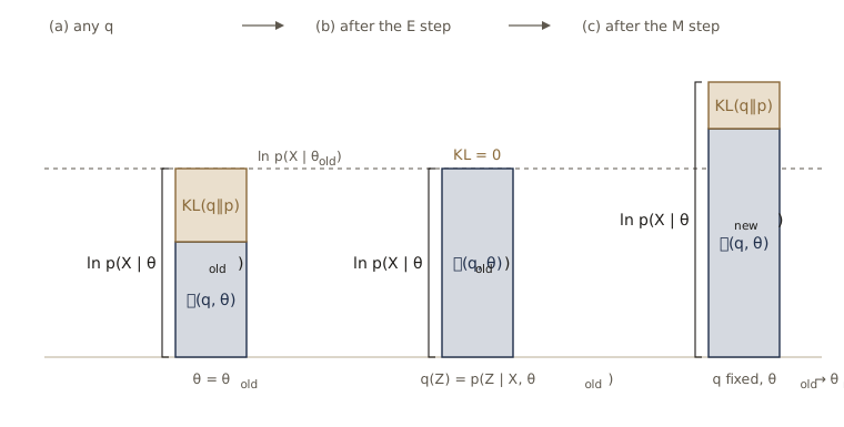
The same picture in parameter space
It helps to see the bound as a curve over the parameters. Take the simplest possible case: a one-dimensional mixture of two known unit-variance Gaussians at 0 and 2, with only the mixing coefficient \(\pi\) of the first component unknown. The data are 200 points in which 60% come from the first component. EM for \(\pi\) alone is: compute each point’s responsibility \(q_n\) for the first component, then set \(\pi\) to their average.
toy_rng = np.random.default_rng(6)
first = toy_rng.random(200) < 0.6  # 60% from the first component
x_toy = np.where(first, toy_rng.normal(0, 1, 200), toy_rng.normal(2, 1, 200))
log_a = -0.5 * np.log(2 * np.pi) - x_toy ** 2 / 2          # ln N(x_n | 0, 1)
log_b = -0.5 * np.log(2 * np.pi) - (x_toy - 2) ** 2 / 2    # ln N(x_n | 2, 1)

def toy_loglik(p):
    return np.sum(np.logaddexp(np.log(p) + log_a, np.log(1 - p) + log_b))

def toy_posterior(p):
    a1, a2 = np.log(p) + log_a, np.log(1 - p) + log_b
    return np.exp(a1 - np.logaddexp(a1, a2))

def toy_bound(q, p):
    """L(q, pi) with q_n = q(z_n = first component)."""
    return np.sum(q * (np.log(p) + log_a - np.log(q))
                  + (1 - q) * (np.log(1 - p) + log_b - np.log(1 - q)))

p = 0.1
for it in range(6):
    q = toy_posterior(p)                     # E step
    p_new = q.mean()                         # M step
    print(f"pi = {p:.4f}: ln p = {toy_loglik(p):.3f} -> bound max at {p_new:.4f} "
          f"(L = {toy_bound(q, p_new):.3f}), new ln p = {toy_loglik(p_new):.3f}")
    p = p_new

h, p0 = 1e-6, 0.1  # the bound touches ln p at pi_old with the same slope
q0 = toy_posterior(p0)
slope_lnp = (toy_loglik(p0 + h) - toy_loglik(p0 - h)) / (2 * h)
slope_L = (toy_bound(q0, p0 + h) - toy_bound(q0, p0 - h)) / (2 * h)
print(f"slope at pi = 0.1:  ln p {slope_lnp:.4f},  L(q_old, .) {slope_L:.4f}")
pi = 0.1000: ln p = -411.721 -> bound max at 0.2824 (L = -385.593), new ln p = -369.556
pi = 0.2824: ln p = -369.556 -> bound max at 0.4125 (L = -361.801), new ln p = -358.067
pi = 0.4125: ln p = -358.067 -> bound max at 0.4773 (L = -356.356), new ln p = -355.572
pi = 0.4773: ln p = -355.572 -> bound max at 0.5072 (L = -355.215), new ln p = -355.052
pi = 0.5072: ln p = -355.052 -> bound max at 0.5207 (L = -354.978), new ln p = -354.945
pi = 0.5207: ln p = -354.945 -> bound max at 0.5269 (L = -354.929), new ln p = -354.922
slope at pi = 0.1:  ln p 405.3189,  L(q_old, .) 405.3189
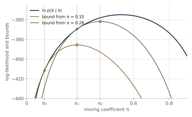
Each bound lies below the log-likelihood, touches it at the current parameter, and has the same slope there. The equal slopes are no accident: the gap \(\mathrm{KL}(q \Vert p(\mathbf{Z} \mid \mathbf{X}, \boldsymbol{\theta}))\) is zero at \(\boldsymbol{\theta}^{\mathrm{old}}\) and nonnegative everywhere, so \(\boldsymbol{\theta}^{\mathrm{old}}\) minimizes it and its gradient vanishes there. In this toy problem EM needs several steps because the two components overlap heavily: the responsibilities are far from 0 and 1, so each bound is much more sharply curved than the log-likelihood and its maximum is not far from the current point. When components are well separated, EM moves faster; when they overlap, it slows down. This is a general feature: EM’s convergence is linear, with a rate governed by how much information the latent variables hide.
MAP estimation with EM
With a prior \(p(\boldsymbol{\theta})\), we want to maximize \(\ln p(\boldsymbol{\theta} \mid \mathbf{X}) = \ln p(\mathbf{X} \mid \boldsymbol{\theta}) + \ln p(\boldsymbol{\theta}) - \ln p(\mathbf{X})\). The decomposition gives
\[\begin{aligned} \ln p(\boldsymbol{\theta} \mid \mathbf{X}) &= \mathcal{L}(q, \boldsymbol{\theta}) + \mathrm{KL}(q \Vert p) + \ln p(\boldsymbol{\theta}) - \ln p(\mathbf{X}) \\ &\ge \mathcal{L}(q, \boldsymbol{\theta}) + \ln p(\boldsymbol{\theta}) - \ln p(\mathbf{X}), \end{aligned}\]and \(\ln p(\mathbf{X})\) is a constant. We maximize the right side alternately over \(q\) and \(\boldsymbol{\theta}\). The prior does not involve \(q\), so the E step is unchanged; the M step maximizes \(\mathcal{Q}(\boldsymbol{\theta}, \boldsymbol{\theta}^{\mathrm{old}}) + \ln p(\boldsymbol{\theta})\), and every cycle increases the log posterior.
For the Gaussian mixture, a prior on each precision matrix of the form \(\ln p(\boldsymbol{\Lambda}_k) = \frac{a}{2} \ln \lvert \boldsymbol{\Lambda}_k \rvert - \frac{b}{2} \operatorname{Tr}(\boldsymbol{\Lambda}_k) + \text{const}\) (a Wishart density from module 02 with \(a + D + 1\) degrees of freedom and scale matrix \(b^{-1} \mathbf{I}\)) penalizes precisions that grow without bound. Adding it to the \(\boldsymbol{\Lambda}_k\) terms of \(\mathcal{Q}\) gives \(\frac{N_k + a}{2} \ln \lvert \boldsymbol{\Lambda}_k \rvert - \frac{1}{2} \operatorname{Tr}\left[ (N_k \mathbf{S}_k + b \mathbf{I}) \boldsymbol{\Lambda}_k \right]\), where \(\mathbf{S}_k\) is the maximum likelihood M-step covariance. Setting the derivative to zero,
\[\boldsymbol{\Sigma}_k^{\mathrm{new}} = \frac{N_k \mathbf{S}_k + b \mathbf{I}}{N_k + a}.\]However few points a component owns, its covariance is at least \(b / (N_k + a)\) times the identity. We rerun the collapsing example with \(a = 1\) and \(b = 0.1\).
def gmm_m_step_map(X, gamma, a=1.0, b=0.1):
    """M step with the prior (a/2) ln|Lambda_k| - (b/2) Tr(Lambda_k)."""
    pi, mu, S = gmm_m_step(X, gamma)
    N_k = gamma.sum(axis=0)[:, None, None]
    Sigma = (N_k * S + b * np.eye(X.shape[1])) / (N_k + a)
    return pi, mu, Sigma

def log_prior(Sigma, a=1.0, b=0.1):
    """Sum over k of (a/2) ln|Lambda_k| - (b/2) Tr(Lambda_k), Lambda_k = Sigma_k^-1."""
    total = 0.0
    for S in Sigma:
        Lam = np.linalg.solve(S, np.eye(len(S)))
        total += -a / 2 * np.linalg.slogdet(S)[1] - b / 2 * np.trace(Lam)
    return total

pi_c, mu_c = np.array([0.5, 0.5]), np.array([[0.0], [6.0]])
Sigma_c = np.array([[[1.0]], [[0.5]]])
objective = []
for it in range(30):
    gamma_c, ll_c = gmm_e_step(x_col, pi_c, mu_c, Sigma_c)
    objective.append(ll_c + log_prior(Sigma_c))
    if it in [0, 1, 2, 29]:
        print(f"iteration {it:2d}: variances {Sigma_c[:, 0, 0]}, means {mu_c.ravel()}, "
              f"objective {objective[-1]:.3f}")
    pi_c, mu_c, Sigma_c = gmm_m_step_map(x_col, gamma_c)
print("the objective ln p + ln prior never decreases:",
      bool(np.all(np.diff(objective) >= -1e-9)))
iteration  0: variances [1.  0.5], means [0. 6.], objective -46.000
iteration  1: variances [1.2124 0.0501], means [-0.0309  5.9999], objective -33.844
iteration  2: variances [1.2124 0.05  ], means [-0.0309  6.    ], objective -33.844
iteration 29: variances [1.2124 0.05  ], means [-0.0309  6.    ], objective -33.844
the objective ln p + ln prior never decreases: True
The second component still takes charge of the outlier, which is a reasonable reading of these data, but its variance stops at \(b / (N_k + a) = 0.1 / 2 = 0.05\) instead of collapsing to zero, and EM converges to a finite maximum of the posterior. The prior’s strength \(b\) should be small relative to the scale of the data; here the data have unit variance.
Generalized EM and incremental EM
EM splits a hard maximization into two easier ones, but for some models one of the two is still intractable. The bound view shows that neither step has to be complete.
Generalized EM (GEM) handles an intractable M step. Instead of maximizing \(\mathcal{L}(q, \boldsymbol{\theta})\) over \(\boldsymbol{\theta}\), it only increases it, for example with a few steps of a gradient-based optimizer. The argument above still applies: the bound goes up, so the log-likelihood goes up. A structured version, expectation conditional maximization (ECM), splits the parameters into groups and maximizes over one group at a time with the others fixed.
Partial E steps handle the other side. The E step need not set \(q\) all the way to the posterior; any change of \(q\) that increases \(\mathcal{L}\) keeps the algorithm climbing. Since \(\mathcal{L}(q, \boldsymbol{\theta}) \le \ln p(\mathbf{X} \mid \boldsymbol{\theta})\) with equality at the posterior, a global maximum of \(\mathcal{L}\) over both arguments gives a global maximum of the log-likelihood, and (for a continuous model) a local maximum of \(\mathcal{L}\) gives a local maximum of \(\ln p\). This view of EM as coordinate ascent on \(\mathcal{L}\) is due to Neal and Hinton.
One useful partial E step is incremental EM: update the responsibilities of a single data point, then do the M step right away. For exponential-family components this is cheap, because the M step depends on the responsibilities only through sufficient statistics, here \(N_k = \sum_n \gamma(z_{nk})\), \(\sum_n \gamma(z_{nk}) \mathbf{x}_n\), and \(\sum_n \gamma(z_{nk}) \mathbf{x}_n \mathbf{x}_n^{\mathrm{T}}\). When point \(m\)’s responsibility for component \(k\) changes from \(\gamma^{\mathrm{old}}(z_{mk})\) to \(\gamma^{\mathrm{new}}(z_{mk})\), each statistic changes by the difference times the point’s own contribution; for example
\[\begin{aligned} N_k^{\mathrm{new}} &= N_k^{\mathrm{old}} + \gamma^{\mathrm{new}}(z_{mk}) - \gamma^{\mathrm{old}}(z_{mk}), \\ \boldsymbol{\mu}_k^{\mathrm{new}} &= \boldsymbol{\mu}_k^{\mathrm{old}} + \frac{\gamma^{\mathrm{new}}(z_{mk}) - \gamma^{\mathrm{old}}(z_{mk})}{N_k^{\mathrm{new}}} \left( \mathbf{x}_m - \boldsymbol{\mu}_k^{\mathrm{old}} \right). \end{aligned}\]Each update costs a fixed amount of work, independent of \(N\), and the parameters improve after every point rather than after every pass. We compare passes of incremental EM (each pass is 300 single-point updates in random order) with batch iterations, starting both from the symmetric start of the Gaussian-mixture section, where batch EM crawls along a plateau.
def params_from_stats(N_k, S1, S2, N):
    """pi, mu, Sigma from the statistics sum gamma, sum gamma x, sum gamma x x^T."""
    mu = S1 / N_k[:, None]
    Sigma = S2 / N_k[:, None, None] - mu[:, :, None] * mu[:, None, :]
    return N_k / N, mu, Sigma

def one_point_responsibilities(x, pi, mu, Sigma):
    """gamma(z_k) for one point x, all K components at once (a lighter gmm_e_step)."""
    diff = x - mu                                                     # (K, D)
    sol = np.linalg.solve(Sigma, diff[:, :, None])[:, :, 0]  # Sigma_k^-1 (x - mu_k)
    maha = np.einsum("ki,ki->k", diff, sol)
    a = np.log(pi) - 0.5 * (np.linalg.slogdet(Sigma)[1] + maha)      # constants cancel
    g = np.exp(a - a.max())
    return g / g.sum()

def incremental_em(X, pi, mu, Sigma, passes, rng):
    N = len(X)
    gamma, _ = gmm_e_step(X, pi, mu, Sigma)  # one full E step to start
    N_k, S1 = gamma.sum(axis=0), gamma.T @ X
    S2 = np.einsum("nk,ni,nj->kij", gamma, X, X)
    pi, mu, Sigma = params_from_stats(N_k, S1, S2, N)
    loglik = []
    for _ in range(passes):
        for m in rng.permutation(N):
            x_m = X[m:m + 1]
            g_new = one_point_responsibilities(X[m], pi, mu, Sigma)  # partial E step
            d = g_new - gamma[m]
            gamma[m] = g_new
            N_k += d
            S1 += d[:, None] * x_m
            S2 += d[:, None, None] * (x_m.T @ x_m)
            pi, mu, Sigma = params_from_stats(N_k, S1, S2, N)        # M step
        loglik.append(gmm_loglik(X, pi, mu, Sigma))
    return loglik

_, _, ll_batch = gmm_em(X, pi0, mu_sym, Sigma0, max_iter=40, tol=-np.inf)
ll_inc = incremental_em(X, pi0, mu_sym, Sigma0, 20, np.random.default_rng(0))
for k in [1, 5, 10, 15, 20]:
    print(f"after {k:2d} passes: batch ln p = {ll_batch[k]:9.3f}   "
          f"incremental ln p = {ll_inc[k - 1]:9.3f}")
target = ll_batch[-1] - 1e-3
n_batch = int(np.argmax(np.array(ll_batch) > target))
n_inc = int(np.argmax(np.array(ll_inc) > target)) + 1
print("passes to get within 0.001 of the maximum: batch", n_batch, "incremental", n_inc)
after  1 passes: batch ln p =  -610.579   incremental ln p =  -609.979
after  5 passes: batch ln p =  -609.414   incremental ln p =  -608.503
after 10 passes: batch ln p =  -608.401   incremental ln p =  -605.233
after 15 passes: batch ln p =  -607.056   incremental ln p =  -455.931
after 20 passes: batch ln p =  -602.989   incremental ln p =  -405.477
passes to get within 0.001 of the maximum: batch 31 incremental 19
Incremental EM crosses the plateau in fewer passes over the data (19 against 31), because it acts on the improved parameters immediately instead of waiting for the end of a pass. Each of its passes costs more in Python here (300 small updates instead of one vectorized step), so the saving shows up most clearly for large data sets processed as a stream.
Note. The lower bound \(\mathcal{L}(q, \boldsymbol{\theta})\) is the seed of module 10. When the exact posterior \(p(\mathbf{Z} \mid \mathbf{X}, \boldsymbol{\theta})\) is too expensive to compute, we can still maximize \(\mathcal{L}\) over a restricted family of distributions \(q\). The gap \(\mathrm{KL}(q \Vert p)\) then no longer closes, but the bound remains a bound. That is variational inference, and treating the parameters themselves as latent variables in the same way gives the Bayesian mixture model without singularities.
Summary
| Method | Hidden quantity | E step | M step | Guarantee |
|---|---|---|---|---|
| K-means | cluster labels | nearest prototype | mean of each cluster | \(J\) never rises |
| K-medoids | cluster labels | least dissimilar prototype | best member of each cluster | \(\tilde{J}\) never rises |
| Gaussian mixture | component labels | responsibilities | weighted means, covariances, \(\pi_k\) | \(\ln p\) never falls |
| Bernoulli mixture | component labels | responsibilities | weighted pixel means, \(\pi_k\) | \(\ln p\) never falls |
| Bayesian regression | weights \(\mathbf{w}\) | posterior of \(\mathbf{w}\) | \(\alpha\) and \(\beta\) from its moments | evidence never falls |
| MAP, GEM, incremental | as above | exact or partial | maximize \(\mathcal{Q} + \ln p(\boldsymbol{\theta})\), or just improve \(\mathcal{L}\) | bound never falls |
Ideas to carry forward:
- A latent variable turns a hard marginal likelihood, with a sum inside the log, into an easy complete-data likelihood. EM exploits this by averaging the complete-data log-likelihood over the posterior of the latent variables (E step) and maximizing the average (M step).
- \(\ln p(\mathbf{X} \mid \boldsymbol{\theta}) = \mathcal{L}(q, \boldsymbol{\theta}) + \mathrm{KL}(q \Vert p)\): the E step closes the gap, the M step raises the bound, and the log-likelihood can only go up. Any step that raises the bound keeps this guarantee.
- EM finds local maxima, not global ones, and for Gaussian mixtures the likelihood has no global maximum at all. Initialization (K-means, several restarts), collapse detection, and priors are part of the method, not afterthoughts.
- K-means is EM with hard assignments, the small-variance limit of a Gaussian mixture; responsibilities are its soft generalization.
Exercises
- Show that K-means cannot cycle: prove that if the assignments at two different iterations are equal, then every assignment in between is equal too. Then give a one-dimensional data set of four points and an initialization for \(K = 2\) on which K-means stops at an assignment that is not the global minimum of \(J\). Confirm both claims with
kmeans. - Starting from the condition \(\partial J / \partial \boldsymbol{\mu}_k = \mathbf{0}\), use the Robbins–Monro method of module 02 to derive the online update for the prototypes. Then compare, in code, the step size \(1/(\text{count})\) used in
online_kmeanswith a constant step size \(\eta = 0.05\): plot \(J\) after each pass and explain why the constant step never settles exactly. - Suppose all components of a Gaussian mixture share one covariance matrix \(\boldsymbol{\Sigma}\). Derive the M-step update for \(\boldsymbol{\Sigma}\) (start from \(\mathcal{Q}\)). Modify
gmm_m_stepaccordingly, fit the geyser-like data, and compare the final log-likelihood with the full model. Which model would you expect to generalize better with only 30 points? - Derive the M step for a Gaussian mixture with diagonal covariances \(\boldsymbol{\Sigma}_k = \operatorname{diag}(\sigma_{k1}^2, \dots, \sigma_{kD}^2)\), and show that it is the diagonal of the full-covariance update.
- For a mixture \(p(\mathbf{x}) = \sum_k \pi_k p_k(\mathbf{x})\) whose components have means \(\boldsymbol{\mu}_k\) and covariances \(\boldsymbol{\Sigma}_k\), prove the formulas for \(\mathbb{E}[\mathbf{x}]\) and \(\operatorname{cov}[\mathbf{x}]\) used in the Bernoulli section. Check them numerically for the three-component Gaussian mixture
pi3, mu3, Sigma3by sampling. - Split \(\mathbf{x} = (\mathbf{x}_a, \mathbf{x}_b)\) and let \(p(\mathbf{x})\) be a Gaussian mixture. Show that the conditional \(p(\mathbf{x}_b \mid \mathbf{x}_a)\) is again a Gaussian mixture, and give its mixing coefficients and components. (Use the conditional Gaussian formulas of module 02 for each component.) Interpret the new mixing coefficients as responsibilities.
- Show that at any fixed point of EM for a Bernoulli mixture, the model mean \(\sum_k \pi_k \boldsymbol{\mu}_k\) equals the sample mean of the data. What happens if EM is started with all \(\boldsymbol{\mu}_k\) equal? Predict the result, then run
bernoulli_emwith such a start (you will need to add an argument for the initial means). - Put a beta prior \(\mathrm{Beta}(\mu_{ki} \mid a, b)\) on every pixel probability and a symmetric Dirichlet prior on \(\boldsymbol{\pi}\). Derive the MAP-EM updates, implement them, and show that with \(a = b = 2\) the clipping in
bernoulli_log_jointis no longer needed. How do the learned means change? - Derive the EM update for \(\beta\) in Bayesian linear regression from the expected complete-data log-likelihood, including the expectation of the squared error. Then start both iterations in the regression example from \(\alpha = 100, \beta = 0.1\) and from \(\alpha = 10^{-3}, \beta = 10^3\). Do they still agree? Which is faster?
- The bound \(\mathcal{L}(q, \boldsymbol{\theta})\) with \(q\) equal to the posterior at \(\boldsymbol{\theta}^{\mathrm{old}}\) has the same gradient as \(\ln p(\mathbf{X} \mid \boldsymbol{\theta})\) at \(\boldsymbol{\theta}^{\mathrm{old}}\). Prove this in general, then check it with central differences for the Gaussian mixture on the geyser-like data, differentiating with respect to the means at the poor starting parameters.
- Training log-likelihood cannot choose \(K\), because it keeps increasing as \(K\) grows. Split the geyser-like data into 200 training and 100 held-out points, fit mixtures with \(K = 1, \dots, 6\) (several starts each, K-means initialization), and plot training and held-out log-likelihood per point. What do you observe, and what happens to the largest \(K\) if you remove the restarts?
- In your own words: explain to a classmate why EM is guaranteed to improve the log-likelihood even though it never computes its gradient, and why this guarantee does not protect a Gaussian mixture from collapsing onto a single point.
Going further
- C. M. Bishop, Pattern Recognition and Machine Learning, chapter 9 — the source for this module. Exercises 9.1–9.2 treat K-means convergence and its online form, 9.6–9.9 the Gaussian-mixture M steps, 9.10 conditionals of mixtures, 9.12–9.19 Bernoulli and multinomial mixtures, 9.20–9.23 EM for regression hyperparameters and the relevance vector machine, and 9.24–9.27 the general EM bound and incremental EM.
- A. P. Dempster, N. M. Laird, and D. B. Rubin, “Maximum likelihood from incomplete data via the EM algorithm”, Journal of the Royal Statistical Society, Series B, 1977 — the paper that named EM and set it out in general.
- S. P. Lloyd, “Least squares quantization in PCM”, IEEE Transactions on Information Theory, 1982 — the batch K-means algorithm in its original setting, quantization for signal coding.
- R. M. Neal and G. E. Hinton, “A view of the EM algorithm that justifies incremental, sparse, and other variants,” in M. I. Jordan (ed.), Learning in Graphical Models, 1998 — EM as coordinate ascent on the lower bound, the view used in the last part of this module.
- G. J. McLachlan and T. Krishnan, The EM Algorithm and Extensions (Wiley) — a book-length treatment, including convergence rates and many variants.
- D. J. C. MacKay, Information Theory, Inference, and Learning Algorithms (Cambridge University Press, 2003; free to read on the author’s website), chapters 20 and 22 — K-means, soft K-means, and maximum likelihood for mixtures, with a different and very readable perspective.
These notes follow the chapters of C. M. Bishop, Pattern Recognition and Machine Learning (Springer, 2006), the course text, which Microsoft Research makes freely available as a PDF. The explanations, code, figures, and exercises here are written for this course; the book remains the reference, with the full derivations and many more exercises.