CSE 474/574 · Module 14 · Week 15
Combining Models
Model averaging versus combination, committees and bagging, AdaBoost as exponential-loss minimization, decision trees, and mixtures of experts.
Companion reading: Bishop, Pattern Recognition and Machine Learning, chapter 14, “Combining Models”
By the end of this module you can
- Tell Bayesian model averaging apart from model combination, and give a data set on which the two tell different stories.
- Build a bagged committee from bootstrap data sets, derive why averaging \(M\) models with uncorrelated errors divides the expected error by \(M\), and show that a committee is never worse than its average member.
- Implement AdaBoost with decision stumps from scratch, and derive its coefficients \(\alpha_m\) and its data-weight updates by minimizing the exponential error one stage at a time.
- Compare the exponential, cross-entropy, hinge, and misclassification error functions, and explain why the exponential error makes boosting sensitive to outliers and mislabeled points.
- Grow a regression or classification tree greedily with squared error, Gini index, or cross-entropy, and prune it by cost complexity.
- Explain what makes a tree easy to read and what makes it unstable, and demonstrate the instability on data.
- Fit a mixture of linear regressions, a mixture of logistic models, and a mixture of experts by EM, and relate them to decision trees and to the mixture density networks of module 05.
- Name the ideas that run through the whole course (likelihoods, priors, latent variables, approximations) and say where each one leads next.
Contents
- Bayesian model averaging versus model combination
- Committees
- Boosting
- Tree-based models
- Conditional mixture models
- Looking back over the course
- Summary
- Exercises
- Going further
Every module so far has built one model and fitted it as well as it could: a linear regression in module 03, a logistic classifier in module 04, a network in module 05, a mixture of Gaussians in module 09. This last module asks a different question. If we have several models, or can cheaply make several, is there a way to put them together that beats every one of them on its own?
There are two broad answers. The first is to let all the models vote and combine their outputs: a committee. We look at the simplest committee, which averages models trained on resampled copies of the data (bagging), and at a cleverer one, boosting, in which each new model is trained to fix the mistakes of the ones before it. The second answer is to let the input decide which model speaks. A decision tree does this with hard, axis-aligned questions; a mixture of experts does it softly, with input-dependent probabilities
\[p(t \mid \mathbf{x}) = \sum_{k=1}^{K} \pi_k(\mathbf{x})\, p(t \mid \mathbf{x}, k),\]in which the gating functions \(\pi_k(\mathbf{x}) = p(k \mid \mathbf{x})\) say how much model \(k\) is trusted at the input \(\mathbf{x}\).
Before any of this, we separate two ideas that sound alike and are easy to confuse: combining models, and averaging over our uncertainty about which model is true. The module ends with a look back over the whole course and a pointer to what comes next.
Bayesian model averaging versus model combination
Two generative stories
Take the mixture of Gaussians from module 09. Each data point \(\mathbf{x}_n\) has its own latent variable \(\mathbf{z}_n\) that says which component produced it, and the density of one point is
\[p(\mathbf{x}) = \sum_{\mathbf{z}} p(\mathbf{x}, \mathbf{z}) = \sum_{k=1}^{K} \pi_k\, \mathcal{N}(\mathbf{x} \mid \boldsymbol{\mu}_k, \boldsymbol{\Sigma}_k).\]For independent data the probability of the whole set \(\mathbf{X} = \{\mathbf{x}_1, \dots, \mathbf{x}_N\}\) is a product over points of a sum over components:
\[p(\mathbf{X}) = \prod_{n=1}^{N} \sum_{\mathbf{z}_n} p(\mathbf{x}_n, \mathbf{z}_n).\]The sum sits inside the product. Point 3 may come from component 1 and point 4 from component 2. This is model combination: the components are pieces of one model, and different data points can use different pieces.
Now suppose instead that we have \(H\) complete models, indexed by \(h\), with prior probabilities \(p(h)\). Perhaps one is a mixture of Gaussians and another a mixture of Student’s t distributions. Our uncertainty about which one is right gives
\[p(\mathbf{X}) = \sum_{h=1}^{H} p(\mathbf{X} \mid h)\, p(h) = \sum_{h=1}^{H} p(h) \prod_{n=1}^{N} p(\mathbf{x}_n \mid h).\]Here the sum sits outside the product. The story is that one model, chosen once, generated the entire data set; we just don’t know which. This is Bayesian model averaging, and it is the model comparison of module 03 carried through to prediction: the posterior \(p(h \mid \mathbf{X}) \propto p(\mathbf{X} \mid h)\, p(h)\) weights each model’s predictions,
\[p(\mathbf{x} \mid \mathbf{X}) = \sum_{h=1}^{H} p(\mathbf{x} \mid h)\, p(h \mid \mathbf{X}).\]As \(N\) grows, \(p(\mathbf{X} \mid h)\) is a product of more and more factors, so the ratios between models grow exponentially and the posterior concentrates on a single \(h\).
Note. The same distinction holds for conditional models \(p(t \mid \mathbf{x})\) and for predictive distributions. Ask of any “sum over models” whether the model index is drawn once for the whole data set (averaging over uncertainty) or once per data point (a latent variable inside a single, richer model).
An example where the difference matters
Let us make this concrete with two fixed densities on the real line, \(\mathcal{N}(x \mid -2, 1)\) and \(\mathcal{N}(x \mid 2, 1)\), each with probability one half. As a combination they form the mixture \(\tfrac12 \mathcal{N}(x \mid -2, 1) + \tfrac12 \mathcal{N}(x \mid 2, 1)\). As a model average they are two rival hypotheses about the whole data set. We generate two data sets: one in which every point picks its own component, and one in which all points come from the second density.
import numpy as np
from scipy.special import logsumexp, expit

np.set_printoptions(precision=4, suppress=True)
rng = np.random.default_rng(14)

def log_gauss(x, mu, sigma):
    """ln N(x | mu, sigma^2), elementwise with broadcasting."""
    return -0.5 * np.log(2 * np.pi * sigma**2) - 0.5 * ((x - mu) / sigma)**2

mus = np.array([-2.0, 2.0])            # the two candidate densities, unit variance
N = 100
z = rng.integers(0, 2, N)
x_mix = rng.normal(mus[z], 1.0)        # each point chooses its own component
x_one = rng.normal(mus[1], 1.0, N)     # the whole set comes from the second density

def log_p_combination(x):
    """ln p(X) under the 50/50 mixture: log-sum-exp over components, sum over points."""
    return logsumexp(np.log(0.5) + log_gauss(x[:, None], mus, 1.0), axis=1).sum()

def model_average(x):
    """Model averaging over h in {1, 2} with p(h) = 1/2: returns ln p(X), p(h | X)."""
    # ln p(h) + ln p(X | h) for each h
    log_joint = np.log(0.5) + log_gauss(x[:, None], mus, 1.0).sum(axis=0)
    log_pX = logsumexp(log_joint)
    return log_pX, np.exp(log_joint - log_pX)

for name, x in [("mixed data", x_mix), ("one-source data", x_one)]:
    print(name)
    for n in [1, 5, 20, 100]:
        log_pX_avg, post = model_average(x[:n])
        log_pX_comb = log_p_combination(x[:n])
        print(f"  N = {n:3d}   p(h=2 | X) = {post[1]:.4f}   ln p(X): "
              f"combination {log_pX_comb:8.2f}   averaging {log_pX_avg:8.2f}")
mixed data
  N =   1   p(h=2 | X) = 0.0000   ln p(X): combination    -2.30   averaging    -2.30
  N =   5   p(h=2 | X) = 0.0002   ln p(X): combination    -9.59   averaging   -25.10
  N =  20   p(h=2 | X) = 0.8155   ln p(X): combination   -37.95   averaging  -106.27
  N = 100   p(h=2 | X) = 1.0000   ln p(X): combination  -196.74   averaging  -504.69
one-source data
  N =   1   p(h=2 | X) = 0.6429   ln p(X): combination    -2.89   averaging    -2.89
  N =   5   p(h=2 | X) = 1.0000   ln p(X): combination    -9.92   averaging    -7.59
  N =  20   p(h=2 | X) = 1.0000   ln p(X): combination   -41.16   averaging   -29.02
  N = 100   p(h=2 | X) = 1.0000   ln p(X): combination  -209.96   averaging  -144.43
On the mixed data, the model average still insists that one density produced everything. Its posterior swings from one hypothesis to the other as points arrive, depending on which center the recent points happened to favor, and by \(N = 100\) it is certain of the second one, even though that hypothesis cannot explain the half of the points near \(-2\). Its log probability for the data, \(-504.69\), is far below the mixture’s \(-196.74\). On the one-source data the roles reverse. The average identifies the right density within five points, and at \(N = 100\) it beats the mixture by 65.5 nats, close to the \(N \ln 2 \approx 69.3\) that the mixture loses by spending half of its probability on a component the data never use.
The predictions differ in shape, not only in scale. After seeing the 100 mixed points:
_, post = model_average(x_mix)
for x0 in [-2.0, 0.0, 2.0]:
    p_comb = np.exp(logsumexp(np.log(0.5) + log_gauss(x0, mus, 1.0)))
    p_avg = np.sum(post * np.exp(log_gauss(x0, mus, 1.0)))
    print(f"x = {x0:4.1f}:  combination p(x) = {p_comb:.4f}   "
          f"averaging p(x | X) = {p_avg:.4f}")
x = -2.0:  combination p(x) = 0.1995   averaging p(x | X) = 0.0001
x =  0.0:  combination p(x) = 0.0540   averaging p(x | X) = 0.0540
x =  2.0:  combination p(x) = 0.1995   averaging p(x | X) = 0.3989
The mixture’s predictive density has two bumps. The averaged predictive density has one, at whichever center won, and it gives almost no probability to the other half of the data. Neither procedure is wrong in general; each is right when its generative story is right. Most of the methods in the rest of this module are forms of model combination.
Committees
Averaging reduces variance
Recall the bias–variance decomposition of module 03. When we fit the same flexible model to many independent data sets and average the fits, the variance part of the error shrinks while the bias stays put. The simplest committee does exactly this with \(M\) models \(y_1(\mathbf{x}), \dots, y_M(\mathbf{x})\):
\[y_{\mathrm{COM}}(\mathbf{x}) = \frac{1}{M} \sum_{m=1}^{M} y_m(\mathbf{x}).\]How much can averaging help? Let \(h(\mathbf{x})\) be the true regression function and write each model as the truth plus an error, \(y_m(\mathbf{x}) = h(\mathbf{x}) + \epsilon_m(\mathbf{x})\). Measure each model by its expected squared error over the input distribution, \(\mathbb{E}_{\mathbf{x}}[\epsilon_m(\mathbf{x})^2]\). The average error of the members acting alone, and the error of the committee, are
\[E_{\mathrm{AV}} = \frac{1}{M} \sum_{m=1}^{M} \mathbb{E}_{\mathbf{x}}\!\left[\epsilon_m(\mathbf{x})^2\right],\] \[E_{\mathrm{COM}} = \mathbb{E}_{\mathbf{x}}\!\left[\left(\frac{1}{M}\sum_{m=1}^{M} y_m(\mathbf{x}) - h(\mathbf{x})\right)^{2}\right] = \mathbb{E}_{\mathbf{x}}\!\left[\left(\frac{1}{M}\sum_{m=1}^{M} \epsilon_m(\mathbf{x})\right)^{2}\right].\]Expanding the square of the sum gives every product of two errors:
\[E_{\mathrm{COM}} = \frac{1}{M^2} \sum_{m=1}^{M} \mathbb{E}_{\mathbf{x}}\!\left[\epsilon_m^2\right] + \frac{1}{M^2} \sum_{m \ne l} \mathbb{E}_{\mathbf{x}}\!\left[\epsilon_m \epsilon_l\right].\]The first term is \(E_{\mathrm{AV}} / M\). If the errors are uncorrelated with zero mean, \(\mathbb{E}_{\mathbf{x}}[\epsilon_m \epsilon_l] = 0\) for \(m \ne l\), the second term vanishes, and
Result. With zero-mean, uncorrelated errors, \(E_{\mathrm{COM}} = \dfrac{1}{M} E_{\mathrm{AV}}\): averaging \(M\) models divides the expected squared error by \(M\).
That sounds too good, and it is. Models trained on the same data make similar mistakes, so their errors are positively correlated. Suppose each member has the same error \(\sigma^2 = \mathbb{E}_{\mathbf{x}}[\epsilon_m^2]\) and every pair has correlation \(\rho\), so \(\mathbb{E}_{\mathbf{x}}[\epsilon_m \epsilon_l] = \rho \sigma^2\). There are \(M(M-1)\) ordered pairs, so
\[E_{\mathrm{COM}} = \frac{\sigma^2}{M} + \frac{M(M-1)}{M^2}\, \rho \sigma^2 = \sigma^2 \left(\rho + \frac{1 - \rho}{M}\right).\]Only the uncorrelated fraction \(1 - \rho\) of the error is divided by \(M\); the correlated part \(\rho \sigma^2\) survives any amount of averaging.
There is also a guarantee that holds with no assumption at all. For any numbers \(a_1, \dots, a_M\) with mean \(\bar a\),
\[\frac{1}{M}\sum_{m} a_m^2 - \bar a^{\,2} = \frac{1}{M} \sum_{m} (a_m - \bar a)^2 \ge 0 .\]Apply this at each \(\mathbf{x}\) with \(a_m = \epsilon_m(\mathbf{x})\) and take the expectation:
\[E_{\mathrm{AV}} - E_{\mathrm{COM}} = \mathbb{E}_{\mathbf{x}}\!\left[\frac{1}{M} \sum_{m=1}^{M} \left(y_m(\mathbf{x}) - y_{\mathrm{COM}}(\mathbf{x})\right)^2\right] \ge 0 .\](The \(h(\mathbf{x})\) terms cancel inside the spread, since \(\epsilon_m - \bar\epsilon = y_m - y_{\mathrm{COM}}\).) So the committee is never worse than its average member, and it is better by exactly how much the members disagree. This identity is sometimes called the ambiguity decomposition. The inequality \(E_{\mathrm{COM}} \le E_{\mathrm{AV}}\) is a special case of Jensen’s inequality for the convex function \(x^2\), and it holds for any error that is convex in the prediction (exercise 1).
Let us check the correlated formula by simulation. We draw error vectors for \(M = 10\) members with a chosen correlation and compare the committee’s error with the formula.
def committee_errors(M, rho, sigma=1.0, S=200_000, rng=rng):
    """Draw S samples of M errors with variance sigma^2 and pairwise correlation rho."""
    common = rng.normal(0, 1, (S, 1))           # shared part: correlation rho
    own = rng.normal(0, 1, (S, M))              # private part
    eps = sigma * (np.sqrt(rho) * common + np.sqrt(1 - rho) * own)
    E_AV = np.mean(eps**2)
    E_COM = np.mean(eps.mean(axis=1)**2)
    return E_AV, E_COM

for rho in [0.0, 0.3, 0.8]:
    E_AV, E_COM = committee_errors(10, rho)
    print(f"rho = {rho:.1f}:  E_AV = {E_AV:.4f}   E_COM = {E_COM:.4f}   "
          f"formula = {E_AV * (rho + (1 - rho) / 10):.4f}")
rho = 0.0:  E_AV = 0.9974   E_COM = 0.0995   formula = 0.0997
rho = 0.3:  E_AV = 1.0031   E_COM = 0.3736   formula = 0.3711
rho = 0.8:  E_AV = 1.0007   E_COM = 0.8209   formula = 0.8206
With uncorrelated errors, ten members cut the error tenfold. With \(\rho = 0.8\) they cut it by less than a fifth.
Bagging
In practice we have one data set, not \(M\) independent ones. To get \(M\) different models we need a source of variety, and the bootstrap of module 01 provides it. A bootstrap data set is made by drawing \(N\) points from the original \(N\) with replacement; some points appear several times and others not at all. Bootstrap aggregation, or bagging, trains one copy of the model on each of \(M\) bootstrap data sets and averages their predictions (for classification, it takes a majority vote).
We try it on the running regression example of the course: 25 noisy observations of \(h(x) = \sin(2\pi x)\), fitted by a degree-9 polynomial with a small ridge penalty (module 03). Since we know \(h\), we can measure each model’s error \(\mathbb{E}_x[(y(x) - h(x))^2]\) exactly on a fine grid.
def h(x):
    return np.sin(2 * np.pi * x)

def poly_design(x, M):
    """Design matrix with columns 1, x, ..., x^M."""
    return np.vander(x, M + 1, increasing=True)

def fit_ridge(Phi, t, lam):
    """Regularized least squares: solve (lam I + Phi^T Phi) w = Phi^T t."""
    return np.linalg.solve(lam * np.eye(Phi.shape[1]) + Phi.T @ Phi, Phi.T @ t)

rng_bag = np.random.default_rng(11)
N_bag, degree, lam = 25, 9, 1e-4
x_bag = rng_bag.uniform(0, 1, N_bag)
t_bag = h(x_bag) + rng_bag.normal(0, 0.3, N_bag)
x_grid = np.linspace(0, 1, 400)
Phi_grid = poly_design(x_grid, degree)

w_full = fit_ridge(poly_design(x_bag, degree), t_bag, lam)
E_full = np.mean((Phi_grid @ w_full - h(x_grid))**2)

B = 200
Y = np.empty((B, len(x_grid)))                 # row m = y_m(x) on the grid
for m in range(B):
    idx = rng_bag.integers(0, N_bag, N_bag)     # a bootstrap data set
    Y[m] = Phi_grid @ fit_ridge(poly_design(x_bag[idx], degree), t_bag[idx], lam)

errors = Y - h(x_grid)                          # epsilon_m(x)
E_AV = np.mean(errors**2)
print(f"single model on all the data:  error {E_full:.4f}")
print(f"one bootstrap member, E_AV:    error {E_AV:.4f}")
for M in [5, 25, 200]:         # average over 100 random committees of M members
    E_M = np.mean([np.mean((Y[rng_bag.choice(B, M, replace=False)].mean(axis=0)
                            - h(x_grid))**2) for _ in range(100)])
    print(f"committee of M = {M:3d}:         error {E_M:.4f}")
single model on all the data:  error 0.0192
one bootstrap member, E_AV:    error 0.0739
committee of M =   5:         error 0.0256
committee of M =  25:         error 0.0195
committee of M = 200:         error 0.0180
The committee of 200 members is about four times better than a typical member (0.0180 against 0.0739), and most of the gain comes from the first few members. But the reduction is nowhere near a factor of 200, and the committee ends up only slightly better than a single model fitted to all 25 points (0.0192). Correlation explains the first fact. We can measure it: the average cross term relative to the average squared error plays the role of \(\rho\) above, and the formula then reproduces the committee error exactly.
G = errors @ errors.T / len(x_grid)             # G[m, l] = E_x[eps_m eps_l]
off_diag = G[~np.eye(B, dtype=bool)]
rho_hat = off_diag.mean() / np.diag(G).mean()
E_COM = np.mean((Y.mean(axis=0) - h(x_grid))**2)
print(f"effective correlation of member errors: {rho_hat:.3f}")
formula = E_AV * (rho_hat + (1 - rho_hat) / B)
print(f"E_AV (rho + (1 - rho)/M) = {formula:.4f}   E_COM = {E_COM:.4f}")
unique = np.mean([len(np.unique(rng_bag.integers(0, N_bag, N_bag))) / N_bag
                  for _ in range(2000)])
print(f"average fraction of distinct points in a bootstrap set: {unique:.3f}")
effective correlation of member errors: 0.240
E_AV (rho + (1 - rho)/M) = 0.0180   E_COM = 0.0180
average fraction of distinct points in a bootstrap set: 0.639
The members’ errors have an effective correlation of about 0.24, so no number of members can push the committee’s error below roughly \(0.24 \times 0.0739 \approx 0.018\), and 200 members are already there. The errors are correlated because every member is fitted to the same 25 points, and the parts of the fit that come from those points, noise included, are shared.
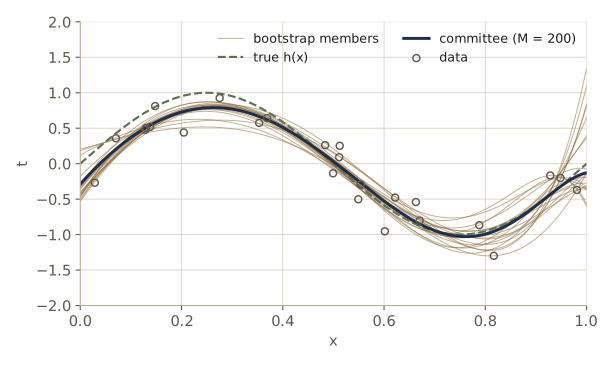
Watch out. Each bootstrap member sees only about 63% of the distinct data points (the printed fraction; the limit for large \(N\) is \(1 - e^{-1}\)), so a member is usually worse than one model fitted to all the data. The fair comparison for bagging is the single full-data model, not the average member. Bagging pays off for unstable procedures, whose fits change a lot when the data change a little. The smoothed polynomial here is only mildly unstable; the decision trees later in this module are very unstable, and bagging helps them far more.
The points left out of a bootstrap set, about a third of them, are a free validation set for that member. Predicting each training point with only the members that did not see it gives the out-of-bag error estimate, which comes at no extra cost (exercise 3).
Boosting
The idea
Bagging trains its members independently and hopes their errors are not too correlated. Boosting trains them in sequence and deliberately makes each one different: every new member is trained on a reweighted version of the data in which the points that the committee so far gets wrong count for more. The members are then combined by a weighted vote. The members can be very simple weak learners, classifiers only a little better than chance, and the committee can still be strong.
We look at the most widely used version, AdaBoost (“adaptive boosting”), for two classes with targets \(t_n \in \{-1, 1\}\). Each point carries a weight \(w_n\). We need a way to train a base classifier \(y(\mathbf{x}) \in \{-1, 1\}\) on weighted data, that is, to make its weighted error small.
Definition. AdaBoost trains \(M\) base classifiers one after another, each on a reweighted copy of the training set, and combines them by a weighted vote. Here \(I(\cdot)\) is the indicator function, 1 when its argument is true and 0 otherwise.
- Set the data weights to \(w_n^{(1)} = 1/N\) for \(n = 1, \dots, N\).
- For \(m = 1, \dots, M\):
- Train \(y_m(\mathbf{x})\) to minimize the weighted error \(J_m = \sum_n w_n^{(m)} I(y_m(\mathbf{x}_n) \ne t_n)\).
- Compute the weighted error rate \(\epsilon_m = \sum_n w_n^{(m)} I(y_m(\mathbf{x}_n) \ne t_n) \big/ \sum_n w_n^{(m)}\) and the member’s coefficient \(\alpha_m = \ln\{(1 - \epsilon_m)/\epsilon_m\}\).
- Reweight the data: \(w_n^{(m+1)} = w_n^{(m)} \exp\{\alpha_m I(y_m(\mathbf{x}_n) \ne t_n)\}\).
- Predict with \(Y_M(\mathbf{x}) = \operatorname{sign}\left(\sum_{m=1}^{M} \alpha_m y_m(\mathbf{x})\right)\).
When \(\epsilon_m < 1/2\), \(\alpha_m > 0\), so misclassified points have their weights multiplied by \(e^{\alpha_m} = (1 - \epsilon_m)/\epsilon_m > 1\) and correctly classified points keep theirs. Accurate members (small \(\epsilon_m\)) get large votes. The first member sees equal weights, so it is an ordinary classifier. Everything after that is shaped by what came before. We derive these particular formulas in the next subsection; first we run them.
Decision stumps
Our weak learner is a decision stump: a rule that looks at one input variable \(x_d\) and one threshold \(\theta\),
\[y(\mathbf{x}) = \begin{cases} s & \text{if } x_d > \theta, \\ -s & \text{otherwise,} \end{cases} \qquad s \in \{-1, 1\}.\]It is the smallest possible decision tree, one question deep, and it splits the plane with a line parallel to an axis. To fit it to weighted data we try every variable, every threshold between consecutive sorted values, and both signs. Sorting once per variable and taking cumulative sums of the weights gives the weighted error of every threshold at once.
def fit_stump(X, t, w):
    """Weighted stump: the (d, theta, s) minimizing sum_n w_n I(y(x_n) != t_n)."""
    N, D = X.shape
    best_err, best = np.inf, None
    for d in range(D):
        order = np.argsort(X[:, d])
        xs, ts, ws = X[order, d], t[order], w[order]
        # k points left of the threshold, k = 0..N. With s = +1 the left side
        # predicts -1, so the errors are the +1 points on the left and the -1 points
        # on the right.
        pos_left = np.concatenate([[0.0], np.cumsum(ws * (ts == 1))])
        neg_left = np.concatenate([[0.0], np.cumsum(ws * (ts == -1))])
        err_plus = pos_left + (neg_left[-1] - neg_left)
        err_minus = ws.sum() - err_plus               # s = -1 flips every prediction
        valid = np.r_[True, xs[1:] > xs[:-1], True]   # cut only between distinct values
        for s, err in ((1, err_plus), (-1, err_minus)):
            err = np.where(valid, err, np.inf)
            k = np.argmin(err)
            if err[k] < best_err:
                theta = (-np.inf if k == 0 else np.inf if k == N
                         else 0.5 * (xs[k - 1] + xs[k]))
                best_err, best = err[k], (d, theta, s)
    return best

def stump_predict(stump, X):
    d, theta, s = stump
    return np.where(X[:, d] > theta, s, -s)

# brute-force check on a tiny weighted problem
rng_chk = np.random.default_rng(0)
Xc = rng_chk.normal(size=(12, 2))
tc = np.where(rng_chk.random(12) < 0.5, 1, -1)
wc = rng_chk.random(12)
brute = min(np.sum(wc * (np.where(Xc[:, d] > th, s, -s) != tc))
            for d in range(2) for th in np.r_[Xc[:, d] - 1e-9, np.inf] for s in (1, -1))
fast = np.sum(wc * (stump_predict(fit_stump(Xc, tc, wc), Xc) != tc))
print(f"brute force {brute:.6f}   fit_stump {fast:.6f}")
brute force 1.710513 fit_stump 1.710513
AdaBoost on a two-dimensional problem
Our data set has one class in a disc and the other in a ring around it, with some overlap. Class \(+1\) has a radius drawn from a half-normal distribution with scale 0.7; class \(-1\) has a radius drawn from \(\mathcal{N}(1.6, 0.35^2)\); the angle is uniform. We train on 200 points and test on 2000.
def make_ring(N, rng):
    """Class +1 in a central disc, class -1 in a ring around it; t in {-1, +1}."""
    t = np.where(rng.random(N) < 0.5, 1, -1)
    r = np.where(t == 1, np.abs(rng.normal(0, 0.7, N)), rng.normal(1.6, 0.35, N))
    a = rng.uniform(0, 2 * np.pi, N)
    return np.c_[r * np.cos(a), r * np.sin(a)], t

rng_ring = np.random.default_rng(1)
X_ring, t_ring = make_ring(200, rng_ring)
X_ring_test, t_ring_test = make_ring(2000, rng_ring)

def adaboost(X, t, M):
    """AdaBoost with stumps: the stumps, their alphas, and the weights each one saw."""
    N = len(t)
    w = np.full(N, 1.0 / N)
    stumps, alphas, weights = [], [], []
    for m in range(M):
        stump = fit_stump(X, t, w)
        miss = stump_predict(stump, X) != t
        eps = w[miss].sum() / w.sum()
        eps = np.clip(eps, 1e-12, 1 - 1e-12)          # guard against a perfect stump
        alpha = np.log((1 - eps) / eps)
        stumps.append(stump); alphas.append(alpha); weights.append(w)
        w = w * np.exp(alpha * miss)
        w = w / w.sum()                        # rescaling changes nothing (see below)
    return stumps, np.array(alphas), np.array(weights)

def committee_score(stumps, alphas, X, m=None):
    """sum_{l <= m} alpha_l y_l(x): its sign is the AdaBoost prediction."""
    m = len(stumps) if m is None else m
    return sum(a * stump_predict(s, X) for s, a in zip(stumps[:m], alphas[:m]))

stumps, alphas, W_hist = adaboost(X_ring, t_ring, 300)
for m in [1, 2, 3, 5, 10, 20, 50, 100, 300]:
    train = np.mean(np.sign(committee_score(stumps, alphas, X_ring, m)) != t_ring)
    test = np.mean(np.sign(committee_score(stumps, alphas, X_ring_test, m)) !=
                   t_ring_test)
    print(f"m = {m:3d}:  training error {train:.3f}   test error {test:.4f}")
m =   1:  training error 0.335   test error 0.3565
m =   2:  training error 0.340   test error 0.3585
m =   3:  training error 0.175   test error 0.2240
m =   5:  training error 0.245   test error 0.2760
m =  10:  training error 0.135   test error 0.1755
m =  20:  training error 0.060   test error 0.1175
m =  50:  training error 0.050   test error 0.1115
m = 100:  training error 0.030   test error 0.1110
m = 300:  training error 0.000   test error 0.1125
One stump can only cut the plane in two, and it misclassifies about a third of the points. A few rounds later the committee has boxed in the disc, and by round 300 the training error is zero. The training error need not fall every round (it rose from round 3 to round 5); the quantity that falls every round is the exponential error of the next subsection. The test error drops quickly and then levels off near 11% rather than climbing back up, even though the committee keeps adding members long after it fits the training set almost perfectly.
How good is the plateau? Since we know how the data were generated, we can compute the error of the best possible classifier, the Bayes error of module 01. The class-conditional densities depend on the radius only, so the optimal rule compares the two radial densities.
r = np.linspace(0, 4, 40_001)
f_plus = 2 * np.exp(log_gauss(r, 0.0, 0.7))        # half-normal radius, class +1
f_minus = np.exp(log_gauss(r, 1.6, 0.35))          # ring radius, class -1
bayes_error = 0.5 * np.sum(np.minimum(f_plus, f_minus)) * (r[1] - r[0])
print(f"Bayes error {bayes_error:.4f}")
Bayes error 0.0957
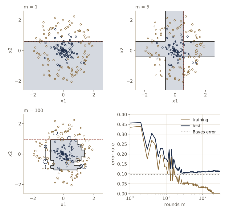
Note. A sum of stumps is a sum of functions of one variable each, \(g_1(x_1) + g_2(x_2)\). Our optimal boundary, a circle \(x_1^2 + x_2^2 = c\), has exactly that form, which is why boosted stumps approximate it so well. A boundary that depends on a product such as \(x_1 x_2\) cannot be written this way; boosting deeper trees (two questions each) captures such interactions.
Minimizing exponential error
Where do the formulas for \(\alpha_m\) and the weights come from? A clean answer is that AdaBoost minimizes a particular error function, one member at a time. Define the committee score and the exponential error
\[f_m(\mathbf{x}) = \frac{1}{2} \sum_{l=1}^{m} \alpha_l\, y_l(\mathbf{x}), \qquad E = \sum_{n=1}^{N} \exp\{-t_n f_m(\mathbf{x}_n)\}.\]The product \(t_n f_m(\mathbf{x}_n)\) is positive when the committee classifies point \(n\) correctly and grows with its confidence, so \(E\) is small when all points are classified correctly with a margin. Minimizing \(E\) jointly over all members is hard. Instead, we keep \(y_1, \dots, y_{m-1}\) and \(\alpha_1, \dots, \alpha_{m-1}\) fixed and minimize over the newest member \(y_m\) and its coefficient \(\alpha_m\) only. This is called stagewise fitting.
Pull the old members out of the exponent:
\[\begin{aligned} E &= \sum_{n=1}^{N} \exp\{-t_n f_{m-1}(\mathbf{x}_n)\} \exp\left\{-\tfrac12 t_n \alpha_m y_m(\mathbf{x}_n)\right\} \\ &= \sum_{n=1}^{N} w_n^{(m)} \exp\left\{-\tfrac12 t_n \alpha_m y_m(\mathbf{x}_n)\right\}, \end{aligned}\]where \(w_n^{(m)} = \exp\{-t_n f_{m-1}(\mathbf{x}_n)\}\) does not depend on the new member. These are the data weights. Since \(t_n y_m(\mathbf{x}_n)\) is \(+1\) for a correct point and \(-1\) for a wrong one, split the sum into the correctly classified set \(\mathcal{T}_m\) and the misclassified set \(\mathcal{M}_m\):
\[\begin{aligned} E &= e^{-\alpha_m/2} \sum_{n \in \mathcal{T}_m} w_n^{(m)} + e^{\alpha_m/2} \sum_{n \in \mathcal{M}_m} w_n^{(m)} \\ &= \left(e^{\alpha_m/2} - e^{-\alpha_m/2}\right) \sum_{n=1}^{N} w_n^{(m)} I(y_m(\mathbf{x}_n) \ne t_n) + e^{-\alpha_m/2} \sum_{n=1}^{N} w_n^{(m)} . \end{aligned}\]The member. For any \(\alpha_m > 0\), the second term does not involve \(y_m\) and the factor in front of the first is positive. So the best \(y_m\) minimizes the weighted error \(J_m\), step 2 of the algorithm.
The coefficient. Divide by \(\sum_n w_n^{(m)}\) and write \(\epsilon_m\) for the weighted error rate; then \(E \propto (1 - \epsilon_m) e^{-\alpha_m/2} + \epsilon_m e^{\alpha_m/2}\). Setting the derivative with respect to \(\alpha_m\) to zero,
\[-\tfrac12 (1 - \epsilon_m) e^{-\alpha_m/2} + \tfrac12 \epsilon_m e^{\alpha_m/2} = 0 \quad\Longrightarrow\quad e^{\alpha_m} = \frac{1 - \epsilon_m}{\epsilon_m}, \qquad \alpha_m = \ln \frac{1 - \epsilon_m}{\epsilon_m}.\]The second derivative is positive, so this is a minimum.
The weights. The next round’s weights are \(w_n^{(m+1)} = \exp\{-t_n f_m(\mathbf{x}_n)\} = w_n^{(m)} \exp\{-\tfrac12 t_n \alpha_m y_m(\mathbf{x}_n)\}\). Use \(t_n y_m(\mathbf{x}_n) = 1 - 2 I(y_m(\mathbf{x}_n) \ne t_n)\):
\[w_n^{(m+1)} = w_n^{(m)}\, e^{-\alpha_m/2} \exp\{\alpha_m I(y_m(\mathbf{x}_n) \ne t_n)\}.\]The factor \(e^{-\alpha_m/2}\) is the same for every point. Rescaling all weights by a common factor changes neither the next weighted fit nor the next \(\epsilon\), so we may drop it, which gives exactly the AdaBoost update. Finally, \(f_M\) and \(2 f_M = \sum_m \alpha_m y_m\) have the same sign, which gives the prediction rule. Every step of AdaBoost is accounted for.
The derivation also tells us how fast the error falls. Substituting the optimal \(\alpha_m\) back, with \(e^{\alpha_m/2} = \sqrt{(1 - \epsilon_m)/\epsilon_m}\),
\[E_m = E_{m-1}\left[(1 - \epsilon_m) \sqrt{\frac{\epsilon_m}{1 - \epsilon_m}} + \epsilon_m \sqrt{\frac{1 - \epsilon_m}{\epsilon_m}}\right] = 2\sqrt{\epsilon_m (1 - \epsilon_m)}\; E_{m-1},\]and \(2\sqrt{\epsilon (1 - \epsilon)} < 1\) whenever \(\epsilon \ne 1/2\). Because \(e^{-z} \ge 1\) whenever \(z \le 0\), every misclassified point contributes at least 1 to \(E\), so the number of training mistakes is at most \(E_M = N \prod_{m} 2\sqrt{\epsilon_m(1 - \epsilon_m)}\). As long as each weak learner beats chance by some margin, the training error is driven to zero exponentially fast.
Let us check these claims on the run above: that \(\alpha_3\) minimizes \(E\) along a grid, that the error ratio matches \(2\sqrt{\epsilon(1-\epsilon)}\), and that the bound holds.
def exp_error(stumps, alphas, X, t, m):
    """E = sum_n exp(-t_n f_m(x_n)) with f_m = (1/2) sum_{l <= m} alpha_l y_l."""
    return np.sum(np.exp(-t * 0.5 * committee_score(stumps, alphas, X, m)))

m = 3                                          # check the third round
w_m = np.exp(-t_ring * 0.5 * committee_score(stumps, alphas, X_ring, m - 1))
y_m = stump_predict(stumps[m - 1], X_ring)
grid = np.linspace(0.01, 3, 3000)
E_grid = [np.sum(w_m * np.exp(-0.5 * t_ring * a * y_m)) for a in grid]
print(f"alpha_3 from the formula {alphas[m - 1]:.4f}   "
      f"grid minimizer {grid[np.argmin(E_grid)]:.4f}")

E = [exp_error(stumps, alphas, X_ring, t_ring, m) for m in range(301)]   # E_0..E_300
eps = np.array([W_hist[l][stump_predict(stumps[l], X_ring) != t_ring].sum()
                for l in range(300)])                  # eps[m - 1] = epsilon_m
for m in [1, 10, 100]:
    factor = 2 * np.sqrt(eps[m - 1] * (1 - eps[m - 1]))
    print(f"m = {m:3d}: E_m / E_(m-1) = {E[m] / E[m - 1]:.4f}   "
          f"2 sqrt(eps (1 - eps)) = {factor:.4f}")
for m in [10, 50, 100]:
    mistakes = np.sum(np.sign(committee_score(stumps, alphas, X_ring, m)) != t_ring)
    print(f"m = {m:3d}: training mistakes {mistakes:3d}  <=  bound E_m = {E[m]:7.2f}")
alpha_3 from the formula 0.7214   grid minimizer 0.7219
m =   1: E_m / E_(m-1) = 0.9440   2 sqrt(eps (1 - eps)) = 0.9440
m =  10: E_m / E_(m-1) = 0.9719   2 sqrt(eps (1 - eps)) = 0.9719
m = 100: E_m / E_(m-1) = 0.9898   2 sqrt(eps (1 - eps)) = 0.9898
m =  10: training mistakes  27  <=  bound E_m =  119.67
m =  50: training mistakes  10  <=  bound E_m =   55.17
m = 100: training mistakes   6  <=  bound E_m =   35.29
(In adaboost we normalized the weights to sum to one, so W_hist[l] sums to one and the weighted error rate is a plain sum.) The weak learners here really are weak: the later ones have \(\epsilon_m\) close to one half, so each round shrinks \(E\) only a little, but the shrinking never stops.
Watch out. Zero training error is not the goal, and the bound says nothing about test error. On noisy data AdaBoost will eventually fit the noise; the plateau we saw is typical when the classes overlap only moderately, but on harder problems the test error does rise again. In practice the number of rounds \(M\) is chosen on a validation set, and each new member is often shrunk by a factor \(\nu < 1\) before it is added.
Error functions for boosting
What does minimizing the exponential error aim at? Imagine unlimited data and a completely flexible function \(y(\mathbf{x})\). The expected error is
\[\mathbb{E}_{\mathbf{x}, t}\left[e^{-t y(\mathbf{x})}\right] = \int \left\{ p(t{=}1 \mid \mathbf{x})\, e^{-y(\mathbf{x})} + p(t{=}{-1} \mid \mathbf{x})\, e^{y(\mathbf{x})} \right\} p(\mathbf{x})\, d\mathbf{x}.\]We can choose \(y(\mathbf{x})\) separately at each \(\mathbf{x}\), so we minimize the braces pointwise. Setting the derivative with respect to \(y\) to zero, \(-p(t{=}1 \mid \mathbf{x}) e^{-y} + p(t{=}{-1} \mid \mathbf{x}) e^{y} = 0\), gives
\[y^{\star}(\mathbf{x}) = \frac{1}{2} \ln \frac{p(t = 1 \mid \mathbf{x})}{p(t = -1 \mid \mathbf{x})},\]half the log odds. So AdaBoost is estimating the log odds, within the family of weighted sums of stumps and with the restriction of fitting one member at a time. Its sign is the Bayes-optimal decision, and inverting the relation gives a class probability, \(p(t = 1 \mid \mathbf{x}) = \sigma(2 y^{\star}(\mathbf{x}))\) with the logistic sigmoid \(\sigma\).
Logistic regression (module 04) estimates the same log odds with a different error. Write the targets as \(t \in \{-1, 1\}\) and the model’s score as \(y\), so that \(p(t \mid \mathbf{x}) = \sigma(t y)\). The negative log likelihood of one point is then \(\ln(1 + e^{-t y})\), the cross-entropy error in this notation. In terms of the margin \(z = t y(\mathbf{x})\), we can compare four error functions:
| Error | \(E(z)\) | Used by |
|---|---|---|
| misclassification | \(1\) if \(z < 0\), else \(0\) | what we really care about |
| exponential | \(e^{-z}\) | AdaBoost |
| cross-entropy (rescaled) | \(\ln(1 + e^{-z}) / \ln 2\) | logistic regression (module 04) |
| hinge | \(\max(0, 1 - z)\) | support vector machines (module 07) |
The cross-entropy is divided by \(\ln 2\) so that all the smooth ones pass through \((0, 1)\).
z = np.array([-4.0, -2.0, -1.0, 0.0, 1.0, 2.0])
losses = {
    "misclassification": (z < 0).astype(float),
    "exponential":       np.exp(-z),
    "cross-entropy/ln2": np.logaddexp(0, -z) / np.log(2),
    "hinge":             np.maximum(0, 1 - z),
}
print("z:                 " + "".join(f"{v:8.1f}" for v in z))
for name, E in losses.items():
    print(f"{name:19s}" + "".join(f"{v:8.3f}" for v in E))
z:                     -4.0    -2.0    -1.0     0.0     1.0     2.0
misclassification     1.000   1.000   1.000   0.000   0.000   0.000
exponential          54.598   7.389   2.718   1.000   0.368   0.135
cross-entropy/ln2     5.797   3.069   1.895   1.000   0.452   0.183
hinge                 5.000   3.000   2.000   1.000   0.000   0.000
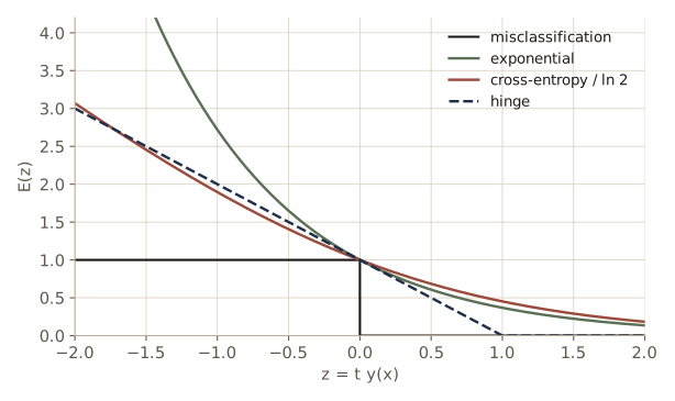
All three smooth errors are convex and sit above the step, so each is a usable surrogate for misclassification. They part ways for large negative margins. At \(z = -4\) the exponential error is about 55 while the cross-entropy is about 6. A point that is confidently on the wrong side, such as an outlier or a mislabeled point, therefore dominates the exponential error, and AdaBoost will spend round after round on it. We can see this directly by flipping the labels of 5% of the training points and watching where the weight goes.
rng_flip = np.random.default_rng(2)
flipped = rng_flip.choice(len(t_ring), size=10, replace=False)
t_noisy = t_ring.copy()
t_noisy[flipped] *= -1

stumps_n, alphas_n, W_n = adaboost(X_ring, t_noisy, 300)
for m in [1, 10, 50, 100, 300]:
    share = W_n[m - 1][flipped].sum()                 # weights sum to one
    test = np.mean(np.sign(committee_score(stumps_n, alphas_n, X_ring_test, m)) !=
                   t_ring_test)
    print(f"m = {m:3d}:  weight on the 10 flipped points {share:.3f}   "
          f"test error {test:.4f}")
m =   1:  weight on the 10 flipped points 0.050   test error 0.3540
m =  10:  weight on the 10 flipped points 0.120   test error 0.1725
m =  50:  weight on the 10 flipped points 0.207   test error 0.1160
m = 100:  weight on the 10 flipped points 0.231   test error 0.1220
m = 300:  weight on the 10 flipped points 0.236   test error 0.1250
Ten points out of 200 start with 5% of the weight and end up holding nearly a quarter of it. A large part of every later stump’s job is to accommodate them, and the test error after 300 rounds is 12.5%, against 11.25% on clean data. The damage here is modest because only a few labels were flipped, but the mechanism is the one to remember: under the exponential error, the points that are most wrong get the most attention, whether or not they deserve it.
Two more differences are worth knowing. The cross-entropy is the negative log of a normalized probability model, the logistic model, so it comes with a likelihood, calibrated probabilities, and a natural extension to \(K > 2\) classes through the softmax of module 04. The exponential error is not the negative log likelihood of any properly normalized model: if it were, \(p(t \mid \mathbf{x})\) would be proportional to \(\exp(-e^{-t y})\), and those two values do not sum to one for general \(y\) (exercise 6). The attraction of the exponential error is the one we derived: stagewise minimization yields the simple reweighting scheme.
Boosting for regression
The stagewise view suggests boosting with other errors. With the sum-of-squares error \(E = \frac12 \sum_n \{t_n - f_{m-1}(\mathbf{x}_n) - y_m(\mathbf{x}_n)\}^2\) (absorbing the coefficient into \(y_m\)), the new member minimizes
\[\frac12 \sum_{n=1}^{N} \left\{ r_n^{(m)} - y_m(\mathbf{x}_n) \right\}^2, \qquad r_n^{(m)} = t_n - f_{m-1}(\mathbf{x}_n),\]so each member is fitted to the residuals that the committee has left so far. Here is that recipe with one-variable regression stumps (a threshold, and a constant on each side) on noisy sine data, shrinking each member by \(\nu = 0.3\):
def fit_reg_stump(x, r):
    """Least-squares stump on one input: threshold and a mean on each side."""
    order = np.argsort(x); xs, rs = x[order], r[order]
    k = np.arange(1, len(x))                                  # points on the left
    s_left = np.cumsum(rs)[:-1]
    s_right, n_right = rs.sum() - s_left, len(x) - k
    sse = -(s_left**2 / k) - (s_right**2 / n_right)          # SSE up to a constant
    sse = np.where(xs[1:] > xs[:-1], sse, np.inf)
    j = np.argmin(sse)
    return 0.5 * (xs[j] + xs[j + 1]), s_left[j] / k[j], s_right[j] / n_right[j]

rng_reg = np.random.default_rng(4)
x_reg = rng_reg.uniform(0, 1, 100)
t_reg = h(x_reg) + rng_reg.normal(0, 0.3, 100)

nu, f_train, f_grid = 0.3, np.zeros(100), np.zeros(len(x_grid))
for m in range(1, 201):
    theta, left, right = fit_reg_stump(x_reg, t_reg - f_train)       # fit the residuals
    f_train += nu * np.where(x_reg <= theta, left, right)
    f_grid += nu * np.where(x_grid <= theta, left, right)
    if m in (1, 10, 50, 200):
        rms = np.sqrt(np.mean((t_reg - f_train)**2))
        print(f"m = {m:3d}:  training RMS {rms:.3f}   "
              f"error vs h {np.mean((f_grid - h(x_grid))**2):.4f}")
m =   1:  training RMS 0.582   error vs h 0.3115
m =  10:  training RMS 0.358   error vs h 0.0682
m =  50:  training RMS 0.263   error vs h 0.0116
m = 200:  training RMS 0.223   error vs h 0.0137
The error against \(h\) falls to about 0.012 by round 50 and then creeps up again as the members start fitting noise, which is why the number of rounds is chosen on validation data. This is the core of gradient boosting, which generalizes the residual to the negative gradient of any differentiable error. For regression, the squared error has the same weakness as the exponential error has for classification: large residuals dominate. Boosting with the absolute error \(\lvert y - t \rvert\), which grows only linearly, is more robust to outliers.
Tree-based models
Partitioning the input space
A different way to combine simple models is to give each one its own region of input space. A decision tree splits the input space into axis-aligned boxes by asking a sequence of yes/no questions of the form “is \(x_d \le \theta\)?”, and fits a very simple model (a constant) in each box. The questions are arranged as a binary tree: every internal node holds one question and sends the input left or right; every leaf \(\tau\) holds a region \(\mathcal{R}_\tau\) and a prediction \(y_\tau\). For a new input we start at the root and follow the answers down to a leaf. As a model,
\[y(\mathbf{x}) = \sum_{\tau=1}^{\lvert T \rvert} y_\tau\, I(\mathbf{x} \in \mathcal{R}_\tau),\]where \(\lvert T \rvert\) is the number of leaves of the tree \(T\). Each point is handled by exactly one leaf, so this is a combination of models in which the input selects a single member. (Despite the drawing, a decision tree is not a graphical model in the sense of module 08; its nodes are questions, not random variables.) We follow the CART framework (classification and regression trees); ID3 and C4.5 are well-known relatives that differ in details.
Growing a tree greedily
To learn a tree we must choose its shape, the variable and threshold at each internal node, and the leaf values.
The leaf values are easy once the regions are fixed. For regression with squared error, the best constant for the \(N_\tau\) points in region \(\mathcal{R}_\tau\) minimizes \(\sum_{\mathbf{x}_n \in \mathcal{R}_\tau} (t_n - y_\tau)^2\); setting the derivative \(-2\sum (t_n - y_\tau)\) to zero gives the mean,
\[y_\tau = \frac{1}{N_\tau} \sum_{\mathbf{x}_n \in \mathcal{R}_\tau} t_n, \qquad Q_\tau(T) = \sum_{\mathbf{x}_n \in \mathcal{R}_\tau} (t_n - y_\tau)^2,\]where \(Q_\tau\) is the leaf’s residual sum of squares. For classification, a leaf predicts its majority class and its quality is measured by how mixed its classes are. With \(p_{\tau k}\) the fraction of the leaf’s points in class \(k\), the two usual impurity measures are
\[\text{cross-entropy: } -\sum_{k=1}^{K} p_{\tau k} \ln p_{\tau k}, \qquad \text{Gini index: } \sum_{k=1}^{K} p_{\tau k}(1 - p_{\tau k}).\]Both are zero for a pure leaf and largest when the classes are evenly mixed. To compare splits we weight a leaf’s impurity by its size, \(N_\tau\) times the impurity, so that a large impure leaf counts for more than a small one.
The shape is the hard part: finding the best tree of a given size is a combinatorial search that is infeasible except for tiny problems. CART grows the tree greedily instead. Start with one leaf holding all the data. For a leaf, try every input variable and every threshold between consecutive distinct values, and keep the split whose two children have the smallest total cost; repeat on the children. For one variable, sorting the points and keeping running sums of the sufficient statistics (count, sum, and sum of squares for regression; class counts for classification) gives the cost of all thresholds in one pass, so a split search costs \(O(D N \log N)\).
def node_cost(S, kind):
    """N_tau times the impurity, for nodes with sufficient statistics S (last axis).
    kind "sse": S = (n, sum t, sum t^2).  "gini" or "entropy": S = class counts."""
    if kind == "sse":
        n, s1, s2 = S[..., 0], S[..., 1], S[..., 2]
        return s2 - s1**2 / np.maximum(n, 1)
    n = S.sum(axis=-1)
    p = S / np.maximum(n, 1)[..., None]
    if kind == "gini":
        Q = np.sum(p * (1 - p), axis=-1)
    else:
        Q = -np.sum(p * np.log(np.where(p > 0, p, 1.0)), axis=-1)
    return n * Q

def suff_stats(t, kind, K=2):
    """Per-point statistics: (1, t, t^2) for regression, one-hot rows for classes."""
    return np.c_[np.ones(len(t)), t, t**2] if kind == "sse" else np.eye(K)[t]

def best_split(X, S, kind, min_leaf):
    """Best (cost, variable, threshold) over all splits, or (inf, None, None)."""
    N, D = X.shape
    best = (np.inf, None, None)
    for d in range(D):
        order = np.argsort(X[:, d], kind="stable")
        xs = X[order, d]
        left = np.cumsum(S[order], axis=0)[:-1]    # stats of the k leftmost points
        cost = node_cost(left, kind) + node_cost(S.sum(axis=0) - left, kind)
        k = np.arange(1, N)
        ok = (xs[1:] > xs[:-1]) & (k >= min_leaf) & (N - k >= min_leaf)
        if ok.any():
            j = np.argmin(np.where(ok, cost, np.inf))
            if cost[j] < best[0]:
                best = (cost[j], d, 0.5 * (xs[j] + xs[j + 1]))
    return best

def grow(X, S, kind, min_leaf=5, max_depth=20, depth=0):
    """Grow a tree greedily. Nodes are dicts; internal nodes add d, theta, children."""
    stats = S.sum(axis=0)
    node = {"n": len(X), "stats": stats, "cost": float(node_cost(stats, kind))}
    if depth < max_depth and len(X) >= 2 * min_leaf and node["cost"] > 1e-12:
        _, d, theta = best_split(X, S, kind, min_leaf)
        if d is not None:
            go_left = X[:, d] <= theta
            args = (kind, min_leaf, max_depth, depth + 1)
            node.update(d=d, theta=theta,
                        left=grow(X[go_left], S[go_left], *args),
                        right=grow(X[~go_left], S[~go_left], *args))
    return node

def leaf_value(node, kind):
    s = node["stats"]
    return s[1] / s[0] if kind == "sse" else np.argmax(s)

def predict_tree(node, X, kind):
    """Send every row of X down the tree, all rows that reach a node at once."""
    out = np.empty(len(X))
    def walk(nd, idx):
        if "d" not in nd:
            out[idx] = leaf_value(nd, kind)
            return
        go_left = X[idx, nd["d"]] <= nd["theta"]
        walk(nd["left"], idx[go_left])
        walk(nd["right"], idx[~go_left])
    walk(node, np.arange(len(X)))
    return out

def n_leaves(node):
    return 1 if "d" not in node else n_leaves(node["left"]) + n_leaves(node["right"])

def show_tree(node, kind, indent=""):
    if "d" not in node:
        s = node["stats"]
        value = (f"mean {s[1] / s[0]:.3f}" if kind == "sse"
                 else f"counts {s.astype(int)}")
        print(f"{indent}leaf: n = {node['n']}, {value}")
    else:
        print(f"{indent}x{node['d'] + 1} <= {node['theta']:.3f}?")
        show_tree(node["left"], kind, indent + "    ")
        show_tree(node["right"], kind, indent + "    ")
We grow a small classification tree on the ring data (classes coded 0 for the ring and 1 for the disc) with the Gini index, limited to depth 3 so that we can read it.
c_ring = (t_ring == 1).astype(int)                 # class 1 = disc, class 0 = ring
c_ring_test = (t_ring_test == 1).astype(int)
tree3 = grow(X_ring, suff_stats(c_ring, "gini"), "gini", min_leaf=5, max_depth=3)
show_tree(tree3, "gini")
test_err = np.mean(predict_tree(tree3, X_ring_test, "gini") != c_ring_test)
print(f"leaves {n_leaves(tree3)}   test error {test_err:.4f}")
x2 <= -1.051?
    leaf: n = 29, counts [29  0]
    x2 <= 0.609?
        x1 <= 1.178?
            leaf: n = 109, counts [17 92]
            leaf: n = 15, counts [14  1]
        x2 <= 1.068?
            leaf: n = 16, counts [10  6]
            leaf: n = 31, counts [30  1]
leaves 5   test error 0.1810
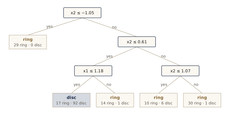
Read it from the top. The first question carves off the bottom of the ring, where every point is class 0; the next questions trim the top and the right, and the leaf that remains holds mostly disc points. Each leaf is a box, and every prediction comes with its reason: a short list of threshold tests. That readability is why trees are popular wherever a decision must be explained.
Why Gini and cross-entropy, not the error rate
Why not grow the tree by the misclassification rate itself, the quantity we care about? Because it is too coarse to tell good splits from bad ones. Here are two ways to split 300 points of each class, both with 150 mistakes:
def impurities(children):
    """Mistakes, N * Gini, N * cross-entropy; leaves given as (n_class0, n_class1)."""
    S = np.array(children, dtype=float)
    miss = np.sum(S.sum(axis=1) - S.max(axis=1))
    return miss, node_cost(S, "gini").sum(), node_cost(S, "entropy").sum()

for name, children in [("A", [(225, 75), (75, 225)]), ("B", [(150, 300), (150, 0)])]:
    miss, gini, ent = impurities(children)
    print(f"split {name} {children}:  mistakes {miss:.0f}   N*Gini {gini:.1f}   "
          f"N*cross-entropy {ent:.1f}")
split A [(225, 75), (75, 225)]:  mistakes 150   N*Gini 225.0   N*cross-entropy 337.4
split B [(150, 300), (150, 0)]:  mistakes 150   N*Gini 200.0   N*cross-entropy 286.4
Split B produces a pure leaf, which cannot be improved and needs no further splitting, while split A leaves two mixed leaves. The error rate calls them equal; Gini and cross-entropy both prefer B. The reason is shape: both measures are strictly concave in \(p_{\tau k}\), so they reward moving leaves toward purity, whereas the error rate is piecewise linear and flat over large ranges. Being smooth also makes them usable with gradient-based methods. For pruning, which comes next, the error rate itself is the usual criterion for classification trees.
When to stop: cost-complexity pruning
A tree grown until every leaf is pure fits the training data perfectly and generalizes poorly. Stopping when the best split gives only a small improvement is tempting but unreliable: sometimes no single split helps much, yet two splits in a row help a lot (think of an XOR pattern). The standard practice is to grow a large tree, stopping only when leaves get small, and then prune it back.
Pruning a node means collapsing the subtree below it into a single leaf. Among all subtrees \(T\) of the large tree \(T_0\) that can be obtained by pruning, we pick the one that minimizes the cost-complexity criterion
\[C(T) = \sum_{\tau=1}^{\lvert T \rvert} Q_\tau(T) + \lambda \lvert T \rvert,\]a residual error plus a charge of \(\lambda\) per leaf. For a fixed \(\lambda\) the minimizer can be found bottom-up. The cost is a sum over leaves, so the best subtree at a node is either the node collapsed to a leaf, at cost \(Q_{\text{node}} + \lambda\), or the best subtrees of its two children side by side, whichever is cheaper. The penalty \(\lambda\) is then chosen by validation or cross-validation, as in module 01.
We grow a full regression tree on the 100 sine points (leaves of at least two points), prune it for a range of \(\lambda\), and pick \(\lambda\) on a separate validation set of 100 points.
def prune(node, lam):
    """The subtree minimizing C(T) = leaf costs + lam * leaves; returns (subtree, C)."""
    if "d" not in node:
        return node, node["cost"] + lam
    left, c_left = prune(node["left"], lam)
    right, c_right = prune(node["right"], lam)
    as_leaf = node["cost"] + lam
    if as_leaf <= c_left + c_right:
        return {"n": node["n"], "stats": node["stats"], "cost": node["cost"]}, as_leaf
    return dict(node, left=left, right=right), c_left + c_right

x_val = rng_reg.uniform(0, 1, 100)
t_val = h(x_val) + rng_reg.normal(0, 0.3, 100)
X_reg, X_val, X_grid = x_reg[:, None], x_val[:, None], x_grid[:, None]

big_tree = grow(X_reg, suff_stats(t_reg, "sse"), "sse", min_leaf=2)
print(f"full tree: {n_leaves(big_tree)} leaves")
for lam in [0.0, 0.05, 0.2, 0.5, 1.0, 3.0]:
    pruned, _ = prune(big_tree, lam)
    val = np.mean((predict_tree(pruned, X_val, "sse") - t_val)**2)
    err = np.mean((predict_tree(pruned, X_grid, "sse") - h(x_grid))**2)
    print(f"lambda = {lam:4.2f}:  {n_leaves(pruned):2d} leaves   "
          f"validation MSE {val:.4f}   error vs h {err:.4f}")
full tree: 44 leaves
lambda = 0.00:  44 leaves   validation MSE 0.1375   error vs h 0.0445
lambda = 0.05:  28 leaves   validation MSE 0.1307   error vs h 0.0445
lambda = 0.20:  18 leaves   validation MSE 0.1235   error vs h 0.0341
lambda = 0.50:   8 leaves   validation MSE 0.1220   error vs h 0.0241
lambda = 1.00:   6 leaves   validation MSE 0.1260   error vs h 0.0274
lambda = 3.00:   2 leaves   validation MSE 0.2250   error vs h 0.1088
With \(\lambda = 0\) nothing is pruned. As \(\lambda\) grows, the tree loses leaves; the validation error first falls, as leaves that only fitted noise go, and then rises once real structure is pruned away. The error against the true function, which we could not see in practice, moves with the validation error.
Interpretability and instability
Trees are prized for being readable, but the particular tree we read is fragile. Let us regrow the depth-3 classification tree after deleting 10 randomly chosen points, 5% of the data, several times, and look at the first question.
print(f"all 200 points: root asks x{tree3['d'] + 1} <= {tree3['theta']:.3f}")
rng_drop = np.random.default_rng(105)
for trial in range(6):
    keep = rng_drop.permutation(len(c_ring))[:190]
    tree_p = grow(X_ring[keep], suff_stats(c_ring[keep], "gini"), "gini",
                  min_leaf=5, max_depth=3)
    changed = np.mean(predict_tree(tree_p, X_ring_test, "gini") !=
                      predict_tree(tree3, X_ring_test, "gini"))
    root = f"x{tree_p['d'] + 1} <= {tree_p['theta']:6.3f}"
    print(f"drop 10, trial {trial}: root asks {root}   "
          f"test predictions changed {changed:.3f}")
all 200 points: root asks x2 <= -1.051
drop 10, trial 0: root asks x1 <= -0.624   test predictions changed 0.273
drop 10, trial 1: root asks x2 <= -1.051   test predictions changed 0.051
drop 10, trial 2: root asks x2 <= -1.051   test predictions changed 0.000
drop 10, trial 3: root asks x2 <=  0.609   test predictions changed 0.098
drop 10, trial 4: root asks x2 <=  0.938   test predictions changed 0.148
drop 10, trial 5: root asks x2 <=  0.938   test predictions changed 0.148
Deleting 5% of the points moved the root question to the other variable once, and to the other side of the disc three times. Because every later question depends on the ones above it, a changed root changes the whole tree: a different set of rules, and in trial 0 more than a quarter of the test points classified differently. Even when the root stays the same, the questions below it can change (trial 1). The story the tree tells is a property of this particular sample as much as of the problem.
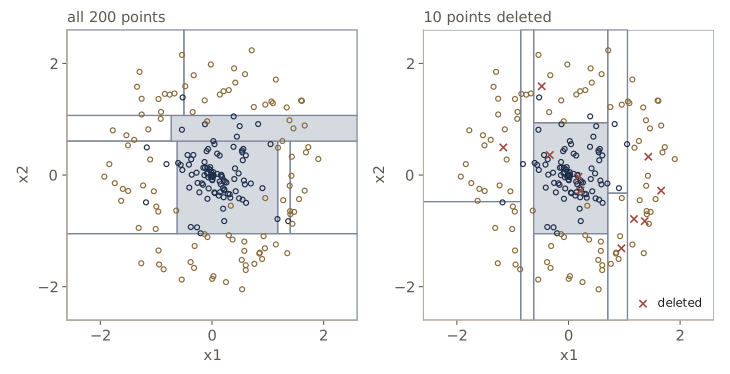
Watch out. Before drawing conclusions from the structure of one tree (“the model says temperature matters most”), regrow it on bootstrap samples and see whether the conclusion survives. Often it does not.
Limitations, and bagging trees
Instability is one of several weaknesses. The splits are aligned with the axes, so a boundary that runs diagonally needs a staircase of many splits where one oblique line would do:
rng_diag = np.random.default_rng(6)
X_diag = rng_diag.uniform(0, 1, (400, 2))
c_diag = (X_diag[:, 1] > X_diag[:, 0]).astype(int)      # class 1 above the diagonal
X_diag_test = rng_diag.uniform(0, 1, (4000, 2))
c_diag_test = (X_diag_test[:, 1] > X_diag_test[:, 0]).astype(int)
tree_diag = grow(X_diag, suff_stats(c_diag, "gini"), "gini", min_leaf=1)
test_err = np.mean(predict_tree(tree_diag, X_diag_test, "gini") != c_diag_test)
print(f"pure tree for the boundary x2 = x1: {n_leaves(tree_diag)} leaves, "
      f"test error {test_err:.4f}")
pure tree for the boundary x2 = x1: 18 leaves, test error 0.0635
Eighteen leaves, and still about 6% of test points on the wrong side, for a boundary that a single oblique split would get exactly right. The splits are also hard: each input belongs to exactly one leaf, so a regression tree is piecewise constant and jumps at every threshold, which is a poor fit to a smooth function.
Averaging addresses the instability and the jumps at once. Instability is high variance, and variance is what bagging removes. We bag 100 unpruned regression trees on the sine data and compare with the single trees:
rng_bt = np.random.default_rng(8)
single_pruned, _ = prune(big_tree, 0.5)
preds = []
for b in range(100):
    idx = rng_bt.integers(0, len(x_reg), len(x_reg))
    tree_b = grow(X_reg[idx], suff_stats(t_reg[idx], "sse"), "sse", min_leaf=2)
    preds.append(predict_tree(tree_b, X_grid, "sse"))
preds = np.array(preds)
for name, y in [("single unpruned tree", predict_tree(big_tree, X_grid, "sse")),
                ("single pruned tree  ", predict_tree(single_pruned, X_grid, "sse")),
                ("bagged trees, M=100 ", preds.mean(axis=0))]:
    print(f"{name}: error vs h {np.mean((y - h(x_grid))**2):.4f}")
print(f"bagged members: E_AV = {np.mean((preds - h(x_grid))**2):.4f}")
single unpruned tree: error vs h 0.0445
single pruned tree  : error vs h 0.0241
bagged trees, M=100 : error vs h 0.0214
bagged members: E_AV = 0.0572
Bagging more than halves the error of the unpruned tree, and it even edges out the pruned tree, whose \(\lambda\) was chosen with 100 extra validation points that the bagged trees never saw. Compare the polynomials, where bagging barely beat the single full-data model: a tree changes so much from one bootstrap sample to the next that its bootstrap copies disagree a lot, and the ambiguity term \(E_{\mathrm{AV}} - E_{\mathrm{COM}}\) removes much of the error. The price is the readability: a hundred trees do not tell a story. Random forests push the idea further by also choosing each split from a random subset of the input variables, which decorrelates the trees and so, by the \(\rho + (1 - \rho)/M\) formula, lowers the floor that averaging can reach. Boosted trees combine the trees of this section with the boosting of the last one. Both are among the strongest off-the-shelf methods for tabular data.
Conditional mixture models
Decision trees make hard, axis-aligned splits and put a constant in each region. We can relax all three choices at the cost of some readability: let the splits be soft and probabilistic, let them depend on all inputs at once, and let each region hold a probabilistic model. Carried to the end, this gives the hierarchical mixture of experts. We get there from the other direction, starting from the mixtures of module 09 and replacing each component density \(p(\mathbf{x} \mid k)\) by a conditional density \(p(t \mid \mathbf{x}, k)\).
Mixtures of linear regression models
Consider \(K\) linear regression models, each with its own weight vector \(\mathbf{w}_k\) and a shared noise precision \(\beta\), mixed with constant coefficients \(\pi_k\):
\[p(t \mid \boldsymbol{\theta}) = \sum_{k=1}^{K} \pi_k\, \mathcal{N}\!\left(t \mid \mathbf{w}_k^{\mathrm{T}} \boldsymbol{\phi}, \beta^{-1}\right),\]where \(\boldsymbol{\phi} = \boldsymbol{\phi}(\mathbf{x})\) is the basis-function vector of module 03 and \(\boldsymbol{\theta} = \{\mathbf{W}, \boldsymbol{\pi}, \beta\}\) collects the parameters. For data \(\{\boldsymbol{\phi}_n, t_n\}\) the log likelihood is
\[\ln p(\mathbf{t} \mid \boldsymbol{\theta}) = \sum_{n=1}^{N} \ln\left( \sum_{k=1}^{K} \pi_k\, \mathcal{N}\!\left(t_n \mid \mathbf{w}_k^{\mathrm{T}} \boldsymbol{\phi}_n, \beta^{-1}\right) \right).\]The sum inside the log blocks a closed-form maximum, exactly as for the Gaussian mixture, and the cure is the same: EM. Introduce a 1-of-\(K\) latent vector \(\mathbf{z}_n\) that says which line generated point \(n\). In the language of module 08, \(\mathbf{z}_n\) and \(\boldsymbol{\phi}_n\) are parents of \(t_n\), inside a plate over \(n\), with \(\boldsymbol{\pi}\), \(\mathbf{W}\) and \(\beta\) outside. If we knew \(\mathbf{Z}\), the log likelihood would split into separate pieces:
\[\ln p(\mathbf{t}, \mathbf{Z} \mid \boldsymbol{\theta}) = \sum_{n=1}^{N} \sum_{k=1}^{K} z_{nk} \left\{ \ln \pi_k + \ln \mathcal{N}\!\left(t_n \mid \mathbf{w}_k^{\mathrm{T}} \boldsymbol{\phi}_n, \beta^{-1}\right) \right\}.\]E step. With the current parameters, compute the posterior probability, or responsibility, of line \(k\) for point \(n\) by Bayes’ theorem:
\[\gamma_{nk} = \mathbb{E}[z_{nk}] = \frac{\pi_k\, \mathcal{N}\!\left(t_n \mid \mathbf{w}_k^{\mathrm{T}} \boldsymbol{\phi}_n, \beta^{-1}\right)}{\sum_{j} \pi_j\, \mathcal{N}\!\left(t_n \mid \mathbf{w}_j^{\mathrm{T}} \boldsymbol{\phi}_n, \beta^{-1}\right)}.\]M step. Maximize the expected complete-data log likelihood,
\[Q(\boldsymbol{\theta}, \boldsymbol{\theta}^{\text{old}}) = \sum_{n=1}^{N} \sum_{k=1}^{K} \gamma_{nk} \left\{ \ln \pi_k + \frac12 \ln \beta - \frac{\beta}{2} \left(t_n - \mathbf{w}_k^{\mathrm{T}} \boldsymbol{\phi}_n\right)^2 \right\} + \text{const},\]with the \(\gamma_{nk}\) held fixed. It separates into three problems, one for each kind of parameter.
Mixing coefficients. Maximize \(\sum_{n,k} \gamma_{nk} \ln \pi_k\) subject to \(\sum_k \pi_k = 1\). With a Lagrange multiplier, as for the Gaussian mixture, \(\pi_k = \frac{1}{N} \sum_n \gamma_{nk}\).
Weights. Only the squared errors involve \(\mathbf{w}_k\), each point weighted by \(\gamma_{nk}\). Setting the gradient to zero, \(\sum_n \gamma_{nk} (t_n - \mathbf{w}_k^{\mathrm{T}} \boldsymbol{\phi}_n) \boldsymbol{\phi}_n = \mathbf{0}\), or with \(\mathbf{R}_k = \operatorname{diag}(\gamma_{1k}, \dots, \gamma_{Nk})\) and the design matrix \(\mathbf{\Phi}\),
\[\mathbf{\Phi}^{\mathrm{T}} \mathbf{R}_k \left(\mathbf{t} - \mathbf{\Phi} \mathbf{w}_k\right) = \mathbf{0} \quad\Longrightarrow\quad \mathbf{w}_k = \left(\mathbf{\Phi}^{\mathrm{T}} \mathbf{R}_k \mathbf{\Phi}\right)^{-1} \mathbf{\Phi}^{\mathrm{T}} \mathbf{R}_k \mathbf{t}.\]Each line is fitted to all the data by weighted least squares, each point counting in proportion to how much that line is responsible for it. These are the same weighted normal equations as in the IRLS algorithm for logistic regression (module 04).
Precision. Setting the derivative with respect to \(\beta\) to zero, \(\sum_{n,k} \gamma_{nk} \{ \frac{1}{2\beta} - \frac12 (t_n - \mathbf{w}_k^{\mathrm{T}} \boldsymbol{\phi}_n)^2 \} = 0\), and using \(\sum_{n,k} \gamma_{nk} = N\),
\[\frac{1}{\beta} = \frac{1}{N} \sum_{n=1}^{N} \sum_{k=1}^{K} \gamma_{nk} \left(t_n - \mathbf{w}_k^{\mathrm{T}} \boldsymbol{\phi}_n\right)^2 .\]Our data come from two crossing lines, \(t = 0.9x + 0.4\) and \(t = -1.1x - 0.2\), with noise standard deviation 0.12. Which line a point uses depends on \(x\): the first line is more likely on the left, with probability \(\sigma(-5x)\). We will need that detail later; the constant-\(\pi\) mixture cannot see it.
rng_lin = np.random.default_rng(5)
N_lin = 200
x_lin = rng_lin.uniform(-1, 1, N_lin)
first = rng_lin.random(N_lin) < expit(-5 * x_lin)
t_lin = (np.where(first, 0.9 * x_lin + 0.4, -1.1 * x_lin - 0.2)
         + rng_lin.normal(0, 0.12, N_lin))
Phi_lin = np.c_[np.ones(N_lin), x_lin]           # phi(x) = (1, x)

def weighted_lstsq(Phi, t, g):
    """Solve Phi^T R (t - Phi w) = 0 with R = diag(g)."""
    return np.linalg.solve(Phi.T @ (g[:, None] * Phi), Phi.T @ (g * t))

def em_linear_mixture(Phi, t, K, rng, iters=100):
    """EM for a mixture of K linear regressions with shared precision beta."""
    N, M = Phi.shape
    W = rng.normal(0, 1, (K, M))
    pi, beta = np.full(K, 1.0 / K), 1.0 / np.var(t)
    history = []
    for it in range(iters):
        # E step: responsibilities, in log space
        log_p = np.log(pi) + log_gauss(t[:, None], Phi @ W.T, 1 / np.sqrt(beta))
        log_lik = logsumexp(log_p, axis=1)
        history.append(log_lik.sum())
        gamma = np.exp(log_p - log_lik[:, None])
        # M step
        pi = gamma.mean(axis=0)
        W = np.array([weighted_lstsq(Phi, t, gamma[:, k]) for k in range(K)])
        beta = N / np.sum(gamma * (t[:, None] - Phi @ W.T)**2)
    return W, pi, beta, gamma, np.array(history)

W_mix, pi_mix, beta_mix, gamma_mix, hist_mix = em_linear_mixture(
    Phi_lin, t_lin, 2, np.random.default_rng(0))
for it in [0, 1, 5, 10, 20, 99]:
    print(f"iteration {it:3d}: log likelihood {hist_mix[it]:9.3f}")
print("log likelihood never decreased:", bool(np.all(np.diff(hist_mix) >= -1e-9)))
for k in range(2):
    print(f"line {k + 1}: intercept {W_mix[k, 0]:.3f}  slope {W_mix[k, 1]:.3f}  "
          f"pi {pi_mix[k]:.3f}")
print(f"noise std 1/sqrt(beta) = {1 / np.sqrt(beta_mix):.4f}")
iteration   0: log likelihood  -289.212
iteration   1: log likelihood   -98.668
iteration   5: log likelihood    -2.860
iteration  10: log likelihood    20.819
iteration  20: log likelihood    20.874
iteration  99: log likelihood    20.874
log likelihood never decreased: True
line 1: intercept -0.209  slope -1.052  pi 0.528
line 2: intercept 0.401  slope 0.936  pi 0.472
noise std 1/sqrt(beta) = 0.1200
EM recovers both lines (in its own order: labels are arbitrary) and the noise level. The log likelihood rises at every iteration, as the EM theory of module 09 guarantees. Two quick checks: the weighted normal equations agree with ordinary least squares on rows scaled by \(\sqrt{\gamma_{nk}}\), and the mixture’s fit is far better than a single regression line’s.
g = gamma_mix[:, 0]
r = np.sqrt(g)
w_scaled = np.linalg.lstsq(r[:, None] * Phi_lin, r * t_lin, rcond=None)[0]
print("weighted normal equations match scaled lstsq:",
      np.allclose(w_scaled, weighted_lstsq(Phi_lin, t_lin, g)))

w_one = np.linalg.lstsq(Phi_lin, t_lin, rcond=None)[0]
beta_one = N_lin / np.sum((t_lin - Phi_lin @ w_one)**2)
ll_one = log_gauss(t_lin, Phi_lin @ w_one, 1 / np.sqrt(beta_one)).sum()
print(f"log likelihood: single line {ll_one:.3f}   two lines {hist_mix[-1]:.3f}")
weighted normal equations match scaled lstsq: True
log likelihood: single line -115.657   two lines 20.874
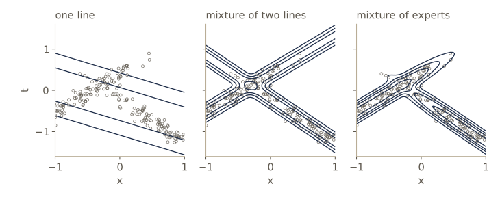
The middle panel shows the weakness of constant mixing coefficients. At \(x = -0.9\) almost every point lies on the first line, but the model still puts roughly half of its probability on the second. The mixture has learned what the two lines are, but not where each one applies. We fix this in the section on mixtures of experts.
Note. For squared loss, the best point prediction is the conditional mean, here \(\sum_k \pi_k \mathbf{w}_k^{\mathrm{T}} \boldsymbol{\phi}\), a line between the two. With bimodal data it runs where there are hardly any points. When the predictive distribution has several modes, report the distribution, or its modes, rather than its mean.
Mixtures of logistic models
The same recipe turns logistic regression into a mixture. With \(y_k = \sigma(\mathbf{w}_k^{\mathrm{T}} \boldsymbol{\phi})\) and \(t \in \{0, 1\}\),
\[p(t \mid \boldsymbol{\phi}, \boldsymbol{\theta}) = \sum_{k=1}^{K} \pi_k\, y_k^{t} \left[1 - y_k\right]^{1 - t}.\]The E step computes \(\gamma_{nk} \propto \pi_k\, y_{nk}^{t_n} [1 - y_{nk}]^{1 - t_n}\) with \(y_{nk} = \sigma(\mathbf{w}_k^{\mathrm{T}} \boldsymbol{\phi}_n)\). In the M step, \(\pi_k\) is again the average responsibility, and each \(\mathbf{w}_k\) maximizes \(\sum_n \gamma_{nk} \{ t_n \ln y_{nk} + (1 - t_n) \ln(1 - y_{nk}) \}\), a logistic regression in which point \(n\) carries weight \(\gamma_{nk}\). That has no closed form, but its gradient and Hessian,
\[\nabla_{\mathbf{w}_k} = \sum_{n=1}^{N} \gamma_{nk} (t_n - y_{nk}) \boldsymbol{\phi}_n, \qquad \mathbf{H}_k = -\sum_{n=1}^{N} \gamma_{nk}\, y_{nk}(1 - y_{nk})\, \boldsymbol{\phi}_n \boldsymbol{\phi}_n^{\mathrm{T}},\]are those of module 04 with weights attached, so a few IRLS (Newton) steps do the job. The components interact only through the responsibilities, so the \(K\) weight vectors are updated separately. Doing only a few Newton steps per M step, rather than maximizing fully, is a generalized EM algorithm: each M step increases \(Q\) without maximizing it, which is enough to keep the likelihood from falling.
A mixture helps when the population is made of groups that respond differently. In our example, 60% of the cases become more likely to have \(t = 1\) as \(x\) grows and 40% less likely, so the overall probability is U-shaped in \(x\), which a single logistic curve (always monotone) cannot follow.
rng_lg = np.random.default_rng(7)
N_lg = 800
x_lg = rng_lg.uniform(-3, 3, N_lg)
group = rng_lg.random(N_lg) < 0.6
a_lg = np.where(group, 3 * (x_lg - 0.5), -3 * (x_lg + 0.5))   # each group's activation
t_lg = (rng_lg.random(N_lg) < expit(a_lg)).astype(float)
Phi_lg = np.c_[np.ones(N_lg), x_lg]

def log_bernoulli(t, a):
    """ln sigma(a)^t (1 - sigma(a))^(1 - t), computed stably from the activation a."""
    return -t * np.logaddexp(0, -a) - (1 - t) * np.logaddexp(0, a)

def irls(Phi, t, g, w, steps, alpha=1e-2):
    """Newton steps for logistic regression, point weights g, prior precision alpha."""
    for _ in range(steps):
        y = expit(Phi @ w)
        H = Phi.T @ ((g * y * (1 - y))[:, None] * Phi) + alpha * np.eye(len(w))
        w = w + np.linalg.solve(H, Phi.T @ (g * (t - y)) - alpha * w)
    return w

def em_logistic_mixture(Phi, t, K, rng, iters=150):
    N, M = Phi.shape
    W, pi, history = rng.normal(0, 1, (K, M)), np.full(K, 1.0 / K), []
    for it in range(iters):
        log_p = np.log(pi) + log_bernoulli(t[:, None], Phi @ W.T)
        log_lik = logsumexp(log_p, axis=1)
        history.append(log_lik.sum())
        gamma = np.exp(log_p - log_lik[:, None])
        pi = gamma.mean(axis=0)
        W = np.array([irls(Phi, t, gamma[:, k], W[k], steps=2) for k in range(K)])
    return W, pi, np.array(history)

w_lg1 = irls(Phi_lg, t_lg, np.ones(N_lg), np.zeros(2), steps=25)
W_lg, pi_lg, hist_lg = em_logistic_mixture(Phi_lg, t_lg, 2, np.random.default_rng(0))
ll_single = log_bernoulli(t_lg, Phi_lg @ w_lg1).sum()
print(f"log likelihood: single logistic {ll_single:.2f}   mixture {hist_lg[-1]:.2f}")
xs = np.array([-2.5, -1.0, 0.0, 1.0, 2.5]); Ps = np.c_[np.ones(5), xs]
print("x:              ", xs)
print("true p(t=1|x):  ", 0.6 * expit(3 * (xs - 0.5)) + 0.4 * expit(-3 * (xs + 0.5)))
print("single logistic:", expit(Ps @ w_lg1))
print("mixture of two: ", expit(Ps @ W_lg.T) @ pi_lg)
log likelihood: single logistic -530.18   mixture -511.04
x:               [-2.5 -1.   0.   1.   2.5]
true p(t=1|x):   [0.3991 0.3336 0.1824 0.4949 0.5986]
single logistic: [0.2973 0.3584 0.402  0.4472 0.5165]
mixture of two:  [0.3961 0.3008 0.2338 0.4232 0.5826]
The single logistic model can only tilt one way, so it misses the high probability on the left. The mixture follows the U shape. (The small prior precision \(\alpha\) in irls keeps a weight vector from running off to infinity when a component’s weighted data happen to be separable, the problem we met in module 04.) Binary targets carry little information per point, so different runs of EM can land on somewhat different weight vectors that give almost the same \(p(t \mid x)\); judge the fit by its predictions, not by its parameters.
Mixtures of experts
Back to the two-line example, where the constant mixing coefficients were the problem. Let them depend on the input:
\[p(t \mid \mathbf{x}) = \sum_{k=1}^{K} \pi_k(\mathbf{x})\, p_k(t \mid \mathbf{x}).\]This is a mixture of experts. The components \(p_k(t \mid \mathbf{x})\) are the experts, and the mixing coefficients \(\pi_k(\mathbf{x})\) are the gating functions, which decide which expert to trust where. They must be nonnegative and sum to one at every \(\mathbf{x}\), so a natural choice is a softmax of linear functions, \(\pi_k(\mathbf{x}) = \exp(\mathbf{v}_k^{\mathrm{T}} \boldsymbol{\phi}) / \sum_j \exp(\mathbf{v}_j^{\mathrm{T}} \boldsymbol{\phi})\), the multiclass logistic model of module 04. For \(K = 2\) this is \(\pi_1(\mathbf{x}) = \sigma(\mathbf{v}^{\mathrm{T}} \boldsymbol{\phi})\).
EM goes through almost unchanged. The E step uses \(\pi_k(\mathbf{x}_n)\) in place of \(\pi_k\). In the M step the experts are updated exactly as before (weighted least squares for linear-Gaussian experts), and the gate maximizes
\[\sum_{n=1}^{N} \sum_{k=1}^{K} \gamma_{nk} \ln \pi_k(\mathbf{x}_n),\]which is the cross-entropy of a logistic (or softmax) regression whose targets are the soft labels \(\gamma_{nk}\) instead of 0/1 labels. The gradient keeps its familiar form, \(\sum_n (\gamma_{n1} - \pi_1(\mathbf{x}_n)) \boldsymbol{\phi}_n\) for \(K = 2\), and the problem is concave, so IRLS applies. Every M step is a convex problem, even though the likelihood as a whole is not concave and EM finds a local maximum.
def em_experts(Phi, t, rng, iters=100, newton_steps=3):
    """Two linear-Gaussian experts with a logistic gate pi_1(x) = sigma(v^T phi)."""
    N, M = Phi.shape
    W, v, beta = rng.normal(0, 1, (2, M)), np.zeros(M), 1.0 / np.var(t)
    history = []
    for it in range(iters):
        a = Phi @ v
        log_gate = np.c_[-np.logaddexp(0, -a), -np.logaddexp(0, a)]   # ln pi_1, ln pi_2
        log_p = log_gate + log_gauss(t[:, None], Phi @ W.T, 1 / np.sqrt(beta))
        log_lik = logsumexp(log_p, axis=1)
        history.append(log_lik.sum())
        gamma = np.exp(log_p - log_lik[:, None])
        W = np.array([weighted_lstsq(Phi, t, gamma[:, k]) for k in range(2)])
        beta = N / np.sum(gamma * (t[:, None] - Phi @ W.T)**2)
        for _ in range(newton_steps):         # gate: logistic regression, soft targets
            y = expit(Phi @ v)
            H = Phi.T @ ((y * (1 - y))[:, None] * Phi) + 1e-6 * np.eye(M)
            v = v + np.linalg.solve(H, Phi.T @ (gamma[:, 0] - y))
    return W, v, beta, np.array(history)

W_moe, v_moe, beta_moe, hist_moe = em_experts(Phi_lin, t_lin, np.random.default_rng(0))
print("log likelihood never decreased:", bool(np.all(np.diff(hist_moe) >= -1e-9)))
print(f"log likelihood: single line {ll_one:.2f}   mixture {hist_mix[-1]:.2f}   "
      f"mixture of experts {hist_moe[-1]:.2f}")
for k in range(2):
    print(f"expert {k + 1}: intercept {W_moe[k, 0]:.3f}  slope {W_moe[k, 1]:.3f}")
print(f"gate: pi_1(x) = sigma({v_moe[0]:.2f} + {v_moe[1]:.2f} x)")
for x0 in [-0.9, 0.0, 0.9]:
    k1 = np.argmax(W_mix[:, 1])             # the mixture's line with positive slope
    k2 = np.argmax(W_moe[:, 1])             # the expert with positive slope
    gate = expit(v_moe[0] + v_moe[1] * x0)
    print(f"x = {x0:4.1f}: weight on the rising line: mixture {pi_mix[k1]:.3f}   "
          f"experts {gate if k2 == 0 else 1 - gate:.3f}")
log likelihood never decreased: True
log likelihood: single line -115.66   mixture 20.87   mixture of experts 91.82
expert 1: intercept -0.206  slope -1.059
expert 2: intercept 0.401  slope 0.934
gate: pi_1(x) = sigma(-0.02 + 5.40 x)
x = -0.9: weight on the rising line: mixture 0.472   experts 0.992
x =  0.0: weight on the rising line: mixture 0.472   experts 0.505
x =  0.9: weight on the rising line: mixture 0.472   experts 0.008
The experts are the same two lines, but now the gate has learned where each applies: the rising line gets nearly all the weight on the left, nearly none on the right, and they share near the crossing. The log likelihood improves from 20.87 to 91.82, and the right panel of the figure shows the predictive density fading out where a line has no data. (The data were generated with a gate of \(\sigma(-5x)\) on the rising line; the fitted gate, \(1 - \sigma(-0.02 + 5.40x) = \sigma(0.02 - 5.40x)\), is close to it.)
Hierarchical mixtures of experts
A mixture of experts with linear gates and linear experts is still limited: one linear gate can only divide the input space into two soft half-spaces. More flexible models come from nesting. In a hierarchical mixture of experts (HME) each component of the top-level mixture is itself a mixture of experts, with its own gate:
\[p(t \mid \mathbf{x}) = \sum_{k} \pi_k(\mathbf{x}) \sum_{j} \pi_{j \mid k}(\mathbf{x})\, p_{kj}(t \mid \mathbf{x}).\]With constant mixing coefficients the nesting would add nothing: multiply out and it is a flat mixture with coefficients \(\pi_k \pi_{j \mid k}\). With input-dependent linear gates it does add something, because the product of two logistic functions is not in general a softmax of linear functions. The flat model cannot always imitate the nested one (Bishop exercise 14.17 asks for a counterexample).
Read as a tree, the HME is a soft, probabilistic decision tree. Each gate is an internal node that sends the input left and right with probabilities rather than a hard yes or no, the split is along any direction \(\mathbf{v}^{\mathrm{T}} \boldsymbol{\phi}\) rather than one axis, and each leaf holds a probabilistic model (a regression line or a classifier) rather than a constant. It is fitted by EM with IRLS for the gates and experts in the M step. A Bayesian version using the variational methods of module 10 also exists (Bishop §14.5.3 has the reference).
Compare the mixture density network of module 05, which also outputs input-dependent mixing coefficients and component parameters, but computes all of them from shared hidden units of one neural network. The trade-off is between the two ways of fitting. The mixture of experts is trained by EM, and every M step is a convex problem. The mixture density network is trained by gradient descent on a nonconvex error, but its components share features, and its soft splits can be curved, not only oblique.
Looking back over the course
This module has been about combining models, and in a sense the whole course has too. The same few ideas came back again and again, in different combinations.
| Idea | Where we met it | Where it appeared here |
|---|---|---|
| Likelihoods: write down \(p(\text{data} \mid \text{parameters})\) and maximize it | least squares as Gaussian likelihood (03), cross-entropy for classification (04, 05), mixtures (09), hidden Markov models (13) | mixtures of regressions, logistic models, and experts; cross-entropy versus exponential error |
| Priors: put a distribution on the parameters and reason with the posterior | Bayesian linear regression and the evidence (03), weight decay as a Gaussian prior (01, 05), Gaussian processes (06), relevance vector machines (07) | Bayesian model averaging; the small prior in IRLS that tames separable data |
| Latent variables: explain data through unobserved causes and fit with EM | Gaussian mixtures (09), probabilistic PCA and factor analysis (12), hidden Markov and linear dynamical systems (13) | the component label \(z_n\) of every conditional mixture |
| Approximations: when the exact computation is out of reach, approximate it with care | Laplace (04), variational inference and expectation propagation (10), Monte Carlo (11), EM’s lower bound (09) | stagewise fitting in boosting; greedy tree growing; generalized EM with a few Newton steps |
Graphical models (module 08) gave all of these a common language: a picture of which variables depend on which, and message-passing algorithms that exploit it. And decision theory (module 01) separated what we believe, a posterior or a predictive distribution, from what we do with it, a class decision or a point prediction.
Where to go next. The largest development in machine learning since our course text appeared in 2006 is deep learning: the networks of module 05, made much deeper, trained on much more data with better optimizers and architectures (convolutional networks for images, recurrent and attention-based networks for sequences), and used as the flexible pieces inside probabilistic models. Almost everything in this course carries over. Training minimizes a negative log likelihood; regularization is a prior in disguise; a variational autoencoder is a nonlinear cousin of the latent-variable models of module 12, fitted with the variational bound of module 10; a network with a softmax output is the classifier of module 04 on learned features; and ensembles of networks are committees. Jue’s CSE 676 Deep Learning course picks up from here, and the EAS 510 notes are a hands-on introduction to PyTorch if you want to start building networks right away.
Summary
| Method | Members | How they are combined | How it is fitted |
|---|---|---|---|
| Bayesian model averaging | complete rival models \(h\) | posterior weights \(p(h \mid \mathbf{X})\), one model for the whole data set | Bayes’ theorem with the evidence \(p(\mathbf{X} \mid h)\) |
| Bagging | same model on bootstrap data sets | plain average (or majority vote) | each member independently |
| AdaBoost | weak learners (e.g. stumps) on reweighted data | weighted vote with \(\alpha_m = \ln\{(1 - \epsilon_m)/\epsilon_m\}\) | stagewise minimization of \(\sum_n e^{-t_n f(\mathbf{x}_n)}\) |
| Decision tree (CART) | a constant per axis-aligned box | the input selects exactly one leaf | greedy splits by squared error, Gini, or cross-entropy; cost-complexity pruning |
| Mixture of linear / logistic models | \(K\) regression or classification models | constant mixing coefficients \(\pi_k\) | EM: responsibilities, then weighted least squares or weighted IRLS |
| Mixture of experts, HME | experts \(p_k(t \mid \mathbf{x})\) | gating functions \(\pi_k(\mathbf{x})\), possibly nested | EM with a soft-target logistic regression for each gate |
Ideas to carry forward:
- Averaging reduces variance, never bias, and only the uncorrelated part of the members’ errors: \(E_{\mathrm{COM}} = \sigma^2(\rho + (1 - \rho)/M)\). A committee is never worse than its average member, and it gains exactly as much as its members disagree.
- Boosting is stagewise fitting of an additive model. The exponential error gives AdaBoost’s simple reweighting, estimates half the log odds, and is harsh on outliers; other errors give other boosting algorithms.
- Trees are readable and fast but unstable, axis-aligned, and piecewise constant. Averaging many of them (bagging, random forests, boosted trees) trades readability for accuracy.
- Letting the input choose the model, softly, turns mixtures into mixtures of experts: probabilistic decision trees that EM can fit.
Exercises
- A committee may weight its members unequally, \(y_{\mathrm{COM}} = \sum_m \alpha_m y_m\) with \(\alpha_m \ge 0\) and \(\sum_m \alpha_m = 1\). Show that its expected squared error is at most \(\sum_m \alpha_m \mathbb{E}_{\mathbf{x}}[\epsilon_m^2]\), and write the gap as a weighted spread of the members around \(y_{\mathrm{COM}}\). Then show that the same inequality holds for any error \(E(y)\) that is convex in \(y\).
- For members with equal error \(\sigma^2\) and pairwise correlation \(\rho\), how large must \(M\) be for the committee’s error to come within 10% of its limit \(\rho \sigma^2\)? Evaluate for \(\rho = 0.1\) and \(\rho = 0.5\), and confirm with
committee_errors. - Show that the probability that a given point is missing from a bootstrap data set is \((1 - 1/N)^N\) and that it tends to \(e^{-1}\). Then compute the out-of-bag error of the bagged polynomial committee: predict each of the 25 training points with only the members whose bootstrap set left it out, and compare the resulting mean squared error with the committee’s true error.
- Prove that right after AdaBoost’s reweighting step, the member just added has a weighted error rate of exactly \(1/2\) under the new weights, so the next stump cannot be the same one. Check it numerically on the ring data with
W_hist. - Use the result \(y^\star = \tfrac12 \ln\{p(t{=}1 \mid \mathbf{x}) / p(t{=}{-1} \mid \mathbf{x})\}\) to turn the AdaBoost score into a probability, \(\sigma(2 f_m(\mathbf{x}))\). For the ring data, compute the true class posterior (from the two radial densities) at the test points and compare it with the boosted estimate after 10 and after 300 rounds. Which one is better calibrated, and why?
- Suppose we tried to read the exponential error as a negative log likelihood, \(p(t \mid \mathbf{x}) \propto \exp(-e^{-t y(\mathbf{x})})\) with no further normalization. Show that \(p(t{=}1 \mid \mathbf{x}) + p(t{=}{-1} \mid \mathbf{x}) = 1\) holds only for special values of \(y\), so the exponential error is not the log likelihood of a normalized model.
- Implement gradient boosting for classification with the cross-entropy error \(\ln(1 + e^{-t f})\): at each round, fit a least-squares regression stump (in either variable) to the negative gradient \(t_n \sigma(-t_n f(\mathbf{x}_n))\) and add it with a shrinkage factor. Repeat the flipped-label experiment and compare how much influence the 10 flipped points gain with what happened under AdaBoost.
- Show that the Gini index \(\sum_k p_k(1 - p_k)\) and the cross-entropy \(-\sum_k p_k \ln p_k\) are strictly concave functions of \((p_1, \dots, p_K)\) on the probability simplex. Use this to prove that any split of a node into two children with different class proportions strictly lowers the size-weighted Gini index, while it may leave the misclassification count unchanged. Give an example with three classes.
- Replace the single validation set in the pruning experiment by 5-fold cross-validation: for each fold, grow a full tree on the other four folds, prune it for each \(\lambda\) in a grid, and record the held-out error. Pick \(\lambda\) and compare the chosen tree size with the one the validation set picked.
- For the mixture of two linear regressions fitted above, compute the conditional mean \(\mathbb{E}[t \mid x] = \sum_k \pi_k \mathbf{w}_k^{\mathrm{T}} \boldsymbol{\phi}(x)\), and the conditional mean of the mixture of experts. Plot both against the data. Which is a sensible point prediction, and at which values of \(x\) does each fail?
- Extend
em_expertsto \(K\) experts with a softmax gate: in the M step, fit the gate by a few Newton steps of multiclass logistic regression with soft targets \(\gamma_{nk}\). Generate data from three line segments that take over from each other as \(x\) increases, fit \(K = 3\), and report the log likelihood and the learned gate at a few values of \(x\). - In your own words: explain to a classmate the difference between bagging, boosting, and a mixture of experts. For each one, say what makes the members different from each other, how their outputs are combined, and what kind of error (bias or variance) the combination mainly reduces.
Going further
- Bishop, Pattern Recognition and Machine Learning, chapter 14 — the source for this module. Exercises 14.2–14.4 cover committee errors, 14.6–14.7 the AdaBoost coefficient and the minimizer of the exponential error, 14.9 boosting with squared error, 14.11 impurity measures, 14.13–14.15 the mixture of linear regressions, and 14.17 the hierarchical mixture of experts.
- Trevor Hastie, Robert Tibshirani, and Jerome Friedman, The Elements of Statistical Learning, 2nd edition (free PDF from the authors) — chapter 8.7 (bagging), 9.2 (trees) and 9.5 (hierarchical mixtures of experts), chapter 10 (boosting and boosted trees), and chapter 15 (random forests), with many experiments.
- Leo Breiman, “Bagging predictors”, Machine Learning, 1996 — the paper that introduced bagging, with a discussion of why unstable procedures benefit most.
- Yoav Freund and Robert E. Schapire, “A decision-theoretic generalization of on-line learning and an application to boosting”, Journal of Computer and System Sciences, 1997; and Jerome Friedman, Trevor Hastie, and Robert Tibshirani, “Additive logistic regression: a statistical view of boosting”, Annals of Statistics, 2000 — AdaBoost, and its reinterpretation as stagewise minimization of the exponential error.
- Michael I. Jordan and Robert A. Jacobs, “Hierarchical mixtures of experts and the EM algorithm”, Neural Computation, 1994 — the HME model and its EM training.
- Christopher M. Bishop and Hugh Bishop, Deep Learning: Foundations and Concepts (Springer, 2024) — a natural next book after this course, written in the same notation and style as our text.
These notes follow the chapters of C. M. Bishop, Pattern Recognition and Machine Learning (Springer, 2006), the course text, which Microsoft Research makes freely available as a PDF. The explanations, code, figures, and exercises here are written for this course; the book remains the reference, with the full derivations and many more exercises.