CSE 676 · Module 14 · Week 11
Sampling
Monte Carlo estimates, transformation, rejection and importance sampling, Markov chain Monte Carlo (Metropolis–Hastings and Gibbs), and Langevin sampling for training energy-based models.
Companion reading: Bishop & Bishop, Deep Learning: Foundations and Concepts, chapter 14, “Sampling”
By the end of this module you can
- Estimate an expectation by Monte Carlo, show that the estimator is unbiased with variance \(\operatorname{var}[f]/L\), and measure the \(1/\sqrt{L}\) error in one and in a hundred dimensions.
- Turn uniform random numbers into exponential, Cauchy, Gaussian, and correlated Gaussian samples with the inverse-CDF method, the Box–Muller method, and a Cholesky factor.
- Implement rejection sampling and a simple adaptive rejection sampler, predict the acceptance rate from the envelope, and explain why it decays exponentially with dimension.
- Use importance sampling and sampling-importance-resampling with unnormalized densities, compute the effective sample size, and show how it collapses as the proposal and the target drift apart or the dimension grows.
- State invariance, detailed balance, and ergodicity for a Markov chain, and verify them on a small discrete chain through its eigenvectors.
- Implement Metropolis–Hastings and Gibbs sampling, measure acceptance rates and autocorrelation times, and explain the proposal-scale trade-off and why Gibbs sampling mixes slowly under strong correlation.
- Derive the positive-phase and negative-phase gradient of an energy-based model’s log-likelihood and check it against quadrature.
- Sample from a known density with Langevin dynamics, quantify the bias of a finite step size, and train a small energy network in PyTorch with short-run Langevin negatives.
Contents
- Basic sampling algorithms
- Markov chain Monte Carlo
- Langevin sampling
- Summary
- Exercises
- Going further
Randomness runs through deep learning. A minibatch gradient is a Monte Carlo estimate of the full gradient (module 07); dropout samples a sub-network at every step (module 09); and every generative model in the second half of the course is judged, in the end, by the samples it produces. Some of those samples are easy to get. A directed graphical model is sampled one node at a time, parents first (module 11), and a latent-variable model by drawing a latent vector and running a network forward (module 16). Others are hard: the posterior over latent variables, or a density that we can evaluate only up to an unknown normalizing constant.
This module collects the sampling tools the rest of the course relies on. We start from uniform random numbers and build samplers for standard distributions, then look at rejection sampling and importance sampling, which work well in one or two dimensions and fail in many. Markov chain Monte Carlo (MCMC) trades independence for scalability: the samples form a chain whose long-run distribution is the one we want. Finally, Langevin dynamics uses the gradient of the log density to move samples uphill, which is exactly what we need to train and sample from energy-based models, and which leads directly to the score-based diffusion models of module 20.
Much of the first two sections also appears in Intro to ML, module 11, which goes further into slice sampling, Hamiltonian Monte Carlo, and estimating partition functions. Here we keep the classical material compact, measure every claim with NumPy, and spend the extra space on energy-based models, the part of the story that belongs to deep learning.
import numpy as np
import torch
from scipy.special import logsumexp, ndtr, digamma, polygamma

np.set_printoptions(precision=4, suppress=True)
rng = np.random.default_rng(14)
torch.manual_seed(14)
Basic sampling algorithms
Everything in this module starts from a supply of numbers that behave as if they were drawn independently and uniformly from \((0, 1)\). A computer produces them with a deterministic algorithm, so they are pseudo-random, but a good generator passes every statistical test we care about. NumPy’s default_rng is such a generator, and seeding it makes every result below repeatable.
Expectations
Often we do not need samples for their own sake. We need an expectation
\[\mathbb{E}[f] = \int f(\mathbf{z})\, p(\mathbf{z})\, \mathrm{d}\mathbf{z},\](a sum for discrete variables) that we cannot compute in closed form. If \(\mathbf{z}^{(1)}, \dots, \mathbf{z}^{(L)}\) are drawn independently from \(p(\mathbf{z})\), the Monte Carlo estimator
\[\widehat{f} = \frac{1}{L} \sum_{l=1}^{L} f(\mathbf{z}^{(l)})\]replaces the integral by an average. Each term has mean \(\mathbb{E}[f]\), so \(\mathbb{E}[\widehat{f}] = \mathbb{E}[f]\): the estimator is unbiased. The terms are independent, so their variances add, and dividing by \(L^2\) gives
Result. The Monte Carlo estimator has variance
\[\operatorname{var}[\widehat{f}] = \frac{1}{L}\, \mathbb{E}\left[ (f - \mathbb{E}[f])^2 \right],\]so its standard error falls as \(1/\sqrt{L}\), with a constant that is the standard deviation of \(f(\mathbf{z})\) under \(p\).
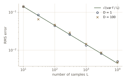
The dimension of \(\mathbf{z}\) appears nowhere in this formula. That is the great strength of Monte Carlo compared with numerical quadrature, whose grids grow exponentially with the dimension. Let us measure it. Take \(\mathbf{z} \sim \mathcal{N}(\mathbf{0}, \mathbf{I})\) in \(D\) dimensions and \(f(\mathbf{z}) = \cos(\mathbf{a}^{\mathrm{T}}\mathbf{z})\) for a unit vector \(\mathbf{a}\). Since \(\mathbf{a}^{\mathrm{T}}\mathbf{z}\) is a standard Gaussian whatever \(D\) is, \(\mathbb{E}[f] = e^{-1/2}\) and \(\operatorname{var}[f] = \tfrac12(1 + e^{-2}) - e^{-1} \approx 0.1998\) in every dimension.
def mc_rms_error(D, L, n_rep, rng):
    """RMS error of the Monte Carlo estimate of E[cos(a^T z)], z ~ N(0, I_D), over n_rep repeats."""
    a = rng.standard_normal(D)
    a /= np.linalg.norm(a)
    est = np.array([np.cos(rng.standard_normal((L, D)) @ a).mean() for _ in range(n_rep)])
    return np.sqrt(np.mean((est - np.exp(-0.5)) ** 2))

var_f = 0.5 * (1 + np.exp(-2)) - np.exp(-1)
print("    L    D = 1    D = 100   theory sqrt(var f / L)")
for L in [10, 100, 1000, 10000]:
    e1, e100 = mc_rms_error(1, L, 100, rng), mc_rms_error(100, L, 100, rng)
    print(f"{L:5d}   {e1:.4f}   {e100:.4f}    {np.sqrt(var_f / L):.4f}")
    L    D = 1    D = 100   theory sqrt(var f / L)
   10   0.1402   0.1744    0.1413
  100   0.0450   0.0465    0.0447
 1000   0.0144   0.0126    0.0141
10000   0.0046   0.0044    0.0045
The errors in one and a hundred dimensions both follow the formula, up to the scatter we should expect from only 100 repeats, and each factor of 100 in \(L\) buys one more decimal digit. Two caveats temper the good news. First, the formula assumes independent samples; the MCMC samples of the next section are correlated, and their error is larger. Second, the constant \(\operatorname{var}[f]\) can be enormous relative to \(\mathbb{E}[f]^2\). The classic case is a function that is large only where \(p\) is small, such as the probability of a rare event:
L = 10_000
z = rng.standard_normal(L)
print(f"P(z > 4): exact {ndtr(-4):.3e},  Monte Carlo with L = {L}: {np.mean(z > 4):.3e}")
P(z > 4): exact 3.167e-05, Monte Carlo with L = 10000: 0.000e+00
With ten thousand samples we expect a third of a sample beyond 4, so the estimate is usually exactly zero. Its relative error is about \(1/\sqrt{L\,P}\), which here asks for millions of samples. Importance sampling, below, fixes this example.
Standard distributions
Suppose \(z\) is uniform on \((0, 1)\) and we set \(y = g(z)\) for an increasing function \(g\). By the change-of-variables formula of module 02, \(p(y) = p(z)\, \lvert \mathrm{d}z / \mathrm{d}y \rvert = \mathrm{d}z/\mathrm{d}y\). We want this to equal a chosen density \(p(y)\), so \(z\) must be the cumulative distribution function of \(y\):
\[z = h(y) \equiv \int_{-\infty}^{y} p(\widehat{y})\, \mathrm{d}\widehat{y}, \qquad y = h^{-1}(z).\]This is the inverse-CDF method (also called the transformation method): feed uniform numbers through the inverse of the target’s cumulative distribution function. For the exponential density \(p(y) = \lambda e^{-\lambda y}\) on \(y \geq 0\), \(h(y) = 1 - e^{-\lambda y}\) and \(y = -\lambda^{-1} \ln(1 - z)\). For the standard Cauchy density \(p(y) = 1/\{\pi(1 + y^2)\}\), \(h(y) = \tfrac12 + \pi^{-1}\arctan y\) and \(y = \tan\{\pi(z - \tfrac12)\}\).
def sample_exponential(lam, L, rng):
    return -np.log1p(-rng.random(L)) / lam          # y = h^{-1}(z) with h(y) = 1 - exp(-lam y)

def sample_cauchy(L, rng):
    return np.tan(np.pi * (rng.random(L) - 0.5))     # y = tan(pi (z - 1/2))

y = sample_exponential(2.5, 200_000, rng)
print(f"exponential, lambda = 2.5: mean {y.mean():.4f} (exact 0.4),"
      f"  var {y.var():.4f} (exact 0.16)")
y = sample_cauchy(200_000, rng)
print("Cauchy quartiles:", np.quantile(y, [0.25, 0.5, 0.75]), "(exact -1, 0, 1)")
exponential, lambda = 2.5: mean 0.3990 (exact 0.4),  var 0.1593 (exact 0.16)
Cauchy quartiles: [-0.9988 -0.0001  1.007 ] (exact -1, 0, 1)
For the Cauchy we check quantiles rather than moments, because its mean and variance do not exist: the sample mean of Cauchy draws never settles down however large \(L\) is.
The Gaussian has no closed-form inverse CDF, but in two dimensions it does have a closed-form description in polar coordinates, and that gives the Box–Muller method. Draw pairs \((z_1, z_2)\) uniformly in the square \((-1, 1)^2\) and keep only those inside the unit disk, so that the kept points are uniform in the disk. Set \(r^2 = z_1^2 + z_2^2\) and
\[y_1 = z_1 \left( \frac{-2 \ln r^2}{r^2} \right)^{1/2}, \qquad y_2 = z_2 \left( \frac{-2 \ln r^2}{r^2} \right)^{1/2}.\]Why this works: a point uniform in the disk has an angle \(\theta\) uniform on \([0, 2\pi)\) and, independently, \(r^2\) uniform on \((0, 1)\) (the area inside radius \(r\) is proportional to \(r^2\)). The map keeps the angle and sends the squared radius to \(R^2 = y_1^2 + y_2^2 = -2 \ln r^2\), which by the exponential example (with \(1 - z\) replaced by the equally uniform \(r^2\)) is exponential with mean 2. A standard two-dimensional Gaussian has exactly this polar description: a uniform angle and, independently, an exponential squared radius with mean 2, because its density \(\tfrac{1}{2\pi} e^{-R^2/2}\) depends only on \(R\). So \(y_1\) and \(y_2\) are independent standard Gaussians. The full Jacobian computation is exercise 14.5 in Bishop & Bishop.
def box_muller(L, rng):
    """L standard Gaussian draws from the polar Box-Muller method. Also returns the fraction
    of uniform pairs that land inside the unit disk (expected pi/4)."""
    n_pairs = int(0.7 * L) + 100                  # pi/4 of them survive; 2 outputs per pair
    z = 2 * rng.random((n_pairs, 2)) - 1
    r2 = np.sum(z ** 2, axis=1)
    inside = (r2 > 0) & (r2 <= 1)
    y = z[inside] * np.sqrt(-2 * np.log(r2[inside]) / r2[inside])[:, None]
    return y.ravel()[:L], inside.mean()

y, frac = box_muller(200_000, rng)
pairs = y.reshape(-1, 2)
print(f"kept fraction {frac:.4f} (pi/4 = {np.pi / 4:.4f})")
print(f"mean {y.mean():.4f}  var {y.var():.4f}  E[y^4] {np.mean(y ** 4):.4f} (exact 0, 1, 3)")
print(f"corr(y1, y2) {np.corrcoef(pairs.T)[0, 1]:.4f}   P(|y| > 2) {np.mean(np.abs(y) > 2):.4f}"
      f" (exact {2 * ndtr(-2):.4f})")
kept fraction 0.7848 (pi/4 = 0.7854)
mean -0.0042  var 0.9984  E[y^4] 3.0039 (exact 0, 1, 3)
corr(y1, y2) -0.0007   P(|y| > 2) 0.0456 (exact 0.0455)
A Gaussian with mean \(\mu\) and variance \(\sigma^2\) is \(\mu + \sigma y\). For a multivariate Gaussian \(\mathcal{N}(\boldsymbol{\mu}, \boldsymbol{\Sigma})\) we factor \(\boldsymbol{\Sigma} = \mathbf{L}\mathbf{L}^{\mathrm{T}}\) with the Cholesky decomposition and set \(\mathbf{y} = \boldsymbol{\mu} + \mathbf{L}\mathbf{z}\) with \(\mathbf{z} \sim \mathcal{N}(\mathbf{0}, \mathbf{I})\); then \(\mathbb{E}[\mathbf{y}] = \boldsymbol{\mu}\) and \(\operatorname{cov}[\mathbf{y}] = \mathbf{L}\, \mathbb{E}[\mathbf{z}\mathbf{z}^{\mathrm{T}}]\, \mathbf{L}^{\mathrm{T}} = \boldsymbol{\Sigma}\).
mu = np.array([1.0, -2.0])
Sigma = np.array([[2.0, 1.2], [1.2, 1.0]])
L_chol = np.linalg.cholesky(Sigma)               # Sigma = L L^T, L lower triangular
Y = mu + rng.standard_normal((100_000, 2)) @ L_chol.T
print("sample mean", Y.mean(axis=0))
print("sample covariance\n", np.cov(Y.T))
sample mean [ 0.9934 -2.0055]
sample covariance
 [[2.0001 1.1972]
 [1.1972 0.9967]]
Note. Writing a sample as a deterministic function of parameters and of noise that does not depend on them, \(\mathbf{y} = \boldsymbol{\mu} + \mathbf{L}\mathbf{z}\), is more than a sampling trick. Because \(\mathbf{y}\) is differentiable in \(\boldsymbol{\mu}\) and \(\mathbf{L}\), gradients of a Monte Carlo objective can flow back into the parameters that produced the samples. This is the reparameterization trick that makes variational autoencoders trainable (module 19).
The inverse-CDF method needs a CDF we can invert, which rules out almost every distribution we care about. The next two methods need much less: only the ability to evaluate the density up to a constant.
Rejection sampling
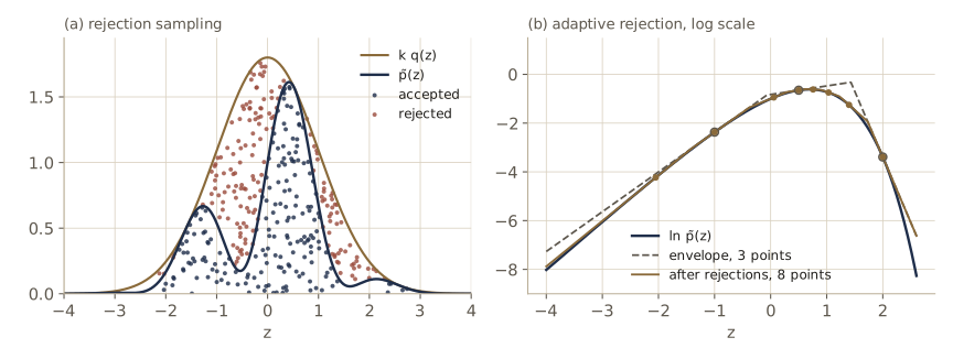
Suppose the target is \(p(z) = \widetilde{p}(z)/Z_p\), where we can evaluate the unnormalized density \(\widetilde{p}(z)\) but not the normalizing constant \(Z_p\). Rejection sampling uses a proposal distribution \(q(z)\) that we can sample from, and a constant \(k\) such that the comparison function \(k q(z)\) lies above \(\widetilde{p}(z)\) everywhere. Each step draws \(z_0 \sim q(z)\) and then \(u_0\) uniform on \([0, k q(z_0)]\). The pair \((z_0, u_0)\) is uniform under the curve \(k q(z)\). We keep \(z_0\) if \(u_0 \leq \widetilde{p}(z_0)\). The kept pairs are uniform under the curve \(\widetilde{p}(z)\), and the horizontal coordinate of a point uniform under a curve has that curve, normalized, as its density. So the kept \(z_0\) are exact samples from \(p(z)\).
A draw at \(z\) is accepted with probability \(\widetilde{p}(z)/k q(z)\), so the overall acceptance rate is
\[p(\text{accept}) = \int \frac{\widetilde{p}(z)}{k q(z)}\, q(z)\, \mathrm{d}z = \frac{Z_p}{k},\]the ratio of the area under \(\widetilde{p}\) to the area under \(k q\). The constant should be as small as the bound allows.
Our target is a wiggly bimodal density, \(\widetilde{p}(z) = e^{-z^2/2}\{1 + 0.8 \sin(3z)\}\). The sine term is odd, so it integrates to zero against the Gaussian and \(Z_p = \sqrt{2\pi}\); we will pretend not to know this when sampling and use it only to check. Using \(\mathbb{E}[z \sin(3z)] = 3 e^{-9/2}\) for a standard Gaussian, the exact mean is \(\mathbb{E}_p[z] = 2.4\, e^{-4.5} \approx 0.0267\). The proposal is \(\mathcal{N}(0, s^2)\); its tails must be at least as heavy as the target’s, so \(s \geq 1\). We find the smallest \(k\) by maximizing \(\widetilde{p}/q\) on a fine grid.
def p_tilde(z):
    """Unnormalized target: exp(-z^2/2) (1 + 0.8 sin 3z). Its normalizer is sqrt(2 pi)."""
    return np.exp(-0.5 * z ** 2) * (1 + 0.8 * np.sin(3 * z))

def gauss_pdf(z, s):
    return np.exp(-0.5 * (z / s) ** 2) / (np.sqrt(2 * np.pi) * s)

def envelope_constant(s):
    grid = np.linspace(-15, 15, 300_001)
    return 1.0001 * np.max(p_tilde(grid) / gauss_pdf(grid, s))   # small margin over the grid max

def rejection_sample(L, s, k, rng):
    """Propose L points from N(0, s^2); keep those with u0 <= p_tilde(z0), u0 ~ U[0, k q(z0)]."""
    z0 = s * rng.standard_normal(L)
    u0 = rng.random(L) * k * gauss_pdf(z0, s)
    keep = u0 <= p_tilde(z0)
    return z0[keep], keep.mean()

Zp, mean_exact = np.sqrt(2 * np.pi), 2.4 * np.exp(-4.5)
print("   s      k     Z_p/k   accepted   mean of samples +- standard error (exact 0.0267)")
for s in [1.0, 1.5, 2.0, 3.0]:
    k = envelope_constant(s)
    zs, acc = rejection_sample(200_000, s, k, rng)
    se = zs.std() / np.sqrt(len(zs))
    print(f"{s:4.1f}  {k:6.3f}   {Zp / k:.4f}   {acc:.4f}     {zs.mean():.4f} +- {se:.4f}")
   s      k     Z_p/k   accepted   mean of samples +- standard error (exact 0.0267)
 1.0   4.512   0.5555   0.5562     0.0204 +- 0.0030
 1.5   6.331   0.3959   0.3970     0.0229 +- 0.0036
 2.0   8.276   0.3029   0.3039     0.0317 +- 0.0041
 3.0  12.252   0.2046   0.2049     0.0203 +- 0.0050
The measured acceptance rates match \(Z_p/k\) to three decimals, and the sample means agree with the exact mean to within about two standard errors. The narrowest valid proposal wins: widening it wastes proposals in the tails, where the target has almost no mass.
That waste becomes catastrophic in high dimensions. Let the target be \(\mathcal{N}(\mathbf{0}, \mathbf{I})\) in \(D\) dimensions and the proposal \(\mathcal{N}(\mathbf{0}, \sigma_q^2 \mathbf{I})\) with \(\sigma_q\) just slightly larger than 1. The ratio \(p/q\) peaks at the origin, where it equals \(\sigma_q^D\), so \(k = \sigma_q^D\) and the acceptance rate is \(\sigma_q^{-D}\): exponentially small in \(D\) even though the two distributions look almost the same.
def gaussian_rejection_count(D, sigma_q, L, rng):
    """Number of accepted proposals out of L."""
    z = sigma_q * rng.standard_normal((L, D))
    # log of p(z) / (k q(z)) with k = sigma_q^D; both densities are normalized
    log_ratio = -0.5 * np.sum(z ** 2, axis=1) * (1 - 1 / sigma_q ** 2)
    return np.sum(np.log(rng.random(L)) < log_ratio)

L = 100_000
for D in [1, 10, 50, 100]:
    print(f"D = {D:3d}: accepted {gaussian_rejection_count(D, 1.1, L, rng):6d} of {L},"
          f"  expected L / 1.1^D = {L * 1.1 ** -D:9.1f}")
D =   1: accepted  90725 of 100000,  expected L / 1.1^D =   90909.1
D =  10: accepted  38807 of 100000,  expected L / 1.1^D =   38554.3
D =  50: accepted    830 of 100000,  expected L / 1.1^D =     851.9
D = 100: accepted      2 of 100000,  expected L / 1.1^D =       7.3
At \(D = 100\) we expect to accept 7 proposals in a hundred thousand and happened to get 2. An image has thousands of dimensions, and a realistic target is far less similar to any simple proposal than these two Gaussians are. Rejection sampling is a tool for one or two dimensions, or a subroutine inside a larger sampler.
Adaptive rejection sampling
Finding a tight envelope by hand is the hard part of rejection sampling. For a log-concave density, one whose logarithm \(h(z) = \ln \widetilde{p}(z)\) is concave, the envelope can be built automatically (Gilks and Wild, 1992). A concave function lies below each of its tangent lines, so the minimum of the tangents at a few points \(x_1 < \dots < x_m\),
\[u(z) = \min_j \left\{ h(x_j) + h'(x_j)(z - x_j) \right\},\]is a piecewise-linear upper bound on \(h\), and \(e^{u(z)}\) is a piecewise-exponential upper bound on \(\widetilde{p}\). Tangent \(j\) is the active piece between the points where it crosses its neighbors. The mass of each piece is an exponential integral in closed form, so sampling from the envelope takes two steps: pick a piece in proportion to its mass, then sample within the piece by the inverse-CDF method. A proposal \(z\) is accepted with probability \(e^{h(z) - u(z)}\). The adaptive part: when a proposal is rejected, we already paid for \(h(z)\), so we add \(z\) to the points. The envelope tightens exactly where it was loose, and the acceptance rate climbs toward 1.
Our log-concave target is \(h(z) = 2z - e^{z}\), the density of \(\ln g\) when \(g\) has a gamma distribution with shape 2. It is known to have mean \(\psi(2) \approx 0.4228\) and variance \(\psi'(2) = \pi^2/6 - 1 \approx 0.6449\), where \(\psi\) is the digamma function. For a piece with slope \(s \neq 0\) on \([a, b]\), write \(w = e^{-\lvert s\rvert (b - a)}\) and let \(t\) be the upper end \(b\) if \(s > 0\) and the lower end \(a\) if \(s < 0\); then the inverse CDF within the piece is \(z = t + s^{-1}\ln\{w + v(1 - w)\}\) with \(v\) uniform (exercise 3 asks you to derive it). This formula also covers the two unbounded end pieces, where \(w = 0\).
def ars(h, dh, x_init, L, rng):
    """Adaptive rejection sampling for a log-concave density exp(h). The first point must have
    h' > 0 and the last h' < 0, so that the two end pieces of the envelope are integrable."""
    xs = np.sort(np.asarray(x_init, dtype=float))
    samples, n_proposed = [], 0
    while len(samples) < L:
        s, c = dh(xs), h(xs) - dh(xs) * xs              # tangent j: c_j + s_j z
        cross = (c[1:] - c[:-1]) / (s[:-1] - s[1:])      # where tangent j meets tangent j+1
        a = np.concatenate([[-np.inf], cross])
        b = np.concatenate([cross, [np.inf]])
        w = np.exp(-np.abs(s) * (b - a))
        t = np.where(s > 0, b, a)
        log_mass = c + s * t + np.log1p(-w) - np.log(np.abs(s))
        j = rng.choice(len(xs), p=np.exp(log_mass - logsumexp(log_mass)))
        z = t[j] + np.log(w[j] + rng.random() * (1 - w[j])) / s[j]
        n_proposed += 1
        if np.log(rng.random()) < h(z) - (c[j] + s[j] * z):
            samples.append(z)
        else:
            xs = np.sort(np.append(xs, z))               # refine the envelope where it was loose
    return np.array(samples), len(xs), n_proposed

h = lambda z: 2 * z - np.exp(z)
dh = lambda z: 2 - np.exp(z)
for L in [100, 1000, 20_000]:
    zs, n_points, n_prop = ars(h, dh, [-1.0, 0.5, 2.0], L, np.random.default_rng(1))
    print(f"L = {L:6d}: {n_points:2d} hull points, acceptance {L / n_prop:.3f},"
          f"  mean {zs.mean():.4f}  var {zs.var():.4f}")
print(f"exact:  mean {digamma(2):.4f}  var {polygamma(1, 2):.4f}")
L =    100:  8 hull points, acceptance 0.952,  mean 0.4647  var 0.7123
L =   1000: 15 hull points, acceptance 0.988,  mean 0.4008  var 0.6442
L =  20000: 46 hull points, acceptance 0.998,  mean 0.4259  var 0.6453
exact:  mean 0.4228  var 0.6449
A handful of rejections is enough to make the envelope so tight that almost every later proposal is accepted, and the moments match the exact values. Log-concavity is common: the Gaussian, the logistic, the gamma with shape at least 1, and many posteriors of generalized linear models all have it. That makes adaptive rejection sampling a good inner step for Gibbs sampling, which we meet below. Versions exist that avoid derivatives and that handle densities that are not log-concave by adding a Metropolis–Hastings correction (Bishop & Bishop §14.1.4).
Importance sampling
Importance sampling estimates expectations without producing samples from \(p\) at all. Draw \(\mathbf{z}^{(l)}\) from a proposal \(q\) and reweight:
\[\mathbb{E}_p[f] = \int f(\mathbf{z}) \frac{p(\mathbf{z})}{q(\mathbf{z})}\, q(\mathbf{z})\, \mathrm{d}\mathbf{z} \approx \frac{1}{L} \sum_{l=1}^{L} r_l\, f(\mathbf{z}^{(l)}), \qquad r_l = \frac{p(\mathbf{z}^{(l)})}{q(\mathbf{z}^{(l)})}.\]The importance weights \(r_l\) correct for having sampled from the wrong distribution. The estimator is unbiased provided \(q > 0\) wherever \(p f \neq 0\). Unlike rejection sampling, nothing is thrown away, and no bound \(k\) is needed. The proposal should put its mass where \(p(\mathbf{z}) \lvert f(\mathbf{z}) \rvert\) is large, which may be far from where \(p\) itself is large. For the tail probability that defeated plain Monte Carlo, a proposal centred on the tail, \(q = \mathcal{N}(4, 1)\), gives weights \(r = e^{-4z + 8}\) and a precise answer from the same ten thousand draws:
L = 10_000
z = 4 + rng.standard_normal(L)                  # z ~ q = N(4, 1)
terms = (z > 4) * np.exp(-4 * z + 8)            # f(z) r(z) with r = N(z | 0, 1) / N(z | 4, 1)
print(f"importance sampling: {terms.mean():.4e} +- {terms.std() / np.sqrt(L):.1e}"
      f"   (exact {ndtr(-4):.4e})")
importance sampling: 3.1212e-05 +- 6.7e-07 (exact 3.1671e-05)
Self-normalized importance sampling. Usually both densities are known only up to constants, \(p = \widetilde{p}/Z_p\) and \(q = \widetilde{q}/Z_q\). With \(\widetilde{r}_l = \widetilde{p}(\mathbf{z}^{(l)})/\widetilde{q}(\mathbf{z}^{(l)})\), the average of the \(\widetilde{r}_l\) estimates \(Z_p/Z_q\), because \(\mathbb{E}_q[\widetilde{p}/\widetilde{q}] = \int \widetilde{p}\, \mathrm{d}\mathbf{z} / Z_q\). Dividing the unnormalized estimator by this average cancels the unknown constants and leaves a weighted average:
\[\mathbb{E}_p[f] \approx \sum_{l=1}^{L} w_l\, f(\mathbf{z}^{(l)}), \qquad w_l = \frac{\widetilde{r}_l}{\sum_{m} \widetilde{r}_m}.\]The weights are nonnegative and sum to one. The estimator is no longer exactly unbiased (it is a ratio of two estimates), but it is consistent, and it is the version used in practice. On the bimodal target of the last section, with the proposal \(\mathcal{N}(0, 1.5^2)\):
def self_normalized(log_p_tilde, log_q_tilde, z):
    """Normalized weights w_l, the estimate of Z_p / Z_q, and the effective sample size."""
    log_r = log_p_tilde(z) - log_q_tilde(z)
    w = np.exp(log_r - logsumexp(log_r))
    ratio = np.exp(logsumexp(log_r) - np.log(len(z)))
    return w, ratio, 1.0 / np.sum(w ** 2)

s_q = 1.5
z = s_q * rng.standard_normal(10_000)
w, ratio, ess = self_normalized(lambda z: np.log(p_tilde(z)),
                                lambda z: np.log(gauss_pdf(z, s_q)), z)   # this q is normalized
print(f"Z_p estimate {ratio:.4f} (exact {Zp:.4f})")
m = np.sum(w * z)
se = np.sqrt(np.sum(w ** 2 * (z - m) ** 2))        # standard error of a weighted average
print(f"E[z] estimate {m:.4f} +- {se:.4f} (exact {mean_exact:.4f})")
print(f"effective sample size {ess:.0f} of {len(z)}")
Z_p estimate 2.5265 (exact 2.5066)
E[z] estimate 0.0195 +- 0.0101 (exact 0.0267)
effective sample size 6314 of 10000
Both estimates are within their errors. The one for \(\mathbb{E}[z]\) is rough, because the weighted sample of 10,000 points is worth only about 6,300 unweighted ones, which brings us to the next idea.
Effective sample size. A weighted sample is worth less than an unweighted one of the same size, because a few heavy weights dominate the sum. A standard summary is the effective sample size
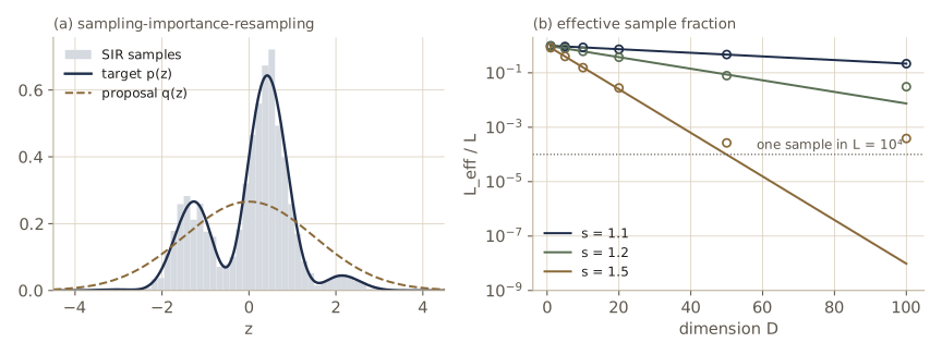
\[L_{\text{eff}} = \frac{\left( \sum_l \widetilde{r}_l \right)^2}{\sum_l \widetilde{r}_l^2} = \frac{1}{\sum_l w_l^2},\]which equals \(L\) when all weights are equal and 1 when a single weight carries everything. For large \(L\), \(L_{\text{eff}}/L \approx \mathbb{E}_q[r]^2 / \mathbb{E}_q[r^2]\). For a target \(\mathcal{N}(\mathbf{0}, \mathbf{I})\) and proposal \(\mathcal{N}(\mathbf{0}, s^2\mathbf{I})\) in \(D\) dimensions, a Gaussian integral (exercise 4) gives \(\mathbb{E}_q[r^2] = \{s^2/\sqrt{2s^2 - 1}\}^D\), so the effective fraction decays exponentially with dimension, just like the acceptance rate of rejection sampling:
def ess_fraction(D, s, L, rng):
    z = s * rng.standard_normal((L, D))
    log_r = -0.5 * np.sum(z ** 2, axis=1) * (1 - 1 / s ** 2)     # ln p - ln q up to a constant
    return np.exp(2 * logsumexp(log_r) - logsumexp(2 * log_r)) / L

print("  D   s = 1.1 (theory)        s = 1.5 (theory)")
for D in [1, 10, 50, 100]:
    row = [(ess_fraction(D, s, 10_000, rng), (np.sqrt(2 * s**2 - 1) / s**2) ** D)
           for s in (1.1, 1.5)]
    print(f"{D:3d}   " + "    ".join(f"{m:.2e} ({t:.2e})" for m, t in row))
  D   s = 1.1 (theory)        s = 1.5 (theory)
  1   9.85e-01 (9.85e-01)    8.34e-01 (8.31e-01)
 10   8.58e-01 (8.58e-01)    1.56e-01 (1.58e-01)
 50   4.67e-01 (4.66e-01)    1.33e-03 (9.83e-05)
100   2.23e-01 (2.17e-01)    1.29e-04 (9.66e-09)
For \(s = 1.1\) the measurements follow the theory, and even at \(D = 100\) a fifth of the samples still count. For \(s = 1.5\) the fraction falls to about \(10^{-4}\) at \(D = 50\) and \(10^{-8}\) at \(D = 100\), and there the measured values are too optimistic, by factors of ten and ten thousand. The expectation \(\mathbb{E}_q[r^2]\) is dominated by enormous weights that occur so rarely that 10,000 draws do not contain them, so the measured effective sample size looks acceptable while the estimate itself rests on a few points. The same collapse happens in one dimension when \(q\) is displaced from \(p\). A dangerous feature is that it can go unnoticed: if no sample lands where \(p f\) is large, the weights can look well behaved and the estimate can be badly wrong with nothing to warn us. The requirement to remember is that \(q\) must not be small where \(p\) is appreciable; a proposal with heavier tails than the target is the safe choice.
In practice. Importance sampling is at its best when a good proposal is available, and in deep learning one often is. In module 16 a Gaussian placed near the posterior of a latent-variable model estimates \(\ln p(\mathbf{x})\) with a handful of samples where sampling from the prior needs thousands; a trained encoder (module 19) provides such a proposal for every input. Always report the effective sample size alongside the estimate.
Sampling-importance-resampling
Importance weights give expectations, but sometimes we want actual samples, and rejection sampling would need a bound \(k\) that may not exist or may be uselessly large. Sampling-importance-resampling (SIR) needs no bound. Draw \(\mathbf{z}^{(1)}, \dots, \mathbf{z}^{(L)}\) from \(q\), compute the normalized weights \(w_l\), and then draw a new set of \(L\) values from the discrete distribution that puts probability \(w_l\) on \(\mathbf{z}^{(l)}\).
The resampled values are only approximately distributed as \(p\), but the approximation becomes exact as \(L \to \infty\). In one dimension, the probability that a resampled value is at most \(a\) is \(\sum_l w_l\, I(z^{(l)} \leq a)\), a ratio of two importance-sampling averages. As \(L\) grows each average converges to its integral, \(\int I(z \leq a)\, \widetilde{p}(z)\, \mathrm{d}z / Z_q\) over \(\int \widetilde{p}(z)\, \mathrm{d}z / Z_q\), and the ratio is the CDF of \(p\). We measure the gap with the largest difference between the empirical CDF of the resampled values and the exact CDF (the Kolmogorov–Smirnov distance), which we compute for our target on a fine grid.
grid = np.linspace(-8, 8, 160_001)
cdf_exact = np.cumsum(p_tilde(grid)) * (grid[1] - grid[0]) / Zp

def ks_distance(samples):
    x = np.sort(samples)
    F = np.interp(x, grid, cdf_exact)
    n = len(x)
    return max(np.max(np.arange(1, n + 1) / n - F), np.max(F - np.arange(n) / n))

def sir(L, s_q, rng):
    z = s_q * rng.standard_normal(L)
    w, _, _ = self_normalized(lambda z: np.log(p_tilde(z)), lambda z: np.log(gauss_pdf(z, s_q)), z)
    return z[rng.choice(L, size=L, p=w)]

for L in [100, 1000, 10_000, 100_000]:
    d_sir = np.mean([ks_distance(sir(L, 1.5, rng)) for _ in range(20)])
    print(f"L = {L:6d}: KS distance of SIR samples {d_sir:.4f}   (typical for exact samples"
          f" {0.87 / np.sqrt(L):.4f})")
L =    100: KS distance of SIR samples 0.1226   (typical for exact samples 0.0870)
L =   1000: KS distance of SIR samples 0.0422   (typical for exact samples 0.0275)
L =  10000: KS distance of SIR samples 0.0125   (typical for exact samples 0.0087)
L = 100000: KS distance of SIR samples 0.0047   (typical for exact samples 0.0028)
The distance shrinks like \(1/\sqrt{L}\), a little above what exact independent samples would give, because resampling duplicates heavily weighted points. If moments are all we need, it is better to skip the resampling step and use the weighted original sample, which carries slightly less noise. SIR resurfaces in sequential Monte Carlo (particle filters), where a population of weighted samples is resampled at every time step.
Markov chain Monte Carlo
Rejection and importance sampling draw each proposal from a fixed distribution, blind to where the earlier proposals landed. In high dimensions a fixed distribution almost never matches the target well, and both methods collapse. Markov chain Monte Carlo proposes locally instead: it keeps a current state \(\mathbf{z}^{(\tau)}\), proposes a candidate \(\mathbf{z}^{\star}\) from a distribution \(q(\mathbf{z} \mid \mathbf{z}^{(\tau)})\) that depends on it, and accepts or rejects the candidate by a rule designed so that, in the long run, the states are distributed according to \(p(\mathbf{z}) = \widetilde{p}(\mathbf{z})/Z_p\). As before, only \(\widetilde{p}\) has to be evaluated. The price is that consecutive states are correlated.
The Metropolis algorithm
The Metropolis algorithm (Metropolis et al., 1953) uses a symmetric proposal, \(q(\mathbf{z}_A \mid \mathbf{z}_B) = q(\mathbf{z}_B \mid \mathbf{z}_A)\), such as a Gaussian step \(\mathbf{z}^{\star} = \mathbf{z}^{(\tau)} + \rho\, \boldsymbol{\epsilon}\) with \(\boldsymbol{\epsilon} \sim \mathcal{N}(\mathbf{0}, \mathbf{I})\). The candidate is accepted with probability
\[A(\mathbf{z}^{\star}, \mathbf{z}^{(\tau)}) = \min\left( 1, \frac{\widetilde{p}(\mathbf{z}^{\star})}{\widetilde{p}(\mathbf{z}^{(\tau)})} \right).\]Uphill moves are always accepted; downhill moves are accepted with a probability equal to the density ratio. If the candidate is accepted, \(\mathbf{z}^{(\tau+1)} = \mathbf{z}^{\star}\); if not, the chain stays where it is and \(\mathbf{z}^{(\tau+1)} = \mathbf{z}^{(\tau)}\), and the repeated state counts again as a sample. Dropping the repeats (as rejection sampling drops rejected points) would bias the result. We work with \(\ln \widetilde{p}\) to avoid underflow.
def metropolis(log_p, z0, rho, T, rng):
    """Random-walk Metropolis with proposal z* = z + rho eps. Returns the T states and the
    acceptance rate. A rejected candidate repeats the current state."""
    z = np.array(z0, dtype=float)
    lp = log_p(z)
    chain, n_acc = np.empty((T, z.size)), 0
    eps, log_u = rng.standard_normal((T, z.size)), np.log(rng.random(T))
    for t in range(T):
        z_star = z + rho * eps[t]
        lp_star = log_p(z_star)
        if log_u[t] < lp_star - lp:                  # u < p(z*) / p(z)
            z, lp = z_star, lp_star
            n_acc += 1
        chain[t] = z
    return chain, n_acc / T
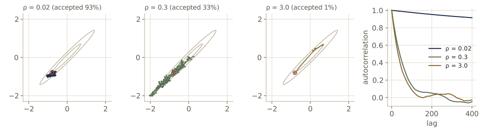
Our test target is a strongly correlated two-dimensional Gaussian: standard deviation \(\sigma_{\max} = 1\) along the diagonal and \(\sigma_{\min} = 0.1\) across it, a stand-in for the long, narrow ridges that posteriors over network weights tend to have.
R = np.array([[1, -1], [1, 1]]) / np.sqrt(2)          # columns: long axis, short axis
sig_max, sig_min = 1.0, 0.1
Lambda = R @ np.diag([1 / sig_max ** 2, 1 / sig_min ** 2]) @ R.T   # precision matrix

def log_p_ridge(z):
    return -0.5 * z @ Lambda @ z

chain, acc = metropolis(log_p_ridge, [0.0, 0.0], 0.1, 50_000, rng)
print(f"acceptance {acc:.3f}")
print("sample covariance\n", np.cov(chain[5000:].T))
print("exact covariance\n", np.linalg.inv(Lambda))
acceptance 0.702
sample covariance
 [[0.5308 0.52  ]
 [0.52   0.5298]]
exact covariance
 [[0.505 0.495]
 [0.495 0.505]]
The covariance is close, but not very close, after fifty thousand steps; the error of about 0.03 in each entry is what we will see is typical for a chain this correlated. The reason is that a chain of small symmetric steps behaves like a random walk. For a walk that steps \(\pm 1\) with equal probability, \(\mathbb{E}[(z^{(\tau)})^2] = \mathbb{E}[(z^{(\tau-1)})^2] + 1\), since the step is independent of the position and has zero mean. So after \(\tau\) steps the typical distance travelled is only \(\sqrt{\tau}\):
walks = np.cumsum(rng.choice([-1, 1], size=(5000, 400)), axis=1)
for tau in [25, 100, 400]:
    print(f"tau = {tau:3d}: E[z^2] = {np.mean(walks[:, tau - 1] ** 2):6.1f},"
          f"  RMS distance {np.sqrt(np.mean(walks[:, tau - 1] ** 2)):5.1f}")
tau =  25: E[z^2] =   23.8,  RMS distance   4.9
tau = 100: E[z^2] =   95.1,  RMS distance   9.8
tau = 400: E[z^2] =  382.7,  RMS distance  19.6
To cover a distance \(d\) with steps of size \(\rho\) takes about \((d/\rho)^2\) steps, not \(d/\rho\). Much of the design of better MCMC methods, including the gradient-based Langevin methods at the end of this module, is about suppressing this random-walk behavior.
Markov chains
To see why Metropolis works, and when MCMC can fail, we need a few facts about Markov chains. A first-order Markov chain is a sequence \(\mathbf{z}^{(1)}, \mathbf{z}^{(2)}, \dots\) in which each state depends on the past only through its predecessor, \(p(\mathbf{z}^{(m+1)} \mid \mathbf{z}^{(1)}, \dots, \mathbf{z}^{(m)}) = p(\mathbf{z}^{(m+1)} \mid \mathbf{z}^{(m)})\), the chain-shaped graph of module 11. It is specified by the initial distribution and the transition probabilities \(T(\mathbf{z}', \mathbf{z}) = p(\mathbf{z}^{(m+1)} = \mathbf{z} \mid \mathbf{z}^{(m)} = \mathbf{z}')\), and it is homogeneous if these are the same at every step. The marginals then evolve as
\[p(\mathbf{z}^{(m+1)}) = \int T(\mathbf{z}', \mathbf{z}^{(m+1)})\, p(\mathbf{z}^{(m)} = \mathbf{z}')\, \mathrm{d}\mathbf{z}'.\]Definition. A distribution \(p^{\star}\) is invariant (or stationary) for the chain if one step leaves it unchanged, \(p^{\star}(\mathbf{z}) = \int T(\mathbf{z}', \mathbf{z})\, p^{\star}(\mathbf{z}')\, \mathrm{d}\mathbf{z}'\). The chain satisfies detailed balance with respect to \(p^{\star}\) if \(p^{\star}(\mathbf{z})\, T(\mathbf{z}, \mathbf{z}') = p^{\star}(\mathbf{z}')\, T(\mathbf{z}', \mathbf{z})\) for all pairs; such a chain is called reversible. The chain is ergodic if \(p(\mathbf{z}^{(m)})\) converges to \(p^{\star}\) from every starting distribution; \(p^{\star}\) is then the unique equilibrium distribution.
Detailed balance says that, in equilibrium, the flow of probability from \(\mathbf{z}\) to \(\mathbf{z}'\) equals the flow back. It implies invariance: integrating both sides over \(\mathbf{z}'\),
\[\int p^{\star}(\mathbf{z}')\, T(\mathbf{z}', \mathbf{z})\, \mathrm{d}\mathbf{z}' = p^{\star}(\mathbf{z}) \int T(\mathbf{z}, \mathbf{z}')\, \mathrm{d}\mathbf{z}' = p^{\star}(\mathbf{z}),\]since the transition probabilities out of \(\mathbf{z}\) sum to one. The converse fails: a chain can leave \(p^{\star}\) invariant without being reversible. Invariance alone is not enough either. The identity transition leaves every distribution invariant and converges to nothing. Ergodicity holds under mild conditions, for instance when every state can reach every other and the chain is not periodic (Neal, 1993, gives the details).
On a finite state space all of this is linear algebra. With \(T_{ij}\) the probability of moving from state \(i\) to state \(j\), a row vector of marginals evolves as \(\boldsymbol{\pi}^{(m+1)} = \boldsymbol{\pi}^{(m)}\mathbf{T}\), so an invariant distribution is a left eigenvector of \(\mathbf{T}\) with eigenvalue 1, and the other eigenvalues set how fast the chain forgets its start. We build the Metropolis chain for a target on five states, proposing a move one step left or right with probability \(\tfrac12\) each (a move off the end is rejected), and check everything:
def metropolis_matrix(pi, proposal):
    """Transition matrix: propose j from row i of `proposal`, accept with min(1, pi_j / pi_i)."""
    K = len(pi)
    T = proposal * np.minimum(1, pi[None, :] / pi[:, None])
    T[np.arange(K), np.arange(K)] = 0
    T[np.arange(K), np.arange(K)] = 1 - T.sum(axis=1)       # rejected mass stays put
    return T

pi_tilde = np.array([1.0, 3.0, 6.0, 3.0, 2.0])               # unnormalized target
pi = pi_tilde / pi_tilde.sum()
Q_nbr = 0.5 * (np.eye(5, k=1) + np.eye(5, k=-1))             # propose a neighbor
B1 = metropolis_matrix(pi, Q_nbr)

flow = pi[:, None] * B1                                       # flow_ij = pi_i T_ij
print("rows sum to one:", np.allclose(B1.sum(axis=1), 1))
print("detailed balance, max |pi_i T_ij - pi_j T_ji|:", f"{np.abs(flow - flow.T).max():.1e}")
lam, V = np.linalg.eig(B1.T)                                  # left eigenvectors of T
order = np.argsort(-np.abs(lam))
v = np.real(V[:, order[0]])
print("eigenvalues:", np.real(lam[order]))
print("eigenvector for eigenvalue 1, normalized:", v / v.sum())
print("target pi:                               ", pi)
rows sum to one: True
detailed balance, max |pi_i T_ij - pi_j T_ji|: 0.0e+00
eigenvalues: [ 1.      0.7477  0.5    -0.2807  0.0331]
eigenvector for eigenvalue 1, normalized: [0.0667 0.2    0.4    0.2    0.1333]
target pi:                                [0.0667 0.2    0.4    0.2    0.1333]
The eigenvector for eigenvalue 1 is the target, and the second-largest eigenvalue in magnitude, \(\lvert\lambda_2\rvert\), controls convergence: the distance to equilibrium shrinks roughly like \(\lvert\lambda_2\rvert^m\). Starting from state 0 with certainty:
p_m = np.eye(5)[0]
lam2 = np.abs(lam[order[1]])
for m in range(1, 41):
    p_m = p_m @ B1
    if m in (1, 5, 10, 20, 40):
        tv = 0.5 * np.abs(p_m - pi).sum()
        print(f"m = {m:2d}: total variation to pi {tv:.2e}   |lambda_2|^m {lam2 ** m:.2e}")
m =  1: total variation to pi 7.33e-01   |lambda_2|^m 7.48e-01
m =  5: total variation to pi 1.70e-01   |lambda_2|^m 2.34e-01
m = 10: total variation to pi 4.27e-02   |lambda_2|^m 5.46e-02
m = 20: total variation to pi 2.35e-03   |lambda_2|^m 2.98e-03
m = 40: total variation to pi 7.01e-06   |lambda_2|^m 8.87e-06
In practice a transition is often assembled from simpler base transitions \(B_1, \dots, B_K\), each of which leaves \(p^{\star}\) invariant, either as a mixture \(\sum_k \alpha_k B_k\) or by applying them in sequence, \(B_1 B_2 \cdots B_K\) (each changing only some of the variables, for instance). Both combinations keep \(p^{\star}\) invariant. A mixture of reversible transitions is reversible, but a sequence generally is not; applying the sequence forward and then backward, \(B_1 \cdots B_K B_K \cdots B_1\), restores detailed balance. We add a second base transition that proposes any state uniformly and test the three combinations:
B2 = metropolis_matrix(pi, np.full((5, 5), 0.2))          # propose any state uniformly

def check(name, T):
    flow = pi[:, None] * T
    print(f"{name:14s} invariant: {np.allclose(pi @ T, pi)}   "
          f"detailed balance: {np.allclose(flow, flow.T)}")

check("0.5 B1 + 0.5 B2", 0.5 * B1 + 0.5 * B2)
check("B1 B2", B1 @ B2)
check("B1 B2 B2 B1", B1 @ B2 @ B2 @ B1)
0.5 B1 + 0.5 B2 invariant: True   detailed balance: True
B1 B2          invariant: True   detailed balance: False
B1 B2 B2 B1    invariant: True   detailed balance: True
The Metropolis–Hastings algorithm
The Metropolis–Hastings algorithm (Hastings, 1970) allows proposals that are not symmetric. With the proposal \(q_k(\mathbf{z} \mid \mathbf{z}^{(\tau)})\) (the label \(k\) indexes a set of possible transitions, as in the base transitions above), the acceptance probability becomes
\[A_k(\mathbf{z}^{\star}, \mathbf{z}^{(\tau)}) = \min\left( 1, \frac{\widetilde{p}(\mathbf{z}^{\star})\, q_k(\mathbf{z}^{(\tau)} \mid \mathbf{z}^{\star})}{\widetilde{p}(\mathbf{z}^{(\tau)})\, q_k(\mathbf{z}^{\star} \mid \mathbf{z}^{(\tau)})} \right).\]The extra factor corrects for a proposal that moves more easily in one direction than the other; for a symmetric proposal it cancels and we recover Metropolis. The normalizer \(Z_p\) cancels as before.
Why it works. We show detailed balance for \(\mathbf{z} \neq \mathbf{z}'\) (the case \(\mathbf{z} = \mathbf{z}'\) is trivial). The transition density is the proposal times the acceptance probability, so
\[\begin{aligned} p(\mathbf{z})\, q_k(\mathbf{z}' \mid \mathbf{z})\, A_k(\mathbf{z}', \mathbf{z}) &= \min\left( p(\mathbf{z})\, q_k(\mathbf{z}' \mid \mathbf{z}),\; p(\mathbf{z}')\, q_k(\mathbf{z} \mid \mathbf{z}') \right) \\ &= p(\mathbf{z}')\, q_k(\mathbf{z} \mid \mathbf{z}')\, A_k(\mathbf{z}, \mathbf{z}'). \end{aligned}\]The first line multiplies \(p(\mathbf{z})q_k(\mathbf{z}' \mid \mathbf{z})\) into the minimum; the expression is symmetric in \(\mathbf{z}\) and \(\mathbf{z}'\), and the second line pulls the other product back out. So \(p\) is invariant, and with a proposal that can reach every state the chain is ergodic.
The correction factor matters. A natural proposal for a positive variable is a multiplicative step \(z^{\star} = z\, e^{\sigma\epsilon}\), whose density is log-normal and asymmetric: \(q(z \mid z^{\star})/q(z^{\star} \mid z) = z^{\star}/z\). We sample a gamma density \(\widetilde{p}(z) = z^2 e^{-z}\) (mean 3) with and without the correction.
def mh_positive(log_p, z0, sigma, T, rng, hastings=True):
    """Metropolis-Hastings with the multiplicative proposal z* = z exp(sigma eps)."""
    z, lp, out = z0, log_p(z0), np.empty(T)
    for t, (e, lu) in enumerate(zip(rng.standard_normal(T), np.log(rng.random(T)))):
        z_star = z * np.exp(sigma * e)
        lp_star = log_p(z_star)
        log_A = lp_star - lp + (np.log(z_star) - np.log(z) if hastings else 0.0)
        if lu < log_A:
            z, lp = z_star, lp_star
        out[t] = z
    return out

log_gamma3 = lambda z: 2 * np.log(z) - z
for hastings in (True, False):
    zs = mh_positive(log_gamma3, 1.0, 0.8, 100_000, rng, hastings)[5000:]
    print(f"Hastings correction {str(hastings):5s}: mean {zs.mean():.3f}  var {zs.var():.3f}")
print("target Gamma(3, 1): mean 3, var 3")
Hastings correction True : mean 2.989  var 2.973
Hastings correction False: mean 2.001  var 2.049
target Gamma(3, 1): mean 3, var 3
With the correction the moments match. Without it the chain is an ordinary Metropolis chain for \(\ln z\) that forgets the Jacobian of the change of variables, and it samples a density proportional to \(\widetilde{p}(z)/z = z e^{-z}\), a gamma density with mean 2 and variance 2, which is what we see.
Choosing the proposal scale. For a Gaussian random-walk proposal of scale \(\rho\) there is a trade-off. A small \(\rho\) gets almost every step accepted but moves slowly, and a large \(\rho\) proposes big moves that are almost all rejected. Both produce highly correlated chains. We quantify the correlation with the autocorrelation \(\rho_k\) of a scalar summary of the chain at lag \(k\), and with the integrated autocorrelation time
\[\tau_{\text{int}} = 1 + 2\sum_{k=1}^{\infty} \rho_k .\]The variance of a chain average over \(T\) steps is approximately \(\tau_{\text{int}}\) times that of \(T\) independent samples, so the chain is worth \(T/\tau_{\text{int}}\) independent samples, its effective sample size. We estimate the sum with a standard self-consistent window (stop at the first lag \(M \geq 5\,\tau(M)\)) and track the coordinate along the long axis of the ridge, the slowest direction.
def autocorr(x, max_lag):
    """Autocorrelation of a 1-D series for lags 0..max_lag, via the FFT."""
    x = x - x.mean()
    f = np.fft.rfft(x, 2 * len(x))
    acf = np.fft.irfft(f * np.conj(f))[:max_lag + 1]
    return acf / acf[0]

def integrated_time(x):
    if np.var(x) == 0:
        return np.nan                             # the chain never moved
    acf = autocorr(x, len(x) // 4)
    tau = 2 * np.cumsum(acf) - 1                  # tau(M) = 1 + 2 sum_{k=1}^{M} rho_k
    M = np.arange(len(tau))
    ok = M >= 5 * tau
    return tau[np.argmax(ok)] if ok.any() else np.nan   # nan: chain too short to tell

def axis_ridge(D):
    """ln p for a Gaussian with std sig_max along z_1 and sig_min along the other D - 1 axes."""
    prec = np.full(D, 1 / sig_min ** 2)
    prec[0] = 1 / sig_max ** 2
    return lambda z: -0.5 * np.sum(prec * z ** 2)

T = 50_000
print("          D = 2 (one narrow axis)       D = 10 (nine narrow axes)")
print("   rho   acceptance  tau_int   ESS     acceptance  tau_int   ESS")
for rho in [0.02, 0.05, 0.1, 0.3, 1.0, 3.0]:
    row = ""
    for D in (2, 10):
        chain, acc = metropolis(axis_ridge(D), np.zeros(D), rho, T, rng)
        tau = integrated_time(chain[:, 0])        # the slow coordinate, along the long axis
        row += (f"     {acc:.3f}  {tau:8.1f}  {T / tau:5.0f}" if np.isfinite(tau)
                else f"     {acc:.3f}     >{T // 20}      <20")
    print(f"{rho:6.2f}" + row)
          D = 2 (one narrow axis)       D = 10 (nine narrow axes)
   rho   acceptance  tau_int   ESS     acceptance  tau_int   ESS
  0.02     0.936     >2500      <20     0.771     >2500      <20
  0.05     0.845    1071.8     47     0.474     >2500      <20
  0.10     0.701     365.9    137     0.172    1048.6     48
  0.30     0.365     128.2    390     0.001     >2500      <20
  1.00     0.102      60.8    823     0.000     >2500      <20
  3.00     0.019     117.9    424     0.000     >2500      <20
Rotating the ridge to the axes changes nothing for an isotropic proposal, so we use axis-aligned targets. In both columns the smallest scales accept almost everything and hardly move, and the chains are worth fewer than 20 independent samples. Large scales fail in the opposite way. With nine narrow directions, a proposal of 0.3 lands outside the narrow band in almost every direction at once and is almost never accepted, so the best scale is about \(\sigma_{\min}\), and even there \(\tau_{\text{int}}\) is about a thousand. The chain explores the long axis by a random walk with steps of order \(\sigma_{\min}\), so the number of steps between nearly independent states grows like \((\sigma_{\max}/\sigma_{\min})^2 = 100\), times a constant. In two dimensions the picture is more forgiving: large proposals are rejected more often, but each accepted one jumps far, and the two effects roughly cancel over a wide range of \(\rho\). The general statement (Neal, 1993; Bishop & Bishop §14.2.3) is that the cost is set by the ratio of the largest to the second-smallest width, which in two dimensions is 1. Real targets, such as posteriors over many weights, have many narrow directions, and the ten-dimensional column is the realistic one. That is why reparameterizing a model so that its posterior is closer to isotropic helps so much.
Gibbs sampling
Gibbs sampling (Geman and Geman, 1984) updates one variable at a time by drawing it from its conditional distribution given all the others. For \(\mathbf{z} = (z_1, \dots, z_M)\), one sweep replaces \(z_1\) by a draw from \(p(z_1 \mid z_2, \dots, z_M)\), then \(z_2\) by a draw from \(p(z_2 \mid z_1, z_3, \dots, z_M)\) using the new \(z_1\), and so on through \(z_M\). The variables can also be visited in random order.
Each update leaves \(p\) invariant: it does not touch \(\mathbf{z}_{\setminus i}\) (all variables except \(z_i\)), so their marginal is unchanged, and it draws \(z_i\) from the correct conditional given them, so the joint \(p(z_i \mid \mathbf{z}_{\setminus i})\, p(\mathbf{z}_{\setminus i})\) is reproduced. A sweep is a sequence of such base transitions and is therefore invariant too. Ergodicity needs a separate argument; it holds, for example, when no conditional is zero anywhere, because then any state can be reached from any other in one sweep.
Gibbs sampling is Metropolis–Hastings with an acceptance rate of exactly one. Take the proposal for variable \(k\) to be \(q_k(\mathbf{z}^{\star} \mid \mathbf{z}) = p(z_k^{\star} \mid \mathbf{z}_{\setminus k})\) with \(\mathbf{z}^{\star}_{\setminus k} = \mathbf{z}_{\setminus k}\). Writing \(p(\mathbf{z}) = p(z_k \mid \mathbf{z}_{\setminus k})\, p(\mathbf{z}_{\setminus k})\),
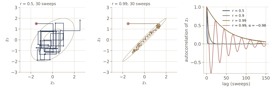
\[\frac{p(\mathbf{z}^{\star})\, q_k(\mathbf{z} \mid \mathbf{z}^{\star})}{p(\mathbf{z})\, q_k(\mathbf{z}^{\star} \mid \mathbf{z})} = \frac{p(z_k^{\star} \mid \mathbf{z}_{\setminus k})\, p(\mathbf{z}_{\setminus k})\, p(z_k \mid \mathbf{z}_{\setminus k})}{p(z_k \mid \mathbf{z}_{\setminus k})\, p(\mathbf{z}_{\setminus k})\, p(z_k^{\star} \mid \mathbf{z}_{\setminus k})} = 1 .\]So no step is wasted on rejections. The catch is the same random walk as before, now along the coordinate axes. Take a bivariate Gaussian with unit variances and correlation \(r\). Its conditionals are \(z_1 \mid z_2 \sim \mathcal{N}(r z_2, 1 - r^2)\) and symmetrically for \(z_2\). Each update moves by about the conditional width \(\sqrt{1 - r^2}\), while the distribution extends about \(\sqrt{1 + r}\) along the diagonal. Substituting one update into the next shows that the sequence of \(z_1\) values after each sweep is an autoregressive process \(z_1' = r^2 z_1 + \text{noise}\), so its autocorrelation at lag \(k\) is \(r^{2k}\) and \(\tau_{\text{int}} = (1 + r^2)/(1 - r^2)\).
Over-relaxation (Adler, 1981) is a cheap improvement when the conditionals are Gaussian. Instead of a fresh draw, replace \(z_i\) by
\[z_i' = \mu_i + \alpha(z_i - \mu_i) + \sigma_i \sqrt{1 - \alpha^2}\, \nu, \qquad \nu \sim \mathcal{N}(0, 1),\]where \(\mu_i\) and \(\sigma_i^2\) are the conditional mean and variance and \(-1 < \alpha < 1\). If \(z_i\) has the conditional distribution, so does \(z_i'\) (mean \(\mu_i\), variance \(\alpha^2\sigma_i^2 + (1 - \alpha^2)\sigma_i^2 = \sigma_i^2\)), so the update is still valid. With \(\alpha = 0\) it is ordinary Gibbs; with \(\alpha\) close to \(-1\) it reflects \(z_i\) to the other side of the conditional mean, which tends to keep the chain moving in the same direction along the ridge instead of diffusing.
def gibbs_bivariate(r, T, rng, alpha=0.0, z0=(0.0, 0.0)):
    """Systematic-scan Gibbs (alpha = 0) or over-relaxed Gibbs for a bivariate Gaussian
    with unit variances and correlation r. Returns the state after each sweep."""
    z1, z2 = z0
    s = np.sqrt(1 - r ** 2)                        # conditional standard deviation
    c = s * np.sqrt(1 - alpha ** 2)
    nu = rng.standard_normal((T, 2))
    chain = np.empty((T, 2))
    for t in range(T):
        mu = r * z2
        z1 = mu + alpha * (z1 - mu) + c * nu[t, 0]     # z1 | z2 ~ N(r z2, 1 - r^2)
        mu = r * z1
        z2 = mu + alpha * (z2 - mu) + c * nu[t, 1]
        chain[t] = z1, z2
    return chain

T = 100_000
print("   r    alpha   lag-1 corr (r^2)   tau_int (theory)   corr(z1, z2)")
for r, alpha in [(0.5, 0.0), (0.9, 0.0), (0.99, 0.0), (0.99, -0.9), (0.99, -0.98)]:
    ch = gibbs_bivariate(r, T, rng, alpha)
    tau = integrated_time(ch[:, 0])
    theory = f"({(1 + r**2) / (1 - r**2):6.1f})" if alpha == 0 else "        "
    print(f"{r:5.2f}  {alpha:6.2f}   {autocorr(ch[:, 0], 1)[1]:.4f} ({r**2:.4f})"
          f"    {tau:8.1f} {theory}     {np.corrcoef(ch.T)[0, 1]:.3f}")
   r    alpha   lag-1 corr (r^2)   tau_int (theory)   corr(z1, z2)
 0.50    0.00   0.2530 (0.2500)         1.7 (   1.7)     0.499
 0.90    0.00   0.8107 (0.8100)         9.5 (   9.5)     0.901
 0.99    0.00   0.9788 (0.9801)        86.4 (  99.5)     0.989
 0.99   -0.90   0.9624 (0.9801)         5.8              0.990
 0.99   -0.98   0.9607 (0.9801)         1.2              0.990
The lag-1 correlations match \(r^2\), and the autocorrelation times match the formula to within the estimation error of \(\tau_{\text{int}}\) itself, which is about 15% for the slowest chain. For weak correlation Gibbs sampling is nearly as good as independent sampling; at \(r = 0.99\) it needs about a hundred sweeps per independent sample. Over-relaxation with \(\alpha\) near \(-1\) cuts that dramatically without changing the distribution sampled (the correlation stays at 0.99). Its lag-1 correlation is still high, but its autocorrelation then oscillates and turns negative, because the chain keeps overshooting the conditional mean in alternating directions, and positive and negative terms cancel in \(\tau_{\text{int}}\). In this Gaussian example we could also have rotated to uncorrelated coordinates, but for real models such a rotation is rarely available.
Gibbs sampling is attractive whenever the conditionals are easy to sample. In a directed graphical model the conditional of a node given all the others depends only on its Markov blanket (its parents, children, and co-parents; see module 11), so each update is a local computation. When a conditional is not a standard distribution but is log-concave, which is common for directed models, adaptive rejection sampling handles it. To weaken the dependence between successive states one can also update groups of variables jointly, blocking Gibbs sampling, at the cost of harder conditionals. The restricted Boltzmann machine, an early deep-learning model, is designed so that all hidden units are conditionally independent given the visible ones and vice versa, so a whole layer is one block.
Ancestral sampling
For a directed graphical model with no observed variables, no Markov chain is needed. The joint distribution factorizes as \(p(\mathbf{z}) = \prod_i p(z_i \mid \mathrm{pa}(i))\), so ancestral sampling draws the nodes in a topological order, each from its conditional given its already-drawn parents, and one pass produces an exact sample from the joint. Module 11 implements it, and every latent-variable model in the second half of the course (sample \(\mathbf{z}\), then run the decoder) is sampled this way.
Things change when some nodes are observed, the evidence set, and we want the posterior over the rest. Logic sampling runs ancestral sampling and throws away every sample that disagrees with the evidence. It is exact but, like rejection sampling, its acceptance rate is the probability of the evidence, which shrinks rapidly as more variables are observed. Likelihood weighting clamps each observed node to its value instead of sampling it, and gives the sample the importance weight \(r = \prod_{i \in \text{evidence}} p(z_i \mid \mathrm{pa}(i))\): the proposal is the product of the conditionals of the unobserved nodes, so the ratio of target to proposal is just the product of the clamped factors. We try both on a small model of a web service: a server overload \(S\) and a slow network \(N\) each raise the chance of a page timeout \(T\), and a timeout usually triggers an alert \(A\). Given \(T = 1\) and \(A = 1\), how likely is an overload?
p_S, p_N = 0.1, 0.2
p_T = np.array([[0.02, 0.3], [0.6, 0.9]])      # p(T = 1 | S, N), indexed [S, N]
p_A = np.array([0.05, 0.8])                     # p(A = 1 | T)

# exact posterior by enumeration: p(S, N | T=1, A=1) is proportional to
# p(S) p(N) p(T=1 | S, N) p(A=1 | T=1)
joint = np.array([[(p_S if s else 1 - p_S) * (p_N if n else 1 - p_N) * p_T[s, n] * p_A[1]
                   for n in (0, 1)] for s in (0, 1)])
print(f"exact p(S = 1 | T = 1, A = 1) = {joint[1].sum() / joint.sum():.4f}")

L = 20_000
S = rng.random(L) < p_S                         # ancestral sampling, parents first
N = rng.random(L) < p_N
Tn = rng.random(L) < p_T[S.astype(int), N.astype(int)]
A = rng.random(L) < p_A[Tn.astype(int)]
keep = Tn & A                                   # logic sampling: discard disagreements
se = S[keep].std() / np.sqrt(keep.sum())
print(f"logic sampling:       {S[keep].mean():.4f} +- {se:.4f}"
      f"  (kept {keep.mean():.3f} of the samples)")

r = p_T[S.astype(int), N.astype(int)] * p_A[1]  # likelihood weighting: clamp T = 1, A = 1
w_lw = r / r.sum()
m = np.sum(w_lw * S)
print(f"likelihood weighting: {m:.4f} +- {np.sqrt(np.sum(w_lw ** 2 * (S - m) ** 2)):.4f}"
      f"  (effective sample size {r.sum() ** 2 / np.sum(r ** 2):.0f} of {L})")
exact p(S = 1 | T = 1, A = 1) = 0.4911
logic sampling:       0.5037 +- 0.0107  (kept 0.109 of the samples)
likelihood weighting: 0.4994 +- 0.0065  (effective sample size 5851 of 20000)
Both agree with enumeration. Logic sampling kept only about a tenth of its samples; likelihood weighting uses all of them, and its effective sample size shows how much the weights cost. For evidence with many observed nodes, logic sampling becomes hopeless, while likelihood weighting degrades more gracefully but eventually suffers the same weight collapse as any importance sampler.
Langevin sampling
Random-walk proposals ignore the shape of the target. When training networks we would never search the weights by random perturbation; we follow the gradient. MCMC can do the same: the gradient of \(\ln p(\mathbf{x})\) with respect to the data vector points toward more probable regions, and a sampler that uses it can move along ridges instead of diffusing across them. One family, Hamiltonian Monte Carlo (also called hybrid Monte Carlo), simulates a physical system with the gradient as a force and keeps a Metropolis test to stay exact; it is covered in Intro to ML, module 11. Deep learning mostly uses a simpler relative, Langevin sampling, which has no accept/reject step at all. Its main use is in models defined by an energy function, so we introduce those first. From here on the variable is \(\mathbf{x}\), since we are sampling data.
Energy-based models
Any density model \(p(\mathbf{x} \mid \mathbf{w})\) must integrate to one over \(\mathbf{x}\), and that requirement constrains its form heavily: the models of modules 15–19 go to considerable lengths (mixtures, invertible layers, latent variables with bounds) to satisfy it. An energy-based model drops the requirement. It uses an arbitrary real-valued energy function \(E(\mathbf{x}, \mathbf{w})\), typically a neural network with input \(\mathbf{x}\) and one scalar output, and defines
\[p(\mathbf{x} \mid \mathbf{w}) = \frac{1}{Z(\mathbf{w})} \exp\{-E(\mathbf{x}, \mathbf{w})\}, \qquad Z(\mathbf{w}) = \int \exp\{-E(\mathbf{x}, \mathbf{w})\}\, \mathrm{d}\mathbf{x}.\]Low energy means high probability (the minus sign is a convention borrowed from physics). The normalizer \(Z(\mathbf{w})\) is the partition function. Every density is an energy-based model with \(E = -\ln p\) and \(Z = 1\), so the class is as broad as it can be; the name is used for the cases where \(Z(\mathbf{w})\) is an intractable integral over all of \(\mathbf{x}\)-space. (We need \(Z(\mathbf{w})\) to be finite, which holds, for example, if the energy grows at least linearly far from the origin.)
The difficulty shows up in the log-likelihood of a data set \(\mathbf{x}_1, \dots, \mathbf{x}_N\),
\[\ln p(\mathcal{D} \mid \mathbf{w}) = -\sum_{n=1}^{N} E(\mathbf{x}_n, \mathbf{w}) - N \ln Z(\mathbf{w}).\]The first term is easy. The second depends on the parameters through an integral we cannot compute, and without it the likelihood is meaningless: lowering the energy everywhere would raise the first term forever.
Maximizing the likelihood
We cannot evaluate \(\ln Z(\mathbf{w})\), but we can estimate its gradient by sampling. Differentiate under the integral:
\[\nabla_{\mathbf{w}} \ln Z(\mathbf{w}) = \frac{1}{Z(\mathbf{w})} \int \nabla_{\mathbf{w}} \exp\{-E(\mathbf{x}, \mathbf{w})\}\, \mathrm{d}\mathbf{x} = -\int \nabla_{\mathbf{w}} E(\mathbf{x}, \mathbf{w})\, \frac{\exp\{-E(\mathbf{x}, \mathbf{w})\}}{Z(\mathbf{w})}\, \mathrm{d}\mathbf{x} = -\mathbb{E}_{\mathbf{x} \sim p_{\mathrm{M}}}\left[ \nabla_{\mathbf{w}} E(\mathbf{x}, \mathbf{w}) \right],\]where \(p_{\mathrm{M}}(\mathbf{x}) = p(\mathbf{x} \mid \mathbf{w})\) is the model distribution. Averaging the log-likelihood of one point over the data distribution \(p_{\mathrm{D}}\) and substituting:
Result. For an energy-based model,
\[\nabla_{\mathbf{w}}\, \mathbb{E}_{\mathbf{x} \sim p_{\mathrm{D}}}\left[ \ln p(\mathbf{x} \mid \mathbf{w}) \right] = -\,\mathbb{E}_{\mathbf{x} \sim p_{\mathrm{D}}}\left[ \nabla_{\mathbf{w}} E(\mathbf{x}, \mathbf{w}) \right] + \mathbb{E}_{\mathbf{x} \sim p_{\mathrm{M}}}\left[ \nabla_{\mathbf{w}} E(\mathbf{x}, \mathbf{w}) \right].\]The first term is the positive phase, the second the negative phase.
Read as a training signal: gradient ascent pushes the energy down at the data points and up at points the model currently generates. Where the model puts more mass than the data, the second push wins and the energy rises; where the data are denser than the model, the first wins and the energy falls. The two balance exactly when \(p_{\mathrm{M}} = p_{\mathrm{D}}\). The positive phase is a minibatch average over training data. The negative phase needs samples from the model itself, which is where MCMC comes in.
Before relying on the formula, let us check it where everything can be computed. In one dimension, take the energy \(E(x, \mathbf{w}) = w_1 x + w_2 x^2 + w_3 x^4\) with \(w_3 > 0\). We compute \(\ln Z\) by quadrature on a fine grid and differentiate it with autograd, and separately estimate \(\mathbb{E}_{p_{\mathrm{M}}}[\nabla_{\mathbf{w}} E]\) from exact model samples, drawn by the inverse-CDF method on the same grid. The identity says the two should be negatives of each other. (If autograd is new to you, the PyTorch fundamentals notes of EAS 510 cover it.)
def energy_poly(x, w):
    return w[0] * x + w[1] * x ** 2 + w[2] * x ** 4

w = torch.tensor([0.5, -1.0, 0.25], dtype=torch.float64, requires_grad=True)
xg = torch.linspace(-6, 6, 60_001, dtype=torch.float64)
dx = xg[1] - xg[0]
lnZ = torch.logsumexp(-energy_poly(xg, w), dim=0) + torch.log(dx)   # quadrature
grad_lnZ, = torch.autograd.grad(lnZ, w)

# exact samples from p_M by the inverse-CDF method on the grid
with torch.no_grad():
    pm = torch.exp(-energy_poly(xg, w) - lnZ) * dx
cdf = np.cumsum(pm.numpy())
xs = torch.tensor(np.interp(rng.random(200_000) * cdf[-1], cdf, xg.numpy()))
E_mean = energy_poly(xs, w).mean()                   # average of E over model samples
grad_E_model, = torch.autograd.grad(E_mean, w)       # = E_pM[grad_w E]

print("grad_w ln Z by quadrature:     ", grad_lnZ.numpy())
print("-E_pM[grad_w E] from samples:  ", -grad_E_model.numpy())
grad_w ln Z by quadrature:      [ 0.7597 -1.8393 -5.0584]
-E_pM[grad_w E] from samples:   [ 0.7606 -1.8371 -5.048 ]
The two agree to Monte Carlo precision. In practice the model samples come from a Markov chain, since for an energy network in many dimensions there is no grid to invert.
Langevin dynamics
The score of a density is the gradient of its log with respect to the data vector,
\[\mathbf{s}(\mathbf{x}, \mathbf{w}) = \nabla_{\mathbf{x}} \ln p(\mathbf{x} \mid \mathbf{w}) = -\nabla_{\mathbf{x}} E(\mathbf{x}, \mathbf{w}).\]It is not the gradient with respect to the parameters that we use for training, and it has the great advantage that the partition function drops out, because \(Z(\mathbf{w})\) does not depend on \(\mathbf{x}\). Langevin dynamics starts from an initial \(\mathbf{x}^{(0)}\), drawn from some simple distribution, and iterates
\[\mathbf{x}^{(\tau+1)} = \mathbf{x}^{(\tau)} + \eta\, \nabla_{\mathbf{x}} \ln p(\mathbf{x}^{(\tau)} \mid \mathbf{w}) + \sqrt{2\eta}\, \boldsymbol{\epsilon}^{(\tau)}, \qquad \boldsymbol{\epsilon}^{(\tau)} \sim \mathcal{N}(\mathbf{0}, \mathbf{I}),\]a gradient-ascent step on \(\ln p\) with step size \(\eta\), plus Gaussian noise. The noise is what makes it a sampler rather than an optimizer: without it every chain would collapse onto a mode. The scaling \(\sqrt{2\eta}\) is not arbitrary. For small \(\eta\) the update is a discretization of the Langevin diffusion, whose stationary distribution is exactly \(p\). In the limit \(\eta \to 0\) with the number of steps \(T \to \infty\) the final state is an exact sample.
For finite \(\eta\) there is a bias, and we can compute it exactly for a standard Gaussian, whose score is \(-x\). The update is \(x' = (1 - \eta)x + \sqrt{2\eta}\,\epsilon\), and at stationarity the variance \(v\) must satisfy \(v = (1 - \eta)^2 v + 2\eta\), so
\[v = \frac{2\eta}{1 - (1 - \eta)^2} = \frac{1}{1 - \eta/2} .\]The sampled distribution is too wide by a factor that vanishes only as \(\eta \to 0\). Adding a Metropolis–Hastings test to each Langevin step removes the bias (the Metropolis-adjusted Langevin algorithm), but deep-learning practice usually accepts a small bias in exchange for speed and simplicity.
def langevin_np(score, x0, eta, T, rng):
    """Langevin dynamics x <- x + eta score(x) + sqrt(2 eta) eps, run for many chains at once."""
    x = x0.copy()
    for _ in range(T):
        x = x + eta * score(x) + np.sqrt(2 * eta) * rng.standard_normal(x.shape)
    return x

for eta in [0.01, 0.1, 0.5]:
    x = langevin_np(lambda x: -x, rng.standard_normal(50_000), eta, 1000, rng)
    print(f"eta = {eta:4.2f}: sampled variance {x.var():.4f},  predicted 1/(1 - eta/2) = "
          f"{1 / (1 - eta / 2):.4f}")
eta = 0.01: sampled variance 0.9921,  predicted 1/(1 - eta/2) = 1.0050
eta = 0.10: sampled variance 1.0516,  predicted 1/(1 - eta/2) = 1.0526
eta = 0.50: sampled variance 1.3442,  predicted 1/(1 - eta/2) = 1.3333
Now a density with structure: a mixture of three Gaussians in two dimensions. Its score is a responsibility-weighted average of the component scores, \(\nabla_{\mathbf{x}} \ln p = \sum_k \gamma_k(\mathbf{x}) \boldsymbol{\Lambda}_k (\boldsymbol{\mu}_k - \mathbf{x})\) with precisions \(\boldsymbol{\Lambda}_k\) and responsibilities \(\gamma_k(\mathbf{x}) \propto \pi_k \mathcal{N}(\mathbf{x} \mid \boldsymbol{\mu}_k, \boldsymbol{\Sigma}_k)\), the same quantities as in EM for mixtures (module 15). We start 2,000 chains from a broad Gaussian and compare the samples with the mixture’s exact moments and component weights.
pis = np.array([0.5, 0.3, 0.2])
mus = np.array([[-1.2, -0.4], [1.3, -0.6], [0.2, 1.4]])
Sigmas = np.array([[[0.35, 0.2], [0.2, 0.3]], [[0.2, -0.1], [-0.1, 0.4]], [[0.5, 0.0], [0.0, 0.1]]])
Lams = np.linalg.inv(Sigmas)

def mixture_log_components(x):
    """ln pi_k + ln N(x | mu_k, Sigma_k) for every row of x, shape (N, K)."""
    d = x[:, None, :] - mus[None]                               # (N, K, 2)
    maha = np.einsum("nki,kij,nkj->nk", d, Lams, d)
    return np.log(pis) - 0.5 * maha - 0.5 * np.log(np.linalg.det(2 * np.pi * Sigmas))

def mixture_score(x):
    lc = mixture_log_components(x)
    gamma = np.exp(lc - logsumexp(lc, axis=1, keepdims=True))    # responsibilities
    d = mus[None] - x[:, None, :]
    return np.einsum("nk,kij,nkj->ni", gamma, Lams, d)

x = langevin_np(mixture_score, 2.0 * rng.standard_normal((2000, 2)), 0.01, 1500, rng)
mean_mix = pis @ mus
cov_exact = (sum(p * (S + np.outer(m, m)) for p, m, S in zip(pis, mus, Sigmas))
             - np.outer(mean_mix, mean_mix))
comp = np.argmax(mixture_log_components(x), axis=1)
print("mean  sampled", x.mean(axis=0), " exact", mean_mix)
print("cov   sampled", np.cov(x.T).ravel(), "\n      exact  ", cov_exact.ravel())
print("fraction nearest each component", np.bincount(comp, minlength=3) / len(x), " weights", pis)
mean  sampled [-0.1889 -0.1015]  exact [-0.17 -0.1 ]
cov   sampled [1.4803 0.1335 0.1335 0.8643]
      exact   [1.5411 0.115  0.115  0.86  ]
fraction nearest each component [0.5065 0.2915 0.202 ]  weights [0.5 0.3 0.2]
The moments agree to within the sampling error of 2,000 chains (about 0.03 for the mean and 0.05 for the variances), and the small step makes the discretization bias negligible at this precision. The component fractions are compared loosely (assigning a sample to its most responsible component is not the same as the mixture weight where components overlap), but they are in the right proportions. This only works because the modes are close enough for chains to cross between them, or at least because the chains started spread over all the basins. For well-separated modes, a Langevin chain stays in the basin where it started, and the fraction of samples per mode reflects the initialization rather than the weights. Annealing, starting with heavily smoothed versions of the density and sharpening it gradually, is the usual remedy, and it is the idea behind score-based diffusion models (module 20).
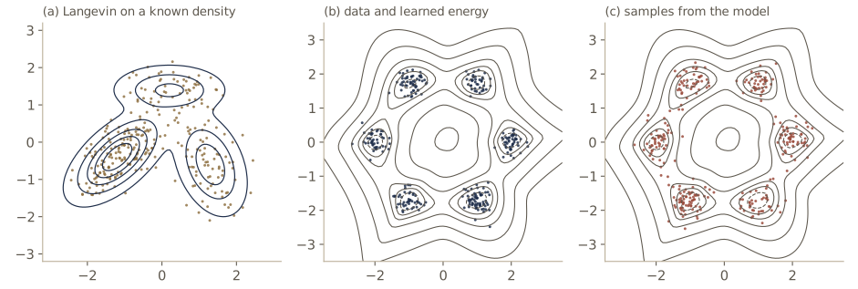
Training an energy network. We put the pieces together. The data are our own: 2,000 points in six tight clusters on a circle of radius 2, which is hard for any single simple density but easy to see. The energy is a small multilayer perceptron with two hidden layers of 64 SiLU units. Each training step:
- takes a minibatch of data points (the positive phase);
- generates the same number of negative samples by running a few steps of Langevin dynamics on the current energy, using autograd for \(\nabla_{\mathbf{x}} E\);
- minimizes \(\text{mean}\, E(\text{data}) - \text{mean}\, E(\text{negatives})\), whose gradient is the negative of the likelihood gradient above, with Adam.
Running every chain to equilibrium at every step is out of the question, so we use contrastive divergence (Hinton, 2002): start each chain at a training point and run only a few steps. The chains cannot wander far, which makes them cheap, but it also means the energy is only shaped near the data; a region far from any data point that the model wrongly favors may never be visited by a negative chain and so never corrected. Hinton’s original proposal used as little as one step of Gibbs sampling. We use 20 Langevin steps of size 0.01, enough to move a sample by about 0.6, well beyond the width of a cluster. Two details keep training stable. The negatives are detached from the parameter graph, so gradients flow only through \(E(\mathbf{x}, \mathbf{w})\) at fixed \(\mathbf{x}\), as the formula says. And a small penalty \(\alpha\, (E_+^2 + E_-^2)\) on the energy values stops the energy from drifting to huge magnitudes, a common regularizer in energy-based training that does not change which shape is preferred.
def make_ring(N, rng, K=6, radius=2.0, sd=0.2):
    k = rng.integers(0, K, N)
    angle = 2 * np.pi * k / K
    centers = radius * np.stack([np.cos(angle), np.sin(angle)], axis=1)
    return centers + sd * rng.standard_normal((N, 2))

def ring_log_density(X, K=6, radius=2.0, sd=0.2):
    angle = 2 * np.pi * np.arange(K) / K
    C = radius * np.stack([np.cos(angle), np.sin(angle)], axis=1)
    d2 = np.sum((X[:, None, :] - C[None]) ** 2, axis=2)
    return logsumexp(-d2 / (2 * sd ** 2), axis=1) - np.log(K) - np.log(2 * np.pi * sd ** 2)

class EnergyNet(torch.nn.Module):
    """E(x, w): a small MLP from R^2 to one scalar per point."""
    def __init__(self, H=64):
        super().__init__()
        self.net = torch.nn.Sequential(torch.nn.Linear(2, H), torch.nn.SiLU(),
                                       torch.nn.Linear(H, H), torch.nn.SiLU(),
                                       torch.nn.Linear(H, 1))

    def forward(self, x):
        return self.net(x).squeeze(-1)

def langevin_torch(E, x, eta, T, gen):
    """Langevin dynamics on exp(-E): x <- x - eta grad_x E + sqrt(2 eta) eps."""
    x = x.detach().clone()
    for _ in range(T):
        x.requires_grad_(True)
        grad_x, = torch.autograd.grad(E(x).sum(), x)     # score = -grad_x E
        x = (x - eta * grad_x + np.sqrt(2 * eta) * torch.randn(x.shape, generator=gen)).detach()
    return x

X_train = make_ring(2000, rng)
X_test = make_ring(1000, rng)
print("data:", X_train.shape, " true mean ln p on test data:",
      f"{ring_log_density(X_test).mean():.3f}")
data: (2000, 2) true mean ln p on test data: -1.432
def train_ebm(X, n_iter=1000, B=200, T_steps=20, eta=0.01, alpha=0.1, lr=1e-3, seed=14):
    torch.manual_seed(seed)
    gen = torch.Generator().manual_seed(seed)
    E = EnergyNet()
    opt = torch.optim.Adam(E.parameters(), lr=lr)
    X = torch.tensor(X, dtype=torch.float32)
    for it in range(1, n_iter + 1):
        x_pos = X[torch.randint(0, len(X), (B,), generator=gen)]
        x_neg = langevin_torch(E, x_pos, eta, T_steps, gen)      # contrastive divergence
        E_pos, E_neg = E(x_pos), E(x_neg)
        loss = E_pos.mean() - E_neg.mean() + alpha * (E_pos ** 2 + E_neg ** 2).mean()
        opt.zero_grad()
        loss.backward()
        opt.step()
        if it % 200 == 0:
            print(f"step {it:4d}: mean E(data) {E_pos.mean().item():7.3f}"
                  f"   mean E(negatives) {E_neg.mean().item():7.3f}")
    return E, gen

E_net, gen = train_ebm(X_train)
step  200: mean E(data)  -0.141   mean E(negatives)   0.177
step  400: mean E(data)  -0.143   mean E(negatives)   0.069
step  600: mean E(data)  -0.139   mean E(negatives)   0.220
step  800: mean E(data)  -0.343   mean E(negatives)   0.287
step 1000: mean E(data)  -0.351   mean E(negatives)   0.162
The negatives keep a higher average energy than the data. With exact model samples and no penalty, the two phases would balance at a maximum of the likelihood; with short chains started at the data and the energy penalty, the fixed point is shifted, and the energies do not settle to equal values. Neither the energies nor the loss tell us whether the model is good. Because we are in two dimensions we can cheat: evaluate \(\exp(-E)\) on a fine grid, sum to get \(Z(\mathbf{w})\), and compute an exact test log-likelihood. As reference points we use the true density and a single Gaussian fitted by maximum likelihood.
g = np.linspace(-4.5, 4.5, 301)
dg = g[1] - g[0]
grid_pts = torch.tensor(np.stack(np.meshgrid(g, g), axis=-1).reshape(-1, 2), dtype=torch.float32)
with torch.no_grad():
    E_grid = E_net(grid_pts).double().numpy()
    E_test = E_net(torch.tensor(X_test, dtype=torch.float32)).double().numpy()
ln_Z = logsumexp(-E_grid) + 2 * np.log(dg)                   # quadrature for the partition function
mu_g, S_g = X_train.mean(axis=0), np.cov(X_train.T, bias=True)
d = X_test - mu_g
ll_gauss = (-0.5 * np.sum(d @ np.linalg.inv(S_g) * d, axis=1)
            - 0.5 * np.log(np.linalg.det(2 * np.pi * S_g)))           # fitted Gaussian
print(f"mean test ln p:  EBM {np.mean(-E_test - ln_Z):.3f}   single Gaussian {ll_gauss.mean():.3f}"
      f"   true density {ring_log_density(X_test).mean():.3f}")
mean test ln p: EBM -1.631 single Gaussian -3.556 true density -1.432
The energy model is about 1.9 nats per point better than the Gaussian and about 0.2 nats below the true density, after a thousand steps of training on one CPU thread (about 15 seconds). More iterations, a larger batch, and a GPU would close more of the gap. To generate new points, we run long Langevin chains on the trained energy starting from uniform noise over the square \([-3.5, 3.5]^2\), far from any data, and check where they end up:
x0 = -3.5 + 7 * torch.rand((600, 2), generator=gen)
x_gen = langevin_torch(E_net, x0, 0.01, 500, gen).numpy()
radius = np.linalg.norm(x_gen, axis=1)
angle = np.mod(np.arctan2(x_gen[:, 1], x_gen[:, 0]) + np.pi / 6, 2 * np.pi)
print(f"radius: mean {radius.mean():.3f}, sd {radius.std():.3f}  (data: 2.0 and about 0.2)")
print("samples per cluster:", np.bincount((angle // (np.pi / 3)).astype(int), minlength=6))
radius: mean 2.018, sd 0.252  (data: 2.0 and about 0.2)
samples per cluster: [ 97  91  89  89 129 105]
The samples lie on the ring and cover all six clusters in roughly equal numbers, as the data do. The figure above shows the learned energy and these samples.
Watch out. Short-run chains are an approximation, and it is easy to fool yourself. Contrastive divergence does not follow the likelihood gradient exactly, and a model trained with very short chains can be good near the data yet put spurious low-energy regions elsewhere, which long-run sampling then finds. Always check a trained energy model by sampling from it with chains that start far from the data, as we did, and in low dimensions by normalizing it on a grid. Exercise 9 asks you to shorten the chains and see what breaks.
In practice. On images, the same recipe needs more machinery: larger networks, a persistent buffer of past negatives from which chains are restarted (so that they effectively run much longer than a few steps), careful step sizes and noise levels, and a GPU. Budget it accordingly: every training step costs \(T\) extra forward and backward passes. The score-based view offers a way out of the negative phase altogether. Score matching trains a network to output \(\nabla_{\mathbf{x}} \ln p\) directly, with no partition function and no model samples during training, and Langevin dynamics then generates samples from the learned score. With noise added at many scales, that is the score-based diffusion model of module 20.
A final remark on names. Langevin updates also appear with the roles of \(\mathbf{x}\) and \(\mathbf{w}\) swapped: stochastic gradient Langevin dynamics (Welling and Teh, 2011) adds \(\sqrt{2\eta}\)-scaled noise to minibatch gradient steps on the log posterior over the weights, turning stochastic gradient training into approximate posterior sampling for Bayesian neural networks. The mathematics is the same; only the variable being sampled changes.
Summary
| Method | What it needs | What it gives | Key property |
|---|---|---|---|
| Monte Carlo average | independent samples from \(p\) | unbiased \(\mathbb{E}[f]\) | error \(\sqrt{\operatorname{var}[f]/L}\), independent of dimension |
| Inverse CDF, Box–Muller, Cholesky | a CDF to invert, or a Gaussian | exact samples | \(y = h^{-1}(z)\); \(\mathbf{y} = \boldsymbol{\mu} + \mathbf{L}\mathbf{z}\) |
| Rejection sampling | \(\widetilde{p}\), proposal \(q\), bound \(kq \geq \widetilde{p}\) | exact samples | acceptance \(Z_p/k\), exponentially small in \(D\) |
| Adaptive rejection | log-concave \(\widetilde{p}\) and its derivative | exact samples | tangent envelope refined at rejected points |
| Importance sampling | \(\widetilde{p}\), proposal \(q\) | weighted estimates, \(Z_p/Z_q\) | \(w_l \propto \widetilde{p}/\widetilde{q}\); \(L_{\text{eff}} = 1/\sum_l w_l^2\) collapses with mismatch and \(D\) |
| SIR | as importance sampling | approximate samples | resample with probabilities \(w_l\); exact as \(L \to \infty\) |
| Metropolis–Hastings | \(\widetilde{p}\), any proposal | correlated samples | accept \(\min\left(1, \frac{\widetilde{p}(\mathbf{z}^{\star}) q(\mathbf{z} \mid \mathbf{z}^{\star})}{\widetilde{p}(\mathbf{z}) q(\mathbf{z}^{\star} \mid \mathbf{z})}\right)\); detailed balance |
| Gibbs sampling | conditionals \(p(z_i \mid \mathbf{z}_{\setminus i})\) | correlated samples | MH with acceptance 1; \(\tau_{\text{int}} = (1+r^2)/(1-r^2)\) for a correlated Gaussian |
| Ancestral / likelihood weighting | a directed graph | exact samples / weighted posterior | parents first; weight = product of clamped factors |
| Langevin dynamics | the score \(\nabla_{\mathbf{x}} \ln p = -\nabla_{\mathbf{x}} E\) | approximate samples | \(\mathbf{x} \leftarrow \mathbf{x} + \eta \nabla_{\mathbf{x}} \ln p + \sqrt{2\eta}\,\boldsymbol{\epsilon}\); bias \(O(\eta)\) |
| EBM maximum likelihood | data and model samples | trained \(E(\mathbf{x}, \mathbf{w})\) | gradient \(= -\mathbb{E}_{p_{\mathrm{D}}}[\nabla_{\mathbf{w}} E] + \mathbb{E}_{p_{\mathrm{M}}}[\nabla_{\mathbf{w}} E]\) |
Ideas to carry forward:
- Monte Carlo error depends on the variance of what we average, not on the dimension. Methods that draw from a fixed proposal (rejection, importance) pay for dimension through the proposal mismatch, which grows exponentially; report acceptance rates and effective sample sizes to see it.
- MCMC replaces independence by a chain whose equilibrium is the target. Detailed balance is the usual way to guarantee the right equilibrium; the autocorrelation time tells us what the samples are worth, and random-walk behavior makes it grow like the squared ratio of the largest to the smallest length scale.
- The normalizing constant drops out of every method here: out of rejection and MH ratios, out of self-normalized weights, and out of the score. That is why energy-based models, which never compute \(Z(\mathbf{w})\), can still be trained and sampled.
- Training an energy model balances a positive phase on data against a negative phase on the model’s own samples. The score \(\nabla_{\mathbf{x}} \ln p\) that drives Langevin sampling is the object that diffusion models learn directly.
Exercises
- Show that the Monte Carlo estimator is unbiased and derive its variance \(\operatorname{var}[f]/L\). Then suppose the samples come from a stationary chain with autocorrelations \(\rho_k\); show that for large \(L\) the variance is approximately \(\tau_{\text{int}} \operatorname{var}[f]/L\) and check the formula with the Gibbs chains of the notes.
- The logistic density has CDF \(\sigma(y)\). Derive its inverse-CDF sampler, implement it, and check the variance against \(\pi^2/3\). Then use the inverse-CDF method on a grid, as in the energy-based model check, to sample the bimodal target \(\widetilde{p}\) of the rejection-sampling section and compare its KS distance with that of rejection sampling at equal cost.
- Derive the within-piece inverse CDF \(z = t + s^{-1}\ln\{w + v(1 - w)\}\) used by
ars, for both signs of the slope, and the log-mass of a piece. Add a lower “squeeze” function (the chords between consecutive hull points) that accepts most proposals without evaluating \(h\), and count how many evaluations of \(h\) it saves. - For \(p = \mathcal{N}(\mathbf{0}, \mathbf{I})\) and \(q = \mathcal{N}(\mathbf{0}, s^2\mathbf{I})\) in \(D\) dimensions, show that \(\mathbb{E}_q[(p/q)^2] = \{s^2/\sqrt{2s^2 - 1}\}^D\). What happens for \(s^2 \leq 1/2\), and what does that say about proposals with lighter tails than the target? Demonstrate it numerically in one dimension.
- Show that the Gibbs sampler with a random choice of variable at each step satisfies detailed balance, while the systematic sweep in general does not. Check both statements on a small discrete joint distribution over two binary variables by building the transition matrices.
- Construct a distribution on two variables for which Gibbs sampling is not ergodic, for example a uniform density on two squares that touch only at a corner. Run
gibbs-style updates from each square and report what fraction of time the chain spends in each. - Implement the Metropolis-adjusted Langevin algorithm: use the Langevin update as a proposal \(q(\mathbf{x}^{\star} \mid \mathbf{x}) = \mathcal{N}(\mathbf{x} + \eta\nabla \ln p(\mathbf{x}), 2\eta\mathbf{I})\) and accept with the Metropolis–Hastings rule. Show that it removes the variance inflation \(1/(1 - \eta/2)\) for the standard Gaussian, and compare its autocorrelation time with random-walk Metropolis on the ridge target at matched acceptance rates.
- Starting from \(Z(\mathbf{w}) = \int \exp\{-E(\mathbf{x}, \mathbf{w})\}\, \mathrm{d}\mathbf{x}\), derive \(\nabla_{\mathbf{w}} \ln Z = -\mathbb{E}_{p_{\mathrm{M}}}[\nabla_{\mathbf{w}} E]\) and show also that \(\nabla_{\mathbf{w}}^2 \ln Z\) is a covariance matrix. What does that imply about the convexity of the negative log-likelihood when \(E\) is linear in \(\mathbf{w}\)?
- Retrain the energy network with 2 Langevin steps per negative instead of 20, and with 20 steps but chains started from uniform noise instead of from the data. For each, report the grid-normalized test log-likelihood and the long-run samples. Which variant puts mass in the wrong places, and why?
- Replace the ring data by a two-dimensional distribution of your own with a hole or a thin curve (a spiral, two interleaved crescents). Train the energy network, and plot the learned density next to a kernel density estimate with a tuned bandwidth. Where does each do better?
- In your own words: why does the partition function disappear from the Metropolis acceptance ratio, from self-normalized importance weights, and from Langevin dynamics, but not from the likelihood gradient of an energy-based model? Explain how the negative phase deals with it.
Going further
- Bishop & Bishop, chapter 14 — the source for this module. Exercises 14.1–14.2 (the Monte Carlo estimator), 14.3–14.6 (transformations, Box–Muller, Cholesky), 14.7–14.10 (rejection and adaptive rejection sampling), 14.11–14.14 (random walks, Gibbs sampling, over-relaxation), 14.15 (likelihood weighting), and 14.16–14.18 (energy-based models) extend the material here.
- Intro to ML, module 11 — the same material at greater length from PRML, plus slice sampling, Hamiltonian Monte Carlo, and estimating partition functions. Module 11 of this course covers the graphs behind ancestral sampling, and module 20 takes the score and Langevin dynamics into diffusion models.
- W. Keith Hastings, “Monte Carlo sampling methods using Markov chains and their applications”, Biometrika, 1970 — the Metropolis–Hastings algorithm.
- Radford M. Neal, Probabilistic Inference Using Markov Chain Monte Carlo Methods, technical report CRG-TR-93-1, University of Toronto, 1993 — a thorough review of MCMC, including ergodicity and the scaling of random-walk methods.
- Geoffrey E. Hinton, “Training products of experts by minimizing contrastive divergence”, Neural Computation, 2002 — contrastive divergence.
- Yang Song and Diederik P. Kingma, “How to train your energy-based models”, 2021 — a survey of maximum likelihood with MCMC, score matching, and noise-contrastive methods for energy-based models.
These notes follow the chapters of C. M. Bishop and H. Bishop, Deep Learning: Foundations and Concepts (Springer, 2024), the course text, which the authors make free to read online. The explanations, code, figures, and exercises here are written for this course; the book remains the reference, with the full derivations and many more exercises.