CSE 676 · Module 09 · Week 5
Regularization
Inductive bias, invariance and equivariance, weight decay, early stopping and double descent, parameter sharing, residual connections, model averaging, and dropout.
Companion reading: Bishop & Bishop, Deep Learning: Foundations and Concepts, chapter 9, “Regularization”
By the end of this module you can
- Explain why learning from finite data is an ill-posed inverse problem, state the no free lunch theorem carefully, and describe what an inductive bias is.
- Name the four ways of building an invariance into a model, show that input noise acts as weight decay for a linear model, and check numerically that a convolution is translation equivariant while a dense layer is not.
- Derive weight decay from a Gaussian prior, describe its effect along the eigenvectors of the Hessian, compute the effective number of parameters, and build a regularizer that is consistent under linear rescaling of inputs and targets.
- Explain why an L1 penalty produces exact zeros while an L2 penalty only shrinks, and show it with coefficient paths.
- Use learning curves to stop training early, relate the number of steps to a weight-decay coefficient, and reproduce double descent with random-feature least squares.
- Implement hard and soft weight sharing and verify the gradients of the mixture-of-Gaussians prior against autograd.
- Explain why deep plain stacks are hard to train, build residual networks, and read them as ensembles of paths and as discretized differential equations.
- Analyze committees and bagging, implement inverted dropout and check it against
nn.Dropout, and use Monte Carlo dropout for a predictive spread.
Contents
- Inductive bias
- Weight decay
- Learning curves
- Parameter sharing
- Residual connections
- Model averaging
- Summary
- Exercises
- Going further
In module 07 and module 08 we learned how to make the training error of a deep network small. That is only half of the job. A network with a few hundred thousand parameters can fit a training set of a thousand images perfectly, including every mislabeled one, and still predict badly on the next image it sees. What we want is small error on data the network has not seen, and the techniques that trade some training error for better generalization are collectively called regularization.
The simplest regularizer is one we met with polynomial curve fitting in Intro to ML, module 03: add a penalty on the size of the weights,
\[\widetilde{E}(\mathbf{w}) = E(\mathbf{w}) + \frac{\lambda}{2}\mathbf{w}^{\mathrm{T}}\mathbf{w},\]where \(E(\mathbf{w})\) is the unregularized error and the regularization coefficient \(\lambda\) sets the strength of the penalty. In the language of the bias–variance decomposition, the penalty lowers the variance of the fitted model at the price of some bias. This module takes a much wider view. We start from the question of why any learning is possible at all (the answer is inductive bias), then look at the tools deep learning uses in practice: weight decay and its variants, early stopping, the surprising double-descent behavior of very large models, parameter sharing, residual connections, ensembles, and dropout. Several of these are routinely used together; a network trained with weight decay and dropout and stopped early is ordinary practice.
Two themes run through the module. First, a regularizer is a statement of prior knowledge, and the best regularizers encode something true about the problem (smoothness, a symmetry). Second, in deep learning much of the regularization is implicit: it comes from the architecture and from the optimizer rather than from a penalty term. All experiments are small enough to run on a laptop CPU in a couple of minutes; with a GPU you can scale the MNIST experiments to the full training set and larger networks by changing a few numbers.
We use NumPy for the closed-form experiments and PyTorch for everything that trains a network. As always, every random number comes from a seeded generator so that the outputs below repeat exactly.
import copy
import itertools
import warnings

import numpy as np
import torch
import torch.nn as nn
import torch.nn.functional as F
from torchvision import datasets

warnings.filterwarnings("ignore", category=FutureWarning)   # quiet a torch.func notice
np.set_printoptions(precision=4, suppress=True)
rng = np.random.default_rng(9)
torch.manual_seed(9)
Inductive bias
When we fit polynomials of increasing order to a few noisy points, the best predictions came from an intermediate order: a straight line could not follow the data, and a ninth-order polynomial followed the noise. The same happened when we fixed the order and varied \(\lambda\). The bias–variance decomposition explained why: some bias is needed to generalize from a finite sample, and the right amount shrinks as the data set grows. We ignore practical constraints such as memory and speed here and focus on predictive accuracy alone.
Inverse problems
Most learning tasks are inverse problems. The forward direction is easy: given a conditional distribution \(p(t \mid \mathbf{x})\) and some inputs, we can sample targets. Learning runs the other way. We see finitely many pairs \((\mathbf{x}_n, t_n)\) and must infer a whole distribution, or at least a whole function, from them. That problem is ill-posed: infinitely many distributions assign nonzero density to the observed targets, so the data alone never single out one answer.
Here is the ill-posedness in its most concrete form. We fit a polynomial with ten coefficients through six points. The design matrix has a four-dimensional null space, so we can add any null-space vector to a solution without changing its fit to the training data, and yet the predictions between and beyond the points change.
x_tr = np.linspace(-1, 1, 6)
t_tr = np.sin(np.pi * x_tr) + rng.normal(0, 0.1, 6)

def poly(x, M=10):
    """Design matrix with columns 1, x, ..., x^(M-1)."""
    return np.vander(x, M, increasing=True)

Phi = poly(x_tr)
w_min = np.linalg.lstsq(Phi, t_tr, rcond=None)[0]     # minimum-norm interpolant
null_basis = np.linalg.svd(Phi)[2][6:]                # rows span {v : Phi v = 0}
w_other = w_min + null_basis.T @ rng.normal(0, 10.0, 4)
x_new = np.array([-1.1, -0.5, 0.1, 0.7])
for name, w in [("minimum norm ", w_min), ("plus null vec", w_other)]:
    print(f"{name}: max train residual {np.abs(Phi @ w - t_tr).max():.1e}"
          f"   predictions {np.round(poly(x_new) @ w, 3)}")
minimum norm : max train residual 1.9e-15   predictions [-1.804 -1.113  0.307  0.779]
plus null vec: max train residual 3.6e-15   predictions [-0.116 -1.094  0.325  1.041]
Both coefficient vectors fit the six points to machine precision. Away from the points they disagree, strongly outside the data range (at \(x = -1.1\)) and noticeably inside it (at \(x = 0.7\)), and nothing in the data says which one is right. To predict at all we must prefer some solutions over others. That preference is called the inductive bias of the learner (or its prior knowledge). The minimum-norm solution in the first row is itself a choice: it is what weight decay picks in the limit \(\lambda \to 0\).
Good inductive biases come from what we know about the problem. In most applications small changes of the input should cause small changes of the output, so we prefer smooth functions; a penalty on \(\lVert \mathbf{w} \rVert^2\) pushes toward functions that change slowly with the input. When recognizing objects in images, the identity of an object does not depend on where it sits in the frame; building in this translation invariance makes the learning problem far easier, which is the story of module 10. A wrong bias hurts: assuming a linear relation when the truth is strongly nonlinear gives a model that is confidently inaccurate.
Transfer learning and multi-task learning also fit this picture. When labeled data for our task are scarce, we train on a related task as well and let the two share most of the network. The assumption that the tasks need similar internal features is an inductive bias, a richer one than a penalty on weight size, and it explains why the extra data help (Bishop & Bishop §6.3.4).
The no free lunch theorem
Deep networks are flexible enough that one might hope for a universal learner, one that is best for every problem. The no free lunch theorem (Wolpert, 1996) rules this out. In one standard form: consider a finite input space and a fixed training set, and measure accuracy only on inputs outside the training set. If every possible target function is equally likely a priori, then every learning algorithm has the same expected off-training-set accuracy. An algorithm that does better than average on some target functions must do worse on others.
For binary labels on a finite domain the argument fits in one line: under a uniform prior over functions, the labels at test inputs are independent of the labels at training inputs, so no rule that looks at the training labels can predict the test labels better than a coin. We can check this by enumeration. With three binary inputs there are \(2^8 = 256\) target functions. We train on four of the eight inputs, test on the other four, and compare three learners: one nearest neighbor (in Hamming distance), a “contrarian” that predicts the opposite of nearest neighbor, and a constant.
inputs = list(itertools.product([0, 1], repeat=3))         # the 8 possible inputs
train_ids, test_ids = [0, 3, 5, 6], [1, 2, 4, 7]

def nearest_neighbor(train_x, train_t, x):
    dist = [sum(a != b for a, b in zip(x, u)) for u in train_x]
    return train_t[int(np.argmin(dist))]

def contrarian(train_x, train_t, x):
    return 1 - nearest_neighbor(train_x, train_t, x)

def constant(train_x, train_t, x):
    return 0

def off_training_accuracy(learner, f):
    """f is a tuple of 8 labels, one per input."""
    train_x = [inputs[i] for i in train_ids]
    train_t = [f[i] for i in train_ids]
    return np.mean([learner(train_x, train_t, inputs[i]) == f[i] for i in test_ids])

all_functions = list(itertools.product([0, 1], repeat=8))
# a "structured" family: functions of a single bit, and majority vote, with their negations
structured = [tuple(x[k] ^ neg for x in inputs) for k in range(3) for neg in (0, 1)]
structured += [tuple(int(sum(x) >= 2) ^ neg for x in inputs) for neg in (0, 1)]
for learner in [nearest_neighbor, contrarian, constant]:
    acc_all = np.mean([off_training_accuracy(learner, f) for f in all_functions])
    acc_str = np.mean([off_training_accuracy(learner, f) for f in structured])
    print(f"{learner.__name__:17s} all 256 functions {acc_all:.3f}"
          f"   structured family {acc_str:.3f}")
nearest_neighbor  all 256 functions 0.500   structured family 0.750
contrarian        all 256 functions 0.500   structured family 0.250
constant          all 256 functions 0.500   structured family 0.500
Averaged over all 256 functions, all three learners score exactly one half. On the structured family, where nearby inputs tend to share a label, nearest neighbor wins and the contrarian loses by the same margin. That is the practical message. The theorem is a statement about averages over all conceivable problems, most of which look like noise and never arise in practice. Real problems have structure, above all smoothness, and learners whose inductive bias matches that structure do well across a very wide range of applications.
What the theorem does make clear is that there is no learning “purely from data”. Bias can be implicit: a network with a finite number of parameters can only represent some functions, and, as we will see, gradient descent itself prefers some solutions. It can also be explicit, through the choice of model, a penalty term, or the architecture. The model-based view of machine learning argues for making all of these assumptions explicit so they can be chosen deliberately (Bishop & Bishop §9.1.2 gives a reference). Part of the craft of deep learning is designing the inductive bias well.
Symmetry and invariance
Many predictions should not change when the input is transformed in certain ways. A photograph of a dog is a dog wherever it sits in the frame (translation invariance) and whatever its size (scale invariance). Exploiting such symmetries is the theme of geometric deep learning.
The transformations that express a symmetry form a group: a set of elements with a composition \(A \circ B\) that is closed (composing two elements gives an element of the set), associative, has an identity element \(I\) with \(A \circ I = I \circ A = A\), and gives every element an inverse \(A^{-1}\) with \(A \circ A^{-1} = A^{-1} \circ A = I\). The cyclic shifts of a 28-pixel row form a group of 28 elements (a shift by \(k\) composed with a shift by \(m\) is a shift by \(k + m\) modulo 28, and the inverse of a shift by \(k\) is a shift by \(-k\)); the translations of the plane form a continuous group.
In principle a network could learn an invariance from data alone. In practice this is expensive: shifting a digit by two pixels changes most of its pixel values, and real problems need invariance to shifts, scalings, rotations, brightness, and more at the same time, so the number of combinations that would have to appear in the training set explodes. There are four more economical routes:
- Pre-processing. Compute features that are unchanged by the transformations and feed only those to the model. The difficulty is to remove the nuisance variation without removing useful information, and hand-designed features have largely been replaced by learned ones.
- A regularized error function. Add a penalty that grows when the output changes under the transformation. Tangent propagation, below, is the standard example.
- Data augmentation. Enlarge the training set with transformed copies of the training inputs, keeping their targets.
- Architecture. Build the invariance into the network’s structure, as convolutional networks do for translations.
Tangent propagation
Let \(\mathbf{s}(\mathbf{x}, \xi)\) be the input transformed by an amount \(\xi\), with \(\mathbf{s}(\mathbf{x}, 0) = \mathbf{x}\). For a small transformation the input moves along the tangent vector \(\boldsymbol{\tau}_n = \partial \mathbf{s}(\mathbf{x}_n, \xi) / \partial \xi\) at \(\xi = 0\), and by the chain rule the output changes at the rate \(\mathbf{J}_n \boldsymbol{\tau}_n\), where \(\mathbf{J}_n\) is the Jacobian of the outputs with respect to the inputs. Tangent propagation adds the penalty
\[\Omega = \frac{1}{2}\sum_{n} \lVert \mathbf{J}_n \boldsymbol{\tau}_n \rVert^2,\]which is zero exactly when the outputs are locally invariant. In PyTorch the product \(\mathbf{J}\boldsymbol{\tau}\) is a Jacobian–vector product, which forward-mode differentiation computes at about the cost of one forward pass. For a horizontal shift of an image, the tangent vector is minus the horizontal derivative of the image, which a central difference approximates.
def tangent_prop_penalty(model, X, tau):
    """0.5 * sum_n ||J_n tau_n||^2 via a Jacobian-vector product (forward mode)."""
    _, Jtau = torch.func.jvp(model, (X,), (tau,))
    return 0.5 * (Jtau ** 2).sum()

train = datasets.MNIST(root="data", train=True, download=True)
X_img = train.data[:6000].float().div(255.)          # (6000, 28, 28)
y_all = train.targets[:6000]

imgs = X_img[:8]
# shifting right by xi: s(x, xi)[u, v] = x[u, v - xi], so ds/dxi = -dx/dv
tau = (torch.roll(imgs, 1, dims=2) - torch.roll(imgs, -1, dims=2)) / 2
torch.manual_seed(0)
net = nn.Sequential(nn.Flatten(), nn.Linear(784, 64), nn.Tanh(), nn.Linear(64, 10))
omega = tangent_prop_penalty(net, imgs, tau)
omega.backward()                             # differentiable, so it can be trained on
Jtau = torch.func.jvp(net, (imgs,), (tau,))[1]
eps = 1e-3                                   # check J tau by central differences
with torch.no_grad():
    fd = (net(imgs + eps * tau) - net(imgs - eps * tau)) / (2 * eps)
print(f"penalty {omega.item():.4f}   max |J tau - finite difference| "
      f"{(Jtau - fd).abs().max().item():.1e}")
penalty 0.0880 max |J tau - finite difference| 3.1e-05
The penalty is a differentiable function of the weights, so we can add it to the error and train. Its limitation is that it only enforces invariance to infinitesimal transformations, and it adds a Jacobian–vector product to every step.
Data augmentation and its hidden regularizer
Data augmentation is usually the easiest route. With stochastic gradient descent we transform each mini-batch afresh, drawing a new random transformation every time an example is revisited; for batch methods we would instead replicate each point several times and transform each copy. Typical image augmentations are flips, crops and shifts, small rotations and scalings, brightness and contrast changes, added noise, and color shifts, and for medical images of soft tissue, smooth elastic deformations.
Augmentation with small transformations is secretly a regularizer. Expanding the error to second order in the size of the transformation gives the original error plus a penalty on the derivative of the output along the transformation direction, which is closely related to tangent propagation. The simplest case is augmentation by additive input noise, and for a linear model the result is exact. Take \(y(\mathbf{x}, \mathbf{w}) = w_0 + \mathbf{w}^{\mathrm{T}}\mathbf{x}\) and add independent noise \(\boldsymbol{\epsilon}\) with zero mean and covariance \(\sigma^2\mathbf{I}\) to each input. Then
\[\begin{aligned} \mathbb{E}_{\boldsymbol{\epsilon}}\left[ \left( w_0 + \mathbf{w}^{\mathrm{T}}(\mathbf{x}_n + \boldsymbol{\epsilon}) - t_n \right)^2 \right] &= \left( w_0 + \mathbf{w}^{\mathrm{T}}\mathbf{x}_n - t_n \right)^2 + 2\left( w_0 + \mathbf{w}^{\mathrm{T}}\mathbf{x}_n - t_n \right)\mathbf{w}^{\mathrm{T}}\mathbb{E}[\boldsymbol{\epsilon}] + \mathbf{w}^{\mathrm{T}}\mathbb{E}[\boldsymbol{\epsilon}\boldsymbol{\epsilon}^{\mathrm{T}}]\mathbf{w} \\ &= \left( w_0 + \mathbf{w}^{\mathrm{T}}\mathbf{x}_n - t_n \right)^2 + \sigma^2 \lVert \mathbf{w} \rVert^2 . \end{aligned}\]Summing over \(n\) with a factor \(\tfrac12\), training on noisy inputs minimizes, on average, the clean sum-of-squares error plus weight decay with \(\lambda = N\sigma^2\), and the bias \(w_0\) is not penalized. We check this by stacking many noisy copies of a small data set and solving ordinary least squares on the stack.
N_lin, D_lin, sigma = 40, 3, 0.5
X_lin = rng.normal(size=(N_lin, D_lin))
t_lin = X_lin @ np.array([1.0, -2.0, 0.5]) + 0.3 + rng.normal(0, 0.2, N_lin)

def with_bias(X):
    return np.hstack([np.ones((len(X), 1)), X])

R = 2000                                            # noisy copies of every point
X_aug = np.tile(X_lin, (R, 1)) + rng.normal(0, sigma, (R * N_lin, D_lin))
w_aug = np.linalg.lstsq(with_bias(X_aug), np.tile(t_lin, R), rcond=None)[0]

A = with_bias(X_lin)
reg = N_lin * sigma**2 * np.diag([0.0, 1.0, 1.0, 1.0])   # lambda = N sigma^2, no bias penalty
w_ridge = np.linalg.solve(A.T @ A + reg, A.T @ t_lin)
print("trained on noisy copies:", w_aug)
print("ridge, lambda = N s^2:  ", w_ridge)
trained on noisy copies: [ 0.2917  0.9446 -1.621   0.5724]
ridge, lambda = N s^2:   [ 0.2871  0.9436 -1.6268  0.5703]
The two agree to within about 0.005, and the remaining gap shrinks as the number of copies grows. For a nonlinear network the same expansion gives, to leading order in \(\sigma^2\), a penalty proportional to \(\sum_n \lVert \partial y / \partial \mathbf{x}_n \rVert^2\), a smoothness penalty known as Tikhonov regularization (Intro to ML, module 05 works through it).
Now augmentation on real images. We take the first 1000 MNIST digits as a training set and 2000 others as a validation set, train the same small multilayer perceptron with and without random shifts of up to three pixels in each direction, and evaluate on the validation images both as they are and randomly shifted. (A multilayer perceptron has no built-in translation invariance, so it is a clean test of what augmentation adds.) The training function below is reused throughout the module. It records the training loss, validation loss, and validation accuracy after every epoch and keeps a copy of the weights with the lowest validation loss, which we need for early stopping later.
X_tr, y_tr = X_img[:1000], y_all[:1000]              # training set
X_va, y_va = X_img[2000:4000], y_all[2000:4000]      # validation set
X_te, y_te = X_img[4000:6000], y_all[4000:6000]      # test set, used only for final numbers

def random_shift(imgs, max_shift, gen):
    """Shift each image cyclically by its own random (dy, dx) in [-max_shift, max_shift]."""
    s = torch.randint(-max_shift, max_shift + 1, (len(imgs), 2), generator=gen)
    return torch.stack([torch.roll(im, (int(a), int(b)), dims=(0, 1))
                        for im, (a, b) in zip(imgs, s)])

def mlp(p_drop=0.0, H=128):
    return nn.Sequential(nn.Flatten(), nn.Linear(784, H), nn.ReLU(), nn.Dropout(p_drop),
                         nn.Linear(H, H), nn.ReLU(), nn.Dropout(p_drop), nn.Linear(H, 10))

def evaluate(model, X, y):
    model.eval()
    with torch.no_grad():
        out = model(X)
    return F.cross_entropy(out, y).item(), (out.argmax(1) == y).float().mean().item()

def train_mnist(model, opt, X, y, epochs, augment=0, seed=0, batch=100):
    """Mini-batch training. Returns the per-epoch history
    (epoch, train loss, val loss, val acc) and (epoch, weights) at the lowest val loss."""
    gen = torch.Generator().manual_seed(seed)
    history, best = [], (float("inf"), 0, None)
    for epoch in range(1, epochs + 1):
        model.train()                                 # dropout on (if any)
        perm = torch.randperm(len(X), generator=gen)
        for i in range(0, len(X), batch):
            idx = perm[i:i + batch]
            xb = random_shift(X[idx], augment, gen) if augment else X[idx]
            loss = F.cross_entropy(model(xb), y[idx])
            opt.zero_grad()
            loss.backward()
            opt.step()
        train_loss, _ = evaluate(model, X, y)
        val_loss, val_acc = evaluate(model, X_va, y_va)
        history.append((epoch, train_loss, val_loss, val_acc))
        if val_loss < best[0]:
            best = (val_loss, epoch, copy.deepcopy(model.state_dict()))
    return history, best[1:]

X_va_shift = random_shift(X_va, 3, torch.Generator().manual_seed(1))
for shift in [0, 3]:
    torch.manual_seed(0)
    model = mlp()
    train_mnist(model, torch.optim.Adam(model.parameters(), lr=1e-3), X_tr, y_tr,
                epochs=25, augment=shift)
    acc, acc_shift = evaluate(model, X_va, y_va)[1], evaluate(model, X_va_shift, y_va)[1]
    print(f"max training shift {shift}:  validation accuracy {acc:.3f}"
          f"   on shifted validation images {acc_shift:.3f}")
max training shift 0:  validation accuracy 0.891   on shifted validation images 0.401
max training shift 3:  validation accuracy 0.875   on shifted validation images 0.809
Without augmentation the network is brittle: shifting the validation digits by a few pixels roughly halves its accuracy, because it has only ever seen centered digits. With shifted training copies, the accuracy on shifted digits doubles while the accuracy on centered digits drops by less than two points. Augmentation has taught an invariance that the architecture does not have.
Equivariance
Often we do not want the output to stay fixed under a transformation but to move along with it. If a network \(S\) segments an image \(I\) into foreground and background, then shifting the image should shift the segmentation:
\[S(T(I)) = T(S(I)),\]where \(T\) is the translation. A map with this property is equivariant to \(T\). More generally the transformation on the output side can be a different one, \(S(T(I)) = \widetilde{T}(S(I))\): if the segmentation has a lower resolution than the image, \(\widetilde{T}\) is the corresponding smaller shift, and if \(S\) reports the orientation of an object, a rotation \(T\) of the image (a complicated change of every pixel) corresponds to adding a constant to one number. Invariance is the special case in which \(\widetilde{T}\) is the identity: a classifier \(C\) with \(C(T(I)) = C(I)\).
A convolution is translation equivariant by construction: it applies the same small filter at every position, so shifting the input shifts the output. A dense layer has a separate weight for every input–output pair and has no reason to commute with shifts. We check both on an MNIST digit, using cyclic shifts and circular padding so that the image edges do not interfere; averaging the convolution’s output over all positions then gives a translation-invariant feature.
torch.manual_seed(6)
conv = nn.Conv2d(1, 4, kernel_size=5, padding=2, padding_mode="circular", bias=False)
dense = nn.Linear(784, 784, bias=False)

def dense_map(a):
    return dense(a.reshape(len(a), -1)).reshape(len(a), 1, 28, 28)

def T(a):                                     # translate by 3 rows down and 2 columns left
    return torch.roll(a, shifts=(3, -2), dims=(-2, -1))

img = X_img[:1].unsqueeze(1)                  # (1, 1, 28, 28)
with torch.no_grad():
    for name, S in [("convolution", conv), ("dense layer", dense_map)]:
        gap = (S(T(img)) - T(S(img))).abs().max().item()
        print(f"{name}:  max |S(T(I)) - T(S(I))| = {gap:.1e}"
              f"   (size of S(I): {S(img).abs().max().item():.2f})")
    pooled = conv(T(img)).mean(dim=(2, 3)) - conv(img).mean(dim=(2, 3))
    print(f"conv + global average pool:  max change under T = {pooled.abs().max().item():.1e}")
convolution:  max |S(T(I)) - T(S(I))| = 0.0e+00   (size of S(I): 0.75)
dense layer:  max |S(T(I)) - T(S(I))| = 1.0e+00   (size of S(I): 0.69)
conv + global average pool:  max change under T = 3.7e-09
The convolution commutes with the shift exactly, the dense layer does not come close, and pooling over positions turns equivariance into invariance. The figure shows the same thing as pictures.
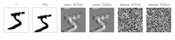
With zero padding instead of circular padding the equivariance holds exactly away from the image border, which is what real convolutional layers give. Module 10 develops this architecture route in full; it is the most powerful of the four, because it enforces the symmetry exactly, costs nothing at training time, and reduces the number of parameters at the same time.
Weight decay
We now return to the explicit penalty \(\tfrac{\lambda}{2}\mathbf{w}^{\mathrm{T}}\mathbf{w}\) and look at it from three sides: as a prior, as a geometric shrinkage along the directions of the Hessian, and as something that has to be set up with care in a network.
A Gaussian prior
Suppose the targets have Gaussian noise with precision \(\beta\) and we place a zero-mean Gaussian prior with precision \(\alpha\) on the weights, \(p(\mathbf{w} \mid \alpha) = \mathcal{N}(\mathbf{w} \mid \mathbf{0}, \alpha^{-1}\mathbf{I})\). The negative log posterior is, up to constants,
\[-\ln p(\mathbf{w} \mid \mathcal{D}) = \beta E(\mathbf{w}) + \frac{\alpha}{2}\mathbf{w}^{\mathrm{T}}\mathbf{w} + \text{const},\]with \(E\) the sum-of-squares error. Dividing by \(\beta\) shows that the most probable weights minimize \(\widetilde{E}\) with \(\lambda = \alpha/\beta\) (Intro to ML, module 03 derives this for linear regression). This gives the penalty a meaning, but also shows its weakness: the prior is placed on the weights, while what we usually know is something about the function the network computes, and the map from weights to functions is too complicated for most such knowledge to be written as a simple weight prior.
The gradient of the regularized error is
\[\nabla \widetilde{E}(\mathbf{w}) = \nabla E(\mathbf{w}) + \lambda \mathbf{w},\](the factor \(\tfrac12\) is there so that the 2 cancels), and one step of gradient descent becomes
\[\mathbf{w} \leftarrow (1 - \eta\lambda)\mathbf{w} - \eta \nabla E(\mathbf{w}).\]Each step first multiplies the weights by a number slightly below one, so weights that the data do not support decay toward zero. That is where the name weight decay comes from.
In PyTorch the weight_decay argument of the optimizers implements this. For plain SGD, and for Adam, it adds \(\lambda\mathbf{w}\) to the gradient, which is exactly the penalty above. AdamW instead applies the multiplicative decay directly to the weights, outside Adam’s per-parameter scaling. That decoupled weight decay is not the same as an L2 penalty once Adam rescales the gradient, and it is the version most modern training recipes use. A single step on a toy model shows the three cases.
def one_step(opt_class, lam, explicit_penalty, **kw):
    torch.manual_seed(1)
    layer = nn.Linear(5, 1)
    x, t = torch.randn(8, 5), torch.randn(8, 1)
    wd = 0.0 if explicit_penalty else lam
    opt = opt_class(layer.parameters(), lr=0.1, weight_decay=wd, **kw)
    loss = F.mse_loss(layer(x), t)
    if explicit_penalty:
        loss = loss + 0.5 * lam * sum((p ** 2).sum() for p in layer.parameters())
    opt.zero_grad()
    loss.backward()
    opt.step()
    return torch.cat([p.detach().ravel() for p in layer.parameters()])

lam = 0.3
for name, opt_class in [("SGD  ", torch.optim.SGD), ("Adam ", torch.optim.Adam),
                        ("AdamW", torch.optim.AdamW)]:
    same = torch.allclose(one_step(opt_class, lam, False), one_step(opt_class, lam, True))
    print(f"{name} weight_decay equals an explicit L2 penalty: {same}")
SGD   weight_decay equals an explicit L2 penalty: True
Adam  weight_decay equals an explicit L2 penalty: True
AdamW weight_decay equals an explicit L2 penalty: False
In practice. Most libraries apply weight decay to every parameter handed to the optimizer, including biases and the scale and shift of normalization layers. Many training recipes exclude those by passing two parameter groups, one with
weight_decayand one without. The next section shows why treating all parameters alike is not ideal.
Shrinkage along the directions of the Hessian
What does the penalty do to the solution? Near a minimum \(\mathbf{w}^{\star}\) of the unregularized error, approximate \(E\) by a quadratic,
\[E(\mathbf{w}) \approx E(\mathbf{w}^{\star}) + \frac{1}{2}(\mathbf{w} - \mathbf{w}^{\star})^{\mathrm{T}}\mathbf{H}(\mathbf{w} - \mathbf{w}^{\star}),\]where \(\mathbf{H}\) is the Hessian at \(\mathbf{w}^{\star}\) (exact for linear regression with a sum-of-squares error). Setting the gradient of \(E + \tfrac{\lambda}{2}\lVert\mathbf{w}\rVert^2\) to zero gives \((\mathbf{H} + \lambda\mathbf{I})\widehat{\mathbf{w}} = \mathbf{H}\mathbf{w}^{\star}\). Write both vectors in the eigenvectors of \(\mathbf{H}\), with \(\mathbf{H}\mathbf{u}_j = \lambda_j \mathbf{u}_j\); because \(\mathbf{H}\) and \(\mathbf{H} + \lambda\mathbf{I}\) share eigenvectors, the equation separates into one equation per direction:
\[\widehat{w}_j = \frac{\lambda_j}{\lambda_j + \lambda}\, w^{\star}_j, \qquad w_j = \mathbf{u}_j^{\mathrm{T}}\mathbf{w}.\]Directions of high curvature (\(\lambda_j \gg \lambda\)), where the error changes quickly and the data pin the weights down, are left almost untouched. Directions of low curvature (\(\lambda_j \ll \lambda\)), where the error barely notices the weight, are pushed nearly to zero. The regularizer suppresses exactly the parameters that matter little for the fit. The sum of the shrinkage factors,
\[\gamma = \sum_j \frac{\lambda_j}{\lambda_j + \lambda},\]counts the directions that survive and is called the effective number of parameters. It falls from the full count at \(\lambda = 0\) to zero as \(\lambda \to \infty\), so tuning \(\lambda\) is a continuous version of choosing how many parameters to use. We verify the per-direction formula for linear regression with strongly correlated inputs, which give a Hessian with widely spread eigenvalues.
N_h, D_h = 50, 6
latent = rng.normal(size=(N_h, 2))
X_h = latent @ rng.normal(size=(2, D_h)) + 0.1 * rng.normal(size=(N_h, D_h))  # correlated
t_h = X_h @ rng.normal(size=D_h) + rng.normal(0, 0.3, N_h)

H = X_h.T @ X_h                                  # Hessian of E = 0.5 ||X w - t||^2
w_star = np.linalg.solve(H, X_h.T @ t_h)
eigvals, U = np.linalg.eigh(H)
lam = 1.0
w_hat = np.linalg.solve(H + lam * np.eye(D_h), X_h.T @ t_h)
print("eigenvalues of H:        ", eigvals)
print("shrinkage w_hat_j / w*_j:", (U.T @ w_hat) / (U.T @ w_star))
print("lambda_j/(lambda_j + lam):", eigvals / (eigvals + lam))
for lam in [0.0, 0.1, 1.0, 10.0, 1000.0]:
    gamma_eff = np.sum(eigvals / (eigvals + lam))
    print(f"lambda = {lam:7.1f}   effective number of parameters {gamma_eff:.2f}")
eigenvalues of H:         [  0.2166   0.3512   0.4832   0.7272  70.8488 526.1632]
shrinkage w_hat_j / w*_j: [0.1781 0.2599 0.3258 0.421  0.9861 0.9981]
lambda_j/(lambda_j + lam): [0.1781 0.2599 0.3258 0.421  0.9861 0.9981]
lambda =     0.0   effective number of parameters 6.00
lambda =     0.1   effective number of parameters 5.17
lambda =     1.0   effective number of parameters 3.17
lambda =    10.0   effective number of parameters 2.03
lambda =  1000.0   effective number of parameters 0.41
The measured shrinkage matches \(\lambda_j/(\lambda_j + \lambda)\) in every direction. Four of the six eigenvalues are small because the inputs are mostly driven by two latent variables, and a coefficient of \(\lambda = 1\) already shrinks those four directions to between a fifth and two fifths of their unregularized size, leaving about three effective parameters.
Consistent regularizers
Plain weight decay has a flaw in networks: it is not compatible with simple rescalings of the data. Consider a two-layer network with hidden units \(z_j = h(\sum_i w_{ji}x_i + w_{j0})\) and linear outputs \(y_k = \sum_j w_{kj}z_j + w_{k0}\). If we transform every input as \(x_i \to \widetilde{x}_i = a x_i + b\) (a change of units, say), the network can compute exactly the same function of the underlying quantity once its first-layer parameters compensate. Substituting \(x_i = (\widetilde{x}_i - b)/a\),
\[\sum_i w_{ji}x_i + w_{j0} = \sum_i \frac{w_{ji}}{a}\widetilde{x}_i + \left( w_{j0} - \frac{b}{a}\sum_i w_{ji} \right),\]so \(\widetilde{w}_{ji} = w_{ji}/a\) and \(\widetilde{w}_{j0} = w_{j0} - (b/a)\sum_i w_{ji}\). Likewise a target transformation \(y_k \to c\,y_k + d\) is absorbed by \(\widetilde{w}_{kj} = c\,w_{kj}\) and \(\widetilde{w}_{k0} = c\,w_{k0} + d\).
Training on the original data and training on the transformed data describe the same problem, so a sensible regularizer should give solutions that are related by exactly these parameter maps. Plain weight decay cannot: it charges \(\widetilde{w}_{ji}^2 = w_{ji}^2/a^2\) at the same rate as before, and it penalizes biases whose values shift. What we need is a penalty that is unchanged by the rescalings, up to a matching change of its coefficients, and that ignores the biases. A separate coefficient per layer, with biases left out, does it:
\[\frac{\lambda_1}{2}\sum_{w \in \mathcal{W}_1} w^2 + \frac{\lambda_2}{2}\sum_{w \in \mathcal{W}_2} w^2,\]where \(\mathcal{W}_1\) and \(\mathcal{W}_2\) are the weights (not the biases) of the two layers. Under the maps above, the first sum is multiplied by \(1/a^2\) and the second by \(c^2\), so the penalty is unchanged if we also set \(\lambda_1 \to a^2\lambda_1\) and \(\lambda_2 \to \lambda_2/c^2\). Here is the check in PyTorch.
def two_layer(M=8):
    return nn.Sequential(nn.Linear(1, M), nn.Tanh(), nn.Linear(M, 1))

def transformed_copy(net, a, b, c, d):
    """Weights that compute c*y(x) + d when the input is a*x + b."""
    new = copy.deepcopy(net)
    L1, L2 = new[0], new[2]
    with torch.no_grad():
        L1.bias -= (b / a) * L1.weight.sum(1)
        L1.weight /= a
        L2.weight *= c
        L2.bias.mul_(c).add_(d)
    return new

def plain_decay(net, lam):
    return 0.5 * lam * sum((p ** 2).sum() for p in net.parameters()).item()

def per_layer_decay(net, lam1, lam2):
    return 0.5 * (lam1 * (net[0].weight ** 2).sum() + lam2 * (net[2].weight ** 2).sum()).item()

torch.manual_seed(2)
net = two_layer()
a, b, c, d = 1.8, 32.0, 0.5, -3.0                    # e.g. Celsius -> Fahrenheit inputs
new = transformed_copy(net, a, b, c, d)
x = torch.linspace(-2, 2, 5).unsqueeze(1)
with torch.no_grad():
    same = torch.allclose(new(a * x + b), c * net(x) + d, atol=1e-5)
print(f"transformed network computes c*y(x) + d on inputs a*x + b: {same}")
print(f"plain weight decay:  {plain_decay(net, 0.1):.4f} -> {plain_decay(new, 0.1):.4f}")
print(f"per-layer, rescaled: {per_layer_decay(net, 0.1, 0.1):.4f} -> "
      f"{per_layer_decay(new, 0.1 * a**2, 0.1 / c**2):.4f}")
transformed network computes c*y(x) + d on inputs a*x + b: True
plain weight decay:  0.1615 -> 17.7421
per-layer, rescaled: 0.0739 -> 0.0739
The transformed network is an exact copy in new units, yet plain weight decay assigns it a very different penalty, so it would steer training toward a different solution. The per-layer penalty with rescaled coefficients gives the same value. Intro to ML, module 05 goes one step further and shows that retraining moves the solution under plain weight decay but not under the consistent one.
In practice. The cheapest defense is to standardize inputs (and regression targets) to zero mean and unit variance before training. Then the question of units disappears, and a single coefficient is a reasonable default.
The consistent penalty corresponds to the prior
\[p(\mathbf{w} \mid \alpha_1, \alpha_2) \propto \exp\left( -\frac{\alpha_1}{2}\sum_{w \in \mathcal{W}_1} w^2 - \frac{\alpha_2}{2}\sum_{w \in \mathcal{W}_2} w^2 \right).\]This prior is improper: the biases are unconstrained, so it cannot be normalized, which makes Bayesian model comparison and hyperparameter selection awkward. The usual fix gives the biases Gaussian priors of their own, which breaks shift invariance but restores a proper prior. With four precisions (first-layer weights and biases, second-layer weights and biases), drawing networks from the prior shows what each controls for a one-input network: the second-layer weight precision sets the vertical scale of the functions, the first-layer weight precision sets how quickly they can vary horizontally, the first-layer bias precision sets over what range of inputs the variation happens, and the second-layer bias precision sets the vertical offset (Bishop & Bishop §9.2.1 plots examples; exercise 3 asks you to draw your own). More generally we can split the weights into groups \(\mathcal{W}_k\), for instance one per layer, and use
\[\Omega(\mathbf{w}) = \frac{1}{2}\sum_k \alpha_k \lVert \mathbf{w} \rVert_k^2, \qquad \lVert \mathbf{w} \rVert_k^2 = \sum_{j \in \mathcal{W}_k} w_j^2 .\]Generalized weight decay
The quadratic penalty is one member of a family,
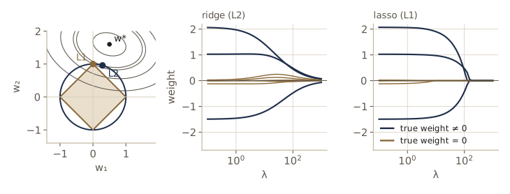
\[\Omega(\mathbf{w}) = \frac{\lambda}{2}\sum_{j=1}^{M} \lvert w_j \rvert^q ,\]with \(q = 2\) giving weight decay. The case \(q = 1\) is the lasso. Its signature is sparsity: with \(\lambda\) large enough, some weights become exactly zero, so the corresponding inputs or basis functions drop out of the model entirely.
Two arguments explain why. The first is geometric. By a Lagrange multiplier argument, minimizing \(E(\mathbf{w}) + \Omega(\mathbf{w})\) is equivalent to minimizing \(E(\mathbf{w})\) subject to \(\sum_j \lvert w_j \rvert^q \le \eta\) for some \(\eta\) that depends on \(\lambda\). The solution is where the smallest error contour touches the constraint region. For \(q = 2\) the region is a ball with a smooth boundary, and the contour generically touches it at a point with no zero coordinate. For \(q = 1\) the region is a diamond whose corners lie on the axes, and the contours usually touch it first at a corner, where some coordinates are zero. For \(q < 1\) the region is not convex and the effect is stronger still.
The second argument is algebraic. When the inputs are orthonormal (\(\mathbf{X}^{\mathrm{T}}\mathbf{X} = \mathbf{I}\)) and \(E = \tfrac12\lVert\mathbf{X}\mathbf{w} - \mathbf{t}\rVert^2\), the problem separates into one scalar problem per weight, \(\tfrac12(w_j - w^{\star}_j)^2 + \tfrac{\lambda}{2}\lvert w_j\rvert^q\), where \(w^{\star}_j\) is the least-squares weight. For \(q = 2\) the minimizer is \(w^{\star}_j/(1 + \lambda)\): every weight shrinks by the same factor, and none reaches zero. For \(q = 1\), the derivative on either side of zero shows the minimizer is the soft-threshold
\[\widehat{w}_j = \operatorname{sign}(w^{\star}_j)\max\left( \lvert w^{\star}_j \rvert - \frac{\lambda}{2},\, 0 \right),\]which sets every weight with \(\lvert w^{\star}_j \rvert \le \lambda/2\) exactly to zero and moves the others toward zero by a constant. For general inputs we minimize the lasso objective by proximal gradient descent (ISTA): take a gradient step on \(E\), then apply the soft-threshold with threshold \(\eta\lambda/2\).
def soft_threshold(v, thr):
    return np.sign(v) * np.maximum(np.abs(v) - thr, 0.0)

def lasso_ista(X, t, lam, steps=3000):
    """Minimize 0.5||X w - t||^2 + (lam/2) sum_j |w_j| by proximal gradient descent."""
    eta = 1.0 / np.linalg.eigvalsh(X.T @ X).max()     # step size 1/L
    w = np.zeros(X.shape[1])
    for _ in range(steps):
        w = soft_threshold(w - eta * X.T @ (X @ w - t), eta * lam / 2)
    return w

def ridge(X, t, lam):
    return np.linalg.solve(X.T @ X + lam * np.eye(X.shape[1]), X.T @ t)

rng_l1 = np.random.default_rng(12)
w_sparse = np.array([2.0, 0.0, 0.0, -1.5, 0.0, 1.0, 0.0, 0.0])   # three nonzero weights
X_s = rng_l1.normal(size=(40, 8))
t_s = X_s @ w_sparse + rng_l1.normal(0, 0.5, 40)
for lam in [1.0, 20.0, 60.0]:
    w_l1, w_l2 = lasso_ista(X_s, t_s, lam), ridge(X_s, t_s, lam)
    print(f"lambda = {lam:4.0f}  L1: {np.round(w_l1, 2)}   exact zeros {np.sum(w_l1 == 0)}")
    print(f"               L2: {np.round(w_l2, 2)}   exact zeros {np.sum(w_l2 == 0)}")
lambda =    1  L1: [ 2.06  0.01 -0.   -1.49 -0.11  1.02 -0.   -0.  ]   exact zeros 3
               L2: [ 1.97  0.06  0.01 -1.46 -0.12  1.03 -0.   -0.  ]   exact zeros 0
lambda =   20  L1: [ 1.73  0.    0.   -1.29 -0.    0.92  0.   -0.  ]   exact zeros 5
               L2: [ 1.12  0.24  0.13 -1.02 -0.09  0.91  0.01 -0.02]   exact zeros 0
lambda =   60  L1: [ 1.06  0.    0.   -0.86 -0.    0.69  0.   -0.  ]   exact zeros 5
               L2: [ 0.63  0.22  0.11 -0.65 -0.05  0.64  0.02 -0.04]   exact zeros 0
At a moderate \(\lambda\) the lasso has found the five irrelevant inputs and set their weights exactly to zero, while ridge regression keeps all eight weights nonzero and merely smaller. The price of the lasso is visible too: it also pulls the surviving weights toward zero by a constant amount. The figure shows the geometry and the full paths.
Regularization lets us train a large model on limited data without severe over-fitting, because it limits the effective complexity. It does not remove the need to choose the complexity; it moves the question from “how many parameters” to “what value of \(\lambda\)”, which is usually answered with a validation set.
Learning curves
So far we have controlled the bias–variance trade-off with the number of parameters, the size of the data set, and \(\lambda\). The training process itself is another control. A learning curve plots a performance measure, such as the training and validation errors, against the iteration number of an iterative method like stochastic gradient descent. Learning curves show how training is going, and they give a practical way to control complexity.
Early stopping
The training error usually falls more or less steadily during training. The error on held-out data, the validation set, typically falls at first and then rises once the network starts fitting noise in the training set. Early stopping keeps the weights from the point of lowest validation error.
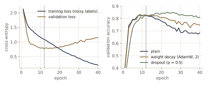
We make over-fitting easy to see by corrupting labels. In the 1000-image MNIST training set we replace 30% of the labels with uniformly random ones (so about 27% end up wrong), keep the validation and test labels clean, and train the multilayer perceptron from before for 40 epochs.
def corrupt_labels(y, frac, seed):
    gen = torch.Generator().manual_seed(seed)
    y = y.clone()
    hit = torch.rand(len(y), generator=gen) < frac
    y[hit] = torch.randint(0, 10, (int(hit.sum()),), generator=gen)
    return y

y_noisy = corrupt_labels(y_tr, 0.3, seed=0)
print(f"fraction of wrong training labels: {(y_noisy != y_tr).float().mean().item():.3f}")

torch.manual_seed(0)
model = mlp()
hist_plain, (stop_epoch, stop_state) = train_mnist(
    model, torch.optim.Adam(model.parameters(), lr=1e-3), X_tr, y_noisy, epochs=40)
for epoch, tr_loss, va_loss, va_acc in hist_plain[::8] + [hist_plain[-1]]:
    print(f"epoch {epoch:2d}  train loss {tr_loss:.3f}  val loss {va_loss:.3f}"
          f"  val acc {va_acc:.3f}")
end_test_acc = evaluate(model, X_te, y_te)[1]
model.load_state_dict(stop_state)
stop_test_acc = evaluate(model, X_te, y_te)[1]
print(f"lowest validation loss at epoch {stop_epoch}")
print(f"test accuracy: early-stopped {stop_test_acc:.3f}   end of training {end_test_acc:.3f}")
fraction of wrong training labels: 0.282
epoch  1  train loss 2.129  val loss 2.085  val acc 0.405
epoch  9  train loss 1.204  val loss 0.815  val acc 0.831
epoch 17  train loss 0.888  val loss 0.798  val acc 0.796
epoch 25  train loss 0.592  val loss 0.893  val acc 0.733
epoch 33  train loss 0.352  val loss 1.017  val acc 0.701
epoch 40  train loss 0.204  val loss 1.143  val acc 0.684
lowest validation loss at epoch 12
test accuracy: early-stopped 0.808   end of training 0.659
The training loss keeps falling as the network memorizes the wrong labels. The validation loss reaches its minimum early and then climbs steeply, and the test accuracy of the early-stopped network is far better than that of the network at the end of training. The test set was not used to choose the stopping point, so its number is a fair estimate.
One common description is that the effective number of parameters starts small and grows during training, so stopping early caps it. For a quadratic error this can be made precise, and the result ties early stopping to weight decay. Start gradient descent at \(\mathbf{w}^{(0)} = \mathbf{0}\) on \(E = E_0 + \tfrac12(\mathbf{w} - \mathbf{w}^{\star})^{\mathrm{T}}\mathbf{H}(\mathbf{w} - \mathbf{w}^{\star})\) with learning rate \(\eta\). The update is \(\mathbf{w}^{(\tau)} - \mathbf{w}^{\star} = (\mathbf{I} - \eta\mathbf{H})(\mathbf{w}^{(\tau-1)} - \mathbf{w}^{\star})\), which separates along the eigenvectors of \(\mathbf{H}\). Unrolling from \(w^{(0)}_j = 0\) gives
\[w^{(\tau)}_j = \left\{ 1 - (1 - \eta\lambda_j)^{\tau} \right\} w^{\star}_j .\]When \(\eta\lambda_j\tau \gg 1\) the factor in braces is close to 1; when \(\eta\lambda_j\tau \ll 1\) it is close to \(\eta\lambda_j\tau\), which is small. Compare the weight-decay factor \(\lambda_j/(\lambda_j + \lambda)\), which is close to 1 for \(\lambda_j \gg \lambda\) and close to \(\lambda_j/\lambda\) for \(\lambda_j \ll \lambda\). The two behave alike if
\[\lambda \approx \frac{1}{\tau\eta},\]so the number of steps times the learning rate plays the role of an inverse regularization coefficient. We check the formula by running gradient descent on a random quadratic with five eigenvalues spread over four decades.
lam_H = np.array([100.0, 10.0, 1.0, 0.1, 0.01])            # eigenvalues of H
Q = np.linalg.qr(rng.normal(size=(5, 5)))[0]                # random eigenvectors
H_q = Q @ np.diag(lam_H) @ Q.T
w_star_q = rng.normal(size=5)
eta_q, tau_q = 0.005, 200                                   # so 1/(tau eta) = 1
w = np.zeros(5)
for _ in range(tau_q):
    w = w - eta_q * H_q @ (w - w_star_q)
print("measured  w_j / w*_j:      ", (Q.T @ w) / (Q.T @ w_star_q))
print("1 - (1 - eta lam_j)^tau:   ", 1 - (1 - eta_q * lam_H) ** tau_q)
print("weight decay, lam = 1/(tau eta):", lam_H / (lam_H + 1 / (tau_q * eta_q)))
measured  w_j / w*_j:       [1.     1.     0.633  0.0952 0.01  ]
1 - (1 - eta lam_j)^tau:    [1.     1.     0.633  0.0952 0.01  ]
weight decay, lam = 1/(tau eta): [0.9901 0.9091 0.5    0.0909 0.0099]
The measured factors match the formula, and they are close to the weight-decay factors: both keep the two stiff directions, both nearly remove the two flat ones, and the middle direction (\(\lambda_j = \lambda\)) is partly kept in both. For a neural network the error is not quadratic and the correspondence is only qualitative, but the lesson carries over: early stopping is a regularizer, and it costs nothing but a validation set.
We can compare it with an explicit regularizer on the same task. We train the same network with AdamW and a decoupled weight decay coefficient of 2, which with learning rate \(\eta = 10^{-3}\) multiplies every weight by \(1 - \eta\lambda = 0.998\) at each step, and look at the test accuracy at the end of training, without early stopping.
torch.manual_seed(0)
model_wd = mlp()
hist_wd, _ = train_mnist(model_wd, torch.optim.AdamW(model_wd.parameters(), lr=1e-3,
                         weight_decay=2.0), X_tr, y_noisy, epochs=40)
print(f"AdamW, weight decay 2: end-of-training test accuracy "
      f"{evaluate(model_wd, X_te, y_te)[1]:.3f}"
      f"   best validation accuracy {max(h[3] for h in hist_wd):.3f}")
AdamW, weight decay 2: end-of-training test accuracy 0.723 best validation accuracy 0.830
Weight decay slows the memorization of the wrong labels and raises the end-of-training accuracy by several points, but on this heavily corrupted data set it falls well short of early stopping. The two combine naturally: it is common to use weight decay and still keep the checkpoint with the best validation error.
Double descent
The classical picture says that test error, plotted against model size, is U-shaped: too small a model underfits, too large a model overfits, and for a given data set very large models should be avoided. Modern deep networks contradict this. They often generalize well with far more parameters than needed to fit the training data perfectly, and they are frequently trained to zero training error without early stopping. The two views are reconciled by double descent: as the model grows, the test error first follows the classical U, peaks around the interpolation threshold (the size at which the model can just fit the training data exactly), and then falls again, often below the classical minimum. The effect has been shown for large networks such as residual networks on image classification (Nakkiran et al., 2019, whose plots Bishop & Bishop §9.3.2 reproduce).
We can see double descent in one of the simplest models there is: least squares on random features. Each feature is a ReLU of a random linear function of the input, \(\phi_j(\mathbf{x}) = \max(0, \mathbf{v}_j^{\mathrm{T}}\mathbf{x} + c_j)\), with \(\mathbf{v}_j\) and \(c_j\) drawn at random and never trained; only the output weights are fitted. With \(P\) features and \(N\) training points, when \(P < N\) we solve ordinary least squares, and when \(P \ge N\) there are infinitely many exact fits and we take the one with the smallest norm, which is what lstsq returns and also what gradient descent from zero converges to. So this is a two-layer network whose first layer is frozen, and \(P\) is its width.
def relu_features(X, V, c):
    return np.maximum(X @ V.T + c, 0.0)

def target_dd(X):
    return np.sin(2 * X.sum(1) / np.sqrt(X.shape[1])) + 0.5 * X[:, 0] * X[:, 1]

rng_dd = np.random.default_rng(13)
N_dd, D_dd = 100, 5
X_dd = rng_dd.normal(size=(N_dd, D_dd))
t_dd = target_dd(X_dd) + rng_dd.normal(0, 0.3, N_dd)
X_dd_test = rng_dd.normal(size=(2000, D_dd))
f_dd_test = target_dd(X_dd_test)                      # noise-free test targets

def random_feature_errors(P, n_draws=8, lam=0.0):
    """Median train and test MSE over draws of the random features.
    lam = 0: least squares (minimum norm when P >= N); lam > 0: ridge via an N x N solve."""
    tr, te = [], []
    for s in range(n_draws):
        g = np.random.default_rng(1000 + s)
        V, c = g.normal(size=(P, D_dd)) / np.sqrt(D_dd), g.normal(size=P)
        Phi_tr, Phi_te = relu_features(X_dd, V, c), relu_features(X_dd_test, V, c)
        if lam == 0.0:
            w = np.linalg.lstsq(Phi_tr, t_dd, rcond=None)[0]
        else:
            w = Phi_tr.T @ np.linalg.solve(Phi_tr @ Phi_tr.T + lam * np.eye(N_dd), t_dd)
        tr.append(np.mean((Phi_tr @ w - t_dd) ** 2))
        te.append(np.mean((Phi_te @ w - f_dd_test) ** 2))
    return np.median(tr), np.median(te)

print("   P   train MSE   test MSE   test MSE (ridge, lambda = 0.1)")
for P in [10, 20, 50, 80, 100, 120, 200, 500, 2000]:
    tr, te = random_feature_errors(P)
    print(f"{P:4d}   {tr:9.4f}   {te:8.3f}   {random_feature_errors(P, lam=0.1)[1]:8.3f}")
   P   train MSE   test MSE   test MSE (ridge, lambda = 0.1)
  10      0.7683      0.773      0.771
  20      0.5431      0.700      0.674
  50      0.1686      0.829      0.589
  80      0.0537      2.459      0.627
 100      0.0034     67.425      0.655
 120      0.0000      3.836      0.498
 200      0.0000      0.709      0.490
 500      0.0000      0.405      0.380
2000      0.0000      0.305      0.303
Read the columns from top to bottom. The training error falls to zero at about \(P = N = 100\), as expected. Among the small models the test error is lowest at about 20 features, the classical sweet spot. It then rises sharply to a peak at \(P = 100\) and falls again; with 2000 features it ends at less than half the classical minimum. With even a little ridge regularization the peak disappears.
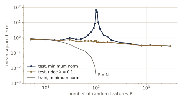
Why the peak? Just at the threshold there is exactly one way to fit all the points, including their noise, and that fit needs enormous weights; the fitted function oscillates wildly between the training points. Past the threshold there are many exact fits, and the minimum-norm rule picks the smoothest of them. As \(P\) grows, the minimum-norm solution becomes smoother still, and the extra capacity is spent on making the fit gentle rather than on fitting noise. The minimum-norm preference is an implicit bias of the solver, and gradient descent from small initial weights has a similar bias; that is part of why stochastic gradient descent on large networks generalizes.
Double descent shows up along other axes too. Plotting test error against the number of training epochs for a large network can show epoch-wise double descent, since training longer increases the effective complexity. Plotting against \(1/\lambda\) for a large model trained to convergence shows the same shape, since small \(\lambda\) means high effective complexity. One consequence is counterintuitive: near the threshold, adding training data moves the threshold to larger models and can make a model of fixed size worse. For Nakkiran et al. (2019), the effective model complexity of a training procedure is the largest number of training points it can still fit with near-zero training error, and the peak appears where this number matches the actual training-set size.
Watch out. Double descent does not mean regularization is obsolete. The peak is largest when the data are noisy and the model is unregularized, and a well-chosen regularizer, as in the ridge column above, removes it. What double descent does show is that parameter count alone is a poor measure of complexity.
Parameter sharing
A penalty such as \(\lVert\mathbf{w}\rVert^2\) reduces complexity by pulling weights toward zero. A harder constraint is to form weights into groups and make every weight in a group equal to one shared value, which is itself learned. This is weight sharing (also parameter sharing or parameter tying). The number of degrees of freedom is then smaller than the number of connections, and the pattern of sharing usually encodes an invariance known in advance. Convolutional networks are the main example: one filter is shared across all image positions, which gives the equivariance of the previous section.
The gradient with respect to a shared parameter is the sum of the gradients with respect to each of its uses, since by the chain rule every use contributes a term. Automatic differentiation handles this for free whenever the same tensor appears in several places.
torch.manual_seed(3)
shared = nn.Linear(4, 4)                         # used twice: a tied two-layer map
x = torch.randn(6, 4)
loss = shared(torch.tanh(shared(x))).pow(2).sum()
loss.backward()
g_tied = shared.weight.grad.clone()

# the same computation with two untied copies holding identical values
first, second = copy.deepcopy(shared), copy.deepcopy(shared)
second(torch.tanh(first(x))).pow(2).sum().backward()
print(f"tied gradient equals the sum of the untied gradients: "
      f"{torch.allclose(g_tied, first.weight.grad + second.weight.grad)}")
tied gradient equals the sum of the untied gradients: True
Hard sharing only applies when we know in advance which weights should be equal.
Soft weight sharing
Soft weight sharing (Nowlan and Hinton, 1992) relaxes the constraint: a penalty encourages weights to form groups of similar values, and the learning algorithm decides the groups, their centers, and their spreads. Weight decay can be read as a single Gaussian prior centered at zero, which pulls all weights toward one value. Replacing it by a mixture of Gaussians lets weights gather around several values:
\[p(\mathbf{w}) = \prod_i \sum_{j=1}^{K} \pi_j \, \mathcal{N}(w_i \mid \mu_j, \sigma_j^2),\]where the means \(\mu_j\), variances \(\sigma_j^2\), and mixing coefficients \(\pi_j\) are learned along with the weights (mixtures of Gaussians are the subject of Intro to ML, module 09). The negative logarithm gives the regularizer
\[\Omega(\mathbf{w}) = -\sum_i \ln\left( \sum_{j=1}^{K} \pi_j \, \mathcal{N}(w_i \mid \mu_j, \sigma_j^2) \right),\]and we minimize \(\widetilde{E}(\mathbf{w}) = E(\mathbf{w}) + \lambda\Omega(\mathbf{w})\) jointly over the weights and the mixture parameters by gradient descent. The derivatives are easiest to read with the responsibilities
\[\gamma_j(w_i) = \frac{\pi_j \, \mathcal{N}(w_i \mid \mu_j, \sigma_j^2)}{\sum_k \pi_k \, \mathcal{N}(w_i \mid \mu_k, \sigma_k^2)},\]the posterior probability that component \(j\) generated weight \(w_i\). Differentiating \(-\ln \sum_j \pi_j \mathcal{N}(w_i \mid \mu_j, \sigma_j^2)\) with respect to \(w_i\) brings down, for each component, its share \(\gamma_j(w_i)\) times the derivative of \(-\ln\mathcal{N}\), which is \((w_i - \mu_j)/\sigma_j^2\). So
\[\frac{\partial \widetilde{E}}{\partial w_i} = \frac{\partial E}{\partial w_i} + \lambda\sum_j \gamma_j(w_i)\,\frac{w_i - \mu_j}{\sigma_j^2}.\]Each weight is pulled toward the centers of the components, with a force weighted by how responsible each component is for it. To keep variances positive and mixing coefficients on the simplex we optimize unconstrained variables, \(\sigma_j^2 = \exp(\xi_j)\) and \(\pi_j = \exp(\eta_j)/\sum_k \exp(\eta_k)\) (a softmax). The same kind of calculation gives
\[\frac{\partial \widetilde{E}}{\partial \mu_j} = \lambda\sum_i \gamma_j(w_i)\,\frac{\mu_j - w_i}{\sigma_j^2}, \qquad \frac{\partial \widetilde{E}}{\partial \xi_j} = \frac{\lambda}{2}\sum_i \gamma_j(w_i)\left( 1 - \frac{(w_i - \mu_j)^2}{\sigma_j^2} \right), \qquad \frac{\partial \widetilde{E}}{\partial \eta_j} = \lambda\sum_i \left\{ \pi_j - \gamma_j(w_i) \right\}.\]Each has a clear reading: a center moves toward the responsibility-weighted mean of its weights, a variance toward their responsibility-weighted spread, and a mixing coefficient toward the average responsibility. We implement \(\Omega\) with a log-sum-exp and check all four formulas against autograd.
class MixturePrior(nn.Module):
    """Omega(w) = -sum_i ln sum_j pi_j N(w_i | mu_j, sigma_j^2), with pi = softmax(eta)
    and sigma^2 = exp(xi)."""
    def __init__(self, K, mu_range=1.0, log_var=-1.0):
        super().__init__()
        self.eta = nn.Parameter(torch.zeros(K))
        self.mu = nn.Parameter(torch.linspace(-mu_range, mu_range, K))
        self.xi = nn.Parameter(torch.full((K,), log_var))

    def log_joint(self, w):                        # ln pi_j + ln N(w_i | mu_j, sigma_j^2)
        var = torch.exp(self.xi)
        return (torch.log_softmax(self.eta, 0) - 0.5 * torch.log(2 * torch.pi * var)
                - 0.5 * (w[:, None] - self.mu) ** 2 / var)

    def forward(self, w):
        return -torch.logsumexp(self.log_joint(w), dim=1).sum()

torch.manual_seed(4)
prior = MixturePrior(3)
w = torch.randn(20, requires_grad=True)
prior(w).backward()                                # lambda = 1, E = 0 for the check
with torch.no_grad():
    gamma = torch.softmax(prior.log_joint(w), dim=1)          # responsibilities (20, 3)
    var, pi = torch.exp(prior.xi), torch.softmax(prior.eta, 0)
    diff = w[:, None] - prior.mu
    formulas = {"w": (gamma * diff / var).sum(1), "mu": (-gamma * diff / var).sum(0),
                "xi": 0.5 * (gamma * (1 - diff ** 2 / var)).sum(0), "eta": (pi - gamma).sum(0)}
autograd = {"w": w.grad, "mu": prior.mu.grad, "xi": prior.xi.grad, "eta": prior.eta.grad}
for k in formulas:
    match = torch.allclose(formulas[k], autograd[k], atol=1e-6)
    print(f"dOmega/d{k:3s} formula matches autograd: {match}")
dOmega/dw   formula matches autograd: True
dOmega/dmu  formula matches autograd: True
dOmega/dxi  formula matches autograd: True
dOmega/deta formula matches autograd: True
A small experiment shows the prior at work. We fit a linear model with 40 weights whose true values are drawn from \(\{-1.5, 0, 1.5\}\), from only 50 noisy examples, first by least squares, then with weight decay, then with a three-component soft-sharing prior.
g_sw = torch.Generator().manual_seed(5)
D_sw, N_sw = 40, 50
w_true = torch.tensor([-1.5, 0.0, 1.5])[torch.randint(0, 3, (D_sw,), generator=g_sw)]
X_sw = torch.randn(N_sw, D_sw, generator=g_sw)
t_sw = X_sw @ w_true + 0.8 * torch.randn(N_sw, generator=g_sw)

def fit_linear(lam, soft, steps=1500):
    torch.manual_seed(0)
    w = nn.Parameter(torch.zeros(D_sw))
    prior = MixturePrior(3)
    params = [w] + (list(prior.parameters()) if soft else [])
    opt = torch.optim.Adam(params, lr=0.02)
    for _ in range(steps):
        E = 0.5 * ((X_sw @ w - t_sw) ** 2).sum()
        reg = lam * prior(w) if soft else 0.5 * lam * (w ** 2).sum()
        opt.zero_grad()
        (E + reg).backward()
        opt.step()
    return w.detach(), prior

w_ls = torch.linalg.lstsq(X_sw, t_sw.unsqueeze(1)).solution.squeeze()
w_l2, _ = fit_linear(1.0, soft=False)
w_soft, prior = fit_linear(1.0, soft=True)
for name, w in [("least squares", w_ls), ("weight decay ", w_l2), ("soft sharing ", w_soft)]:
    print(f"{name}  ||w - w_true||^2 = {((w - w_true) ** 2).sum().item():.3f}")
order = torch.argsort(prior.mu.detach())
print("learned centers:", prior.mu.detach()[order].numpy().round(3),
      "  mixing:", torch.softmax(prior.eta.detach(), 0)[order].numpy().round(2),
      "  std devs:", torch.exp(0.5 * prior.xi.detach())[order].numpy().round(3))
least squares  ||w - w_true||^2 = 1.304
weight decay   ||w - w_true||^2 = 1.730
soft sharing   ||w - w_true||^2 = 0.015
learned centers: [-1.482  0.027  1.516]   mixing: [0.42 0.28 0.3 ]   std devs: [0.003 0.002 0.003]
With 50 equations for 40 unknowns, least squares is noisy, and weight decay, which pulls every weight toward zero, makes things slightly worse because two thirds of the true weights are far from zero. The mixture prior discovers the three values, puts its centers close to \(-1.5\), \(0\), and \(1.5\), and snaps the weights onto them, which cuts the error by a large factor.
Watch out. The learned standard deviations have collapsed to almost zero. This is the same singularity that affects maximum likelihood for Gaussian mixtures: a component that sits exactly on some weights can shrink its variance without limit and make \(\Omega\) arbitrarily negative. It happened to be harmless here because the true weights really are clustered, but in general one bounds the variances from below or puts a prior on them.
Soft tying of parameters has other uses. One of them links a generative model and a discriminative model of the same data by a soft penalty on the difference of their parameters. The generative model can learn from unlabeled data, the discriminative one copes better when the model is misspecified, and the tie gives a principled hybrid of the two, useful when labeled data are scarce (Bishop & Bishop §9.4.1 gives the reference).
Residual connections
Depth is a large part of what makes deep networks powerful, and deeper networks often generalize better. But deep networks are harder to train. Module 07 showed how careful initialization and batch normalization tame vanishing and exploding gradients; even with both, very deep plain networks remain difficult. Residual connections are the architectural change that made networks with hundreds of layers routine, and they count as regularization in the broad sense of this module: they shape which functions are easy to reach.
Why deep plain stacks train badly
We build one class that can be either a plain deep network or a residual one with exactly the same parameters. A plain layer computes \(\mathbf{z}_l = \mathbf{W}_l\,\mathrm{ReLU}(\mathbf{z}_{l-1}) + \mathbf{b}_l\); a residual block adds its input back:
\[\mathbf{z}_l = \mathbf{z}_{l-1} + \mathbf{F}_l(\mathbf{z}_{l-1}), \qquad \mathbf{F}_l(\mathbf{z}) = \mathbf{W}_l\,\mathrm{ReLU}(\mathbf{z}) + \mathbf{b}_l .\]The task is two interleaved spirals in the plane, and the networks have 30 hidden layers of width 32.
class DeepMLP(nn.Module):
    """Input layer, `depth` hidden layers of width H, output layer.
    plain:    z_l = W_l ReLU(z_{l-1}) + b_l
    residual: z_l = z_{l-1} + W_l ReLU(z_{l-1}) + b_l"""
    def __init__(self, D, H, K, depth, residual, he_init=False):
        super().__init__()
        self.inp = nn.Linear(D, H)
        self.layers = nn.ModuleList([nn.Linear(H, H) for _ in range(depth)])
        self.out = nn.Linear(H, K)
        self.residual = residual
        if he_init:                                 # module 07: variance 2 / fan_in
            for layer in self.layers:
                nn.init.kaiming_normal_(layer.weight, nonlinearity="relu")
                nn.init.zeros_(layer.bias)

    def forward(self, x, drop_layer=None):
        z = self.inp(x)
        for l, layer in enumerate(self.layers):
            if l == drop_layer:                     # used later to delete one layer
                continue
            f = layer(F.relu(z))
            z = z + f if self.residual else f
        return self.out(F.relu(z))

def spirals(n, gen):
    k = torch.randint(0, 2, (n,), generator=gen)
    r = torch.rand(n, generator=gen)
    angle = 3 * torch.pi * r + torch.pi * k
    X = torch.stack([r * torch.cos(angle), r * torch.sin(angle)], 1)
    return 2 * X + 0.06 * torch.randn(n, 2, generator=gen), k

g_sp = torch.Generator().manual_seed(3)
X_sp, t_sp = spirals(300, g_sp)
X_sp_val, t_sp_val = spirals(1000, g_sp)

configs = [("plain, default init", False, False), ("plain, He init     ", False, True),
           ("residual           ", True, False)]
for name, residual, he in configs:
    torch.manual_seed(1)
    net = DeepMLP(2, 32, 2, depth=30, residual=residual, he_init=he)
    F.cross_entropy(net(X_sp), t_sp).backward()
    norms = [layer.weight.grad.norm().item() for layer in net.layers]
    print(f"{name}  gradient norm, layer 1: {norms[0]:.1e}   layer 15: {norms[14]:.1e}"
          f"   layer 30: {norms[29]:.1e}")
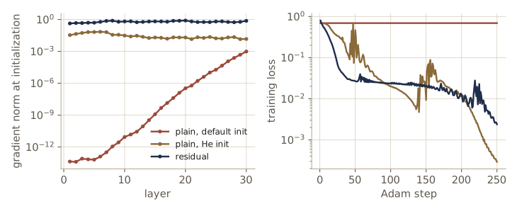
plain, default init  gradient norm, layer 1: 4.3e-14   layer 15: 1.2e-09   layer 30: 9.7e-04
plain, He init       gradient norm, layer 1: 3.4e-02   layer 15: 2.0e-02   layer 30: 1.5e-02
residual             gradient norm, layer 1: 4.2e-01   layer 15: 6.6e-01   layer 30: 7.5e-01
With PyTorch’s default initialization, each plain layer shrinks the signal, and between the last layer and the first the gradient norm falls by about ten orders of magnitude: the early layers will never move. He initialization, from module 07, keeps the gradient norms roughly level at the start. The residual network has level gradients even with the default initialization, because the identity path carries the gradient backward unchanged: differentiating \(\mathbf{z}_l = \mathbf{z}_{l-1} + \mathbf{F}_l(\mathbf{z}_{l-1})\) gives
\[\frac{\partial \mathbf{z}_l}{\partial \mathbf{z}_{l-1}} = \mathbf{I} + \frac{\partial \mathbf{F}_l}{\partial \mathbf{z}_{l-1}},\]so the product of these Jacobians through the network always contains the identity term, and never collapses to zero just because the individual \(\partial\mathbf{F}_l/\partial\mathbf{z}_{l-1}\) are small. Now we train all three with Adam.
def train_spirals(net, steps=250, lr=1e-3):
    opt = torch.optim.Adam(net.parameters(), lr=lr)
    losses = []
    for step in range(steps):
        loss = F.cross_entropy(net(X_sp), t_sp)
        opt.zero_grad()
        loss.backward()
        opt.step()
        losses.append(loss.item())
    return losses

def spiral_accuracy(net, **kw):
    with torch.no_grad():
        return (net(X_sp_val, **kw).argmax(1) == t_sp_val).float().mean().item()

deep_nets = {}
for name, residual, he in configs:
    torch.manual_seed(1)
    net = DeepMLP(2, 32, 2, depth=30, residual=residual, he_init=he)
    losses = train_spirals(net)
    deep_nets[name.strip()] = net
    print(f"{name}  loss at steps 1, 50, 250: {losses[0]:.3f} {losses[49]:.3f}"
          f" {losses[-1]:.3f}   validation accuracy {spiral_accuracy(net):.3f}")
plain, default init  loss at steps 1, 50, 250: 0.690 0.690 0.690   validation accuracy 0.524
plain, He init       loss at steps 1, 50, 250: 0.692 0.466 0.000   validation accuracy 0.972
residual             loss at steps 1, 50, 250: 0.798 0.027 0.002   validation accuracy 0.976
The plain network with default initialization never leaves the chance-level loss of \(\ln 2 \approx 0.693\). With He initialization the plain network does train on this small problem. The residual network, with no special initialization, gets there much faster (a loss of 0.027 after 50 steps, against 0.466), and both end with about 97% validation accuracy. That He-initialized plain networks can train at this depth is a real success of module 07’s analysis; the harder difficulties appear with depth and with the kind of optimization used for large models, and they are subtler than vanishing gradients.
One such difficulty is called shattered gradients (Balduzzi et al., 2017). A deep ReLU network divides its input space into a number of linear pieces that grows exponentially with depth, so the gradient of its output with respect to its input, and hence the gradient of the error with respect to early weights, jumps around more and more as depth increases. Gradient-based optimization assumes that the gradient at nearby points is similar; when it is not, steps in early layers are close to random. We can measure this directly: take networks with one input and one output, compute \(\partial y / \partial x\) on a fine grid of inputs, and measure the correlation between the derivatives at neighboring grid points.
x_grid = torch.linspace(-3, 3, 600).unsqueeze(1).requires_grad_(True)

def neighbor_correlation(net):
    dy_dx, = torch.autograd.grad(net(x_grid).sum(), x_grid)
    g = dy_dx.squeeze().numpy()
    return np.corrcoef(g[:-1], g[1:])[0, 1]

for name, depth, residual, he in [("2 layers, plain     ", 1, False, True),
                                  ("50 layers, plain    ", 50, False, True),
                                  ("50 layers, residual ", 50, True, False)]:
    corr = []
    for seed in range(5):
        torch.manual_seed(seed)
        corr.append(neighbor_correlation(DeepMLP(1, 64, 1, depth, residual, he_init=he)))
    print(f"{name} correlation of dy/dx at neighboring inputs: {np.mean(corr):.3f}")
2 layers, plain      correlation of dy/dx at neighboring inputs: 0.985
50 layers, plain     correlation of dy/dx at neighboring inputs: 0.773
50 layers, residual  correlation of dy/dx at neighboring inputs: 0.980
The shallow network’s derivative is almost perfectly correlated from one grid point to the next. The 50-layer plain network (with a good initialization) has a noticeably shattered derivative, and the 50-layer residual network is as smooth as the shallow one. Visualizations of the error surface tell the same story: adding residual connections to a very deep network turns a rugged loss landscape into a much smoother one (Li et al., 2017, arXiv:1712.09913).
Residual blocks
A residual block is any function \(\mathbf{F}_l\) wrapped with a skip connection, \(\mathbf{z}_l = \mathbf{F}_l(\mathbf{z}_{l-1}) + \mathbf{z}_{l-1}\), and a residual network (ResNet; He et al., 2015) is a sequence of such blocks. The name comes from rearranging: \(\mathbf{F}_l(\mathbf{z}_{l-1}) = \mathbf{z}_l - \mathbf{z}_{l-1}\), so each block learns only the change, the residual, relative to the identity. If a block is not needed, its parameters only have to become small for the block to pass its input through, which is much easier than learning an identity map through a nonlinearity.
The block function can be a single layer, as above, or several linear, nonlinear, and normalization layers. With alternating linear layers and ReLUs there are two natural places for the skip. If each block ends with a ReLU, the branch can only ever add nonnegative values. Putting the ReLU first, so that a block computes \(\mathbf{z} + \mathbf{W}\,\mathrm{ReLU}(\mathbf{z})\) as in our DeepMLP, lets the branch add values of either sign, and this pre-activation ordering is the more common choice. Residual networks usually include batch normalization in each branch as well.
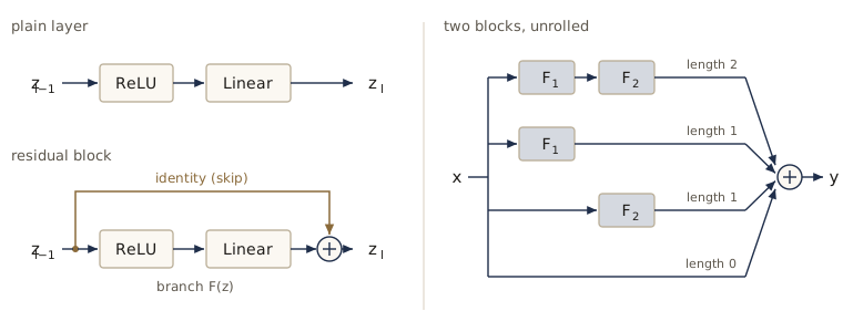
The addition requires \(\mathbf{z}_{l-1}\) and \(\mathbf{F}_l(\mathbf{z}_{l-1})\) to have the same dimension. Where a network changes width, the skip gets a learnable matrix of its own, \(\mathbf{z}_l = \mathbf{F}_l(\mathbf{z}_{l-1}) + \mathbf{W}\mathbf{z}_{l-1}\) with \(\mathbf{W}\) not square.
Residual networks as ensembles and as differential equations
Write out three blocks, \(\mathbf{z}_1 = \mathbf{F}_1(\mathbf{x}) + \mathbf{x}\), \(\mathbf{z}_2 = \mathbf{F}_2(\mathbf{z}_1) + \mathbf{z}_1\), \(\mathbf{y} = \mathbf{F}_3(\mathbf{z}_2) + \mathbf{z}_2\), and substitute:
\[\mathbf{y} = \mathbf{F}_3\big(\mathbf{F}_2(\mathbf{F}_1(\mathbf{x}) + \mathbf{x}) + \mathbf{F}_1(\mathbf{x}) + \mathbf{x}\big) + \mathbf{F}_2(\mathbf{F}_1(\mathbf{x}) + \mathbf{x}) + \mathbf{F}_1(\mathbf{x}) + \mathbf{x}.\]The output is a sum of terms computed by sub-networks of different depths. If the blocks were linear, the expansion would be exact as a sum over all \(2^L\) subsets of blocks, with \(\binom{L}{k}\) paths of length \(k\); with nonlinear blocks the paths are entangled but the picture is still useful. A residual network contains the full deep network as one of its paths, so it loses no representational power, while most of its paths are of moderate length, which keeps the error surface closer to that of a shallow network.
The ensemble view makes a prediction we can test. Deleting one layer from a plain network breaks the single chain of computation. Deleting one block from a residual network only removes the paths through that block, and the many remaining paths should still give a sensible output.
for name in ["plain, He init", "residual"]:
    net = deep_nets[name]
    accs = [spiral_accuracy(net, drop_layer=l) for l in range(30)]
    print(f"{name:15s} intact {spiral_accuracy(net):.3f}   one layer deleted: "
          f"mean {np.mean(accs):.3f}, worst {np.min(accs):.3f}")
plain, He init  intact 0.972   one layer deleted: mean 0.532, worst 0.030
residual        intact 0.976   one layer deleted: mean 0.839, worst 0.656
The residual network keeps most of its accuracy when any one of its 30 blocks is deleted (0.84 on average, 0.66 in the worst case), while deleting a single layer from the plain network typically brings it down to chance, and in the worst case below it. The residual network behaves like a collection of many shallower networks rather than one very deep chain.
There is a second reading. If we scale each block, \(\mathbf{z}_l = \mathbf{z}_{l-1} + h\,\mathbf{f}(\mathbf{z}_{l-1}, l)\), the update is one step of Euler’s method for the ordinary differential equation \(d\mathbf{z}/dt = \mathbf{f}(\mathbf{z}, t)\) with step size \(h\). A deep residual network is then a discretized continuous-time flow, and taking the limit of infinitely many infinitesimal blocks gives neural ordinary differential equations, which return in module 18 as a way to build invertible generative models.
Model averaging
If we have trained several models for the same problem, then instead of picking the best one we can often do better by averaging their predictions. A set of models combined this way is a committee or ensemble. For models with probabilistic outputs the combined predictive distribution is the average
\[p(\mathbf{y} \mid \mathbf{x}) = \frac{1}{L}\sum_{l=1}^{L} p_l(\mathbf{y} \mid \mathbf{x}),\]where \(p_l\) is the prediction of model \(l\).
Why averaging helps
Take a regression problem with true function \(h(\mathbf{x})\) and \(M\) trained models \(y_m(\mathbf{x}) = h(\mathbf{x}) + \epsilon_m(\mathbf{x})\), where \(\epsilon_m\) is the error of model \(m\). The average squared error of the individual models is
\[E_{\mathrm{AV}} = \frac{1}{M}\sum_{m=1}^{M} \mathbb{E}_{\mathbf{x}}\left[ \epsilon_m(\mathbf{x})^2 \right],\]and the committee \(y_{\mathrm{COM}} = \frac{1}{M}\sum_m y_m\) has error
\[E_{\mathrm{COM}} = \mathbb{E}_{\mathbf{x}}\left[ \left( \frac{1}{M}\sum_{m=1}^{M} \epsilon_m(\mathbf{x}) \right)^2 \right] = \frac{1}{M^2}\sum_{m=1}^{M}\sum_{l=1}^{M} \mathbb{E}_{\mathbf{x}}\left[ \epsilon_m(\mathbf{x})\,\epsilon_l(\mathbf{x}) \right].\]If the errors are uncorrelated, \(\mathbb{E}_{\mathbf{x}}[\epsilon_m\epsilon_l] = 0\) for \(m \neq l\), only the \(M\) diagonal terms survive and
\[E_{\mathrm{COM}} = \frac{1}{M}E_{\mathrm{AV}} .\]Averaging \(M\) models would divide the error by \(M\). That is much too optimistic in practice, because models trained on the same data tend to make the same mistakes, so their errors are strongly correlated. What does always hold is weaker: since the square is convex, Jensen’s inequality gives \(\left( \frac1M\sum_m\epsilon_m \right)^2 \le \frac1M\sum_m\epsilon_m^2\) at every \(\mathbf{x}\), hence
\[E_{\mathrm{COM}} \le E_{\mathrm{AV}} .\]A committee is never worse than its average member. In the language of the bias–variance decomposition, averaging reduces the variance term and leaves the bias alone (Intro to ML, module 14 has the full treatment of committees).
The gain depends on making the members differ. With only one data set, two common sources of diversity are different random initializations (and mini-batch orders) and different training sets drawn by the bootstrap: draw \(N\) points from the \(N\) training points with replacement, so that some points appear several times and others not at all, and repeat to get \(L\) data sets of size \(N\). Training one model per bootstrap set and averaging is bagging, for bootstrap aggregation (Breiman, 1996). Members can also differ in architecture.
We compare the two on a one-dimensional regression problem with a gap in the training inputs. Rather than looping over ten networks, we train all members at once: each weight tensor gets a leading “member” dimension, and torch.baddbmm evaluates all members in one batched matrix product. The members still share nothing but the data they are given.
def h_true(x):
    return torch.sin(3 * x) + 0.3 * x

g_1d = torch.Generator().manual_seed(4)
N_1d = 24
X_1d = torch.cat([torch.rand(N_1d // 2, 1, generator=g_1d) * 1.2 - 1.5,     # [-1.5, -0.3]
                  torch.rand(N_1d // 2, 1, generator=g_1d) * 1.2 + 0.3])    # [0.3, 1.5]
T_1d = h_true(X_1d) + 0.2 * torch.randn(N_1d, 1, generator=g_1d)
x_plot = torch.linspace(-2, 2, 401).unsqueeze(1)
in_data = (((x_plot > -1.5) & (x_plot < -0.3)) | ((x_plot > 0.3) & (x_plot < 1.5))).squeeze()

class Committee(nn.Module):
    """M independent 1-H-H-1 tanh networks evaluated together with batched matrix products."""
    def __init__(self, M, H=64):
        super().__init__()
        def layer(n_in, n_out):
            bound = 1 / np.sqrt(n_in)
            W = nn.Parameter(torch.empty(M, n_in, n_out).uniform_(-bound, bound))
            b = nn.Parameter(torch.empty(M, 1, n_out).uniform_(-bound, bound))
            return W, b
        (self.W1, self.b1), (self.W2, self.b2), (self.W3, self.b3) = \
            layer(1, H), layer(H, H), layer(H, 1)

    def forward(self, X):                          # X: (N, 1) shared, or (M, N, 1) per member
        if X.dim() == 2:
            X = X.expand(self.W1.shape[0], *X.shape)
        z = torch.tanh(torch.baddbmm(self.b1, X, self.W1))
        z = torch.tanh(torch.baddbmm(self.b2, z, self.W2))
        return torch.baddbmm(self.b3, z, self.W3)  # (M, N, 1)

def fit_committee(com, X, T, steps=1000, lr=0.01):
    opt = torch.optim.Adam(com.parameters(), lr=lr)
    for _ in range(steps):
        loss = ((com(X) - T) ** 2).mean(dim=(1, 2)).sum()   # sum of the members' losses
        opt.zero_grad()
        loss.backward()
        opt.step()
    return com

def committee_report(name, com):
    with torch.no_grad():
        P = com(x_plot)[:, in_data]                          # predictions where there is data
    err = P - h_true(x_plot[in_data])
    e_av = (err ** 2).mean().item()
    e_com = (err.mean(0) ** 2).mean().item()
    E = err.squeeze(-1)
    C = (E @ E.T) / E.shape[1]                               # E_x[eps_m eps_l]
    corr = C / torch.sqrt(torch.outer(C.diag(), C.diag()))
    rho = corr.fill_diagonal_(0).sum() / (M_com * (M_com - 1))  # mean off-diagonal
    print(f"{name}  E_AV {e_av:.4f}   E_COM {e_com:.4f}   E_AV/M {e_av / M_com:.4f}"
          f"   mean error correlation {rho.item():.2f}")

M_com = 10
torch.manual_seed(0)
seeds_only = fit_committee(Committee(M_com), X_1d, T_1d)
boot_idx = torch.randint(0, N_1d, (M_com, N_1d), generator=torch.Generator().manual_seed(1))
torch.manual_seed(0)
bagged = fit_committee(Committee(M_com), X_1d[boot_idx], T_1d[boot_idx])
committee_report("different seeds", seeds_only)
committee_report("bagging        ", bagged)
different seeds  E_AV 0.0563   E_COM 0.0531   E_AV/M 0.0056   mean error correlation 0.95
bagging          E_AV 0.0834   E_COM 0.0325   E_AV/M 0.0083   mean error correlation 0.38
The members that differ only in their initialization have errors that are almost perfectly correlated, so their committee is barely better than a single member. The bagged members are individually worse, since each sees only about 63% of the distinct points, but their errors are much less correlated, and the committee beats both the seed-only committee and its own members by a wide margin. Neither reaches the \(E_{\mathrm{AV}}/M\) of the uncorrelated ideal.
Boosting (Freund and Schapire, 1996) is a different way to combine models. Base classifiers are trained in sequence, each on a weighted version of the data in which the points misclassified by the previous classifiers get larger weights, and the final prediction is a weighted vote. Boosting can turn base classifiers that are only slightly better than chance into a strong classifier; Intro to ML, module 14 derives AdaBoost. The main drawback of every committee method is cost: training and prediction are multiplied by the number of members, which for large networks is often too much.
Dropout
Dropout (Srivastava et al., 2014) gets much of the benefit of an ensemble from a single network. During training, each time an example is presented, every non-output unit is deleted at random, together with its connections, and the forward and backward passes run on the thinned network. Every presentation of an example draws a fresh set of deletions. Deleting a unit is the same as setting its output to zero, so dropout multiplies the activation \(z_{ni}\) of unit \(i\) on example \(n\) by a mask \(R_{ni} \in \{0, 1\}\) with \(p(R_{ni} = 1) = \rho\). Values around \(\rho = 0.5\) for hidden units and \(\rho = 0.8\) for inputs are common starting points. With mini-batches the gradient is averaged over the thinned networks of the batch, as usual.
A network with \(M\) droppable units has \(2^M\) thinned versions, so dropout trains an astronomically large ensemble. Unlike a real ensemble, its members are never trained to convergence individually (most are never sampled at all) and they are not independent: they share weights with the full network and with one another. The gradients are noisy, so training with dropout takes longer, and the training loss fluctuates more, which makes it harder to judge from the loss alone whether optimization is working.
At test time the ensemble prediction would be
\[p(\mathbf{y} \mid \mathbf{x}) = \sum_{\mathbf{R}} p(\mathbf{R})\, p(\mathbf{y} \mid \mathbf{x}, \mathbf{R}),\]a sum over all masks. Two approximations are used. Monte Carlo dropout keeps dropout on at test time and averages the predictions of a modest number of sampled masks, such as 10 to 50. Weight scaling runs the full network once, with the activations rescaled so that each unit receives on average the same input as during training. If unit \(i\) is present with probability \(\rho\), its expected contribution during training was \(\rho\) times its full value, so at test time we multiply its outgoing weights by \(\rho\). Modern libraries use the equivalent inverted dropout: divide the kept activations by \(\rho\) during training, so that \(\mathbb{E}[R_{ni}z_{ni}/\rho] = z_{ni}\), and use the network unchanged at test time.
Watch out. PyTorch’s
nn.Dropout(p)takes the probability of dropping a unit, \(p = 1 - \rho\), not the probability of keeping it.nn.Dropout(0.2)keeps 80% of the units. It is active only inmodel.train()mode and does nothing aftermodel.eval(), so forgetting to switch modes silently changes the predictions.
Here is inverted dropout written with tensor operations, checked against nn.Dropout with the same random seed.
class InvertedDropout(nn.Module):
    """Keep each unit with probability rho = 1 - p and scale kept units by 1/rho during
    training; identity in eval mode."""
    def __init__(self, p):
        super().__init__()
        self.rho = 1.0 - p

    def forward(self, z):
        if not self.training:
            return z
        R = torch.empty_like(z).bernoulli_(self.rho)   # mask R_ni ~ Bernoulli(rho)
        return z * R.div_(self.rho)                    # inverted scaling 1/rho

z = torch.randn(4, 1000)
ours, theirs = InvertedDropout(0.3), nn.Dropout(0.3)
torch.manual_seed(7)
a = ours(z)
torch.manual_seed(7)
b = theirs(z)
print(f"training mode: identical to nn.Dropout: {torch.equal(a, b)}"
      f"   fraction zeroed {(a == 0).float().mean().item():.3f}")
ours.eval(); theirs.eval()
unchanged = torch.equal(ours(z), z) and torch.equal(theirs(z), z)
print(f"eval mode: both return the input unchanged: {unchanged}")
ours.train()
mean_out = torch.stack([ours(z) for _ in range(2000)]).mean(0)
print(f"average over 2000 masks vs input: mean absolute difference "
      f"{(mean_out - z).abs().mean().item():.4f}")
training mode: identical to nn.Dropout: True   fraction zeroed 0.294
eval mode: both return the input unchanged: True
average over 2000 masks vs input: mean absolute difference 0.0092
The mask and scaling match PyTorch exactly, eval mode is the identity, and averaging over many masks recovers the input up to Monte Carlo error, which is the property that justifies weight scaling for a single layer. For a whole nonlinear network weight scaling is only an approximation to the ensemble average.
Why does dropout help? One view is the ensemble one above. A Bayesian view: a fully Bayesian prediction would average all \(2^M\) thinned networks weighted by their posterior probabilities, which is far too expensive; dropout averages them with equal weights. A third view is about co-adaptation: in an ordinary network, units can become tuned to cancel each other’s errors on particular training points, which does not generalize. With dropout, no unit can count on any other being present, so each must be useful on its own in many contexts.
For a linear model the regularization can be computed exactly. Take \(y_n = \sum_i w_i R_{ni}x_{ni}/\rho\) with inverted dropout on the inputs and a sum-of-squares error. Using \(\mathbb{E}[R_{ni}] = \rho\) and \(\mathbb{E}[R_{ni}R_{nj}] = \rho^2\) for \(i \ne j\) and \(\rho\) for \(i = j\), the variance of \(y_n\) is \(\sum_i w_i^2x_{ni}^2(1-\rho)/\rho\), so
\[\mathbb{E}_{\mathbf{R}}\left[ \sum_n (t_n - y_n)^2 \right] = \sum_n \left( t_n - \mathbf{w}^{\mathrm{T}}\mathbf{x}_n \right)^2 + \frac{1-\rho}{\rho}\sum_i \left( \sum_n x_{ni}^2 \right) w_i^2 .\]Dropout on the inputs of a linear model is a quadratic penalty whose coefficient for each weight grows with the energy of its input. A Monte Carlo check:
rho_lin = 0.7
X_d, t_d, w_d = rng.normal(size=(30, 4)), rng.normal(size=30), rng.normal(size=4)
R_d = rng.random((20000, 30, 4)) < rho_lin                  # 20000 sampled masks
mc = np.mean(np.sum((t_d - (R_d * X_d) @ w_d / rho_lin) ** 2, axis=1))
exact = (np.sum((t_d - X_d @ w_d) ** 2)
         + (1 - rho_lin) / rho_lin * np.sum((X_d ** 2).sum(0) * w_d ** 2))
print(f"Monte Carlo average error {mc:.3f}   formula {exact:.3f}")
Monte Carlo average error 107.461 formula 107.267
Now dropout on the corrupted-label MNIST task. We use \(\rho = 0.5\) on both hidden layers (p_drop=0.5) and train for 40 epochs, then compare weight scaling (eval mode) with Monte Carlo dropout over 20 masks.
torch.manual_seed(0)
model_do = mlp(p_drop=0.5)
hist_do, _ = train_mnist(model_do, torch.optim.Adam(model_do.parameters(), lr=1e-3),
                         X_tr, y_noisy, epochs=40)
_, acc_scaled = evaluate(model_do, X_te, y_te)             # eval mode = weight scaling
model_do.train()                                           # masks on for Monte Carlo
torch.manual_seed(1)
with torch.no_grad():
    probs = torch.stack([F.softmax(model_do(X_te), 1) for _ in range(20)]).mean(0)
acc_mc = (probs.argmax(1) == y_te).float().mean().item()
print(f"dropout: test accuracy with weight scaling {acc_scaled:.3f}"
      f"   Monte Carlo (20 masks) {acc_mc:.3f}")
print(f"best validation accuracy during training {max(h[3] for h in hist_do):.3f}"
      f" at epoch {max(hist_do, key=lambda h: h[3])[0]}")
print(f"summary of end-of-training test accuracy: plain {end_test_acc:.3f}, "
      f"weight decay {evaluate(model_wd, X_te, y_te)[1]:.3f}, dropout {acc_scaled:.3f}; "
      f"early stopping {stop_test_acc:.3f}")
dropout: test accuracy with weight scaling 0.786   Monte Carlo (20 masks) 0.779
best validation accuracy during training 0.853 at epoch 23
summary of end-of-training test accuracy: plain 0.659, weight decay 0.723, dropout 0.786; early stopping 0.808
Dropout resists memorizing the corrupted labels much better than weight decay does and holds most of its accuracy to the end of training; weight scaling and Monte Carlo averaging agree closely. Early stopping still gives the best single number on this task, and in practice the methods are combined. With a GPU, the full 60,000-image training set, and more epochs, all of these numbers rise substantially, but the ordering is the lesson.
Monte Carlo dropout for predictive spread
Because Monte Carlo dropout produces many different predictions, their spread can serve as a rough measure of uncertainty. We train a network with dropout on the one-dimensional problem and compare the spread of 100 dropout samples with the spread of the bagged committee.
torch.manual_seed(0)
net_mc = nn.Sequential(nn.Linear(1, 64), nn.Tanh(), InvertedDropout(0.1),
                       nn.Linear(64, 64), nn.Tanh(), InvertedDropout(0.1), nn.Linear(64, 1))
opt = torch.optim.Adam(net_mc.parameters(), lr=3e-3)
for _ in range(1500):
    loss = F.mse_loss(net_mc(X_1d), T_1d)
    opt.zero_grad()
    loss.backward()
    opt.step()
torch.manual_seed(1)
with torch.no_grad():
    samples = torch.stack([net_mc(x_plot) for _ in range(100)]).squeeze(-1)  # train mode
    bag_preds = bagged(x_plot).squeeze(-1)
in_gap, outside = (x_plot.abs() < 0.3).squeeze(), (x_plot.abs() > 1.6).squeeze()
for name, S in [("MC dropout   ", samples), ("bagged nets  ", bag_preds)]:
    sd = S.std(0)
    print(f"{name} std of predictions: near data {sd[in_data].mean():.3f}"
          f"   in the gap {sd[in_gap].mean():.3f}   beyond the data {sd[outside].mean():.3f}")
MC dropout    std of predictions: near data 0.127   in the gap 0.122   beyond the data 0.132
bagged nets   std of predictions: near data 0.200   in the gap 0.463   beyond the data 0.468
The committee’s spread more than doubles in the gap and beyond the ends of the data, which is the behavior we want from an uncertainty estimate. The Monte Carlo dropout spread is nearly the same everywhere: here it mostly reflects the noise injected by the masks rather than what the data leave undetermined. Monte Carlo dropout is cheap and often useful, but its spread should not be read as a calibrated uncertainty without checking it; deep ensembles are a stronger (and more expensive) baseline.
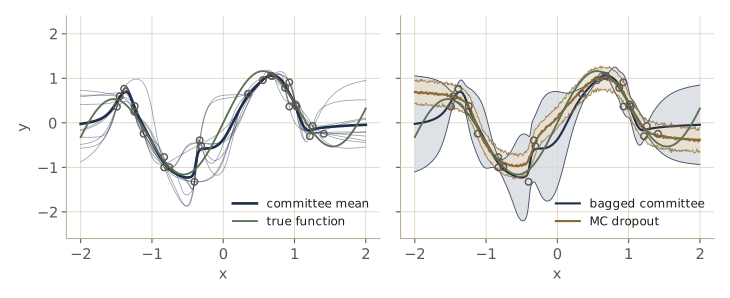
Summary
| Method | What it does | Key equation or property |
|---|---|---|
| Inductive bias | chooses among the many functions consistent with the data | no free lunch: equal off-training-set accuracy averaged over all targets |
| Data augmentation | trains on transformed copies | input noise on a linear model = weight decay with \(\lambda = N\sigma^2\) |
| Tangent propagation | penalizes output change along a transformation | \(\tfrac12\sum_n \lVert\mathbf{J}_n\boldsymbol{\tau}_n\rVert^2\) |
| Equivariant architecture | builds the symmetry into the layers | \(S(T(I)) = T(S(I))\); convolutions commute with shifts |
| Weight decay | Gaussian prior on weights | \(\widehat{w}_j = \tfrac{\lambda_j}{\lambda_j + \lambda}w^{\star}_j\), \(\gamma = \sum_j \tfrac{\lambda_j}{\lambda_j+\lambda}\) |
| Consistent regularizer | respects rescaling of inputs and targets | per-layer coefficients, biases excluded, \(\lambda_1 \to a^2\lambda_1\), \(\lambda_2 \to \lambda_2/c^2\) |
| Lasso (\(q = 1\)) | sparse weights | soft-threshold \(\operatorname{sign}(w)\max(\lvert w\rvert - \lambda/2, 0)\) |
| Early stopping | keeps the weights at the validation minimum | acts like weight decay with \(\lambda \approx 1/(\tau\eta)\) |
| Double descent | test error peaks at the interpolation threshold, then falls | minimum-norm interpolation; the peak disappears with regularization |
| Soft weight sharing | mixture-of-Gaussians prior on weights | pull \(\lambda\sum_j\gamma_j(w_i)(w_i - \mu_j)/\sigma_j^2\) |
| Residual connections | skip each block with the identity | \(\mathbf{z}_l = \mathbf{z}_{l-1} + \mathbf{F}_l(\mathbf{z}_{l-1})\); Jacobian \(\mathbf{I} + \partial\mathbf{F}_l/\partial\mathbf{z}\) |
| Committees, bagging | average several models | \(E_{\mathrm{COM}} \le E_{\mathrm{AV}}\); \(E_{\mathrm{AV}}/M\) only if errors are uncorrelated |
| Dropout | random thinning during training | inverted scaling \(1/\rho\); Monte Carlo averaging or weight scaling at test time |
Ideas to carry forward:
- A regularizer is a prior, whether it is written as a penalty, built into an architecture, or hidden in the optimizer. The most effective ones encode something true about the problem, such as smoothness or a symmetry.
- Parameter count is a poor measure of complexity. The effective number of parameters depends on \(\lambda\), on how long we train, and on the implicit preferences of the solver, which is how heavily overparameterized networks can generalize.
- Residual connections keep a direct path for signals and gradients through a deep network. That makes very deep networks trainable, smooths their gradients, and lets them behave like ensembles of shallower networks; every architecture from module 10 on uses them.
- Averaging helps in proportion to how much the members disagree. Diversity from bootstrap samples or from dropout masks is what turns one overfitting network into a better-behaved ensemble.
Exercises
- Show that the three rotations of an equilateral triangle by multiples of 120° (including the rotation by 0°) together with the three reflections through its axes form a group of six elements under composition. Is the set of rotations alone a group? Is the set of reflections alone a group? Justify each answer with the group axioms.
- For the linear model with input noise, suppose the noise has a general covariance \(\boldsymbol{\Sigma}\) instead of \(\sigma^2\mathbf{I}\). Derive the equivalent regularizer, and verify it numerically by modifying the noisy-copies experiment with a non-diagonal \(\boldsymbol{\Sigma}\).
- Draw 20 networks from the Gaussian prior of a two-layer tanh network with one input, one output, and 16 hidden units, with separate precisions for first-layer weights, first-layer biases, second-layer weights, and second-layer biases. Plot the functions on \([-2, 2]\) for several settings of the precisions, and confirm the roles described in the notes. Which precision makes the functions wiggle faster?
- For the scalar problem \(\tfrac12(w - w^{\star})^2 + \tfrac{\lambda}{2}\lvert w \rvert^q\) with \(\lambda = 1\), the notes give the minimizer for \(q = 2\) and \(q = 1\). Find it numerically on a fine grid of \(w\) for \(q = 1/2\), for \(w^{\star}\) from 0 to 3, and plot the three maps \(w^{\star} \mapsto \widehat{w}\). What is qualitatively different about \(q < 1\), and why does it make the optimization harder?
- Derive the soft-threshold formula for the lasso with orthonormal inputs by considering \(w_j > 0\), \(w_j < 0\), and \(w_j = 0\) separately. Then implement lasso by coordinate descent (update one weight at a time with the soft-threshold) and check that it agrees with
lasso_istaon the eight-input problem. - Starting from the gradient-descent recursion on a quadratic error, show that for small \(\eta\lambda_j\) the early-stopped factor \(1 - (1 - \eta\lambda_j)^{\tau}\) is close to \(1 - e^{-\eta\lambda_j\tau}\). Plot this against \(\lambda_j/(\lambda_j + \lambda)\) with \(\lambda = 1/(\tau\eta)\) as functions of \(\lambda_j\), and find the largest gap between the two curves.
- In the double-descent experiment, fix \(P = 200\) features and vary the number of training points \(N\) from 20 to 400. Plot test error against \(N\) and find a range in which more data make the minimum-norm fit worse. Explain the result in terms of the interpolation threshold.
- Show that with a single component (\(K = 1\)) whose mean is fixed at zero, the soft-sharing regularizer is weight decay plus a term that depends only on \(\sigma\), and find the \(\sigma^2\) that minimizes it for fixed weights. Then add a lower bound \(\sigma_j \ge 0.05\) to
MixturePrior(for example by writing \(\sigma_j^2 = 0.05^2 + \exp(\xi_j)\)) and check how the soft-sharing experiment changes. - For three residual blocks with linear branch functions \(\mathbf{F}_l(\mathbf{z}) = \mathbf{A}_l\mathbf{z}\), expand \(\mathbf{y}\) as a sum over paths and verify numerically with random matrices that the sum over all eight subsets of blocks reproduces the network output. How many paths of each length are there for \(L\) blocks?
- Using the committee analysis, suppose every pair of members has error correlation \(c\) and every member has the same error \(E_{\mathrm{AV}}\). Show that \(E_{\mathrm{COM}} = E_{\mathrm{AV}}\{c + (1 - c)/M\}\). Compare this prediction with the numbers printed by
committee_reportfor both committees. - Train the 1000-image MNIST network with dropout on the inputs only (\(\rho = 0.8\)), on the hidden layers only (\(\rho = 0.5\)), and on both, all with the corrupted labels. Report the test accuracy at the end of training and at the best validation epoch, and discuss which placement helps most.
- In your own words: explain to a classmate why a network with far more parameters than training points can still generalize well, using at least three ideas from this module (for example the effective number of parameters, the minimum-norm preference behind double descent, and averaging).
Going further
- C. M. Bishop and H. Bishop, Deep Learning: Foundations and Concepts (Springer, 2024), chapter 9 — the source for this module. Exercises 9.1 (groups), 9.2 (noise and weight decay), 9.4 (consistent transformations), 9.5 (penalties and constraints), 9.6 (early stopping and weight decay), 9.8–9.12 (soft weight sharing), 9.13 (unrolling residual networks), 9.14–9.17 (committees), and 9.18 (dropout for linear regression) extend the material here.
- David H. Wolpert, “The lack of a priori distinctions between learning algorithms”, Neural Computation, 1996 — the no free lunch theorems for supervised learning.
- Mikhail Belkin, Daniel Hsu, Siyuan Ma, and Soumik Mandal, “Reconciling modern machine-learning practice and the classical bias–variance trade-off”, PNAS, 2019, and Preetum Nakkiran et al., “Deep double descent: where bigger models and more data hurt”, arXiv:1912.02292 — double descent.
- Kaiming He, Xiangyu Zhang, Shaoqing Ren, and Jian Sun, “Deep residual learning for image recognition”, arXiv:1512.03385, and David Balduzzi et al., “The shattered gradients problem: if resnets are the answer, then what is the question?”, arXiv:1702.08591.
- Nitish Srivastava, Geoffrey Hinton, Alex Krizhevsky, Ilya Sutskever, and Ruslan Salakhutdinov, “Dropout: a simple way to prevent neural networks from overfitting”, JMLR, 2014; and Ilya Loshchilov and Frank Hutter, “Decoupled weight decay regularization”, arXiv:1711.05101 — AdamW.
- Related modules: Intro to ML, module 03 (regularized least squares, bias–variance), Intro to ML, module 05 (consistent priors, tangent propagation, Tikhonov), Intro to ML, module 14 (committees, bagging, boosting), and in this course module 07 (initialization and normalization) and module 10 (convolutional networks).
These notes follow the chapters of C. M. Bishop and H. Bishop, Deep Learning: Foundations and Concepts (Springer, 2024), the course text, which the authors make free to read online. The explanations, code, figures, and exercises here are written for this course; the book remains the reference, with the full derivations and many more exercises.