CSE 676 · Module 13 · Week 10
Graph Neural Networks
Graphs and permutation equivariance, neural message passing and graph convolutional networks, node, edge, and graph tasks, graph attention, over-smoothing, and geometric deep learning.
Companion reading: Bishop & Bishop, Deep Learning: Foundations and Concepts, chapter 13, “Graph Neural Networks”
By the end of this module you can
- Represent a graph by its adjacency matrix and an edge list, relabel its nodes with a permutation matrix, and state and verify the invariance and equivariance a graph network must have.
- Write a message-passing layer as Aggregate followed by Update, in matrix form and with edge lists, and prove that stacks of such layers are permutation equivariant.
- Derive the normalized propagation matrix of a graph convolutional network with self-loops, and explain its spectrum and its reading as a smoothing step.
- Compare sum, mean, and max aggregation, run the Weisfeiler–Lehman test, and exhibit pairs of different graphs that no message-passing network can tell apart.
- Train graph networks for node classification with few labels, for link prediction with held-out edges and negative sampling, and for graph classification with batched block-diagonal graphs.
- Implement graph attention with a softmax over each neighborhood, show that it reduces to mean aggregation when all scores are equal, and relate it to the transformer.
- Measure over-smoothing with the Dirichlet energy and test residual connections and layer concatenation as remedies.
- Build an E(n)-equivariant message-passing layer and verify numerically that it respects rotations, reflections, translations, and node relabeling.
Contents
- Machine learning on graphs
- Neural message passing
- General graph networks
- Summary
- Exercises
- Going further
Images and sequences are data with a fixed, regular structure: pixels on a grid, tokens on a line. Module 10 built that structure into convolutional networks, and module 12 processed sequences with attention. Much of the world’s data has structure that is not a grid or a line. A molecule is a set of atoms joined by bonds; a citation network is a set of papers joined by references; a road map is a set of junctions joined by roads. The natural description of such data is a graph, a set of objects together with the pairwise relations between them, and this module is about networks that take graphs as input.
The central difficulty is that a graph has no preferred order for its nodes. To store a graph in a computer we must number the nodes, but any numbering describes the same graph, and a prediction that changed with the numbering would be meaningless. Module 09 introduced invariance and equivariance as properties to build into an architecture; here the symmetry is the group of all node relabelings, and we will build networks that respect it exactly. The construction that does this, neural message passing, lets every node repeatedly collect information from its neighbors, with the same learned functions at every node. We derive it from the convolutional layer, implement it with plain PyTorch tensors (dense matrices for small graphs, edge lists for anything larger), and use it for the three kinds of task that graphs pose: predicting properties of nodes, of edges, and of whole graphs.
The chapter of Bishop & Bishop behind this module is short, and graph representation learning is an active research area, so the notes go further than the book in a few places where the material is well established: how much structure message passing can see (the Weisfeiler–Lehman test), how link prediction is evaluated, and how over-smoothing can be measured. All code runs on a CPU in well under a minute per section; the graphs are small and synthetic so that we know the truth behind every result.
import math
import time
import collections
import numpy as np
import networkx as nx                     # only to build and check small graphs
import torch
import torch.nn as nn
import torch.nn.functional as F

np.set_printoptions(precision=4, suppress=True)
rng = np.random.default_rng(13)
torch.manual_seed(13)
Machine learning on graphs
A graph consists of nodes (also called vertices) and edges (also called links) that join pairs of nodes. Both can carry data. In a molecule, a node’s data is its atom type and an edge’s data is the bond type. In a road network, an edge can carry the length of the road. In a social network, a node’s data can be a person’s profile and an edge can record when two people connected.
Learning problems on graphs fall into three groups, according to what we want to predict.
- Node-level tasks predict a property of each node: the research field of each paper in a citation network, or whether each account in a social network is a person or a bot.
- Edge-level tasks predict a property of pairs of nodes. The most common is link prediction (also called graph completion): given the edges we know, which missing edges are likely to exist? Recommending products to customers, or suggesting which proteins might interact, are examples.
- Graph-level tasks predict a property of a whole graph from a data set of graphs: whether a molecule is toxic, or how well it dissolves in water. These are graph classification and graph regression problems.
The node and edge tasks usually come with a twist that we have not met before. Often there is only one graph, say a social network with millions of accounts, and we have labels for a few hundred of them. We see the whole graph during training, including the unlabeled nodes and their connections, and we want labels for the unlabeled nodes of this same graph. That setting is called transductive: training and prediction happen on one fixed set of objects, and the unlabeled nodes help during training because they carry information along the edges. It is a form of semi-supervised learning. The more familiar setting, in which the test objects are new ones not seen during training (a new molecule, a new user who joins later), is inductive. Graph-level tasks are always inductive.
Beyond solving one task, a network trained on graphs produces a vector for every node (and possibly every edge and graph) that summarizes its neighborhood. Learning such vectors so that they are useful for many downstream tasks is called graph representation learning. The vectors are called embeddings, as for the tokens of a transformer: every node starts with an embedding given by its observed data, and each layer of the network refines every embedding using the embeddings of its neighbors, much as each transformer layer refines a token’s embedding using the other tokens in the context.
Graph properties
We write a graph as \(G = (\mathcal{V}, \mathcal{E})\), with node set \(\mathcal{V}\) and edge set \(\mathcal{E}\). The nodes are numbered \(n = 1, \dots, N\), and \((n, m) \in \mathcal{E}\) means there is an edge from node \(n\) to node \(m\). Two nodes joined by an edge are neighbors, and the set of neighbors of node \(n\) is its neighborhood \(\mathcal{N}(n)\). The number of neighbors, \(\lvert \mathcal{N}(n) \rvert\), is the degree of the node.
Graphs come in several varieties.
| Kind | What it means | Example |
|---|---|---|
| undirected | every edge goes both ways | friendship, chemical bonds, roads |
| directed | \((n, m)\) does not imply \((m, n)\) | hyperlinks, citations, “follows” |
| weighted | edges carry a number | travel time, interaction strength |
| attributed | nodes and/or edges carry feature vectors | atoms with types, bonds with types |
| multi-relational | several kinds of nodes or edges | a knowledge graph of people, papers, and venues |
| with self-loops | a node may link to itself | a web page that links to itself |
We work mainly with simple graphs: undirected, no self-loops, and no two nodes joined by more than one edge. The ideas carry over to the other kinds with small changes (separate weights per edge type, a direction flag, an edge feature). Each node \(n\) carries a \(D\)-dimensional feature vector \(\mathbf{x}_n\), and we stack these as the rows of the node feature matrix \(\mathbf{X}\) of size \(N \times D\), exactly like a data matrix, one row per node.
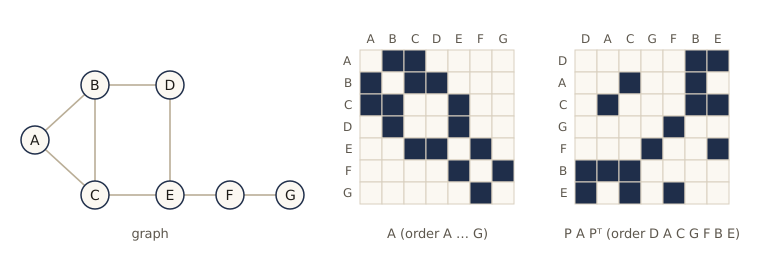
Our running example is a small graph with seven nodes, labeled A to G, and eight edges: a triangle A–B–C, a square B–D–E–C that shares the edge B–C with it, and a tail E–F–G.
names = ["A", "B", "C", "D", "E", "F", "G"]
edge_list = [(0, 1), (0, 2), (1, 2), (1, 3), (2, 4), (3, 4), (4, 5), (5, 6)]

def adjacency(edge_list, N):
    """Symmetric 0/1 adjacency matrix of an undirected simple graph."""
    A = torch.zeros(N, N)
    for n, m in edge_list:
        A[n, m] = A[m, n] = 1.0
    return A

N = len(names)
A = adjacency(edge_list, N)
print(A.int())
deg = A.sum(1)
print("degrees:", dict(zip(names, deg.int().tolist())))
print("neighbors of C:", [names[m] for m in A[2].nonzero().flatten().tolist()])
tensor([[0, 1, 1, 0, 0, 0, 0],
        [1, 0, 1, 1, 0, 0, 0],
        [1, 1, 0, 0, 1, 0, 0],
        [0, 1, 0, 0, 1, 0, 0],
        [0, 0, 1, 1, 0, 1, 0],
        [0, 0, 0, 0, 1, 0, 1],
        [0, 0, 0, 0, 0, 1, 0]], dtype=torch.int32)
degrees: {'A': 2, 'B': 3, 'C': 3, 'D': 2, 'E': 3, 'F': 2, 'G': 1}
neighbors of C: ['A', 'B', 'E']
Adjacency matrix
The matrix printed above is the adjacency matrix \(\mathbf{A}\) of the graph: an \(N \times N\) matrix with \(A_{nm} = 1\) if there is an edge from \(n\) to \(m\) and \(A_{nm} = 0\) otherwise. For an undirected graph it is symmetric, \(A_{nm} = A_{mn}\), and for a simple graph its diagonal is zero. Row \(n\) lists the neighbors of node \(n\), so the degree of node \(n\) is the row sum \(\sum_m A_{nm}\). We collect the degrees on the diagonal of the degree matrix \(\mathbf{D} = \operatorname{diag}(\mathbf{A}\mathbf{1})\), where \(\mathbf{1}\) is the vector of ones. (It is bold, to keep it apart from the feature dimension \(D\).)
Powers of \(\mathbf{A}\) count walks. A walk of length \(k\) is a sequence of \(k\) edges in which each edge starts where the previous one ended (nodes may repeat). Expanding the matrix product,
\[(\mathbf{A}^2)_{nm} = \sum_{j} A_{nj} A_{jm},\]and the term \(A_{nj}A_{jm}\) is 1 exactly when \(n \to j \to m\) is a walk, so \((\mathbf{A}^2)_{nm}\) counts walks of length 2 from \(n\) to \(m\); by induction \((\mathbf{A}^k)_{nm}\) counts walks of length \(k\). Two consequences: the diagonal of \(\mathbf{A}^2\) is the degree (a walk of length 2 from \(n\) back to \(n\) goes out along an edge and comes straight back), and \(\operatorname{tr}(\mathbf{A}^3)/6\) is the number of triangles (each triangle gives six closed walks of length 3: three starting points and two directions).
For anything but small graphs we do not store \(\mathbf{A}\) as a dense matrix. Real graphs are sparse: the number of edges grows roughly like \(N\), not \(N^2\). The standard compact form is the edge list (called an edge index in graph libraries): a \(2 \times E\) integer array whose columns are the directed pairs \((m, n)\), with each undirected edge stored in both directions. We will write every layer in both forms, dense for clarity and edge list for scale.
A2, A3 = A @ A, A @ A @ A
print("diagonal of A^2:", torch.diagonal(A2).int().tolist(), "(= degrees)")
print(f"walks of length 3 from A to E: {A3[0, 4].item():.0f}")
print(f"triangles: tr(A^3)/6 = {torch.trace(A3).item() / 6:.0f}")

edge_index = A.nonzero().T               # (2, E): row 0 = source m, row 1 = target n
print("edge list shape", tuple(edge_index.shape), " first columns:", edge_index[:, :4].tolist())
N_big, mean_degree = 10**6, 100          # a large social network, for scale
print(f"dense adjacency: {N_big**2:.1e} entries   edge list: {2 * N_big * mean_degree:.1e} entries")
diagonal of A^2: [2, 3, 3, 2, 3, 2, 1] (= degrees)
walks of length 3 from A to E: 2
triangles: tr(A^3)/6 = 1
edge list shape (2, 16)  first columns: [[0, 0, 1, 1], [1, 2, 0, 2]]
dense adjacency: 1.0e+12 entries   edge list: 2.0e+08 entries
Permutation equivariance
The adjacency matrix depends on the order in which we numbered the nodes. Why not flatten \(\mathbf{A}\) into a vector of \(N^2\) numbers and feed it, together with \(\mathbf{X}\), to an ordinary network? Because the same graph has up to \(N!\) different adjacency matrices, one for each numbering, and a network on the flattened matrix would give each of them a different output. It could learn to ignore the numbering only by seeing an astronomical number of relabeled copies of every graph. The symmetry has to be built into the architecture.
A relabeling of the nodes is a permutation \(\pi\) of \(\{1, \dots, N\}\). We describe it with a permutation matrix \(\mathbf{P}\): row \(n\) of \(\mathbf{P}\) is the unit row vector \(\mathbf{u}_{\pi(n)}^{\mathrm{T}}\), which has a 1 in position \(\pi(n)\) and zeros elsewhere. Every row and every column of \(\mathbf{P}\) contains exactly one 1, and \(\mathbf{P}^{\mathrm{T}}\mathbf{P} = \mathbf{P}\mathbf{P}^{\mathrm{T}} = \mathbf{I}\). Row \(n\) of \(\mathbf{P}\mathbf{X}\) is \(\mathbf{u}_{\pi(n)}^{\mathrm{T}}\mathbf{X} = \mathbf{x}_{\pi(n)}^{\mathrm{T}}\), so the new node \(n\) is the old node \(\pi(n)\), and
\[\widetilde{\mathbf{X}} = \mathbf{P}\mathbf{X}, \qquad \widetilde{\mathbf{A}} = \mathbf{P}\mathbf{A}\mathbf{P}^{\mathrm{T}},\]since the adjacency matrix has a row and a column for every node, and we relabel both: \(\widetilde{A}_{nm} = A_{\pi(n)\pi(m)}\).
Now we can say precisely what we want from a network. A prediction about the whole graph must not change under relabeling. A function \(y(\mathbf{X}, \mathbf{A})\) is permutation invariant if
\[y(\mathbf{P}\mathbf{X}, \mathbf{P}\mathbf{A}\mathbf{P}^{\mathrm{T}}) = y(\mathbf{X}, \mathbf{A}) \quad \text{for every permutation matrix } \mathbf{P}.\]A prediction for each node must move with its node: if we relabel the nodes, the rows of the output should be relabeled the same way. A function \(\mathbf{Y}(\mathbf{X}, \mathbf{A})\) with one output row per node is permutation equivariant if
\[\mathbf{Y}(\mathbf{P}\mathbf{X}, \mathbf{P}\mathbf{A}\mathbf{P}^{\mathrm{T}}) = \mathbf{P}\,\mathbf{Y}(\mathbf{X}, \mathbf{A}) \quad \text{for every permutation matrix } \mathbf{P}.\]These are the definitions of module 09 with the relabeling as the transformation: \(\mathbf{P}\) acts on the input by relabeling both \(\mathbf{X}\) and \(\mathbf{A}\), and on the output by relabeling its rows. Let us relabel our example graph with a random permutation and check that nothing but the numbering has changed, and that a network on the flattened adjacency matrix does not respect it.
perm = torch.from_numpy(rng.permutation(N))
P = torch.eye(N)[perm]                                # row n of P is u_{pi(n)}^T
X = torch.from_numpy(rng.normal(size=(N, 3))).float()
X_t, A_t = P @ X, P @ A @ P.T
print("new order of the old nodes:", [names[i] for i in perm.tolist()])
print("P X relabels the rows:", torch.equal(X_t, X[perm]),
      "   P A P^T relabels rows and columns:", torch.equal(A_t, A[perm][:, perm]))
print("same graph (isomorphic):",
      nx.is_isomorphic(nx.from_numpy_array(A.numpy()), nx.from_numpy_array(A_t.numpy())))

flat_net = nn.Sequential(nn.Linear(N * N, 16), nn.ReLU(), nn.Linear(16, 1))
with torch.no_grad():
    print(f"network on flattened A: {flat_net(A.flatten()).item():.4f} "
          f"vs {flat_net(A_t.flatten()).item():.4f} after relabeling")
print(f"numberings of a 7-node graph: {math.factorial(7)};"
      f"  of a 30-node graph: {math.factorial(30):.1e}")
new order of the old nodes: ['D', 'A', 'C', 'G', 'F', 'B', 'E']
P X relabels the rows: True    P A P^T relabels rows and columns: True
same graph (isomorphic): True
network on flattened A: -0.5967 vs -0.3669 after relabeling
numberings of a 7-node graph: 5040;  of a 30-node graph: 2.7e+32
Neural message passing
What should a layer for graphs look like? It should be equivariant, so that a stack of layers is equivariant too (we prove this below), and a final invariant step can then produce graph-level outputs. It should be a flexible, differentiable function with learnable parameters, so that we can train it by gradient descent. It should accept graphs of any size, since molecules have different numbers of atoms, and it should scale to graphs with millions of nodes. Parameter sharing is the key to all four requirements, just as it was for convolutional layers.
Convolutional filters
An image is itself a graph: the nodes are the pixels, and each pixel is joined to its eight surrounding pixels (horizontal, vertical, and diagonal neighbors). A convolutional layer with a \(3 \times 3\) filter computes, at pixel \(i\) of layer \(l+1\),
\[z_i^{(l+1)} = f\Big( \sum_{j} w_j z_j^{(l)} + b \Big),\]where the sum runs over the nine pixels of the patch centered at \(i\), \(f\) is an activation function such as the ReLU, and the same weights \(w_j\) and bias \(b\) are used at every position.
This formula cannot be used on a general graph as it stands. Each weight \(w_j\) belongs to a direction (up-left, up, up-right, and so on), and in a graph there are no directions: the neighbors of a node form an unordered set, and their numbering is arbitrary. The fix is to give all neighbors the same weight and to keep one separate weight for the center pixel:
\[z_i^{(l+1)} = f\Big( w_{\mathrm{neigh}} \sum_{j \in \mathcal{N}(i)} z_j^{(l)} + w_{\mathrm{self}}\, z_i^{(l)} + b \Big).\]Read as a graph computation, each neighbor sends its value as a message to node \(i\); the messages are summed, which does not depend on their order; and the sum is combined with node \(i\)’s own value and passed through \(f\). The same three parameters are used at every node. If we relabel the nodes, every node still receives the same messages from the same neighbors and computes the same result; only the positions in the output list change. That is equivariance, and it rests entirely on the sharing of \(w_{\mathrm{neigh}}\), \(w_{\mathrm{self}}\), and \(b\) across nodes.
We can check the correspondence directly: on the grid graph of a \(6 \times 6\) image, the message-passing formula equals a convolution whose kernel has \(w_{\mathrm{self}}\) in the middle and \(w_{\mathrm{neigh}}\) in the other eight places (with zero padding at the border, where pixels have fewer neighbors).
def grid_adjacency(S):
    """8-neighbor grid graph of an S x S image, pixels numbered row by row."""
    A = torch.zeros(S * S, S * S)
    for i in range(S):
        for j in range(S):
            for di in (-1, 0, 1):
                for dj in (-1, 0, 1):
                    if (di or dj) and 0 <= i + di < S and 0 <= j + dj < S:
                        A[i * S + j, (i + di) * S + (j + dj)] = 1.0
    return A

side = 6
A_grid = grid_adjacency(side)
img = torch.from_numpy(rng.normal(size=(side, side))).float()
w_neigh, w_self, b = 0.3, -1.2, 0.1
kernel = torch.full((3, 3), w_neigh)
kernel[1, 1] = w_self
conv_out = F.conv2d(img[None, None], kernel[None, None], padding=1)[0, 0] + b
mp_out = w_neigh * (A_grid @ img.flatten()) + w_self * img.flatten() + b
gap = (conv_out.flatten() - mp_out).abs().max().item()
print(f"max difference, convolution vs message passing: {gap:.1e}")
print("degrees on the grid graph:", sorted(set(A_grid.sum(1).int().tolist())))
max difference, convolution vs message passing: 2.4e-07
degrees on the grid graph: [3, 5, 8]
The general convolution has nine free weights per filter and the message-passing version only two, so we have given something up: a graph layer cannot tell its neighbors apart by position. On a grid that is a real loss, which is why convolutional networks remain the right tool for images. On a general graph there is nothing to lose, because there are no positions.
Graph convolutional networks
We now turn the example into a general layer. Each node \(n\) has an embedding vector \(\mathbf{h}_n^{(l)}\) at layer \(l\), initialized with its features, \(\mathbf{h}_n^{(0)} = \mathbf{x}_n\). A message-passing layer does two things at every node, with functions shared across nodes.
- Aggregate: combine the embeddings of the neighbors into one vector, \(\mathbf{z}_n^{(l)} = \operatorname{Aggregate}\big(\{\mathbf{h}_m^{(l)} : m \in \mathcal{N}(n)\}\big)\). The aggregation must not depend on the order of the neighbors and must work for any number of them.
- Update: combine the aggregated message with the node’s own embedding, \(\mathbf{h}_n^{(l+1)} = \operatorname{Update}\big(\mathbf{h}_n^{(l)}, \mathbf{z}_n^{(l)}\big)\).
A network is a stack of \(L\) such layers, usually with separate parameters in each layer. This framework is the message-passing neural network (Gilmer et al., 2017), and nearly every graph network in use is an instance of it. The simplest choice follows the image example: sum the neighbors, and combine linearly before a nonlinearity,
\[\mathbf{h}_n^{(l+1)} = f\Big( \mathbf{W}_{\mathrm{self}}\, \mathbf{h}_n^{(l)} + \mathbf{W}_{\mathrm{neigh}} \sum_{m \in \mathcal{N}(n)} \mathbf{h}_m^{(l)} + \mathbf{b} \Big).\]Matrix form. Stack the embeddings as the rows of \(\mathbf{H}\) (\(N \times D\)). Row \(n\) of \(\mathbf{A}\mathbf{H}\) is \(\sum_m A_{nm} \mathbf{h}_m^{\mathrm{T}} = \sum_{m \in \mathcal{N}(n)} \mathbf{h}_m^{\mathrm{T}}\), so the aggregation for all nodes at once is the product \(\mathbf{Z} = \mathbf{A}\mathbf{H}\). With the weights acting on row vectors from the right (the PyTorch convention), the whole layer is
\[\mathbf{H}^{(l+1)} = f\big( \mathbf{A}\mathbf{H}^{(l)}\mathbf{W}_{\mathrm{neigh}} + \mathbf{H}^{(l)}\mathbf{W}_{\mathrm{self}} + \mathbf{1}\mathbf{b}^{\mathrm{T}} \big).\]Equivariance, proved. Call the right-hand side \(F(\mathbf{H}, \mathbf{A})\). Substituting the relabeled inputs and using \(\mathbf{P}^{\mathrm{T}}\mathbf{P} = \mathbf{I}\) and \(\mathbf{P}\mathbf{1} = \mathbf{1}\),
\[\begin{aligned} F(\mathbf{P}\mathbf{H}, \mathbf{P}\mathbf{A}\mathbf{P}^{\mathrm{T}}) &= f\big( \mathbf{P}\mathbf{A}\mathbf{P}^{\mathrm{T}}\mathbf{P}\mathbf{H}\mathbf{W}_{\mathrm{neigh}} + \mathbf{P}\mathbf{H}\mathbf{W}_{\mathrm{self}} + \mathbf{P}\mathbf{1}\mathbf{b}^{\mathrm{T}} \big) \\ &= f\big( \mathbf{P}\,( \mathbf{A}\mathbf{H}\mathbf{W}_{\mathrm{neigh}} + \mathbf{H}\mathbf{W}_{\mathrm{self}} + \mathbf{1}\mathbf{b}^{\mathrm{T}} ) \big) = \mathbf{P}\, F(\mathbf{H}, \mathbf{A}), \end{aligned}\]where the last step uses that \(f\) acts element by element, so it does not care in which order the rows come. For a stack of layers, \(\mathbf{H}^{(l)} = F_l(\mathbf{H}^{(l-1)}, \mathbf{A})\), induction does the rest: if \(\mathbf{P}\mathbf{H}^{(l-1)}\) is what layer \(l-1\) produces from the relabeled graph, then layer \(l\) produces \(F_l(\mathbf{P}\mathbf{H}^{(l-1)}, \mathbf{P}\mathbf{A}\mathbf{P}^{\mathrm{T}}) = \mathbf{P}\mathbf{H}^{(l)}\). So the whole network is equivariant. Summing the rows of the final layer, \(\mathbf{1}^{\mathrm{T}}\mathbf{H}^{(L)}\), gives an invariant, because \(\mathbf{1}^{\mathrm{T}}\mathbf{P} = \mathbf{1}^{\mathrm{T}}\).
With an edge list the aggregation is a scatter-add: gather the source embeddings \(\mathbf{h}_m\) of all edges, and add each into the row of its target \(n\). In PyTorch that is index_add_. Both forms give the same numbers; the edge-list form costs time and memory proportional to the number of edges.
def aggregate_sum(H, edge_index):
    """z_n = sum of h_m over edges (m -> n), as a scatter-add over the edge list."""
    src, dst = edge_index
    return torch.zeros_like(H).index_add_(0, dst, H[src])

class MPLayer(nn.Module):
    """h_n' = f(W_self h_n + W_neigh sum_{m in N(n)} h_m + b), dense adjacency."""
    def __init__(self, d_in, d_out):
        super().__init__()
        self.lin_self = nn.Linear(d_in, d_out)                 # W_self and b
        self.lin_neigh = nn.Linear(d_in, d_out, bias=False)    # W_neigh
    def forward(self, H, A):
        return torch.relu(self.lin_self(H) + self.lin_neigh(A @ H))

print(f"dense A @ X vs scatter-add over the edge list: "
      f"{(A @ X - aggregate_sum(X, edge_index)).abs().max().item():.1e}")

torch.manual_seed(13)
layers = nn.ModuleList([MPLayer(3, 8), MPLayer(8, 8)])
def mp_net(H, A):
    for layer in layers:
        H = layer(H, A)
    return H

with torch.no_grad():
    out, out_t = mp_net(X, A), mp_net(P @ X, P @ A @ P.T)
    print(f"equivariance: max |Y(PX, PAP^T) - P Y(X, A)| = "
          f"{(out_t - P @ out).abs().max().item():.1e}"
          f"   (outputs are of size {out.abs().max().item():.2f})")
    print(f"invariance of the sum readout: {(out_t.sum(0) - out.sum(0)).abs().max().item():.1e}")
dense A @ X vs scatter-add over the edge list: 0.0e+00
equivariance: max |Y(PX, PAP^T) - P Y(X, A)| = 2.4e-07   (outputs are of size 3.83)
invariance of the sum readout: 9.5e-07
The differences are at the level of floating-point round-off: summing the same numbers in a different order can change the last bit.
The graph convolutional network. A popular special case is the graph convolutional network (GCN) of Kipf and Welling (2017). Start from the layer above and make two simplifications. First, share one matrix between the node and its neighbors, \(\mathbf{W}_{\mathrm{self}} = \mathbf{W}_{\mathrm{neigh}} = \mathbf{W}\). The node’s own embedding then enters exactly like a neighbor’s, which is the same as adding a self-loop to every node: with \(\hat{\mathbf{A}} = \mathbf{A} + \mathbf{I}\),
\[\mathbf{H}^{(l+1)} = f\big( \hat{\mathbf{A}}\mathbf{H}^{(l)}\mathbf{W} + \mathbf{1}\mathbf{b}^{\mathrm{T}} \big).\]Second, fix the scale. Multiplying by \(\hat{\mathbf{A}}\) adds up \(\hat{d}_n = \lvert \mathcal{N}(n) \rvert + 1\) vectors at node \(n\), so a hub with a thousand neighbors receives a message a thousand times larger than a node with one. Worse, the largest eigenvalue of \(\hat{\mathbf{A}}\) is at least the average degree plus one, so applying it layer after layer makes embeddings grow geometrically. There are two natural normalizations. Dividing by the degree, \(\hat{\mathbf{D}}^{-1}\hat{\mathbf{A}}\), where \(\hat{\mathbf{D}} = \operatorname{diag}(\hat{\mathbf{A}}\mathbf{1})\), averages over the node and its neighbors; the matrix is row-stochastic (rows are nonnegative and sum to one), so its eigenvalues lie in \([-1, 1]\). The GCN uses the symmetric version
\[\mathbf{S} = \hat{\mathbf{D}}^{-1/2}\hat{\mathbf{A}}\hat{\mathbf{D}}^{-1/2}, \qquad S_{nm} = \frac{\hat{A}_{nm}}{\sqrt{\hat{d}_n \hat{d}_m}},\]which weights the message from \(m\) to \(n\) by \(1/\sqrt{\hat{d}_n \hat{d}_m}\): a message from a well-connected neighbor counts less, because that neighbor is sending the same message to many nodes. \(\mathbf{S}\) is similar to the row-stochastic matrix, \(\mathbf{S} = \hat{\mathbf{D}}^{1/2}(\hat{\mathbf{D}}^{-1}\hat{\mathbf{A}})\hat{\mathbf{D}}^{-1/2}\), so it has the same eigenvalues, all in \([-1, 1]\), with the largest equal to 1 and eigenvector \(\hat{\mathbf{D}}^{1/2}\mathbf{1}\). Because it is also symmetric, it cannot amplify any vector: \(\lVert \mathbf{S}\mathbf{v} \rVert \le \lVert \mathbf{v} \rVert\). The GCN layer is
Result. Graph convolutional layer (Kipf and Welling):
\[\mathbf{H}^{(l+1)} = f\big( \mathbf{S}\,\mathbf{H}^{(l)}\mathbf{W}^{(l)} \big), \qquad \mathbf{S} = \hat{\mathbf{D}}^{-1/2}(\mathbf{A} + \mathbf{I})\hat{\mathbf{D}}^{-1/2}.\]Per node: \(\mathbf{h}_n^{(l+1)} = f\big( \sum_{m \in \mathcal{N}(n) \cup \{n\}} \mathbf{W}^{(l)\mathrm{T}}\mathbf{h}_m^{(l)} / \sqrt{\hat{d}_n \hat{d}_m} \big)\). A bias is often added.
Kipf and Welling arrived at this layer from a different direction, as a first-order approximation of filters defined through the eigenvectors of the graph Laplacian, and found that adding the self-loops before normalizing (they called it a renormalization) made training more stable. The next cell shows why the normalization matters on a graph with very uneven degrees: a preferential-attachment graph of 200 nodes, whose degrees range from 2 to several dozen. We print the range of eigenvalues of each candidate matrix and the norm of a random vector after ten applications.
def gcn_norm(A):
    """S = D^-1/2 (A + I) D^-1/2 with D the degree matrix of A + I."""
    A_hat = A + torch.eye(len(A))
    d_hat = A_hat.sum(1)
    return A_hat / torch.sqrt(d_hat[:, None] * d_hat[None, :])

A_ba = torch.tensor(nx.to_numpy_array(nx.barabasi_albert_graph(200, 2, seed=13)),
                    dtype=torch.float32)
d_ba = A_ba.sum(1)
print(f"degrees from {d_ba.min().item():.0f} to {d_ba.max().item():.0f}")
v0 = torch.from_numpy(rng.normal(size=(200, 1))).float()
v0 = v0 / v0.norm()
candidates = [("A + I", A_ba + torch.eye(200)),
              ("D^-1 A (mean)", A_ba / d_ba[:, None]),
              ("D^-1/2 A D^-1/2", A_ba / torch.sqrt(d_ba[:, None] * d_ba[None, :])),
              ("S (GCN)", gcn_norm(A_ba))]
for name, M in candidates:
    ev = torch.linalg.eigvals(M).real
    v = v0.clone()
    for _ in range(10):
        v = M @ v
    print(f"{name:16s} eigenvalues in [{ev.min().item():6.3f}, {ev.max().item():6.3f}]"
          f"   norm after 10 steps {v.norm().item():.2e}")
degrees from 2 to 39
A + I            eigenvalues in [-5.543,  9.282]   norm after 10 steps 1.50e+08
D^-1 A (mean)    eigenvalues in [-0.837,  1.000]   norm after 10 steps 9.81e-02
D^-1/2 A D^-1/2  eigenvalues in [-0.837,  1.000]   norm after 10 steps 4.42e-02
S (GCN)          eigenvalues in [-0.476,  1.000]   norm after 10 steps 4.65e-02
Without normalization a unit vector grows by eight orders of magnitude in ten steps; the normalized matrices keep it of order one. Adding the self-loops before normalizing also pulls the smallest eigenvalue away from \(-1\) (here from about \(-0.84\) to about \(-0.48\)). Eigenvalues near \(-1\) correspond to patterns that flip sign between neighbors, and repeated multiplication makes them oscillate from layer to layer; the self-loops damp them.
There is a useful way to read \(\mathbf{S}\). Define the normalized graph Laplacian \(\hat{\mathbf{L}} = \mathbf{I} - \mathbf{S}\). For a vector \(\mathbf{x}\) with one number per node, a short calculation (expand the square and use \(\sum_m \hat{A}_{nm} = \hat{d}_n\)) gives
\[\mathbf{x}^{\mathrm{T}}\hat{\mathbf{L}}\mathbf{x} = \frac{1}{2}\sum_{n,m} \hat{A}_{nm} \Big( \frac{x_n}{\sqrt{\hat{d}_n}} - \frac{x_m}{\sqrt{\hat{d}_m}} \Big)^2 .\]This is the Dirichlet energy of \(\mathbf{x}\) on the graph: it is small when the (degree-scaled) values at neighboring nodes are close. The gradient of \(\tfrac{1}{2}\mathbf{x}^{\mathrm{T}}\hat{\mathbf{L}}\mathbf{x}\) is \(\hat{\mathbf{L}}\mathbf{x}\) (the matrix is symmetric), so \(\mathbf{S}\mathbf{x} = \mathbf{x} - \hat{\mathbf{L}}\mathbf{x}\) is one step of gradient descent on half the Dirichlet energy, with step size 1. The propagation in a GCN is a smoothing step: it makes each node’s embedding more like its neighbors’. That is exactly what we want when neighbors tend to share labels, and it is also the source of over-smoothing, which we measure later in this module.
For large sparse graphs we never form \(\mathbf{S}\) densely. Each edge \((m, n)\), including the self-loops, gets the weight \(1/\sqrt{\hat{d}_n \hat{d}_m}\), and the product becomes a weighted scatter-add. PyTorch’s sparse matrices do the same thing, and serve as a cross-check.
def gcn_edges(edge_index, N):
    """Edge list with self-loops, and the GCN weight 1/sqrt(d_n d_m) of every edge."""
    loops = torch.arange(N)
    ei = torch.cat([edge_index, torch.stack([loops, loops])], 1)
    d_hat = torch.zeros(N).index_add_(0, ei[1], torch.ones(ei.shape[1]))
    return ei, 1.0 / torch.sqrt(d_hat[ei[0]] * d_hat[ei[1]])

def propagate(H, ei, weight):
    """Row n of the result = sum over edges (m -> n) of weight * h_m."""
    return torch.zeros_like(H).index_add_(0, ei[1], weight[:, None] * H[ei[0]])

ei_hat, w_hat = gcn_edges(edge_index, N)
# entry (n, m) of S for the edge m -> n
S_sparse = torch.sparse_coo_tensor(ei_hat.flip(0), w_hat, (N, N), check_invariants=False)
dense, scatter, sparse = gcn_norm(A) @ X, propagate(X, ei_hat, w_hat), torch.sparse.mm(S_sparse, X)
print(f"dense vs scatter: {(dense - scatter).abs().max().item():.1e}"
      f"   dense vs torch.sparse: {(dense - sparse).abs().max().item():.1e}")
dense vs scatter: 6.0e-08 dense vs torch.sparse: 3.0e-08
Aggregation operators
The aggregation step must be a function of a multiset of vectors (a set that may contain repeats, since two neighbors can have equal embeddings): it may not depend on their order, and it must accept any number of them. The common choices, all applied element by element:
| Aggregation | \(\mathbf{z}_n\) | Notes |
|---|---|---|
| sum | \(\sum_{m \in \mathcal{N}(n)} \mathbf{h}_m\) | keeps the count of neighbors; scale grows with degree |
| mean | \(\frac{1}{\lvert \mathcal{N}(n) \rvert}\sum_{m \in \mathcal{N}(n)} \mathbf{h}_m\) | scale-free; loses the count |
| symmetric (GCN) | \(\sum_{m \in \mathcal{N}(n)} \mathbf{h}_m / \sqrt{\lvert \mathcal{N}(n) \rvert\, \lvert \mathcal{N}(m) \rvert}\) | between the two; also discounts busy neighbors |
| max (or min) | \(\max_{m \in \mathcal{N}(n)} \mathbf{h}_m\) | picks out the most extreme neighbor in each coordinate |
The sum is the most informative of these. On a social network, however, degrees can range over several orders of magnitude, and a sum then produces messages of wildly different sizes; the mean fixes the scale at the price of forgetting how many neighbors there were. Which matters more depends on whether the node features or the graph structure carry the signal.
None of these aggregations has learnable parameters. A learnable one transforms each neighbor’s embedding by a small network before summing, and transforms the sum by another network:
\[\mathbf{z}_n = \mathrm{MLP}_{\theta}\Big( \sum_{m \in \mathcal{N}(n)} \mathrm{MLP}_{\phi}(\mathbf{h}_m) \Big).\]With the two networks shared across nodes, this is still permutation invariant. It is also, in a precise sense, as general as possible: Zaheer et al. (2017) showed that, under mild technical conditions, functions of this form can represent any permutation-invariant function of a set. Applied to a graph with no edges, where each node aggregates over all the other elements of a set, it is the deep sets architecture for learning on unordered sets such as point clouds.
The next cell makes the differences concrete with neighborhoods of one-dimensional embeddings: four pairs of different multisets, each summarized by the sum, the mean, the max, and the sum of a fixed nonlinear transform \(\phi(v) = v^2\) of the elements (a stand-in for \(\mathrm{MLP}_{\phi}\)). It then checks that a small deep-set network, with random weights, is unchanged by shuffling its inputs.
def aggregations(values):
    v = torch.tensor(values, dtype=torch.float32)
    return (f"{str(values):22s}{v.sum().item():6.1f}{v.mean().item():7.2f}{v.max().item():6.1f}"
            f"{(v ** 2).sum().item():9.1f}")

pairs = [([1., 1.], [1.]), ([1., 2.], [1., 1., 2., 2.]),
         ([0., 2.], [1., 1.]), ([0., 3.], [1., 2., 3.])]
print(f"{'neighbor embeddings':22s}{'sum':>6s}{'mean':>7s}{'max':>6s}{'sum v^2':>9s}")
for a, b in pairs:
    print(aggregations(a))
    print(aggregations(b))
    print()

torch.manual_seed(13)
mlp_phi = nn.Sequential(nn.Linear(2, 16), nn.ReLU(), nn.Linear(16, 16))
mlp_theta = nn.Sequential(nn.Linear(16, 16), nn.ReLU(), nn.Linear(16, 1))
def deep_set(V):
    return mlp_theta(mlp_phi(V).sum(0))
V = torch.from_numpy(rng.normal(size=(5, 2))).float()
with torch.no_grad():
    print(f"deep set on 5 vectors: {deep_set(V).item():.4f}   shuffled: "
          f"{deep_set(V[torch.randperm(5)]).item():.4f}"
          f"   on 3 of them: {deep_set(V[:3]).item():.4f}")
neighbor embeddings      sum   mean   max  sum v^2
[1.0, 1.0]               2.0   1.00   1.0      2.0
[1.0]                    1.0   1.00   1.0      1.0

[1.0, 2.0]               3.0   1.50   2.0      5.0
[1.0, 1.0, 2.0, 2.0]     6.0   1.50   2.0     10.0

[0.0, 2.0]               2.0   1.00   2.0      4.0
[1.0, 1.0]               2.0   1.00   1.0      2.0

[0.0, 3.0]               3.0   1.50   3.0      9.0
[1.0, 2.0, 3.0]          6.0   2.00   3.0     14.0

deep set on 5 vectors: 0.8920   shuffled: 0.8920   on 3 of them: 0.2479
Each block of two rows is a pair of neighborhoods. In the first pair, a node with two neighbors of embedding 1 and a node with one such neighbor look identical to mean and max; the sum sees the difference. The second pair fools mean and max again (doubling the count of every neighbor changes neither). In the third pair, the mean and the plain sum are both fooled (\(0 + 2 = 1 + 1\)), while the max is not. In the last, the max is fooled and the mean is not. The only summary that separates all four pairs is the sum of transformed elements, \(\sum_m \phi(h_m)\).
The third pair is the important one. Summing the raw embeddings is not enough; what makes the sum powerful is a nonlinear map applied to each element before summing. For a suitable choice of \(\phi\), and elements drawn from a countable set, \(\sum_m \phi(\mathbf{h}_m)\) is injective on multisets: different neighborhoods always give different results (exercise 5 builds such a \(\phi\)). No choice of \(\phi\) rescues the mean or the max, because the mean cannot see that every count has been doubled, and the max cannot see how many times any value occurs. This is the ingredient behind a general fact that we meet shortly.
Receptive fields. After one layer, a node’s embedding depends on its neighbors; after two, on its neighbors’ neighbors; after \(L\) layers, on every node within \(L\) edges. This is the graph version of the growing receptive field of a convolutional network, and the nonzero pattern of \((\mathbf{A} + \mathbf{I})^L\) shows it exactly. How fast it grows depends on the graph. On a grid (here with four neighbors per pixel) it grows like the area of a diamond, \(2L^2 + 2L + 1\) nodes. On a small-world graph (a ring where each node links to its nearest neighbors, with a few edges rewired at random to create shortcuts), growth is slow at first and then speeds up sharply once the shortcuts are reached. We compare the two on graphs of the same size, 441 nodes.
def receptive_field(A, node, L_max):
    """Number of nodes within l edges of `node`, for l = 0..L_max."""
    reach, M, sizes = torch.zeros(len(A)), A + torch.eye(len(A)), []
    reach[node] = 1.0
    for _ in range(L_max + 1):
        sizes.append(int((reach > 0).sum()))
        reach = M @ reach
    return sizes

A_lattice = torch.tensor(nx.to_numpy_array(nx.grid_2d_graph(21, 21)), dtype=torch.float32)
A_small = torch.tensor(nx.to_numpy_array(nx.watts_strogatz_graph(441, 4, 0.1, seed=13)),
                       dtype=torch.float32)
print("layers                  ", list(range(9)))
print("21 x 21 grid, center    ", receptive_field(A_lattice, 220, 8))
print("small world, 441 nodes  ", receptive_field(A_small, 0, 8))
layers                   [0, 1, 2, 3, 4, 5, 6, 7, 8]
21 x 21 grid, center     [1, 5, 13, 25, 41, 61, 85, 113, 145]
small world, 441 nodes   [1, 5, 13, 22, 34, 62, 111, 189, 277]
For the first four layers the two graphs look alike, since the rewired shortcuts are rare. Then the shortcuts start to be reached, and after eight layers a node of the small-world graph hears from 277 of the 441 nodes, almost twice as many as the center of the grid.
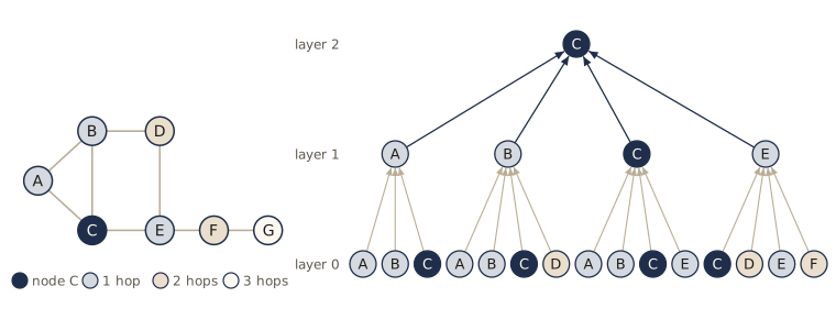
On large, sparse graphs with long distances, a node may need many layers before it hears from the other side of the graph. One fix is to add a virtual node (or super-node) joined to every node: any two nodes are then at most two edges apart, and the virtual node acts as a global summary that every node reads and writes. We will see the same idea again as a graph-level embedding.
What message passing can and cannot distinguish
How much of a graph’s structure can a message-passing network see? There is a clean answer, and it is worth knowing before we train anything.
Consider a classical algorithm for testing whether two graphs might be the same, the Weisfeiler–Lehman test (1-WL, also called color refinement). Give every node the same color. Then, repeatedly, give each node a new color that encodes its current color together with the multiset of its neighbors’ colors (in practice, a lookup table assigns a fresh integer to each distinct combination). Stop when the partition of nodes into colors no longer gets finer. If, at some round, the two graphs have different histograms of colors, they are certainly different (not isomorphic, meaning not equal up to a relabeling). If the histograms stay the same, the test is inconclusive.
Now compare with a message-passing network whose nodes all start with the same feature. At layer \(l\), a node’s embedding is a function of its own embedding and the multiset of its neighbors’ embeddings at layer \(l-1\), the same functions at every node. By induction on \(l\): two nodes with the same WL color after \(l\) rounds have the same embedding after \(l\) layers (their inputs to the layer are equal, so their outputs are). Hence:
Result. If the Weisfeiler–Lehman test cannot distinguish two graphs, then no message-passing network of the kind in this module can either: it assigns the same multiset of node embeddings to both, and therefore the same output to any invariant readout. Conversely, if the aggregation (a sum of transformed neighbor embeddings), the update, and the readout are all injective on their inputs, a message-passing network separates every pair of graphs that the test separates; for node features from a countable set, such functions exist and can be approximated by MLPs (Xu et al., 2019; Morris et al., 2019). With mean or max aggregation, message passing is strictly weaker than the test.
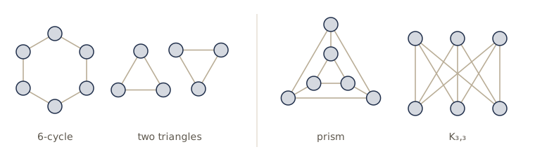
The Graph Isomorphism Network (GIN) of Xu et al. is designed to reach this bound, with the layer \(\mathbf{h}_n^{(l+1)} = \mathrm{MLP}\big( (1 + \epsilon)\mathbf{h}_n^{(l)} + \sum_{m \in \mathcal{N}(n)} \mathbf{h}_m^{(l)} \big)\). The bound itself is real, and simple graphs hit it. Every node of a regular graph (all nodes of equal degree) receives the same multiset of colors in the first round, so the coloring never splits, and any two regular graphs with the same size and degree look identical to the test. We implement the test and check three pairs: a 6-cycle against two separate triangles (both 2-regular), the triangular prism against the complete bipartite graph \(K_{3,3}\) (both 3-regular), and, as a control, a path of four nodes against a star with three leaves. For each pair we also run a randomly initialized sum-aggregation network (three MPLayers with constant input features and a sum readout).
def wl_colors(G, rounds):
    """1-WL color refinement: new color = (own color, sorted neighbor colors), as an integer."""
    colors = {v: 0 for v in G}
    for _ in range(rounds):
        signature = {v: (colors[v], tuple(sorted(colors[u] for u in G[v]))) for v in G}
        table = {s: i for i, s in enumerate(sorted(set(signature.values())))}
        colors = {v: table[signature[v]] for v in G}
    return colors

def wl_same(G1, G2, rounds=5):
    """Run 1-WL on the disjoint union so that colors are comparable, and compare the histograms."""
    U = nx.disjoint_union(G1, G2)
    c, n1 = wl_colors(U, rounds), G1.number_of_nodes()
    hist = lambda nodes: collections.Counter(c[v] for v in nodes)
    return hist(range(n1)) == hist(range(n1, U.number_of_nodes()))

torch.manual_seed(13)
wl_layers = nn.ModuleList([MPLayer(1, 16), MPLayer(16, 16), MPLayer(16, 16)])
def graph_readout(G):
    A_G = torch.tensor(nx.to_numpy_array(G), dtype=torch.float32)
    H = torch.ones(len(A_G), 1)                               # no features: every node starts equal
    for layer in wl_layers:
        H = layer(H, A_G)
    return H.sum(0)

def triangles(G):
    A_G = torch.tensor(nx.to_numpy_array(G), dtype=torch.float32)
    return int(torch.trace(A_G @ A_G @ A_G).item() / 6)

test_pairs = [("6-cycle", nx.cycle_graph(6),
               "two triangles", nx.disjoint_union(nx.cycle_graph(3), nx.cycle_graph(3))),
              ("prism", nx.circular_ladder_graph(3), "K_3,3", nx.complete_bipartite_graph(3, 3)),
              ("path P4", nx.path_graph(4), "star S3", nx.star_graph(3))]
with torch.no_grad():
    for n1, G1, n2, G2 in test_pairs:
        gap = (graph_readout(G1) - graph_readout(G2)).abs().max().item()
        print(f"{n1:8s} vs {n2:13s} isomorphic: {nx.is_isomorphic(G1, G2)!s:5s}"
              f"  WL same: {wl_same(G1, G2)!s:5s}"
              f"  GNN readout gap {gap:.1e}  triangles {triangles(G1)} vs {triangles(G2)}")
6-cycle  vs two triangles isomorphic: False  WL same: True   GNN readout gap 0.0e+00  triangles 0 vs 2
prism    vs K_3,3         isomorphic: False  WL same: True   GNN readout gap 0.0e+00  triangles 2 vs 0
path P4  vs star S3       isomorphic: False  WL same: False  GNN readout gap 1.6e+00  triangles 0 vs 0
The first two pairs are different graphs (one has triangles and the other has none), yet the WL test and the network see them as identical, down to the last bit. The control pair is told apart by both. Counting triangles, detecting cycles of a given length, and many other properties chemists care about are, in general, beyond plain message passing.
There are several standard ways past the limit. One can add features that message passing cannot compute, such as the number of triangles through each node, the node’s degree, or random features that break symmetries; one can pass messages between pairs or triples of nodes instead of single nodes (higher-order networks, matching the stronger \(k\)-WL tests at higher cost); or one can use the node positions available in geometric data, as at the end of this module. The first is a one-line change here: give each node its triangle count, \(\tfrac{1}{2}(\mathbf{A}^3)_{nn}\), as its input feature, and the prism and \(K_{3,3}\) separate at once (exercise 4 asks you to check this).
Update operators
With the aggregation fixed, the update decides how the message is combined with the node’s own state. The linear-plus-nonlinearity form
\[\operatorname{Update}(\mathbf{h}_n, \mathbf{z}_n) = f\big( \mathbf{W}_{\mathrm{self}}\mathbf{h}_n + \mathbf{W}_{\mathrm{neigh}}\mathbf{z}_n + \mathbf{b} \big)\]is the one in MPLayer, and the GCN is the special case with one shared matrix (and the symmetric normalization folded into the aggregation). Common variations replace the linear map with a small MLP (as in GIN), use a gated recurrent unit to combine old state and message, or add the old state back as a residual connection, \(\mathbf{h}_n^{(l+1)} = \mathbf{h}_n^{(l)} + \operatorname{Update}(\cdot)\), which will matter when we make networks deep.
The first layer needs an input embedding \(\mathbf{h}_n^{(0)}\). The observed features \(\mathbf{x}_n\) are the usual choice; to change their dimension we can apply a learnable linear map (or pad with zeros). When nodes have no features at all, a constant vector works, and a one-hot encoding of the node’s degree is a better start, since it gives the first layer something to distinguish.
Stacking layers gives the network
\[\mathbf{H}^{(1)} = F\big(\mathbf{X}, \mathbf{A}, \mathbf{W}^{(1)}\big), \quad \mathbf{H}^{(2)} = F\big(\mathbf{H}^{(1)}, \mathbf{A}, \mathbf{W}^{(2)}\big), \quad \dots, \quad \mathbf{H}^{(L)} = F\big(\mathbf{H}^{(L-1)}, \mathbf{A}, \mathbf{W}^{(L)}\big),\]where \(\mathbf{W}^{(l)}\) stands for all parameters of layer \(l\). Each layer is equivariant, \(F(\mathbf{P}\mathbf{H}, \mathbf{P}\mathbf{A}\mathbf{P}^{\mathrm{T}}, \mathbf{W}) = \mathbf{P}F(\mathbf{H}, \mathbf{A}, \mathbf{W})\), so the stack is too, as we proved and checked above. What remains is the output layer, which depends on the task.
Node classification
For classifying nodes into \(K\) classes, the output layer applies one shared linear map and a softmax at every node,
\[y_{nk} = \frac{\exp\big(\mathbf{w}_k^{\mathrm{T}}\mathbf{h}_n^{(L)}\big)}{\sum_{j=1}^{K} \exp\big(\mathbf{w}_j^{\mathrm{T}}\mathbf{h}_n^{(L)}\big)},\]and the error is the cross-entropy summed over the labeled training nodes \(\mathcal{V}_{\mathrm{train}}\) only,
\[E(\mathbf{w}) = -\sum_{n \in \mathcal{V}_{\mathrm{train}}} \sum_{k=1}^{K} t_{nk} \ln y_{nk},\]with one-hot targets \(t_{nk}\). Since the output weights are shared across nodes, the outputs are equivariant and the error is invariant. (For continuous node targets, use a linear output and a sum-of-squares error.)
Nodes play three roles, and it helps to name them.
- Training nodes \(\mathcal{V}_{\mathrm{train}}\) are labeled; they take part in message passing and in the error.
- Transductive nodes \(\mathcal{V}_{\mathrm{trans}}\) are unlabeled but present during training. They pass messages (so their features and edges shape the embeddings of the training nodes), they do not enter the error, and we predict their labels.
- Inductive nodes \(\mathcal{V}_{\mathrm{induct}}\) are absent during training: neither they nor their edges take part. At prediction time they join the graph and we predict their labels.
Training with transductive nodes is transductive, semi-supervised learning; training without them is inductive.
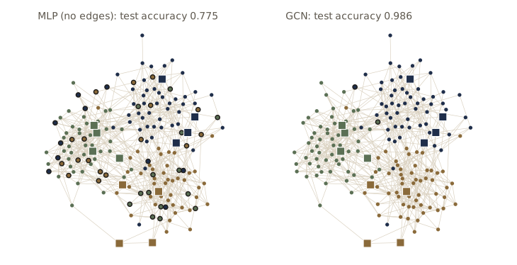
Data. We use a stochastic block model (SBM), the standard random-graph model of communities. The \(N\) nodes are divided into \(K\) blocks; each pair of nodes is joined independently, with probability \(p_{\mathrm{in}}\) if they are in the same block and \(p_{\mathrm{out}}\) otherwise. With \(p_{\mathrm{in}} > p_{\mathrm{out}}\), the graph has communities, and a node’s block is its class. We give each node a 16-dimensional feature vector: the mean vector of its class plus Gaussian noise so large that the features alone are only weakly informative. Only four nodes per class are labeled.
def sbm(sizes, P_blocks, g):
    """Adjacency matrix and block labels of a stochastic block model."""
    labels = np.repeat(np.arange(len(sizes)), sizes)
    probs = np.asarray(P_blocks)[labels][:, labels]
    upper = np.triu(g.random(probs.shape) < probs, k=1)
    return torch.from_numpy((upper | upper.T).astype(np.float32)), torch.from_numpy(labels)

g = np.random.default_rng(1)
K, n_per_block, D = 3, 60, 16
p_in, p_out = 0.10, 0.01
A_sbm, t_sbm = sbm([n_per_block] * K, np.where(np.eye(K) > 0, p_in, p_out), g)
N_sbm = len(t_sbm)
class_means = g.normal(size=(K, D))
X_sbm = torch.from_numpy(class_means[t_sbm.numpy()] + 2.5 * g.normal(size=(N_sbm, D))).float()

deg_sbm = A_sbm.sum(1)
within = (A_sbm * (t_sbm[:, None] == t_sbm[None, :])).sum() / A_sbm.sum()
print(f"{N_sbm} nodes, {A_sbm.sum().item() / 2:.0f} edges, "
      f"mean degree {deg_sbm.mean().item():.1f}, "
      f"isolated nodes {(deg_sbm == 0).sum().item()}, edges inside blocks {within.item():.1%}")

order = g.permutation(N_sbm)
train_idx = torch.from_numpy(np.concatenate(
    [order[t_sbm.numpy()[order] == k][:4] for k in range(K)]))           # 4 per class
rest = np.setdiff1d(order, train_idx.numpy())
rest = torch.from_numpy(rest[g.permutation(len(rest))])
val_idx, test_idx = rest[:30], rest[30:]
print(f"labeled {len(train_idx)}, validation {len(val_idx)}, test {len(test_idx)}")
180 nodes, 614 edges, mean degree 6.8, isolated nodes 0, edges inside blocks 82.6%
labeled 12, validation 30, test 138
Model. A two-layer GCN with dropout, the configuration of Kipf and Welling: \(\mathbf{Y} = \operatorname{softmax}\big(\mathbf{S}\,\mathrm{ReLU}(\mathbf{S}\mathbf{X}\mathbf{W}^{(1)})\mathbf{W}^{(2)}\big)\), with 32 hidden units. The baseline is the same network with \(\mathbf{S}\) replaced by the identity: a graph with no edges, which is an ordinary two-layer MLP applied to each node separately. Everything else, including the optimizer, weight decay, and number of epochs, is the same.
class GCN(nn.Module):
    """Two-layer GCN: S ReLU(S X W1) W2 (logits), with dropout. S = I gives a plain MLP."""
    def __init__(self, d_in, d_hidden, d_out, p_drop=0.5):
        super().__init__()
        self.lin1, self.lin2 = nn.Linear(d_in, d_hidden), nn.Linear(d_hidden, d_out)
        self.p_drop = p_drop
    def forward(self, X, S):
        H = F.dropout(X, self.p_drop, self.training)
        H = torch.relu(S @ self.lin1(H))
        H = F.dropout(H, self.p_drop, self.training)
        return S @ self.lin2(H)

def train_nodes(make_model, X, G, idx, t, epochs=200, lr=0.01, weight_decay=5e-4, seed=0):
    """Full-batch training on the labeled nodes idx; G is whatever the model uses for the graph."""
    torch.manual_seed(seed)
    model = make_model()
    opt = torch.optim.Adam(model.parameters(), lr=lr, weight_decay=weight_decay)
    for epoch in range(epochs):
        model.train()
        loss = F.cross_entropy(model(X, G)[idx], t[idx])
        opt.zero_grad()
        loss.backward()
        opt.step()
    return model

def node_accuracy(model, X, G, idx, t):
    model.eval()
    with torch.no_grad():
        return (model(X, G)[idx].argmax(1) == t[idx]).float().mean().item()

S_sbm = gcn_norm(A_sbm)
I_sbm = torch.eye(N_sbm)
for seed in range(3):
    gcn = train_nodes(lambda: GCN(D, 32, K), X_sbm, S_sbm, train_idx, t_sbm, seed=seed)
    mlp = train_nodes(lambda: GCN(D, 32, K), X_sbm, I_sbm, train_idx, t_sbm, seed=seed)
    print(f"seed {seed}:  GCN test accuracy {node_accuracy(gcn, X_sbm, S_sbm, test_idx, t_sbm):.3f}"
          f"   MLP (no edges) {node_accuracy(mlp, X_sbm, I_sbm, test_idx, t_sbm):.3f}")
seed 0:  GCN test accuracy 0.986   MLP (no edges) 0.775
seed 1:  GCN test accuracy 0.978   MLP (no edges) 0.739
seed 2:  GCN test accuracy 0.978   MLP (no edges) 0.725
With 12 labels and noisy features, the MLP gets about three test nodes in four right. The GCN, which sees the same features but averages them over each node’s neighborhood (most of whose members share the node’s class), gets nearly all of them. The gap would be larger still with noisier features or fewer labels (exercise 6 goes to the extreme of one label per class and no informative features). Two effects combine: averaging reduces the feature noise, and the unlabeled nodes carry the class information of the few labeled ones through the graph.
Inductive use. Because the GCN’s parameters are shared across nodes, a trained model can be applied to nodes it never saw. To test this we remove the test nodes and all their edges, train on the remaining graph, then put them back and predict. The normalization \(\mathbf{S}\) is recomputed for each graph.
seen = torch.from_numpy(np.setdiff1d(np.arange(N_sbm), test_idx.numpy()))  # train + transductive
A_seen = A_sbm[seen][:, seen]
new_index = {int(n): i for i, n in enumerate(seen)}
train_idx_seen = torch.tensor([new_index[int(n)] for n in train_idx])
accs = []
for seed in range(3):
    gcn = train_nodes(lambda: GCN(D, 32, K), X_sbm[seen], gcn_norm(A_seen), train_idx_seen,
                      t_sbm[seen], seed=seed)
    accs.append(node_accuracy(gcn, X_sbm, S_sbm, test_idx, t_sbm))   # full graph at prediction
print("inductive test accuracy, seeds 0-2:", [f"{a:.3f}" for a in accs])
inductive test accuracy, seeds 0-2: ['0.906', '0.935', '0.935']
The accuracy is a few points below the transductive result (about 0.98) but far above the MLP. The test nodes and their edges were never seen in training, so the training graph was smaller and the labeled nodes received less information through it; still, the learned functions transfer to the new nodes, because they are the same functions at every node.
Edge classification
Many graph problems are about pairs of nodes: will these two users connect, does this drug interact with that protein, is this edge in a road network congested? The commonest is link prediction: given a graph with some edges missing, score every non-edge by how likely it is to be a real edge. A GNN solves it in two stages. An encoder (a message-passing network) computes node embeddings \(\mathbf{h}_n\) from the observed graph; a decoder turns a pair of embeddings into a probability. The simplest decoder is the dot product,
\[p(n, m) = \sigma\big( \mathbf{h}_n^{\mathrm{T}}\mathbf{h}_m \big),\]which is symmetric in \(n\) and \(m\), as an undirected edge should be. (For directed edges or several edge types, a bilinear form \(\mathbf{h}_n^{\mathrm{T}}\mathbf{R}_r\mathbf{h}_m\) with a learned matrix per relation type is a common choice.)
Doing this properly involves three details that are easy to get wrong.
- Held-out edges must be removed from the graph the encoder sees. We split the edges into training, validation, and test sets and run message passing on the training edges only. If a test edge stays in the graph, its two nodes exchange messages directly, and the model is partly told the answer.
- Negative examples. The training edges are positive examples. The negatives are non-edges, pairs of nodes that are not linked, and there are far more of them than edges (about \(N^2/2\) against \(E\)). We use negative sampling: at every epoch, draw as many random node pairs as there are training edges and treat them as negatives. A random pair is almost never a true edge in a sparse graph, and drawing fresh pairs every epoch lets the model see many different negatives.
- Evaluation by ranking. At test time we score the held-out edges and an equal number of sampled non-edges. The usual metric is the area under the ROC curve (AUC, see module 05): the probability that a randomly chosen positive gets a higher score than a randomly chosen negative, with ties counted as one half. Computed that way it needs no threshold, and we can do it by comparing all pairs.
Data. An SBM is a poor test bed for link prediction: given the blocks, its edges are independent coin flips, so nothing beyond block membership can be predicted. Real networks have structure beyond communities, in particular triadic closure (friends of friends tend to be friends). A simple model with that property is a latent-space graph: each node has a hidden position in the unit square, nodes closer than a radius \(r\) are joined with high probability, and a few random long-range edges are added. The node features are a noisy linear function of the hidden position, so they carry some information about where the node is, but not much.
def latent_space_graph(N, radius, p_near, p_far, D, noise, g):
    """Hidden positions in the unit square; pairs closer than radius linked with prob. p_near,
    all other pairs with prob. p_far."""
    pos = g.random((N, 2))
    dist = np.sqrt(((pos[:, None] - pos[None]) ** 2).sum(-1))
    upper = np.triu(g.random((N, N)) < np.where(dist < radius, p_near, p_far), k=1)
    A = torch.from_numpy((upper | upper.T).astype(np.float32))
    X = pos @ g.normal(size=(2, D)) + noise * g.normal(size=(N, D))
    return A, torch.from_numpy(X).float(), pos

g = np.random.default_rng(2)
N_lp = 300
A_lp, X_lp, pos_lp = latent_space_graph(N_lp, 0.09, 0.9, 0.004, 16, 1.0, g)
iu = torch.triu_indices(N_lp, N_lp, 1)
all_edges = iu[:, A_lp[iu[0], iu[1]] > 0]                    # each undirected edge once, n < m
E_lp = all_edges.shape[1]
shuffled = all_edges[:, torch.from_numpy(g.permutation(E_lp))]
n_test, n_val = E_lp // 10, E_lp // 20
test_pos, val_pos = shuffled[:, :n_test], shuffled[:, n_test:n_test + n_val]
train_pos = shuffled[:, n_test + n_val:]
A_lp_train = torch.zeros(N_lp, N_lp)
A_lp_train[train_pos[0], train_pos[1]] = 1.0
A_lp_train = A_lp_train + A_lp_train.T              # the graph the encoder is allowed to see

def sample_non_edges(A, k, g):
    """k distinct node pairs (n < m) that are not edges of A."""
    pairs = set()
    while len(pairs) < k:
        n, m = g.integers(len(A), size=2)
        if n != m and A[n, m] == 0:
            pairs.add((min(n, m), max(n, m)))
    return torch.tensor(sorted(pairs)).T

test_neg, val_neg = sample_non_edges(A_lp, n_test, g), sample_non_edges(A_lp, n_val, g)
print(f"{N_lp} nodes, {E_lp} edges, mean degree {A_lp.sum(1).mean().item():.1f}")
print(f"edges: train {train_pos.shape[1]}, validation {n_val}, test {n_test};"
      f"  sampled test non-edges {test_neg.shape[1]}")
300 nodes, 1137 edges, mean degree 7.6
edges: train 968, validation 56, test 113;  sampled test non-edges 113
Next, the AUC. With \(s^{+}_i\) the scores of the \(P\) positive pairs and \(s^{-}_j\) those of the \(Q\) negative ones,
\[\mathrm{AUC} = \frac{1}{PQ}\sum_{i=1}^{P}\sum_{j=1}^{Q} \Big( [s^{+}_i > s^{-}_j] + \tfrac{1}{2}[s^{+}_i = s^{-}_j] \Big),\]where \([\cdot]\) is 1 when the condition holds and 0 otherwise. We check it against the area under the ROC curve computed by sweeping a threshold and integrating with the trapezoid rule, on scores with many ties.
def auc(pos_scores, neg_scores):
    """P(random positive outscores random negative), ties count one half."""
    diff = pos_scores[:, None] - neg_scores[None, :]
    return ((diff > 0).float() + 0.5 * (diff == 0).float()).mean().item()

def roc_curve(pos_scores, neg_scores):
    """False- and true-positive rates for every threshold, from high to low."""
    all_scores = torch.cat([pos_scores, neg_scores]).unique().flip(0)      # high to low
    thresholds = torch.cat([torch.tensor([float("inf")]), all_scores])
    tpr = torch.stack([(pos_scores >= th).float().mean() for th in thresholds])
    fpr = torch.stack([(neg_scores >= th).float().mean() for th in thresholds])
    return fpr, tpr

s_pos = torch.from_numpy(g.integers(0, 6, size=40)).float() + 1.0      # scores with many ties
s_neg = torch.from_numpy(g.integers(0, 6, size=50)).float()
fpr, tpr = roc_curve(s_pos, s_neg)
print(f"pairwise AUC {auc(s_pos, s_neg):.4f}"
      f"   trapezoid area under ROC {torch.trapezoid(tpr, fpr).item():.4f}")
pairwise AUC 0.5200 trapezoid area under ROC 0.5200
Now the model: a two-layer GCN encoder with 64 hidden units and 32-dimensional output embeddings, the dot-product decoder, and the binary cross-entropy on training edges and fresh random pairs. We compare it with the same encoder with no edges (an MLP on the features), with a classical heuristic that needs no learning, the number of common neighbors \((\mathbf{A}^2)_{nm}\) in the training graph, and with a GCN that commits the leakage mistake of running on the full graph, test edges included.
class Encoder(nn.Module):
    """Two GCN layers, no output nonlinearity: node embeddings for the dot-product decoder."""
    def __init__(self, d_in, d_hidden, d_out):
        super().__init__()
        self.lin1, self.lin2 = nn.Linear(d_in, d_hidden), nn.Linear(d_hidden, d_out)
    def forward(self, X, S):
        return S @ self.lin2(torch.relu(S @ self.lin1(X)))

def edge_logits(H, pairs):
    return (H[pairs[0]] * H[pairs[1]]).sum(1)                     # h_n^T h_m

def train_link_predictor(S, epochs=300, seed=0):
    torch.manual_seed(seed)
    g_neg = np.random.default_rng(seed)
    enc = Encoder(X_lp.shape[1], 64, 32)
    opt = torch.optim.Adam(enc.parameters(), lr=0.01)
    n_pos = train_pos.shape[1]
    targets = torch.cat([torch.ones(n_pos), torch.zeros(n_pos)])
    for epoch in range(epochs + 1):
        H = enc(X_lp, S)
        neg = torch.from_numpy(g_neg.integers(N_lp, size=(2, n_pos)))    # fresh random pairs
        loss = F.binary_cross_entropy_with_logits(
            torch.cat([edge_logits(H, train_pos), edge_logits(H, neg)]), targets)
        opt.zero_grad()
        loss.backward()
        opt.step()
    with torch.no_grad():
        H = enc(X_lp, S)
        val = auc(edge_logits(H, val_pos), edge_logits(H, val_neg))
        return edge_logits(H, test_pos), edge_logits(H, test_neg), val

results = {}
for name, S in [("GCN", gcn_norm(A_lp_train)), ("MLP (no edges)", torch.eye(N_lp)),
                ("GCN, test edges leaked", gcn_norm(A_lp))]:
    s_pos, s_neg, val = train_link_predictor(S)
    results[name] = (s_pos, s_neg)
    print(f"{name:24s} validation AUC {val:.3f}   test AUC {auc(s_pos, s_neg):.3f}")
CN = A_lp_train @ A_lp_train
results["common neighbors"] = (CN[test_pos[0], test_pos[1]], CN[test_neg[0], test_neg[1]])
print(f"{'common neighbors':24s} {'':20s} test AUC {auc(*results['common neighbors']):.3f}")
GCN                      validation AUC 0.883   test AUC 0.906
MLP (no edges)           validation AUC 0.741   test AUC 0.826
GCN, test edges leaked   validation AUC 0.944   test AUC 0.962
common neighbors                              test AUC 0.878
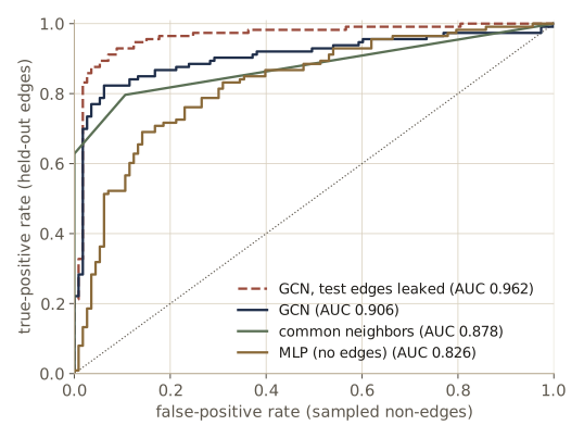
Three lessons. The graph helps: the GCN’s embeddings combine a node’s noisy features with its neighbors’, which locates the node much better, and its AUC is well above the MLP’s. The leaked model looks better still, for the wrong reason, which is why the split must be done before message passing (the validation AUCs, used to choose hyperparameters, must be leak-free too). And the common-neighbors count, a one-line heuristic, is a serious competitor. That last point is not an accident of this data set. A dot product of two node embeddings, each computed separately, cannot in general represent how many neighbors the two nodes share. Link-prediction models that do better on such graphs look at the pair jointly, for example by running message passing on the subgraph around both nodes with the two target nodes marked, or by feeding pairwise features such as the common-neighbor count into the decoder (exercise 7).
Watch out. Random negatives are easy negatives: most random pairs in a spatial or community-structured graph are far apart, and any model that roughly locates nodes will rank them low. An AUC measured against random pairs can therefore look excellent while the model is poor at the question that matters in practice, which is ranking the handful of plausible candidates near a node. Ranking metrics over all candidates of a node (hits at \(k\), mean reciprocal rank), and harder negatives drawn from nearby nodes, give a more honest picture.
Graph classification
For a property of a whole graph we need an invariant output. After the last message-passing layer, a readout combines all node embeddings into one vector and a small network maps it to the prediction:
\[\mathbf{y} = f\Big( \sum_{n \in \mathcal{V}} \mathbf{h}_n^{(L)} \Big).\]The sum is invariant because it is a sum; the mean and the element-wise max are the usual alternatives (the mean when graph sizes vary a lot and size itself should not matter). The training set is now a set of graphs \(G_1, \dots, G_N\) with labels, and the task is inductive: test graphs are new graphs. Cross-entropy is the usual error for classification (a molecule is toxic or not), sum-of-squares for regression (its solubility).
Batching. Graphs in a data set have different sizes, so we cannot stack them into one tensor. The standard trick is to put a mini-batch of graphs into one big graph with no edges between the pieces. Its adjacency matrix is block diagonal, with one block per graph, so messages never cross from one graph to another. In edge-list form we simply concatenate the edge lists, shifting the node numbers of each graph by the number of nodes before it, and keep a batch vector that records which graph each node belongs to. The readout is then a scatter-add of node embeddings into their graph’s row.
Data. We make a data set of 600 graphs with 12 to 24 nodes. Half are random geometric graphs: nodes at random points in the unit square, joined when closer than 0.3. The other half are random graphs with exactly the same number of nodes and edges, the edges placed uniformly at random (Erdős–Rényi graphs conditioned on the edge count). Each geometric graph is paired with a random one of the same size and density, so counting nodes or edges is useless. What separates them is local structure: in a geometric graph, two neighbors of a node are likely to be close to each other and therefore linked, so there are many triangles. Nodes have no features; we use the one-hot degree (capped at 10) as input, as suggested above.
def geometric_graph(n, radius, g):
    pts = g.random((n, 2))
    close = ((pts[:, None] - pts[None]) ** 2).sum(-1) < radius ** 2
    np.fill_diagonal(close, False)
    return close.astype(np.float32)

def random_graph_like(A, g):
    """Uniformly random graph with the same number of nodes and edges as A."""
    n = len(A)
    iu = np.triu_indices(n, 1)
    pick = g.choice(len(iu[0]), int(A.sum() / 2), replace=False)
    B = np.zeros((n, n), np.float32)
    B[iu[0][pick], iu[1][pick]] = 1.0
    return B + B.T

g = np.random.default_rng(3)
graphs, labels = [], []
for i in range(300):
    A_geo = geometric_graph(int(g.integers(12, 25)), 0.3, g)
    graphs += [A_geo, random_graph_like(A_geo, g)]
    labels += [1, 0]
y_graphs = torch.tensor(labels)
tri = np.array([np.trace(G @ G @ G) / 6 for G in graphs])
print(f"{len(graphs)} graphs, {np.mean([len(G) for G in graphs]):.1f} nodes and "
      f"{np.mean([G.sum() / 2 for G in graphs]):.1f} edges on average")
print(f"mean number of triangles: geometric {tri[y_graphs == 1].mean():.1f},"
      f" random {tri[y_graphs == 0].mean():.1f}")

MAX_DEG = 10
def batch_graphs(adjs):
    """Many graphs as one block-diagonal graph: edge list, one-hot degree features, batch vector."""
    edges, feats, batch, offset = [], [], [], 0
    for gi, Ag in enumerate(adjs):
        edges.append(np.stack(np.nonzero(Ag)) + offset)
        degree = np.minimum(Ag.sum(1).astype(int), MAX_DEG)
        feats.append(np.eye(MAX_DEG + 1, dtype=np.float32)[degree])
        batch.append(np.full(len(Ag), gi))
        offset += len(Ag)
    return (torch.from_numpy(np.concatenate(feats)),
            torch.from_numpy(np.concatenate(edges, 1)).long(),
            torch.from_numpy(np.concatenate(batch)).long())

X_b, ei_b, batch_b = batch_graphs(graphs[:3])
print("three graphs as one:", tuple(X_b.shape), "node features,", ei_b.shape[1], "directed edges,",
      "batch vector counts", torch.bincount(batch_b).tolist())
600 graphs, 17.9 nodes and 33.8 edges on average
mean number of triangles: geometric 29.2, random 9.6
three graphs as one: (64, 11) node features, 292 directed edges, batch vector counts [22, 22, 20]
The model is a GIN-style network: an input linear map, then \(L\) layers of sum aggregation with a two-layer MLP as the update, \(\mathbf{h}_n \leftarrow \mathrm{MLP}\big(\mathbf{h}_n + \sum_{m \in \mathcal{N}(n)} \mathbf{h}_m\big)\), then a sum readout and a small MLP classifier. Before training, we check that batching changes nothing: the output for a batch of three graphs must equal the outputs for the three graphs run one at a time.
class GIN(nn.Module):
    def __init__(self, d_in, d_hidden, n_layers, n_classes):
        super().__init__()
        self.embed = nn.Linear(d_in, d_hidden)
        self.updates = nn.ModuleList([
            nn.Sequential(nn.Linear(d_hidden, d_hidden), nn.ReLU(),
                          nn.Linear(d_hidden, d_hidden), nn.ReLU())
            for _ in range(n_layers)])
        self.classify = nn.Sequential(nn.Linear(d_hidden, d_hidden), nn.ReLU(),
                                      nn.Linear(d_hidden, n_classes))
    def forward(self, X, edge_index, batch, n_graphs):
        H = self.embed(X)
        for update in self.updates:
            H = update(H + aggregate_sum(H, edge_index))
        readout = torch.zeros(n_graphs, H.shape[1]).index_add_(0, batch, H)    # sum per graph
        return self.classify(readout)

torch.manual_seed(13)
gin = GIN(MAX_DEG + 1, 32, 2, 2)
with torch.no_grad():
    together = gin(X_b, ei_b, batch_b, 3)
    one_by_one = torch.cat([gin(*batch_graphs([G]), 1) for G in graphs[:3]])
print(f"batched vs one graph at a time: {(together - one_by_one).abs().max().item():.1e}")
batched vs one graph at a time: 6.0e-07
We train with mini-batches of 50 graphs for 60 epochs, for networks with 0 to 3 message-passing layers. With zero layers the readout is the sum of the input features, which is just the histogram of degrees: a baseline that sees the degree distribution and nothing else.
train_ids, test_ids = np.arange(400), np.arange(400, 600)
full_train = batch_graphs([graphs[i] for i in train_ids])
full_test = batch_graphs([graphs[i] for i in test_ids])

def graph_accuracy(model, batched, ids):
    X_, ei_, b_ = batched
    with torch.no_grad():
        return (model(X_, ei_, b_, len(ids)).argmax(1) == y_graphs[ids]).float().mean().item()

for n_layers in [0, 1, 2, 3]:
    torch.manual_seed(0)
    g_batches = np.random.default_rng(0)
    model = GIN(MAX_DEG + 1, 32, n_layers, 2)
    opt = torch.optim.Adam(model.parameters(), lr=0.005)
    for epoch in range(60):
        shuffle = g_batches.permutation(train_ids)
        for start in range(0, len(shuffle), 50):
            ids = shuffle[start:start + 50]
            X_, ei_, b_ = batch_graphs([graphs[i] for i in ids])
            loss = F.cross_entropy(model(X_, ei_, b_, len(ids)), y_graphs[ids])
            opt.zero_grad()
            loss.backward()
            opt.step()
    print(f"{n_layers} message-passing layers:"
          f"  train accuracy {graph_accuracy(model, full_train, train_ids):.3f}"
          f"   test accuracy {graph_accuracy(model, full_test, test_ids):.3f}")
0 message-passing layers:  train accuracy 0.780   test accuracy 0.575
1 message-passing layers:  train accuracy 0.930   test accuracy 0.895
2 message-passing layers:  train accuracy 0.962   test accuracy 0.890
3 message-passing layers:  train accuracy 0.965   test accuracy 0.895
The degree histogram alone is barely better than chance on the test set, and what it learns on the training set does not transfer. One layer of message passing makes a large difference: a node now knows the degrees of its neighbors, and in a geometric graph, where dense regions and sparse regions are spatially coherent, neighbors of high-degree nodes tend to have high degree too. More layers help little here. Recall from the WL discussion that no amount of message passing counts triangles exactly; the network separates the classes through correlated, WL-visible statistics. A GPU, more graphs, and tuning (the hidden size, a validation set for early stopping) would push the accuracy higher.
General graph networks
The layers so far keep one vector per node. This section extends them in three directions (attention over neighbors, vectors on edges, and a vector for the whole graph), then turns to the two practical problems of deep graph networks, over-smoothing and regularization, and ends with networks that respect the geometry of points in space.
Graph attention networks
Sum and mean aggregation weight all neighbors equally (or by a fixed function of the degrees). Often some neighbors matter more than others, and which ones depends on the data. Attention, the mechanism of module 12, lets the network decide. The aggregation becomes a weighted average,
\[\mathbf{z}_n = \sum_{m \in \mathcal{N}(n)} A_{nm}\, \mathbf{h}_m, \qquad A_{nm} \ge 0, \qquad \sum_{m \in \mathcal{N}(n)} A_{nm} = 1,\]where the attention coefficients \(A_{nm}\) (not the adjacency matrix; the book uses the same letter) come from a softmax over each neighborhood of a learned score \(e_{nm}\):
\[A_{nm} = \frac{\exp(e_{nm})}{\sum_{m' \in \mathcal{N}(n)} \exp(e_{nm'})}.\]Two choices of score are common. A bilinear form, \(e_{nm} = \mathbf{h}_n^{\mathrm{T}}\mathbf{W}\mathbf{h}_m\), is the transformer’s query–key product with \(\mathbf{W} = \mathbf{W}_q\mathbf{W}_k^{\mathrm{T}}/\sqrt{d}\). The original graph attention network (GAT; Veličković et al., 2018) uses a small learned function of the two transformed embeddings,
\[e_{nm} = \mathrm{LeakyReLU}\big( \mathbf{a}_{\mathrm{dst}}^{\mathrm{T}}\mathbf{W}\mathbf{h}_n + \mathbf{a}_{\mathrm{src}}^{\mathrm{T}}\mathbf{W}\mathbf{h}_m \big),\]aggregates the transformed embeddings \(\mathbf{W}\mathbf{h}_m\), and includes the node itself in its neighborhood (a self-loop). Any score works as long as the same function is used on every edge: the coefficients then depend only on the embeddings at the two ends, so relabeling the nodes relabels the coefficients along with everything else, and the layer stays equivariant. As in a transformer, several heads with separate parameters run in parallel and their outputs are concatenated (or averaged in the last layer).
On an edge list, the softmax runs over the edges that share a target node, a scatter softmax: subtract each target’s maximum score for numerical stability (a scatter-max), exponentiate, and divide by each target’s sum (a scatter-add). We implement a multi-head GAT layer that way and check it three ways: against a dense implementation that masks the non-edges with \(-\infty\) before a row-wise softmax; with the score vectors set to zero, when every score is equal and attention must reduce to a plain mean over the node and its neighbors, \(\hat{\mathbf{D}}^{-1}\hat{\mathbf{A}}\mathbf{H}\mathbf{W}^{\mathrm{T}}\); and, for bilinear scores on a complete graph, against PyTorch’s scaled_dot_product_attention, the transformer’s attention.
def scatter_softmax(e, dst, N):
    """Softmax of edge scores e over the edges that share a target node."""
    e_max = torch.full((N,), -float("inf")).scatter_reduce(0, dst, e, "amax")
    w = torch.exp(e - e_max[dst])
    return w / torch.zeros(N).index_add_(0, dst, w)[dst]

class GATLayer(nn.Module):
    def __init__(self, d_in, d_out, heads=1):
        super().__init__()
        self.W = nn.Linear(d_in, heads * d_out, bias=False)
        self.a_src = nn.Parameter(0.1 * torch.randn(heads, d_out))
        self.a_dst = nn.Parameter(0.1 * torch.randn(heads, d_out))
        self.heads, self.d_out = heads, d_out
    def forward(self, H, edge_index):                        # edge_index must include self-loops
        src, dst = edge_index
        N = H.shape[0]
        WH = self.W(H).view(N, self.heads, self.d_out)
        e = F.leaky_relu((WH[dst] * self.a_dst).sum(-1) + (WH[src] * self.a_src).sum(-1), 0.2)
        self.alpha = torch.stack([scatter_softmax(e[:, k], dst, N) for k in range(self.heads)], 1)
        messages = self.alpha[..., None] * WH[src]                  # A_nm W h_m, per head
        out = torch.zeros(N, self.heads, self.d_out).index_add_(0, dst, messages)
        return out.reshape(N, self.heads * self.d_out)                           # concatenate heads

def with_self_loops(edge_index, N):
    loops = torch.arange(N)
    return torch.cat([edge_index, torch.stack([loops, loops])], 1)

ei_sbm = with_self_loops(A_sbm.nonzero().T, N_sbm)
A_hat_sbm = A_sbm + torch.eye(N_sbm)
torch.manual_seed(13)
gat = GATLayer(D, 8)
with torch.no_grad():
    WH = gat.W(X_sbm)
    e_dense = F.leaky_relu((WH @ gat.a_dst[0])[:, None] + (WH @ gat.a_src[0])[None, :], 0.2)
    att_dense = torch.softmax(e_dense.masked_fill(A_hat_sbm == 0, -float("inf")), dim=1)
    gap = (gat(X_sbm, ei_sbm) - att_dense @ WH).abs().max().item()
    print(f"edge-list GAT vs dense masked softmax: {gap:.1e}")
    gat.a_src.zero_()
    gat.a_dst.zero_()
    mean_agg = (A_hat_sbm / A_hat_sbm.sum(1, keepdim=True)) @ WH
    gap = (gat(X_sbm, ei_sbm) - mean_agg).abs().max().item()
    print(f"equal scores vs mean aggregation:      {gap:.1e}")

    d_k = 8
    W_q, W_k, W_v = (torch.randn(D, d_k) / math.sqrt(D) for _ in range(3))
    Q, K_, V_ = X_sbm @ W_q, X_sbm @ W_k, X_sbm @ W_v
    ours = torch.softmax(Q @ K_.T / math.sqrt(d_k), dim=1) @ V_     # every node attends to all
    library = F.scaled_dot_product_attention(Q[None], K_[None], V_[None])[0]
    print(f"complete-graph attention vs scaled_dot_product_attention: "
          f"{(ours - library).abs().max().item():.1e}"
          f"   (values of size {ours.abs().max().item():.0f})")
edge-list GAT vs dense masked softmax: 3.6e-07
equal scores vs mean aggregation:      2.4e-07
complete-graph attention vs scaled_dot_product_attention: 1.3e-05   (values of size 10)
The last check makes a point worth stating plainly. A transformer layer’s attention is graph attention on the complete graph, where every token is a neighbor of every other token, with bilinear scores; the positional encodings of module 12 are how a transformer puts back the order information that the complete graph does not have. Conversely, a graph attention network is attention masked by the graph’s edges. On a complete graph, a multi-head graph attention layer with bilinear scores, followed by a residual connection, layer normalization, and a feed-forward network on each node, is exactly a transformer encoder layer.
Let us train a two-layer GAT (4 heads of 8 units, then one head for the classes) on the block-model node classification, and look at what it attends to. For each edge we compare the learned coefficient with the uniform value \(1/\hat{d}_n\) that mean aggregation would use.
class GAT(nn.Module):
    def __init__(self, d_in, n_classes, heads=4, d_head=8):
        super().__init__()
        self.layer1 = GATLayer(d_in, d_head, heads)
        self.layer2 = GATLayer(heads * d_head, n_classes, 1)
    def forward(self, X, edge_index):
        H = F.elu(self.layer1(F.dropout(X, 0.5, self.training), edge_index))
        return self.layer2(F.dropout(H, 0.5, self.training), edge_index)

for seed in range(3):
    model = train_nodes(lambda: GAT(D, K), X_sbm, ei_sbm, train_idx, t_sbm, seed=seed)
    acc = node_accuracy(model, X_sbm, ei_sbm, test_idx, t_sbm)
    print(f"seed {seed}: GAT test accuracy {acc:.3f}")

src, dst = ei_sbm
same_block = (t_sbm[src] == t_sbm[dst]) & (src != dst)
other_block = t_sbm[src] != t_sbm[dst]
uniform = 1.0 / A_hat_sbm.sum(1)[dst]
for name, layer in [("layer 1", model.layer1), ("layer 2", model.layer2)]:
    ratio = layer.alpha.mean(1) / uniform
    print(f"{name}: attention / uniform, same-block edges {ratio[same_block].mean().item():.3f},"
          f" other-block edges {ratio[other_block].mean().item():.3f}")
seed 0: GAT test accuracy 0.986
seed 1: GAT test accuracy 0.978
seed 2: GAT test accuracy 0.993
layer 1: attention / uniform, same-block edges 0.990, other-block edges 1.013
layer 2: attention / uniform, same-block edges 1.003, other-block edges 0.985
The GAT does about as well as the GCN here, and its attention hardly departs from uniform: it has not learned to trust same-block neighbors more. Part of the reason is the data: in a block model all same-block neighbors are equally informative, so there is little to gain from weighting them. Part is a known limitation of the GAT score. The softmax over \(m\) is unchanged if we add a constant to all \(e_{nm}\), and since the LeakyReLU is increasing, the order of the scores over \(m\) is set by \(\mathbf{a}_{\mathrm{src}}^{\mathrm{T}}\mathbf{W}\mathbf{h}_m\) alone, the same for every receiving node \(n\). Every node ranks the candidate neighbors in the same order. A node in block 1 cannot prefer block-1 neighbors while a node in block 2 prefers block-2 neighbors, which is exactly what this task would need. Brody, Alon, and Yahav (2022) call this static attention and fix it (GATv2) by applying the nonlinearity before the dot product with \(\mathbf{a}\); the bilinear score also avoids it. Exercise 8 asks you to try both.
Edge embeddings
So far edges only carry messages. In many problems edges have their own data (bond types, distances, road lengths), and even when they do not, it can help to keep a learned vector on every edge. We add an edge embedding \(\mathbf{e}_{nm}^{(l)}\) to each edge and split a layer into three steps:
\[\begin{aligned} \mathbf{e}_{nm}^{(l+1)} &= \operatorname{Update}_{\mathrm{edge}}\big( \mathbf{e}_{nm}^{(l)}, \mathbf{h}_n^{(l)}, \mathbf{h}_m^{(l)} \big), \\ \mathbf{z}_n^{(l+1)} &= \operatorname{Aggregate}_{\mathrm{node}}\big( \{\mathbf{e}_{nm}^{(l+1)} : m \in \mathcal{N}(n)\} \big), \\ \mathbf{h}_n^{(l+1)} &= \operatorname{Update}_{\mathrm{node}}\big( \mathbf{h}_n^{(l)}, \mathbf{z}_n^{(l+1)} \big). \end{aligned}\]The updated edge embedding is now the message: a function of the edge’s own state and the two nodes it joins. The final edge embeddings \(\mathbf{e}_{nm}^{(L)}\) can feed an edge classifier directly (is this bond reactive, is this transaction fraudulent). For an undirected graph stored in both directions, the two copies of an edge get separate embeddings unless we tie them; that is usually harmless.
Graph embeddings
Finally, add one vector \(\mathbf{g}^{(l)}\) for the whole graph, which every edge and node update can read and which is itself updated from all nodes and edges. This is the general graph network block of Battaglia et al. (2018):
\[\begin{aligned} \mathbf{e}_{nm}^{(l+1)} &= \operatorname{Update}_{\mathrm{edge}}\big( \mathbf{e}_{nm}^{(l)}, \mathbf{h}_n^{(l)}, \mathbf{h}_m^{(l)}, \mathbf{g}^{(l)} \big), \\ \mathbf{z}_n^{(l+1)} &= \operatorname{Aggregate}_{\mathrm{node}}\big( \{\mathbf{e}_{nm}^{(l+1)} : m \in \mathcal{N}(n)\} \big), \\ \mathbf{h}_n^{(l+1)} &= \operatorname{Update}_{\mathrm{node}}\big( \mathbf{h}_n^{(l)}, \mathbf{z}_n^{(l+1)}, \mathbf{g}^{(l)} \big), \\ \mathbf{g}^{(l+1)} &= \operatorname{Update}_{\mathrm{graph}}\big( \mathbf{g}^{(l)}, \{\mathbf{h}_n^{(l+1)} : n \in \mathcal{V}\}, \{\mathbf{e}_{nm}^{(l+1)} : (n, m) \in \mathcal{E}\} \big). \end{aligned}\]The order is edges, then nodes, then the graph, each step using the freshest values available. The graph update must be invariant in its sets of nodes and edges, so it aggregates them (sums or means) before combining. The global vector plays the role of the virtual node: it gives every node a summary of the whole graph in a single layer. The block contains everything so far as special cases: drop \(\mathbf{g}\) and the edge states and let the edge update return \(\mathbf{W}\mathbf{h}_m\), and we are back to the GCN family.
We implement one such block with small MLPs for the three updates and sum aggregations, and check its symmetries. Relabeling the nodes with \(\mathbf{P}\) must permute the node outputs, leave the edge outputs attached to the same edges (we keep the edge list in the same order, with the endpoint numbers mapped to the new labels), and leave the graph vector unchanged.
def mlp(d_in, d_out, d_hidden=32):
    return nn.Sequential(nn.Linear(d_in, d_hidden), nn.ReLU(), nn.Linear(d_hidden, d_out))

class GraphNetBlock(nn.Module):
    """Edge, node, and graph updates in the order edges -> nodes -> graph, with sum aggregations."""
    def __init__(self, d_node, d_edge, d_graph):
        super().__init__()
        self.edge_update = mlp(d_edge + 2 * d_node + d_graph, d_edge)
        self.node_update = mlp(d_node + d_edge + d_graph, d_node)
        self.graph_update = mlp(d_graph + d_node + d_edge, d_graph)
    def forward(self, H, E_feat, g_vec, edge_index):
        src, dst = edge_index                              # edge (m -> n): m = src, n = dst
        n_edges = src.shape[0]
        E_new = self.edge_update(torch.cat([E_feat, H[dst], H[src], g_vec.expand(n_edges, -1)], 1))
        Z = torch.zeros(H.shape[0], E_new.shape[1]).index_add_(0, dst, E_new)
        H_new = self.node_update(torch.cat([H, Z, g_vec.expand(H.shape[0], -1)], 1))
        pooled = torch.cat([H_new.sum(0, keepdim=True), E_new.sum(0, keepdim=True)], 1)
        g_new = self.graph_update(torch.cat([g_vec, pooled], 1))
        return H_new, E_new, g_new

torch.manual_seed(13)
block = GraphNetBlock(d_node=3, d_edge=4, d_graph=2)
E0 = torch.from_numpy(rng.normal(size=(edge_index.shape[1], 4))).float()  # one per directed edge
g0 = torch.zeros(1, 2)
new_label = torch.argsort(perm)              # old node i is called new_label[i] after relabeling
with torch.no_grad():
    H1, E1, g1 = block(X, E0, g0, edge_index)
    H1_t, E1_t, g1_t = block(P @ X, E0, g0, new_label[edge_index])
    print(f"nodes permuted:   {(H1_t - P @ H1).abs().max().item():.1e}")
    print(f"edges unchanged:  {(E1_t - E1).abs().max().item():.1e}")
    print(f"graph invariant:  {(g1_t - g1).abs().max().item():.1e}")
nodes permuted:   3.0e-08
edges unchanged:  0.0e+00
graph invariant:  0.0e+00
Over-smoothing
Convolutional networks for images work best with many layers. Graph networks usually do not: two or three layers are typical, and plain GCNs get worse, not better, as they get deeper. The main reason is over-smoothing: as layers are added, the node embeddings become more and more alike, until they carry almost no information about which node they belong to.
We have already seen why. Without the weights and nonlinearities, \(L\) GCN layers compute \(\mathbf{S}^L\mathbf{X}\). Write \(\mathbf{S} = \sum_i \lambda_i \mathbf{u}_i\mathbf{u}_i^{\mathrm{T}}\) with eigenvalues \(1 = \lambda_1 > \lambda_2 \ge \dots \ge \lambda_N > -1\) (for a connected graph with self-loops the eigenvalue 1 is simple and \(-1\) does not occur). Then
\[\mathbf{S}^L\mathbf{X} = \sum_i \lambda_i^L\, \mathbf{u}_i\mathbf{u}_i^{\mathrm{T}}\mathbf{X} \;\longrightarrow\; \mathbf{u}_1\mathbf{u}_1^{\mathrm{T}}\mathbf{X} \quad \text{as } L \to \infty,\]with \(\mathbf{u}_1 \propto \hat{\mathbf{D}}^{1/2}\mathbf{1}\). In the limit, every node’s embedding is the same vector \(\mathbf{u}_1^{\mathrm{T}}\mathbf{X}\) scaled by \(\sqrt{\hat{d}_n}\): the features have been averaged over the whole graph, and all that remains of a node is its degree. The other components die out like \(\lambda_i^L\), the slowest like \(\lambda_2^L\).
To measure how far this has gone, use the Dirichlet energy from earlier, applied to each column of \(\mathbf{H}\) and normalized by the size of \(\mathbf{H}\) so that shrinking all embeddings does not count as smoothing:
\[R(\mathbf{H}) = \frac{\operatorname{tr}\big(\mathbf{H}^{\mathrm{T}}\hat{\mathbf{L}}\mathbf{H}\big)}{\operatorname{tr}\big(\mathbf{H}^{\mathrm{T}}\mathbf{H}\big)} = \frac{\frac{1}{2}\sum_{n,m} \hat{A}_{nm} \big\lVert \mathbf{h}_n/\sqrt{\hat{d}_n} - \mathbf{h}_m/\sqrt{\hat{d}_m} \big\rVert^2}{\sum_n \lVert \mathbf{h}_n \rVert^2}.\]It lies between 0 (all embeddings proportional to \(\sqrt{\hat{d}_n}\) times a common vector, fully smoothed) and the largest eigenvalue of \(\hat{\mathbf{L}}\) (less than 2). For \(\mathbf{S}^L\mathbf{X}\), it decays roughly like \(\lambda_2^{2L}\) once the other components are gone. We measure it on the block-model graph.
L_hat = torch.eye(N_sbm) - S_sbm
def dirichlet_ratio(H):
    """Normalized Dirichlet energy tr(H^T L H) / tr(H^T H): 0 means fully smoothed."""
    return (torch.trace(H.T @ L_hat @ H) / (H ** 2).sum()).item()

mu = torch.linalg.eigvalsh(L_hat)
lam2 = 1 - mu[1].item()
print(f"second eigenvalue of S: {lam2:.4f}"
      f"  -> energy should shrink by about {lam2 ** 2:.3f} per layer")
H = X_sbm.clone()
for k in range(33):
    if k in (0, 1, 2, 4, 8, 16, 32):
        print(f"S^{k:<2d} X:  R = {dirichlet_ratio(H):.2e}")
    H = S_sbm @ H
second eigenvalue of S: 0.8623  -> energy should shrink by about 0.744 per layer
S^0  X:  R = 7.66e-01
S^1  X:  R = 3.70e-01
S^2  X:  R = 1.88e-01
S^4  X:  R = 8.26e-02
S^8  X:  R = 2.62e-02
S^16 X:  R = 2.20e-03
S^32 X:  R = 1.52e-05
With learned weights and ReLUs between the propagations the picture is similar, and the fix suggested by module 09 is a residual connection, \(\mathbf{H}^{(l+1)} = \mathbf{H}^{(l)} + \mathrm{ReLU}\big(\mathbf{S}\mathbf{H}^{(l)}\mathbf{W}^{(l)}\big)\), which lets each layer add a correction to its input instead of replacing it. A second remedy, sometimes called jumping knowledge, lets the output layer read every layer rather than only the last:
\[\mathbf{y}_n = f\big( \mathbf{h}_n^{(1)} \oplus \mathbf{h}_n^{(2)} \oplus \dots \oplus \mathbf{h}_n^{(L)} \big),\]where \(\oplus\) is concatenation (an element-wise max over the layers is a cheaper variant). The early layers, which are not yet smoothed, then stay available however deep the network is. We build one class with all three variants, first measure the energy through 64 randomly initialized layers, then train networks of increasing depth on the block-model task.
class DeepGCN(nn.Module):
    """L GCN layers of width 32; mode 'plain', 'residual' (layers 2..L), or 'jk' (concatenate)."""
    def __init__(self, d_in, n_classes, n_layers, mode="plain", d_hidden=32):
        super().__init__()
        self.lins = nn.ModuleList([nn.Linear(d_in if l == 0 else d_hidden, d_hidden)
                                   for l in range(n_layers)])
        self.out = nn.Linear(d_hidden * (n_layers if mode == "jk" else 1), n_classes)
        self.mode = mode
    def forward(self, X, S):
        H, layers_out, self.energy = F.dropout(X, 0.5, self.training), [], []
        for l, lin in enumerate(self.lins):
            H_new = torch.relu(S @ lin(H))
            H = H + H_new if (self.mode == "residual" and l > 0) else H_new
            layers_out.append(H)
            if not self.training:
                self.energy.append(dirichlet_ratio(H))
        return self.out(torch.cat(layers_out, 1) if self.mode == "jk" else H)

for mode in ["plain", "residual"]:
    torch.manual_seed(0)
    net = DeepGCN(D, K, 64, mode).eval()
    with torch.no_grad():
        net(X_sbm, S_sbm)
    print(f"random {mode:8s} R after layers 1, 2, 4, 8, 16, 32, 64:",
          " ".join(f"{net.energy[l - 1]:.1e}" for l in (1, 2, 4, 8, 16, 32, 64)))

t_start = time.time()
print("test accuracy     plain  residual  jumping knowledge")
for n_layers in [2, 4, 8, 16, 32]:
    accs = [node_accuracy(train_nodes(lambda: DeepGCN(D, K, n_layers, mode), X_sbm, S_sbm,
                                      train_idx, t_sbm, epochs=150), X_sbm, S_sbm, test_idx, t_sbm)
            for mode in ["plain", "residual", "jk"]]
    print(f"{n_layers:2d} layers         " + "   ".join(f"{a:.3f}" for a in accs))
print(f"(training time, your times will differ: {time.time() - t_start:.0f} s)")
random plain    R after layers 1, 2, 4, 8, 16, 32, 64: 3.0e-01 7.0e-02 3.6e-03 2.0e-03 2.2e-03 1.4e-03 1.9e-03
random residual R after layers 1, 2, 4, 8, 16, 32, 64: 3.0e-01 2.2e-01 1.4e-01 3.6e-02 4.2e-03 1.0e-03 1.4e-04
test accuracy     plain  residual  jumping knowledge
 2 layers         0.964   0.964   0.971
 4 layers         0.957   0.978   0.971
 8 layers         0.826   0.949   0.986
16 layers         0.355   0.942   0.949
32 layers         0.326   0.942   0.978
(training time, your times will differ: 14 s)
The linear propagation and the random plain network both lose most of their energy within a handful of layers; the plain network then levels off near \(2 \times 10^{-3}\) (the input features have 0.77) instead of decaying further. The residual network holds its energy much longer, though by 32 and more random layers it smooths too: the residual sum keeps accumulating smoothed corrections that eventually dominate. Training tells the same story. The plain GCN does well at two and four layers, starts to fail at eight, and is at chance (about 0.33 for three classes) by sixteen; with residual connections or jumping knowledge, deep networks still train and classify well. The best deep networks only match the two-layer ones, to within a few test nodes, which is typical: on graphs where the useful information is within two or three hops, depth mostly adds ways to fail. Depth pays off when long-range information matters, and then remedies like these are needed.
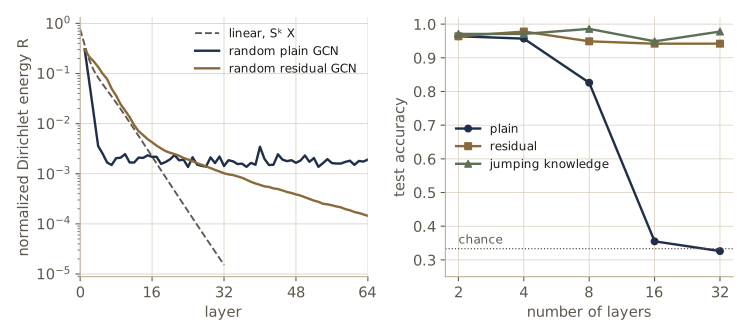
Note. Over-smoothing is not the only obstacle to depth. In a graph whose neighborhoods grow fast, information from an exponentially growing number of nodes must pass through a fixed-size vector at each node, a bottleneck called over-squashing. Adding shortcut edges or a virtual node, or using attention over the whole graph (a graph transformer), are common responses.
Regularization
Graph networks overfit like any network, especially in the transductive setting with a handful of labels. The standard tools of module 09 all apply: weight decay (the weight_decay=5e-4 in our training runs is one), early stopping on validation nodes, and dropout on the features (also in our GCN). Parameters can also be shared across layers, which turns a stack of \(L\) layers into one layer applied \(L\) times and cuts the parameter count by a factor \(L\).
Two regularizers are specific to graphs. Node dropout removes a random subset of nodes, with their edges, at every forward pass during training. DropEdge (Rong et al., 2020) removes a random subset of edges instead: each undirected edge is kept with probability \(1 - p\), independently at every forward pass, and the normalization is recomputed for the thinned graph. Like ordinary dropout it trains the network not to rely on any particular connection; it also slows over-smoothing, since fewer edges mean less mixing per layer. At test time the full graph is used.
def drop_edge(A, p, generator):
    """Remove each undirected edge with probability p (both directions together)."""
    keep = torch.rand(A.shape, generator=generator) >= p
    keep = torch.triu(keep, diagonal=1)
    return A * (keep | keep.T).float()

class DropEdgeGCN(GCN):
    def __init__(self, *args, p_edge=0.3, seed=0):
        super().__init__(*args)
        self.p_edge, self.gen = p_edge, torch.Generator().manual_seed(seed)
    def forward(self, X, A):                    # takes the adjacency matrix, not S
        if self.training:
            A = drop_edge(A, self.p_edge, self.gen)
        return super().forward(X, gcn_norm(A))

thinned = drop_edge(A_sbm, 0.3, torch.Generator().manual_seed(0))
print(f"edges kept in one sample: {thinned.sum().item() / A_sbm.sum().item():.3f},"
      f" still symmetric: {torch.equal(thinned, thinned.T)}")
for seed in range(3):
    model = train_nodes(lambda: DropEdgeGCN(D, 32, K, seed=seed), X_sbm, A_sbm, train_idx, t_sbm,
                        seed=seed)
    acc = node_accuracy(model, X_sbm, A_sbm, test_idx, t_sbm)
    print(f"seed {seed}: GCN with DropEdge, test accuracy {acc:.3f}")
edges kept in one sample: 0.715, still symmetric: True
seed 0: GCN with DropEdge, test accuracy 0.978
seed 1: GCN with DropEdge, test accuracy 0.971
seed 2: GCN with DropEdge, test accuracy 0.971
On this small, easy problem DropEdge makes no useful difference (each seed gets one test node fewer than the plain two-layer GCN); its reported benefits are for deeper networks and larger graphs. Exercise 9 asks you to test it on the deep plain GCN that collapsed above.
Geometric deep learning
Many graphs live in space. A molecule is a set of atoms with three-dimensional coordinates; a mesh in computer graphics is a set of points on a surface; a particle simulation tracks positions and velocities. In these problems the node relabeling is not the only symmetry. The coordinates depend on an arbitrary choice of origin and axes, but the physics does not: rotating, reflecting, or translating a molecule does not change its energy or whether it is soluble, and it rotates, reflects, or translates the forces on its atoms along with it. The transformations in question, \(\mathbf{r} \mapsto \mathbf{R}\mathbf{r} + \mathbf{c}\) with \(\mathbf{R}\) orthogonal (\(\mathbf{R}^{\mathrm{T}}\mathbf{R} = \mathbf{I}\)) and \(\mathbf{c}\) a vector, form the Euclidean group E(n). A network for such data should give invariant outputs for scalar properties and equivariant outputs for vector ones, and, as with images and graphs, building the symmetry into the architecture works far better than hoping the network learns it from rotated copies of the data.
Feeding the raw coordinates to a message-passing network as extra node features breaks the symmetry at once. The E(n)-equivariant graph neural network (EGNN) of Satorras, Hoogeboom, and Welling (2021) keeps two things at each node, an invariant embedding \(\mathbf{h}_n\) and a position \(\mathbf{r}_n\), and updates them so that only rotation-invariant quantities enter the learned functions:
\[\begin{aligned} \mathbf{e}_{nm}^{(l+1)} &= \phi_e\big( \mathbf{h}_n^{(l)}, \mathbf{h}_m^{(l)}, \lVert \mathbf{r}_n^{(l)} - \mathbf{r}_m^{(l)} \rVert^2 \big), \\ \mathbf{r}_n^{(l+1)} &= \mathbf{r}_n^{(l)} + C \sum_{m \in \mathcal{N}(n)} \big( \mathbf{r}_n^{(l)} - \mathbf{r}_m^{(l)} \big)\, \phi_r\big( \mathbf{e}_{nm}^{(l+1)} \big), \\ \mathbf{z}_n^{(l+1)} &= \sum_{m \in \mathcal{N}(n)} \mathbf{e}_{nm}^{(l+1)}, \qquad \mathbf{h}_n^{(l+1)} = \phi_h\big( \mathbf{h}_n^{(l)}, \mathbf{z}_n^{(l+1)} \big), \end{aligned}\]where \(\phi_e\), \(\phi_h\), and \(\phi_r\) are MLPs (\(\phi_r\) has a single output) and \(C = 1/\lvert \mathcal{N}(n) \rvert\). This is the edge-embedding layer from above with one extra state per node. (Our code adds \(\mathbf{h}_n^{(l)}\) back to the output of \(\phi_h\), a residual connection; that does not affect any of the symmetry arguments.)
Why it works. Apply \(\mathbf{r}_n \mapsto \mathbf{R}\mathbf{r}_n + \mathbf{c}\) to every node. Differences lose the translation, \((\mathbf{R}\mathbf{r}_n + \mathbf{c}) - (\mathbf{R}\mathbf{r}_m + \mathbf{c}) = \mathbf{R}(\mathbf{r}_n - \mathbf{r}_m)\), and squared lengths lose the rotation, \(\lVert \mathbf{R}\mathbf{v} \rVert^2 = \mathbf{v}^{\mathrm{T}}\mathbf{R}^{\mathrm{T}}\mathbf{R}\mathbf{v} = \lVert \mathbf{v} \rVert^2\). So \(\mathbf{e}_{nm}\), \(\mathbf{z}_n\), and \(\mathbf{h}_n\) are unchanged (invariant). The position update becomes
\[\mathbf{R}\mathbf{r}_n + \mathbf{c} + C \sum_{m} \mathbf{R}(\mathbf{r}_n - \mathbf{r}_m)\, \phi_r(\mathbf{e}_{nm}) = \mathbf{R}\Big( \mathbf{r}_n + C\sum_m (\mathbf{r}_n - \mathbf{r}_m)\,\phi_r(\mathbf{e}_{nm}) \Big) + \mathbf{c},\]which is the transformed version of the original update (equivariant). The positions move only along the directions \(\mathbf{r}_n - \mathbf{r}_m\), which rotate with the input, by amounts that do not. Permutation equivariance holds as before, because every function is shared across nodes and edges. We check all of it on a random “molecule” of 12 points in three dimensions, with edges between points closer than 1.8 (a rule that depends only on distances, so the graph itself is invariant). The transformation includes a reflection (\(\det \mathbf{R} = -1\)), and we compare with a naive layer that simply concatenates the coordinates to the node features.
class EGNNLayer(nn.Module):
    def __init__(self, d, d_msg=16):
        super().__init__()
        self.phi_e = nn.Sequential(nn.Linear(2 * d + 1, d_msg), nn.SiLU(),
                                   nn.Linear(d_msg, d_msg), nn.SiLU())
        self.phi_r = nn.Sequential(nn.Linear(d_msg, d_msg), nn.SiLU(), nn.Linear(d_msg, 1))
        self.phi_h = nn.Sequential(nn.Linear(d + d_msg, d_msg), nn.SiLU(), nn.Linear(d_msg, d))
    def forward(self, h, r, edge_index):
        src, dst = edge_index                              # edge (m -> n): m = src, n = dst
        diff = r[dst] - r[src]                             # r_n - r_m
        e = self.phi_e(torch.cat([h[dst], h[src], (diff ** 2).sum(1, keepdim=True)], 1))
        count = torch.zeros(len(h)).index_add_(0, dst, torch.ones(len(dst))).clamp(min=1)
        r_new = r + torch.zeros_like(r).index_add_(0, dst, diff * self.phi_r(e)) / count[:, None]
        z = torch.zeros(len(h), e.shape[1]).index_add_(0, dst, e)
        return h + self.phi_h(torch.cat([h, z], 1)), r_new          # residual update of h

class NaiveLayer(nn.Module):
    """Coordinates used as ordinary features: not E(n)-equivariant."""
    def __init__(self, d):
        super().__init__()
        self.inner = MPLayer(d + 3, d)
    def forward(self, h, r, A):
        return self.inner(torch.cat([h, r], 1), A), r

g = np.random.default_rng(4)
n_atoms = 12
r0 = torch.from_numpy(g.normal(size=(n_atoms, 3))).float()
h0 = torch.from_numpy(g.normal(size=(n_atoms, 4))).float()
dist = torch.cdist(r0, r0)
A_mol = ((dist < 1.8) & (dist > 0)).float()
ei_mol = A_mol.nonzero().T
R, _ = torch.linalg.qr(torch.from_numpy(g.normal(size=(3, 3))).float())
if torch.det(R) > 0:
    R[:, 0] = -R[:, 0]                             # make it a rotation combined with a reflection
c = torch.from_numpy(g.normal(size=3)).float()
perm_mol = torch.from_numpy(g.permutation(n_atoms))
P_mol = torch.eye(n_atoms)[perm_mol]
print(f"{n_atoms} atoms, {ei_mol.shape[1] // 2} edges, det R = {torch.det(R).item():.3f}")

torch.manual_seed(13)
egnn = nn.ModuleList([EGNNLayer(4) for _ in range(3)])
naive = NaiveLayer(4)
def run_egnn(h, r, ei):
    for layer in egnn:
        h, r = layer(h, r, ei)
    return h, r

with torch.no_grad():
    h1, r1 = run_egnn(h0, r0, ei_mol)
    h2, r2 = run_egnn(P_mol @ h0, P_mol @ r0 @ R.T + c, torch.argsort(perm_mol)[ei_mol])
    print(f"EGNN: h invariant {(h2 - P_mol @ h1).abs().max().item():.1e},"
          f"  r equivariant {(r2 - P_mol @ (r1 @ R.T + c)).abs().max().item():.1e}")
    hn1, _ = naive(h0, r0, A_mol)
    hn2, _ = naive(h0, r0 @ R.T + c, A_mol)
    print(f"naive layer: change in h under the same transformation "
          f"{(hn2 - hn1).abs().max().item():.2f}"
          f"  (h of size {hn1.abs().max().item():.2f})")
12 atoms, 19 edges, det R = -1.000
EGNN: h invariant 2.4e-07,  r equivariant 2.4e-07
naive layer: change in h under the same transformation 3.53  (h of size 2.86)
The EGNN’s embeddings are unchanged and its positions move exactly with the transformed input, up to round-off, under a reflection, rotation, translation, and relabeling applied together. The naive layer’s embeddings change by an amount comparable to their size. An invariant readout of the EGNN’s final \(\mathbf{h}_n\) predicts scalar properties such as energies; the displacements \(\mathbf{r}_n^{(L)} - \mathbf{r}_n^{(0)}\) are equivariant vectors, suitable for predicting forces or for moving atoms in a generative model (the diffusion models of module 20 are used this way for molecules).
This is the last of a series of symmetries we have built into architectures: translations of images (convolutions), orderings of sets (deep sets), relabelings of graphs (message passing), and now rotations, reflections, and translations of space. The general program, identify the symmetry group of a domain and build layers that are equivariant to it, is called geometric deep learning (Bronstein et al., 2017; Bronstein et al., 2021), and it gives one framework for CNNs, GNNs, and transformers alike.
In practice. Libraries such as PyTorch Geometric and DGL provide all of these layers, sparse scatter operations, neighborhood sampling for graphs too large for memory, and standard data sets. They implement exactly the edge-list operations we wrote by hand (gather along the source, scatter-add or scatter-softmax into the target), so the code in these notes is a direct guide to what they compute.
Summary
| Component | What it does | Key formula or property |
|---|---|---|
| Relabeling | changes the numbering, not the graph | \(\widetilde{\mathbf{X}} = \mathbf{P}\mathbf{X}\), \(\widetilde{\mathbf{A}} = \mathbf{P}\mathbf{A}\mathbf{P}^{\mathrm{T}}\) |
| Invariance / equivariance | graph-level / node-level requirement | \(y(\mathbf{P}\mathbf{X}, \mathbf{P}\mathbf{A}\mathbf{P}^{\mathrm{T}}) = y\); \(\mathbf{Y}(\cdot) = \mathbf{P}\mathbf{Y}\) |
| Message passing | shared Aggregate and Update at every node | \(\mathbf{H}' = f(\mathbf{A}\mathbf{H}\mathbf{W}_{\mathrm{neigh}} + \mathbf{H}\mathbf{W}_{\mathrm{self}} + \mathbf{1}\mathbf{b}^{\mathrm{T}})\) |
| GCN | normalized propagation with self-loops | \(\mathbf{S} = \hat{\mathbf{D}}^{-1/2}(\mathbf{A} + \mathbf{I})\hat{\mathbf{D}}^{-1/2}\), eigenvalues in \((-1, 1]\) |
| Aggregation | sum, mean, max, learned (deep sets) | only sum separates all multisets |
| WL bound | limit of message passing | WL-equivalent graphs get identical outputs |
| Node classification | softmax per node, loss on labeled nodes | transductive or inductive |
| Link prediction | encoder plus dot-product decoder | \(\sigma(\mathbf{h}_n^{\mathrm{T}}\mathbf{h}_m)\); held-out edges, negative sampling, AUC |
| Graph classification | invariant readout, block-diagonal batches | \(\mathbf{y} = f(\sum_n \mathbf{h}_n^{(L)})\) |
| Graph attention | learned weights over each neighborhood | softmax of \(e_{nm}\) over \(\mathcal{N}(n)\); complete graph = transformer |
| Graph network block | edge, node, and global updates | edges → nodes → graph |
| Over-smoothing | embeddings converge with depth | \(\mathbf{S}^L\mathbf{X} \to \mathbf{u}_1\mathbf{u}_1^{\mathrm{T}}\mathbf{X}\); Dirichlet energy → 0 |
| EGNN | E(n)- and permutation-equivariant layer | messages use \(\lVert \mathbf{r}_n - \mathbf{r}_m \rVert^2\); positions move along \(\mathbf{r}_n - \mathbf{r}_m\) |
Ideas to carry forward:
- A graph network is built from functions shared across nodes (and edges), combined by permutation-invariant aggregations. That single design choice gives equivariance, handles graphs of any size, and makes the cost proportional to the number of edges.
- The expressive power of message passing is bounded by the Weisfeiler–Lehman test. When a task depends on structure the test cannot see (cycles, triangles, distances), add features or geometry that carry it.
- Propagation is smoothing. It is what makes a GCN work with few labels, and, repeated too often, what makes deep GCNs fail; residual connections and layer concatenation keep depth usable.
- Transformers, convolutional networks, deep sets, and graph networks are one family: each is message passing on a particular graph (complete, grid, empty, given), with the weight sharing its symmetry allows.
Exercises
- Show that a permutation matrix satisfies \(\mathbf{P}^{\mathrm{T}}\mathbf{P} = \mathbf{I}\), that \((\mathbf{P}\mathbf{A}\mathbf{P}^{\mathrm{T}})_{nm} = A_{\pi(n)\pi(m)}\), and that the degree vector, the eigenvalues of \(\mathbf{A}\), and the number of triangles \(\operatorname{tr}(\mathbf{A}^3)/6\) are unchanged by relabeling (which of these are node-level equivariant quantities and which are invariants?).
- Prove that \((\mathbf{A}^k)_{nm}\) counts walks of length \(k\) from \(n\) to \(m\). Use it to show that \(\operatorname{tr}(\mathbf{A}^2) = 2E\) and that a graph is bipartite if and only if \(\operatorname{tr}(\mathbf{A}^k) = 0\) for every odd \(k\) (for the “if” direction you may use that a graph is bipartite exactly when it has no odd cycle).
- For the symmetric normalized adjacency \(\mathbf{S} = \hat{\mathbf{D}}^{-1/2}\hat{\mathbf{A}}\hat{\mathbf{D}}^{-1/2}\), derive the Dirichlet energy identity \(\mathbf{x}^{\mathrm{T}}(\mathbf{I} - \mathbf{S})\mathbf{x} = \frac{1}{2}\sum_{n,m} \hat{A}_{nm}(x_n/\sqrt{\hat{d}_n} - x_m/\sqrt{\hat{d}_m})^2\). Deduce that the eigenvalues of \(\mathbf{S}\) are at most 1, that \(\hat{\mathbf{D}}^{1/2}\mathbf{1}\) is an eigenvector with eigenvalue 1, and (using \(\mathbf{x}^{\mathrm{T}}(\mathbf{I} + \mathbf{S})\mathbf{x} \ge 0\) by a similar identity) that they are at least \(-1\).
- Give each node of the prism and of \(K_{3,3}\) its number of triangles as input feature and rerun the comparison with the random message-passing network. Then find two non-isomorphic graphs with the same number of triangles at every node that the WL test still cannot separate (hint: try disjoint unions of cycles).
- Show that mean aggregation followed by any update cannot distinguish a node whose neighbors all have embedding \(\mathbf{v}\) from a node with twice as many such neighbors, and that the max cannot distinguish the multisets \(\{a, b\}\) and \(\{a, a, b\}\). Then show that the sum is injective on multisets of at most \(B\) elements drawn from \(\{1, \dots, M\}\) if each element \(j\) is first mapped to \((B+1)^{j}\).
- Repeat the node-classification experiment on Zachary’s karate club (
nx.karate_club_graph(); the node attributeclubgives two classes) with only the two club leaders (nodes 0 and 33) labeled and one-hot node identities as features. How many nodes does a two-layer GCN classify correctly, and how does that compare with an MLP? - Improve the link predictor by feeding the common-neighbor count into the decoder, \(p(n, m) = \sigma\big(\mathbf{h}_n^{\mathrm{T}}\mathbf{h}_m + \beta \ln(1 + (\mathbf{A}^2)_{nm})\big)\) with a learned \(\beta\). Report the test AUC, and also the hits at 10: for each test edge \((n, m)\), the fraction of cases where \(m\) ranks among the top 10 of all non-neighbors of \(n\).
- Replace the GAT score by (a) the bilinear score \(\mathbf{h}_n^{\mathrm{T}}\mathbf{W}_q\mathbf{W}_k^{\mathrm{T}}\mathbf{h}_m/\sqrt{d}\) and (b) the GATv2 score \(\mathbf{a}^{\mathrm{T}}\mathrm{LeakyReLU}(\mathbf{W}[\mathbf{h}_n \oplus \mathbf{h}_m])\). Prove that for the original GAT score the ranking of neighbors \(m\) does not depend on \(n\), and measure the same-block and other-block attention ratios for the three variants after training.
- Train the plain 8-layer and 16-layer GCNs of the over-smoothing section with DropEdge (\(p = 0.3\) and \(p = 0.6\)). Does DropEdge delay the collapse? Plot the Dirichlet ratio of the final layer against the drop probability.
- Write a GraphNetBlock with mean instead of sum aggregations and use two of them, with the graph vector \(\mathbf{g}\) as the only input to the classifier, for the geometric-versus-random graph classification. Compare with the GIN.
- Show that the EGNN position update is equivariant to permutations and to E(n), as in the notes, and then show that if \(\phi_r\) were allowed to take \(\mathbf{r}_n\) itself as an input the layer would no longer be translation equivariant. Verify both claims numerically with the code of the last section.
- In your own words: what does it mean for a graph network to be permutation equivariant, why is that the right requirement for node-level predictions, and what does it cost the network in terms of what it can distinguish?
Going further
- Bishop & Bishop, Deep Learning: Foundations and Concepts, chapter 13 — the source for this module. Exercises 13.2 (degrees from \(\mathbf{A}^2\)), 13.4–13.5 (relabeling), 13.6 (matrix form of message passing), 13.7 (equivariance of deep networks), 13.8–13.9 (graph attention and transformers), and 13.10 (E(n) equivariance) go with the sections above.
- William L. Hamilton, Graph Representation Learning (Morgan & Claypool, 2020) — a short book covering node embeddings, message passing, the WL connection, and graph generation in more depth.
- Thomas Kipf and Max Welling, “Semi-supervised classification with graph convolutional networks”, arXiv:1609.02907; Justin Gilmer et al., “Neural message passing for quantum chemistry”, arXiv:1704.01212; Petar Veličković et al., “Graph attention networks”, arXiv:1710.10903.
- Keyulu Xu, Weihua Hu, Jure Leskovec, and Stefanie Jegelka, “How powerful are graph neural networks?”, arXiv:1810.00826 — the WL bound and GIN; Peter Battaglia et al., “Relational inductive biases, deep learning, and graph networks”, arXiv:1806.01261.
- Víctor Garcia Satorras, Emiel Hoogeboom, and Max Welling, “E(n) equivariant graph neural networks”, arXiv:2102.09844; Michael Bronstein, Joan Bruna, Taco Cohen, and Petar Veličković, “Geometric deep learning: grids, groups, graphs, geodesics, and gauges”, arXiv:2104.13478.
- Related modules: invariance, equivariance, and residual connections in module 09; convolutions and receptive fields in module 10; attention and transformers in module 12. Graphs play a different role in module 11 and in Intro to ML, module 08: there a graph describes the conditional independences of a probability distribution over variables, whereas here the graph is part of the data.
These notes follow the chapters of C. M. Bishop and H. Bishop, Deep Learning: Foundations and Concepts (Springer, 2024), the course text, which the authors make free to read online. The explanations, code, figures, and exercises here are written for this course; the book remains the reference, with the full derivations and many more exercises.