CSE 676 · Module 04 · Week 2
Single-layer Networks: Regression
Linear regression as a one-layer network — basis functions, maximum likelihood and least squares, its geometry, sequential learning, regularization, decision theory for regression, and the bias–variance trade-off.
Companion reading: Bishop & Bishop, Deep Learning: Foundations and Concepts, chapter 4, “Single-layer Networks: Regression”
By the end of this module you can
- Draw a linear basis function model as a network with one layer of adjustable weights, and build its design matrix from polynomial, Gaussian, or sigmoidal basis functions.
- Derive the maximum likelihood weights and noise variance under Gaussian noise, and solve the normal equations stably with QR, Cholesky, or the SVD.
- Explain least squares as an orthogonal projection onto the column space of the design matrix and verify it numerically.
- Write the training loop of a one-layer network (forward pass, error, gradient, update), run stochastic gradient descent to the closed-form solution, and explain how the learning rate and the conditioning of the problem govern convergence.
- Derive the ridge solution, relate it to weight decay in gradient descent, and explain why an L1 penalty produces exactly zero weights.
- Show that the conditional mean minimizes the expected squared loss, the conditional median the expected absolute loss, and describe what the Minkowski family does between and beyond them.
- Derive the bias–variance decomposition and measure squared bias, variance, and noise in a simulation that adds up to the expected test error.
Contents
- Linear regression as a network
- Maximum likelihood and least squares
- The geometry of least squares
- Sequential learning
- Regularized least squares
- Multiple outputs
- Decision theory for regression
- The bias–variance trade-off
- Summary
- Exercises
- Going further
In module 01 we fitted a polynomial to noisy data by minimizing a sum of squares, watched it overfit, and tamed it with a penalty on the weights. In module 02 and module 03 we collected the probability we need: the Gaussian, maximum likelihood, and the idea that a model defines a conditional distribution of the target given the input. This module puts those pieces together into the simplest neural network there is.
A linear regression model takes fixed nonlinear features of the input and forms a weighted sum of them. Drawn as a network, it has a layer of input nodes (the features), one output node, and a single layer of adjustable weights in between. Everything about it can be computed exactly: the maximum likelihood weights solve a linear system, the fit has a clean geometric meaning, and the effect of a penalty on the weights has a closed form. That makes it the right place to see, in full detail, ideas that later modules can only approximate: what training by gradient descent converges to and how fast, what the error function has to do with the likelihood, which prediction is optimal for a given loss, and how the error on new data splits into bias, variance, and noise.
The same material, from the point of view of classical statistics and with the Bayesian treatment added, is in Intro to ML, module 03. Here we keep the derivations compact and lean on the network view. In particular, we train the model twice: once in closed form and once with the loop of forward pass, error, gradient, and update that every later module scales up.
Linear regression as a network
The linear model
The task of regression is to predict a continuous target \(t\) from a \(D\)-dimensional input \(\mathbf{x}\). We have \(N\) training inputs \(\mathbf{x}_1, \dots, \mathbf{x}_N\) with targets \(t_1, \dots, t_N\), and we look for a function \(y(\mathbf{x}, \mathbf{w})\), controlled by parameters \(\mathbf{w}\), whose values at new inputs are good predictions of their targets.
The simplest candidate is a weighted sum of the inputs plus a constant,
\[y(\mathbf{x}, \mathbf{w}) = w_0 + w_1 x_1 + \dots + w_D x_D .\]What makes this model easy is that it is linear in the parameters \(w_0, \dots, w_D\). What makes it weak is that it is also linear in the inputs: it cannot bend, so it cannot follow a target that rises and then falls.
Basis functions
We keep the linearity in the parameters and give up the linearity in the inputs. Choose \(M - 1\) fixed functions \(\phi_1(\mathbf{x}), \dots, \phi_{M-1}(\mathbf{x})\), the basis functions, and write
\[y(\mathbf{x}, \mathbf{w}) = w_0 + \sum_{j=1}^{M-1} w_j \phi_j(\mathbf{x}) .\]The constant \(w_0\) allows a fixed offset. In network language it is called a bias (no relation to the statistical bias of the last section). Adding a dummy basis function \(\phi_0(\mathbf{x}) = 1\) absorbs it, and with \(\boldsymbol{\phi}(\mathbf{x}) = (\phi_0(\mathbf{x}), \dots, \phi_{M-1}(\mathbf{x}))^{\mathrm{T}}\) and \(\mathbf{w} = (w_0, \dots, w_{M-1})^{\mathrm{T}}\) the model becomes a dot product,
\[y(\mathbf{x}, \mathbf{w}) = \sum_{j=0}^{M-1} w_j \phi_j(\mathbf{x}) = \mathbf{w}^{\mathrm{T}} \boldsymbol{\phi}(\mathbf{x}) .\]It has \(M\) parameters. Models of this form are called linear models because they are linear in \(\mathbf{w}\), however curved they are in \(\mathbf{x}\).
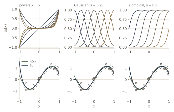
Three families of basis functions for a scalar input \(x\) come up constantly:
- Polynomials, \(\phi_j(x) = x^j\). The polynomial of module 01 is this model. Each power is nonzero almost everywhere, so every weight affects the fit over the whole input range.
- Gaussian basis functions, \(\phi_j(x) = \exp\left(-\frac{(x - \mu_j)^2}{2 s^2}\right)\): a bump at \(\mu_j\) of width \(s\). They are local, essentially zero far from their center. Nothing probabilistic is meant, and no normalizing constant is needed, because a free weight multiplies each bump anyway.
- Sigmoidal basis functions, \(\phi_j(x) = \sigma\left(\frac{x - \mu_j}{s}\right)\) with the logistic sigmoid \(\sigma(a) = 1/(1 + e^{-a})\): a smooth step located at \(\mu_j\). Since \(\tanh(a) = 2\sigma(2a) - 1\), any weighted sum of logistic steps can be rewritten as a weighted sum of tanh steps (with widths doubled and a different bias), so the two families describe the same functions.
Other choices matter in other fields. A Fourier basis of sines and cosines gives each basis function a single frequency and infinite extent, and wavelets are localized both in position and in frequency, which suits signals and images sampled on a regular grid (Bishop & Bishop §4.1.1 gives references).
Our running example has one input on \([-1, 1]\) and targets from a function we pretend not to know, \(h(x) = \sin(3x) + \tfrac12 x^2\), plus Gaussian noise of standard deviation 0.2. The design matrix \(\mathbf{\Phi}\) collects the basis functions at the training inputs: \(\Phi_{nj} = \phi_j(\mathbf{x}_n)\), so row \(n\) is \(\boldsymbol{\phi}(\mathbf{x}_n)^{\mathrm{T}}\) and \(\mathbf{\Phi}\) is \(N \times M\).
import numpy as np
from scipy.linalg import cho_factor, cho_solve, solve_triangular
from scipy.special import expit                  # logistic sigmoid 1 / (1 + exp(-a))
from scipy import integrate, optimize

np.set_printoptions(precision=4, suppress=True)
rng = np.random.default_rng(4)

SIGMA = 0.2                                      # true noise standard deviation

def h(x):
    """The true regression function E[t | x], unknown to the learner."""
    return np.sin(3 * x) + 0.5 * x**2

def make_data(N, gen, sigma=SIGMA):
    """N inputs uniform on [-1, 1] and targets h(x) + Gaussian noise."""
    x = gen.uniform(-1, 1, N)
    return x, h(x) + gen.normal(0, sigma, N)

def poly_basis(x, M):
    """Columns x, x^2, ..., x^M."""
    return x[:, None] ** np.arange(1, M + 1)

def gauss_basis(x, mu, s):
    """Columns exp(-(x - mu_j)^2 / (2 s^2)), one per center mu_j."""
    return np.exp(-(x[:, None] - mu[None, :]) ** 2 / (2 * s**2))

def sigmoid_basis(x, mu, s):
    """Columns sigma((x - mu_j) / s), one per center mu_j."""
    return expit((x[:, None] - mu[None, :]) / s)

def design_matrix(x, basis, *args):
    """N x M matrix with Phi[n, j] = phi_j(x_n); column 0 is the bias function phi_0 = 1."""
    return np.column_stack([np.ones(len(x)), basis(x, *args)])

x, t = make_data(30, rng)                        # the running data set, N = 30
MU, S = np.linspace(-1, 1, 7), 0.25              # 7 Gaussian bumps, so M = 8
Phi = design_matrix(x, gauss_basis, MU, S)
print("Phi shape:", Phi.shape)
print(f"row for x = {x[0]:.3f}:", Phi[0])
Phi shape: (30, 8)
row for x = 0.886: [1.     0.     0.     0.     0.0019 0.0868 0.6803 0.9014]
For this input near the right end of the range, only the bumps centered nearby respond; the rest of the row is close to zero. The first entry is always 1, the bias function.
Drawing the model as a network
The model \(y = \mathbf{w}^{\mathrm{T}} \boldsymbol{\phi}(\mathbf{x})\) can be drawn as a small network: one input node per basis function, one output node, and a link for each weight \(w_j\). The output node computes the weighted sum of its inputs. The first layer, which turns \(\mathbf{x}\) into \(\boldsymbol{\phi}(\mathbf{x})\), is fixed; only the one layer of links is learned. That is why Bishop & Bishop call this a single-layer network.
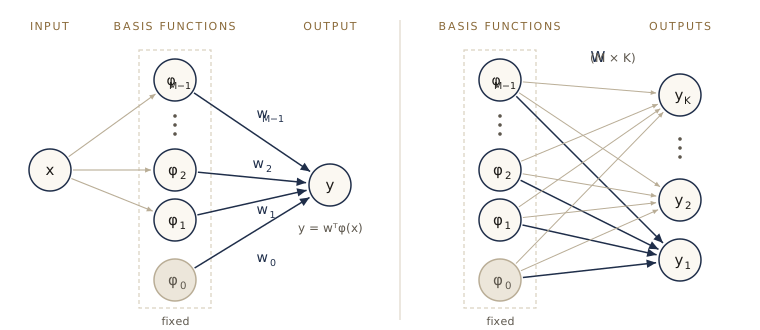
In code, the network’s forward pass is a matrix–vector product: all \(N\) outputs at once are \(\mathbf{y} = \mathbf{\Phi} \mathbf{w}\). The next cell checks this against the literal sum over links, and checks the logistic–tanh equivalence claimed above.
def forward(Phi, w):
    """Output of the single-layer network for every row of Phi: y_n = sum_j w_j phi_j(x_n)."""
    return Phi @ w

w_demo = np.linspace(-1, 1, Phi.shape[1])        # any weights will do for the check
y_links = [sum(w_demo[j] * Phi[n, j] for j in range(Phi.shape[1])) for n in range(3)]
print("forward pass:  ", forward(Phi, w_demo)[:3])
print("sum over links:", np.array(y_links))

# w_0 + sum_j w_j sigma((x - mu_j)/s)  ==  u_0 + sum_j u_j tanh((x - mu_j)/(2s))
mu, s, w = np.array([-0.5, 0.0, 0.6]), 0.1, np.array([0.3, 1.0, -2.0, 0.5])
u = np.concatenate([[w[0] + w[1:].sum() / 2], w[1:] / 2])
xs = np.linspace(-1, 1, 9)
y_sig = design_matrix(xs, sigmoid_basis, mu, s) @ w
y_tanh = np.column_stack([np.ones(9), np.tanh((xs[:, None] - mu) / (2 * s))]) @ u
print(f"logistic vs tanh network, max difference: {np.max(np.abs(y_sig - y_tanh)):.1e}")
forward pass:   [ 0.4248 -0.6949  0.3737]
sum over links: [ 0.4248 -0.6949  0.3737]
logistic vs tanh network, max difference: 2.2e-16
Fixed bases and their limits
Before deep learning, a large part of the practical work in machine learning was choosing the features \(\boldsymbol{\phi}(\mathbf{x})\) by hand, a step called feature extraction, so that a simple model on top of them would do the job. For one input variable this is easy, as the figure shows. It stops being easy quickly. Covering a \(D\)-dimensional input space with bumps the way we covered \([-1, 1]\) with seven takes \(7^D\) of them: about 2,400 for \(D = 4\), and about 282 million for \(D = 10\), while an image has thousands of input dimensions. Worse, for images, sounds, or text nobody knows how to write down features that make the task linear.
Deep learning removes this bottleneck by learning the basis functions from the data: the fixed first layer of the figure becomes one or more layers of adjustable weights. That is the subject of module 06, which also looks at the curse of dimensionality more carefully. Everything in this module still applies there to the last layer of a network, which is a linear model on learned features.
Maximum likelihood and least squares
The likelihood function
To fit the weights we need a criterion. As in module 01, assume the target is the model’s output plus Gaussian noise,
\[t = y(\mathbf{x}, \mathbf{w}) + \epsilon, \qquad \epsilon \sim \mathcal{N}(0, \sigma^2),\]so that the model defines a conditional distribution
\[p(t \mid \mathbf{x}, \mathbf{w}, \sigma^2) = \mathcal{N}\left(t \mid y(\mathbf{x}, \mathbf{w}), \sigma^2\right).\]Collect the targets in the column vector \(\mathbf{t} = (t_1, \dots, t_N)^{\mathrm{T}}\) and the inputs in \(\mathbf{X}\). If the data points are drawn independently, the likelihood is a product of Gaussians. Its logarithm, using the univariate Gaussian density, is
\[\begin{aligned} \ln p(\mathbf{t} \mid \mathbf{X}, \mathbf{w}, \sigma^2) &= \sum_{n=1}^{N} \ln \mathcal{N}\left(t_n \mid \mathbf{w}^{\mathrm{T}} \boldsymbol{\phi}(\mathbf{x}_n), \sigma^2\right) \\ &= -\frac{N}{2} \ln \sigma^2 - \frac{N}{2} \ln (2\pi) - \frac{1}{\sigma^2} E_D(\mathbf{w}), \end{aligned}\]where
\[E_D(\mathbf{w}) = \frac{1}{2} \sum_{n=1}^{N} \left\{ t_n - \mathbf{w}^{\mathrm{T}} \boldsymbol{\phi}(\mathbf{x}_n) \right\}^2 = \frac{1}{2} \lVert \mathbf{t} - \mathbf{\Phi} \mathbf{w} \rVert^2\]is the sum-of-squares error function. The first two terms do not involve \(\mathbf{w}\), so maximizing the likelihood over \(\mathbf{w}\) is the same as minimizing \(E_D\). This is the pattern for every network in the course: choose a conditional distribution for the target, and the negative log likelihood is the error function to minimize.
The normal equations
The error is a quadratic function of \(\mathbf{w}\), so we can find its minimum by setting the gradient to zero. Differentiating \(\tfrac12 \lVert \mathbf{t} - \mathbf{\Phi} \mathbf{w} \rVert^2\) gives
\[\nabla_{\mathbf{w}} E_D = -\sum_{n=1}^{N} \left\{ t_n - \mathbf{w}^{\mathrm{T}} \boldsymbol{\phi}(\mathbf{x}_n) \right\} \boldsymbol{\phi}(\mathbf{x}_n) = -\mathbf{\Phi}^{\mathrm{T}} (\mathbf{t} - \mathbf{\Phi} \mathbf{w}) .\]Setting it to zero gives the normal equations \(\mathbf{\Phi}^{\mathrm{T}} \mathbf{\Phi} \mathbf{w} = \mathbf{\Phi}^{\mathrm{T}} \mathbf{t}\). When the columns of \(\mathbf{\Phi}\) are linearly independent, \(\mathbf{\Phi}^{\mathrm{T}} \mathbf{\Phi}\) is invertible and
Result. The maximum likelihood weights of a linear model under Gaussian noise are
\[\mathbf{w}_{\mathrm{ML}} = \left(\mathbf{\Phi}^{\mathrm{T}} \mathbf{\Phi}\right)^{-1} \mathbf{\Phi}^{\mathrm{T}} \mathbf{t} = \mathbf{\Phi}^{\dagger} \mathbf{t} .\]
The \(M \times N\) matrix \(\mathbf{\Phi}^{\dagger} = (\mathbf{\Phi}^{\mathrm{T}} \mathbf{\Phi})^{-1} \mathbf{\Phi}^{\mathrm{T}}\) is the Moore–Penrose pseudo-inverse of \(\mathbf{\Phi}\). It generalizes the inverse to non-square matrices: \(\mathbf{\Phi}^{\dagger} \mathbf{\Phi} = \mathbf{I}\), and if \(\mathbf{\Phi}\) is square and invertible then \(\mathbf{\Phi}^{\dagger} = \mathbf{\Phi}^{-1}\).
Solving them in practice
Never form the inverse. There are three standard ways to compute \(\mathbf{w}_{\mathrm{ML}}\):
- Cholesky on the normal equations: factor the symmetric positive definite \(\mathbf{\Phi}^{\mathrm{T}} \mathbf{\Phi} = \mathbf{L} \mathbf{L}^{\mathrm{T}}\) and solve two triangular systems. Fast, but forming \(\mathbf{\Phi}^{\mathrm{T}} \mathbf{\Phi}\) squares the condition number.
- QR: factor \(\mathbf{\Phi} = \mathbf{Q} \mathbf{R}\) with orthonormal columns in \(\mathbf{Q}\) and upper triangular \(\mathbf{R}\). The normal equations become \(\mathbf{R} \mathbf{w} = \mathbf{Q}^{\mathrm{T}} \mathbf{t}\), one back substitution, and the condition number is that of \(\mathbf{\Phi}\) itself.
- The singular value decomposition (SVD), which is what
np.linalg.lstsquses. The most robust, and the only one of the three that handles dependent columns gracefully (below).
def fit_lstsq(Phi, t):
    """Least squares with LAPACK's SVD-based solver."""
    return np.linalg.lstsq(Phi, t, rcond=None)[0]

def fit_cholesky(Phi, t):
    """Normal equations (Phi^T Phi) w = Phi^T t, solved with a Cholesky factorization."""
    return cho_solve(cho_factor(Phi.T @ Phi), Phi.T @ t)

def fit_qr(Phi, t):
    """Phi = QR, then R w = Q^T t by back substitution."""
    Q, R = np.linalg.qr(Phi)
    return solve_triangular(R, Q.T @ t)

w_ml = fit_qr(Phi, t)
print("w_ML:", w_ml)
for name, fit in [("lstsq", fit_lstsq), ("Cholesky", fit_cholesky)]:
    print(f"max |w_{name} - w_QR| = {np.max(np.abs(fit(Phi, t) - w_ml)):.1e}")
grad = -Phi.T @ (t - forward(Phi, w_ml))
print(f"largest gradient component at w_ML: {np.max(np.abs(grad)):.1e}")
print(f"cond(Phi) = {np.linalg.cond(Phi):.0f},"
      f"  cond(Phi^T Phi) = {np.linalg.cond(Phi.T @ Phi):.1e}")
w_ML: [-2.4485  2.1452  0.6118  0.7357  1.3243  1.8126  1.9978  1.9962]
max |w_lstsq - w_QR| = 3.1e-15
max |w_Cholesky - w_QR| = 7.6e-13
largest gradient component at w_ML: 1.1e-14
cond(Phi) = 205,  cond(Phi^T Phi) = 4.2e+04
The three solvers agree, and the gradient vanishes at the solution to rounding error. Look at the weights, though: the bias is large and negative while the bump weights are all positive. Seven overlapping bumps add up to something close to a constant on \([-1, 1]\), so the bias column and the sum of the bump columns are nearly interchangeable, and the fit trades one against the other. The condition number of \(\mathbf{\Phi}^{\mathrm{T}} \mathbf{\Phi}\) measures this near-degeneracy; it will come back when we train by gradient descent.
In the extreme, two basis functions coincide. Let us add a copy of column 3 (the third bump) and see what the solvers do.
Phi_twin = np.column_stack([Phi, Phi[:, 3]])             # an exact copy of column 3
print(f"rank {np.linalg.matrix_rank(Phi_twin)} with {Phi_twin.shape[1]} columns;"
      f" smallest singular values {np.linalg.svd(Phi_twin, compute_uv=False)[-2:]}")
try:
    fit_cholesky(Phi_twin, t)
except np.linalg.LinAlgError as err:
    print("normal equations with Cholesky:", err)
w_svd = fit_lstsq(Phi_twin, t)                           # SVD: minimum-norm solution
A_tiny = Phi_twin.T @ Phi_twin + 1e-6 * np.eye(Phi_twin.shape[1])   # add a tiny multiple of I
w_tiny = cho_solve(cho_factor(A_tiny), Phi_twin.T @ t)
for name, w in [("SVD (lstsq)", w_svd), ("Cholesky + 1e-6 I", w_tiny)]:
    change = np.max(np.abs(forward(Phi_twin, w) - forward(Phi, w_ml)))
    print(f"{name:18s} twin weights {w[3]:.4f} {w[-1]:.4f}  (w_ML: {w_ml[3]:.4f})"
          f"   max change in fit {change:.1e}")
rank 8 with 9 columns; smallest singular values [0.0339 0.    ]
normal equations with Cholesky: 9-th leading minor of the array is not positive definite
SVD (lstsq)        twin weights 0.3678 0.3678  (w_ML: 0.7357)   max change in fit 2.7e-15
Cholesky + 1e-6 I  twin weights 0.3672 0.3672  (w_ML: 0.7357)   max change in fit 7.0e-05
With a repeated column, \(\mathbf{\Phi}^{\mathrm{T}} \mathbf{\Phi}\) is singular and the Cholesky factorization stops. The fitted values are still perfectly well defined, since the column space has not changed; only the split of the weight between the twins is not. The SVD-based solver returns the minimum-norm solution, which splits the old weight evenly between the twins and leaves the fit unchanged. Adding a tiny multiple of the identity to \(\mathbf{\Phi}^{\mathrm{T}} \mathbf{\Phi}\) does almost the same thing, and is a preview of the regularizer below. With two nearly identical columns, the normal equations would not fail outright; instead they would return huge weights of opposite sign whose difference exploits the tiny direction separating the twins, and with a squared condition number they would lose most of their accuracy doing it.
The bias and the noise variance
The bias weight has a direct interpretation. Write \(w_0\) out of the sum in \(E_D\) and set the derivative with respect to \(w_0\) to zero:
\[w_0 = \bar{t} - \sum_{j=1}^{M-1} w_j \bar{\phi}_j, \qquad \bar{t} = \frac{1}{N} \sum_{n=1}^{N} t_n, \quad \bar{\phi}_j = \frac{1}{N} \sum_{n=1}^{N} \phi_j(\mathbf{x}_n).\]The bias makes up the difference between the average target and the weighted average of the other basis functions. So the residuals of a least-squares fit with a bias always average to zero.
Maximizing the log likelihood over \(\sigma^2\) as well: its derivative with respect to \(\sigma^2\) is \(-\frac{N}{2\sigma^2} + \frac{E_D}{\sigma^4}\), which vanishes at
\[\sigma^2_{\mathrm{ML}} = \frac{1}{N} \sum_{n=1}^{N} \left\{ t_n - \mathbf{w}_{\mathrm{ML}}^{\mathrm{T}} \boldsymbol{\phi}(\mathbf{x}_n) \right\}^2 ,\]the mean squared residual around the fitted function.
N, M = Phi.shape
resid = t - forward(Phi, w_ml)
w0_formula = t.mean() - w_ml[1:] @ Phi[:, 1:].mean(axis=0)
sigma2_ml = np.mean(resid**2)
loglik = -N / 2 * np.log(sigma2_ml) - N / 2 * np.log(2 * np.pi) - 0.5 * resid @ resid / sigma2_ml
loglik_terms = np.sum(-0.5 * np.log(2 * np.pi * sigma2_ml) - resid**2 / (2 * sigma2_ml))
print(f"w0 from the solver {w_ml[0]:.4f},  from the averages {w0_formula:.4f}")
print(f"mean residual {resid.mean():.1e}")
print(f"sigma^2_ML = {sigma2_ml:.4f}   true sigma^2 = {SIGMA**2:.4f}")
print(f"log likelihood at the optimum: {loglik:.4f} (formula), {loglik_terms:.4f} (sum of terms)")
w0 from the solver -2.4485,  from the averages -2.4485
mean residual -3.6e-16
sigma^2_ML = 0.0240   true sigma^2 = 0.0400
log likelihood at the optimum: 13.3823 (formula), 13.3823 (sum of terms)
The noise estimate comes out below the true variance. That is typical: the fit has used its \(M = 8\) parameters to follow some of the noise, so the residuals are smaller than the real noise. (For a model that contains the true function, the expected value of \(\sigma^2_{\mathrm{ML}}\) is \(\frac{N - M}{N} \sigma^2\), the same bias as dividing by \(N\) instead of \(N - 1\) for a sample variance.)
The geometry of least squares
Least squares has a picture that is worth having in mind. Think of the target vector \(\mathbf{t}\) as a point in \(N\)-dimensional space, one axis per data point. Each basis function evaluated at the \(N\) inputs is also a vector in that space: the \(j\)th column of \(\mathbf{\Phi}\), which we write \(\boldsymbol{\varphi}_j\) (not to be confused with \(\boldsymbol{\phi}(\mathbf{x}_n)\), which is a row). The network’s outputs on the training set,
\[\mathbf{y} = \mathbf{\Phi} \mathbf{w} = \sum_{j=0}^{M-1} w_j \boldsymbol{\varphi}_j ,\]can be any point of the subspace \(\mathcal{S}\) spanned by the columns, which has dimension \(M\) when the columns are independent and \(M < N\). Since \(E_D = \tfrac12 \lVert \mathbf{t} - \mathbf{y} \rVert^2\), least squares picks the point of \(\mathcal{S}\) closest to \(\mathbf{t}\), and the closest point of a subspace is the orthogonal projection.
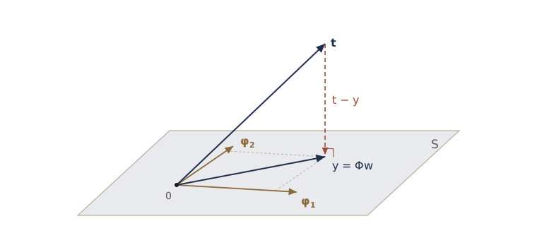
The normal equations say exactly this. \(\mathbf{\Phi}^{\mathrm{T}} (\mathbf{t} - \mathbf{\Phi} \mathbf{w}_{\mathrm{ML}}) = \mathbf{0}\) states that the residual has zero dot product with every column \(\boldsymbol{\varphi}_j\), so it is orthogonal to \(\mathcal{S}\). And the fitted outputs are
\[\mathbf{y} = \mathbf{\Phi} \mathbf{w}_{\mathrm{ML}} = \mathbf{\Phi} \left(\mathbf{\Phi}^{\mathrm{T}} \mathbf{\Phi}\right)^{-1} \mathbf{\Phi}^{\mathrm{T}} \mathbf{t} = \mathbf{P} \mathbf{t}, \qquad \mathbf{P} = \mathbf{\Phi} \mathbf{\Phi}^{\dagger},\]where the \(N \times N\) matrix \(\mathbf{P}\) is the projection onto \(\mathcal{S}\). A projection matrix is symmetric, satisfies \(\mathbf{P}^2 = \mathbf{P}\) (projecting twice changes nothing), and has trace equal to the dimension of the subspace. With the QR factorization, \(\mathbf{P} = \mathbf{Q} \mathbf{Q}^{\mathrm{T}}\), which is how we compute it.
The smallest case we can picture has \(N = 3\) data points and \(M = 2\) basis functions (a bias and \(x\)), so \(\mathbf{t}\) lives in three dimensions and \(\mathcal{S}\) is a plane, exactly as in the figure. We check the picture there, and then on the running data.
x3 = np.array([-0.6, 0.1, 0.8])
t3 = np.array([-0.5, 0.6, 0.4])
Phi3 = design_matrix(x3, poly_basis, 1)          # columns: phi_0 = 1 and phi_1 = x
y3 = forward(Phi3, fit_qr(Phi3, t3))
r3 = t3 - y3
print("t =", t3, "  y =", y3, "  t - y =", r3)
print("dot products of t - y with the two columns:", Phi3.T @ r3)

y = forward(Phi, w_ml)
r = t - y
Q, _ = np.linalg.qr(Phi)
P = Q @ Q.T                                      # projection onto the column space S
print(f"running data: largest |phi_j . (t - y)| = {np.max(np.abs(Phi.T @ r)):.1e}")
print(f"P symmetric: {np.allclose(P, P.T)},  P @ P == P: {np.allclose(P @ P, P)},  "
      f"trace(P) = {np.trace(P):.4f},  P t == y: {np.allclose(P @ t, y)}")
print(f"||t||^2 = {t @ t:.4f}   ||y||^2 + ||t - y||^2 = {y @ y + r @ r:.4f}")
t = [-0.5  0.6  0.4]   y = [-0.2833  0.1667  0.6167]   t - y = [-0.2167  0.4333 -0.2167]
dot products of t - y with the two columns: [ 0. -0.]
running data: largest |phi_j . (t - y)| = 1.1e-14
P symmetric: True,  P @ P == P: True,  trace(P) = 8.0000,  P t == y: True
||t||^2 = 15.4626   ||y||^2 + ||t - y||^2 = 15.4626
In three dimensions the residual is visibly perpendicular to both columns. On the running data the projection matrix is symmetric and idempotent with trace \(M = 8\), and Pythagoras holds for \(\mathbf{t}\), \(\mathbf{y}\), and the residual.
The picture also explains the twin-column experiment. When two columns point in almost the same direction, the plane they span is still well defined, and so is the projection \(\mathbf{y}\). What is not well defined is how to write \(\mathbf{y}\) as a combination of two nearly parallel vectors: many pairs of coefficients, some of them huge, give almost the same point. The fit is stable; the weights are not.
Sequential learning
Stochastic gradient descent and the LMS rule
The closed-form solution processes the whole training set at once; it is a batch method. For a network with millions of data points, or data that arrive in a stream, we want to update the weights a little after each data point, or each small group of points. This is sequential (or online) learning.
Any error that is a sum over data points, \(E(\mathbf{w}) = \sum_n E_n(\mathbf{w})\), can be minimized this way. Stochastic gradient descent (SGD) picks a data point \(n\) and takes a small step against the gradient of its term alone,
\[\mathbf{w}^{(\tau+1)} = \mathbf{w}^{(\tau)} - \eta \nabla E_n\left(\mathbf{w}^{(\tau)}\right),\]where \(\tau\) counts the updates and \(\eta > 0\) is the learning rate. For the sum-of-squares error, \(E_n = \tfrac12 (t_n - \mathbf{w}^{\mathrm{T}} \boldsymbol{\phi}_n)^2\) with \(\boldsymbol{\phi}_n = \boldsymbol{\phi}(\mathbf{x}_n)\), and \(\nabla E_n = -(t_n - \mathbf{w}^{\mathrm{T}} \boldsymbol{\phi}_n) \boldsymbol{\phi}_n\), so
\[\mathbf{w}^{(\tau+1)} = \mathbf{w}^{(\tau)} + \eta \left(t_n - \mathbf{w}^{(\tau)\mathrm{T}} \boldsymbol{\phi}_n\right) \boldsymbol{\phi}_n .\]This is the least-mean-squares (LMS) algorithm. In network terms: run the input forward, compare the output with the target, and move each weight \(w_j\) in proportion to the error times the activity \(\phi_j(\mathbf{x}_n)\) at the input end of its link. Using a small group of points, a mini-batch, instead of one point averages out some of the randomness in each step; using all \(N\) points gives batch gradient descent.
A training loop
Here is that procedure written as the training loop we will use, with small changes, for every network in the course. One epoch is one pass through the training set in a fresh random order. The lam argument adds a penalty \(\tfrac{\lambda}{2} \mathbf{w}^{\mathrm{T}} \mathbf{w}\) that we need in the section on regularization; it is shared evenly among the \(N\) data points, \(E_n = \tfrac12 (t_n - \mathbf{w}^{\mathrm{T}} \boldsymbol{\phi}_n)^2 + \tfrac{\lambda}{2N} \mathbf{w}^{\mathrm{T}} \mathbf{w}\), so that the terms still add up to the whole error.
def train(Phi, t, eta, epochs, gen, batch_size=1, lam=0.0, tau0=None, w_ref=None):
    """Mini-batch stochastic gradient descent on E(w) = E_D(w) + (lam/2) w^T w.

    The step size is eta, or eta / (1 + tau / tau0) when tau0 is given (a decaying schedule).
    Returns the final weights and, if w_ref is given, ||w - w_ref|| after every epoch.
    """
    N, M = Phi.shape
    w = np.zeros(M)                                        # w^(0) = 0
    tau, dist = 0, []
    for epoch in range(epochs):
        order = gen.permutation(N)                         # a fresh pass through the data
        for start in range(0, N, batch_size):
            b = order[start:start + batch_size]
            err = t[b] - forward(Phi[b], w)                # forward pass and errors t_n - y_n
            grad = -Phi[b].T @ err + lam * len(b) / N * w  # gradient of the batch's share of E
            step = eta if tau0 is None else eta / (1 + tau / tau0)
            w = w - step * grad                            # w^(tau+1) = w^(tau) - eta grad
            tau += 1
        if w_ref is not None:
            dist.append(np.linalg.norm(w - w_ref))
    return w, np.array(dist)
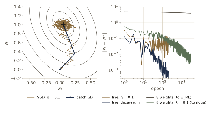
To see the loop at work, start with the smallest network there is: a bias and one input, \(y = w_0 + w_1 x\), a straight line fitted to the running data. With only two weights we can draw the error surface and the paths the optimizers take.
Phi_line = design_matrix(x, poly_basis, 1)                 # phi_0 = 1, phi_1 = x
w_line = fit_qr(Phi_line, t)
lam_max = np.linalg.eigvalsh(Phi_line.T @ Phi_line)[-1]
print("closed form w =", w_line, f"  largest eigenvalue of Phi^T Phi: {lam_max:.2f}",
      f"  max ||phi_n||^2: {np.max(np.sum(Phi_line**2, axis=1)):.2f}")
runs = [("batch GD, eta = 1 / lam_max", dict(eta=1 / lam_max, batch_size=30)),
        ("SGD, eta = 0.1", dict(eta=0.1)),
        ("SGD, eta = 0.3 / (1 + tau/100)", dict(eta=0.3, tau0=100)),
        ("SGD, eta = 1.2", dict(eta=1.2))]
print("distance ||w - w_closed|| after epoch")
print(f"{'':32s}" + "".join(f"{e:>10d}" for e in (1, 10, 50, 200)))
for name, kw in runs:
    _, d = train(Phi_line, t, epochs=200, gen=np.random.default_rng(0), w_ref=w_line, **kw)
    print(f"{name:32s}" + "".join(f"{d[e - 1]:10.1e}" for e in (1, 10, 50, 200)))
closed form w = [0.0531 1.0059]   largest eigenvalue of Phi^T Phi: 31.71   max ||phi_n||^2: 1.94
distance ||w - w_closed|| after epoch
                                         1        10        50       200
batch GD, eta = 1 / lam_max        6.8e-01   3.3e-02   4.7e-08   4.4e-16
SGD, eta = 0.1                     3.3e-01   1.2e-01   1.9e-02   7.6e-02
SGD, eta = 0.3 / (1 + tau/100)     1.3e-01   8.3e-02   3.2e-03   8.9e-04
SGD, eta = 1.2                     7.4e-01   3.8e-01   5.4e-01   1.3e-01
Batch gradient descent with a safe step converges to the closed-form solution geometrically, down to rounding error. SGD with a fixed learning rate gets close quickly and then stops improving: every step chases a single data point, so the weights keep jittering in a neighborhood of \(\mathbf{w}_{\mathrm{ML}}\) whose size is set by \(\eta\). With a learning rate that decays over time, the jitter dies down and SGD converges too. A decaying schedule converges when the steps shrink, but slowly enough that their sum is still infinite: \(\sum_\tau \eta_\tau = \infty\) and \(\sum_\tau \eta_\tau^2 < \infty\) (the Robbins–Monro conditions). The schedule \(\eta_0 / (1 + \tau/\tau_0)\) satisfies both.
Learning rates
The learning rate is the one number that most decides whether gradient training works. For batch gradient descent on a quadratic error we can see exactly why. Near the minimum, \(E_D(\mathbf{w}) = E_D(\mathbf{w}_{\mathrm{ML}}) + \tfrac12 (\mathbf{w} - \mathbf{w}_{\mathrm{ML}})^{\mathrm{T}} \mathbf{H} (\mathbf{w} - \mathbf{w}_{\mathrm{ML}})\) with the Hessian \(\mathbf{H} = \mathbf{\Phi}^{\mathrm{T}} \mathbf{\Phi}\) (here the expansion is exact). One gradient step maps the error vector \(\mathbf{w} - \mathbf{w}_{\mathrm{ML}}\) to \((\mathbf{I} - \eta \mathbf{H})(\mathbf{w} - \mathbf{w}_{\mathrm{ML}})\). Along an eigenvector \(\mathbf{u}_i\) of \(\mathbf{H}\) with eigenvalue \(\lambda_i\) the component is multiplied by \(1 - \eta \lambda_i\) at every step. Two consequences follow.
- Stability. Every factor must have magnitude below 1, which requires \(\eta < 2 / \lambda_{\max}\). Above that, the steepest direction overshoots further each step and the weights blow up.
- Speed. The slowest direction shrinks by \(1 - \eta \lambda_{\min}\) per step. With the largest safe \(\eta\) that is roughly \(1 - 2/\kappa\), where \(\kappa = \lambda_{\max} / \lambda_{\min}\) is the condition number of \(\mathbf{H}\), so reducing the error by a fixed factor takes a number of steps proportional to \(\kappa\).
For SGD with single points the analogous stability condition involves one data point: an update changes that point’s own prediction error by the factor \(1 - \eta \lVert \boldsymbol{\phi}_n \rVert^2\), so \(\eta \lVert \boldsymbol{\phi}_n \rVert^2 > 2\) makes the step overshoot. In the run above, \(\eta = 1.2\) pushes \(\eta \lVert \boldsymbol{\phi}_n \rVert^2\) above 2 for the points with \(\lvert x_n \rvert\) above about 0.8, and the distance to the closed form jumps around at the level of tenths instead of shrinking. The next cell sweeps the batch learning rate across the stability limit.
evals_line = np.linalg.eigvalsh(Phi_line.T @ Phi_line)
print(f"eigenvalues of H: {evals_line},  2 / lam_max = {2 / lam_max:.4f}")
print("eta * lam_max   ||w - w_closed|| after 5, 20, 100 steps")
for c in [0.05, 0.5, 1.0, 1.9, 2.05]:
    _, d = train(Phi_line, t, eta=c / lam_max, epochs=100, batch_size=30,
                 gen=np.random.default_rng(0), w_ref=w_line)
    print(f"{c:10.2f}       " + "   ".join(f"{d[k - 1]:9.2e}" for k in (5, 20, 100)))
eigenvalues of H: [ 9.0605 31.7138],  2 / lam_max = 0.0631
eta * lam_max   ||w - w_closed|| after 5, 20, 100 steps
      0.05        9.22e-01    7.24e-01    2.26e-01
      0.50        4.41e-01    4.37e-02    1.93e-07
      1.00        1.77e-01    1.14e-03    2.29e-15
      1.90        1.94e-01    3.98e-02    8.71e-06
      2.05        4.18e-01    8.70e-01    4.31e+01
A tiny step converges but slowly, a step near \(1/\lambda_{\max}\) converges fastest here, a step just under the limit oscillates while converging, and a step just over it diverges. Nothing about the data changed; only \(\eta\) did.
What gradient descent struggles with
The straight line is an easy case: its Hessian has a condition number of about 3.5. Now train the eight-parameter Gaussian model on the same data by SGD, with a decaying learning rate, for 3000 epochs.
w_sgd, d_sgd = train(Phi, t, eta=0.5, epochs=3000, gen=np.random.default_rng(1),
                     tau0=3000, w_ref=w_ml)

def E_D(Phi, t, w):
    """Sum-of-squares error 1/2 ||t - Phi w||^2."""
    return 0.5 * np.sum((t - forward(Phi, w)) ** 2)

evals, U = np.linalg.eigh(Phi.T @ Phi)                     # eigenvalues in increasing order
print("||w - w_ML|| after epochs 1, 10, 100, 1000, 3000:", d_sgd[[0, 9, 99, 999, 2999]])
print(f"E_D(w_SGD) - E_D(w_ML) = {E_D(Phi, t, w_sgd) - E_D(Phi, t, w_ml):.4f}"
      f"   (E_D(w_ML) = {E_D(Phi, t, w_ml):.4f})")
print("eigenvalues of H:            ", evals)
print("components of w_SGD - w_ML:  ", U.T @ (w_sgd - w_ml))
print("flattest direction u_1:      ", U[:, 0])
||w - w_ML|| after epochs 1, 10, 100, 1000, 3000: [4.7952 4.7229 4.5823 4.1545 3.9199]
E_D(w_SGD) - E_D(w_ML) = 0.0105   (E_D(w_ML) = 0.3599)
eigenvalues of H:             [ 0.0011  0.1146  0.2892  0.9696  2.9282  7.1104 12.2692 45.7342]
components of w_SGD - w_ML:   [ 3.9199 -0.0008 -0.0001  0.0002 -0.0015 -0.0002 -0.0007 -0.0095]
flattest direction u_1:       [ 0.5473 -0.3705 -0.2591 -0.3122 -0.2697 -0.3234 -0.2332 -0.4085]
After 3000 epochs (90,000 updates) the weights are still almost 4 away from \(\mathbf{w}_{\mathrm{ML}}\), having closed only about a fifth of the initial gap of 4.95, yet the error exceeds its minimum by only about 0.01, some 3% of \(E_D(\mathbf{w}_{\mathrm{ML}})\). The eigen-decomposition says why. The Hessian’s eigenvalues span more than four orders of magnitude, and almost all of the remaining difference lies along the eigenvector \(\mathbf{u}_1\) with the smallest eigenvalue. That vector raises the bias while lowering every bump weight: it is the near-degenerate direction where the bias and the sum of the bumps trade off. Along it the error surface is so flat that the gradient hardly pulls, and moving along it hardly changes the predictions. Every other component has converged.
Note. This is the central difficulty of training networks by gradient descent, seen here in its simplest form: the error surface is steep in some directions and nearly flat in others, and a single learning rate cannot suit both. Module 07 takes it up with momentum, adaptive learning rates (RMSProp, Adam), and normalization of the inputs to each layer, all of which improve the conditioning that the optimizer sees.
Regularized least squares
Quadratic regularization and weight decay
Module 01 controlled overfitting by adding a penalty on the weights to the error. In general we minimize
\[E(\mathbf{w}) = E_D(\mathbf{w}) + \lambda E_W(\mathbf{w}),\]where \(E_W\) is a regularizer and the regularization coefficient \(\lambda \ge 0\) sets its importance relative to the data. The simplest regularizer is half the sum of the squared weights, \(E_W(\mathbf{w}) = \tfrac12 \mathbf{w}^{\mathrm{T}} \mathbf{w}\). Statisticians call it ridge regression, a parameter shrinkage method because it pulls the weights toward zero. In neural networks it is called weight decay, because its gradient \(\lambda \mathbf{w}\) adds a step \(-\eta \lambda \mathbf{w}\) to every update, shrinking each weight by a constant fraction unless the data push back.
The total error is still quadratic, with gradient \(-\mathbf{\Phi}^{\mathrm{T}}(\mathbf{t} - \mathbf{\Phi} \mathbf{w}) + \lambda \mathbf{w}\). Setting it to zero gives
\[\mathbf{w} = \left(\lambda \mathbf{I} + \mathbf{\Phi}^{\mathrm{T}} \mathbf{\Phi}\right)^{-1} \mathbf{\Phi}^{\mathrm{T}} \mathbf{t} .\]Every eigenvalue of \(\lambda \mathbf{I} + \mathbf{\Phi}^{\mathrm{T}} \mathbf{\Phi}\) is its counterpart in \(\mathbf{\Phi}^{\mathrm{T}} \mathbf{\Phi}\) plus \(\lambda\). So for any \(\lambda > 0\) the matrix is positive definite, even with dependent columns or \(M > N\), and its condition number is at most \((\lambda_{\max} + \lambda)/\lambda\). That is good news for both kinds of solver: Cholesky becomes safe, and gradient descent no longer has a nearly flat direction to crawl along.
Two numerical checks: the closed form agrees with ordinary least squares on augmented data (append \(\sqrt{\lambda}\, \mathbf{I}\) as \(M\) extra rows of \(\mathbf{\Phi}\) and \(M\) zeros to \(\mathbf{t}\), and \(\lVert \tilde{\mathbf{t}} - \tilde{\mathbf{\Phi}} \mathbf{w} \rVert^2\) becomes the ridge error), and our training loop with lam set converges to it.
def fit_ridge(Phi, t, lam):
    """(lam I + Phi^T Phi)^{-1} Phi^T t with a Cholesky factorization (lam > 0)."""
    A = lam * np.eye(Phi.shape[1]) + Phi.T @ Phi
    return cho_solve(cho_factor(A), Phi.T @ t)

lam = 0.1
w_ridge = fit_ridge(Phi, t, lam)
w_aug = fit_qr(np.vstack([Phi, np.sqrt(lam) * np.eye(M)]), np.concatenate([t, np.zeros(M)]))
print(f"ridge closed form vs augmented least squares: {np.max(np.abs(w_ridge - w_aug)):.1e}")
w_wd, d_wd = train(Phi, t, eta=0.5, epochs=3000, gen=np.random.default_rng(1),
                   lam=lam, tau0=3000, w_ref=w_ridge)
print("SGD with weight decay, ||w - w_ridge|| after epochs 1, 10, 100, 1000, 3000:",
      d_wd[[0, 9, 99, 999, 2999]])

x_grid = np.linspace(-1, 1, 401)
Phi_grid = design_matrix(x_grid, gauss_basis, MU, S)
print(" ln lambda   ||w||   train RMS   RMS vs h(x)   cond(lam I + H)")
for ln_lam in [-np.inf, -6, -3, -1, 1, 3]:
    lam_k = np.exp(ln_lam)
    w_k = w_ml if lam_k == 0 else fit_ridge(Phi, t, lam_k)
    rms_train = np.sqrt(np.mean((t - forward(Phi, w_k)) ** 2))
    rms_true = np.sqrt(np.mean((h(x_grid) - forward(Phi_grid, w_k)) ** 2))
    cond = np.linalg.cond(lam_k * np.eye(M) + Phi.T @ Phi)
    print(f"{ln_lam:9.0f}   {np.linalg.norm(w_k):6.3f}    {rms_train:.4f}      {rms_true:.4f}"
          f"        {cond:.1e}")
ridge closed form vs augmented least squares: 7.0e-15
SGD with weight decay, ||w - w_ridge|| after epochs 1, 10, 100, 1000, 3000: [0.5598 0.2718 0.1538 0.0126 0.0106]
 ln lambda   ||w||   train RMS   RMS vs h(x)   cond(lam I + H)
     -inf    4.953    0.1549      0.0772        4.2e+04
       -6    2.021    0.1562      0.0599        1.3e+04
       -3    1.346    0.1579      0.0550        9.0e+02
       -1    1.179    0.1652      0.0869        1.2e+02
        1    0.898    0.2280      0.2250        1.8e+01
        3    0.397    0.4697      0.5187        3.3e+00
With \(\lambda = 0.1\), the same SGD run that crawled toward \(\mathbf{w}_{\mathrm{ML}}\) gets within about 0.01 of the ridge weights in 1000 epochs, because the flat direction has been lifted; what remains is SGD’s own jitter. The table shows what \(\lambda\) does to the fit. As it grows, the weights shrink, the training error rises, and the condition number falls. The error against the true function \(h\), which we can compute only because we made up the data, is smallest at a moderate \(\lambda\): too little regularization lets the fit follow noise, too much flattens it. Choosing \(\lambda\) is therefore the question of model complexity in a new form. Note that minimizing \(E(\mathbf{w})\) over \(\lambda\) as well as \(\mathbf{w}\) would always pick \(\lambda = 0\), since the penalty only adds to the error. The bias–variance section below looks at the trade-off, and module 09 treats weight decay and its alternatives for deep networks.
Other penalties and sparsity
The quadratic penalty is one member of a family, \(E_W(\mathbf{w}) = \tfrac12 \sum_j \lvert w_j \rvert^q\). The case \(q = 1\) is the lasso. Its notable property is sparsity: for a large enough \(\lambda\), some weights are driven to exactly zero, and their basis functions drop out of the model.
The simplest way to see why is a design matrix with orthonormal columns, \(\mathbf{\Phi}^{\mathrm{T}} \mathbf{\Phi} = \mathbf{I}\). Then the error separates into one term per weight, \(\tfrac12 (w_j - a_j)^2 + \tfrac{\lambda}{2} \lvert w_j \rvert^q\) plus a constant, where \(a_j = \boldsymbol{\varphi}_j^{\mathrm{T}} \mathbf{t}\) is the unregularized solution. For \(q = 2\) the minimizer is \(w_j = a_j / (1 + \lambda)\): every weight is scaled down, none reaches zero. For \(q = 1\), on each side of zero the derivative is \(w_j - a_j \pm \lambda/2\), and the minimizer is the soft-thresholding of \(a_j\),
\[w_j = \operatorname{sign}(a_j) \max\left(\lvert a_j \rvert - \tfrac{\lambda}{2},\, 0\right):\]every weight is moved toward zero by the same amount, and those within \(\lambda/2\) of zero land exactly on it. The kink of \(\lvert w \rvert\) at zero is what makes zero a stable answer. For \(q < 1\) the effect is stronger still, but the penalty is no longer convex.
For a general design matrix there is no closed form, but gradient descent extends naturally. Proximal gradient descent (also known as ISTA) alternates a gradient step on the smooth part \(E_D\) with the soft-thresholding that solves the penalty part exactly:
\[\mathbf{w} \leftarrow \operatorname{soft}\left(\mathbf{w} - \eta \nabla E_D(\mathbf{w}),\; \eta \lambda / 2\right), \qquad \eta = 1 / \lambda_{\max}(\mathbf{H}).\]We try it on a richer set of features, 21 narrow bumps, and check the answer with the optimality conditions of the lasso: with \(\mathbf{g} = \mathbf{\Phi}^{\mathrm{T}} (\mathbf{t} - \mathbf{\Phi} \mathbf{w})\), each nonzero weight needs \(g_j = \tfrac{\lambda}{2} \operatorname{sign}(w_j)\) and each zero weight needs \(\lvert g_j \rvert \le \tfrac{\lambda}{2}\).
def soft(a, c):
    """Soft thresholding: move a toward zero by c and clip at zero."""
    return np.sign(a) * np.maximum(np.abs(a) - c, 0.0)

def fit_l1(Phi, t, lam, max_iters=50000, tol=1e-10):
    """Minimize E_D(w) + (lam/2) sum_j |w_j| by proximal gradient descent (ISTA).
    Stops when no weight changes by more than tol; returns w and the number of iterations."""
    eta = 1 / np.linalg.eigvalsh(Phi.T @ Phi)[-1]
    w = np.zeros(Phi.shape[1])
    for it in range(1, max_iters + 1):
        w_new = soft(w + eta * Phi.T @ (t - forward(Phi, w)), eta * lam / 2)
        if np.max(np.abs(w_new - w)) < tol:
            return w_new, it
        w = w_new
    return w, max_iters

def l1_violation(Phi, t, w, lam):
    """Largest violation of the lasso optimality conditions (zero at the exact minimum)."""
    g = Phi.T @ (t - forward(Phi, w))
    nz = w != 0
    return max(np.max(np.abs(g[nz] - lam / 2 * np.sign(w[nz])), initial=0.0),
               np.max(np.abs(g[~nz]) - lam / 2, initial=0.0))

Phi21 = design_matrix(x, gauss_basis, np.linspace(-1, 1, 21), 0.15)
print("   lambda   nonzero of 22   iterations   violation   train RMS   ridge nonzero")
for lam_k in [0.01, 0.1, 0.5, 2.0, 5.0]:
    w_k, its = fit_l1(Phi21, t, lam_k)
    rms = np.sqrt(np.mean((t - forward(Phi21, w_k)) ** 2))
    n_ridge = np.sum(fit_ridge(Phi21, t, lam_k) != 0)
    viol = l1_violation(Phi21, t, w_k, lam_k)
    print(f"{lam_k:9.2f}   {np.sum(w_k != 0):8d}      {its:9d}    {viol:8.1e}"
          f"     {rms:.4f}        {n_ridge}")
   lambda   nonzero of 22   iterations   violation   train RMS   ridge nonzero
     0.01         12          50000     1.5e-06     0.1463        22
     0.10         10          50000     3.8e-08     0.1555        22
     0.50          8          36944     5.1e-09     0.1634        22
     2.00          5           6363     5.0e-09     0.2464        22
     5.00          5           3149     5.1e-09     0.4886        22
As \(\lambda\) grows, the L1 penalty switches off more and more bumps, from 12 of 22 left at \(\lambda = 0.01\) to 5 at \(\lambda = 2\) and beyond, while the fit to the training data degrades gracefully. The optimality conditions hold to about \(10^{-6}\) or better, so ISTA has found the minimum. Notice the iteration counts: at small \(\lambda\), where many overlapping bumps stay active, ISTA uses its whole budget of 50,000 steps, for the same conditioning reason that slowed SGD; with few active bumps it finishes in a few thousand. Ridge with the same \(\lambda\) keeps every weight nonzero. Sparse penalties and the geometry behind them are discussed further in Bishop & Bishop §9.2.2 and in Intro to ML, module 03, which solves the lasso by coordinate descent.
In practice. Deep networks mostly use the quadratic penalty, usually in the form of weight decay inside the optimizer. L1 penalties appear when sparsity itself is the goal, for example to select a few inputs or to prune connections, and a proximal step like the one above is a standard way to handle their kink inside a gradient method.
Multiple outputs
Sometimes we want to predict \(K > 1\) targets at once, collected in a vector \(\mathbf{t}\). We could fit a separate model, with its own basis functions, for each. The usual choice, and the one that matches the network picture, is to share the basis functions and give each output its own weights:
\[\mathbf{y}(\mathbf{x}, \mathbf{W}) = \mathbf{W}^{\mathrm{T}} \boldsymbol{\phi}(\mathbf{x}),\]where \(\mathbf{W}\) is an \(M \times K\) matrix whose column \(k\) holds the weights into output \(k\) (the right half of the network figure). Take isotropic Gaussian noise, \(p(\mathbf{t} \mid \mathbf{x}, \mathbf{W}, \sigma^2) = \mathcal{N}(\mathbf{t} \mid \mathbf{W}^{\mathrm{T}} \boldsymbol{\phi}(\mathbf{x}), \sigma^2 \mathbf{I})\), and stack the target vectors as the rows of an \(N \times K\) matrix \(\mathbf{T}\). The log likelihood is
\[\ln p(\mathbf{T} \mid \mathbf{X}, \mathbf{W}, \sigma^2) = -\frac{NK}{2} \ln (2\pi\sigma^2) - \frac{1}{2\sigma^2} \sum_{n=1}^{N} \left\lVert \mathbf{t}_n - \mathbf{W}^{\mathrm{T}} \boldsymbol{\phi}(\mathbf{x}_n) \right\rVert^2 .\]The squared norm is a sum over the \(K\) components, and component \(k\) involves only column \(k\) of \(\mathbf{W}\). So the problem splits into \(K\) independent least-squares problems with the same design matrix,
\[\mathbf{W}_{\mathrm{ML}} = \left(\mathbf{\Phi}^{\mathrm{T}} \mathbf{\Phi}\right)^{-1} \mathbf{\Phi}^{\mathrm{T}} \mathbf{T} = \mathbf{\Phi}^{\dagger} \mathbf{T},\]and one factorization of \(\mathbf{\Phi}\) serves all of them.
What if the noise on the outputs is correlated, with a full covariance \(\boldsymbol{\Sigma}\)? The error becomes \(\tfrac12 \sum_n (\mathbf{t}_n - \mathbf{W}^{\mathrm{T}} \boldsymbol{\phi}_n)^{\mathrm{T}} \boldsymbol{\Sigma}^{-1} (\mathbf{t}_n - \mathbf{W}^{\mathrm{T}} \boldsymbol{\phi}_n)\), and its gradient with respect to \(\mathbf{W}\) is \(-\mathbf{\Phi}^{\mathrm{T}} (\mathbf{T} - \mathbf{\Phi} \mathbf{W}) \boldsymbol{\Sigma}^{-1}\). Since \(\boldsymbol{\Sigma}^{-1}\) is invertible, this vanishes exactly when \(\mathbf{\Phi}^{\mathrm{T}} (\mathbf{T} - \mathbf{\Phi} \mathbf{W}) = \mathbf{0}\): the same equations as before. The weights set only the mean of the Gaussian, and the maximum likelihood mean does not depend on the covariance. The covariance itself is then estimated by the average outer product of the residual vectors. We check both claims, solving the correlated-noise problem the long way as one linear system for all \(MK\) weights.
g = np.random.default_rng(7)
Sigma = np.array([[0.04, 0.03], [0.03, 0.0625]])          # noise sd 0.2 and 0.25, correlation 0.6
T = np.column_stack([h(x), np.cos(2 * x)]) + g.multivariate_normal(np.zeros(2), Sigma, size=N)
K = T.shape[1]

W_ml = fit_qr(Phi, T)                                      # all K columns in one solve
W_sep = np.column_stack([fit_qr(Phi, T[:, k]) for k in range(K)])
# full-covariance problem: (Sigma^-1 kron Phi^T Phi) vec(W) = vec(Phi^T T Sigma^-1)
Sigma_inv = np.linalg.solve(Sigma, np.eye(K))
A = np.kron(Sigma_inv, Phi.T @ Phi)
W_full = np.linalg.solve(A, (Phi.T @ T @ Sigma_inv).ravel(order="F")).reshape(M, K, order="F")
R = T - forward(Phi, W_ml)
print("W shape:", W_ml.shape)
print(f"shared solve vs separate fits: {np.max(np.abs(W_ml - W_sep)):.1e}")
print(f"isotropic vs full-covariance likelihood: {np.max(np.abs(W_ml - W_full)):.1e}")
print("Sigma_ML = R^T R / N:\n", R.T @ R / N)
W shape: (8, 2)
shared solve vs separate fits: 1.2e-15
isotropic vs full-covariance likelihood: 1.9e-12
Sigma_ML = R^T R / N:
 [[0.0218 0.0217]
 [0.0217 0.0453]]
The weights are the same under all three formulations, and the estimated covariance recovers the positive correlation between the two noise components (with the downward bias of a maximum likelihood estimate from 30 points and eight parameters per output). From here on we return to a single target.
Decision theory for regression
Inference and decision
A trained model gives more than a curve. With the maximum likelihood parameters it gives a whole predictive distribution, \(p(t \mid \mathbf{x}, \mathbf{w}_{\mathrm{ML}}, \sigma^2_{\mathrm{ML}}) = \mathcal{N}(t \mid y(\mathbf{x}, \mathbf{w}_{\mathrm{ML}}), \sigma^2_{\mathrm{ML}})\). Often, though, we must commit to a single number: a dose, a price, an arrival time. It helps to separate two stages. In the inference stage we learn \(p(t \mid \mathbf{x})\) from data. In the decision stage we use it to choose a prediction \(f(\mathbf{x})\) that is best by some criterion.
The criterion is a loss function \(L(t, f(\mathbf{x}))\), the cost of predicting \(f(\mathbf{x})\) when the truth is \(t\). Since \(t\) is unknown, we minimize the expected loss, averaged over the joint distribution of inputs and targets,
\[\mathbb{E}[L] = \iint L(t, f(\mathbf{x}))\, p(\mathbf{x}, t)\, \mathrm{d}\mathbf{x}\, \mathrm{d}t .\]Watch out. The loss function and the error function are different objects, even when both are squares. The error function \(E_D(\mathbf{w})\) is what we minimize during training to learn \(p(t \mid \mathbf{x})\). The loss function says how that distribution is turned into a prediction. We could train by maximum likelihood and then decide with any loss we like.
Squared loss and the conditional mean
For the squared loss \(L = \{f(\mathbf{x}) - t\}^2\), which prediction is best? Since \(f(\mathbf{x})\) can be chosen separately for each \(\mathbf{x}\), write \(p(\mathbf{x}, t) = p(t \mid \mathbf{x}) p(\mathbf{x})\) and minimize the inner integral \(\int \{f(\mathbf{x}) - t\}^2 p(t \mid \mathbf{x})\, \mathrm{d}t\) for each \(\mathbf{x}\). (Bishop & Bishop do this with the calculus of variations, which amounts to the same thing.) Its derivative with respect to the number \(f(\mathbf{x})\) is \(2 \int \{f(\mathbf{x}) - t\} p(t \mid \mathbf{x})\, \mathrm{d}t\), and setting it to zero gives
\[f^{\star}(\mathbf{x}) = \int t\, p(t \mid \mathbf{x})\, \mathrm{d}t = \mathbb{E}[t \mid \mathbf{x}],\]the conditional mean, also called the regression function. For our Gaussian model it is the network output, \(\mathbb{E}[t \mid \mathbf{x}] = y(\mathbf{x}, \mathbf{w})\). The same argument applied to each component shows that the vector-valued optimum for \(\mathbb{E}\lVert \mathbf{f}(\mathbf{x}) - \mathbf{t} \rVert^2\) is \(\mathbb{E}[\mathbf{t} \mid \mathbf{x}]\).
A second derivation shows how much loss remains. Add and subtract \(\mathbb{E}[t \mid \mathbf{x}]\) inside the square:
\[\{f(\mathbf{x}) - t\}^2 = \{f(\mathbf{x}) - \mathbb{E}[t \mid \mathbf{x}]\}^2 + 2\{f(\mathbf{x}) - \mathbb{E}[t \mid \mathbf{x}]\}\{\mathbb{E}[t \mid \mathbf{x}] - t\} + \{\mathbb{E}[t \mid \mathbf{x}] - t\}^2 .\]Averaging over \(t\) given \(\mathbf{x}\) kills the middle term, because \(\mathbb{E}[t \mid \mathbf{x}] - t\) averages to zero, so
\[\mathbb{E}[L] = \int \{f(\mathbf{x}) - \mathbb{E}[t \mid \mathbf{x}]\}^2 p(\mathbf{x})\, \mathrm{d}\mathbf{x} + \int \operatorname{var}[t \mid \mathbf{x}]\, p(\mathbf{x})\, \mathrm{d}\mathbf{x} .\]Only the first term depends on \(f\), and it is zero for the conditional mean. The second term is the average variance of the target around its mean: the noise, which no predictor can remove. It is the smallest achievable expected squared loss.
Note. The derivation optimizes over all functions \(f\). A linear model with fixed basis functions can represent only some of them, so it can get close to \(\mathbb{E}[t \mid \mathbf{x}]\) only if that function is near the span of its basis. Deep networks are flexible enough to approximate the regression function closely for many practical problems, which is why “train with squared error, predict the network output” is such a common recipe.
Minkowski losses: median and mode
Squared loss is one choice among many. The Minkowski loss \(L_q = \lvert f(\mathbf{x}) - t \rvert^q\) has expected value
\[\mathbb{E}[L_q] = \iint \lvert f(\mathbf{x}) - t \rvert^q\, p(\mathbf{x}, t)\, \mathrm{d}\mathbf{x}\, \mathrm{d}t ,\]which is the expected squared loss for \(q = 2\). For \(q = 1\), the absolute loss, differentiate the inner integral with respect to \(f\): the derivative of \(\lvert f - t \rvert\) is \(+1\) for \(t < f\) and \(-1\) for \(t > f\), so
\[\frac{\mathrm{d}}{\mathrm{d}f} \int \lvert f - t \rvert\, p(t \mid \mathbf{x})\, \mathrm{d}t = \int_{-\infty}^{f} p(t \mid \mathbf{x})\, \mathrm{d}t - \int_{f}^{\infty} p(t \mid \mathbf{x})\, \mathrm{d}t .\]This is zero when half the probability lies on each side of \(f\): the optimum is the conditional median. At the other extreme, a loss that charges nothing for errors smaller than a tiny tolerance \(\varepsilon\) and a fixed cost for anything larger is minimized by the \(f\) that captures the most probability in the window \((f - \varepsilon, f + \varepsilon)\), which as \(\varepsilon \to 0\) is the conditional mode, the peak of \(p(t \mid \mathbf{x})\). Small values of \(q\) push \(L_q\) toward that kind of flat-topped loss, which is why the mode is usually quoted as the \(q \to 0\) limit of the Minkowski family.
For a symmetric, unimodal \(p(t \mid \mathbf{x})\) such as our Gaussian, mean, median, and mode coincide, and the choice of loss does not matter. For a skewed distribution they differ. Let us check the claims numerically on a log-normal conditional density, where \(\ln t\) is Gaussian with mean 0 and standard deviation 0.6 at some input \(\mathbf{x}_0\). Its mean, median, and mode are \(e^{0.18}\), 1, and \(e^{-0.36}\). We compute each expected loss by numerical integration and minimize it over \(f\).
S_LN = 0.6                                       # ln t ~ N(0, 0.6^2) at the input x0

def p_cond(t):
    """A skewed conditional density p(t | x0): log-normal."""
    return np.exp(-np.log(t) ** 2 / (2 * S_LN**2)) / (t * S_LN * np.sqrt(2 * np.pi))

def expected_loss(f, loss):
    """Integral of loss(f - t) p(t | x0) dt, split at t = f where the loss has a kink."""
    left = integrate.quad(lambda u: loss(f - u) * p_cond(u), 0, f, limit=200)[0]
    right = integrate.quad(lambda u: loss(f - u) * p_cond(u), f, np.inf, limit=200)[0]
    return left + right

def best_prediction(loss, lo=0.2, hi=2.5):
    """Minimize the expected loss over f: a coarse grid, then a bounded 1-D search."""
    fs = np.linspace(lo, hi, 47)
    i = int(np.argmin([expected_loss(f, loss) for f in fs]))
    res = optimize.minimize_scalar(lambda f: expected_loss(f, loss), method="bounded",
                                   bounds=(fs[max(i - 1, 0)], fs[min(i + 1, 46)]),
                                   options=dict(xatol=1e-8))
    return res.x

mean, median, mode = np.exp(S_LN**2 / 2), 1.0, np.exp(-S_LN**2)
var = (np.exp(S_LN**2) - 1) * np.exp(S_LN**2)
print(f"total probability {integrate.quad(p_cond, 0, np.inf)[0]:.6f}")
print(f"mean {mean:.4f}   median {median:.4f}   mode {mode:.4f}   variance {var:.4f}")
for q in [2, 1, 0.5, 0.2]:
    print(f"q = {q:<4}  minimizer of E[L_q]: {best_prediction(lambda d: np.abs(d) ** q):.4f}")
f0 = 1.5
print(f"E[L_2] at f = mean: {expected_loss(mean, np.square):.4f};  at f = {f0}: "
      f"{expected_loss(f0, np.square):.4f} = (f - mean)^2 + var = {(f0 - mean) ** 2 + var:.4f}")
total probability 1.000000
mean 1.1972   median 1.0000   mode 0.6977   variance 0.6211
q = 2     minimizer of E[L_q]: 1.1972
q = 1     minimizer of E[L_q]: 1.0000
q = 0.5   minimizer of E[L_q]: 0.9139
q = 0.2   minimizer of E[L_q]: 0.8659
E[L_2] at f = mean: 0.6211;  at f = 1.5: 0.7128 = (f - mean)^2 + var = 0.7128
The minimizer moves from the mean at \(q = 2\) to the median at \(q = 1\) and keeps moving toward the mode as \(q\) decreases. The squared-loss decomposition checks out too: the minimum expected loss is the variance, and any other prediction pays its squared distance from the mean on top.
How close to the mode does \(q\) get as it shrinks? Here the numbers teach a small lesson in reading limits carefully. For small \(q\), \(\lvert u \rvert^q = e^{q \ln \lvert u \rvert} \approx 1 + q \ln \lvert u \rvert\), so minimizing \(\mathbb{E}[L_q]\) approaches minimizing \(\mathbb{E}[\ln \lvert f - t \rvert]\), which for a skewed density is not the mode. The window loss described above does reach the mode.
for q in [0.05, 0.01]:
    print(f"q = {q:<5} minimizer of E[L_q]: {best_prediction(lambda d: np.abs(d) ** q):.4f}")
print(f"minimizer of E[ln|f - t|]: {best_prediction(lambda d: np.log(np.abs(d))):.4f}")

def window_loss_minimizer(eps):
    """Loss 0 inside (f - eps, f + eps) and 1 outside: maximize the probability in the window."""
    prob_in_window = lambda f: integrate.quad(p_cond, max(f - eps, 1e-12), f + eps)[0]
    res = optimize.minimize_scalar(lambda f: -prob_in_window(f), method="bounded",
                                   bounds=(0.3, 1.5), options=dict(xatol=1e-9))
    return res.x

for eps in [0.2, 0.05, 0.01]:
    print(f"window loss, eps = {eps:<4}: minimizer {window_loss_minimizer(eps):.4f}"
          f"   (mode {mode:.4f})")
q = 0.05  minimizer of E[L_q]: 0.8428
q = 0.01  minimizer of E[L_q]: 0.8368
minimizer of E[ln|f - t|]: 0.8353
window loss, eps = 0.2 : minimizer 0.7258   (mode 0.6977)
window loss, eps = 0.05: minimizer 0.6995   (mode 0.6977)
window loss, eps = 0.01: minimizer 0.6977   (mode 0.6977)
As \(q \to 0\) the Minkowski minimizer settles near 0.84, the minimizer of the expected log error, well short of the mode at 0.70, while the window loss homes in on the mode as the window narrows. Both describe “care only about being nearly exactly right”, but they formalize it differently, and for skewed distributions the difference shows. (For symmetric unimodal densities both limits give the mode.)
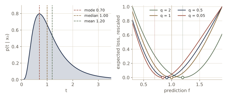
Choosing the loss when training
The same choice appears when we train, because each error function corresponds to a noise model. Minimizing the sum of squares is maximum likelihood under Gaussian noise, and the fitted model estimates the conditional mean. Minimizing the sum of absolute errors is maximum likelihood under Laplace noise, \(p(t \mid \mathbf{x}) \propto \exp(-\lvert t - y(\mathbf{x}, \mathbf{w}) \rvert / b)\), and the fitted model estimates the conditional median. When the real noise is skewed, the two fits differ, and each tracks its own target.
We fit both to 2000 points whose noise is skewed: \(t = h(x) + 0.5\,(e^{0.6 z} - 1)\) with \(z\) standard Gaussian, so the noise has median 0 but mean \(0.5\,(e^{0.18} - 1) \approx 0.099\). The conditional median is \(h(x)\) and the conditional mean is \(h(x) + 0.099\). The absolute-error fit uses iteratively reweighted least squares: a weighted least-squares problem, with weight \(1/\lvert r_n \rvert\) on a point whose current residual is \(r_n\), has the same stationarity condition as the absolute error, so we re-solve it until the weights stop changing.
def fit_abs(Phi, t, iters=100, floor=1e-6):
    """Minimize sum_n |t_n - w^T phi_n| by iteratively reweighted least squares."""
    w = fit_qr(Phi, t)
    for _ in range(iters):
        sw = 1 / np.sqrt(np.maximum(np.abs(t - forward(Phi, w)), floor))   # sqrt of the weights
        w = fit_qr(sw[:, None] * Phi, sw * t)
    return w

g = np.random.default_rng(12)
x_sk = g.uniform(-1, 1, 2000)
shift = 0.5 * (np.exp(S_LN**2 / 2) - 1)                   # mean of the noise
t_sk = h(x_sk) + 0.5 * (np.exp(S_LN * g.normal(size=2000)) - 1)
Phi_sk = design_matrix(x_sk, gauss_basis, MU, S)
Phi_g = design_matrix(x_grid, gauss_basis, MU, S)
fits = [("squared error ", fit_qr(Phi_sk, t_sk)), ("absolute error", fit_abs(Phi_sk, t_sk))]
for name, w_k in fits:
    y_g = forward(Phi_g, w_k)
    above = np.mean(t_sk > forward(Phi_sk, w_k))
    print(f"{name}: mean |y - E[t|x]| = {np.mean(np.abs(y_g - h(x_grid) - shift)):.4f}   "
          f"mean |y - median| = {np.mean(np.abs(y_g - h(x_grid))):.4f}   "
          f"targets above the fit: {above:.3f}")
squared error : mean |y - E[t|x]| = 0.0228   mean |y - median| = 0.0925   targets above the fit: 0.384
absolute error: mean |y - E[t|x]| = 0.1012   mean |y - median| = 0.0167   targets above the fit: 0.500
The squared-error fit tracks the conditional mean and leaves fewer than half of the targets above it; the absolute-error fit tracks the conditional median and splits the targets evenly, as its optimality condition requires. Neither is wrong: they answer different questions. When a single prediction is not enough, for instance when \(p(t \mid \mathbf{x})\) has several peaks, the right move is to model the whole conditional distribution, as the mixture density networks of module 06 do. The analogous decision theory for classification comes in module 05.
The bias–variance trade-off
The decomposition
We have seen that a flexible model fitted by maximum likelihood to a small data set overfits, that a regularizer controls it, and that minimizing the training error cannot choose the regularization coefficient. The bias–variance decomposition is a frequentist way to understand the trade-off behind that choice.
Write \(h(\mathbf{x}) = \mathbb{E}[t \mid \mathbf{x}]\) for the regression function. From the previous section, the expected squared loss of a predictor \(f\) is
\[\mathbb{E}[L] = \int \{f(\mathbf{x}) - h(\mathbf{x})\}^2 p(\mathbf{x})\, \mathrm{d}\mathbf{x} + \iint \{h(\mathbf{x}) - t\}^2 p(\mathbf{x}, t)\, \mathrm{d}\mathbf{x}\, \mathrm{d}t .\]The second term is noise. The first depends on the predictor, and the predictor depends on the training set \(\mathcal{D}\) we happened to draw, so write it \(f(\mathbf{x}; \mathcal{D})\). Imagine many independent training sets of the same size \(N\), all from \(p(\mathbf{x}, t)\), and average over them. At a fixed \(\mathbf{x}\), add and subtract the average prediction \(\mathbb{E}_{\mathcal{D}}[f(\mathbf{x}; \mathcal{D})]\):
\[\begin{aligned} \{f(\mathbf{x}; \mathcal{D}) - h(\mathbf{x})\}^2 &= \{f(\mathbf{x}; \mathcal{D}) - \mathbb{E}_{\mathcal{D}}[f(\mathbf{x}; \mathcal{D})]\}^2 + \{\mathbb{E}_{\mathcal{D}}[f(\mathbf{x}; \mathcal{D})] - h(\mathbf{x})\}^2 \\ &\quad + 2\{f(\mathbf{x}; \mathcal{D}) - \mathbb{E}_{\mathcal{D}}[f(\mathbf{x}; \mathcal{D})]\}\{\mathbb{E}_{\mathcal{D}}[f(\mathbf{x}; \mathcal{D})] - h(\mathbf{x})\} . \end{aligned}\]Averaged over \(\mathcal{D}\), the cross term vanishes, since its first factor averages to zero and its second does not depend on \(\mathcal{D}\):
\[\mathbb{E}_{\mathcal{D}}\left[\{f(\mathbf{x}; \mathcal{D}) - h(\mathbf{x})\}^2\right] = \underbrace{\{\mathbb{E}_{\mathcal{D}}[f(\mathbf{x}; \mathcal{D})] - h(\mathbf{x})\}^2}_{(\text{bias})^2} + \underbrace{\mathbb{E}_{\mathcal{D}}\left[\{f(\mathbf{x}; \mathcal{D}) - \mathbb{E}_{\mathcal{D}}[f(\mathbf{x}; \mathcal{D})]\}^2\right]}_{\text{variance}} .\]The squared bias is how far the average prediction, over all possible training sets, is from the truth. The variance is how much an individual prediction scatters around that average, that is, how sensitive the method is to the particular training set. Integrating over \(\mathbf{x}\):
Result. For squared loss, averaged over training sets of a fixed size,
\[\text{expected loss} = (\text{bias})^2 + \text{variance} + \text{noise},\]with \((\text{bias})^2 = \int \{\mathbb{E}_{\mathcal{D}}[f(\mathbf{x}; \mathcal{D})] - h(\mathbf{x})\}^2 p(\mathbf{x})\, \mathrm{d}\mathbf{x}\), \(\text{variance} = \int \mathbb{E}_{\mathcal{D}}[\{f(\mathbf{x}; \mathcal{D}) - \mathbb{E}_{\mathcal{D}}[f(\mathbf{x}; \mathcal{D})]\}^2]\, p(\mathbf{x})\, \mathrm{d}\mathbf{x}\), and \(\text{noise} = \iint \{h(\mathbf{x}) - t\}^2 p(\mathbf{x}, t)\, \mathrm{d}\mathbf{x}\, \mathrm{d}t\).
A rigid model (few basis functions, or a large \(\lambda\)) gives similar answers on every training set, so low variance, but may be unable to follow \(h\), so high bias. A flexible model can follow \(h\) on average but also follows each set’s noise: low bias, high variance. The best setting balances the two.
A simulation
We can run the thought experiment. Draw \(L = 200\) training sets of \(N = 25\) points from our \(h(x)\) with noise standard deviation 0.2. Fit each with a deliberately flexible model, 20 Gaussian bumps of width 0.1 plus a bias (\(M = 21\) parameters for 25 points), by ridge regression, for a range of \(\lambda\). With the fits \(f^{(l)}(x)\), the average prediction is \(\bar{f}(x) = \frac{1}{L} \sum_l f^{(l)}(x)\), and we replace the integrals over \(x\) by averages over 2000 test inputs \(x_i\) drawn from \(p(x)\):
\[(\text{bias})^2 \approx \frac{1}{N_{\text{test}}} \sum_{i} \{\bar{f}(x_i) - h(x_i)\}^2, \qquad \text{variance} \approx \frac{1}{N_{\text{test}}} \sum_{i} \frac{1}{L} \sum_{l} \{f^{(l)}(x_i) - \bar{f}(x_i)\}^2 .\]The noise is \(\sigma^2 = 0.04\) by construction. Separately, we measure what we would see in practice: the squared error of each fit on fresh noisy test targets, averaged over the test points and the 200 fits. If the decomposition is right, it should equal bias² + variance + noise.
MU20, S20 = np.linspace(-1, 1, 20), 0.1

def bias_variance(ln_lams, L=200, N=25, n_test=2000, seed=11):
    """Ridge fits to L training sets; returns rows (ln lambda, bias^2, variance, test error)."""
    g = np.random.default_rng(seed)
    sets = [make_data(N, g) for _ in range(L)]
    x_te = g.uniform(-1, 1, n_test)
    t_te = h(x_te) + g.normal(0, SIGMA, (L, n_test))     # fresh test targets for every fit
    Phi_te = design_matrix(x_te, gauss_basis, MU20, S20)
    Phis = [design_matrix(xl, gauss_basis, MU20, S20) for xl, _ in sets]
    rows = []
    for ln_lam in ln_lams:
        Y = np.array([forward(Phi_te, fit_ridge(P_l, t_l, np.exp(ln_lam)))
                      for P_l, (_, t_l) in zip(Phis, sets)])   # Y[l, i] = f^(l)(x_i)
        f_bar = Y.mean(axis=0)
        bias2 = np.mean((f_bar - h(x_te)) ** 2)
        variance = np.mean((Y - f_bar) ** 2)
        test = np.mean((Y - t_te) ** 2)
        rows.append((ln_lam, bias2, variance, test))
    return np.array(rows)

ln_lams = np.arange(-8, 4.01, 0.25)
bv = bias_variance(ln_lams)
noise = SIGMA**2
print(" ln lambda   bias^2   variance   + noise = sum   test error")
for ln_lam, b2, v, te in bv[::4]:
    print(f"{ln_lam:9.1f}   {b2:.4f}    {v:.4f}      {b2 + v + noise:.4f}       {te:.4f}")
i_sum, i_test = np.argmin(bv[:, 1] + bv[:, 2]), np.argmin(bv[:, 3])
print(f"minimum of bias^2 + variance at ln lambda = {bv[i_sum, 0]:.2f};"
      f" minimum test error at ln lambda = {bv[i_test, 0]:.2f}")
print(f"largest |test error - (bias^2 + variance + noise)|: "
      f"{np.max(np.abs(bv[:, 3] - bv[:, 1] - bv[:, 2] - noise)):.4f}")
 ln lambda   bias^2   variance   + noise = sum   test error
     -8.0   0.0053    0.5618      0.6072       0.6070
     -7.0   0.0032    0.2871      0.3303       0.3300
     -6.0   0.0019    0.1576      0.1994       0.1991
     -5.0   0.0012    0.0918      0.1329       0.1326
     -4.0   0.0009    0.0566      0.0976       0.0973
     -3.0   0.0011    0.0383      0.0794       0.0792
     -2.0   0.0021    0.0286      0.0707       0.0705
     -1.0   0.0055    0.0230      0.0686       0.0684
      0.0   0.0188    0.0193      0.0781       0.0780
      1.0   0.0641    0.0166      0.1207       0.1207
      2.0   0.1730    0.0133      0.2263       0.2263
      3.0   0.3274    0.0080      0.3755       0.3756
      4.0   0.4563    0.0032      0.4994       0.4995
minimum of bias^2 + variance at ln lambda = -1.25; minimum test error at ln lambda = -1.25
largest |test error - (bias^2 + variance + noise)|: 0.0003
The columns tell the story. At small \(\lambda\) the squared bias is tiny but the variance is large, because a 21-parameter model fitted to 25 points follows the noise of each training set. As \(\lambda\) grows the variance falls steadily. The squared bias is smallest near \(\ln \lambda = -4\) and then rises, slowly at first and then quickly, once the penalty flattens the fits so much that even their average misses \(h\). (Its small uptick at the far left is partly simulation noise: the average of 200 very erratic fits still carries about 1/200 of their variance.) Their sum has a minimum at a moderate \(\lambda\), and the measured test error has its minimum at the same place. Most importantly, the measured test error matches bias² + variance + noise to within a few ten-thousandths across the whole range; the only gap comes from the finite number of test targets.
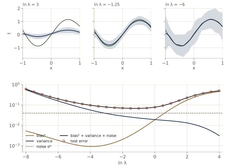
What the decomposition does and does not tell us
The decomposition is a way to think about model complexity rather than a way to choose it. It averages over an ensemble of training sets, and in practice we have one. If we really had 200 independent training sets, we would pool them into one large set, which would reduce overfitting far more than any choice of \(\lambda\). To choose \(\lambda\) from the data we have, we hold out data (validation and cross-validation, module 01), or we take a Bayesian route, in which averaging over the posterior distribution of the weights plays the role that averaging over data sets plays here (Intro to ML, module 03 develops it for this model).
Notice also the top panels of the figure: for small \(\lambda\), the individual fits are erratic, yet their average is close to \(h\). Averaging many high-variance, low-bias predictors reduces the variance and keeps the low bias, an idea that returns as model averaging and dropout in module 09.
Watch out. The tidy U-shaped curve is what we see when we vary a regularizer or a small number of basis functions in a linear model. Very large neural networks, with far more parameters than data points, can behave differently: the test error can fall again as the model grows past the point where it fits the training data exactly. Bishop & Bishop discuss this double descent in §9.3.2, and we meet it in module 09. The decomposition itself, an identity for squared loss, still holds; what changes is how bias and variance depend on model size.
Summary
| Idea | What it says | Key formula or property |
|---|---|---|
| Linear model as a network | fixed features, one layer of learned weights, one output node per target | \(y(\mathbf{x}, \mathbf{w}) = \mathbf{w}^{\mathrm{T}} \boldsymbol{\phi}(\mathbf{x})\), \(\mathbf{y} = \mathbf{W}^{\mathrm{T}} \boldsymbol{\phi}(\mathbf{x})\) |
| Maximum likelihood | Gaussian noise turns the likelihood into the sum-of-squares error | \(\mathbf{w}_{\mathrm{ML}} = \mathbf{\Phi}^{\dagger} \mathbf{t}\), \(\sigma^2_{\mathrm{ML}}\) = mean squared residual |
| Solvers | never invert; QR or SVD for accuracy, Cholesky when regularized | Cholesky on the normal equations squares \(\operatorname{cond}(\mathbf{\Phi})\) |
| Geometry | the fit is the projection of \(\mathbf{t}\) onto the column space | \(\mathbf{\Phi}^{\mathrm{T}}(\mathbf{t} - \mathbf{y}) = \mathbf{0}\), \(\mathbf{P} = \mathbf{Q}\mathbf{Q}^{\mathrm{T}}\) |
| SGD / LMS | per-example gradient steps reach the closed form with a decaying rate | \(\mathbf{w} \leftarrow \mathbf{w} + \eta (t_n - \mathbf{w}^{\mathrm{T}} \boldsymbol{\phi}_n) \boldsymbol{\phi}_n\); batch GD needs \(\eta < 2/\lambda_{\max}\) |
| Weight decay (ridge) | shrinks weights and fixes the conditioning | \((\lambda \mathbf{I} + \mathbf{\Phi}^{\mathrm{T}} \mathbf{\Phi})^{-1} \mathbf{\Phi}^{\mathrm{T}} \mathbf{t}\) |
| L1 penalty (lasso) | sets some weights exactly to zero | soft thresholding; proximal gradient descent |
| Decision theory | the loss picks the prediction from \(p(t \mid \mathbf{x})\) | squared: mean; absolute: median; window loss: mode |
| Bias–variance | expected loss splits into three parts | expected loss = bias² + variance + noise |
Ideas to carry forward:
- A network defines a conditional distribution, and its error function is the negative log likelihood. Change the noise model and you change both the error function and what the trained network estimates.
- Training by gradient descent is a loop of forward pass, error, gradient, and update. Even when a closed form exists, the loop converges only as fast as the conditioning of the error surface allows, and the learning rate must respect the steepest direction. These two facts shape everything in modules 07 and 08.
- The last layer of any deep regression network is exactly the model of this module, applied to learned features instead of hand-chosen ones.
- Model complexity is a trade-off between bias and variance, controlled here by \(\lambda\). Choosing it needs data or assumptions beyond the training error.
Exercises
- The flat direction of the running model came from the bias column and the sum of the bumps being nearly parallel. Compute \(\sum_j \phi_j(x)\) for the seven Gaussian bumps on a fine grid over \([-1, 1]\) and measure how far it is from constant, for widths \(s = 0.1, 0.25, 0.5\). Relate what you find to the smallest eigenvalue of \(\mathbf{\Phi}^{\mathrm{T}}\mathbf{\Phi}\) for each width, and predict (then check) how many SGD epochs the 3000-epoch experiment would need for each.
- Let \(\mathbf{P} = \mathbf{Q}\mathbf{Q}^{\mathrm{T}}\) be the projection onto the column space. Show that \(\mathbf{I} - \mathbf{P}\) is also a symmetric idempotent matrix, and that it projects onto the set of vectors orthogonal to every column. Use it to prove that the training error \(E_D(\mathbf{w}_{\mathrm{ML}})\) can never increase when a basis function is added to the model. Check this on the running data by adding the bumps of the 21-bump dictionary one at a time, and say why a falling training error is no evidence of a better model.
- When the noise level varies with the input, say \(\sigma(x) = 0.05 + 0.3\lvert x \rvert\), the likelihood gives each squared residual its own factor \(r_n = 1/\sigma(x_n)^2\). Derive the minimizer of \(\tfrac12 \sum_n r_n (t_n - \mathbf{w}^{\mathrm{T}} \boldsymbol{\phi}_n)^2\), and show that it is an ordinary least-squares problem after scaling row \(n\) of \(\mathbf{\Phi}\) and \(t_n\) by \(\sqrt{r_n}\) (the trick
fit_absuses). Over 200 simulated data sets of 30 points, compare the RMS error against \(h\) of the weighted and the unweighted fit. Which parts of the module still hold under this noise (the conditional mean as the best prediction, the bias–variance identity), and which formulas change? - For a model that contains the true function, \(\mathbf{t} = \mathbf{\Phi}\mathbf{w}_{\text{true}} + \boldsymbol{\epsilon}\) with \(\boldsymbol{\epsilon} \sim \mathcal{N}(\mathbf{0}, \sigma^2 \mathbf{I})\), show that \(\mathbb{E}[\sigma^2_{\mathrm{ML}}] = \frac{N - M}{N} \sigma^2\). (Hint: the residual is \((\mathbf{I} - \mathbf{P})\boldsymbol{\epsilon}\).) Check it by simulation with the running basis and targets generated from a fixed \(\mathbf{w}_{\text{true}}\).
- Batch gradient descent on the ridge error \(E_D(\mathbf{w}) + \tfrac{\lambda}{2}\mathbf{w}^{\mathrm{T}}\mathbf{w}\) multiplies the error along eigenvector \(\mathbf{u}_i\) of \(\mathbf{\Phi}^{\mathrm{T}}\mathbf{\Phi}\) by a fixed factor each step. Find the factor, the largest stable learning rate, and the number of steps needed to reduce the slowest component by a factor of \(e\), as functions of \(\lambda\). Evaluate your formula for the running model at \(\lambda = 0\) and \(\lambda = 0.1\) and compare with the SGD runs in the notes.
- Standardizing inputs is the simplest way to improve conditioning. Replace each non-bias column of the running design matrix by its version with zero mean and unit variance over the training set. Show that the least-squares fitted values do not change, compare the eigenvalues of \(\mathbf{\Phi}^{\mathrm{T}}\mathbf{\Phi}\) before and after, and rerun the 3000-epoch SGD experiment. How close does it get to the closed form now?
- Modify
trainto use mini-batches of size 1, 5, and 30 on the straight-line model, with the same number of gradient evaluations on single points for each. Plot the distance to the closed form against that count. Which batch size wins early on, and which at the end? Explain in terms of the noise in the gradient. - Implement coordinate descent for the L1-penalized error (update one weight at a time by soft thresholding its partial residual correlation). Check that it reaches the same weights as
fit_l1for the 21-bump model, and compare the number of passes each needs at \(\lambda = 0.1\). - For a continuous target, prove the median result without derivatives: show that for \(f < m\), where \(m\) is the conditional median, \(\mathbb{E}\lvert f - t \rvert - \mathbb{E}\lvert m - t \rvert \ge 0\). Then, for the log-normal example, find the minimizer of the expected pinball loss \(L = \max\{\alpha (t - f), (1 - \alpha)(f - t)\}\) for \(\alpha = 0.9\) numerically and identify it as a quantile.
- Redo the bias–variance simulation with the number of Gaussian bumps as the complexity knob instead of \(\lambda\): use \(M - 1 = 2, 4, \dots, 20\) bumps spread over \([-1, 1]\) (width equal to their spacing), a small fixed \(\lambda = 10^{-6}\), and plot bias², variance, and test error against \(M\). Where is the best \(M\), and how does the curve change for \(N = 100\)?
- Let \(p(t \mid \mathbf{x}_0)\) be an equal mixture of two Gaussians with means \(-1\) and \(1.5\) and standard deviations 0.3 and 0.5. Compute its mean, median, and mode, and the minimizers of the expected Minkowski loss for \(q = 2, 1, 0.5\) with
best_prediction(widen its search range). Which of these predictions would you ever want to report, and why does this example argue for modeling the whole conditional distribution instead of a single output? - In your own words: why can the same data set, the same model, and the same training data give different “best predictions” depending on the loss, and why does training with squared error make the network estimate the conditional mean? Explain it to a colleague who uses regression daily but has never thought about noise models.
Going further
- C. M. Bishop and H. Bishop, Deep Learning: Foundations and Concepts, chapter 4 — the source for this module. Exercises 4.1–4.2 (normal equations for polynomials), 4.3 (sigmoid and tanh), 4.4 (projection), 4.5 (weighted least squares), 4.6 (the regularized solution), 4.7 (general noise covariance), 4.8–4.10 (vector targets), and 4.11–4.12 (generalized Gaussian noise and Minkowski losses) extend the material here.
- Intro to ML, module 03 — the longer treatment of this model from Bishop’s Pattern Recognition and Machine Learning: conditioning of the normal equations, the lasso by coordinate descent, and the Bayesian treatment (posterior, predictive distribution, evidence) that sets \(\lambda\) from the training data alone.
- Gene H. Golub and Charles F. Van Loan, Matrix Computations (Johns Hopkins University Press) — the standard reference for QR, Cholesky, the SVD, and the numerical analysis of least squares.
- Trevor Hastie, Robert Tibshirani, and Jerome Friedman, The Elements of Statistical Learning (Springer, 2nd ed., 2009), free online — chapter 3 covers ridge, the lasso, and related shrinkage methods; chapter 7 covers the bias–variance trade-off and model selection.
- Within this course: module 06 makes the basis functions learnable, module 07 develops the optimizers whose difficulties we met here, and module 09 covers weight decay, early stopping, and double descent in deep networks.
These notes follow the chapters of C. M. Bishop and H. Bishop, Deep Learning: Foundations and Concepts (Springer, 2024), the course text, which the authors make free to read online. The explanations, code, figures, and exercises here are written for this course; the book remains the reference, with the full derivations and many more exercises.