CSE 676 · Module 01 · Week 1
The Deep Learning Revolution
What deep learning has changed, a first model fitted end to end (polynomial regression, overfitting, regularization, model selection), and a short history from the perceptron to deep networks.
Companion reading: Bishop & Bishop, Deep Learning: Foundations and Concepts, chapter 1, “The Deep Learning Revolution”
By the end of this module you can
- Tell supervised, unsupervised, and self-supervised learning apart, and classify a task as regression or classification, using the four applications in this module as examples.
- Fit polynomials of any order to data by least squares, starting from the normal equations, and check the solution numerically.
- Explain overfitting with the training and test root-mean-square errors, the size of the fitted coefficients, and the effect of more data.
- Derive the closed-form minimizer of the sum-of-squares error with a quadratic penalty and describe how the penalty weight controls effective complexity.
- Choose hyperparameters with a validation set and with S-fold cross-validation, and say what each costs and why a separate test set is still needed.
- Write a single artificial neuron as a weighted sum followed by an activation function, and show that the polynomial model is a special case.
- Run the perceptron algorithm, show that it cannot learn XOR, and show that one hidden layer fixes that.
- Outline the three phases of neural network history and name the developments behind the current one.
Contents
- The impact of deep learning
- A tutorial example
- A brief history of machine learning
- How this course is organized
- Summary
- Exercises
- Going further
This course is about deep learning: machine learning with neural networks that have many layers of adaptable parameters. Over the past decade and a half these models have gone from a research niche to the default tool for images, sound, text, molecules, and much else. The striking part is not any single result but the uniformity behind them. Problems that used to need separate specialist techniques are now attacked with variations of one framework: a large differentiable function, a data set, an error function, and gradient-based training.
This first module has three parts. We start with a tour of four applications, which also lets us set up the vocabulary used for the rest of the course. Then we work through a small regression problem from start to finish in NumPy: fitting a curve, watching it overfit, taming it with a penalty, and choosing its settings with held-out data. Every idea in that example returns later at a much larger scale. We finish with a short history of neural networks, from single artificial neurons to today’s deep networks.
If you took Intro to ML, the curve-fitting example will look familiar. Here we use different data and put the emphasis on what carries over to neural networks; the ML notes develop the probabilistic view of the same problem (likelihoods, priors, Bayesian curve fitting), which we return to in module 02.
The impact of deep learning
Bishop & Bishop §1.1 opens with four examples from quite different fields. We go through them briefly, because each one introduces a kind of learning problem we will meet again.
Medical diagnosis
Take photographs of skin lesions and ask whether each one is a malignant melanoma or a harmless mole. To the untrained eye the two classes can look almost the same, and nobody knows how to write down rules that separate them reliably. What we can do is collect many images, each with a label confirmed by a biopsy, and let a network with millions of adjustable weights find a mapping from image to label. Setting the weights from data is called learning or training, and the labeled images form the training set.
This is supervised learning: every training input comes with the answer we want the model to produce. It is also classification, because the output is one of a discrete set of classes (malignant or benign). When the output is one or more continuous quantities instead, such as the yield of a chemical process as a function of temperature and pressure, the task is regression.
One detail of the published skin-lesion work (Esteva et al., 2017) matters for this course. The labeled medical images were not numerous by deep learning standards, so the network was first trained on a large, general collection of everyday photographs and only then adjusted on the lesion images. Reusing what a network learned on one task to help with another is transfer learning. The first stage teaches general facts about natural images (edges, textures, shapes); the second specializes them.
Protein structure
A protein is a chain of amino acids that folds into a three-dimensional shape, and that shape largely determines what the protein does. Reading the sequence of a protein is comparatively cheap; measuring its 3-D structure with experimental methods such as X-ray crystallography or cryo-electron microscopy is slow and sometimes fails. Predicting structure from sequence was a central open problem in biology for decades.
Deep learning changed that. A network trained on proteins whose sequence and structure are both known can take a new sequence and output a predicted structure (Jumper et al., 2021, describe the AlphaFold system). The input here is a sequence and the output a geometric object, but the setting is again supervised learning: inputs paired with known answers.
Image synthesis
Now drop the labels. Suppose the training data are just a large set of photographs of faces, and the goal is to produce new faces that look like they came from the same collection without copying any of them. Learning from unlabeled data is unsupervised learning, and a model that can produce new examples with the same statistical character as its training data is a generative model. Modern generative models produce images that are hard to tell from photographs.
A variant conditions the output on a piece of text, the prompt, so that the image reflects what the text describes. The umbrella term generative AI covers models that generate images, video, audio, text, molecules, or other kinds of data. The later part of this course (modules 17–20) is about how such models are built.
Large language models
A large language model (LLM) is a network trained on a very large amount of text. The most common kind is autoregressive: given a sequence of words (more precisely, tokens, which may be words or pieces of words), it predicts the next one. To produce a passage, we append the predicted token to the input and run the model again, token after token, until it emits a special end-of-text token. A conversation works the same way: the user’s reply is appended to the sequence and generation continues.
Where do the training labels come from? From the text itself: every position in every document supplies an input (the tokens so far) and a target (the token that actually comes next). Supervised-style training with labels extracted automatically from unlabeled data is self-supervised learning. Because text is abundant, this scales to enormous data sets and correspondingly large networks, and the resulting models can answer questions, write code, and carry out many tasks they were never explicitly trained for. We build the architecture behind them, the transformer, in module 12.
| Example | Input | Output | Kind of learning |
|---|---|---|---|
| Skin lesions | image | class (malignant / benign) | supervised classification, with transfer learning |
| Protein structure | amino acid sequence | 3-D structure | supervised, structured output |
| Image synthesis | none, or a text prompt | a new image | unsupervised generative modeling |
| Language models | tokens so far | the next token | self-supervised, generative |
Note. These four problems look unrelated, but all four were solved with the same ingredients: a neural network with many adjustable weights, an error function that measures how wrong its outputs are, and gradient-based training on a large data set. The rest of the course takes those ingredients apart one at a time.
A tutorial example
The big applications are too large to study in detail on day one. A tiny regression problem shows almost every basic concept at once: a model with parameters, an error function, fitting, generalization, overfitting, regularization, and choosing settings from data (Bishop & Bishop §1.2).
Synthetic data
We observe a real-valued input \(x\) and a real-valued target \(t\). The training set consists of \(N\) input values \(x_1, \dots, x_N\) with their targets \(t_1, \dots, t_N\), and the task is to predict \(t\) at new values of \(x\). Doing well on inputs the model has not seen is called generalization, and it is the whole point: fitting the training points is easy, predicting new ones is not.
We generate the data ourselves so that we know the truth. The hidden function is
\[f(x) = 0.6\cos(4x) + 0.4\,x, \qquad -1 \le x \le 1,\]a gentle wave on a slight slope. Each target is \(t_n = f(x_n) + \epsilon_n\) with Gaussian noise \(\epsilon_n\) of standard deviation \(\sigma = 0.2\). The noise stands for everything that makes real measurements scatter around a regular trend: sources of variability we do not observe. For the training set we take \(N = 12\) inputs spread over \([-1, 1]\) by placing one uniformly random point in each of 12 equal subintervals, so the whole range is covered but the spacing is irregular. A test set of 1000 points with uniformly random inputs comes from the same source; we use it only to measure generalization.
import numpy as np

np.set_printoptions(precision=4, suppress=True)
rng = np.random.default_rng(676)

SIGMA = 0.2                                  # noise standard deviation

def f_true(x):
    """The hidden trend that generates the targets."""
    return 0.6 * np.cos(4 * x) + 0.4 * x

def make_data(N, rng, stratified=True):
    """N pairs (x_n, t_n) with t_n = f(x_n) + Gaussian noise, x in [-1, 1].
    stratified: one uniform point in each of N equal subintervals; else uniform."""
    if stratified:
        x = -1 + 2 * (np.arange(N) + rng.uniform(0, 1, N)) / N
    else:
        x = rng.uniform(-1, 1, N)
    t = f_true(x) + rng.normal(0, SIGMA, N)
    return x, t

x, t = make_data(12, rng)                              # training set
x_test, t_test = make_data(1000, rng, stratified=False)  # test set
print("x =", x)
print("t =", t)
x = [-0.9551 -0.751  -0.6585 -0.3959 -0.1965 -0.042   0.1532  0.1918  0.476
  0.6172  0.7154  0.8743]
t = [-0.9284 -1.1064 -0.7114 -0.2297  0.2788  0.8276  0.3564  0.2183  0.0888
 -0.0088 -0.3206 -0.4911]
Linear models
As our model we use a polynomial of order \(M\),
\[y(x, \mathbf{w}) = w_0 + w_1 x + w_2 x^2 + \dots + w_M x^M = \sum_{j=0}^{M} w_j x^j ,\]with coefficients \(\mathbf{w} = (w_0, \dots, w_M)^{\mathrm{T}}\). The polynomial is nonlinear in \(x\) but linear in \(\mathbf{w}\). Models that are linear in their unknown parameters are called linear models. That linearity is what makes this example solvable in closed form. It is also their main limitation: the functions \(x^j\) are fixed before we see any data, and a neural network’s main departure from a linear model is to learn such functions instead (module 04 treats linear models as single-layer networks; module 06 makes the basis functions adaptive).
It helps to write all predictions at once. Collect the powers of the inputs in the \(N \times (M+1)\) design matrix \(\boldsymbol{\Phi}\), with entries \(\Phi_{nj} = x_n^j\). Then the vector of predictions at the training inputs is \(\boldsymbol{\Phi}\mathbf{w}\).
Error function
To fit the model we need a number that says how badly a given \(\mathbf{w}\) fits the training data. The standard choice for regression is the sum-of-squares error function
\[E(\mathbf{w}) = \frac{1}{2}\sum_{n=1}^{N} \bigl( y(x_n, \mathbf{w}) - t_n \bigr)^2 = \frac{1}{2}\lVert \boldsymbol{\Phi}\mathbf{w} - \mathbf{t} \rVert^2 ,\]where \(\mathbf{t} = (t_1, \dots, t_N)^{\mathrm{T}}\). It is never negative, and it is zero exactly when the curve passes through every training point. The factor \(\tfrac12\) only tidies the derivative. In module 02 we will see that this error is not an arbitrary choice: it is what maximum likelihood gives when the noise is Gaussian.
Because \(E\) is quadratic in \(\mathbf{w}\), its gradient is linear in \(\mathbf{w}\), and setting the gradient to zero gives a linear system. Expanding the squared norm and differentiating,
\[\nabla E(\mathbf{w}) = \boldsymbol{\Phi}^{\mathrm{T}}(\boldsymbol{\Phi}\mathbf{w} - \mathbf{t}) = \mathbf{0} \quad\Longrightarrow\quad \boldsymbol{\Phi}^{\mathrm{T}}\boldsymbol{\Phi}\,\mathbf{w}^{\star} = \boldsymbol{\Phi}^{\mathrm{T}}\mathbf{t}.\]These are the normal equations. When the columns of \(\boldsymbol{\Phi}\) are linearly independent (here: at least \(M+1\) distinct inputs), \(\boldsymbol{\Phi}^{\mathrm{T}}\boldsymbol{\Phi}\) is positive definite, so \(E\) is strictly convex and \(\mathbf{w}^{\star}\) is its unique minimizer. In code we let np.linalg.lstsq solve the least-squares problem directly (it works from an SVD of \(\boldsymbol{\Phi}\), which is numerically safer than forming \(\boldsymbol{\Phi}^{\mathrm{T}}\boldsymbol{\Phi}\)) and check it against the normal equations.
To compare errors across data sets of different sizes, and in the same units as \(t\), we report the root-mean-square error
\[E_{\mathrm{RMS}} = \sqrt{\frac{1}{N}\sum_{n=1}^{N} \bigl( y(x_n, \mathbf{w}) - t_n \bigr)^2 } .\]def design_matrix(x, M):
"""Phi[n, j] = x_n ** j, j = 0..M; shape (N, M + 1)."""
return x[:, None] ** np.arange(M + 1)
def fit_poly(x, t, M, lam=0.0):
"""w minimizing E(w) + (lam / 2) ||w||^2 for an order-M polynomial."""
Phi = design_matrix(x, M)
if lam == 0.0:
return np.linalg.lstsq(Phi, t, rcond=None)[0] # plain least squares
A = Phi.T @ Phi + lam * np.eye(M + 1) # regularized normal eqs.
return np.linalg.solve(A, Phi.T @ t)
def predict(w, x):
"""y(x, w) at every entry of x."""
return design_matrix(x, len(w) - 1) @ w
def rms(w, x, t):
"""E_RMS: square root of the mean squared residual."""
return np.sqrt(np.mean((predict(w, x) - t) ** 2))
# check on M = 4: lstsq solves the normal equations, and the gradient vanishes there
Phi = design_matrix(x, 4)
w4 = fit_poly(x, t, 4)
w4_normal = np.linalg.solve(Phi.T @ Phi, Phi.T @ t)
print("w* (M = 4):", w4)
print(f"largest difference from normal equations: {np.abs(w4 - w4_normal).max():.1e}")
print(f"size of the gradient at w*: {np.linalg.norm(Phi.T @ (Phi @ w4 - t)):.1e}")
w* (M = 4): [ 0.4978  0.5283 -3.3157 -0.2375  2.2226]
largest difference from normal equations: 3.4e-14
size of the gradient at w*: 4.2e-15
Both routes give the same coefficients, and the gradient at the solution is zero up to rounding error. Fitting is solved; the hard question is which order \(M\) to use.
Model complexity
Choosing \(M\) is our first example of model selection. Let us fit every order from 0 up to 11 (twelve coefficients for twelve points) and record the error on the training set and on the test set, together with the largest coefficient.
print(" M   train E_RMS   test E_RMS   max |w_j|")
for M in range(12):
    w = fit_poly(x, t, M)
    print(f"{M:2d}   {rms(w, x, t):11.4f}   {rms(w, x_test, t_test):10.4f}   "
          f"{np.abs(w).max():9.1f}")
 M   train E_RMS   test E_RMS   max |w_j|
 0        0.5471       0.5284         0.2
 1        0.4921       0.4758         0.4
 2        0.2358       0.2910         1.5
 3        0.2212       0.3036         1.5
 4        0.1535       0.2104         3.3
 5        0.1376       0.2385         3.1
 6        0.1334       0.2591         5.6
 7        0.1293       0.2248        12.7
 8        0.0568       0.7287       111.1
 9        0.0568       0.7243       110.8
10        0.0062       1.1656       616.4
11        0.0000       1.2970       862.9
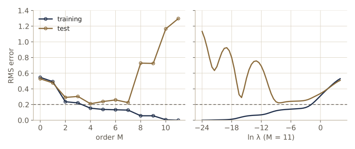
Read the table from the top. Orders 0 and 1 (a constant and a line) cannot bend, so both errors are large. From \(M = 2\) the fit starts to follow the wave, and \(M = 4\) has the smallest test error, about 0.21. That is close to the noise level \(\sigma = 0.2\), which is the best any predictor could achieve on average: even the true \(f\) would have test \(E_{\mathrm{RMS}}\) near 0.2, because the noise itself cannot be predicted. From \(M = 8\) on, the training error drops sharply and reaches zero at \(M = 11\), where the polynomial has as many coefficients as there are points and can pass through all of them. The test error, meanwhile, rises to about six times its best value. This is overfitting: the model has tuned itself to the particular noise in the training targets rather than to the trend behind them.
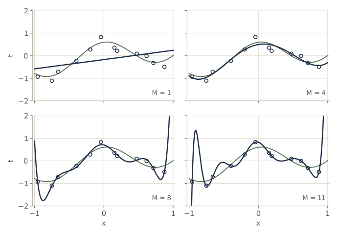
At first this looks paradoxical. Every polynomial of order 4 is also a polynomial of order 11 (with the last seven coefficients zero), so the larger family can do at least as well. The catch is that least squares does not pick the member of the family that generalizes best; it picks the one that fits the twelve given points best, and with enough freedom that means fitting the noise. The last column of the table shows how: the largest coefficient grows from a few units at \(M = 4\) to hundreds at \(M = 11\). Large coefficients of opposite signs cancel almost exactly at the data points and produce big swings between them. Here are the two sets side by side.
for M in [4, 11]:
    print(f"M = {M:2d}:", fit_poly(x, t, M))
M =  4: [ 0.4978  0.5283 -3.3157 -0.2375  2.2226]
M = 11: [   0.8223   -1.0099  -20.117    28.2344  147.2533 -207.1346 -441.2618
  642.2889  548.0814 -862.9029 -234.8269  411.3657]
How much a given order overfits depends on how much data we have. Holding \(M = 11\) fixed and increasing \(N\), the same model class becomes harmless, because the noise on many points averages out and there is no longer enough freedom to chase each one.
for N in [12, 24, 48, 192]:
    xN, tN = make_data(N, np.random.default_rng(N))
    wN = fit_poly(xN, tN, 11)
    print(f"N = {N:3d}:  train E_RMS = {rms(wN, xN, tN):.4f}   "
          f"test E_RMS = {rms(wN, x_test, t_test):.4f}   "
          f"max |w_j| = {np.abs(wN).max():7.1f}")
N =  12:  train E_RMS = 0.0000   test E_RMS = 5.2203   max |w_j| =  2463.2
N =  24:  train E_RMS = 0.1302   test E_RMS = 0.3231   max |w_j| =   411.7
N =  48:  train E_RMS = 0.1600   test E_RMS = 0.2176   max |w_j| =   223.6
N = 192:  train E_RMS = 0.1867   test E_RMS = 0.2004   max |w_j| =    36.5
Each row is a fresh data set. With 192 points the order-11 polynomial generalizes about as well as the order-4 one did on 12 points. A rule of thumb from classical statistics follows: have several times (say 5 to 10 times) as many data points as parameters.
That rule is worth measuring against a network of the kind used later in the course. A fully connected network for 28 × 28 digit images, with two hidden layers of 256 units and 10 outputs, has these many parameters:
layers = [784, 256, 256, 10]
n_params = sum(d_in * d_out + d_out for d_in, d_out in zip(layers[:-1], layers[1:]))
print(f"parameters: {n_params:,}")
print(f"parameters per image, 60,000 training images: {n_params / 60000:.1f}")
parameters: 269,322
parameters per image, 60,000 training images: 4.5
That is several parameters per training image, the opposite of the classical rule, and yet such networks generalize well on digit data. Deep learning routinely works in this regime, with far more parameters than training points. The reasons are subtle (the architecture, the way training proceeds, and implicit regularization all play a part), and module 09 returns to them. For now, keep in mind that counting parameters is a poor measure of how complex a model effectively is.
Watch out. The training error cannot tell you which model generalizes. It only ever decreases as the model family grows, so choosing the model with the lowest training error always selects the most flexible one. Every decision about model complexity must be made with data the model was not fitted to.
Regularization
Limiting the number of parameters according to the amount of data is unsatisfying: the complexity of the model should reflect the complexity of the problem, not the size of the sample we happen to have. A different approach keeps the flexible model and adds a penalty that discourages large coefficients. Regularization replaces the error function by
\[\widetilde{E}(\mathbf{w}) = \frac{1}{2}\sum_{n=1}^{N}\bigl( y(x_n, \mathbf{w}) - t_n \bigr)^2 + \frac{\lambda}{2}\lVert \mathbf{w} \rVert^2 ,\]where \(\lVert \mathbf{w} \rVert^2 = \mathbf{w}^{\mathrm{T}}\mathbf{w} = w_0^2 + \dots + w_M^2\) and \(\lambda \ge 0\) sets how strongly the penalty counts against the data fit. In statistics this is a shrinkage method (for this particular penalty, ridge regression); in neural networks the same quadratic penalty is called weight decay, because it pulls every weight toward zero.
The penalized error is still quadratic, so we can minimize it exactly. The penalty adds \(\lambda\mathbf{w}\) to the gradient:
\[\nabla\widetilde{E}(\mathbf{w}) = \boldsymbol{\Phi}^{\mathrm{T}}(\boldsymbol{\Phi}\mathbf{w} - \mathbf{t}) + \lambda\mathbf{w} = \mathbf{0} \quad\Longrightarrow\quad \mathbf{w}^{\star}_{\lambda} = \bigl(\lambda\mathbf{I} + \boldsymbol{\Phi}^{\mathrm{T}}\boldsymbol{\Phi}\bigr)^{-1}\boldsymbol{\Phi}^{\mathrm{T}}\mathbf{t}.\]For any \(\lambda > 0\) the matrix \(\lambda\mathbf{I} + \boldsymbol{\Phi}^{\mathrm{T}}\boldsymbol{\Phi}\) is positive definite, so the solution is unique even when there are more coefficients than data points. That is the lam > 0 branch of fit_poly, which solves the system with np.linalg.solve rather than forming the inverse. We penalize all coefficients, including \(w_0\), to match the formula; in practice \(w_0\) is often left out of the penalty (or given its own weight), since penalizing it makes the fit depend on where the origin of \(t\) is.
Now sweep \(\lambda\) for the order-11 polynomial. Because useful values span many orders of magnitude, we step through \(\ln\lambda\).
print("  ln lam   train E_RMS   test E_RMS   ||w||")
for ln_lam in [-20, -15, -10, -7, -5, -3, -1, 1]:
    w = fit_poly(x, t, 11, np.exp(ln_lam))
    print(f"{ln_lam:8d}   {rms(w, x, t):11.4f}   {rms(w, x_test, t_test):10.4f}   "
          f"{np.linalg.norm(w):7.2f}")
  ln lam   train E_RMS   test E_RMS   ||w||
     -20        0.0055       0.8650    839.72
     -15        0.0532       0.5353    181.56
     -10        0.1024       0.3393     30.44
      -7        0.1374       0.2350      4.53
      -5        0.1456       0.2434      2.64
      -3        0.1620       0.2548      2.03
      -1        0.2484       0.3087      1.11
       1        0.3734       0.3804      0.45
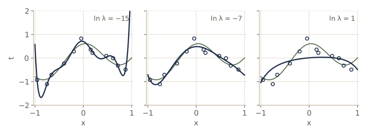
A very small \(\lambda\) (the first row) leaves the fit nearly as wild as with no penalty at all. As \(\lambda\) grows the coefficient norm shrinks by orders of magnitude, the training error rises, and the test error falls; around \(\ln\lambda = -7\) the order-11 polynomial generalizes about as well as the best unregularized order did (0.235 against 0.210). A large \(\lambda\) then flattens the curve too much and both errors climb. The penalty weight therefore acts as a dial on the effective complexity of the model, even though the number of parameters never changes.
Note. Regularization appears throughout deep learning in many forms: weight decay, early stopping, dropout, data augmentation, and architectural constraints. All of them trade a little fit to the training data for better behavior on new data. Module 09 covers them; for the Bayesian reading of the quadratic penalty as a Gaussian prior on the weights, see Intro to ML, module 01.
Model selection
The order \(M\) and the penalty weight \(\lambda\) are hyperparameters: they are fixed while we minimize the error over \(\mathbf{w}\). We cannot fit them by minimizing the same error jointly with \(\mathbf{w}\), because that drives \(\lambda \to 0\) and \(M\) to its maximum, which is exactly the overfitted model. So far we cheated by peeking at the test set. In practice we have only the data we collected, and we need a way to choose hyperparameters from it.
The simplest way is to split the available data. Fit \(\mathbf{w}\) on a training set, compare the candidate hyperparameter settings on held-back data, the validation set (other names: hold-out set, development set), and keep the best. If we try many settings, we slowly overfit the validation set as well, so the final performance should be measured once on a third, untouched test set.
Suppose we have collected 30 points. We shuffle them, fit on 20, and validate on 10.
x_pool, t_pool = make_data(30, rng)                 # all the data we have
perm = rng.permutation(30)
tr, va = perm[:20], perm[20:]

val_err = []
for M in range(12):
    w = fit_poly(x_pool[tr], t_pool[tr], M)
    val_err.append(rms(w, x_pool[va], t_pool[va]))
M_best = int(np.argmin(val_err))
print("validation E_RMS, M = 0..5: ", np.round(val_err[:6], 3))
print("validation E_RMS, M = 6..11:", np.round(val_err[6:], 3))
w_final = fit_poly(x_pool, t_pool, M_best)          # refit on all 30 points
print(f"chosen M = {M_best};  test E_RMS of the refit = "
      f"{rms(w_final, x_test, t_test):.4f}")
validation E_RMS, M = 0..5:  [0.367 0.31  0.317 0.352 0.223 0.216]
validation E_RMS, M = 6..11: [0.217 0.268 0.299 0.232 0.232 0.706]
chosen M = 5;  test E_RMS of the refit = 0.2177
The validation errors follow the earlier test-error curve only roughly (orders 9 and 10 score almost as well as orders 4 to 6), but the order they pick, \(M = 5\), generalizes well: its test error is 0.218. Notice that the final model is refitted on all 30 points once \(M\) is chosen: the split was only a device for choosing.
A 10-point validation set is small, and its error is a noisy estimate; a different random split might pick a different \(M\). S-fold cross-validation reduces that noise without giving up training data. Divide the data into \(S\) groups (folds) of nearly equal size. For each fold in turn, train on the other \(S - 1\) folds and measure the error on the held-out one. Every point is used for validation exactly once, and each model is trained on a fraction \((S-1)/S\) of the data. With \(S = N\) each fold is a single point, and the method is called leave-one-out cross-validation. (The same idea is often called K-fold cross-validation; we keep \(K\) for the number of classes.)
def folds(N, S, rng):
    """A random partition of 0..N-1 into S folds of nearly equal size."""
    return np.array_split(rng.permutation(N), S)

def cv_rms(x, t, M, lam=0.0, S=5, seed=0):
    """S-fold cross-validation estimate of E_RMS for order M and penalty lam."""
    sq = 0.0
    for hold in folds(len(x), S, np.random.default_rng(seed)):   # same folds each call
        keep = np.setdiff1d(np.arange(len(x)), hold)
        w = fit_poly(x[keep], t[keep], M, lam)
        sq += np.sum((predict(w, x[hold]) - t[hold]) ** 2)
    return np.sqrt(sq / len(x))

cv5 = [cv_rms(x_pool, t_pool, M) for M in range(12)]
loo = [cv_rms(x_pool, t_pool, M, S=30) for M in range(12)]
print(" M   5-fold CV   leave-one-out")
for M in range(12):
    print(f"{M:2d}   {cv5[M]:9.3f}   {loo[M]:13.3f}")
print(f"5-fold picks M = {np.argmin(cv5)}, leave-one-out picks M = {np.argmin(loo)}")
 M   5-fold CV   leave-one-out
 0       0.459           0.460
 1       0.425           0.434
 2       0.315           0.305
 3       0.306           0.317
 4       0.224           0.230
 5       0.273           0.240
 6       0.296           0.271
 7       0.379           0.309
 8       0.441           0.422
 9       0.532           0.315
10       0.641           0.572
11       1.259           1.259
5-fold picks M = 4, leave-one-out picks M = 4
Both estimates pick \(M = 4\), and both follow the shape of the test-error curve from the previous section: high for the stiff models, lowest around \(M = 4\), and rising steeply for the largest orders. Neither drops much below 0.22, as expected with noise of standard deviation 0.2. Seeding the fold generator inside cv_rms means every candidate is evaluated on the same folds, so differences between candidates come from the models, not from different random splits.
Cross-validation can choose several hyperparameters at once by searching a grid. Here we choose \(M\) and \(\ln\lambda\) together and count the fits it costs.
orders = range(3, 12)
ln_lams = np.arange(-16, 1, 2.0)
scores = np.array([[cv_rms(x_pool, t_pool, M, np.exp(a)) for a in ln_lams]
                   for M in orders])
i, j = np.unravel_index(np.argmin(scores), scores.shape)
M_cv, ln_cv = list(orders)[i], ln_lams[j]
w_cv = fit_poly(x_pool, t_pool, M_cv, np.exp(ln_cv))
print(f"grid: {len(orders)} orders x {len(ln_lams)} penalties x 5 folds "
      f"= {scores.size * 5} fits")
print(f"best: M = {M_cv}, ln lam = {ln_cv:.0f}, CV E_RMS = {scores[i, j]:.4f}")
print(f"test E_RMS of the refit on all 30 points: {rms(w_cv, x_test, t_test):.4f}")
grid: 9 orders x 9 penalties x 5 folds = 405 fits
best: M = 4, ln lam = -4, CV E_RMS = 0.2162
test E_RMS of the refit on all 30 points: 0.2235
The selected combination does about as well on the test set as the order chosen by the simple validation split. What the grid makes plain is the cost. Cross-validation multiplies the number of training runs by \(S\), and a grid over several hyperparameters grows exponentially with their number. For a polynomial each fit takes microseconds. For a large neural network each fit can take days on many GPUs, so exhaustive searches are out of the question and practitioners lean on experience from smaller models, sensible defaults, and a few well-chosen runs.
In practice. Keep three roles for data separate: training data fit the weights, validation data (or cross-validation) choose hyperparameters and architectures, and a test set that played no part in any decision reports the final performance. Report the test number once, at the end.
From the tutorial example to deep learning
The toy problem has the same skeleton as the applications in the first section: a parametric function, an error function, minimization over the parameters, and held-out data to check generalization. Real problems differ in scale and in one essential way. Data sets can be many orders of magnitude larger; inputs can have thousands or millions of dimensions (every pixel of an image) and outputs many components. The function is a neural network with a very large number of weights, and the error is a highly nonlinear function of them, so there is no closed-form minimizer. Instead we compute the gradient of the error with respect to every weight and take many small steps downhill, which is the subject of module 07 (optimization) and module 08 (computing the gradient).
A brief history of machine learning
Over the decades the field has explored many approaches. Following Bishop & Bishop §1.3, we trace only the line that leads to deep learning: neural networks.
The original inspiration came from the brain. Its basic processing cells, neurons, are electrically active. When a neuron fires, an electrical pulse travels along its axon to junctions called synapses, where chemical signals pass to other neurons and make them more likely (an excitatory synapse) or less likely (an inhibitory synapse) to fire. A human brain has on the order of a hundred billion neurons, each with thousands of synapses, and changes in the strengths of synapses are a key mechanism by which it learns.
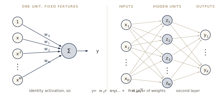
Simple mathematical models of this behavior go back to McCulloch and Pitts (1943). The model that the rest of this course builds on describes one artificial neuron in two steps: take a weighted sum of the inputs, then pass it through a nonlinear function,
\[a = \sum_{i=1}^{D} w_i x_i, \qquad y = f(a).\]The inputs \(x_1, \dots, x_D\) play the role of the activities of other neurons, the weights \(w_i\) the synapse strengths, \(a\) is the pre-activation, \(f\) the activation function, and \(y\) the activation or output. Our polynomial is a special case: take the inputs to be the powers \(x_i = x^i\) of a single variable (with \(x^0 = 1\) supplying \(w_0\)) and let \(f\) be the identity. So the tutorial example was already a one-neuron network with hand-chosen input features.
The history of neural networks falls roughly into three phases, distinguished by how many layers of weights could be trained.
Single-layer networks
The best-known early model is Rosenblatt’s perceptron, developed from the late 1950s. Its activation function is a step,
\[f(a) = \begin{cases} 0, & a \le 0, \\ 1, & a > 0, \end{cases}\]so the unit fires only when the weighted input exceeds a threshold. Rosenblatt gave a learning rule that adjusts the weights after each misclassified example, and it comes with a guarantee: if some weight vector classifies every training point correctly, the algorithm finds one in a finite number of steps. The perceptron was also built as dedicated hardware, with a camera-like array of photocells for input and motor-driven potentiometers as adjustable weights. It had several stages of processing but only one layer of learnable weights, which is why it counts as a single-layer network.
The perceptron rule is short enough to write now. With targets coded as \(t_n \in \{-1, +1\}\) and a bias handled by a constant input \(x_0 = 1\), each misclassified point (one with \(t_n \mathbf{w}^{\mathrm{T}}\mathbf{x}_n \le 0\)) triggers the update \(\mathbf{w} \leftarrow \mathbf{w} + t_n\mathbf{x}_n\), which moves \(\mathbf{w}^{\mathrm{T}}\mathbf{x}_n\) toward the correct sign. We run it on two separable clouds of points and then on the four points of the exclusive-or (XOR) problem, where the class is 1 when exactly one of two binary inputs is 1.
def perceptron(X, t, max_epochs=100):
    """Rosenblatt's rule for targets t in {-1, +1}; X has a leading column of ones.
    Returns the weights and the number of mistakes in each pass through the data."""
    w = np.zeros(X.shape[1])
    mistakes = []
    for epoch in range(max_epochs):
        m = 0
        for x_n, t_n in zip(X, t):
            if t_n * (w @ x_n) <= 0:           # misclassified (or on the boundary)
                w = w + t_n * x_n
                m += 1
        mistakes.append(m)
        if m == 0:                             # a clean pass: all points correct
            break
    return w, mistakes

def add_bias(X):
    return np.hstack([np.ones((len(X), 1)), X])

# two separable clouds of 40 points each
X2 = np.vstack([rng.normal([-1.0, -0.5], 0.5, (40, 2)),
                rng.normal([1.0, 0.5], 0.5, (40, 2))])
t2 = np.repeat([-1, 1], 40)
w_sep, m_sep = perceptron(add_bias(X2), t2)
print(f"separable clouds: mistakes per pass {m_sep}, final w = {w_sep}")

# XOR
X_xor = np.array([[0, 0], [0, 1], [1, 0], [1, 1]], dtype=float)
t_xor = np.array([-1, 1, 1, -1])
w_xor, m_xor = perceptron(add_bias(X_xor), t_xor)
print(f"XOR: {len(m_xor)} passes, mistakes in the last five: {m_xor[-5:]}, "
      f"final w = {w_xor}")
separable clouds: mistakes per pass [2, 2, 1, 0], final w = [-1.      1.9448  0.6079]
XOR: 100 passes, mistakes in the last five: [4, 4, 4, 4, 4], final w = [0. 0. 0.]
On the separable clouds the number of mistakes falls to zero within a few passes, and the rule stops. On XOR every pass makes four mistakes and the weights return to zero by the end of it, so the rule cycles forever. No amount of training could help: a single unit separates its inputs with a straight line, and no line puts \((0,1)\) and \((1,0)\) on one side and \((0,0)\) and \((1,1)\) on the other. Minsky and Papert’s book Perceptrons (1969) analyzed such limitations of single-layer networks rigorously. They also suggested that networks with several learnable layers might be no better, a conjecture that later proved wrong. Together with the lack of any algorithm for training more than one layer, this dampened interest and funding in neural networks through the 1970s. The name survives: a modern fully connected network is still often called a multilayer perceptron (MLP).
Backpropagation
Two changes opened the way to networks with several layers of learnable weights. The step function was replaced by smooth activation functions with nonzero derivatives, and the training goal was expressed as a differentiable error function, like the sum-of-squares error of the tutorial example. With both changes in place, every weight in the network has a well-defined error derivative that can be computed.
In a network with more than one layer, the units in the middle are hidden units: the training data give values for the inputs and the targets, but never for them. Each hidden and output unit computes a weighted sum followed by an activation function, and a network whose connections all point from inputs toward outputs, with no loops, is a feed-forward network. What a hidden layer buys is easiest to see on XOR. Two hidden units with hand-set weights, one computing OR and one computing AND, give a representation in which XOR is linearly separable: XOR is “OR but not AND”.
step = lambda a: (a > 0).astype(float)

W1 = np.array([[1.0, 1.0],       # hidden unit 1: OR,  fires if x1 + x2 > 0.5
               [1.0, 1.0]])      # hidden unit 2: AND, fires if x1 + x2 > 1.5
b1 = np.array([-0.5, -1.5])
w2, b2 = np.array([1.0, -2.0]), -0.5      # output: fires if OR - 2 AND > 0.5

Z = step(X_xor @ W1.T + b1)               # hidden activations z_j = h(a_j)
y = step(Z @ w2 + b2)
for x_n, z_n, y_n in zip(X_xor, Z, y):
    print(f"x = {x_n}   hidden z = {z_n}   output y = {y_n:.0f}")
x = [0. 0.]   hidden z = [0. 0.]   output y = 0
x = [0. 1.]   hidden z = [1. 0.]   output y = 1
x = [1. 0.]   hidden z = [1. 0.]   output y = 1
x = [1. 1.]   hidden z = [1. 1.]   output y = 0
The hidden layer has changed the representation of the input: in \((z_1, z_2)\) coordinates the four points become \((0,0)\), \((1,0)\), \((1,0)\), \((1,1)\), and a single threshold separates them. Here we set the weights by hand. The breakthrough was to learn them. Error backpropagation computes the derivatives of the error with respect to all weights efficiently by passing information backward through the network, from the outputs toward the inputs; the weights start at random values and are then adjusted step by step with a gradient-based optimizer, most commonly stochastic gradient descent. The paper by Rumelhart, Hinton, and Williams (1986) made the method widely known, and interest in neural networks revived from the mid-1980s. We derive backpropagation in module 08; Intro to ML, module 05 also builds it from scratch.
This period also put neural networks on firmer ground, with probability and statistics at the center. One lasting lesson is that learning from finite data always rests on assumptions, called inductive biases or prior knowledge. They can be built in explicitly (for example, designing a network so that its answer does not depend on where in an image an object appears, which leads to convolutional networks), or they can come implicitly from the form of the model and the way it is trained.
Backpropagation did not make deep networks trainable in practice, however. With many layers, training tended to produce useful weights only in the last layer or two, and apart from a few successes such as convolutional networks for reading handwritten digits (LeCun et al., 1998), practical networks had one or two layers of learnable weights. To get good results, inputs were usually first transformed by hand-designed feature extraction, which is exactly what learning should do for us. By the early 2000s much of the field had turned to other methods, such as kernel methods, support vector machines, and Gaussian processes, while a smaller group kept trying to make many-layered networks trainable.
Deep networks
The third phase began in the early 2010s, when a series of developments made it possible to train networks with many layers of weights effectively. Such networks are deep neural networks, and the part of machine learning that studies them is deep learning (LeCun, Bengio, and Hinton, 2015, give an overview). Several threads came together.
- Scale. Networks grew from hundreds or thousands of parameters to millions and then billions, trained on correspondingly larger data sets. The computation behind this was made practical by graphics processing units (GPUs), built for rendering video games but well matched to neural networks, because all units in a layer can be computed in parallel. The image-classification network of Krizhevsky, Sutskever, and Hinton (2012), trained on GPUs, is widely seen as the turning point. The compute used to train leading models has since grown far faster than general-purpose computing power, and the largest models today are trained on thousands of GPUs at once.
- Scaling often wins. A recurring observation, summarized in Sutton’s 2019 essay “The Bitter Lesson”, is that gains from clever architectures or hand-built prior knowledge are often overtaken by simply scaling up data, model size, and compute. Large models can also be general: a single large language model handles tasks that once needed separate specialized systems.
- Representation learning. One useful way to view the hidden layers of a deep network is as a learned sequence of representations: each layer transforms its input into one that makes the final task easier, just as the OR/AND layer did for XOR. Such representations can be reused for related tasks through transfer learning, as in the skin-lesion example. Large networks trained on broad data and then adapted to many downstream tasks are called foundation models.
- Trainability. Training signals tend to weaken as they are passed back through many layers. Architectural devices such as residual connections (He et al., 2015), which let each layer add a correction to its input rather than replace it, made networks with hundreds of layers trainable (module 09).
- Software. Automatic differentiation generates the backpropagation code from the code for the forward computation, so a researcher only writes the forward pass. Together with open-source libraries and openly shared research, this made it cheap to try new architectures and to build on each other’s work.
Note. Automatic differentiation is why this course can build networks by hand in NumPy in the early modules and then switch to a library without changing the math. We derive gradients ourselves in modules 06–08, check them against PyTorch’s automatic differentiation, and from module 09 on let PyTorch compute them.
How this course is organized
The modules follow the chapters of Bishop & Bishop, one module per chapter, in four groups.
- Foundations (modules 02–05). Probabilities, the standard distributions, and single-layer networks for regression and classification: the probabilistic language and the linear models on which everything else is built.
- Networks and training (modules 06–09). Deep neural networks, gradient descent, backpropagation, and regularization: how multilayer networks are defined, why depth helps, and how to train them well.
- Architectures (modules 10–13). Convolutional networks, structured distributions, transformers, and graph neural networks: the inductive biases built into the main architectures in use today.
- Probabilistic and generative models (modules 14–20). Sampling, discrete and continuous latent variables, generative adversarial networks, normalizing flows, autoencoders, and diffusion models: how networks learn to represent and generate data.
The early modules use NumPy so that every step is visible; modules 06–08 build layers, optimizers, and backpropagation by hand and check them against PyTorch, and from module 09 on we use PyTorch directly. If you have not used PyTorch before, the tensor basics from EAS 510 are a quick way in.
Summary
| Idea | What it means | In the tutorial example |
|---|---|---|
| Supervised / unsupervised / self-supervised | labels given / no labels / labels taken from the data itself | supervised regression |
| Linear model | linear in the parameters, fixed basis functions | \(y(x, \mathbf{w}) = \sum_{j=0}^{M} w_j x^j\) |
| Sum-of-squares error | misfit on the training set | \(\boldsymbol{\Phi}^{\mathrm{T}}\boldsymbol{\Phi}\mathbf{w}^{\star} = \boldsymbol{\Phi}^{\mathrm{T}}\mathbf{t}\) |
| Overfitting | low training error, high test error | \(M = 11\) on 12 points; coefficients in the hundreds |
| Regularization (weight decay) | penalty \(\tfrac{\lambda}{2}\lVert\mathbf{w}\rVert^2\) limits effective complexity | \(\mathbf{w}^{\star}_{\lambda} = (\lambda\mathbf{I} + \boldsymbol{\Phi}^{\mathrm{T}}\boldsymbol{\Phi})^{-1}\boldsymbol{\Phi}^{\mathrm{T}}\mathbf{t}\) |
| Model selection | choose hyperparameters on data not used for fitting | validation split, 5-fold CV, leave-one-out |
| Artificial neuron | \(a = \sum_i w_i x_i\), \(y = f(a)\) | polynomial = one neuron with inputs \(x^j\), identity \(f\) |
| Hidden layer | learned features that make the task easier | OR and AND units make XOR separable |
Ideas to carry forward:
- A learning problem is a model with parameters, an error function, a way to minimize it, and held-out data to check generalization. Deep learning keeps this skeleton and changes the model (deep networks) and the minimizer (gradient descent with backpropagation).
- Generalization, not training error, is the goal. Model complexity must be judged on data the model has not seen, and the number of parameters alone is a poor measure of complexity.
- Regularization controls effective complexity continuously and appears in deep learning in many forms.
- The single-layer model is limited by the fixed features it is given. Hidden layers learn features, and the difficulty of training them is the thread that runs through the history of the field.
Exercises
- Show that \(\boldsymbol{\Phi}^{\mathrm{T}}\boldsymbol{\Phi}\) is positive semidefinite for any \(\boldsymbol{\Phi}\), and positive definite exactly when the columns of \(\boldsymbol{\Phi}\) are linearly independent. Conclude that for the polynomial model the least-squares solution is unique whenever there are at least \(M + 1\) distinct inputs, and that for any \(\lambda > 0\) the regularized solution is unique regardless of \(N\).
- Derive the normal equations by writing \(E(\mathbf{w})\) as a sum over \(n\) and setting \(\partial E / \partial w_i = 0\) for each \(i\). Show that you get \(\sum_{j=0}^{M} A_{ij} w_j = T_i\) with \(A_{ij} = \sum_n x_n^{i+j}\) and \(T_i = \sum_n x_n^{i} t_n\), and check numerically that \(\mathbf{A} = \boldsymbol{\Phi}^{\mathrm{T}}\boldsymbol{\Phi}\) for the training data.
- Write the singular value decomposition \(\boldsymbol{\Phi} = \mathbf{U}\mathbf{S}\mathbf{V}^{\mathrm{T}}\) and show that the regularized solution is \(\mathbf{w}^{\star}_{\lambda} = \sum_i \frac{s_i}{s_i^2 + \lambda}(\mathbf{u}_i^{\mathrm{T}}\mathbf{t})\,\mathbf{v}_i\). Explain from this formula why the penalty mostly affects directions with small singular values. Compute the singular values of the order-11 design matrix and relate them to the size of the unregularized coefficients.
- Modify
fit_polyso that \(w_0\) is not penalized. Show that the fit then shifts by exactly \(c\) when every target is shifted by a constant \(c\), but not when \(w_0\) is penalized, and confirm both statements numerically. - Repeat the order sweep with 20 different training sets of 12 points (different seeds). For each \(M\), plot the mean and spread of the test error. Which orders are reliably good, and how much does the best order vary from one training set to another?
- For the order-11 model, find the smallest training set size \(N\) for which the average test \(E_{\mathrm{RMS}}\) (over 20 seeds) comes within 10% of the noise level \(\sigma\). Compare it with the 5-to-10-points-per-parameter rule.
- Replace the 10-point validation set with 50 different random 20/10 splits of the same 30-point pool. How often is each order chosen? Do the same for 5-fold cross-validation with 50 different fold seeds, and compare the stability of the two methods.
- Implement leave-one-out cross-validation for the regularized model without refitting \(N\) times, using the identity that the leave-one-out residual at point \(n\) equals \((y_n - t_n)/(1 - H_{nn})\), where \(\mathbf{H} = \boldsymbol{\Phi}(\boldsymbol{\Phi}^{\mathrm{T}}\boldsymbol{\Phi} + \lambda\mathbf{I})^{-1}\boldsymbol{\Phi}^{\mathrm{T}}\). Prove the identity (hint: the Sherman–Morrison formula) and check it against
cv_rmswithS=30. - Prove the perceptron convergence theorem: if some \(\mathbf{w}^{\ast}\) with \(\lVert \mathbf{w}^{\ast} \rVert = 1\) satisfies \(t_n \mathbf{w}^{\ast\mathrm{T}}\mathbf{x}_n \ge \gamma > 0\) for all \(n\), and \(\lVert \mathbf{x}_n \rVert \le R\), then the rule makes at most \(R^2/\gamma^2\) updates. (Track \(\mathbf{w}^{\mathrm{T}}\mathbf{w}^{\ast}\) and \(\lVert\mathbf{w}\rVert^2\) across updates.) Measure \(\gamma\) and \(R\) for a separating vector on the two clouds and compare the bound with the number of updates the code made.
- Build a network with one hidden layer of step units that outputs 1 exactly for inputs inside the triangle with corners \((0,0)\), \((1,0)\), \((0,1)\) and 0 outside. How many hidden units do you need, and what does each compute? Test it on a grid of points.
- Replace the step functions in the XOR network by logistic sigmoids \(\sigma(k a)\) and show that as \(k \to \infty\) the outputs approach those of the step network. For \(k = 5\), compute the derivative of the output with respect to each weight by central finite differences. Why would these derivatives be useless (zero almost everywhere) for the step network?
- In your own words: why can a model with more parameters than training points still generalize well, and why does that not contradict the overfitting we saw with the order-11 polynomial? Keep your answer to a paragraph and revisit it after module 09.
Going further
- Bishop & Bishop, Deep Learning: Foundations and Concepts, chapter 1 — the source of this module. Exercises 4.1 and 4.2 in chapter 4 derive the least-squares and regularized solutions used here, and §9.3.2 discusses models with more parameters than data.
- Intro to ML, module 01 — the same curve-fitting problem developed probabilistically (maximum likelihood, MAP, Bayesian curve fitting) with information criteria for model selection; Intro to ML, module 03 for linear regression and the bias–variance decomposition.
- Frank Rosenblatt, “The perceptron: a probabilistic model for information storage and organization in the brain”, Psychological Review, 1958 — the perceptron paper; Marvin Minsky and Seymour Papert, Perceptrons (MIT Press, 1969) — the analysis of single-layer networks.
- David E. Rumelhart, Geoffrey E. Hinton, and Ronald J. Williams, “Learning representations by back-propagating errors”, Nature, 1986.
- Yann LeCun, Yoshua Bengio, and Geoffrey Hinton, “Deep learning”, Nature, 2015 — a short overview of the field by three of its founders.
- The applications in the first section: Andre Esteva et al., “Dermatologist-level classification of skin cancer with deep neural networks”, Nature, 2017; John Jumper et al., “Highly accurate protein structure prediction with AlphaFold”, Nature, 2021.
These notes follow the chapters of C. M. Bishop and H. Bishop, Deep Learning: Foundations and Concepts (Springer, 2024), the course text, which the authors make free to read online. The explanations, code, figures, and exercises here are written for this course; the book remains the reference, with the full derivations and many more exercises.