CSE 676 · Module 06 · Week 3
Deep Neural Networks
Why fixed basis functions fail in high dimensions, multilayer networks and universal approximation, activation functions, representation and transfer learning, error functions, and mixture density networks.
Companion reading: Bishop & Bishop, Deep Learning: Foundations and Concepts, chapter 6, “Deep Neural Networks”
By the end of this module you can
- Explain, with numbers you computed, why fixed basis functions break down in high dimensions, and why data that live near a low-dimensional manifold escape the worst of it.
- Write the forward pass of a multilayer network in matrix form in NumPy and PyTorch, and count its parameters.
- Compare the common hidden-unit activation functions (logistic, tanh, ReLU and its variants, softplus, GELU, SiLU) by their shapes, derivatives, and saturation.
- Verify the \(2^M M!\) weight-space symmetries of a tanh network numerically, and the continuous rescaling symmetry of a ReLU network.
- Build a deep ReLU network whose number of linear pieces grows as \(2^L\) with depth, and explain why a shallow network needs exponentially many units to match it.
- Reuse a trained network’s hidden layer for a new task, compare frozen features, fine-tuning, and training from scratch, and implement the InfoNCE contrastive loss.
- Derive the error function and output activation for regression, binary, and multiclass targets from their likelihoods, and check that \(\partial E / \partial a_k = y_k - t_k\) in each case.
- Fit a mixture density network to a multimodal inverse problem, derive its output gradients, and compute the conditional mean, variance, and approximate mode.
Contents
- Limitations of fixed basis functions
- Multilayer networks
- Deep networks
- Error functions
- Mixture density networks
- Summary
- Exercises
- Going further
In module 04 and module 05 we met models with one layer of learnable parameters: fix a set of basis functions \(\phi_j(\mathbf{x})\), take a weighted sum, and pass it through an output activation. Those models are easy to train and easy to analyze. This module explains why they are not enough, and what replaces them.
The problem is the word “fixed”. If the basis functions are chosen before we see the data, the number we need grows exponentially with the input dimension, and in high dimensions our low-dimensional intuition about volumes and distances fails in ways that make this worse. The way out is to let the basis functions have parameters of their own and to learn them together with the output weights. Stacking such learned layers gives the deep neural network, the model the rest of this course is about.
We start with the geometry of high-dimensional spaces and of real data, computed rather than asserted. Then we write multilayer networks in matrix form, look at what one hidden layer can and cannot do, compare activation functions, and count the symmetries of weight space. We then see what depth adds: exponentially many linear pieces from a linear number of units, and learned representations that can be reused for new tasks (transfer learning) or learned without labels (contrastive learning). The module closes with the error functions that go with each kind of target and with mixture density networks, which predict a whole conditional distribution. PyTorch enters here. We use NumPy for the forward passes and geometry, and let PyTorch’s automatic differentiation supply gradients for training; module 08 derives those gradients and rebuilds them from scratch. The ML course covers the two-layer network with hand-written backpropagation in Intro to ML, module 05.
import numpy as np
from math import comb, factorial
from itertools import permutations, product
from graphlib import TopologicalSorter, CycleError
import copy
from scipy import ndimage
from scipy.special import gammaln, expit, logsumexp, erf
from scipy.optimize import brentq
import torch
import torch.nn as nn
import torch.nn.functional as F
from torchvision import datasets

np.set_printoptions(precision=4, suppress=True)
rng = np.random.default_rng(6)
torch.manual_seed(6)
Limitations of fixed basis functions
A linear basis-function model computes
\[y(\mathbf{x}, \mathbf{w}) = f\left( \sum_{j=1}^{M} w_j \phi_j(\mathbf{x}) + w_0 \right),\]with \(f\) the identity for regression and a sigmoid or softmax for classification. With enough well-chosen basis functions this can approximate almost anything; in the extreme, if one \(\phi_j\) happens to be the function we want, the model only has to copy it. The catch is that the \(\phi_j\) are chosen without looking at the data. We now measure what that costs as the number of inputs \(D\) grows.
The curse of dimensionality
Take polynomial basis functions first. In one variable, a polynomial of order \(M\) has \(M + 1\) coefficients. In \(D\) variables, a general polynomial of order \(M\) contains every monomial \(x_1^{m_1} \cdots x_D^{m_D}\) with \(m_1 + \dots + m_D \le M\), and a standard counting argument (“stars and bars”) shows there are
\[\binom{D + M}{M}\]of them. For fixed \(M\) this grows like \(D^M / M!\).
print("  D   M=1      M=2        M=3          M=5")
for D in [1, 2, 5, 10, 20, 100]:
    counts = [f"{comb(D + M, M):>{w},d}" for M, w in [(1, 6), (2, 9), (3, 11), (5, 13)]]
    print(f"{D:3d}" + "".join(counts))
  D   M=1      M=2        M=3          M=5
  1     2        3          4            6
  2     3        6         10           21
  5     6       21         56          252
 10    11       66        286        3,003
 20    21      231      1,771       53,130
100   101    5,151    176,851   96,560,646
A cubic in 100 variables already needs more coefficients than most data sets have points, and a quintic needs about a hundred million.
A second example shows that the trouble is not specific to polynomials. Suppose we classify a point by chopping each input axis into 5 bins, finding the cell the point falls in, and taking a majority vote of the training points in that cell. This is a basis-function model too, with one indicator function per cell. The number of cells is \(5^D\). Here are 10,000 uniformly spread training points and the fraction of cells that contain at least one of them.
N = 10_000
for D in [1, 2, 4, 6, 8, 10]:
    X = rng.uniform(size=(N, D))
    cells = np.floor(5 * X).astype(int)                # cell index along each axis
    occupied = len(np.unique(cells, axis=0))
    print(f"D = {D:2d}   cells {5 ** D:>10,d}   occupied {occupied:6,d}   "
          f"fraction {occupied / 5 ** D:.4f}")
D =  1   cells          5   occupied      5   fraction 1.0000
D =  2   cells         25   occupied     25   fraction 1.0000
D =  4   cells        625   occupied    625   fraction 1.0000
D =  6   cells     15,625   occupied  7,408   fraction 0.4741
D =  8   cells    390,625   occupied  9,867   fraction 0.0253
D = 10   cells  9,765,625   occupied  9,997   fraction 0.0010
Up to \(D = 4\) every cell has data. By \(D = 8\) fewer than 3% do, and a new point almost always lands in an empty cell, where the classifier has nothing to say. To keep the cells populated, the amount of data would have to grow exponentially with \(D\). This exponential blow-up is called the curse of dimensionality. Both examples fail for the same reason: the basis functions tile the whole input space, whether or not the data go there.
High-dimensional spaces
Our geometric intuition comes from two and three dimensions, and it misleads us in many. Two facts matter for machine learning.
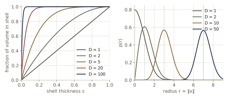
First, volume concentrates near the surface. The volume of a ball of radius \(r\) in \(D\) dimensions scales as \(r^D\), say \(V_D(r) = K_D r^D\) with \(K_D\) depending only on \(D\). The fraction of the unit ball’s volume lying in the outer shell between radius \(1 - \epsilon\) and 1 is therefore
\[\frac{V_D(1) - V_D(1 - \epsilon)}{V_D(1)} = 1 - (1 - \epsilon)^D ,\]which tends to 1 as \(D\) grows, however thin the shell.
Second, a Gaussian is not where its density is highest. For a standard Gaussian in \(D\) dimensions, the probability of lying at distance between \(r\) and \(r + \delta r\) from the origin is the density times the volume of that thin shell, \(S_D r^{D-1} \delta r\), where \(S_D = 2\pi^{D/2} / \Gamma(D/2)\) is the surface area of the unit sphere. So the density of the radius is
\[p(r) = \frac{S_D\, r^{D-1}}{(2\pi)^{D/2}} \exp\left( -\frac{r^2}{2} \right).\]The factor \(r^{D-1}\) grows and the exponential decays; setting the derivative of \((D - 1)\ln r - r^2/2\) to zero puts the peak at \(\hat r = \sqrt{D - 1} \approx \sqrt{D}\). The density \(p(\mathbf{x})\) itself is highest at the origin, yet almost no probability mass is near it: the ratio of the density at the origin to the density at radius \(\hat r\) is \(\exp(\hat r^2 / 2) = \exp((D-1)/2)\). We check all of this numerically, with the radial density written in log form to avoid overflow.
def log_radial_density(r, D):
    """ln p(r) for the radius of a standard Gaussian in D dimensions."""
    return (np.log(2) - gammaln(D / 2) - (D / 2) * np.log(2) + (D - 1) * np.log(r) - r ** 2 / 2)

r = np.linspace(1e-6, 40, 200_001)
print("  D   shell(eps=0.05)   int p(r) dr   argmax p   sqrt(D-1)   sample mean ||x||   sd")
for D in [1, 2, 10, 100, 784]:
    p = np.exp(log_radial_density(r, D))
    norms = np.linalg.norm(rng.standard_normal((20_000, D)), axis=1)
    print(f"{D:3d}   {1 - 0.95 ** D:14.4f}   {np.trapezoid(p, r):11.4f}   {r[p.argmax()]:8.3f}"
          f"   {np.sqrt(D - 1):9.3f}   {norms.mean():17.3f}   {norms.std():.3f}")
log10_ratio = (784 - 1) / 2 / np.log(10)                     # exp((D-1)/2) as a power of 10
print(f"D = 784: density at origin / density at the typical radius = 10^{log10_ratio:.0f}")
  D   shell(eps=0.05)   int p(r) dr   argmax p   sqrt(D-1)   sample mean ||x||   sd
  1           0.0500        1.0000      0.000       0.000               0.796   0.599
  2           0.0975        1.0000      1.000       1.000               1.253   0.656
 10           0.4013        1.0000      3.000       3.000               3.081   0.698
100           0.9941        1.0000      9.950       9.950               9.977   0.707
784           1.0000        1.0000     27.982      27.982              27.988   0.707
D = 784: density at origin / density at the typical radius = 10^170
With \(D = 784\), the number of pixels in an MNIST digit, 5% of the radius holds essentially all of the volume. The Gaussian samples sit at distance \(\sqrt{D}\) from the origin with a spread of about 0.7 whatever the dimension (once it is more than a few), so in high dimensions they occupy a thin shell. And the density at the center is \(10^{170}\) times larger than on the shell where the samples are.
A related effect is that distances concentrate. For random points in high dimensions, the nearest and the farthest neighbours of a query are at almost the same distance, which is bad news for any method built on “nearby points are similar”.
for D in [2, 10, 100, 1000]:
    X = rng.standard_normal((500, D))
    d = np.linalg.norm(X - rng.standard_normal(D), axis=1)
    print(f"D = {D:4d}   nearest / farthest distance = {d.min() / d.max():.3f}")
D =    2   nearest / farthest distance = 0.020
D =   10   nearest / farthest distance = 0.237
D =  100   nearest / farthest distance = 0.692
D = 1000   nearest / farthest distance = 0.893
Dimension is not all bad. Adding a variable can separate classes that overlap when only some of the variables are measured: two classes whose values of \(x_1\) overlap may be perfectly separable by a line in the \((x_1, x_2)\) plane. More measurements give a classifier more to work with, provided it can cope with the space they live in.
Watch out. The pictures in this course are drawn in one or two dimensions because that is what fits on a page. Use them for intuition about mechanisms, but do not trust them for statements about volume, distance, or where probability mass lies once \(D\) is large.
Data manifolds
If the curse of dimensionality were the whole story, learning from images with hundreds of thousands of pixels would be hopeless. It is not, because real data do not fill the space. They lie close to a manifold, a smooth surface of much lower dimension than the space around it.
Take one handwritten digit and rotate it. Each rotated copy is a point in \(\mathbb{R}^{784}\), and as the angle varies the points trace out a curve: a one-dimensional manifold. Shifting the digit adds two more dimensions. The manifold is curved, because pixel intensities depend on the angle in a very nonlinear way. We load a subset of MNIST and measure this.
train = datasets.MNIST(root="data", train=True, download=True)
X_img = train.data[:6000].float().div(255.).numpy()           # (6000, 28, 28), values in [0, 1]
t_img = train.targets[:6000].numpy()
X_mnist = X_img.reshape(len(X_img), -1)                        # data matrix, (N, D) = (6000, 784)

angles = np.arange(-45, 45.01, 0.5)                            # 181 angles, in degrees
curve = np.array([ndimage.rotate(X_img[0], a, reshape=False, order=1) for a in angles])
curve = curve.reshape(len(angles), -1)
step = np.linalg.norm(np.diff(curve, axis=0), axis=1).mean()
mid = curve[len(angles) // 2]                                  # the unrotated digit
other = np.linalg.norm(X_mnist[1:] - mid, axis=1).min()
print(f"digit label {t_img[0]}; neighbouring rotations (0.5 degrees apart) are {step:.2f} apart")
print(f"nearest other training image is {other:.2f} away; the two ends of the curve are "
      f"{np.linalg.norm(curve[0] - curve[-1]):.2f} apart")

def n_components(Z, level):
    """How many principal components are needed to keep `level` of the variance."""
    s = np.linalg.svd(Z - Z.mean(0), compute_uv=False)
    return int(np.searchsorted(np.cumsum(s ** 2) / np.sum(s ** 2), level) + 1)

print(f"rotation curve: {n_components(curve, 0.90)} components for 90% of variance, "
      f"{n_components(curve, 0.99)} for 99%")
digit label 5; neighbouring rotations (0.5 degrees apart) are 0.34 apart
nearest other training image is 6.55 away; the two ends of the curve are 12.21 apart
rotation curve: 5 components for 90% of variance, 11 for 99%
A one-parameter family of images needs several linear directions to describe, because the curve bends through pixel space; a linear method such as principal component analysis sees a flat subspace of dimension 5 to 11, while the curve itself is one-dimensional. The same holds for the whole data set. Compare MNIST with two data sets that have the same dimension and the same pixel statistics but no manifold structure: pixels drawn independently from Gaussians with each pixel’s mean and standard deviation, and each image’s own pixels shuffled into random positions. We count principal components and compare each point’s nearest-neighbour distance with its average distance to the rest.
def nn_ratio(Z, m=300):
    """Median over m query points of (nearest-neighbour distance) / (mean distance)."""
    Q = Z[:m]
    d2 = (Q ** 2).sum(1)[:, None] + (Z ** 2).sum(1)[None, :] - 2 * Q @ Z.T
    d = np.sqrt(np.maximum(d2, 0))
    d[np.arange(m), np.arange(m)] = np.nan                     # skip each point's own distance
    return np.median(np.nanmin(d, 1) / np.nanmean(d, 1))

X_gauss = rng.standard_normal(X_mnist.shape) * X_mnist.std(0) + X_mnist.mean(0)
X_shuffled = rng.permuted(X_mnist, axis=1)                     # shuffle pixels within each image
for name, Z in [("MNIST", X_mnist), ("Gaussian, same pixel stats", X_gauss),
                ("pixels shuffled", X_shuffled)]:
    print(f"{name:27s} 90% variance: {n_components(Z, 0.9):3d} components   "
          f"nearest/mean distance: {nn_ratio(Z):.2f}")
MNIST                       90% variance:  84 components   nearest/mean distance: 0.46
Gaussian, same pixel stats  90% variance: 292 components   nearest/mean distance: 0.88
pixels shuffled             90% variance: 633 components   nearest/mean distance: 0.79
Real digits need about 84 of 784 directions for 90% of the variance, while shuffled pixels need hundreds. And a real digit has a neighbour at less than half the typical distance, while in the structureless data sets every point is about equally far from every other, as the concentration of distances predicts. Real images are strongly correlated from pixel to pixel; a random image, drawn pixel by pixel, looks like noise, and essentially never like a photograph. Natural images occupy a vanishingly small part of image space.
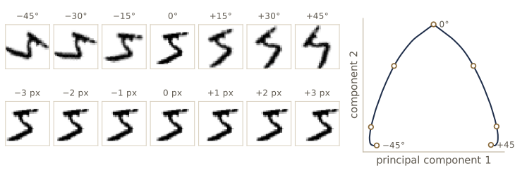
This changes the counting argument. If basis functions only need to cover the manifold, their number grows exponentially with the manifold’s dimension, not with the dimension of pixel space, and increasing the resolution of the camera adds pixels without adding dimensions to the manifold. Moreover, a task often depends on only some directions along the manifold: to read a digit we need its shape, not its position. A good model should find the manifold and the relevant directions within it. That is what learned basis functions do.
Data-dependent basis functions
For a long time the standard answer was to design features by hand, using domain knowledge and trial and error. That approach has been largely replaced by features learned from data, with domain knowledge moving into the design of network architectures (convolutions for images in module 10, for example).
A first data-dependent idea is to put one basis function on each training point, so that the basis automatically follows the data manifold. Radial basis functions do this with
\[\phi_n(\mathbf{x}) = \exp\left( -\frac{\lVert \mathbf{x} - \mathbf{x}_n \rVert^2}{s^2} \right),\]where \(s\) sets the width. With \(N\) training points this means \(N\) basis functions and an \(N \times N\) design matrix, which becomes expensive for large data sets and needs careful regularization. The support vector machine also centers basis functions on training points but keeps only a subset of them; the subset is still typically large and grows with the data, and the basic model gives neither probabilities nor a natural multiclass extension. Both are treated in Intro to ML, module 06 and module 07. Neural networks take the other route: a fixed number of basis functions, each with learnable parameters, fitted to the data by gradient-based optimization. They scale to very large data sets and, as we will see, can learn hierarchies of features.
Multilayer networks
The idea of a neural network fits in one sentence: make each basis function \(\phi_j\) a function of the same form as the model itself, a nonlinearity applied to a weighted sum of the inputs, with weights that are learned along with everything else. The only requirement is differentiability in the parameters, so that the whole model can be trained by gradient descent (module 07).
With two layers of learnable parameters, the first layer forms \(M\) linear combinations of the \(D\) inputs,
\[a^{(1)}_j = \sum_{i=1}^{D} w^{(1)}_{ji} x_i + w^{(1)}_{j0}, \qquad j = 1, \dots, M.\]The superscript names the layer. The \(w^{(1)}_{ji}\) are weights, the \(w^{(1)}_{j0}\) are biases, and the \(a^{(1)}_j\) are pre-activations. Each passes through a differentiable nonlinear activation function \(h\),
\[z^{(1)}_j = h\left(a^{(1)}_j\right),\]and the \(z^{(1)}_j\), the learned basis functions, are called hidden units. The second layer combines them the same way,
\[a^{(2)}_k = \sum_{j=1}^{M} w^{(2)}_{kj} z^{(1)}_j + w^{(2)}_{k0}, \qquad k = 1, \dots, K,\]and an output activation \(f\) gives the network outputs \(y_k = f(a^{(2)}_k)\). The choice of \(f\) follows the kind of target, exactly as for single-layer models; the section on error functions below makes it precise.
Parameter matrices
As in module 04, the biases can be absorbed by adding a constant input \(x_0 = 1\) (and a constant hidden unit \(z_0 = 1\)), so that \(a^{(1)}_j = \sum_{i=0}^{D} w^{(1)}_{ji} x_i\). Collecting the weights into matrices, the whole network is
\[\mathbf{y}(\mathbf{x}, \mathbf{w}) = f\left( \mathbf{W}^{(2)} h\left( \mathbf{W}^{(1)} \mathbf{x} \right) \right),\]with \(h\) and \(f\) applied element by element. For a data matrix \(\mathbf{X}\) with one row per example (\(N \times D\)), the pre-activations of all hidden units for all examples are one matrix product, \(\mathbf{A}^{(1)} = \mathbf{X} \mathbf{W}^{(1)\mathrm{T}} + \mathbf{1}\mathbf{b}^{(1)\mathrm{T}}\), where \(\mathbf{W}^{(1)}\) is \(M \times D\) and \(\mathbf{b}^{(1)}\) holds the biases. In code the bias is added by broadcasting. We write a network with any number of layers as a list of (weight matrix, bias vector) pairs.
def init_mlp(sizes, rng):
    """Parameters for layer sizes [D, M1, ..., K]: W is (out, in) with entries N(0, 1/in)."""
    return [(rng.normal(0, 1 / np.sqrt(m_in), (m_out, m_in)), np.zeros(m_out))
            for m_in, m_out in zip(sizes[:-1], sizes[1:])]

def forward_np(params, X, h=np.tanh):
    """Forward pass for all rows of X: hidden layers use h, the output layer is linear."""
    Z = X
    for l, (W, b) in enumerate(params):
        A = Z @ W.T + b                                  # a_j = sum_i w_ji z_i + w_j0
        Z = A if l == len(params) - 1 else h(A)          # z_j = h(a_j)
    return Z

def n_params(sizes):
    return sum(m_out * (m_in + 1) for m_in, m_out in zip(sizes[:-1], sizes[1:]))

params = init_mlp([3, 4, 2], rng)
X = rng.normal(size=(5, 3))
Y = forward_np(params, X)

(W1, b1), (W2, b2) = params                              # row 0 again, as explicit sums
x = X[0]
z = [np.tanh(sum(W1[j, i] * x[i] for i in range(3)) + b1[j]) for j in range(4)]
y = [sum(W2[k, j] * z[j] for j in range(4)) + b2[k] for k in range(2)]
W1_tilde = np.hstack([b1[:, None], W1])                  # absorb the bias: x_0 = 1
z_tilde = np.tanh(W1_tilde @ np.concatenate([[1.0], x]))
print("matrix form :", Y[0])
print("explicit sum:", np.array(y), "  bias absorbed, hidden layer matches:",
      np.allclose(z_tilde, z))
print(f"parameters in a 784-128-10 network: {n_params([784, 128, 10]):,d}")
matrix form : [-0.3352 -0.128 ]
explicit sum: [-0.3352 -0.128 ]   bias absorbed, hidden layer matches: True
parameters in a 784-128-10 network: 101,770
The matrix form is the one to keep in mind: a layer is a matrix product, a bias added by broadcasting, and an element-wise nonlinearity. A network of 101,770 parameters, a small one by today’s standards, is three lines of NumPy.
From here on we also use PyTorch, which provides the same arrays (called tensors) plus two things we need for training: automatic differentiation, which computes the gradient of any scalar built from tensor operations, and ready-made optimizers. Module 08 derives how automatic differentiation works and rebuilds it from scratch; until then we use it as a trusted tool. If PyTorch is new to you, the EAS 510 notes on tensors are a gentle start. First we check that nn.Linear computes the same thing as our NumPy code.
net = nn.Sequential(nn.Linear(3, 4), nn.Tanh(), nn.Linear(4, 2)).double()
with torch.no_grad():                                     # copy our NumPy parameters
    for layer, (W, b) in zip([net[0], net[2]], params):
        layer.weight.copy_(torch.from_numpy(W))           # nn.Linear stores W with shape (out, in)
        layer.bias.copy_(torch.from_numpy(b))
Y_torch = net(torch.from_numpy(X))
print("PyTorch matches NumPy:", torch.allclose(Y_torch, torch.from_numpy(Y)))
print("parameter count:", sum(p.numel() for p in net.parameters()), "=", n_params([3, 4, 2]))
PyTorch matches NumPy: True
parameter count: 26 = 26
Universal approximation
How much can a two-layer network represent? A series of results from the late 1980s shows that, for a wide range of activation functions, a two-layer network with a linear output can approximate any continuous function on a compact subset of \(\mathbb{R}^D\) to any accuracy, given enough hidden units. Networks are therefore called universal approximators.
We test this on three functions on \([-1, 1]\) with increasing difficulty for a smooth approximator: a smooth oscillation \(\sin(2.5\pi x)\), a kink \(\lvert x \rvert - 0.5\), and a step at \(x = 0.2\). For each we train two-layer tanh networks of width \(M = 1, 2, 4, \dots, 32\) by minimizing the mean squared error with the Adam optimizer (module 07 explains Adam). Eighteen separate training runs of this size spend most of their time on per-call overhead, so we train them all at once: every parameter gets a leading axis that indexes the network, hidden units beyond a network’s width are multiplied by zero, and the loss is the sum of the eighteen losses. Because the networks share no parameters, the gradient of the sum with respect to one network’s parameters is that network’s own gradient, and Adam’s update of each parameter depends only on that parameter’s gradient; the result is identical to eighteen separate runs.
x_grid = np.linspace(-1, 1, 200)
targets = {"smooth": lambda x: np.sin(2.5 * np.pi * x),
           "kink":   lambda x: np.abs(x) - 0.5,
           "step":   lambda x: (x > 0.2).astype(float)}
widths = [1, 2, 4, 8, 16, 32]

def fit_stack(T, widths, steps=2500, lr=0.01, seed=0):
    """Train one two-layer tanh network per column of T (N, G), with widths[g] hidden units."""
    torch.manual_seed(seed)
    G, M_max = len(widths), max(widths)
    M = torch.tensor(widths, dtype=torch.float32)[:, None]
    mask = (torch.arange(M_max) < M).float()                     # (G, M_max): 1 = unit exists
    W1 = (3 * (2 * torch.rand(G, M_max) - 1)).requires_grad_()   # input weights, U(-3, 3)
    b1 = (3 * (2 * torch.rand(G, M_max) - 1)).requires_grad_()
    W2 = ((2 * torch.rand(G, M_max) - 1) / M.sqrt()).requires_grad_()
    b2 = torch.zeros(G, requires_grad=True)
    X = torch.tensor(x_grid, dtype=torch.float32)[:, None, None]  # (N, 1, 1)
    T = torch.tensor(T, dtype=torch.float32)
    net = lambda: (torch.tanh(X * W1 + b1) * mask * W2).sum(-1) + b2   # (N, G)
    opt = torch.optim.Adam([W1, b1, W2, b2], lr=lr)
    for step in range(steps):
        loss = ((net() - T) ** 2).mean(0).sum()                 # sum over networks of their MSE
        opt.zero_grad(); loss.backward(); opt.step()            # gradients by autograd
    with torch.no_grad():
        Y = net()
    return Y.numpy(), ((Y - T) ** 2).mean(0).sqrt().numpy()

T_all = np.stack([f(x_grid) for f in targets.values() for M in widths], axis=1)
Y_fits, rms = fit_stack(T_all, widths * len(targets))
print("RMS error    " + "".join(f"M = {M:<5d}" for M in widths))
for name, row in zip(targets, rms.reshape(len(targets), -1)):
    print(f"{name:10s}" + "".join(f"{e:9.4f}" for e in row))
RMS error    M = 1    M = 2    M = 4    M = 8    M = 16   M = 32
smooth       0.7079   0.5863   0.0711   0.0203   0.0162   0.0098
kink         0.2901   0.0265   0.0117   0.0079   0.0082   0.0059
step         0.1049   0.0992   0.0956   0.0787   0.0703   0.0576
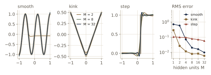
The oscillation has five half-periods on the interval and needs roughly one tanh unit for each: one or two units capture at most a single bump, four get the shape (RMS error 0.07), eight reach 0.02, and 32 about 0.01. The kink is already captured by two units, which can combine into something close to \(\lvert x \rvert\), and improves further with width. The step is the hard case. A tanh unit can make a sharp step only with a very large input weight, and gradient descent grows weights slowly, so the fits stay smooth across the jump and the error decreases slowly. Sometimes the error even rises slightly with width; that is the optimizer, not the representation, since a wider network can always represent what a narrower one can.
This is the first of several caveats. The theorems say a good network exists. They do not say how many units it needs (for some functions the number grows exponentially with \(D\)), nor that training will find it. And the no-free-lunch theorem (module 09) says no learning method is best for every problem. Finally, even when two layers suffice in principle, networks with many layers can do the same job with far fewer parameters, as we will see shortly.
Hidden-unit activation functions
The output activation is dictated by the kind of target. For the hidden units the only hard requirement is differentiability (almost everywhere), which leaves a lot of room. Usually all hidden units share one activation function.
The simplest choice, the identity, does not work: a composition of linear maps is linear, so a network of linear units is no more expressive than one linear layer. There is one twist. If a hidden layer has fewer units \(M\) than both the inputs \(D\) and the outputs \(K\), the network computes a linear map of rank at most \(M\) with \(M(D + K)\) parameters instead of \(DK\). Such a linear bottleneck is closely related to principal component analysis (module 16).
D_in, M_hid, K_out = 6, 2, 5
W_lin1, W_lin2 = rng.normal(size=(M_hid, D_in)), rng.normal(size=(K_out, M_hid))
W_eff = W_lin2 @ W_lin1                                  # the whole linear network
print(f"effective matrix {W_eff.shape}, rank {np.linalg.matrix_rank(W_eff)}; "
      f"{M_hid * (D_in + K_out)} parameters vs {D_in * K_out} for a full linear map")
effective matrix (5, 6), rank 2; 22 parameters vs 30 for a full linear map
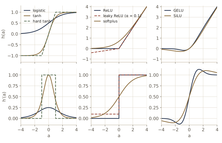
Nonlinear activation functions come in two families. The sigmoidal ones saturate at both ends:
- the logistic sigmoid \(\sigma(a) = 1/(1 + e^{-a})\), historically the first choice;
- \(\tanh(a) = (e^a - e^{-a})/(e^a + e^{-a})\), which is a rescaled logistic, \(\tanh(a) = 2\sigma(2a) - 1\), so a network with one can be turned into an equivalent network with the other by adjusting the weights and biases (exercise 3); in training they still behave differently, because the initialization has to be adapted;
- hard tanh, \(\max(-1, \min(1, a))\), a piecewise-linear version.
Their derivatives decay exponentially for large \(\lvert a \rvert\). A unit whose pre-activation is large in magnitude passes back almost no gradient; this is the source of vanishing gradients in deep sigmoidal networks, taken up in module 07. Since \(\sigma'(a) = \sigma(a)(1 - \sigma(a)) \le 1/4\), a signal passing back through \(L\) logistic units shrinks by at least \(4^{-L}\) from the activation derivatives alone.
The rectifier family keeps a nonzero slope for large positive inputs:
- the rectified linear unit or ReLU, \(\max(0, a)\), the default in most practice: cheap, well suited to low-precision arithmetic, and much less sensitive to initialization than sigmoidal units. Its derivative is undefined at \(a = 0\); implementations pick 0 there and nothing goes wrong in practice;
- the leaky ReLU, \(\max(0, a) + \alpha \min(0, a)\) with \(0 < \alpha < 1\), which keeps a small gradient for negative inputs so that a unit that is switched off for every example can still recover; with \(\alpha = -1\) it becomes \(\lvert a \rvert\), and with a learned \(\alpha\) per unit it is called a parametric ReLU;
- softplus, \(\zeta(a) = \ln(1 + e^a)\), a smooth ReLU whose derivative is exactly \(\sigma(a)\);
- smooth, slightly non-monotonic variants used in many modern architectures: GELU, \(a\,\Phi(a)\) with \(\Phi\) the standard normal distribution function, and SiLU (also called swish), \(a\,\sigma(\beta a)\), usually with \(\beta = 1\).
We implement each function and its derivative in NumPy and check the derivatives against PyTorch’s autograd applied to PyTorch’s own versions of the functions.
Phi = lambda a: 0.5 * (1 + erf(a / np.sqrt(2)))           # standard normal CDF
phi = lambda a: np.exp(-a ** 2 / 2) / np.sqrt(2 * np.pi)   # standard normal density
alpha = 0.1
activations = {   # name: (h, h', the torch version)
    "logistic":  (expit, lambda a: expit(a) * (1 - expit(a)), torch.sigmoid),
    "tanh":      (np.tanh, lambda a: 1 - np.tanh(a) ** 2, torch.tanh),
    "hard tanh": (lambda a: np.clip(a, -1, 1), lambda a: (np.abs(a) < 1) * 1.0, F.hardtanh),
    "ReLU":      (lambda a: np.maximum(0, a), lambda a: (a > 0) * 1.0, F.relu),
    "leaky ReLU": (lambda a: np.maximum(0, a) + alpha * np.minimum(0, a),
                   lambda a: np.where(a > 0, 1.0, alpha), lambda a: F.leaky_relu(a, alpha)),
    "softplus":  (lambda a: np.logaddexp(0, a), expit, F.softplus),
    "GELU":      (lambda a: a * Phi(a), lambda a: Phi(a) + a * phi(a), F.gelu),
    "SiLU":      (lambda a: a * expit(a), lambda a: expit(a) * (1 + a * (1 - expit(a))), F.silu),
}
a = np.linspace(-6, 6, 1201) + 1e-3                      # a grid that avoids the kinks at 0 and +-1
print("function     max|h - torch|  max|h' - autograd|    h'(-5)    h'(0.5)   h'(5)")
for name, (h, dh, h_torch) in activations.items():
    a_t = torch.tensor(a, requires_grad=True)
    out = h_torch(a_t)
    grad, = torch.autograd.grad(out.sum(), a_t)          # d h / d a at every grid point
    print(f"{name:11s}  {np.abs(h(a) - out.detach().numpy()).max():12.1e}"
          f"  {np.abs(dh(a) - grad.numpy()).max():17.1e}"
          + "".join(f"  {dh(np.array(v)):8.4f}" for v in [-5.0, 0.5, 5.0]))
function     max|h - torch|  max|h' - autograd|    h'(-5)    h'(0.5)   h'(5)
logistic          1.1e-16            9.7e-17    0.0066    0.2350    0.0066
tanh              1.1e-16            2.8e-16    0.0002    0.7864    0.0002
hard tanh         0.0e+00            0.0e+00    0.0000    1.0000    0.0000
ReLU              0.0e+00            0.0e+00    0.0000    1.0000    1.0000
leaky ReLU        0.0e+00            0.0e+00    0.1000    1.0000    1.0000
softplus          8.9e-16            2.2e-16    0.0067    0.6225    0.9933
GELU              4.4e-16            2.2e-16   -0.0000    0.8675    1.0000
SiLU              8.9e-16            2.2e-16   -0.0265    0.7400    1.0265
The two implementations agree to rounding error. The last columns show saturation: at \(a = 5\) the logistic and tanh derivatives are already below 0.01, and at \(a = -5\) as well, while the rectifiers keep slope 1 on the positive side. The price of ReLU is the flat negative side: a ReLU unit with \(a < 0\) for every training example receives no gradient at all. Leaky ReLU, softplus, GELU, and SiLU all leak a little gradient there.
In practice. Start with ReLU (or GELU, which many transformer architectures use). Reach for tanh or the logistic sigmoid inside a network only when you need a bounded output from a unit, as in the gates of recurrent networks, and never as a default for deep stacks.
Weight-space symmetries
Different weight vectors can compute exactly the same function. For a two-layer tanh network with \(M\) hidden units, two kinds of change leave the input-output map untouched:
- sign flips: negate all weights and the bias going into hidden unit \(j\) and all weights coming out of it. Since \(\tanh(-a) = -\tanh(a)\), the unit’s output changes sign and the outgoing weights change it back. There are \(2^M\) ways to choose which units to flip;
- permutations: relabel the hidden units, moving each unit’s incoming and outgoing weights together. There are \(M!\) orderings.
So every weight vector belongs to a set of \(2^M M!\) equivalent ones, and for a network with several hidden layers the factors multiply. Apart from accidental coincidences, these are all the discrete symmetries, and similar results hold for many other activation functions. We enumerate all 48 transformations for \(M = 3\) and check that every one gives the same outputs and a different weight vector.
def two_layer(W1, b1, W2, b2, X, h=np.tanh):
    return h(X @ W1.T + b1) @ W2.T + b2

M = 3
(W1, b1), (W2, b2) = init_mlp([2, M, 1], rng)
b1 = rng.normal(size=M)                                   # nonzero biases, so flips are visible
X = rng.normal(size=(50, 2))
Y_ref = two_layer(W1, b1, W2, b2, X)
vectors, max_diff = set(), 0.0
for signs in product([1.0, -1.0], repeat=M):
    for perm in permutations(range(M)):
        P = np.eye(M)[list(perm)] * np.array(signs)[:, None]     # permute rows, then flip signs
        V1, c1, V2 = P @ W1, P @ b1, W2 @ P.T                     # P is orthogonal: P^T undoes it
        max_diff = max(max_diff, np.abs(two_layer(V1, c1, V2, b2, X) - Y_ref).max())
        vectors.add(tuple(np.round(np.concatenate([V1.ravel(), c1, V2.ravel()]), 10)))
print(f"transformations: {2 ** M * factorial(M)}   distinct weight vectors: {len(vectors)}"
      f"   largest change in output: {max_diff:.1e}")
transformations: 48 distinct weight vectors: 48 largest change in output: 1.1e-16
ReLU is not odd, so sign flips do not work for it. It has a different, continuous symmetry instead: for any \(c > 0\), \(\max(0, ca) = c \max(0, a)\), so scaling a unit’s incoming weights and bias by \(c\) and its outgoing weights by \(1/c\) changes nothing.
relu = lambda a: np.maximum(0, a)
S = np.diag([-1.0, 1.0, 1.0])                             # flip unit 1
C = np.diag([0.2, 3.0, 7.5])                              # rescale all three units
Y_relu = two_layer(W1, b1, W2, b2, X, relu)
flip = two_layer(S @ W1, S @ b1, W2 @ S, b2, X, relu)
scale = two_layer(C @ W1, C @ b1, W2 / np.diag(C), b2, X, relu)   # W2 C^-1
print(f"ReLU, sign flip:       max change {np.abs(flip - Y_relu).max():.3f}")
print(f"ReLU, positive rescale: max change {np.abs(scale - Y_relu).max():.1e}")
ReLU, sign flip:       max change 0.122
ReLU, positive rescale: max change 4.4e-16
For training these symmetries rarely matter: we want one good weight vector, and it does not matter which of the equivalent copies we land on. They matter when we reason about the error surface (every minimum comes with many copies) and in Bayesian treatments that integrate over weight space, where each mode is counted \(2^M M!\) times (Intro to ML, module 05 works this through).
Deep networks
Nothing stops us from repeating the construction. A network with \(L\) layers of learnable parameters computes, for \(l = 1, \dots, L\),
\[\mathbf{z}^{(l)} = h^{(l)}\left( \mathbf{W}^{(l)} \mathbf{z}^{(l-1)} \right),\]with \(\mathbf{z}^{(0)} = \mathbf{x}\) the input, \(\mathbf{z}^{(L)} = \mathbf{y}\) the output, \(h^{(l)}\) the activation function of layer \(l\) (the output activation for \(l = L\)), and \(\mathbf{W}^{(l)}\) holding the weights and biases of layer \(l\). A network with more than two layers is called a deep neural network. For many years two-layer networks dominated because deeper ones were hard to train; the techniques of modules 07 and 09 changed that.
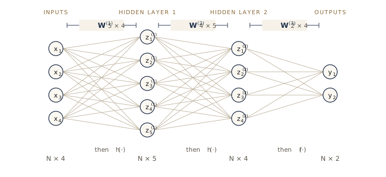
Counting layers is a source of confusion. The two-layer network above is also called a three-layer network (counting the input as a layer of units) or a single-hidden-layer network. We count layers of learnable weights, since that is what determines what a network can do. Our forward_np already handles any depth, since params can be a list of any length.
Depth and the number of linear pieces
Why go deep if two layers are already universal? One reason is efficiency. A network of ReLU units computes a continuous piecewise-linear function, and the number of linear pieces it can make grows much faster with depth than with width. Theoretical results make this precise (Montúfar and coauthors, 2014, count the linear regions and show they can grow exponentially in depth but only polynomially in width); here we build an example by hand.
For one input, a two-layer ReLU network with \(M\) hidden units is a sum of \(M\) functions, each with a single kink, so it has at most \(M + 1\) linear pieces. Now consider the tent map on \([0, 1]\),
\[g(x) = 2\max(0, x) - 4\max\left(0, x - \tfrac12\right) = \begin{cases} 2x & x \le \tfrac12, \\ 2 - 2x & x > \tfrac12, \end{cases}\]which is one layer of two ReLU units followed by a linear combination. It maps \([0, 1]\) onto itself, going up and then down. Composing it with itself, \(g(g(x))\) goes up and down twice, and each further composition doubles the number of teeth: \(g^{(L)} = g \circ \cdots \circ g\) has \(2^{L-1}\) teeth and \(2^L\) linear pieces. As a network, \(g^{(L)}\) has \(L\) hidden layers of 2 ReLU units each, \(2L\) units in total, while a two-layer network needs at least \(2^L - 1\) units to produce \(2^L\) pieces. We build the deep network as weight matrices and count its pieces by evaluating on a fine grid of dyadic points, where the kinks fall exactly on grid points.
def sawtooth_params(L):
    """Weights of the network computing g composed L times: L hidden layers of 2 ReLU units."""
    b = np.array([0.0, -0.5])
    params = [(np.array([[1.0], [1.0]]), b)]                    # a = (x, x - 1/2)
    for l in range(L - 1):                   # next a = (g, g - 1/2), with g = 2 z1 - 4 z2
        params.append((np.array([[2.0, -4.0], [2.0, -4.0]]), b))
    params.append((np.array([[2.0, -4.0]]), np.zeros(1)))       # output g = 2 z1 - 4 z2
    return params

def count_pieces(y, x):
    slopes = np.round(np.diff(y) / np.diff(x), 6)
    return 1 + int(np.sum(slopes[1:] != slopes[:-1]))

x_dy = np.linspace(0, 1, 2 ** 12 + 1)[:, None]                   # dyadic grid, spacing 2^-12
print(" L   hidden units   linear pieces   two-layer network needs")
for L in range(1, 7):
    y_saw = forward_np(sawtooth_params(L), x_dy, h=relu)[:, 0]
    assert np.allclose(y_saw[::2 ** (12 - L)], np.arange(2 ** L + 1) % 2)   # teeth hit 0 and 1
    pieces = count_pieces(y_saw, x_dy[:, 0])
    print(f"{L:2d}   {2 * L:12d}   {pieces:13d}   {2 ** L - 1:10d} units")
 L   hidden units   linear pieces   two-layer network needs
 1              2               2            1 units
 2              4               4            3 units
 3              6               8            7 units
 4              8              16           15 units
 5             10              32           31 units
 6             12              64           63 units
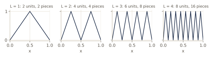
Six layers with 12 units in total produce 64 linear pieces; a single hidden layer would need 63 units. The general lesson is that composition multiplies while addition only adds. Whether a trained network actually uses its depth this way is a separate question, and functions this regular are rare in practice; but the construction shows that depth can buy expressiveness that width pays for exponentially.
Hierarchical representations
A stronger reason for depth is the kind of structure it builds in. A deep network computes its output through a sequence of intermediate representations, each a function of the one before. That is an inductive bias, a preference built into the model before it sees data: the bias toward functions that are compositions of simpler functions. Much of the world is like that. In an image, edges combine into textures and simple shapes, shapes into parts, and parts into objects; a network for recognizing birds can detect edges in its first layers, combine them into feathers and beaks, and combine those into a bird. The same view runs in reverse for generating images: pick objects, then their parts, then the shapes and edges that render them. At each level there are many ways to combine the pieces from the level below, so the number of things the model can express grows exponentially with the number of levels. Convolutional networks (module 10) make this hierarchy explicit for images.
Distributed representations
A second kind of compositionality lives within a single layer. If each hidden unit signals the presence of one feature, \(M\) units can represent \(M\) features. But the network can also let combinations of units carry meaning, so that \(M\) binary-ish units can in principle distinguish \(2^M\) situations. Suppose a photo of a room can have the lamp on or off, the window open or closed, and a person present or not. One unit per combination needs eight units. Three units, one per attribute, describe the same eight situations, and a classifier downstream can generalize to a combination it rarely saw (lamp on, window open, person present) because each attribute was learned from all the photos that had it. This is a distributed representation: each concept is encoded by a pattern over many units, and each unit takes part in many concepts. In real networks the attributes are not perfectly independent or perfectly aligned with single units, but the exponential capacity is the point.
Representation learning
We can read a deep network as a sequence of transformations of the data, each making the task a little easier. Look at the last hidden layer of a network trained for classification: the output layer is a linear classifier on top of it, so if the network works, the classes must be close to linearly separable there. The network has learned a nonlinear map into a space where a linear model suffices. Discovering such a map is called representation learning, and the space of hidden-layer outputs is called an embedding space. Any input, from the training set or not, can be mapped into it by a forward pass.
Representations become especially valuable when labels are scarce and unlabelled data are plentiful. Learning from unlabelled data is unsupervised learning (or, when the training signal is manufactured from the data itself, self-supervised learning). One classic method trains a network to reproduce its input through a narrow hidden layer, which forces it to compress; such networks are autoencoders (module 19). Historically, unsupervised pre-training of each layer in turn was how the first deep fully connected networks were trained successfully, until it turned out that with the right initialization, activation functions, and data, purely supervised training from scratch works. Pre-training on unlabelled data remains central elsewhere, most visibly in language models, where transformers (module 12) are first trained on large amounts of raw text.
Transfer learning
A representation learned for one task can help with another. In transfer learning we train a network on a task B with plentiful data, then reuse part of it for a related task A with little data. The two tasks need the same kind of input and some shared structure, so that the features useful for B are useful for A. For images, early layers tend to learn generic features and later layers task-specific ones, which is why transfer works so well for image models.
There are three standard ways to reuse the network. We can keep the early layers frozen as a fixed feature extractor and train only a new output layer; this is cheap, because the new data need to go through the frozen layers only once, after which we train a small model on the resulting features. With more data we can retrain several of the final layers. Or we can fine-tune the whole network on task A, starting from the pre-trained weights, with a small learning rate and few iterations so that it does not overfit the small data set. Learning the parameters on task B is called pre-training.
We try this on a pair of related tasks built from MNIST. Our digits are placed at random positions on a \(34 \times 34\) canvas (shifted by up to 3 pixels in each direction), as a camera that is not perfectly aimed would record them. Task B is to classify digits 0 to 4, with about 10,000 labelled images. Task A is to classify digits 5 to 9, with only a handful of labels per class. First the data. We place the images with index arithmetic on the whole batch at once, which the tensor section below explains.
S = 3                                                   # maximum shift in pixels
C = 28 + 2 * S                                          # canvas size, 34

def place(imgs, dy, dx):
    """Put each 28x28 image on a CxC canvas with its top-left corner at (dy, dx) in [0, 2S]."""
    P = F.pad(imgs, (2 * S, 2 * S, 2 * S, 2 * S))       # (N, 40, 40): room for every shift
    rows = dy[:, None] + torch.arange(C)                # (N, C) row indices of each crop
    cols = dx[:, None] + torch.arange(C)
    n = torch.arange(len(imgs))[:, None, None]
    return P[n, rows[:, :, None], cols[:, None, :]].reshape(len(imgs), -1)   # (N, C*C)

def random_place(imgs, gen):
    offsets = torch.randint(0, 2 * S + 1, (2, len(imgs)), generator=gen)
    return place(imgs, offsets[0], offsets[1])

test = datasets.MNIST(root="data", train=False, download=True)
I_tr, y_tr = train.data[:20000].float().div(255.), train.targets[:20000]
I_te, y_te = test.data[:4000].float().div(255.), test.targets[:4000]
gen = torch.Generator().manual_seed(6)
X_tr, X_te = random_place(I_tr, gen), random_place(I_te, gen)
in_B, in_B_te = y_tr < 5, y_te < 5                     # task B: digits 0-4 (plenty of labels)
XB, tB, XB_te, tB_te = X_tr[in_B], y_tr[in_B], X_te[in_B_te], y_te[in_B_te]
XA, tA = X_tr[~in_B], y_tr[~in_B] - 5                  # task A: digits 5-9, relabelled 0-4
XA_te, tA_te = X_te[~in_B_te], y_te[~in_B_te] - 5
print("task B train", tuple(XB.shape), "  task A pool", tuple(XA.shape),
      "  task A test", tuple(XA_te.shape))
task B train (10225, 1156) task A pool (9775, 1156) task A test (1936, 1156)
Now we pre-train a two-layer ReLU network with 256 hidden units on task B, with the cross-entropy error (derived below) and mini-batches of 128 examples for 5 passes over the data. The gradients come from autograd.
def accuracy(net, X, t):
    with torch.no_grad():
        return (net(X).argmax(1) == t).float().mean().item()

def train_minibatch(net, X, t, epochs, lr, batch=128, seed=0):
    g = torch.Generator().manual_seed(seed)
    opt = torch.optim.Adam(net.parameters(), lr=lr)
    for epoch in range(epochs):
        perm = torch.randperm(len(X), generator=g)
        for i in range(0, len(X), batch):
            idx = perm[i:i + batch]
            loss = F.cross_entropy(net(X[idx]), t[idx])
            opt.zero_grad(); loss.backward(); opt.step()
    return net

def train_fullbatch(net, X, t, steps, lr, weight_decay=0.0):
    opt = torch.optim.Adam(net.parameters(), lr=lr, weight_decay=weight_decay)
    for step in range(steps):
        loss = F.cross_entropy(net(X), t)
        opt.zero_grad(); loss.backward(); opt.step()
    return net

torch.manual_seed(6)
net_B = nn.Sequential(nn.Linear(C * C, 256), nn.ReLU(), nn.Linear(256, 5))
train_minibatch(net_B, XB, tB, epochs=5, lr=1e-3)
body = net_B[:2]                                       # the hidden layer: pixels -> 256 features
print(f"task B test accuracy: {accuracy(net_B, XB_te, tB_te):.3f}")
task B test accuracy: 0.955
For task A we draw \(n\) labelled examples per class, for \(n = 5, 20, 50\) and three random draws each, and compare four methods on the task A test images:
- pixels: a linear softmax classifier on the raw pixels;
- scratch: the same two-layer network as for task B, trained from random weights on the few labels;
- frozen: the task B hidden layer as a fixed feature extractor, with a new linear softmax layer on top;
- fine-tuned: the frozen model, then all its weights trained further with a small learning rate.
The linear classifiers (the Probe below) standardize each input feature using the unlabelled task A images and use a little weight decay. Note that the features of all task A images are computed once, with one forward pass.
class Probe(nn.Module):
    """Linear softmax classifier on standardized features (statistics from unlabelled data)."""
    def __init__(self, H_unlabelled, K=5):
        super().__init__()
        self.register_buffer("mu", H_unlabelled.mean(0))
        self.register_buffer("sd", H_unlabelled.std(0) + 1e-3)
        self.linear = nn.Linear(H_unlabelled.shape[1], K)
    def forward(self, H):
        return self.linear((H - self.mu) / self.sd)

def fit_probe(H, idx, t, seed):
    torch.manual_seed(seed)
    return train_fullbatch(Probe(H), H[idx], t, steps=200, lr=1e-2, weight_decay=1e-3)

def few_labels(t, n, seed):
    """Indices of n random examples of each of the 5 classes."""
    g = np.random.default_rng(seed)
    return torch.as_tensor(np.concatenate(
        [g.choice(np.flatnonzero(t.numpy() == k), n, replace=False) for k in range(5)]))

with torch.no_grad():
    HA, HA_te = body(XA), body(XA_te)                  # one pass through the frozen layer
results = {}
for n in [5, 20, 50]:
    for seed in range(3):
        idx = few_labels(tA, n, seed)
        t = tA[idx]
        pixels = fit_probe(XA, idx, t, seed)
        torch.manual_seed(seed)
        scratch = train_fullbatch(nn.Sequential(nn.Linear(C * C, 256), nn.ReLU(),
                                                nn.Linear(256, 5)), XA[idx], t, 120, 2e-3)
        frozen = fit_probe(HA, idx, t, seed)
        tuned = train_fullbatch(nn.Sequential(copy.deepcopy(body), copy.deepcopy(frozen)),
                                XA[idx], t, 50, 2e-4)
        results.setdefault(n, []).append([accuracy(pixels, XA_te, tA_te),
                                          accuracy(scratch, XA_te, tA_te),
                                          accuracy(frozen, HA_te, tA_te),
                                          accuracy(tuned, XA_te, tA_te)])
print("labels per class   pixels   scratch   frozen   fine-tuned   (mean test accuracy)")
for n, r in results.items():
    print(f"{n:16d}" + "".join(f"{v:9.3f}" for v in np.mean(r, axis=0)))
labels per class   pixels   scratch   frozen   fine-tuned   (mean test accuracy)
               5    0.395    0.398    0.476    0.480
              20    0.493    0.488    0.615    0.628
              50    0.579    0.596    0.752    0.772
With few labels, the features learned on digits 0 to 4 are clearly better for digits 5 to 9 than raw pixels or a network trained from scratch, and fine-tuning adds a little on top. The task B network has learned something that transfers: how to respond to strokes wherever they fall on the canvas, a skill raw pixels do not have. When we ran the same comparison on the original centered digits, the frozen features were no better than raw pixels, because for centered digits a linear classifier on pixels is already a strong template matcher and the 0 to 4 features have little to add. Transfer helps when the source task has taught the network something the target task needs and cannot learn from its own few examples.
Note. A GPU and the full data sets would change the numbers but not the ranking. With all 60,000 training images, a wider network, and a convolutional architecture (module 10), each method improves; transfer matters most in exactly the regime we simulated, where the target task has few labels.
Two relatives of transfer learning deserve a mention. In multitask learning one network learns several related tasks at once, typically with shared early layers and separate task-specific later layers, so that each task benefits from the others’ data; handwriting recognition for many writers, each with only a few samples of their own, is a natural fit, with shared layers learning strokes and a small writer-specific layer adapting to each hand. Meta-learning, or learning to learn, goes further: it trains on many tasks with the aim of adapting quickly to new tasks never seen in training, for example recognizing a new class from very few labelled examples (few-shot learning), or from a single one (one-shot learning).
Contrastive learning
Transfer learning needed labels for the source task. Contrastive learning learns a representation without them. The idea is to choose pairs of inputs that should be close in the embedding space, called positive pairs, and pairs that should be far apart, called negative pairs, and to train the network to arrange them that way. Unlike most error functions, the loss for an input is defined only relative to other inputs; there is no per-example target.
Let \(f_{\mathbf{w}}(\mathbf{x})\) be the network’s embedding of \(\mathbf{x}\), normalized to unit length. For an anchor \(\mathbf{x}\), a positive partner \(\mathbf{x}^+\), and negatives \(\mathbf{x}^-_1, \dots, \mathbf{x}^-_N\), the most widely used loss is InfoNCE (NCE stands for noise contrastive estimation):
\[E(\mathbf{w}) = -\ln \frac{\exp\left\{ f_{\mathbf{w}}(\mathbf{x})^{\mathrm{T}} f_{\mathbf{w}}(\mathbf{x}^+) \right\}}{\exp\left\{ f_{\mathbf{w}}(\mathbf{x})^{\mathrm{T}} f_{\mathbf{w}}(\mathbf{x}^+) \right\} + \sum_{n=1}^{N} \exp\left\{ f_{\mathbf{w}}(\mathbf{x})^{\mathrm{T}} f_{\mathbf{w}}(\mathbf{x}^-_n) \right\}} .\]Each inner product of unit vectors is a cosine similarity. Read the fraction as a softmax over \(N + 1\) candidates: the loss is exactly the multiclass cross-entropy for “which candidate is the positive?”, with the similarities as logits. The negatives are essential. Without them the loss would be minimized by mapping every input to the same point, a collapse that the denominator punishes. In practice the similarities are usually divided by a temperature \(\tau\) before the exponential; the formula above is \(\tau = 1\). We implement the loss in NumPy and check it against PyTorch’s cross-entropy, then look at three configurations.
def unit(v):
    return v / np.linalg.norm(v, axis=-1, keepdims=True)

def info_nce(anchor, positive, negatives, tau=1.0):
    """InfoNCE loss for one anchor (d,), one positive (d,), and negatives (N, d); unit vectors."""
    logits = np.concatenate([[anchor @ positive], negatives @ anchor]) / tau
    return -(logits[0] - logsumexp(logits))

d, N_neg = 16, 31
anchor = unit(rng.normal(size=d))
negatives = unit(rng.normal(size=(N_neg, d)))
positive = unit(anchor + 0.3 * rng.normal(size=d))        # a slightly perturbed copy
logits = torch.tensor(np.concatenate([[anchor @ positive], negatives @ anchor]))[None]
print(f"InfoNCE {info_nce(anchor, positive, negatives):.4f}   via cross-entropy "
      f"{F.cross_entropy(logits, torch.tensor([0])).item():.4f}")
cases = {"positive close, negatives random": (positive, negatives),
         "positive random (nothing learned)": (unit(rng.normal(size=d)), negatives),
         "collapsed: everything identical": (anchor, np.tile(anchor, (N_neg, 1)))}
for name, (pos, neg) in cases.items():
    print(f"{name:35s}  tau = 1: {info_nce(anchor, pos, neg):.3f}"
          f"   tau = 0.1: {info_nce(anchor, pos, neg, tau=0.1):.3f}")
print(f"collapse gives ln(N + 1) = {np.log(N_neg + 1):.3f}; "
      f"best possible at tau = 1: ln(1 + N e^-2) = {np.log(1 + N_neg * np.exp(-2)):.3f}")
InfoNCE 2.9457   via cross-entropy 2.9457
positive close, negatives random     tau = 1: 2.946   tau = 0.1: 0.594
positive random (nothing learned)    tau = 1: 3.661   tau = 0.1: 7.222
collapsed: everything identical      tau = 1: 3.466   tau = 0.1: 3.466
collapse gives ln(N + 1) = 3.466; best possible at tau = 1: ln(1 + N e^-2) = 1.648
A collapsed embedding scores \(\ln(N + 1)\), the loss of guessing uniformly among the candidates. With \(\tau = 1\) the logits lie in \([-1, 1]\), so even a perfect arrangement cannot push the loss below \(\ln(1 + N e^{-2})\); a small temperature sharpens the softmax and lets the loss reward a well-separated positive much more strongly.
What makes a contrastive method is how it picks the pairs, since that is where our prior knowledge about “same” and “different” enters:
- Instance discrimination: the positive is a randomly transformed copy of the anchor (shifted, rotated, cropped, recolored: the transformations are data augmentations, module 09), and other images serve as negatives. The representation learns to ignore the transformations.
- Supervised contrastive learning: with labels, positives are other examples of the same class and negatives are examples of other classes. This avoids treating two images of the same kind as a negative pair and depends less on the choice of augmentations.
- Cross-modal pairs: in CLIP (contrastive language-image pre-training), a positive pair is an image and its caption, embedded by two separate networks \(f_{\mathbf{w}}\) for images and \(g_{\boldsymbol{\theta}}\) for text, and mismatched images and captions are negatives. The loss is the average of two InfoNCE terms, one matching the caption against other images and one matching the image against other captions. Captioned images can be collected at scale from the web, so this is often called weakly supervised.
In a mini-batch of \(B\) positive pairs, all the other pairs in the batch serve as negatives: the \(B \times B\) matrix of similarities between the two sides of the pairs gives \(B\) softmax classification problems whose correct answers lie on the diagonal. We try instance discrimination on our shifted digits: the two sides of a pair are the same digit placed at two independent random positions. The encoder is a hidden layer of 256 ReLU units, as before, followed by a linear projection to 64 dimensions where the loss is computed (a common design; the probe uses the 256 hidden features). Training uses all 20,000 training images and no labels, with \(\tau = 0.1\) and the symmetric (two-sided) loss.
def batch_info_nce(u, v, tau):
    """Mean InfoNCE over B pairs (u_b, v_b); every other v in the batch is a negative."""
    u, v = F.normalize(u, dim=1), F.normalize(v, dim=1)
    logits = u @ v.T / tau                                 # (B, B) cosine similarities / tau
    return F.cross_entropy(logits, torch.arange(len(u)))   # the positive is on the diagonal

torch.manual_seed(6)
encoder = nn.Sequential(nn.Linear(C * C, 256), nn.ReLU())
projection = nn.Linear(256, 64)
opt = torch.optim.Adam([*encoder.parameters(), *projection.parameters()], lr=1e-3)
gen = torch.Generator().manual_seed(6)
for step in range(301):
    imgs = I_tr[torch.randint(0, len(I_tr), (128,), generator=gen)]          # labels unused
    u = projection(encoder(random_place(imgs, gen)))
    v = projection(encoder(random_place(imgs, gen)))
    loss = 0.5 * (batch_info_nce(u, v, 0.1) + batch_info_nce(v, u, 0.1))
    opt.zero_grad(); loss.backward(); opt.step()
    if step % 100 == 0:
        print(f"step {step:3d}   InfoNCE {loss.item():.3f}"
              f"   (collapse would give {np.log(128):.3f})")

with torch.no_grad():
    HC, HC_te = encoder(XA), encoder(XA_te)
print("labels per class   pixels   contrastive features (no labels used in training)")
for n in [5, 20, 50]:
    acc_c = []
    for seed in range(3):
        idx = few_labels(tA, n, seed)
        acc_c.append(accuracy(fit_probe(HC, idx, tA[idx], seed), HC_te, tA_te))
    print(f"{n:16d}   {np.mean(results[n], axis=0)[0]:.3f}    {np.mean(acc_c):.3f}")
step   0   InfoNCE 4.539   (collapse would give 4.852)
step 100   InfoNCE 0.903   (collapse would give 4.852)
step 200   InfoNCE 0.671   (collapse would give 4.852)
step 300   InfoNCE 0.437   (collapse would give 4.852)
labels per class   pixels   contrastive features (no labels used in training)
               5   0.395    0.495
              20   0.493    0.660
              50   0.579    0.778
Without a single label, 300 steps of contrastive training produce features on which a linear classifier with a few labels per class clearly beats raw pixels, and does at least as well as the features pre-trained with 10,000 labels of digits 0 to 4 (on a problem this small, don’t read much into the difference between those two). The network has learned what we asked of it: images of the same digit at different positions should look alike.
General network architectures
Layers are a convenience, not a requirement. Because a network diagram and the function it computes correspond one to one, any diagram defines a network, provided it is feed-forward: a directed graph with no cycles, so that every output is a well-defined function of the inputs. Each hidden or output unit \(k\) computes
\[z_k = h\left( \sum_{j \in \mathcal{A}(k)} w_{kj} z_j + b_k \right),\]where \(\mathcal{A}(k)\) collects the units with a connection into \(k\) (its parents in the graph) and \(b_k\) is its bias. To evaluate the network, visit the units in an order in which every unit comes after all its parents, a topological order, which exists exactly when the graph has no cycles. Python’s standard library finds one for us.
def dag_forward(parents, w, b, inputs, outputs, h=np.tanh):
    """Evaluate a feed-forward network given as a graph: parents[k] lists the units feeding k."""
    z = dict(inputs)
    for k in TopologicalSorter(parents).static_order():     # parents always come first
        if k in z:
            continue
        a = b[k] + sum(w[(k, j)] * z[j] for j in parents[k])
        z[k] = a if k in outputs else h(a)                 # linear outputs, nonlinear hidden units
    return z

parents = {"u1": ["x1", "x2"], "u2": ["u1", "x2"], "u3": ["u1", "x1"],   # skips over layers
           "y1": ["u2", "u3", "x1"], "y2": ["u1", "u3"]}
w = {(k, j): rng.normal() for k, ps in parents.items() for j in ps}
b = {k: rng.normal() for k in parents}
z = dag_forward(parents, w, b, {"x1": 0.5, "x2": -1.0}, outputs={"y1", "y2"})
print("order:", list(TopologicalSorter(parents).static_order()))
print(f"y1 = {z['y1']:.4f}   y2 = {z['y2']:.4f}")
try:
    dag_forward({**parents, "u1": ["x1", "y2"]}, {**w, ("u1", "y2"): 1.0}, b,
                {"x1": 0.5, "x2": -1.0}, outputs={"y1", "y2"})
except CycleError as err:
    print("with a connection y2 -> u1:", type(err).__name__, err.args[1])
order: ['x1', 'x2', 'u1', 'u2', 'u3', 'y1', 'y2']
y1 = -1.0130   y2 = 0.8559
with a connection y2 -> u1: CycleError ['u1', 'u3', 'y2', 'u1']
The skip connections from x1 to the output and from u1 past u2 are exactly the kind of connection that residual networks use to make very deep networks trainable (module 09). Backpropagation (module 08) works on any such graph by visiting the units in the reverse topological order.
Tensors
Data sets, activations, and parameters so far have been scalars, vectors, and matrices. Many quantities need more indices. A batch of \(N\) color images, each \(H\) pixels high and \(W\) wide with 3 color channels, is naturally a four-index array with elements \(x_{nchw}\). Arrays with any number of indices are called tensors; scalars, vectors, and matrices are the cases with 0, 1, and 2 indices. PyTorch’s convention for images is (N, C, H, W), with the example index, the batch dimension, first, and we follow it throughout the course. Tensor operations map well onto massively parallel hardware such as GPUs, which is a large part of why deep learning became practical.
Three habits make tensor code correct and fast. Keep the batch dimension first, so that a layer written for one example works on a batch unchanged. Let broadcasting add biases and combine shapes. And replace Python loops over examples, or over models, with batched operations, as we did when we trained eighteen networks at once.
batch = torch.from_numpy(X_img[:64]).unsqueeze(1)          # (N, C, H, W) = (64, 1, 28, 28)
n_bytes = batch.element_size() * batch.nelement()
print("batch", tuple(batch.shape), batch.dtype, f"{n_bytes:,d} bytes")
flat = batch.flatten(start_dim=1)                           # (64, 784): one row per example
layer = nn.Linear(784, 128)
manual = flat @ layer.weight.T + layer.bias                 # (64, 128) + (128,): broadcast
same = torch.allclose(layer(flat), manual, atol=1e-6)
print("Linear:", tuple(layer(flat).shape), " same as X W^T + b:", same)

W_stack = torch.randn(5, 128, 784) / 28                     # five layers' weights, stacked
X_stack = flat.expand(5, 64, 784)                           # same batch for each (a view)
out = X_stack @ W_stack.transpose(1, 2)                     # batched matrix product -> (5, 64, 128)
out_einsum = torch.einsum("gnd,gmd->gnm", X_stack, W_stack) # the same with explicit indices
print("batched:", tuple(out.shape), " einsum agrees:", torch.allclose(out, out_einsum, atol=1e-5))
print("NumPy default dtype:", np.zeros(1).dtype, "  PyTorch default dtype:", torch.zeros(1).dtype)
batch (64, 1, 28, 28) torch.float32 200,704 bytes
Linear: (64, 128)  same as X W^T + b: True
batched: (5, 64, 128)  einsum agrees: True
NumPy default dtype: float64   PyTorch default dtype: torch.float32
Watch out. NumPy defaults to 64-bit floats and PyTorch to 32-bit. Mixing them raises dtype errors or silently changes precision.
torch.from_numpykeeps the NumPy dtype and shares memory with the array, so the MNIST batch above is float32 only because we converted it with.float()when loading. Check.dtypewhen a result looks slightly off.
Error functions
Modules 04 and 05 derived the error function for single-layer models from the likelihood, together with a matching output activation. Nothing in those derivations depended on the model having one layer, so the same pairings apply to deep networks. We summarize them, now with the network output \(y(\mathbf{x}, \mathbf{w})\) in place of the linear model.
Regression
For a real-valued target, assume Gaussian noise around the network output:
\[p(t \mid \mathbf{x}, \mathbf{w}) = \mathcal{N}\left( t \mid y(\mathbf{x}, \mathbf{w}), \sigma^2 \right).\]The output activation can be the identity, since a network can approximate any continuous function of the input. For \(N\) independent observations, the negative log-likelihood is
\[\frac{1}{2\sigma^2} \sum_{n=1}^{N} \left\{ y(\mathbf{x}_n, \mathbf{w}) - t_n \right\}^2 + \frac{N}{2} \ln \sigma^2 + \frac{N}{2} \ln (2\pi) .\]With respect to \(\mathbf{w}\), only the first term matters, and minimizing it is the same as minimizing the sum-of-squares error
\[E(\mathbf{w}) = \frac12 \sum_{n=1}^{N} \left\{ y(\mathbf{x}_n, \mathbf{w}) - t_n \right\}^2 .\]Setting the derivative with respect to \(\sigma^2\) to zero, \(-\frac{1}{2\sigma^4}\sum_n (y_n - t_n)^2 + \frac{N}{2\sigma^2} = 0\), gives
\[\sigma^{2\star} = \frac{1}{N} \sum_{n=1}^{N} \left\{ y(\mathbf{x}_n, \mathbf{w}^\star) - t_n \right\}^2 ,\]the mean squared residual at the fitted weights \(\mathbf{w}^\star\). Two remarks. Because \(y\) is a nonlinear function of \(\mathbf{w}\), the error is not convex and \(\mathbf{w}^\star\) is a local minimum found by iterative optimization, not the global maximum-likelihood solution; with regularization it is not maximum likelihood at all. And for \(K\) independent targets with a shared variance, the error becomes \(\frac12 \sum_n \lVert \mathbf{y}(\mathbf{x}_n, \mathbf{w}) - \mathbf{t}_n \rVert^2\) and the variance estimate divides by \(NK\) instead of \(N\). With a general noise covariance the targets are coupled and \(\mathbf{w}\) and the covariance have to be optimized together (exercise 7).
We can also learn \(\sigma^2\) jointly with the weights by minimizing the full negative log-likelihood; we parametrize it by \(s = \ln\sigma^2\), which keeps the variance positive without constraints. The data are our own: \(x\) uniform on \((-2.5, 2.5)\) and \(t = x - 1.5\tanh(2x)\) plus Gaussian noise of standard deviation 0.05. We will reuse them for mixture density networks.
def f_forward(x):
    return x - 1.5 * np.tanh(2 * x)

N_fw = 800
rng_fw = np.random.default_rng(16)                           # its own generator
x_fw = rng_fw.uniform(-2.5, 2.5, N_fw)
t_fw = f_forward(x_fw) + rng_fw.normal(0, 0.05, N_fw)

def as_column(v):
    return torch.tensor(v, dtype=torch.float32)[:, None]

def mlp(sizes, act=nn.Tanh):
    layers = []
    for m_in, m_out in zip(sizes[:-1], sizes[1:]):
        layers += [nn.Linear(m_in, m_out), act()]
    return nn.Sequential(*layers[:-1])                       # no activation after the last layer

torch.manual_seed(6)
net_reg = mlp([1, 16, 1])
s = torch.zeros(1, requires_grad=True)                       # s = ln sigma^2
X, T = as_column(x_fw), as_column(t_fw)
opt = torch.optim.Adam([*net_reg.parameters(), s], lr=0.01)
for step in range(2001):
    sq = ((net_reg(X) - T) ** 2).sum()
    nll = 0.5 * torch.exp(-s) * sq + 0.5 * N_fw * s + 0.5 * N_fw * np.log(2 * np.pi)
    opt.zero_grad(); (nll / N_fw).backward(); opt.step()
    if step % 500 == 0:
        sigma = s.exp().sqrt().item()
        print(f"step {step:4d}   NLL per point {nll.item() / N_fw:7.4f}   sigma {sigma:.4f}")
with torch.no_grad():
    rms_resid = ((net_reg(X) - T) ** 2).mean().sqrt().item()
print(f"learned sigma {s.exp().sqrt().item():.4f}   RMS residual {rms_resid:.4f}"
      "   true noise 0.0500")
step    0   NLL per point  1.0417   sigma 0.9950
step  500   NLL per point -1.3452   sigma 0.0863
step 1000   NLL per point -1.5668   sigma 0.0508
step 1500   NLL per point -1.5674   sigma 0.0505
step 2000   NLL per point -1.5663   sigma 0.0511
learned sigma 0.0511   RMS residual 0.0505   true noise 0.0500
The learned \(\sigma\) agrees with the root mean squared residual to about 1%, as the stationarity condition requires (Adam with a fixed learning rate keeps jittering slightly around the optimum), and both are close to the true noise level. Learning a variance that is a single number adds little over computing it afterwards, but the same trick with a variance that depends on \(\mathbf{x}\) (an extra network output) gives a heteroscedastic model, and the mixture density network below goes further still.
Binary classification
For a target \(t \in \{0, 1\}\), with \(t = 1\) meaning class \(\mathcal{C}_1\), use a single output with a logistic sigmoid, \(y = \sigma(a)\), read as \(p(\mathcal{C}_1 \mid \mathbf{x})\). The targets are Bernoulli, \(p(t \mid \mathbf{x}, \mathbf{w}) = y^t (1 - y)^{1-t}\), and the negative log-likelihood is the cross-entropy error
\[E(\mathbf{w}) = -\sum_{n=1}^{N} \left\{ t_n \ln y_n + (1 - t_n) \ln (1 - y_n) \right\}, \qquad y_n = y(\mathbf{x}_n, \mathbf{w}).\]There is no noise variance: the labels are assumed correct. If labels may be flipped with some probability \(\epsilon\), the likelihood changes and gives an error that is more tolerant of mislabelled points (exercise 6). For \(K\) separate yes/no labels per input (a photo can contain both a dog and a cat), use \(K\) sigmoid outputs and sum the cross-entropy over \(k\), assuming the labels independent given the input.
In code, never compute \(\ln \sigma(a)\) from \(\sigma(a)\). Using \(\ln\sigma(a) = -\ln(1 + e^{-a})\) and \(\ln(1 - \sigma(a)) = -\ln(1 + e^{a})\), the error for one example is
\[-t \ln\sigma(a) - (1 - t)\ln(1 - \sigma(a)) = \ln(1 + e^{a}) - t\,a ,\]a softplus minus a linear term, which can be evaluated stably for any \(a\). PyTorch’s binary_cross_entropy_with_logits does this; the naive formula fails in single precision as soon as the sigmoid rounds to 0 or 1.
a = torch.tensor([-800.0, -30.0, 0.0, 30.0, 800.0])
t = torch.tensor([1.0, 1.0, 1.0, 0.0, 0.0])                 # all but the middle one badly wrong
y = torch.sigmoid(a)
naive = -(t * torch.log(y) + (1 - t) * torch.log(1 - y))
stable = F.softplus(a) - t * a
print("naive  :", naive.numpy())
print("stable :", stable.numpy())
print("library:", F.binary_cross_entropy_with_logits(a, t, reduction="none").numpy())
naive  : [    inf 30.      0.6931     inf     inf]
stable : [800.      30.       0.6931  30.     800.    ]
library: [800.      30.       0.6931  30.     800.    ]
Multiclass classification
For one of \(K\) mutually exclusive classes, with one-hot targets \(t_{nk}\), use \(K\) outputs with the softmax activation
\[y_k(\mathbf{x}, \mathbf{w}) = \frac{\exp(a_k)}{\sum_{j=1}^{K} \exp(a_j)} ,\]and the multiclass cross-entropy \(E(\mathbf{w}) = -\sum_n \sum_k t_{nk} \ln y_k(\mathbf{x}_n, \mathbf{w})\). Adding the same constant to every \(a_k\) leaves the softmax unchanged, so the error is flat along some directions in weight space; regularization removes this. For two classes we can use either a single sigmoid output or two softmax outputs; they are the same model, since \(\exp(a_1)/(\exp(a_1) + \exp(a_2)) = \sigma(a_1 - a_2)\). As with the sigmoid, compute the loss from the pre-activations (F.cross_entropy takes logits and applies a log-softmax internally).
One gradient for all three
The three pairings have something in common, and it is not a coincidence: each output activation is the canonical link for its distribution (module 05). The derivative of the error for one example with respect to an output pre-activation is always
\[\frac{\partial E_n}{\partial a_k} = y_k - t_k .\]For the sigmoid case, for example, \(\partial E_n / \partial a = \sigma(a) - t\) follows directly from the stable form \(\ln(1 + e^a) - ta\). We check all three with autograd.
torch.manual_seed(6)
a = torch.randn(8, 4, requires_grad=True)                        # output pre-activations
checks = {}
T_reg = torch.randn(8, 4)                                        # regression: identity output
E = 0.5 * ((a - T_reg) ** 2).sum()
checks["identity + sum of squares"] = (torch.autograd.grad(E, a)[0], a - T_reg)
T_bin = torch.randint(0, 2, (8, 4)).float()                      # four independent binary labels
E = F.binary_cross_entropy_with_logits(a, T_bin, reduction="sum")
checks["sigmoid + cross-entropy"] = (torch.autograd.grad(E, a)[0], torch.sigmoid(a) - T_bin)
labels = torch.randint(0, 4, (8,))                               # one of K = 4 classes
E = F.cross_entropy(a, labels, reduction="sum")
checks["softmax + cross-entropy"] = (torch.autograd.grad(E, a)[0],
                                     torch.softmax(a, 1) - F.one_hot(labels, 4))
for name, (autograd, formula) in checks.items():
    print(f"{name:27s} max |dE/da - (y - t)| = {(autograd - formula).abs().max().item():.1e}")
identity + sum of squares   max |dE/da - (y - t)| = 0.0e+00
sigmoid + cross-entropy     max |dE/da - (y - t)| = 0.0e+00
softmax + cross-entropy     max |dE/da - (y - t)| = 6.0e-08
| Target | Output activation | Error function | \(\partial E_n / \partial a_k\) |
|---|---|---|---|
| real value(s) | identity | sum of squares (Gaussian NLL) | \(y_k - t_k\) |
| \(K\) independent yes/no labels | logistic sigmoid per output | binary cross-entropy summed over \(k\) | \(y_k - t_k\) |
| one of \(K\) classes | softmax | multiclass cross-entropy | \(y_k - t_k\) |
The recipe is general: write down a conditional distribution for the targets, let the network output its parameters, and use the negative log-likelihood as the error. The next section applies it to a distribution with several modes.
Mixture density networks
Everything so far predicts a simple distribution: a Gaussian for continuous targets, a Bernoulli or categorical for discrete ones. Many real problems need more. We now let the network output the parameters of a Gaussian mixture, which can represent nearly any conditional density.
When least squares fails: an inverse problem
Supervised learning is really about the conditional distribution \(p(t \mid \mathbf{x})\). A Gaussian works when, for each input, the targets scatter around one value. It fails when they cluster around several. The typical source is an inverse problem. A forward problem runs from causes to effects and usually has one answer: given a robot arm’s joint angles, the position of its hand is determined. The inverse, finding joint angles that put the hand at a given position, usually has several answers (an arm with two joints can reach most points with the elbow bent either way), and the average of two valid answers is typically not an answer at all. Whenever the forward map is many-to-one, the inverse is one-to-many. Recovering an object’s shape from its shadow is another example: the shape fixes the shadow, but many shapes cast the same one. (Bishop & Bishop §6.5.1 work through the robot arm in detail.)
Our data from the regression section are a forward problem: each \(x\) gives one \(t = x - 1.5\tanh(2x)\), plus noise. Swapping the roles of the two variables gives the inverse problem, predicting \(x\) from \(t\). The curve rises, falls between \(x \approx -0.57\) and \(x \approx 0.57\), and rises again, so for \(\lvert t \rvert < 0.652\) (the height of the turning points) there are three values of \(x\) that produce the same \(t\), and outside that band only one. We fit a two-layer tanh network by least squares in both directions, and find the exact solutions with a root finder for comparison.
def fit_least_squares(x, t, M=16, steps=1500, seed=6):
    torch.manual_seed(seed)
    net = mlp([1, M, 1])
    X, T = as_column(x), as_column(t)
    opt = torch.optim.Adam(net.parameters(), lr=0.01)
    for step in range(steps):
        loss = F.mse_loss(net(X), T)
        opt.zero_grad(); loss.backward(); opt.step()
    return net, loss.item() ** 0.5

def solutions(t0, lo=-2.5, hi=2.5):
    """All x in (lo, hi) with f_forward(x) = t0: bracket sign changes on a grid, then refine."""
    grid = np.linspace(lo, hi, 2001)
    g = f_forward(grid) - t0
    return np.array([brentq(lambda v: f_forward(v) - t0, grid[i], grid[i + 1])
                     for i in np.flatnonzero(np.sign(g[:-1]) != np.sign(g[1:]))])

net_fwd, rms_fwd = fit_least_squares(x_fw, t_fw)
net_inv, rms_inv = fit_least_squares(t_fw, x_fw)          # inputs and targets exchanged
print(f"forward problem RMS error {rms_fwd:.3f}   inverse problem RMS error {rms_inv:.3f}")
with torch.no_grad():
    pred = net_inv(torch.tensor([[0.25]])).item()
near = np.abs(t_fw - 0.25) < 0.01
print(f"inverse problem at input 0.25: least squares predicts {pred:.3f}")
print("training targets whose inputs are within 0.01 of 0.25:", np.round(np.sort(x_fw[near]), 2))
print("exact solutions of x - 1.5 tanh(2x) = 0.25:", np.round(solutions(0.25), 3))
forward problem RMS error 0.051   inverse problem RMS error 1.212
inverse problem at input 0.25: least squares predicts 0.198
training targets whose inputs are within 0.01 of 0.25: [-1.23 -1.17 -1.16 -0.16 -0.14 -0.14 -0.12 -0.11  1.75  1.77  1.77]
exact solutions of x - 1.5 tanh(2x) = 0.25: [-1.228 -0.129  1.747]
The forward fit is as good as the noise allows. The inverse fit has an RMS error more than twenty times larger, and at input 0.25 it predicts a value between the branches where there are no training targets at all. Least squares is maximum likelihood for a Gaussian, whose best guess is the conditional mean; for a multimodal distribution the mean averages the branches and lands in the gap.
Conditional mixture distributions
A mixture density network models the conditional density as a mixture whose parameters are all functions of the input:
\[p(\mathbf{t} \mid \mathbf{x}) = \sum_{k=1}^{K} \pi_k(\mathbf{x})\, \mathcal{N}\left( \mathbf{t} \mid \boldsymbol{\mu}_k(\mathbf{x}), \sigma_k^2(\mathbf{x}) \mathbf{I} \right).\]The mixing coefficients \(\pi_k\), the means \(\boldsymbol{\mu}_k\), and the variances \(\sigma_k^2\) are all outputs of one neural network with input \(\mathbf{x}\). For each input the density can be unimodal or multimodal, narrow or broad, so the model is heteroscedastic in a strong sense. With a flexible enough network and enough components it can approximate a very wide class of conditional densities. The components need not be Gaussian (Bernoulli components suit binary targets), and full covariance matrices can be produced through their Cholesky factors; isotropic Gaussians already give a density that does not factorize over the components of \(\mathbf{t}\), because of the mixing. The model is related to the mixture of experts, in which each component has its own separate model; in a mixture density network the hidden units are shared by all the outputs.
For \(K\) components and a target with \(L\) dimensions, the network has \((L + 2)K\) outputs, each group with an output activation that respects its constraint:
\[\pi_k = \frac{\exp(a^{\pi}_k)}{\sum_{l=1}^{K} \exp(a^{\pi}_l)}, \qquad \sigma_k = \exp(a^{\sigma}_k), \qquad \mu_{kj} = a^{\mu}_{kj} .\]The softmax makes the mixing coefficients positive and sum to 1, the exponential keeps the standard deviations positive, and the means are unconstrained. The error is the negative log-likelihood,
\[E(\mathbf{w}) = -\sum_{n=1}^{N} \ln \left\{ \sum_{k=1}^{K} \pi_k(\mathbf{x}_n, \mathbf{w})\, \mathcal{N}\left( \mathbf{t}_n \mid \boldsymbol{\mu}_k(\mathbf{x}_n, \mathbf{w}), \sigma_k^2(\mathbf{x}_n, \mathbf{w}) \mathbf{I} \right) \right\} ,\]which we evaluate in log space: log-softmax for \(\ln\pi_k\), \(a^{\sigma}_k\) is already \(\ln\sigma_k\), and a log-sum-exp over the components.
class MDN(nn.Module):
    """Two-layer tanh network whose 3K outputs parametrize a K-component Gaussian mixture in t."""
    def __init__(self, M, K):
        super().__init__()
        self.K = K
        self.net = mlp([1, M, 3 * K])
    def forward(self, x):
        a = self.net(x)
        return a[:, :self.K], a[:, self.K:2 * self.K], a[:, 2 * self.K:]   # a_pi, a_sigma, mu

def mdn_nll(a_pi, a_sigma, mu, t):
    """E = -sum_n ln sum_k pi_k N(t_n | mu_k, sigma_k^2) for scalar targets t (N,)."""
    log_joint = (F.log_softmax(a_pi, dim=1) - a_sigma - 0.5 * np.log(2 * np.pi)
                 - 0.5 * ((t[:, None] - mu) / torch.exp(a_sigma)) ** 2)   # ln pi_k + ln N_nk
    return -torch.logsumexp(log_joint, dim=1).sum()
Gradient optimization
Autograd will differentiate mdn_nll for us, but deriving the gradient with respect to the output pre-activations by hand shows what training does. Write \(\mathcal{N}_{nk} = \mathcal{N}(\mathbf{t}_n \mid \boldsymbol{\mu}_k(\mathbf{x}_n), \sigma_k^2(\mathbf{x}_n)\mathbf{I})\) and consider one example, \(E_n = -\ln \sum_k \pi_k \mathcal{N}_{nk}\). Reading \(\pi_k(\mathbf{x})\) as an input-dependent prior probability of component \(k\), Bayes’ theorem gives the posterior probability that component \(k\) generated \(\mathbf{t}_n\),
the same responsibilities as in the EM algorithm for mixtures (Intro to ML, module 09). Every derivative goes through \(\partial E_n / \partial \ln(\pi_k \mathcal{N}_{nk}) = -\gamma_{nk}\), the derivative of a negative log-sum-exp.
For the mixing coefficients, \(\ln\pi_k = a^{\pi}_k - \ln\sum_l \exp(a^{\pi}_l)\), so \(\partial \ln\pi_j / \partial a^{\pi}_k = \delta_{jk} - \pi_k\) (with \(\delta_{jk}\) the Kronecker delta), and
\[\frac{\partial E_n}{\partial a^{\pi}_k} = -\sum_j \gamma_{nj} (\delta_{jk} - \pi_k) = \pi_k - \gamma_{nk} ,\]using \(\sum_j \gamma_{nj} = 1\). For the means and widths, \(\ln\mathcal{N}_{nk} = -\frac{L}{2}\ln(2\pi) - L a^{\sigma}_k - \lVert \mathbf{t}_n - \boldsymbol{\mu}_k \rVert^2 / (2 e^{2a^{\sigma}_k})\), whose derivatives with respect to \(\mu_{kj}\) and \(a^{\sigma}_k\) are \((t_{nj} - \mu_{kj})/\sigma_k^2\) and \(-L + \lVert \mathbf{t}_n - \boldsymbol{\mu}_k \rVert^2/\sigma_k^2\). Multiplying by \(-\gamma_{nk}\):
\[\frac{\partial E_n}{\partial a^{\mu}_{kj}} = \gamma_{nk} \frac{\mu_{kj} - t_{nj}}{\sigma_k^2}, \qquad \frac{\partial E_n}{\partial a^{\sigma}_k} = \gamma_{nk} \left( L - \frac{\lVert \mathbf{t}_n - \boldsymbol{\mu}_k \rVert^2}{\sigma_k^2} \right) .\]Each has a plain reading. A mixing coefficient rises when its component’s responsibility for the target exceeds its prior. A mean moves toward the target in proportion to the component’s responsibility. A width grows when the target is farther than about \(\sqrt{L}\) standard deviations from the mean and shrinks when it is closer. We compare the formulas (with \(L = 1\)) against autograd at random pre-activations.
torch.manual_seed(6)
K_mix = 3
a_pi, a_sigma, mu = (torch.randn(10, K_mix, requires_grad=True) for _ in range(3))
t = torch.randn(10)
E = mdn_nll(a_pi, a_sigma, mu, t)
g_pi, g_sigma, g_mu = torch.autograd.grad(E, [a_pi, a_sigma, mu])
with torch.no_grad():
    pi, var = torch.softmax(a_pi, 1), torch.exp(2 * a_sigma)
    log_joint = (torch.log(pi) - 0.5 * torch.log(2 * np.pi * var)
                 - 0.5 * (t[:, None] - mu) ** 2 / var)
    gamma = torch.softmax(log_joint, dim=1)                          # responsibilities gamma_nk
    formulas = {"a_pi": (g_pi, pi - gamma),
                "a_mu": (g_mu, gamma * (mu - t[:, None]) / var),
                "a_sigma": (g_sigma, gamma * (1 - (t[:, None] - mu) ** 2 / var))}
for name, (autograd, formula) in formulas.items():
    diff = (autograd - formula).abs().max().item()
    print(f"dE/d{name:8s} max difference from the formula: {diff:.1e}")
dE/da_pi     max difference from the formula: 1.3e-07
dE/da_mu     max difference from the formula: 4.8e-07
dE/da_sigma  max difference from the formula: 3.6e-07
Now we fit the inverse problem with \(K = 3\) components and 20 hidden units, minimizing the mean negative log-likelihood with Adam.
torch.manual_seed(6)
mdn = MDN(M=20, K=3)
X_inv, t_inv = as_column(t_fw), torch.tensor(x_fw, dtype=torch.float32)   # inverse problem
opt = torch.optim.Adam(mdn.parameters(), lr=0.01)
for step in range(2001):
    loss = mdn_nll(*mdn(X_inv), t_inv) / N_fw
    opt.zero_grad(); loss.backward(); opt.step()
    if step % 400 == 0:
        print(f"step {step:4d}   NLL per point {loss.item():7.4f}")
step    0   NLL per point  1.8709
step  400   NLL per point -0.4065
step  800   NLL per point -0.4769
step 1200   NLL per point -0.5272
step 1600   NLL per point -0.5474
step 2000   NLL per point -0.5671
For comparison, a Gaussian whose mean is the least-squares fit and whose variance is the mean squared residual has an NLL per point of \(\tfrac12\ln(2\pi e\, \sigma^2)\) with \(\sigma\) the RMS error from before, about 1.6. The mixture reaches well below zero, because at most inputs it places narrow components on the actual branches.
Predictive distribution
A trained mixture density network gives the whole conditional density for any input, from which we can compute whatever summary the application needs. The conditional mean is
\[\mathbb{E}[t \mid \mathbf{x}] = \int t\, p(t \mid \mathbf{x})\, dt = \sum_{k=1}^{K} \pi_k(\mathbf{x}) \mu_k(\mathbf{x}),\]which is what least squares approximates, so the mixture density network contains the least-squares answer as a special case. The conditional variance about it is, for a scalar target,
\[s^2(\mathbf{x}) = \sum_{k=1}^{K} \pi_k(\mathbf{x}) \left\{ \sigma_k^2(\mathbf{x}) + \left( \mu_k(\mathbf{x}) - \sum_{l=1}^{K} \pi_l(\mathbf{x}) \mu_l(\mathbf{x}) \right)^2 \right\} ,\]the spread within the components plus the spread between their means (exercise 9), and now a function of \(\mathbf{x}\). For a multimodal density the mean may be useless, as we saw, and the conditional mode, the most probable value, is what we want: a robot arm must pick one of its two elbow positions, not their average. The mode has no closed form. A cheap approximation takes the mean of the component with the largest mixing coefficient; we compare it with the exact mode found by a fine grid search, and check the variance formula by sampling.
def mixture(x):
    """pi_k, mu_k, sigma_k at the inputs x (1-D array)."""
    with torch.no_grad():
        a_pi, a_sigma, mu = mdn(as_column(x))
    return torch.softmax(a_pi, 1).numpy(), mu.numpy(), torch.exp(a_sigma).numpy()

def mixture_density(t_grid, pi, mu, sigma):
    z = (t_grid[:, None] - mu) / sigma
    return np.sum(pi * np.exp(-0.5 * z ** 2) / (np.sqrt(2 * np.pi) * sigma), axis=1)

t_fine = np.linspace(-3, 3, 60_001)
print(" input   least sq.   cond. mean    s(x)   approx. mode   grid mode   exact solutions")
for x0 in [-0.9, -0.4, 0.25, 0.9]:
    pi, mu, sigma = (v[0] for v in mixture(np.array([x0])))
    mean = pi @ mu
    s = np.sqrt(pi @ (sigma ** 2 + (mu - mean) ** 2))
    mode_grid = t_fine[mixture_density(t_fine, pi, mu, sigma).argmax()]
    with torch.no_grad():
        ls = net_inv(torch.tensor([[x0]])).item()
    print(f"{x0:6.2f}   {ls:9.3f}   {mean:10.3f}   {s:6.3f}   {mu[pi.argmax()]:12.3f}"
          f"   {mode_grid:9.3f}   {np.round(solutions(x0), 3)}")

pi, mu, sigma = (v[0] for v in mixture(np.array([-0.4])))      # a closer look at input -0.4
p_k = pi.astype(float) / pi.astype(float).sum()
k = rng.choice(3, size=200_000, p=p_k)
samples = rng.normal(mu[k], sigma[k])
print(f"at -0.4:  pi {pi.round(3)}   mu {mu.round(3)}   sigma {sigma.round(3)}")
print(f"s(x) from samples {samples.std():.3f}, from the formula "
      f"{np.sqrt(pi @ (sigma ** 2 + (mu - pi @ mu) ** 2)):.3f}")
 input   least sq.   cond. mean    s(x)   approx. mode   grid mode   exact solutions
 -0.90      -2.472       -2.154    0.762         -2.385      -2.385   [-2.4]
 -0.40      -0.105        0.042    1.225          1.037       0.224   [-1.898  0.22   1.057]
  0.25       0.198        0.269    1.356          1.750       1.750   [-1.228 -0.129  1.747]
  0.90       2.517        2.335    0.373          2.381       2.381   [2.4]
at -0.4:  pi [0.254 0.268 0.478]   mu [ 0.224 -1.904  1.037]   sigma [0.03  0.056 0.071]
s(x) from samples 1.223, from the formula 1.225
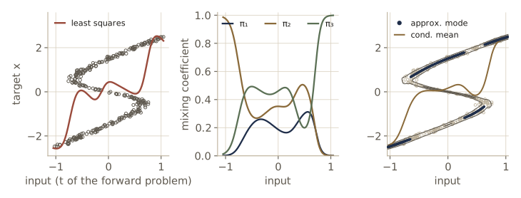
The table and figure show the whole story. Where the inverse is single-valued (inputs \(-0.9\) and \(0.9\)), one component carries most of the weight and the mode lands on the exact solution. The conditional mean is pulled away from it, because the other components keep a few percent of the mass even there; near the ends of the data the network has little evidence with which to switch them off completely, and the mean is sensitive to that leftover mass while the mode is not. Where there are three branches, the mixture places a narrow component on each, and the conditional mean and the least-squares prediction both land between branches, where no training targets are.
The approximate mode, the mean of the component with the largest mixing coefficient, always lands on a branch. At input 0.25 it agrees with the grid search. At \(-0.4\) it does not: the right branch has the largest mixing coefficient, but the middle component is less than half as wide, so its peak density is higher and the true mode is on the middle branch. Both are valid solutions of the inverse problem, which is what a controller needs; but “most probable component” and “most probable value” are different questions, and they can have different answers. Notice also how the network produces these densities. Its outputs are continuous functions of the input, yet the density switches between one and three modes; it does so by turning mixing coefficients up and down, not by making any output jump.
In practice. Mixture density networks can be finicky to train: a component can shrink its variance onto a few points and drive the likelihood up without limit. Keeping the number of components modest, putting a floor on \(\sigma_k\), and adding a little weight decay usually suffice. The same recipe of letting a network output the parameters of a distribution reappears later in the course, for example in the autoregressive and latent-variable models of modules 11 to 20.
Summary
| Idea | What it does | Key equation or property |
|---|---|---|
| Curse of dimensionality | fixed bases need exponentially many functions | \(\binom{D+M}{M}\) polynomial terms; \(5^D\) grid cells |
| High-dimensional geometry | volume and Gaussian mass move to a thin shell | shell fraction \(1 - (1-\epsilon)^D\); \(\lVert \mathbf{x} \rVert \approx \sqrt{D}\) |
| Data manifolds | real data occupy a low-dimensional curved set | few principal components, small nearest-neighbour distances |
| Multilayer network | learned basis functions, layer by layer | \(\mathbf{z}^{(l)} = h^{(l)}(\mathbf{W}^{(l)}\mathbf{z}^{(l-1)})\) |
| Universal approximation | two layers suffice in principle | existence only; width may be exponential, training may not find it |
| Activation functions | nonlinearity of the hidden units | sigmoidal saturate; ReLU family keeps slope 1 for \(a > 0\) |
| Weight-space symmetries | many weight vectors, one function | \(2^M M!\) per tanh layer; positive rescaling for ReLU |
| Depth efficiency | composition multiplies linear pieces | \(2^L\) pieces from \(2L\) ReLU units |
| Transfer and contrastive learning | reuse or learn representations | frozen features, fine-tuning; InfoNCE = cross-entropy over similarities |
| Error functions | negative log-likelihood with matched output | \(\partial E_n / \partial a_k = y_k - t_k\) |
| Mixture density network | multimodal \(p(t \mid \mathbf{x})\) | outputs set \(\pi_k, \mu_k, \sigma_k\); gradients \(\pi_k - \gamma_{nk}\) and relatives |
Ideas to carry forward:
- Fixed basis functions fail in high dimensions because they tile the whole space; neural networks succeed because they learn basis functions adapted to the low-dimensional manifold where the data live.
- Depth is not needed for expressiveness in principle, but it buys efficiency (compositions multiply) and a useful inductive bias (hierarchies of features), and it produces representations that can be reused across tasks or learned without labels.
- The error function comes from a likelihood. Pick the conditional distribution that matches the data, let the network output its parameters, and minimize the negative log-likelihood; when the distribution is multimodal, change the distribution, not the metric.
- From here on, gradients come from automatic differentiation. Module 07 is about what we do with them, and module 08 about how they are computed.
Exercises
- Use the identity \(\int_{-\infty}^{\infty} e^{-x^2/2} dx = \sqrt{2\pi}\) in each of \(D\) coordinates, and polar coordinates, to show that the unit sphere in \(D\) dimensions has surface area \(S_D = 2\pi^{D/2}/\Gamma(D/2)\) and the unit ball volume \(S_D / D\). Check the familiar values for \(D = 2\) and \(D = 3\), and check
log_radial_densityagainst a histogram of sampled radii for \(D = 50\). - Estimate by Monte Carlo the fraction of the cube \([-1, 1]^D\) that lies inside the unit ball, for \(D = 2, \dots, 12\), and compare with the exact value from exercise 1. Where does the rest of the cube’s volume go? Compute the ratio of the distance from the center to a corner and the distance to a face.
- Show that \(\tanh(a) = 2\sigma(2a) - 1\). Given a two-layer network with logistic sigmoid hidden units, construct the weights and biases of a tanh network that computes exactly the same function, and verify your construction with
two_layer. - Show that the softplus \(\zeta(a) = \ln(1 + e^a)\) satisfies \(\zeta(a) - \zeta(-a) = a\), \(\zeta'(a) = \sigma(a)\), and \(\ln\sigma(a) = -\zeta(-a)\). Then show that \(a\,\sigma(\beta a)\) tends to \(\max(0, a)\) as \(\beta \to \infty\), and plot its derivative for \(\beta = 0.5, 1, 5\) to see where it is negative.
- For a network with two hidden layers of \(M_1\) and \(M_2\) tanh units, how many equivalent weight vectors does each weight vector have? Extend the enumeration code to verify your count for \(M_1 = 2\), \(M_2 = 3\).
- Suppose each binary label was flipped with probability \(\epsilon\) before we saw it. Write down \(p(t \mid \mathbf{x})\) in terms of \(y = p(\mathcal{C}_1 \mid \mathbf{x})\), derive the error function and its derivative with respect to the output pre-activation, and check the derivative with autograd. What happens as \(\epsilon \to 1/2\)? Train a classifier on data with 20% flipped labels using both errors and compare.
- For vector targets with Gaussian noise of unknown full covariance \(\boldsymbol{\Sigma}\), write the negative log-likelihood, and show that for fixed \(\mathbf{w}\) it is minimized by the sample covariance of the residuals. Why do \(\mathbf{w}\) and \(\boldsymbol{\Sigma}\) now have to be optimized together, when with independent targets and shared variance they could be found one after the other?
- Train (with autograd and Adam) a two-layer ReLU network with \(M\) hidden units to fit the sawtooth \(g^{(4)}\) on 512 points, for \(M = 8, 16, 32\), and a network with four hidden layers of 2 ReLU units from random initialization. Which reach small error? Compare with the hand-built deep network, and discuss what this says about representation versus optimization.
- Derive the conditional mean and variance formulas for the mixture density network from the definition of the mixture. Then show that \(\gamma_{nk}\) is the posterior probability of component \(k\) given \(t_n\) and \(\mathbf{x}_n\).
- Repeat the mixture density network fit with \(K = 1, 2, 3, 5\) components and report the negative log-likelihood on a fresh test set drawn from the same generator. Where does \(K = 2\) fail? Also compute the fraction of test targets within two standard deviations \(s(\mathbf{x})\) of the conditional mean, and explain why that fraction is misleading for a multimodal density.
- In the contrastive experiment, replace the two random placements by the same placement plus independent Gaussian pixel noise (so the positive pairs no longer differ in position), train again, and evaluate the probe. Then try temperatures \(\tau = 0.05, 0.1, 0.5, 1\). Which choices matter most, and why?
- In your own words: why can a network with one hidden layer approximate any continuous function, yet deep networks are preferred in practice? Give three distinct reasons, each with an example from this module.
Going further
- C. M. Bishop and H. Bishop, Deep Learning: Foundations and Concepts, chapter 6. Exercises 6.1–6.3 (geometry of high-dimensional spaces), 6.4–6.7 (activation functions), 6.8–6.15 (error functions and their derivatives), and 6.16–6.21 (robot kinematics and mixture density networks) extend this module.
- George Cybenko, “Approximation by superpositions of a sigmoidal function”, Mathematics of Control, Signals and Systems, 1989, one of the universal approximation theorems.
- Aaron van den Oord, Yazhe Li, and Oriol Vinyals, “Representation learning with contrastive predictive coding”, 2018, which introduced the InfoNCE name; and Ting Chen, Simon Kornblith, Mohammad Norouzi, and Geoffrey Hinton, “A simple framework for contrastive learning of visual representations”, 2020, instance discrimination with augmentations and in-batch negatives.
- Ian Goodfellow, Yoshua Bengio, and Aaron Courville, Deep Learning (MIT Press, 2016), free online; chapter 6 covers feed-forward networks, activation functions, and output units, and chapter 15 representation learning.
- Intro to ML, module 05 builds the two-layer network, backpropagation, and a mixture density network from scratch in NumPy. In this course, module 07 trains networks with gradient descent and its variants, module 08 derives and implements backpropagation and automatic differentiation, and module 09 covers regularization, augmentation, and residual connections.
These notes follow the chapters of C. M. Bishop and H. Bishop, Deep Learning: Foundations and Concepts (Springer, 2024), the course text, which the authors make free to read online. The explanations, code, figures, and exercises here are written for this course; the book remains the reference, with the full derivations and many more exercises.