CSE 455/555 · Module 03 · Session 3
Maximum-Likelihood and Bayesian Parameter Estimation
Maximum likelihood and bias, Bayesian learning of Gaussian parameters, sufficient statistics, the curse of dimensionality, PCA and Fisher discriminants, EM, and hidden Markov models.
Companion reading: Duda, Hart & Stork, Pattern Classification, chapter 3, “Maximum-Likelihood and Bayesian Parameter Estimation”
By the end of this module you can
- Write down the log-likelihood of an i.i.d. sample, derive the maximum-likelihood estimates of a Gaussian’s mean and covariance, and show by derivation and by simulation that the ML variance is biased.
- Compute the posterior and the predictive density of a Gaussian mean with a Gaussian prior, in one and in d dimensions, and check the posterior against a brute-force grid.
- Run recursive (incremental) Bayesian learning on a model whose posterior is not Gaussian, and explain when the Bayesian and maximum-likelihood answers differ, what a noninformative prior is, and what the Gibbs algorithm gives up.
- State the factorization theorem, find sufficient statistics for members of the exponential family, and explain why only these few numbers need to be kept.
- Explain why adding features can hurt a classifier built from estimated parameters, show the peaking phenomenon in a simulation, count the cost of training a Gaussian classifier, and regularize covariance estimates by shrinkage.
- Derive and implement principal component analysis, Fisher’s linear discriminant, and multiple discriminant analysis, and say when each is the right projection.
- Derive the EM algorithm for a Gaussian with missing feature values, implement it, and check that the observed-data log-likelihood never decreases.
- Solve the three HMM problems — evaluation with the forward and backward algorithms, decoding with Viterbi, learning with Baum–Welch — and check the first two against brute-force enumeration of all hidden paths.
Contents
- From decision theory to estimation
- Maximum-likelihood estimation
- Bayesian estimation
- Bayesian parameter estimation: Gaussian case
- Bayesian parameter estimation: general theory
- Sufficient statistics
- Problems of dimensionality
- Component analysis and discriminants
- Expectation-maximization
- Summary
- Exercises
- Going further
In module 02 we built the optimal classifier under one large assumption: that we know the priors \(P(\omega_j)\) and the class-conditional densities \(p(\mathbf{x} \mid \omega_j)\). In practice we know neither. What we have is a training set: a finite collection of labeled samples, together with some general knowledge about the problem, for instance that each class is roughly Gaussian. This module is about turning those samples into the densities the Bayes rule needs.
The approach of this chapter of Duda, Hart & Stork (DHS from here on) is parametric: we assume each \(p(\mathbf{x} \mid \omega_j)\) has a known functional form fixed by a parameter vector \(\boldsymbol{\theta}_j\) (a mean and a covariance, say), and we estimate the parameters. There are two classical ways to do it. Maximum-likelihood estimation treats \(\boldsymbol{\theta}\) as a fixed unknown and picks the value that makes the observed data most probable. Bayesian estimation treats \(\boldsymbol{\theta}\) as a random variable with a prior distribution and uses the data to turn the prior into a posterior. We develop both, see when they agree, and see when they do not.
The second half of the module deals with the practical problems that appear as soon as parameters are estimated: too many features for too few samples (the curse of dimensionality), linear projections that reduce dimension (principal components and Fisher’s discriminant), data with missing values (the EM algorithm), and data that come as sequences (hidden Markov models). Several of these topics are derived at greater length in the Intro to ML notes, and we link to them where they help; the treatment here is self-contained and follows DHS’s notation and emphasis. The ML notes follow Bishop, who writes the transpose as \(^{\mathrm{T}}\) and classes as \(\mathcal{C}_k\); here, as in DHS, the transpose is \(^{t}\) and classes are \(\omega_j\).
The first cell sets up the libraries used throughout.
import numpy as np
from itertools import product
from scipy import stats
from scipy.special import logsumexp, ndtr
from scipy.linalg import eigh, cho_factor, cho_solve

np.set_printoptions(precision=4, suppress=True)
rng = np.random.default_rng(455)
From decision theory to estimation
Suppose we have \(c\) classes and, for each class \(\omega_j\), a set \(\mathcal{D}_j\) of samples drawn from \(p(\mathbf{x} \mid \omega_j)\). Within a set, the samples are independent draws from the same density, that class’s density; such samples are called i.i.d. (independent and identically distributed). Because we know which class produced each sample, this is supervised learning; when labels are missing the problem becomes unsupervised learning, the subject of module 10.
Estimating the priors is easy: the fraction of training samples in each class is a good estimate when the training set was collected in the same proportions as future data. The class-conditional densities are the hard part. A density is a whole function, and with many features the samples are spread thinly. The parametric assumption replaces the function with a handful of numbers. If we are willing to say that \(p(\mathbf{x} \mid \omega_j)\) is normal with mean \(\boldsymbol{\mu}_j\) and covariance \(\boldsymbol{\Sigma}_j\), then learning the density means learning \(\boldsymbol{\mu}_j\) and \(\boldsymbol{\Sigma}_j\).
We make one more simplifying assumption throughout: the parameters of different classes are functionally independent, so the samples in \(\mathcal{D}_i\) tell us nothing about \(\boldsymbol{\theta}_j\) for \(j \neq i\). Then the \(c\) estimation problems separate, and we can drop the class index and study one problem: given a set \(\mathcal{D} = \{\mathbf{x}_1, \dots, \mathbf{x}_n\}\) of \(n\) i.i.d. samples from \(p(\mathbf{x} \mid \boldsymbol{\theta})\), what can we say about \(\boldsymbol{\theta}\)?
Maximum-likelihood estimation
Maximum likelihood is the workhorse of parameter estimation. It is usually simple to compute, and as \(n\) grows its estimates converge to the true values under mild conditions.
The general principle
Because the samples are independent, the probability density of the whole data set is a product,
\[p(\mathcal{D} \mid \boldsymbol{\theta}) = \prod_{k=1}^{n} p(\mathbf{x}_k \mid \boldsymbol{\theta}).\]Seen as a function of \(\boldsymbol{\theta}\) with the data held fixed, this is the likelihood of \(\boldsymbol{\theta}\). The maximum-likelihood (ML) estimate \(\hat{\boldsymbol{\theta}}\) is the value of \(\boldsymbol{\theta}\) that maximizes it: the parameter value under which the data we actually saw were most probable. The likelihood is not a probability density over \(\boldsymbol{\theta}\); it need not integrate to one, and its area means nothing.
Products of many small numbers are awkward, both on paper and in floating point, so we work with the log-likelihood
\[l(\boldsymbol{\theta}) = \ln p(\mathcal{D} \mid \boldsymbol{\theta}) = \sum_{k=1}^{n} \ln p(\mathbf{x}_k \mid \boldsymbol{\theta}).\]The logarithm is increasing, so \(l\) and the likelihood have the same maximizer. If \(\boldsymbol{\theta} = (\theta_1, \dots, \theta_p)^t\) and \(l\) is differentiable, write \(\nabla_{\boldsymbol{\theta}} = (\partial/\partial\theta_1, \dots, \partial/\partial\theta_p)^t\) for the gradient. A set of necessary conditions for an interior maximum is
\[\nabla_{\boldsymbol{\theta}} l = \sum_{k=1}^{n} \nabla_{\boldsymbol{\theta}} \ln p(\mathbf{x}_k \mid \boldsymbol{\theta}) = \mathbf{0},\]\(p\) equations in \(p\) unknowns. A solution may be the global maximum, but it may also be a local maximum, a minimum, or a saddle point, so candidates have to be checked. And the maximum can sit on the boundary of the allowed parameter region, where the gradient need not vanish at all.
The next cell shows both situations in one dimension. For a Gaussian with known \(\sigma = 1.5\) and unknown mean, a fine grid search over \(\mu\) lands on the sample mean (we prove this below). For samples from a uniform density on \([0, \theta]\), the likelihood is \(\theta^{-n}\) when \(\theta\) is at least the largest sample and zero otherwise; its derivative \(-n\theta^{-(n+1)}\) is never zero, and the maximum sits at the edge of the region where the likelihood is positive.
def loglik_gauss_mean(x, mu_grid, sigma):
    """l(mu) = sum_k ln N(x_k | mu, sigma^2), one value per grid point."""
    sq = ((x[None, :] - mu_grid[:, None]) ** 2).sum(axis=1)
    return -0.5 * len(x) * np.log(2 * np.pi * sigma**2) - 0.5 * sq / sigma**2

x_g = rng.normal(2.0, 1.5, size=12)
mu_grid = np.linspace(-2.0, 6.0, 80001)
l_mu = loglik_gauss_mean(x_g, mu_grid, 1.5)
print(f"Gaussian: grid maximizer of l(mu) = {mu_grid[np.argmax(l_mu)]:.4f},"
      f"  sample mean = {x_g.mean():.4f}")

x_u = rng.uniform(0.0, 3.0, size=8)
th_grid = np.linspace(0.01, 6.0, 59901)
with np.errstate(divide="ignore"):
    l_th = np.where(th_grid >= x_u.max(), -len(x_u) * np.log(th_grid), -np.inf)
print(f"uniform:  grid maximizer of l(theta) = {th_grid[np.argmax(l_th)]:.4f},"
      f"  largest sample = {x_u.max():.4f}")
Gaussian: grid maximizer of l(mu) = 1.1796,  sample mean = 1.1796
uniform:  grid maximizer of l(theta) = 2.6693,  largest sample = 2.6692
The maximum a posteriori (MAP) estimate is a close relative. If we have a prior density \(p(\boldsymbol{\theta})\), MAP maximizes \(l(\boldsymbol{\theta}) + \ln p(\boldsymbol{\theta})\), the log of the posterior up to a constant; it finds the mode of the posterior. ML is MAP with a flat prior. MAP has a weakness that ML does not share: if we describe the same model with a nonlinearly transformed parameter, the posterior density changes shape and its mode moves, so the MAP answer depends on how we chose to write the parameter. We measure this effect when we discuss noninformative priors.
The Gaussian case: unknown mean
Let the samples come from \(N(\boldsymbol{\mu}, \boldsymbol{\Sigma})\) with \(\boldsymbol{\Sigma}\) known and \(\boldsymbol{\mu}\) unknown. For one sample,
\[\begin{gathered} \ln p(\mathbf{x}_k \mid \boldsymbol{\mu}) = -\frac{1}{2}\ln\left[(2\pi)^d \lvert \boldsymbol{\Sigma} \rvert\right] - \frac{1}{2}(\mathbf{x}_k - \boldsymbol{\mu})^t \boldsymbol{\Sigma}^{-1} (\mathbf{x}_k - \boldsymbol{\mu}), \\ \nabla_{\boldsymbol{\mu}} \ln p(\mathbf{x}_k \mid \boldsymbol{\mu}) = \boldsymbol{\Sigma}^{-1}(\mathbf{x}_k - \boldsymbol{\mu}). \end{gathered}\]Setting the sum of the gradients to zero gives \(\boldsymbol{\Sigma}^{-1}\sum_k(\mathbf{x}_k - \hat{\boldsymbol{\mu}}) = \mathbf{0}\), and multiplying through by \(\boldsymbol{\Sigma}\) gives
\[\hat{\boldsymbol{\mu}} = \frac{1}{n}\sum_{k=1}^{n}\mathbf{x}_k .\]The ML estimate of the mean is the sample mean, the centroid of the data cloud. The log-likelihood is a concave quadratic in \(\boldsymbol{\mu}\), so this stationary point is the global maximum.
The Gaussian case: unknown mean and covariance
Now both are unknown. Start with one dimension and write \(\theta_1 = \mu\), \(\theta_2 = \sigma^2\). Then
\[\begin{gathered} \ln p(x_k \mid \boldsymbol{\theta}) = -\frac{1}{2}\ln(2\pi\theta_2) - \frac{(x_k - \theta_1)^2}{2\theta_2}, \\ \nabla_{\boldsymbol{\theta}} \ln p(x_k \mid \boldsymbol{\theta}) = \begin{pmatrix} (x_k - \theta_1)/\theta_2 \\ -\dfrac{1}{2\theta_2} + \dfrac{(x_k - \theta_1)^2}{2\theta_2^2} \end{pmatrix}. \end{gathered}\]Summing over \(k\) and setting both components to zero, the first equation gives \(\hat{\theta}_1 = \frac{1}{n}\sum_k x_k\), and multiplying the second by \(2\hat{\theta}_2^2\) gives
\[\begin{gathered} \hat{\mu} = \frac{1}{n}\sum_{k=1}^{n} x_k, \\ \hat{\sigma}^2 = \frac{1}{n}\sum_{k=1}^{n}(x_k - \hat{\mu})^2 . \end{gathered}\]The multivariate result has the same shape:
\[\begin{gathered} \hat{\boldsymbol{\mu}} = \frac{1}{n}\sum_{k=1}^{n}\mathbf{x}_k, \\ \hat{\boldsymbol{\Sigma}} = \frac{1}{n}\sum_{k=1}^{n}(\mathbf{x}_k - \hat{\boldsymbol{\mu}})(\mathbf{x}_k - \hat{\boldsymbol{\mu}})^t . \end{gathered}\]To see where \(\hat{\boldsymbol{\Sigma}}\) comes from, write the log-likelihood in terms of the inverse covariance \(\boldsymbol{\Lambda} = \boldsymbol{\Sigma}^{-1}\) and use \(\mathbf{a}^t\boldsymbol{\Lambda}\mathbf{a} = \operatorname{tr}(\boldsymbol{\Lambda}\mathbf{a}\mathbf{a}^t)\):
\[\begin{gathered} l = \frac{n}{2}\ln\lvert \boldsymbol{\Lambda} \rvert - \frac{1}{2}\operatorname{tr}\left(\boldsymbol{\Lambda}\mathbf{M}\right) + \text{const}, \\ \mathbf{M} = \sum_{k=1}^{n}(\mathbf{x}_k - \boldsymbol{\mu})(\mathbf{x}_k - \boldsymbol{\mu})^t . \end{gathered}\]The matrix derivatives \(\partial \ln\lvert\boldsymbol{\Lambda}\rvert/\partial\boldsymbol{\Lambda} = \boldsymbol{\Lambda}^{-1}\) and \(\partial\operatorname{tr}(\boldsymbol{\Lambda}\mathbf{M})/\partial\boldsymbol{\Lambda} = \mathbf{M}\) (for symmetric matrices) give \(\frac{n}{2}\boldsymbol{\Sigma} - \frac{1}{2}\mathbf{M} = \mathbf{0}\), and with \(\boldsymbol{\mu}\) at its own optimum \(\hat{\boldsymbol{\mu}}\) this is the formula above. The ML covariance is the average of the \(n\) outer products \((\mathbf{x}_k - \hat{\boldsymbol{\mu}})(\mathbf{x}_k - \hat{\boldsymbol{\mu}})^t\), the sample version of \(\mathbb{E}[(\mathbf{x} - \boldsymbol{\mu})(\mathbf{x} - \boldsymbol{\mu})^t]\).
The code below implements both estimates and a Gaussian log-likelihood built on a Cholesky factor (no explicit inverse or determinant). It checks the log-likelihood against scipy.stats, then checks the stationarity conditions numerically: a central finite difference of \(l\) in every direction of \(\boldsymbol{\mu}\) and every symmetric direction of \(\boldsymbol{\Sigma}\) should be zero at the ML estimate, and clearly nonzero elsewhere.
def fit_gaussian_ml(X):
    """ML estimates: sample mean and the 1/n sample covariance."""
    mu = X.mean(axis=0)
    D = X - mu
    return mu, D.T @ D / len(X)

def gauss_loglik(X, mu, Sigma):
    """l = sum_k ln N(x_k | mu, Sigma), computed with a Cholesky factor."""
    L, low = cho_factor(Sigma, lower=True)
    D = X - mu
    maha = np.sum(D * cho_solve((L, low), D.T).T, axis=1)
    logdet = 2.0 * np.sum(np.log(np.diag(L)))
    n, d = X.shape
    return -0.5 * maha.sum() - 0.5 * n * (d * np.log(2 * np.pi) + logdet)

def max_slope(f, mu, Sigma, eps=1e-6):
    """Largest central-difference slope of f(mu, Sigma) along each mean coordinate
    and each symmetric covariance direction E_ij + E_ji."""
    d = len(mu)
    dirs = [(np.eye(d)[i] * eps, np.zeros((d, d))) for i in range(d)]
    for i in range(d):
        for j in range(i, d):
            E = np.zeros((d, d)); E[i, j] = E[j, i] = eps
            dirs.append((np.zeros(d), E))
    return max(abs(f(mu + dm, Sigma + dS) - f(mu - dm, Sigma - dS)) / (2 * eps)
               for dm, dS in dirs)

mu_true = np.array([1.0, -1.0, 0.5])
Sigma_true = np.array([[2.0, 0.6, 0.0],
                       [0.6, 1.0, -0.3],
                       [0.0, -0.3, 0.5]])
X3 = rng.multivariate_normal(mu_true, Sigma_true, size=200)
mu_hat, Sigma_hat = fit_gaussian_ml(X3)

l_ours = gauss_loglik(X3, mu_hat, Sigma_hat)
l_scipy = stats.multivariate_normal(mu_hat, Sigma_hat).logpdf(X3).sum()
print(f"log-likelihood: ours {l_ours:.6f}   scipy {l_scipy:.6f}")
l_X3 = lambda m, S: gauss_loglik(X3, m, S)
print(f"largest slope of l at the ML estimate:     {max_slope(l_X3, mu_hat, Sigma_hat):.2e}")
print(f"largest slope of l at the true parameters: {max_slope(l_X3, mu_true, Sigma_true):.2f}")
print("mu_hat =", mu_hat)
print("Sigma_hat =\n", Sigma_hat)
log-likelihood: ours -783.306847   scipy -783.306847
largest slope of l at the ML estimate:     5.68e-08
largest slope of l at the true parameters: 35.48
mu_hat = [ 0.9918 -0.9821  0.5079]
Sigma_hat =
 [[ 2.1194  0.5658  0.0809]
 [ 0.5658  0.7737 -0.2318]
 [ 0.0809 -0.2318  0.4899]]
The slopes vanish (to finite-difference accuracy) at \((\hat{\boldsymbol{\mu}}, \hat{\boldsymbol{\Sigma}})\) and do not vanish at the true parameters: the data “prefer” the ML estimate to the truth, as they must.
Bias
An estimator is unbiased if its expected value, averaged over all data sets of size \(n\), equals the true parameter. The sample mean is unbiased. The ML variance is not. To see why, split each deviation from the sample mean \(\bar{x}\) into a deviation from the true mean and a correction:
\[\sum_{k=1}^{n}(x_k - \bar{x})^2 = \sum_{k=1}^{n}(x_k - \mu)^2 - n(\bar{x} - \mu)^2 .\]Taking expectations, the first sum contributes \(n\sigma^2\) and the second \(n \cdot \sigma^2/n = \sigma^2\), because the variance of \(\bar{x}\) is \(\sigma^2/n\). So
\[\mathbb{E}\left[\frac{1}{n}\sum_{k=1}^{n}(x_k - \bar{x})^2\right] = \frac{n-1}{n}\,\sigma^2 \neq \sigma^2 .\]The sample mean sits closer to the data than the true mean does (it was chosen to), so deviations measured from it are too small on average. The extreme case makes this obvious: with \(n = 1\), the ML variance is always zero. The same argument applied to outer products shows that \(\hat{\boldsymbol{\Sigma}}\) is biased by the same factor, and that the sample covariance
\[\mathbf{C} = \frac{1}{n-1}\sum_{k=1}^{n}(\mathbf{x}_k - \hat{\boldsymbol{\mu}})(\mathbf{x}_k - \hat{\boldsymbol{\mu}})^t\]is unbiased. DHS call an estimator that is unbiased for every distribution, like \(\mathbf{C}\), absolutely unbiased, and one whose bias disappears as \(n \to \infty\), like \(\hat{\boldsymbol{\Sigma}} = \frac{n-1}{n}\mathbf{C}\), asymptotically unbiased.
A simulation makes the bias visible. We draw many data sets of size \(n\) from \(N(0, 4)\), compute both estimates on each, and average. We also record each estimator’s mean squared error around the true value 4.
rng_b = np.random.default_rng(3)
sigma2 = 4.0
print("  n   mean of ML var   (n-1)/n * 4   mean of C   MSE of ML var   MSE of C")
for n in [2, 3, 5, 10, 50]:
    x = rng_b.normal(0.0, np.sqrt(sigma2), size=(50_000, n))   # 50,000 data sets
    ss = ((x - x.mean(axis=1, keepdims=True)) ** 2).sum(axis=1)
    v_ml, v_c = ss / n, ss / (n - 1)
    print(f"{n:3d}   {v_ml.mean():14.4f}   {(n - 1) / n * sigma2:11.4f}   {v_c.mean():9.4f}"
          f"   {np.mean((v_ml - sigma2) ** 2):13.4f}   {np.mean((v_c - sigma2) ** 2):8.4f}")
  n   mean of ML var   (n-1)/n * 4   mean of C   MSE of ML var   MSE of C
  2           2.0085        2.0000      4.0170         12.0812    32.4610
  3           2.6738        2.6667      4.0107          8.8980    16.0632
  5           3.2042        3.2000      4.0052          5.7224     7.9517
 10           3.5973        3.6000      3.9970          3.0441     3.5580
 50           3.9160        3.9200      3.9960          0.6348     0.6537
The averages of the ML variance track \(\frac{n-1}{n}\cdot 4\), and the averages of \(\mathbf{C}\) sit at 4, within Monte Carlo error. The last two columns carry a second lesson: the biased ML estimator has the smaller mean squared error for every \(n\), because dividing by \(n\) instead of \(n - 1\) shrinks the estimate and lowers its variance by more than the bias costs. Neither estimator is “the correct one”; they optimize different things. What we really want is the estimate that gives the best classifier, and that question has no general answer; we return to it with Bayesian methods below and with bias and variance in module 09.
Watch out. Maximum likelihood finds the best parameters within the assumed model. If the model is wrong — say the data are not Gaussian at all — the ML parameters need not give the best classifier even among classifiers of the assumed form. DHS Problem 7 builds an example where the difference is large. Reliable knowledge of the model’s form matters as much as the estimation method.
Bayesian estimation
The Bayesian approach changes the question. Instead of one best value of \(\boldsymbol{\theta}\), it asks for a whole distribution: what we believed about \(\boldsymbol{\theta}\) before the data (the prior), updated by the data into the posterior. The final answer is a density for \(\mathbf{x}\) that averages over the parameter values we still consider plausible.
The class-conditional densities
The posterior probabilities of the classes are what the Bayes classifier needs. With the training data made explicit, Bayes’ formula reads
\[P(\omega_i \mid \mathbf{x}, \mathcal{D}) = \frac{p(\mathbf{x} \mid \omega_i, \mathcal{D})\,P(\omega_i \mid \mathcal{D})}{\sum_{j=1}^{c} p(\mathbf{x} \mid \omega_j, \mathcal{D})\,P(\omega_j \mid \mathcal{D})} .\]Two simplifications, the same as before, bring this down to size. The priors are known or trivially estimated, so \(P(\omega_i \mid \mathcal{D}) = P(\omega_i)\). And the training data split by class, with each subset \(\mathcal{D}_i\) informative only about its own class, so \(p(\mathbf{x} \mid \omega_i, \mathcal{D}) = p(\mathbf{x} \mid \omega_i, \mathcal{D}_i)\). Then
\[P(\omega_i \mid \mathbf{x}, \mathcal{D}) = \frac{p(\mathbf{x} \mid \omega_i, \mathcal{D}_i)\,P(\omega_i)}{\sum_{j=1}^{c} p(\mathbf{x} \mid \omega_j, \mathcal{D}_j)\,P(\omega_j)},\]and each class poses the same problem: from a set \(\mathcal{D}\) of samples drawn from an unknown density \(p(\mathbf{x})\), compute \(p(\mathbf{x} \mid \mathcal{D})\), our best estimate of that density given the data. Computing it is the core task of Bayesian learning.
The parameter distribution
We assume \(p(\mathbf{x})\) has a known form \(p(\mathbf{x} \mid \boldsymbol{\theta})\) with \(\boldsymbol{\theta}\) unknown, and that what we know about \(\boldsymbol{\theta}\) before seeing data is captured by a known prior \(p(\boldsymbol{\theta})\). Marginalizing over the parameter,
\[p(\mathbf{x} \mid \mathcal{D}) = \int p(\mathbf{x}, \boldsymbol{\theta} \mid \mathcal{D})\,d\boldsymbol{\theta} = \int p(\mathbf{x} \mid \boldsymbol{\theta})\,p(\boldsymbol{\theta} \mid \mathcal{D})\,d\boldsymbol{\theta} .\]The second step uses the fact that a new \(\mathbf{x}\) is drawn independently of the training set once \(\boldsymbol{\theta}\) is fixed, so \(p(\mathbf{x} \mid \boldsymbol{\theta}, \mathcal{D}) = p(\mathbf{x} \mid \boldsymbol{\theta})\).
Result. The predictive density is the model density averaged over the posterior:
\[p(\mathbf{x} \mid \mathcal{D}) = \int p(\mathbf{x} \mid \boldsymbol{\theta})\,p(\boldsymbol{\theta} \mid \mathcal{D})\,d\boldsymbol{\theta}.\]The data influence the classifier only through the posterior \(p(\boldsymbol{\theta} \mid \mathcal{D})\).
If the posterior is sharply peaked at some \(\hat{\boldsymbol{\theta}}\), the integral is close to \(p(\mathbf{x} \mid \hat{\boldsymbol{\theta}})\), and we are back to plugging in a point estimate. When the posterior is broad, the integral averages many plausible densities, and the result can differ from any single member of the family. When the integral has no closed form it can be approximated numerically, for instance by Monte Carlo: draw parameter values from the posterior and average \(p(\mathbf{x} \mid \boldsymbol{\theta})\) over them.
Bayesian parameter estimation: Gaussian case
The Gaussian with unknown mean is the case where every step can be done in closed form, and it shows the typical behavior of Bayesian learning clearly.
The univariate case: the posterior of the mean
Let \(p(x \mid \mu) = N(\mu, \sigma^2)\) with \(\sigma^2\) known, and let the prior on the mean be \(p(\mu) = N(\mu_0, \sigma_0^2)\) with \(\mu_0\) and \(\sigma_0^2\) known. Informally, \(\mu_0\) is our best guess before seeing data and \(\sigma_0\) says how far off we think that guess might be. What matters most is not that the prior is Gaussian but that it is known: it is part of the model, chosen before the data arrive.
By Bayes’ formula, with \(\alpha\) a normalizing constant that does not depend on \(\mu\),
\[\begin{aligned} p(\mu \mid \mathcal{D}) &= \alpha \prod_{k=1}^{n} p(x_k \mid \mu)\,p(\mu) \\ &= \alpha' \exp\left[-\frac{1}{2}\left(\sum_{k=1}^{n}\frac{(x_k - \mu)^2}{\sigma^2} + \frac{(\mu - \mu_0)^2}{\sigma_0^2}\right)\right] \\ &= \alpha'' \exp\left[-\frac{1}{2}\left(\left(\frac{n}{\sigma^2} + \frac{1}{\sigma_0^2}\right)\mu^2 - 2\left(\frac{n\hat{\mu}_n}{\sigma^2} + \frac{\mu_0}{\sigma_0^2}\right)\mu\right)\right], \end{aligned}\]where \(\hat{\mu}_n = \frac{1}{n}\sum_k x_k\) is the sample mean and every factor free of \(\mu\) has been absorbed into the constants. The exponent is quadratic in \(\mu\), so the posterior is again normal, \(p(\mu \mid \mathcal{D}) = N(\mu_n, \sigma_n^2)\). Matching the coefficient of \(\mu^2\) and of \(\mu\) with those of \(-\frac{1}{2}(\mu - \mu_n)^2/\sigma_n^2\) gives
\[\begin{gathered} \frac{1}{\sigma_n^2} = \frac{n}{\sigma^2} + \frac{1}{\sigma_0^2}, \\ \frac{\mu_n}{\sigma_n^2} = \frac{n}{\sigma^2}\hat{\mu}_n + \frac{\mu_0}{\sigma_0^2}. \end{gathered}\]Precisions (inverse variances) add, and the posterior mean is a precision-weighted average. Solving,
\[\begin{gathered} \mu_n = \frac{n\sigma_0^2}{n\sigma_0^2 + \sigma^2}\,\hat{\mu}_n + \frac{\sigma^2}{n\sigma_0^2 + \sigma^2}\,\mu_0, \\ \sigma_n^2 = \frac{\sigma_0^2\sigma^2}{n\sigma_0^2 + \sigma^2}. \end{gathered}\]A prior that, like this one, produces a posterior of the same family is a conjugate prior; DHS say the posterior is a reproducing density. The formulas say three things:
- \(\mu_n\) always lies between the prior guess \(\mu_0\) and the sample mean, with weights that are nonnegative and sum to one. As \(n\) grows the weight on the sample mean goes to one.
- \(\sigma_n^2\) decreases monotonically with \(n\) and behaves like \(\sigma^2/n\) for large \(n\). Each new sample makes us more certain, and the posterior tends to a spike at the true mean. This sharpening is what DHS call Bayesian learning.
- The balance between prior and data is set by the ratio \(\sigma^2/\sigma_0^2\), which DHS call the dogmatism. With \(\sigma_0 \to 0\) the prior is so confident that no amount of data moves \(\mu_n\) from \(\mu_0\); with \(\sigma_0 \to \infty\) the prior is ignored and \(\mu_n = \hat{\mu}_n\). Any finite dogmatism is eventually overwhelmed by data.
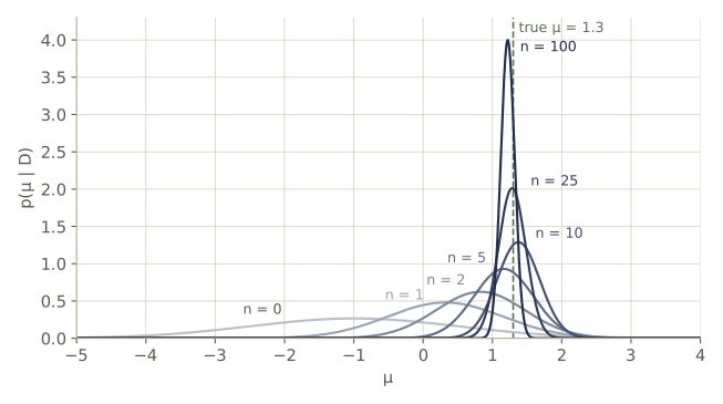
The code computes the posterior for growing \(n\) on one stream of data from a class whose true mean is 1.3, with \(\sigma = 1\) and a prior \(N(-1, 1.5^2)\) that is deliberately off target. It also runs the update one sample at a time, using each posterior as the prior for the next sample, and compares with the batch formula.
def posterior_mean_known_var(x, sigma2, mu0, sigma02):
    """p(mu | D) = N(mu_n, sigma_n^2) for x_k ~ N(mu, sigma2), prior N(mu0, sigma02)."""
    n = len(x)
    s = np.sum(x)
    sigma_n2 = 1.0 / (n / sigma2 + 1.0 / sigma02)        # precisions add
    mu_n = sigma_n2 * (s / sigma2 + mu0 / sigma02)       # precision-weighted average
    return mu_n, sigma_n2

sigma2_b, mu0_b, sigma02_b = 1.0, -1.0, 1.5**2
x_stream = np.random.default_rng(31).normal(1.3, 1.0, size=100)

print("   n   sample mean    mu_n    sigma_n   weight on sample mean")
for n in [0, 1, 2, 5, 10, 25, 100]:
    mu_n, s_n2 = posterior_mean_known_var(x_stream[:n], sigma2_b, mu0_b, sigma02_b)
    xbar = x_stream[:n].mean() if n > 0 else float("nan")
    w = n * sigma02_b / (n * sigma02_b + sigma2_b)
    print(f"{n:4d}   {xbar:11.4f}  {mu_n:7.4f}  {np.sqrt(s_n2):8.4f}   {w:10.4f}")

m, v = mu0_b, sigma02_b                  # sequential: yesterday's posterior is today's prior
for xk in x_stream:
    m, v = posterior_mean_known_var(np.array([xk]), sigma2_b, m, v)
mu_batch, v_batch = posterior_mean_known_var(x_stream, sigma2_b, mu0_b, sigma02_b)
print(f"one at a time: mu = {m:.10f}, var = {v:.10f}")
print(f"batch:         mu = {mu_batch:.10f}, var = {v_batch:.10f}")
   n   sample mean    mu_n    sigma_n   weight on sample mean
   0           nan  -1.0000    1.5000       0.0000
   1        0.9047   0.3186    0.8321       0.6923
   2        1.2343   0.8281    0.6396       0.8182
   5        1.3542   1.1621    0.4286       0.9184
  10        1.4806   1.3750    0.3094       0.9574
  25        1.3245   1.2839    0.1982       0.9825
 100        1.2305   1.2207    0.0998       0.9956
one at a time: mu = 1.2206648759, var = 0.0099557522
batch:         mu = 1.2206648759, var = 0.0099557522
A single sample already pulls the posterior mean about 70% of the way from the prior guess toward the data, because here the prior is broader than the noise (\(\sigma_0 = 1.5 > \sigma = 1\)). By \(n = 100\) the weight on the sample mean is above 0.99 and \(\sigma_n\) is essentially \(\sigma/\sqrt{n} = 0.1\). Updating one sample at a time gives the batch posterior to every printed digit, as it must: multiplying in the likelihood factors one by one or all at once is the same product.
The univariate case: the predictive density
With the posterior in hand, the predictive density is
\[p(x \mid \mathcal{D}) = \int p(x \mid \mu)\,p(\mu \mid \mathcal{D})\,d\mu = \int N(x \mid \mu, \sigma^2)\,N(\mu \mid \mu_n, \sigma_n^2)\,d\mu .\]The integral can be done by completing the square in \(\mu\), but there is a shorter route. Under the model, a new \(x\) is \(\mu + \varepsilon\), where \(\mu\) follows the posterior \(N(\mu_n, \sigma_n^2)\) and \(\varepsilon \sim N(0, \sigma^2)\) is independent noise. A sum of independent Gaussians is Gaussian with added means and added variances, so
\[p(x \mid \mathcal{D}) = N(\mu_n,\; \sigma^2 + \sigma_n^2).\]Compared with plugging in a point estimate, the Bayesian answer uses \(\mu_n\) as the mean and widens the density by \(\sigma_n^2\), the remaining uncertainty about \(\mu\). As \(n\) grows, \(\sigma_n^2 \to 0\) and the two answers merge. We check the formula by doing the integral numerically on a fine grid of \(\mu\) values, after 5 samples.
mu_n5, s_n5 = posterior_mean_known_var(x_stream[:5], sigma2_b, mu0_b, sigma02_b)
mu_g = np.linspace(mu_n5 - 10, mu_n5 + 10, 20001)
post_g = stats.norm(mu_n5, np.sqrt(s_n5)).pdf(mu_g)
for x0 in [-1.0, 0.5, 2.0, 4.0]:
    integrand = stats.norm(mu_g, np.sqrt(sigma2_b)).pdf(x0) * post_g
    numeric = np.trapezoid(integrand, mu_g)
    closed = stats.norm(mu_n5, np.sqrt(sigma2_b + s_n5)).pdf(x0)
    print(f"x = {x0:4.1f}:  integral {numeric:.8f}   N(mu_n, sigma^2 + sigma_n^2)"
          f" {closed:.8f}")
x = -1.0:  integral 0.05090292   N(mu_n, sigma^2 + sigma_n^2) 0.05090292
x =  0.5:  integral 0.30470630   N(mu_n, sigma^2 + sigma_n^2) 0.30470630
x =  2.0:  integral 0.27257514   N(mu_n, sigma^2 + sigma_n^2) 0.27257514
x =  4.0:  integral 0.01221224   N(mu_n, sigma^2 + sigma_n^2) 0.01221224
The numerical integral and the closed form agree to all eight printed digits.
The multivariate case
In \(d\) dimensions, let \(p(\mathbf{x} \mid \boldsymbol{\mu}) = N(\boldsymbol{\mu}, \boldsymbol{\Sigma})\) with \(\boldsymbol{\Sigma}\) known, and the prior \(p(\boldsymbol{\mu}) = N(\boldsymbol{\mu}_0, \boldsymbol{\Sigma}_0)\). Collecting the terms of the log posterior that depend on \(\boldsymbol{\mu}\),
\[\begin{aligned} \ln p(\boldsymbol{\mu} \mid \mathcal{D}) &= -\frac{1}{2}\sum_{k=1}^{n}(\mathbf{x}_k - \boldsymbol{\mu})^t\boldsymbol{\Sigma}^{-1}(\mathbf{x}_k - \boldsymbol{\mu}) - \frac{1}{2}(\boldsymbol{\mu} - \boldsymbol{\mu}_0)^t\boldsymbol{\Sigma}_0^{-1}(\boldsymbol{\mu} - \boldsymbol{\mu}_0) + \text{const} \\ &= -\frac{1}{2}\boldsymbol{\mu}^t\left(n\boldsymbol{\Sigma}^{-1} + \boldsymbol{\Sigma}_0^{-1}\right)\boldsymbol{\mu} + \boldsymbol{\mu}^t\left(n\boldsymbol{\Sigma}^{-1}\hat{\boldsymbol{\mu}}_n + \boldsymbol{\Sigma}_0^{-1}\boldsymbol{\mu}_0\right) + \text{const}. \end{aligned}\]Matching this with \(-\frac{1}{2}(\boldsymbol{\mu} - \boldsymbol{\mu}_n)^t\boldsymbol{\Sigma}_n^{-1}(\boldsymbol{\mu} - \boldsymbol{\mu}_n)\), the posterior is \(N(\boldsymbol{\mu}_n, \boldsymbol{\Sigma}_n)\) with
\[\begin{gathered} \boldsymbol{\Sigma}_n^{-1} = n\boldsymbol{\Sigma}^{-1} + \boldsymbol{\Sigma}_0^{-1}, \\ \boldsymbol{\Sigma}_n^{-1}\boldsymbol{\mu}_n = n\boldsymbol{\Sigma}^{-1}\hat{\boldsymbol{\mu}}_n + \boldsymbol{\Sigma}_0^{-1}\boldsymbol{\mu}_0 , \end{gathered}\]the exact analogues of the univariate formulas. To solve them without inverting three matrices, use the identity \((\mathbf{A}^{-1} + \mathbf{B}^{-1})^{-1} = \mathbf{A}(\mathbf{A} + \mathbf{B})^{-1}\mathbf{B} = \mathbf{B}(\mathbf{A} + \mathbf{B})^{-1}\mathbf{A}\), valid for nonsingular \(d \times d\) matrices, with \(\mathbf{A} = \boldsymbol{\Sigma}_0\) and \(\mathbf{B} = \frac{1}{n}\boldsymbol{\Sigma}\):
\[\begin{gathered} \boldsymbol{\Sigma}_n = \boldsymbol{\Sigma}_0\left(\boldsymbol{\Sigma}_0 + \tfrac{1}{n}\boldsymbol{\Sigma}\right)^{-1}\tfrac{1}{n}\boldsymbol{\Sigma}, \\ \boldsymbol{\mu}_n = \boldsymbol{\Sigma}_0\left(\boldsymbol{\Sigma}_0 + \tfrac{1}{n}\boldsymbol{\Sigma}\right)^{-1}\hat{\boldsymbol{\mu}}_n + \tfrac{1}{n}\boldsymbol{\Sigma}\left(\boldsymbol{\Sigma}_0 + \tfrac{1}{n}\boldsymbol{\Sigma}\right)^{-1}\boldsymbol{\mu}_0 . \end{gathered}\](Multiply \(\boldsymbol{\Sigma}_n\) by \(n\boldsymbol{\Sigma}^{-1}\) with the first form of the identity and by \(\boldsymbol{\Sigma}_0^{-1}\) with the second.) Again \(\boldsymbol{\mu}_n\) is a matrix-weighted combination of the sample mean and the prior mean. The predictive density follows from the same sum-of-independent-Gaussians argument: \(\mathbf{x} = \boldsymbol{\mu} + \boldsymbol{\varepsilon}\) with \(\boldsymbol{\mu} \sim N(\boldsymbol{\mu}_n, \boldsymbol{\Sigma}_n)\) and \(\boldsymbol{\varepsilon} \sim N(\mathbf{0}, \boldsymbol{\Sigma})\), so
\[p(\mathbf{x} \mid \mathcal{D}) = N(\boldsymbol{\mu}_n,\; \boldsymbol{\Sigma} + \boldsymbol{\Sigma}_n).\]The Gaussian identities behind these steps are collected in Intro to ML, module 02, which also treats unknown covariances with the Wishart prior.
The code implements the closed form, checks it against the precision form, and checks the predictive covariance by sampling \(\boldsymbol{\mu}\) from the posterior and then \(\mathbf{x}\) given \(\boldsymbol{\mu}\).
def posterior_mean_known_cov(X, Sigma, mu0, Sigma0):
    """p(mu | D) = N(mu_n, Sigma_n) for x_k ~ N(mu, Sigma), prior N(mu0, Sigma0)."""
    n = len(X)
    mu_hat = X.mean(axis=0)
    A = Sigma0 + Sigma / n
    mu_n = Sigma0 @ np.linalg.solve(A, mu_hat) + (Sigma / n) @ np.linalg.solve(A, mu0)
    Sigma_n = Sigma0 @ np.linalg.solve(A, Sigma / n)
    return mu_n, (Sigma_n + Sigma_n.T) / 2           # symmetrize rounding error

Sigma_k = np.array([[1.0, 0.5], [0.5, 2.0]])          # known covariance
mu0_k, Sigma0_k = np.zeros(2), np.array([[4.0, -1.0], [-1.0, 1.0]])
X2 = rng.multivariate_normal([1.5, -0.5], Sigma_k, size=8)
mu_n2, Sigma_n2 = posterior_mean_known_cov(X2, Sigma_k, mu0_k, Sigma0_k)

# precision form, with explicit inverses only as a check
P_n = 8 * np.linalg.inv(Sigma_k) + np.linalg.inv(Sigma0_k)
rhs = 8 * np.linalg.solve(Sigma_k, X2.mean(0)) + np.linalg.solve(Sigma0_k, mu0_k)
mu_prec = np.linalg.solve(P_n, rhs)
print("mu_n  (closed form) =", mu_n2, "  (precision form) =", mu_prec)
print(f"max |Sigma_n - inv(precision)| = {np.abs(Sigma_n2 - np.linalg.inv(P_n)).max():.1e}")

mus = rng.multivariate_normal(mu_n2, Sigma_n2, size=400_000)
xs = mus + rng.multivariate_normal(np.zeros(2), Sigma_k, size=400_000)
print("Sigma + Sigma_n =\n", Sigma_k + Sigma_n2)
print("sample covariance of predictive draws =\n", np.cov(xs.T))
mu_n  (closed form) = [ 1.5146 -0.9117]   (precision form) = [ 1.5146 -0.9117]
max |Sigma_n - inv(precision)| = 2.8e-17
Sigma + Sigma_n =
 [[1.1132 0.5374]
 [0.5374 2.1817]]
sample covariance of predictive draws =
 [[1.1108 0.5369]
 [0.5369 2.1827]]
The two forms of \(\boldsymbol{\mu}_n\) and \(\boldsymbol{\Sigma}_n\) agree to rounding error, and the covariance of the simulated predictive draws matches \(\boldsymbol{\Sigma} + \boldsymbol{\Sigma}_n\) to within Monte Carlo error.
As a last check on the algebra, we verify the posterior by brute force in one dimension, with no conjugacy used at all: evaluate prior times likelihood on a fine grid of \(\mu\) values, normalize numerically, and compute the mean and variance of the resulting density.
x_1d = rng.normal(0.7, 2.0, size=6)                  # sigma = 2 known
Sig, mu0_1, Sig0 = np.array([[4.0]]), np.array([3.0]), np.array([[0.5]])
mu_n1, Sig_n1 = posterior_mean_known_cov(x_1d[:, None], Sig, mu0_1, Sig0)

grid = np.linspace(-6, 9, 30001)
log_post = (stats.norm(grid[:, None], 2.0).logpdf(x_1d[None, :]).sum(axis=1)
            + stats.norm(3.0, np.sqrt(0.5)).logpdf(grid))
post = np.exp(log_post - log_post.max())
post /= np.trapezoid(post, grid)
m_grid = np.trapezoid(grid * post, grid)
v_grid = np.trapezoid((grid - m_grid) ** 2 * post, grid)
print(f"grid:        mean {m_grid:.6f}   variance {v_grid:.6f}")
print(f"closed form: mean {mu_n1[0]:.6f}   variance {Sig_n1[0, 0]:.6f}")
grid:        mean 2.029850   variance 0.285714
closed form: mean 2.029850   variance 0.285714
Bayesian parameter estimation: general theory
Nothing in the Bayesian recipe depended on Gaussians. The general version rests on three assumptions:
- the form of \(p(\mathbf{x} \mid \boldsymbol{\theta})\) is known, but \(\boldsymbol{\theta}\) is not;
- what we know about \(\boldsymbol{\theta}\) before seeing data is expressed by a known prior \(p(\boldsymbol{\theta})\);
- the rest of what we know is in \(n\) samples drawn independently from the unknown \(p(\mathbf{x})\).
The solution has three lines:
\[\begin{gathered} p(\mathbf{x} \mid \mathcal{D}) = \int p(\mathbf{x} \mid \boldsymbol{\theta})\,p(\boldsymbol{\theta} \mid \mathcal{D})\,d\boldsymbol{\theta}, \\ p(\boldsymbol{\theta} \mid \mathcal{D}) = \frac{p(\mathcal{D} \mid \boldsymbol{\theta})\,p(\boldsymbol{\theta})}{\int p(\mathcal{D} \mid \boldsymbol{\theta})\,p(\boldsymbol{\theta})\,d\boldsymbol{\theta}}, \\ p(\mathcal{D} \mid \boldsymbol{\theta}) = \prod_{k=1}^{n} p(\mathbf{x}_k \mid \boldsymbol{\theta}). \end{gathered}\]Its relation to maximum likelihood is visible in the middle formula. If the likelihood has a sharp peak at \(\hat{\boldsymbol{\theta}}\) and the prior is nonzero and roughly constant near that peak, the posterior peaks at the same place, and \(p(\mathbf{x} \mid \mathcal{D}) \approx p(\mathbf{x} \mid \hat{\boldsymbol{\theta}})\). With plenty of data the two methods agree; the Bayesian recipe tells us what to do when they do not.
Recursive Bayesian learning
Write \(\mathcal{D}^n = \{\mathbf{x}_1, \dots, \mathbf{x}_n\}\) for the first \(n\) samples. Because the likelihood is a product, \(p(\mathcal{D}^n \mid \boldsymbol{\theta}) = p(\mathbf{x}_n \mid \boldsymbol{\theta})\,p(\mathcal{D}^{n-1} \mid \boldsymbol{\theta})\), and substituting into Bayes’ formula gives a recursion:
\[\begin{gathered} p(\boldsymbol{\theta} \mid \mathcal{D}^n) = \frac{p(\mathbf{x}_n \mid \boldsymbol{\theta})\,p(\boldsymbol{\theta} \mid \mathcal{D}^{n-1})}{\int p(\mathbf{x}_n \mid \boldsymbol{\theta})\,p(\boldsymbol{\theta} \mid \mathcal{D}^{n-1})\,d\boldsymbol{\theta}}, \\ p(\boldsymbol{\theta} \mid \mathcal{D}^0) = p(\boldsymbol{\theta}). \end{gathered}\]Each posterior becomes the prior for the next sample. This is recursive Bayes learning, an example of incremental (or on-line) learning, where the model is updated as data arrive instead of waiting for the full training set. The result does not depend on the order of the samples, since the product in the likelihood does not. In general the recursion needs the whole previous posterior, which may take as much memory as the data; for some models the posterior is fixed by a few numbers (the sufficient statistics of the next section), and only those need to be carried forward. We did exactly that for the Gaussian mean, where \((\mu_n, \sigma_n^2)\) was all we kept.
A uniform example. Let the samples come from a uniform density on \([0, \theta]\), so \(p(x \mid \theta) = 1/\theta\) for \(0 \le x \le \theta\) and zero otherwise. Before any data we know only that \(0 < \theta \le 5\), and we take the prior to be flat on that interval. Each sample \(x_k\) multiplies the posterior by \(1/\theta\) and sets it to zero for \(\theta < x_k\). After \(n\) samples with largest value \(m_n = \max_k x_k\),
\[p(\theta \mid \mathcal{D}^n) = \frac{\theta^{-n}}{Z_n} \quad \text{for } m_n \le \theta \le 5, \qquad Z_n = \int_{m_n}^{5}\theta^{-n}\,d\theta,\]and zero elsewhere. The posterior is not a member of any named family and it is lopsided: it jumps up at \(m_n\) and decays toward 5. The ML estimate is \(\hat{\theta} = m_n\), the left edge of the posterior. The predictive density is
\[\begin{gathered} p(x \mid \mathcal{D}^n) = \int_{\max(x, m_n)}^{5}\frac{1}{\theta}\,\frac{\theta^{-n}}{Z_n}\,d\theta = \frac{a^{-n} - 5^{-n}}{n Z_n}, \\ a = \max(x, m_n), \end{gathered}\]which is flat for \(0 \le x \le m_n\) and then falls smoothly to zero at 5. It is not a uniform density, so the Bayesian answer lies outside the model family we started with.
The code draws 8 samples from a uniform density with \(\theta = 3.2\), runs the recursion on a grid of \(\theta\) values one sample at a time, and compares each posterior with the closed form. Then it compares the predictive density from the formula with a numerical integral, and measures how much probability the Bayesian answer places beyond the largest sample, where the ML density is zero.
theta_max = 5.0
x_unif = np.random.default_rng(8).uniform(0.0, 3.2, size=8)
print("samples:", np.round(x_unif, 3))

th = np.linspace(1e-3, theta_max, 50_000)
post = np.ones_like(th) / theta_max                    # flat prior on (0, 5]
for n, xk in enumerate(x_unif, start=1):
    post = post * np.where(th >= xk, 1.0 / th, 0.0)    # times p(x_n | theta)
    post /= np.trapezoid(post, th)                     # renormalize
    m_n = x_unif[:n].max()
    closed = np.where(th >= m_n, th ** (-n), 0.0)
    closed /= np.trapezoid(closed, th)
    if n in (1, 2, 3, 8):
        print(f"n = {n}: max sample {m_n:.3f}, posterior mode {th[np.argmax(post)]:.3f},"
              f" posterior mean {np.trapezoid(th * post, th):.3f},"
              f" max |grid - closed form| = {np.abs(post - closed).max():.1e}")

def predictive_uniform(x, data, theta_max=5.0):
    """p(x | D) for the uniform model with a flat prior on (0, theta_max]."""
    n, m = len(data), data.max()
    Z = np.log(theta_max / m) if n == 1 else (m ** (1 - n) - theta_max ** (1 - n)) / (n - 1)
    a = np.maximum(x, m)
    return np.where(x <= theta_max, (a ** (-n) - theta_max ** (-n)) / (n * Z), 0.0)

xq = np.array([0.5, 2.0, 3.5, 4.5])
numeric = [np.trapezoid(np.where(th >= x0, 1 / th, 0) * post, th) for x0 in xq]
print("predictive, formula:", predictive_uniform(xq, x_unif))
print("predictive, numeric:", np.array(numeric))
xx = np.linspace(0, theta_max, 200_001)
p_x = predictive_uniform(xx, x_unif)
m8 = x_unif.max()
print(f"total mass {np.trapezoid(p_x, xx):.4f};  mass above the largest sample"
      f" {np.trapezoid(np.where(xx > m8, p_x, 0), xx):.4f};  ML density there: 0")
samples: [1.046 3.159 1.02  2.523 2.784 1.251 1.401 1.193]
n = 1: max sample 1.046, posterior mode 1.046, posterior mean 2.528, max |grid - closed form| = 2.2e-16
n = 2: max sample 3.159, posterior mode 3.159, posterior mean 3.940, max |grid - closed form| = 4.4e-16
n = 3: max sample 3.159, posterior mode 3.159, posterior mean 3.872, max |grid - closed form| = 6.7e-16
n = 8: max sample 3.159, posterior mode 3.159, posterior mean 3.596, max |grid - closed form| = 2.7e-15
predictive, formula: [0.2812 0.2812 0.1198 0.0097]
predictive, numeric: [0.2812 0.2812 0.1198 0.0097]
total mass 1.0000;  mass above the largest sample 0.1115;  ML density there: 0
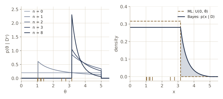
The grid recursion reproduces the closed form, the posterior mode is exactly the largest sample (the ML estimate), and the posterior mean lies to its right. The predictive density puts about 11% of its probability above the largest observed value, where the ML density is zero. That tail is the prior speaking: with eight samples the data have not yet ruled out values of \(\theta\) up to 5. Notice also what happened between \(n = 2\) and \(n = 3\): the third sample was below the current maximum, so the ML estimate did not move, but the posterior mean did.
For most well-behaved models the sequence of posteriors converges to a spike at the true parameter. Roughly, this requires that only one value of \(\boldsymbol{\theta}\) produce the true density; such a model is identifiable. When several parameter values give the same \(p(\mathbf{x} \mid \boldsymbol{\theta})\), the posterior can keep several peaks forever, but the predictive density still converges, because the integral averages densities that are all the same. Identifiability becomes a real problem in unsupervised learning (module 10), where swapping the labels of two mixture components gives the same density.
When do maximum-likelihood and Bayes methods differ?
With a reasonable prior (one that does not rule out the truth), the two methods agree in the limit of infinite data. With finite data they can differ, and several considerations bear on which to prefer.
- Computation. ML needs calculus or a numerical search; Bayes needs integrals over the parameter space, which are often high-dimensional and hard. This usually favors ML.
- Interpretability. ML returns one model from the family the designer chose and understands. The Bayesian predictive density is an average of many models and may not belong to the family at all, as in the uniform example.
- Confidence in the prior. Bayes uses more information than ML: the whole shape of the posterior, not just its peak. When the prior is sound, this information helps. When the posterior is broad or asymmetric, as it was for the uniform model, the two predictive densities differ the most. In the uniform example a new sample below the current maximum does not change the ML estimate at all, but it still sharpens the posterior.
Once the classifier is built, its errors come from three sources:
| Source of error | What causes it | Can more data remove it? |
|---|---|---|
| Bayes (indistinguishability) error | the class densities overlap | no; it is a property of the problem |
| Model error | the assumed form of \(p(\mathbf{x} \mid \omega_j, \boldsymbol{\theta})\) is wrong | no; only a better model family |
| Estimation error | parameters estimated from a finite sample | yes |
The choice of model usually comes from knowledge of the problem, not from the estimation method, so ML and Bayes typically share the same model error. With infinite data the estimation error vanishes and the two methods give the same classifier.
The uniform model gives a sharp illustration of what the prior buys with little data. With \(n\) training samples, the chance that a new sample exceeds all of them is \(1/(n+1)\); the ML density is zero there, so its log-likelihood on that test point is \(-\infty\). The next cell measures this over many training sets of size 5.
rng_t = np.random.default_rng(9)
reps, n_tr, theta_true = 20_000, 5, 3.2
lp_bayes, ml_zero = [], 0
for _ in range(reps):
    D = rng_t.uniform(0, theta_true, size=n_tr)
    x_new = rng_t.uniform(0, theta_true)
    ml_zero += x_new > D.max()                          # ML density 1/max(D) is zero here
    lp_bayes.append(np.log(predictive_uniform(np.array([x_new]), D)[0]))
print(f"fraction of test points where the ML density is zero: {ml_zero / reps:.4f}"
      f"  (1/(n+1) = {1 / (n_tr + 1):.4f})")
print(f"Bayes predictive: mean log density {np.mean(lp_bayes):.4f},"
      f" never -inf: {np.isfinite(lp_bayes).all()}")
fraction of test points where the ML density is zero: 0.1646  (1/(n+1) = 0.1667)
Bayes predictive: mean log density -1.3092, never -inf: True
About one test point in six falls beyond the training maximum, as predicted, and each of those would give the ML model a log-likelihood of \(-\infty\). The Bayesian predictive density is never zero on the support of the prior, so its average log density stays finite.
Noninformative priors and invariance
Where does the prior come from? Usually from knowledge of the domain, which lies outside the theory. But sometimes we want a prior that expresses no preference, and symmetry arguments can then pin down its form. Such a prior is called noninformative with respect to the symmetry.
For a location parameter \(\mu\) (a mean, the center of a bump), the prior should not depend on where we put the origin. The only density unchanged by every shift is constant over the whole real line. It cannot be normalized: \(\int p(\mu)\,d\mu = \infty\). A prior like this is called improper; it can still be used when the posterior it produces is proper.
For a scale parameter \(\sigma\) (a standard deviation, a width), the prior should not depend on the unit of measurement. Changing units multiplies \(\sigma\) by a positive constant \(a\), which shifts \(\ln\sigma\) by \(\ln a\). So \(\ln\sigma\) is a location parameter and should be uniform. Transforming the uniform density of \(u = \ln\sigma\) back to \(\sigma\) multiplies it by \(du/d\sigma = 1/\sigma\):
\[p(\sigma) \propto \frac{1}{\sigma}, \qquad \sigma > 0,\]also improper. A convenient feature of this prior is that it keeps its form under powers: for \(v = \sigma^2\), \(p(v) = p(\sigma)\,d\sigma/dv \propto \frac{1}{\sigma}\cdot\frac{1}{2\sigma} \propto \frac{1}{v}\). A prior that is flat in \(\sigma\), on the other hand, is not flat in \(\sigma^2\). The word “noninformative” always carries an implicit choice of what should be invariant; it is not a license to believe that the data speak entirely for themselves. The main benefit is that it forces the designer to state that choice.
The same change-of-variables factor is what makes MAP estimates depend on the parametrization. For \(n\) zero-mean Gaussian samples with \(S = \sum_k x_k^2\) and the scale prior \(1/\sigma\), the posterior is \(p(\sigma \mid \mathcal{D}) \propto \sigma^{-(n+1)}e^{-S/(2\sigma^2)}\), whose mode is at \(\sigma^2 = S/(n+1)\). The same posterior written as a density for \(v = \sigma^2\) is \(p(v \mid \mathcal{D}) \propto v^{-(n/2+1)}e^{-S/(2v)}\), whose mode is at \(v = S/(n+2)\). Squaring the first mode does not give the second. Quantiles such as the median, on the other hand, are carried along by any increasing transformation. The code confirms both statements numerically.
x_s = np.random.default_rng(14).normal(0.0, 2.0, size=6)
S, n_s = np.sum(x_s**2), len(x_s)
sig = np.linspace(0.05, 30, 600_000)
p_sig = sig ** (-(n_s + 1)) * np.exp(-S / (2 * sig**2))        # posterior in sigma
p_sig /= np.trapezoid(p_sig, sig)
v = sig**2
p_v = p_sig / (2 * sig)                     # the same posterior as a density in v
def median(xs, p):
    cdf = np.cumsum(p * np.gradient(xs)); return xs[np.searchsorted(cdf, 0.5 * cdf[-1])]
mode_sig = sig[np.argmax(p_sig)]
print(f"mode in sigma, squared: {mode_sig**2:.4f}   (S/(n+1) = {S / (n_s + 1):.4f})")
print(f"mode in v:              {v[np.argmax(p_v)]:.4f}   (S/(n+2) = {S / (n_s + 2):.4f})")
print(f"median in sigma, squared: {median(sig, p_sig)**2:.4f}"
      f"   median in v: {median(v, p_v):.4f}")
mode in sigma, squared: 8.0891   (S/(n+1) = 8.0890)
mode in v:              7.0780   (S/(n+2) = 7.0779)
median in sigma, squared: 10.5873   median in v: 10.5873
The two modes differ by more than 10%, while the medians agree exactly. A MAP estimate is a statement about a density, and densities change under a change of variables; the posterior distribution itself, and anything defined by its probabilities, does not.
The Gibbs algorithm
The predictive integral can be expensive. A cheap substitute is to draw one parameter vector at random from the posterior \(p(\boldsymbol{\theta} \mid \mathcal{D})\) and use it as if it were the true value. This is the Gibbs algorithm. It is less accurate than the full Bayesian average, but under weak assumptions its expected error is at most twice that of the Bayes-optimal classifier (DHS Problem 22), where the expectation is over problems drawn from the prior.
We can test that claim on a small problem. Two classes on the line have unit variance, equal priors, and unknown means, each drawn from the prior \(N(0, 2^2)\). Each class gives us only \(n = 3\) samples. For each simulated problem we compare three classifiers: the Bayes-optimal one, which uses the predictive densities \(N(\mu_{n,i}, 1 + \sigma_n^2)\); the ML plug-in, which uses the sample means; and the Gibbs classifier, which uses means drawn from the two posteriors. All three are thresholds at a midpoint, and the error of a threshold under the true means is a pair of normal tail probabilities, so no test samples are needed.
def threshold_error(t, right_is_1, mu1, mu2):
    """Error of 'decide omega_1 on one side of t' for N(mu1, 1) vs N(mu2, 1), equal priors."""
    e1 = np.where(right_is_1, ndtr(t - mu1), 1 - ndtr(t - mu1))    # omega_1 on the wrong side
    e2 = np.where(right_is_1, 1 - ndtr(t - mu2), ndtr(t - mu2))
    return 0.5 * (e1 + e2)

rng_g = np.random.default_rng(22)
R, n_c, s02 = 200_000, 3, 4.0
mu1, mu2 = rng_g.normal(0, 2, size=R), rng_g.normal(0, 2, size=R)
xb1 = mu1 + rng_g.normal(size=R) / np.sqrt(n_c)          # sample means of 3 draws each
xb2 = mu2 + rng_g.normal(size=R) / np.sqrt(n_c)
s_n2 = 1.0 / (n_c / 1.0 + 1.0 / s02)                     # same posterior variance for both
m1, m2 = s_n2 * n_c * xb1, s_n2 * n_c * xb2              # posterior means (prior mean 0)
g1 = m1 + np.sqrt(s_n2) * rng_g.normal(size=R)            # Gibbs: one draw per class
g2 = m2 + np.sqrt(s_n2) * rng_g.normal(size=R)
rules = [("Bayes-optimal (predictive)", m1, m2), ("ML plug-in", xb1, xb2),
         ("Gibbs", g1, g2), ("true means known", mu1, mu2)]
for name, a, b in rules:
    err = threshold_error((a + b) / 2, a > b, mu1, mu2).mean()
    print(f"{name:27s} expected error {err:.4f}")
Bayes-optimal (predictive)  expected error 0.2228
ML plug-in                  expected error 0.2236
Gibbs                       expected error 0.2454
true means known            expected error 0.1961
The Gibbs classifier pays for its randomness: its expected error is about two percentage points above the Bayes-optimal classifier, far inside the factor-of-two bound. On this problem the ML plug-in is almost as good as the Bayes-optimal rule, because with equal sample sizes and a prior centered between the classes the two thresholds nearly coincide. The remaining gap to the last line, where the true means are known, is estimation error from having only three samples per class.
Sufficient statistics
For a Gaussian, everything we did used the data only through the sample mean and the sample covariance. That is not a coincidence, and it is not special to Gaussians. A statistic is any quantity computed from the samples. A statistic \(\mathbf{s}\) is sufficient for \(\boldsymbol{\theta}\) if \(p(\mathcal{D} \mid \mathbf{s}, \boldsymbol{\theta})\) does not depend on \(\boldsymbol{\theta}\): once \(\mathbf{s}\) is known, the rest of the detail in the data carries no further information about the parameter. If we treat \(\boldsymbol{\theta}\) as random, Bayes’ formula gives
\[p(\boldsymbol{\theta} \mid \mathbf{s}, \mathcal{D}) = \frac{p(\mathcal{D} \mid \mathbf{s}, \boldsymbol{\theta})\,p(\boldsymbol{\theta} \mid \mathbf{s})}{p(\mathcal{D} \mid \mathbf{s})},\]and when the first factor is free of \(\boldsymbol{\theta}\) it cancels against the denominator, leaving \(p(\boldsymbol{\theta} \mid \mathbf{s}, \mathcal{D}) = p(\boldsymbol{\theta} \mid \mathbf{s})\). So the definition matches the intuition that the posterior depends on the data only through \(\mathbf{s}\). (The converse also holds, DHS Problem 28.)
The practical test for sufficiency is the following theorem.
Result. (Factorization theorem.) A statistic \(\mathbf{s}\) is sufficient for \(\boldsymbol{\theta}\) if and only if the likelihood can be written as
\[p(\mathcal{D} \mid \boldsymbol{\theta}) = g(\mathbf{s}, \boldsymbol{\theta})\,h(\mathcal{D})\]for some functions \(g\) and \(h\).
For discrete data the proof is short. Only if: because \(\mathbf{s}\) is a function of \(\mathcal{D}\), the joint probability of \(\mathcal{D}\) and its own statistic is just \(P(\mathcal{D} \mid \boldsymbol{\theta})\), so \(P(\mathcal{D} \mid \boldsymbol{\theta}) = P(\mathcal{D} \mid \mathbf{s}, \boldsymbol{\theta})\,P(\mathbf{s} \mid \boldsymbol{\theta})\). The first factor is free of \(\boldsymbol{\theta}\) by sufficiency; call it \(h(\mathcal{D})\), and call the second \(g(\mathbf{s}, \boldsymbol{\theta})\). If: for any value \(\mathbf{s}\) that can occur, the probability of a particular data set \(\mathcal{D}\) with that statistic, given \(\mathbf{s}\), is its probability divided by the total over all data sets \(\mathcal{D}'\) with the same statistic:
\[P(\mathcal{D} \mid \mathbf{s}, \boldsymbol{\theta}) = \frac{g(\mathbf{s}, \boldsymbol{\theta})\,h(\mathcal{D})}{\sum_{\mathcal{D}'} g(\mathbf{s}, \boldsymbol{\theta})\,h(\mathcal{D}')} = \frac{h(\mathcal{D})}{\sum_{\mathcal{D}'} h(\mathcal{D}')},\]which does not involve \(\boldsymbol{\theta}\). The continuous case needs more care with sets of probability zero but gives the same result.
A few remarks round out the picture.
- Sufficient statistics are useful only when they are small. The list of all samples is always sufficient (take \(h = 1\)), which is useless.
- Sufficiency is a joint property: if \((s_1, s_2)\) is sufficient for \((\theta_1, \theta_2)\), it does not follow that \(s_1\) alone is sufficient for \(\theta_1\) (DHS Problem 27).
- The factorization is not unique, since any function of \(\mathbf{s}\) can move between \(g\) and \(h\). Normalizing \(g\) over \(\boldsymbol{\theta}\) removes the ambiguity: \(\bar{g}(\mathbf{s}, \boldsymbol{\theta}) = g(\mathbf{s}, \boldsymbol{\theta}) / \int g(\mathbf{s}, \boldsymbol{\theta}')\,d\boldsymbol{\theta}'\), which DHS call the kernel density. Substituting the factorization into Bayes’ formula shows that \(\bar{g}\) is exactly the posterior under a flat prior, and with many samples it is also the limit of the posterior for any smooth prior that is positive at the true value.
- For any classification rule there is one based only on sufficient statistics that performs at least as well. We lose nothing by compressing the training set to them.
For the Gaussian with known covariance and unknown mean \(\boldsymbol{\theta}\), expanding the quadratic in the exponent separates the likelihood as
\[\begin{aligned} p(\mathcal{D} \mid \boldsymbol{\theta}) &= \underbrace{\exp\left[-\frac{n}{2}\boldsymbol{\theta}^t\boldsymbol{\Sigma}^{-1}\boldsymbol{\theta} + \boldsymbol{\theta}^t\boldsymbol{\Sigma}^{-1}\sum_{k=1}^{n}\mathbf{x}_k\right]}_{g} \\ &\quad\times \underbrace{\frac{1}{(2\pi)^{nd/2}\lvert\boldsymbol{\Sigma}\rvert^{n/2}}\exp\left[-\frac{1}{2}\sum_{k=1}^{n}\mathbf{x}_k^t\boldsymbol{\Sigma}^{-1}\mathbf{x}_k\right]}_{h}, \end{aligned}\]so \(\sum_k \mathbf{x}_k\), or equivalently the sample mean \(\hat{\boldsymbol{\mu}}_n\), is sufficient. Completing the square in \(g\) and normalizing gives the kernel density \(N(\boldsymbol{\theta};\, \hat{\boldsymbol{\mu}}_n, \boldsymbol{\Sigma}/n)\): the posterior under a flat prior is centered on the ML estimate.
Sufficiency is easy to see in code. We build two different data sets with the same size, the same sum, and the same sum of squares. For a Gaussian model with unknown mean and variance, their log-likelihood functions are identical at every parameter value. For a Laplace (double-exponential) model, whose sufficient statistic is not \((\sum x_k, \sum x_k^2)\), they differ by an amount that changes with the parameters.
rng_s = np.random.default_rng(12)
A = rng_s.normal(size=15)
B = rng_s.exponential(size=15)
B = A.mean() + A.std() * (B - B.mean()) / B.std()   # same sum and sum of squares as A
print(f"sums {A.sum():.6f} {B.sum():.6f}"
      f"   sums of squares {np.sum(A**2):.6f} {np.sum(B**2):.6f}")

locs, scales = np.linspace(-1, 1, 21), np.linspace(0.5, 2, 16)
L, Sc = np.meshgrid(locs, scales)
def total_logpdf(dist, data):
    return dist(L[..., None], Sc[..., None]).logpdf(data).sum(axis=-1)
diff_gauss = total_logpdf(stats.norm, A) - total_logpdf(stats.norm, B)
diff_lap = total_logpdf(stats.laplace, A) - total_logpdf(stats.laplace, B)
print(f"Gaussian model: l_A - l_B ranges over"
      f" [{diff_gauss.min():.2e}, {diff_gauss.max():.2e}]")
print(f"Laplace model:  l_A - l_B ranges over [{diff_lap.min():.3f}, {diff_lap.max():.3f}]")
sums -0.335244 -0.335244   sums of squares 14.130289 14.130289
Gaussian model: l_A - l_B ranges over [-2.13e-14, 1.42e-14]
Laplace model:  l_A - l_B ranges over [-5.422, 2.815]
For the Gaussian model the two log-likelihood surfaces differ only by rounding error, so no inference based on this model, ML or Bayesian, can tell the data sets apart. The Laplace model sees the difference.
Sufficient statistics and the exponential family
The factorization works just as neatly for a large class of distributions. A density belongs to the exponential family if it can be written as
\[p(\mathbf{x} \mid \boldsymbol{\theta}) = \alpha(\mathbf{x})\exp\left[a(\boldsymbol{\theta}) + \mathbf{b}(\boldsymbol{\theta})^t\mathbf{c}(\mathbf{x})\right].\]The data enter the exponent only through the fixed function \(\mathbf{c}(\mathbf{x})\). For \(n\) independent samples,
\[\begin{gathered} p(\mathcal{D} \mid \boldsymbol{\theta}) = \exp\left[n\left(a(\boldsymbol{\theta}) + \mathbf{b}(\boldsymbol{\theta})^t\mathbf{s}\right)\right]\prod_{k=1}^{n}\alpha(\mathbf{x}_k), \\ \mathbf{s} = \frac{1}{n}\sum_{k=1}^{n}\mathbf{c}(\mathbf{x}_k), \end{gathered}\]which is the factorization with \(g(\mathbf{s}, \boldsymbol{\theta}) = \exp[n(a(\boldsymbol{\theta}) + \mathbf{b}(\boldsymbol{\theta})^t\mathbf{s})]\) and \(h(\mathcal{D}) = \prod_k \alpha(\mathbf{x}_k)\). The average of \(\mathbf{c}\) over the data is sufficient, and its size does not grow with \(n\). The table lists some members (the ML estimates follow by maximizing \(a(\boldsymbol{\theta}) + \mathbf{b}(\boldsymbol{\theta})^t\mathbf{s}\)). The ML notes derive the exponential family in natural-parameter form and its conjugate priors in Intro to ML, module 02.
| Distribution | \(p(x \mid \theta)\) | \(a(\theta)\) | \(b(\theta)\) | \(c(x)\) | ML estimate from \(s\) |
|---|---|---|---|---|---|
| Bernoulli, \(x \in \{0, 1\}\) | \(\theta^x(1-\theta)^{1-x}\) | \(\ln(1-\theta)\) | \(\ln\frac{\theta}{1-\theta}\) | \(x\) | \(\hat\theta = s\) |
| Poisson, \(x = 0, 1, \dots\) | \(\theta^x e^{-\theta}/x!\) | \(-\theta\) | \(\ln\theta\) | \(x\) | \(\hat\theta = s\) |
| Exponential, \(x \ge 0\) | \(\theta e^{-\theta x}\) | \(\ln\theta\) | \(-\theta\) | \(x\) | \(\hat\theta = 1/s\) |
| Rayleigh, \(x \ge 0\) | \(2\theta x e^{-\theta x^2}\) | \(\ln\theta\) | \(-\theta\) | \(x^2\) | \(\hat\theta = 1/s\) |
| Normal, \(\boldsymbol{\theta} = (\mu, \sigma^2)\) | \(N(\mu, \sigma^2)\) | \(-\frac{\mu^2}{2\sigma^2} - \frac{1}{2}\ln\sigma^2\) | \(\left(\frac{\mu}{\sigma^2}, -\frac{1}{2\sigma^2}\right)\) | \((x, x^2)\) | \(\hat\mu = s_1\), \(\hat\sigma^2 = s_2 - s_1^2\) |
The multivariate normal fits the same pattern with \(\mathbf{c}(\mathbf{x}) = (\mathbf{x}, \mathbf{x}\mathbf{x}^t)\), giving \(\hat{\boldsymbol{\mu}} = \mathbf{s}_1\) and \(\hat{\boldsymbol{\Sigma}} = \mathbf{S}_2 - \mathbf{s}_1\mathbf{s}_1^t\). Not every familiar density belongs to the family. The Cauchy density \(p(x \mid \theta) \propto 1/(1 + (x - \theta)^2)\) has no sufficient statistic of fixed size, and its sample mean is a terrible estimator of \(\theta\): the mean of \(n\) Cauchy samples has the same Cauchy distribution as one sample.
The cell checks the Rayleigh line of the table by maximizing the log-likelihood on a grid, and then watches the running mean and median of Cauchy samples centered at 2.
# numpy's Rayleigh with scale 1 is our density with theta = 1/2
x_r = np.random.default_rng(6).rayleigh(scale=1.0, size=40)
s_r = np.mean(x_r**2)
th_r = np.linspace(0.05, 2.0, 195_001)
l_r = len(x_r) * np.log(th_r) - th_r * np.sum(x_r**2) + np.sum(np.log(2 * x_r))
print(f"Rayleigh: 1/s = {1 / s_r:.4f}, grid maximizer = {th_r[np.argmax(l_r)]:.4f}")

x_c = 2.0 + np.random.default_rng(7).standard_cauchy(size=100_000)
for n in [10, 100, 1_000, 10_000, 100_000]:
    print(f"Cauchy, n = {n:6d}: sample mean {x_c[:n].mean():9.3f}"
          f"   sample median {np.median(x_c[:n]):7.3f}")
Rayleigh: 1/s = 0.5921, grid maximizer = 0.5921
Cauchy, n =     10: sample mean     2.724   sample median   2.383
Cauchy, n =    100: sample mean     2.003   sample median   2.035
Cauchy, n =   1000: sample mean     3.314   sample median   2.064
Cauchy, n =  10000: sample mean     1.414   sample median   2.010
Cauchy, n = 100000: sample mean     2.440   sample median   1.988
The Rayleigh estimate from the single number \(s\) is the maximizer of the full likelihood. The Cauchy sample mean still jumps around at \(n = 100{,}000\), while the median settles near 2; a sensible estimator for this density is not a function of a small sufficient statistic, because there is none.
Problems of dimensionality
Practical problems often have dozens or hundreds of features. Two questions follow: how does accuracy depend on the number of features and on the amount of training data, and how does the cost of training grow?
Accuracy, dimension, and training sample size
Start with the most favorable case. Two classes are normal with a common covariance, \(p(\mathbf{x} \mid \omega_j) = N(\boldsymbol{\mu}_j, \boldsymbol{\Sigma})\), with equal priors. The Bayes rule is linear, and its error (module 02) is
\[\begin{gathered} P(e) = \frac{1}{\sqrt{2\pi}}\int_{r/2}^{\infty}e^{-u^2/2}\,du, \\ r^2 = (\boldsymbol{\mu}_1 - \boldsymbol{\mu}_2)^t\boldsymbol{\Sigma}^{-1}(\boldsymbol{\mu}_1 - \boldsymbol{\mu}_2), \end{gathered}\]where \(r\) is the Mahalanobis distance between the means. The error falls as \(r\) grows. If the features are independent, \(\boldsymbol{\Sigma} = \operatorname{diag}(\sigma_1^2, \dots, \sigma_d^2)\) and
\[r^2 = \sum_{i=1}^{d}\left(\frac{\mu_{i1} - \mu_{i2}}{\sigma_i}\right)^2 .\]Each feature adds a nonnegative term. The most useful features have means far apart relative to their spread, but no feature whose means differ is useless, and if \(r\) can grow without bound, adding features drives the error toward zero. More generally, when the probability model is known exactly, extra features can never raise the Bayes error: at worst the Bayes rule ignores them.
The code checks the error formula against a simulation, then evaluates it for a sequence of independent features whose usefulness shrinks: feature \(i\) separates the class means by \(1/\sqrt{i}\) standard deviations. Then \(r^2 = \sum_{i \le d} 1/i\), which grows without limit, slowly, like \(\ln d\).
def bayes_error_equal_cov(r):
    """P(e) = (1/sqrt(2 pi)) * integral_{r/2}^inf exp(-u^2/2) du = Phi(-r/2)."""
    return ndtr(-r / 2)

rng_d = np.random.default_rng(40)
mu_a, mu_b = np.array([0.0, 1.0, -0.5]), np.array([1.0, 0.2, 0.5])
sd = np.array([1.0, 0.8, 1.5])
r = np.sqrt(np.sum(((mu_a - mu_b) / sd) ** 2))
Xa = rng_d.normal(mu_a, sd, size=(200_000, 3))
Xb = rng_d.normal(mu_b, sd, size=(200_000, 3))
def closer_to_a(X):          # Bayes rule for equal priors, independent features
    return np.sum(((X - mu_a) / sd) ** 2, 1) < np.sum(((X - mu_b) / sd) ** 2, 1)
mc = 0.5 * (np.mean(~closer_to_a(Xa)) + np.mean(closer_to_a(Xb)))
print(f"r = {r:.4f}:  formula {bayes_error_equal_cov(r):.4f}   simulation {mc:.4f}")

for d in [1, 10, 100, 1_000, 10_000]:
    r_d = np.sqrt(np.sum(1.0 / np.arange(1, d + 1)))
    print(f"d = {d:5d}: r = {r_d:.3f}, Bayes error {bayes_error_equal_cov(r_d):.4f}")
r = 1.5635:  formula 0.2172   simulation 0.2174
d =     1: r = 1.000, Bayes error 0.3085
d =    10: r = 1.711, Bayes error 0.1961
d =   100: r = 2.278, Bayes error 0.1274
d =  1000: r = 2.736, Bayes error 0.0857
d = 10000: r = 3.129, Bayes error 0.0589
The formula matches the simulation, and with the harmonic sequence of features the Bayes error keeps falling, from 0.31 with one feature to 0.06 with ten thousand. On paper, more features always help.
Experience says something different. Beyond some number of features, adding more often makes a real classifier worse. This is the peaking phenomenon, one face of the curse of dimensionality. The paradox dissolves once we remember that the classifier is not the Bayes rule. Either the model is wrong, or, even with the right model, its parameters are estimated from a finite sample. Every added feature adds parameters to estimate, and when the new feature’s contribution to \(r^2\) is smaller than the estimation noise it brings, the net effect is harmful.
We can watch it happen on the same sequence of features, a construction due to G. V. Trunk (1979). The classes are \(N(\pm\mathbf{m}/2, \mathbf{I})\) with \(m_i = 1/\sqrt{i}\), and each class has only \(n = 10\) training samples. We compare the Bayes error with two classifiers built from estimates:
- nearest mean: the covariance is known to be \(\mathbf{I}\), only the two means are estimated, and \(\mathbf{x}\) goes to the closer sample mean;
- linear discriminant with estimated covariance: the means and a pooled ML covariance are estimated, and \(g(\mathbf{x}) = \mathbf{w}^t\mathbf{x} + w_0\) with \(\mathbf{w} = \hat{\boldsymbol{\Sigma}}^{-1}(\hat{\boldsymbol{\mu}}_1 - \hat{\boldsymbol{\mu}}_2)\), the rule of module 02 with estimates plugged in. With 20 samples the pooled covariance is singular for \(d \ge 19\), so this curve stops early.
Both classifiers are linear, \(g(\mathbf{x}) = \mathbf{w}^t\mathbf{x} + w_0\), and for a linear rule the true error is exact: under class \(\omega_1\), \(g(\mathbf{x})\) is normal with mean \(\mathbf{w}^t\mathbf{m}/2 + w_0\) and variance \(\lVert\mathbf{w}\rVert^2\), and similarly for \(\omega_2\). So each trained classifier’s error is two normal tail probabilities, with no test set needed. We average over 500 training sets at each \(d\).
def linear_rule_error(w, w0, m):
    """Exact error of 'omega_1 if w^t x + w0 > 0' for N(m/2, I) vs N(-m/2, I)."""
    s, a = np.linalg.norm(w), w @ m / 2
    return 0.5 * (ndtr(-(a + w0) / s) + ndtr((-a + w0) / s))

def peaking_curves(d_list, n=10, reps=500, seed=5):
    rng_p = np.random.default_rng(seed)
    m_all = 1.0 / np.sqrt(np.arange(1, max(d_list) + 1))
    rows = []
    for d in d_list:
        m = m_all[:d]
        e_nm, e_lda = [], []
        for _ in range(reps):
            X1 = rng_p.normal(size=(n, d)) + m / 2
            X2 = rng_p.normal(size=(n, d)) - m / 2
            m1, m2 = X1.mean(0), X2.mean(0)
            w = m1 - m2                                          # nearest mean
            e_nm.append(linear_rule_error(w, -w @ (m1 + m2) / 2, m))
            if d <= 2 * n - 2:
                S = ((X1 - m1).T @ (X1 - m1) + (X2 - m2).T @ (X2 - m2)) / (2 * n)
                w = np.linalg.solve(S, m1 - m2)                  # plug-in linear discriminant
                e_lda.append(linear_rule_error(w, -w @ (m1 + m2) / 2, m))
        r_d = np.sqrt(m @ m)
        e_l = np.mean(e_lda) if e_lda else np.nan
        rows.append((d, bayes_error_equal_cov(r_d), np.mean(e_nm), e_l))
    return np.array(rows)

curves = peaking_curves([1, 2, 3, 4, 6, 8, 12, 16, 18, 25, 40, 60, 100, 200, 400])
print("    d   Bayes    nearest mean   estimated-covariance LDA")
for d, eb, enm, elda in curves:
    print(f"{int(d):5d}   {eb:.4f}   {enm:.4f}         {elda:.4f}")
    d   Bayes    nearest mean   estimated-covariance LDA
    1   0.3085   0.3166         0.3166
    2   0.2701   0.2904         0.2949
    3   0.2492   0.2782         0.2885
    4   0.2352   0.2716         0.2894
    6   0.2169   0.2632         0.2931
    8   0.2049   0.2622         0.3066
   12   0.1892   0.2571         0.3431
   16   0.1790   0.2584         0.3853
   18   0.1750   0.2630         0.4310
   25   0.1644   0.2659         nan
   40   0.1505   0.2778         nan
   60   0.1397   0.2869         nan
  100   0.1274   0.3071         nan
  200   0.1127   0.3367         nan
  400   0.1000   0.3665         nan
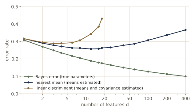
The Bayes error falls all the way. The nearest-mean classifier improves for a while and then deteriorates steadily: past some point, the noise in each new estimated mean difference outweighs the signal \(1/\sqrt{i}\). In fact its error tends to one half as \(d \to \infty\) with \(n\) fixed, although the Bayes error tends to zero. The linear discriminant estimates a whole covariance matrix, \(d(d+1)/2\) extra numbers, and it peaks much sooner and degrades much faster. The lesson is general: the number of samples needed grows with the number of parameters, and with too few samples a simpler model wins. DHS Figure 3.3 makes the complementary point, that projecting to fewer features can only increase the Bayes error; what the simulation shows is that with estimated parameters the Bayes error is not the quantity that matters.
Computational complexity
The second question is cost. We describe it with order notation. We write \(f(x) = O(h(x))\) (“big oh”) if there are constants \(c\) and \(x_0\) with \(\lvert f(x) \rvert \le c\lvert h(x) \rvert\) for all \(x > x_0\): for large \(x\), \(f\) grows no faster than \(h\). Big oh is only an upper bound, so \(f(x) = 3 + 2x + x^2\) is \(O(x^2)\) and also \(O(x^3)\). When we want the growth rate exactly we write \(f(x) = \Theta(h(x))\) (“big theta”), meaning \(c_1 h(x) \le f(x) \le c_2 h(x)\) for large \(x\); the quadratic above is \(\Theta(x^2)\) but not \(\Theta(x^3)\). DHS Appendix A.8 has the details.
Count the work to train a Gaussian classifier by maximum likelihood, with \(n\) samples per class in \(d\) dimensions and \(c\) classes. The discriminant for class \(\omega_i\) is
\[g_i(\mathbf{x}) = -\frac{1}{2}(\mathbf{x} - \hat{\boldsymbol{\mu}}_i)^t\hat{\boldsymbol{\Sigma}}_i^{-1}(\mathbf{x} - \hat{\boldsymbol{\mu}}_i) - \frac{d}{2}\ln 2\pi - \frac{1}{2}\ln\lvert\hat{\boldsymbol{\Sigma}}_i\rvert + \ln \hat P(\omega_i).\]| Step (per class) | Cost |
|---|---|
| sample mean: \(d\) sums of \(n\) numbers | \(O(nd)\) |
| sample covariance: \(d(d+1)/2\) entries, each a sum of \(n\) products | \(O(nd^2)\) |
| factor \(\hat{\boldsymbol{\Sigma}}\) (Cholesky), giving determinant and solves | \(O(d^3)\) |
| prior estimate | \(O(n)\) |
| training, all classes (\(n > d\)) | \(O(cnd^2)\) |
| classifying one \(\mathbf{x}\): a quadratic form per class, then a max | \(O(cd^2)\) |
With \(n > d\) the covariance term dominates, and since \(c\) is usually small, training is \(O(nd^2)\). Classification is much cheaper than training, as it is for almost every method in this course. The Bayesian Gaussian classifier with known covariance costs the same; general Bayesian learning, with its integrals over \(\boldsymbol{\theta}\), costs more. Constants matter for a particular problem size, but order notation is the standard way to compare algorithms. Sometimes we care about time complexity (sequential steps) and space complexity (memory, or processors) separately: \(d\) processors could compute the \(d\) components of a mean in parallel in \(O(n)\) time. And we distinguish polynomial algorithms from exponential ones, with cost like \(a^k\); the latter are hopeless beyond small sizes, and we meet one (and its polynomial replacement) with hidden Markov models at the end of this module.
The covariance count has a second consequence. \(\hat{\boldsymbol{\Sigma}}\) is a sum of \(n\) rank-one matrices whose centered vectors satisfy one linear constraint (they sum to zero), so its rank is at most \(n - 1\). It is singular whenever \(n \le d\): we need at least \(d + 1\) samples just to invert it, and several times that to estimate it well.
rng_r = np.random.default_rng(1)
d_r = 8
for n in [3, 5, 8, 9, 20]:
    _, S_hat = fit_gaussian_ml(rng_r.normal(size=(n, d_r)))
    rank = np.linalg.matrix_rank(S_hat)
    print(f"n = {n:2d} samples in d = {d_r}: rank of Sigma_hat = {rank}")
n =  3 samples in d = 8: rank of Sigma_hat = 2
n =  5 samples in d = 8: rank of Sigma_hat = 4
n =  8 samples in d = 8: rank of Sigma_hat = 7
n =  9 samples in d = 8: rank of Sigma_hat = 8
n = 20 samples in d = 8: rank of Sigma_hat = 8
The rank is \(n - 1\) until it reaches \(d\); with 8 or fewer samples in 8 dimensions the ML covariance cannot be inverted.
Overfitting
When the samples are too few for the model, there are several ways out. We can reduce the dimension: redesign the features, select a subset, or combine them (the component analysis of the next section, and module 10). We can assume all classes share one covariance and pool the data to estimate it. We can assume the features are independent, keeping only the diagonal of the covariance, which is almost surely false and yet often classifies better than the full ML estimate. Or we can look for a better estimate of \(\boldsymbol{\Sigma}\).
Why should a model we know to be wrong beat the right one? The same thing happens in curve fitting. Ten noisy points from a parabola are fit exactly by a polynomial of degree nine, which predicts new points badly, while a line or a parabola, fit with error on the training points, predicts better. Reliable interpolation needs an overdetermined fit: more data points than parameters. A full covariance per class is the high-degree polynomial of Gaussian classifiers. (Regression’s version of this story, with regularization and the bias–variance decomposition, is in Intro to ML, module 03; the classifier version returns in module 09.)
Shrinkage, also called regularized discriminant analysis, interpolates between these choices instead of picking one. With \(n_i\) samples in class \(i\), \(n = \sum_i n_i\), class ML covariances \(\hat{\boldsymbol{\Sigma}}_i\) and pooled covariance \(\hat{\boldsymbol{\Sigma}}\), each class covariance shrinks toward the pooled one,
\[\boldsymbol{\Sigma}_i(\alpha) = \frac{(1 - \alpha)\,n_i\hat{\boldsymbol{\Sigma}}_i + \alpha\,n\hat{\boldsymbol{\Sigma}}}{(1 - \alpha)\,n_i + \alpha\,n}, \qquad 0 < \alpha < 1,\]and the result can be shrunk further toward the identity,
\[\boldsymbol{\Sigma}(\beta) = (1 - \beta)\,\boldsymbol{\Sigma} + \beta\,\mathbf{I}, \qquad 0 < \beta < 1 .\]The second step damps the accidental correlations a small sample always shows, and makes the matrix invertible. Shrinking toward \(\mathbf{I}\) assumes the features are on comparable scales, so standardize them first. The same idea in regression is ridge regression.
The experiment: two classes in \(d = 8\) dimensions with different, correlated covariances and a mean difference that alternates in sign across features (so the correlations matter), 15 training samples per class, and a large test set. We train on 30 training sets and average the test error for a grid of \((\alpha, \beta)\).
def gaussian_scores(X, mus, Sigmas, priors=None):
    """Quadratic discriminants g_i(x) (without the common constant), one column per class."""
    cols = []
    for i, (mu, S) in enumerate(zip(mus, Sigmas)):
        L, low = cho_factor(S, lower=True)
        D = X - mu
        g = -0.5 * np.sum(D * cho_solve((L, low), D.T).T, axis=1) - np.sum(np.log(np.diag(L)))
        cols.append(g + (np.log(priors[i]) if priors is not None else 0.0))
    return np.column_stack(cols)

def shrink_cov(S_i, S_pool, n_i, n, alpha, beta):
    S_a = ((1 - alpha) * n_i * S_i + alpha * n * S_pool) / ((1 - alpha) * n_i + alpha * n)
    return (1 - beta) * S_a + beta * np.eye(len(S_i))

d_s = 8
idx = np.arange(d_s)
S1_true = 0.6 ** np.abs(idx[:, None] - idx[None, :])
D2 = np.diag(np.linspace(0.8, 1.25, d_s))
S2_true = D2 @ (0.4 ** np.abs(idx[:, None] - idx[None, :])) @ D2
mu1_true, mu2_true = np.zeros(d_s), 0.3 * (-1.0) ** idx

rng_sh = np.random.default_rng(55)
X_test = np.vstack([rng_sh.multivariate_normal(mu1_true, S1_true, 2000),
                    rng_sh.multivariate_normal(mu2_true, S2_true, 2000)])
y_test = np.repeat([0, 1], 2000)
g_true = gaussian_scores(X_test, [mu1_true, mu2_true], [S1_true, S2_true])
err_bayes = np.mean(g_true.argmax(1) != y_test)

alphas, betas = [0.0, 0.25, 0.5, 0.75, 1.0], [0.0, 0.05, 0.1, 0.2, 0.4, 1.0]
E = np.zeros((len(alphas), len(betas)))
n_per = 15
for rep in range(30):
    X1 = rng_sh.multivariate_normal(mu1_true, S1_true, n_per)
    X2 = rng_sh.multivariate_normal(mu2_true, S2_true, n_per)
    (m1, S1), (m2, S2) = fit_gaussian_ml(X1), fit_gaussian_ml(X2)
    S_pool = (S1 + S2) / 2
    for a, al in enumerate(alphas):
        for b, be in enumerate(betas):
            Ss = [shrink_cov(S, S_pool, n_per, 2 * n_per, al, be) for S in (S1, S2)]
            E[a, b] += np.mean(gaussian_scores(X_test, [m1, m2], Ss).argmax(1) != y_test) / 30
print(f"Bayes error (true parameters): {err_bayes:.3f}")
print("test error; rows alpha =", alphas, "; columns beta =", betas)
print(E)
Bayes error (true parameters): 0.202
test error; rows alpha = [0.0, 0.25, 0.5, 0.75, 1.0] ; columns beta = [0.0, 0.05, 0.1, 0.2, 0.4, 1.0]
[[0.3697 0.3528 0.3458 0.3402 0.343  0.3889]
 [0.3246 0.3212 0.3204 0.3233 0.3342 0.3889]
 [0.3128 0.3133 0.3148 0.3196 0.3335 0.3889]
 [0.312  0.3136 0.3157 0.3217 0.3364 0.3889]
 [0.316  0.3175 0.3202 0.326  0.3398 0.3889]]
The top-left entry (\(\alpha = \beta = 0\)) is the plain ML quadratic classifier, and it is the worst but one. The last column (\(\beta = 1\)) replaces both covariances by the identity and throws away the correlations the class separation depends on. Pooling (\(\alpha = 1\)) helps a great deal even though the true covariances differ, because it halves the number of covariance parameters, and partial pooling (\(\alpha\) between 0.5 and 0.75) does best of all. Shrinking toward the identity helps a lot when there is no pooling (along the first row the error drops from 0.370 to 0.340) but adds little once the pooled covariance is mixed in.
In practice. We picked the best cell by looking at test error, which a real design cannot do. Choose \(\alpha\) and \(\beta\) by cross-validation on the training set (module 09), standardize the features before shrinking toward \(\mathbf{I}\), and remember that the best amount of shrinkage falls as the number of samples per parameter grows.
Component analysis and discriminants
A direct response to too many features is to combine them into fewer. Linear combinations are the natural first choice: they are cheap and easy to analyze. A linear map projects the \(d\)-dimensional data onto a lower-dimensional subspace, and the question is which subspace. Principal component analysis (PCA) picks the subspace that represents the data best in the least-squares sense. Discriminant analysis picks the subspace that separates the classes best. They can give very different answers.
Principal component analysis
Start with the crudest representation: a single vector \(\mathbf{x}_0\) standing in for all \(n\) samples, chosen to minimize the squared-error criterion \(J_0(\mathbf{x}_0) = \sum_k \lVert \mathbf{x}_0 - \mathbf{x}_k \rVert^2\). With \(\mathbf{m}\) the sample mean, write \(\mathbf{x}_0 - \mathbf{x}_k = (\mathbf{x}_0 - \mathbf{m}) - (\mathbf{x}_k - \mathbf{m})\) and expand; the cross term is \(-2(\mathbf{x}_0 - \mathbf{m})^t\sum_k(\mathbf{x}_k - \mathbf{m}) = 0\), so
\[J_0(\mathbf{x}_0) = n\lVert \mathbf{x}_0 - \mathbf{m} \rVert^2 + \sum_{k=1}^{n}\lVert \mathbf{x}_k - \mathbf{m} \rVert^2 ,\]minimized by \(\mathbf{x}_0 = \mathbf{m}\). The mean is the best zero-dimensional summary, but it shows none of the spread.
Next, represent each sample by a point on a line through the mean, \(\mathbf{x}_k \approx \mathbf{m} + a_k\mathbf{e}\), with \(\lVert \mathbf{e} \rVert = 1\). For a fixed direction, minimizing \(\sum_k \lVert a_k\mathbf{e} - (\mathbf{x}_k - \mathbf{m}) \rVert^2\) over each \(a_k\) gives \(a_k = \mathbf{e}^t(\mathbf{x}_k - \mathbf{m})\), the orthogonal projection. Substituting back,
\[J_1(\mathbf{e}) = -\sum_{k=1}^{n}\left[\mathbf{e}^t(\mathbf{x}_k - \mathbf{m})\right]^2 + \sum_{k=1}^{n}\lVert \mathbf{x}_k - \mathbf{m} \rVert^2 = -\mathbf{e}^t\mathbf{S}\mathbf{e} + \sum_{k=1}^{n}\lVert \mathbf{x}_k - \mathbf{m} \rVert^2 ,\]where
\[\mathbf{S} = \sum_{k=1}^{n}(\mathbf{x}_k - \mathbf{m})(\mathbf{x}_k - \mathbf{m})^t\]is the scatter matrix, \(n - 1\) times the sample covariance. Minimizing \(J_1\) means maximizing \(\mathbf{e}^t\mathbf{S}\mathbf{e}\) subject to \(\mathbf{e}^t\mathbf{e} = 1\). With a Lagrange multiplier \(\lambda\), the gradient of \(\mathbf{e}^t\mathbf{S}\mathbf{e} - \lambda(\mathbf{e}^t\mathbf{e} - 1)\) is \(2\mathbf{S}\mathbf{e} - 2\lambda\mathbf{e}\), and setting it to zero gives
\[\mathbf{S}\mathbf{e} = \lambda\mathbf{e}.\]So \(\mathbf{e}\) is an eigenvector of the scatter matrix, and since \(\mathbf{e}^t\mathbf{S}\mathbf{e} = \lambda\), the best one belongs to the largest eigenvalue. The same argument extended to \(d' < d\) directions, \(\mathbf{x}_k \approx \mathbf{m} + \sum_{i=1}^{d'}a_{ki}\mathbf{e}_i\), shows that the best \(\mathbf{e}_1, \dots, \mathbf{e}_{d'}\) are the eigenvectors with the \(d'\) largest eigenvalues. Because \(\mathbf{S}\) is symmetric, these are orthogonal, the coefficients \(a_{ki}\) are the principal components of \(\mathbf{x}_k\), and the minimum squared error is the sum of the discarded eigenvalues. Geometrically, the eigenvectors are the axes of the ellipsoidal data cloud, and PCA keeps the directions along which the cloud is widest. Intro to ML, module 12 derives PCA a second way, as the directions of maximum variance, and gives it a probabilistic model.
def pca(X, k):
    """Mean, eigenvalues of the scatter matrix (descending), and the top-k eigenvectors."""
    m = X.mean(axis=0)
    S = (X - m).T @ (X - m)                       # scatter matrix
    lam, E = eigh(S)                              # ascending order
    order = np.argsort(lam)[::-1]
    return m, lam[order], E[:, order[:k]]

def pca_residual(X, m, E_k):
    """J = sum_k || x_k - (m + E_k a_k) ||^2 with a_k = E_k^t (x_k - m)."""
    D = X - m
    return np.sum((D - D @ E_k @ E_k.T) ** 2)

X5 = rng.multivariate_normal(np.zeros(5), np.diag([5.0, 3.0, 1.0, 0.5, 0.1]) + 0.3, size=300)
m5, lam5, _ = pca(X5, 5)
for k in range(6):
    _, _, E_k = pca(X5, k)
    print(f"k = {k}: residual {pca_residual(X5, m5, E_k):9.3f}"
          f"   sum of discarded eigenvalues {lam5[k:].sum():9.3f}")
k = 0: residual  3508.612   sum of discarded eigenvalues  3508.612
k = 1: residual  1751.086   sum of discarded eigenvalues  1751.086
k = 2: residual   714.781   sum of discarded eigenvalues   714.781
k = 3: residual   264.023   sum of discarded eigenvalues   264.023
k = 4: residual    57.273   sum of discarded eigenvalues    57.273
k = 5: residual     0.000   sum of discarded eigenvalues     0.000
The squared reconstruction error equals the sum of the eigenvalues we leave out, for every \(k\).
Fisher linear discriminant
PCA ignores the labels. The directions it discards as low-variance can be exactly the ones that tell the classes apart; think of the letters O and Q, which differ only in a small tail that barely affects the overall variance. Discriminant analysis looks for directions that are efficient for discrimination.
Take two classes, \(n_1\) samples in \(\mathcal{D}_1\) and \(n_2\) in \(\mathcal{D}_2\), and project each sample onto a line: \(y = \mathbf{w}^t\mathbf{x}\). The length of \(\mathbf{w}\) only rescales \(y\); its direction is what matters. The class means \(\mathbf{m}_i = \frac{1}{n_i}\sum_{\mathbf{x} \in \mathcal{D}_i}\mathbf{x}\) project to \(\tilde{m}_i = \mathbf{w}^t\mathbf{m}_i\). The distance between the projected means can be made as large as we like by scaling \(\mathbf{w}\), so it has to be measured against the spread of each projected class. Define the scatter of the projected class \(i\) as \(\tilde{s}_i^2 = \sum_{\mathbf{x} \in \mathcal{D}_i}(\mathbf{w}^t\mathbf{x} - \tilde{m}_i)^2\). The Fisher linear discriminant is the direction that maximizes
\[J(\mathbf{w}) = \frac{(\tilde{m}_1 - \tilde{m}_2)^2}{\tilde{s}_1^2 + \tilde{s}_2^2}.\]To write \(J\) in terms of \(\mathbf{w}\), define the class scatter matrices \(\mathbf{S}_i = \sum_{\mathbf{x} \in \mathcal{D}_i}(\mathbf{x} - \mathbf{m}_i)(\mathbf{x} - \mathbf{m}_i)^t\), the within-class scatter matrix \(\mathbf{S}_W = \mathbf{S}_1 + \mathbf{S}_2\), and the between-class scatter matrix \(\mathbf{S}_B = (\mathbf{m}_1 - \mathbf{m}_2)(\mathbf{m}_1 - \mathbf{m}_2)^t\). Then \(\tilde{s}_i^2 = \mathbf{w}^t\mathbf{S}_i\mathbf{w}\) and \((\tilde{m}_1 - \tilde{m}_2)^2 = \mathbf{w}^t\mathbf{S}_B\mathbf{w}\), so
\[J(\mathbf{w}) = \frac{\mathbf{w}^t\mathbf{S}_B\mathbf{w}}{\mathbf{w}^t\mathbf{S}_W\mathbf{w}},\]a generalized Rayleigh quotient. At a maximum the gradient vanishes, which (after multiplying through by the denominator) gives the generalized eigenvalue problem \(\mathbf{S}_B\mathbf{w} = \lambda\mathbf{S}_W\mathbf{w}\) with \(\lambda = J(\mathbf{w})\). Here we do not need an eigenvalue solver: \(\mathbf{S}_B\mathbf{w} = (\mathbf{m}_1 - \mathbf{m}_2)\left[(\mathbf{m}_1 - \mathbf{m}_2)^t\mathbf{w}\right]\) always points along \(\mathbf{m}_1 - \mathbf{m}_2\), so \(\mathbf{S}_W\mathbf{w} \propto \mathbf{m}_1 - \mathbf{m}_2\), and since the scale of \(\mathbf{w}\) is immaterial,
\[\mathbf{w} = \mathbf{S}_W^{-1}(\mathbf{m}_1 - \mathbf{m}_2).\]\(\mathbf{S}_W\) is symmetric and positive semidefinite, and nonsingular in the usual case \(n > d\); \(\mathbf{S}_B\) has rank one. Computing \(\mathbf{w}\) costs \(O(nd^2)\) for the scatter matrix plus a linear solve.
Fisher’s criterion gives a direction, not yet a classifier: we still need a threshold on \(y\). If the classes are Gaussian with a common covariance, the Bayes rule of module 02 is \(\mathbf{w}^t\mathbf{x} + w_0 > 0\) with \(\mathbf{w} = \boldsymbol{\Sigma}^{-1}(\boldsymbol{\mu}_1 - \boldsymbol{\mu}_2)\), and plugging in estimates gives a vector along Fisher’s direction (since \(\mathbf{S}_W\) is a multiple of the pooled covariance estimate). So in that case thresholding Fisher’s projection is the Bayes rule with estimated parameters. More generally we can fit a one-dimensional density to each projected class and put the threshold where the posteriors are equal. The projection loses information in principle, but a one-dimensional problem is far easier to estimate well.
The code uses one data set for both methods: two elongated classes whose long axes are parallel, placed side by side across the short axis. It computes the PCA and Fisher directions, confirms each by a brute-force scan over angles, and compares the best single threshold on each projection.
def fisher_direction(X1, X2):
    """w = S_W^{-1} (m1 - m2), normalized to unit length."""
    m1, m2 = X1.mean(0), X2.mean(0)
    S_W = (X1 - m1).T @ (X1 - m1) + (X2 - m2).T @ (X2 - m2)
    w = np.linalg.solve(S_W, m1 - m2)
    return w / np.linalg.norm(w), S_W

def fisher_J(w, X1, X2):
    y1, y2 = X1 @ w, X2 @ w
    s2 = np.sum((y1 - y1.mean()) ** 2) + np.sum((y2 - y2.mean()) ** 2)   # s1~^2 + s2~^2
    return (y1.mean() - y2.mean()) ** 2 / s2

def best_threshold_error(y1, y2):
    """Training error of the best single threshold on projected values, either orientation."""
    y, lab = np.r_[y1, y2], np.r_[np.zeros(len(y1)), np.ones(len(y2))]
    lab = lab[np.argsort(y)]
    below1 = np.r_[0, np.cumsum(lab == 0)]            # class-1 counts at or below each cut
    below2 = np.r_[0, np.cumsum(lab == 1)]
    e = np.minimum(below1 + (len(y2) - below2), below2 + (len(y1) - below1))
    return e.min() / len(y)

rng_f = np.random.default_rng(21)
ang = np.deg2rad(30)
R_f = np.array([[np.cos(ang), -np.sin(ang)], [np.sin(ang), np.cos(ang)]])
C_f = R_f @ np.diag([6.0, 0.25]) @ R_f.T                  # long axis at 30 degrees
shift = R_f @ np.array([0.0, 0.9])                        # offset across the short axis
XF1 = rng_f.multivariate_normal(shift, C_f, 100)
XF2 = rng_f.multivariate_normal(-shift, C_f, 100)
XF = np.vstack([XF1, XF2])

_, lam_f, E_f = pca(XF, 1)
e_pca = E_f[:, 0]
w_fish, S_W_f = fisher_direction(XF1, XF2)

thetas = np.deg2rad(np.linspace(0, 180, 180_001))
U = np.column_stack([np.cos(thetas), np.sin(thetas)])
mF = XF.mean(0)
spread = np.sum(((XF - mF) @ U.T) ** 2, axis=0)            # e^t S e along each direction
J_all = np.array([fisher_J(u, XF1, XF2) for u in U[::100]])   # coarser scan for J
deg = lambda v: np.degrees(np.arctan2(v[1], v[0])) % 180
scan_pca = np.degrees(thetas[np.argmax(spread)])
scan_fisher = np.degrees(thetas[::100][np.argmax(J_all)])
print(f"PCA direction    {deg(e_pca):7.2f} deg;  scan maximizing e^t S e: {scan_pca:7.2f}")
print(f"Fisher direction {deg(w_fish):7.2f} deg;  scan maximizing J(w):    {scan_fisher:7.2f}")
print(f"J(w): PCA direction {fisher_J(e_pca, XF1, XF2):.4f}"
      f"   Fisher direction {fisher_J(w_fish, XF1, XF2):.4f}")
err_pca = best_threshold_error(XF1 @ e_pca, XF2 @ e_pca)
print(f"best threshold error: PCA projection {err_pca:.3f}"
      f"   Fisher projection {best_threshold_error(XF1 @ w_fish, XF2 @ w_fish):.3f}")
PCA direction      29.33 deg;  scan maximizing e^t S e:   29.34
Fisher direction  118.09 deg;  scan maximizing J(w):     118.10
J(w): PCA direction 0.0000   Fisher direction 0.0847
best threshold error: PCA projection 0.460   Fisher projection 0.015
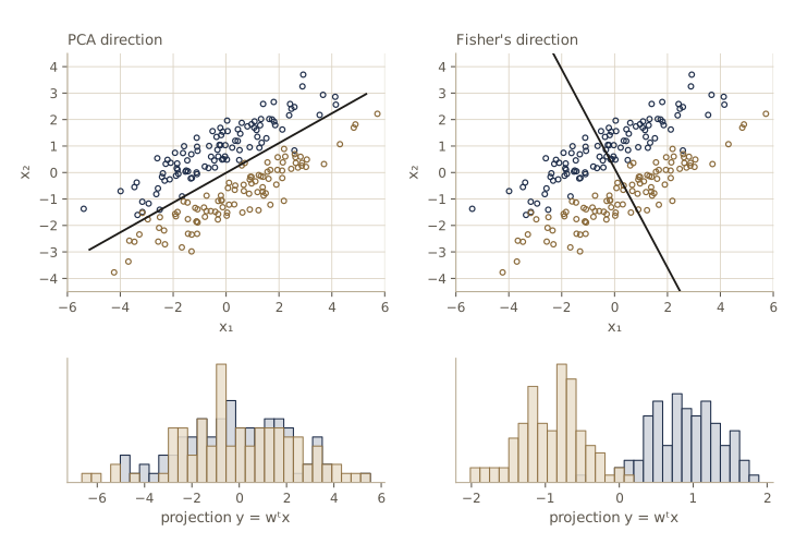
The scans agree with the closed forms. PCA chooses the long axis, where the classes lie on top of each other, and a threshold on that projection does little better than guessing. Fisher’s direction runs across the classes. It is not exactly perpendicular to the long axis: it tilts to account for the correlation within each class. For a longer treatment, including Fisher’s discriminant as a special case of least squares, see Intro to ML, module 04; the linear-machine view returns in module 05.
Multiple discriminant analysis
With \(c\) classes, Fisher’s idea generalizes to \(c - 1\) discriminant functions, a projection from \(d\) dimensions to \(c - 1\) (assuming \(d \ge c\)). The within-class scatter generalizes directly, \(\mathbf{S}_W = \sum_{i=1}^{c}\mathbf{S}_i\). For the between-class scatter, start from the total mean \(\mathbf{m} = \frac{1}{n}\sum_{\mathbf{x}}\mathbf{x} = \frac{1}{n}\sum_i n_i\mathbf{m}_i\) and the total scatter matrix \(\mathbf{S}_T = \sum_{\mathbf{x}}(\mathbf{x} - \mathbf{m})(\mathbf{x} - \mathbf{m})^t\). Writing \(\mathbf{x} - \mathbf{m} = (\mathbf{x} - \mathbf{m}_i) + (\mathbf{m}_i - \mathbf{m})\) for each \(\mathbf{x}\) in class \(i\) and expanding, the cross terms sum to zero within each class, leaving
\[\begin{gathered} \mathbf{S}_T = \mathbf{S}_W + \mathbf{S}_B, \\ \mathbf{S}_B = \sum_{i=1}^{c}n_i(\mathbf{m}_i - \mathbf{m})(\mathbf{m}_i - \mathbf{m})^t . \end{gathered}\]For two classes this \(\mathbf{S}_B\) is \(\frac{n_1n_2}{n}\) times the earlier one, which changes nothing about the optimal direction.
The projection is \(\mathbf{y} = \mathbf{W}^t\mathbf{x}\), with the \(c - 1\) weight vectors as the columns of the \(d \times (c-1)\) matrix \(\mathbf{W}\). The projected samples have scatter matrices \(\tilde{\mathbf{S}}_W = \mathbf{W}^t\mathbf{S}_W\mathbf{W}\) and \(\tilde{\mathbf{S}}_B = \mathbf{W}^t\mathbf{S}_B\mathbf{W}\). We need one number that measures the size of a scatter matrix; the determinant, the product of the variances along the principal axes (the squared volume of the scatter ellipsoid), is the classical choice. The criterion is
\[J(\mathbf{W}) = \frac{\lvert \tilde{\mathbf{S}}_B \rvert}{\lvert \tilde{\mathbf{S}}_W \rvert} = \frac{\lvert \mathbf{W}^t\mathbf{S}_B\mathbf{W} \rvert}{\lvert \mathbf{W}^t\mathbf{S}_W\mathbf{W} \rvert}.\]Maximizing over a rectangular matrix sounds hard, but the answer is simple: the columns of an optimal \(\mathbf{W}\) are the generalized eigenvectors of
\[\mathbf{S}_B\mathbf{w}_i = \lambda_i\mathbf{S}_W\mathbf{w}_i\]with the largest eigenvalues. A symmetric-definite generalized eigensolver (here scipy.linalg.eigh(S_B, S_W)) solves this without forming \(\mathbf{S}_W^{-1}\). Since \(\mathbf{S}_B\) is a sum of \(c\) rank-one matrices whose vectors \(n_i(\mathbf{m}_i - \mathbf{m})\) sum to zero, its rank is at most \(c - 1\), and at most \(c - 1\) eigenvalues are nonzero. The solution is not unique: any invertible \((c-1) \times (c-1)\) matrix \(\mathbf{A}\) gives \(\mathbf{W}\mathbf{A}\) with the same \(J\), because both determinants pick up the factor \(\lvert\mathbf{A}\rvert^2\). Rotations and rescalings of the projected axes do not change the classifier we build there.
The code checks each of these claims on three classes in five dimensions.
def mda(X, y, k):
    """MDA: the top-k generalized eigenvectors of S_B w = lambda S_W w."""
    m = X.mean(axis=0)
    d = X.shape[1]
    S_W, S_B = np.zeros((d, d)), np.zeros((d, d))
    for c in np.unique(y):
        Xc = X[y == c]
        mc = Xc.mean(axis=0)
        S_W += (Xc - mc).T @ (Xc - mc)
        S_B += len(Xc) * np.outer(mc - m, mc - m)
    lam, V = eigh(S_B, S_W)                     # generalized symmetric-definite problem
    order = np.argsort(lam)[::-1]
    return V[:, order[:k]], lam[order], S_W, S_B

def mda_J(W, S_W, S_B):
    return np.linalg.det(W.T @ S_B @ W) / np.linalg.det(W.T @ S_W @ W)

rng_m = np.random.default_rng(33)
means_m = np.array([[0, 0, 0, 0, 0], [2, 1, 0, 0, 0], [1, 3, 1, 0, 0]], dtype=float)
C_m = np.eye(5) + 0.5
X_m = np.vstack([rng_m.multivariate_normal(mu, C_m, 60) for mu in means_m])
y_m = np.repeat(np.arange(3), 60)

W_m, lam_m, S_W_m, S_B_m = mda(X_m, y_m, 2)
S_T_m = (X_m - X_m.mean(0)).T @ (X_m - X_m.mean(0))
print(f"max |S_T - (S_W + S_B)| = {np.abs(S_T_m - S_W_m - S_B_m).max():.1e}")
print("generalized eigenvalues:", lam_m)
J_opt = mda_J(W_m, S_W_m, S_B_m)
J_rand = max(mda_J(rng_m.normal(size=(5, 2)), S_W_m, S_B_m) for _ in range(5000))
A_m = rng_m.normal(size=(2, 2))
print(f"J at the MDA solution {J_opt:.4f};  best of 5000 random W {J_rand:.4f};"
      f"  J(W A) {mda_J(W_m @ A_m, S_W_m, S_B_m):.4f}")

W2, _, _, _ = mda(XF, np.repeat([0, 1], 100), 1)          # two classes: MDA = Fisher
cosine = abs(W2[:, 0] @ w_fish) / np.linalg.norm(W2[:, 0])
print(f"two classes: |cos(angle)| between MDA and Fisher directions = {cosine:.6f}")
max |S_T - (S_W + S_B)| = 3.1e-13
generalized eigenvalues: [ 1.3972  0.7379  0.      0.     -0.    ]
J at the MDA solution 1.0310;  best of 5000 random W 0.9233;  J(W A) 1.0310
two classes: |cos(angle)| between MDA and Fisher directions = 1.000000
Two of the five eigenvalues are nonzero, as the rank argument predicts, and the product of those two is exactly \(J\) at the solution. No random projection beats it, and multiplying \(\mathbf{W}\) by an arbitrary \(2 \times 2\) matrix leaves \(J\) unchanged. For two classes MDA returns Fisher’s direction.
MDA is primarily a way to reduce dimension. In the \((c-1)\)-dimensional projected space, methods that were impractical in \(d\) dimensions (a full covariance per class, or the nonparametric methods of module 04) may become feasible. With little data one projects to fewer dimensions still. If the projection mixes classes that were separable in the original space, no later classifier can undo the damage.
Expectation-maximization
Module 02 showed how to classify a test point with missing features. The expectation-maximization (EM) algorithm handles the harder problem of training when some features are missing. Write each sample as \(\mathbf{x}_k = \{\mathbf{x}_{kg}, \mathbf{x}_{kb}\}\), its “good” (observed) and “bad” (missing) features, and collect them into \(\mathcal{D}_g\) and \(\mathcal{D}_b\). We want the ML estimate based on what we actually have: maximize the observed-data log-likelihood
\[l(\boldsymbol{\theta}) = \ln p(\mathcal{D}_g; \boldsymbol{\theta}) = \ln\int p(\mathcal{D}_g, \mathcal{D}_b; \boldsymbol{\theta})\,d\mathcal{D}_b ,\]in which the missing values are integrated out. The integral inside the logarithm usually makes direct maximization awkward. EM replaces it with a sequence of easier problems. Given a current estimate \(\boldsymbol{\theta}^i\), define
\[Q(\boldsymbol{\theta}; \boldsymbol{\theta}^i) = \mathbb{E}_{\mathcal{D}_b}\left[\ln p(\mathcal{D}_g, \mathcal{D}_b; \boldsymbol{\theta}) \mid \mathcal{D}_g; \boldsymbol{\theta}^i\right],\]the complete-data log-likelihood at a candidate \(\boldsymbol{\theta}\), averaged over the missing values as distributed under the current estimate. (The semicolons mark which argument is being varied and which is held fixed.) The algorithm alternates two steps until the improvement is below a tolerance:
- E step: compute \(Q(\boldsymbol{\theta}; \boldsymbol{\theta}^i)\), which in practice means computing the expected values it needs.
- M step: set \(\boldsymbol{\theta}^{i+1} = \arg\max_{\boldsymbol{\theta}} Q(\boldsymbol{\theta}; \boldsymbol{\theta}^i)\).
EM pays off when maximizing \(Q\) is easy, which is common: often it is an ordinary complete-data ML problem with the missing quantities replaced by their expectations.
Why the likelihood never decreases. Since \(p(\mathcal{D}_g, \mathcal{D}_b; \boldsymbol{\theta}) = p(\mathcal{D}_b \mid \mathcal{D}_g; \boldsymbol{\theta})\,p(\mathcal{D}_g; \boldsymbol{\theta})\), taking logs and averaging over \(\mathcal{D}_b\) under \(\boldsymbol{\theta}^i\) gives
\[\begin{gathered} l(\boldsymbol{\theta}) = Q(\boldsymbol{\theta}; \boldsymbol{\theta}^i) + H(\boldsymbol{\theta}; \boldsymbol{\theta}^i), \\ H(\boldsymbol{\theta}; \boldsymbol{\theta}^i) = -\mathbb{E}_{\mathcal{D}_b}\left[\ln p(\mathcal{D}_b \mid \mathcal{D}_g; \boldsymbol{\theta}) \mid \mathcal{D}_g; \boldsymbol{\theta}^i\right]. \end{gathered}\]\(H\) is a cross-entropy between the conditional distribution of the missing data under \(\boldsymbol{\theta}^i\) and under \(\boldsymbol{\theta}\), and Gibbs’ inequality says it is smallest when the two agree: \(H(\boldsymbol{\theta}; \boldsymbol{\theta}^i) \ge H(\boldsymbol{\theta}^i; \boldsymbol{\theta}^i)\). Therefore
\[l(\boldsymbol{\theta}^{i+1}) - l(\boldsymbol{\theta}^i) \ge Q(\boldsymbol{\theta}^{i+1}; \boldsymbol{\theta}^i) - Q(\boldsymbol{\theta}^i; \boldsymbol{\theta}^i) \ge 0,\]the last step because \(\boldsymbol{\theta}^{i+1}\) maximizes \(Q\). Any update that merely increases \(Q\) keeps the guarantee; such methods are generalized EM (GEM) algorithms, and they trade slower convergence for cheaper M steps. EM converges to a stationary point of \(l\), possibly a local maximum, not necessarily the global one. The general theory, with mixture models as the main example, is in Intro to ML, module 09; unsupervised learning with EM for mixtures is the subject of module 10.
Watch out. EM maximizes the likelihood of the observed data with the missing values integrated out. That is not the same as choosing the most likely values for the missing entries and then fitting: filling in values treats guesses as if they were measurements. In the example below, filling in the conditional means and refitting underestimates the variances.
EM for a Gaussian with missing features
Let the complete data be \(N(\boldsymbol{\mu}, \boldsymbol{\Sigma})\) with a full covariance. The complete-data log-likelihood
\[\ln p(\mathcal{D}; \boldsymbol{\theta}) = -\frac{n}{2}\ln\lvert\boldsymbol{\Sigma}\rvert - \frac{1}{2}\operatorname{tr}\left(\boldsymbol{\Sigma}^{-1}\sum_{k=1}^{n}\left(\mathbf{x}_k\mathbf{x}_k^t - \mathbf{x}_k\boldsymbol{\mu}^t - \boldsymbol{\mu}\mathbf{x}_k^t + \boldsymbol{\mu}\boldsymbol{\mu}^t\right)\right) + \text{const}\]depends on the data only through \(\sum_k\mathbf{x}_k\) and \(\sum_k\mathbf{x}_k\mathbf{x}_k^t\), the Gaussian’s sufficient statistics, and it is linear in them. So the E step only has to compute their expected values, and the M step is ordinary Gaussian ML with the expectations in place of the raw sums:
\[\begin{gathered} \boldsymbol{\mu}^{i+1} = \frac{1}{n}\sum_{k=1}^{n}\hat{\mathbf{x}}_k, \\ \boldsymbol{\Sigma}^{i+1} = \frac{1}{n}\sum_{k=1}^{n}\mathbb{E}\left[\mathbf{x}_k\mathbf{x}_k^t\right] - \boldsymbol{\mu}^{i+1}(\boldsymbol{\mu}^{i+1})^t , \end{gathered}\]where \(\hat{\mathbf{x}}_k = \mathbb{E}[\mathbf{x}_k \mid \mathbf{x}_{kg}; \boldsymbol{\theta}^i]\). For the expectations, partition \(\boldsymbol{\mu}\) and \(\boldsymbol{\Sigma}\) into observed (\(g\)) and missing (\(b\)) blocks for sample \(k\). The conditional distribution of the missing block given the observed one is Gaussian, with
\[\begin{gathered} \mathbb{E}[\mathbf{x}_{kb} \mid \mathbf{x}_{kg}] = \boldsymbol{\mu}_b + \boldsymbol{\Sigma}_{bg}\boldsymbol{\Sigma}_{gg}^{-1}(\mathbf{x}_{kg} - \boldsymbol{\mu}_g), \\ \operatorname{Cov}[\mathbf{x}_{kb} \mid \mathbf{x}_{kg}] = \boldsymbol{\Sigma}_{bb} - \boldsymbol{\Sigma}_{bg}\boldsymbol{\Sigma}_{gg}^{-1}\boldsymbol{\Sigma}_{gb}. \end{gathered}\]So \(\hat{\mathbf{x}}_k\) keeps the observed values and fills the missing block with its conditional mean, and \(\mathbb{E}[\mathbf{x}_k\mathbf{x}_k^t] = \hat{\mathbf{x}}_k\hat{\mathbf{x}}_k^t + \mathbf{C}_k\), where \(\mathbf{C}_k\) is the conditional covariance placed in the missing-missing block and zero elsewhere. That \(\mathbf{C}_k\) term is exactly what single imputation forgets.
Our data: 80 points from a correlated two-dimensional Gaussian. For 25 of them the first coordinate is deleted, and for 15 others the second, chosen at random regardless of the values (so the missingness carries no information of its own). The observed-data log-likelihood is a sum over samples of Gaussian log-densities of the observed coordinates only, since marginals of a Gaussian are Gaussian.
def observed_loglik(X, mu, Sigma):
    """ln p(D_g; theta): each sample contributes the marginal density of its observed part."""
    total = 0.0
    for x in X:
        g = ~np.isnan(x)
        if g.any():
            total += stats.multivariate_normal(mu[g], Sigma[np.ix_(g, g)]).logpdf(x[g])
    return total

def em_gaussian_missing(X, n_iter=500, tol=1e-12):
    """EM for N(mu, Sigma) with missing entries (np.nan).
    Returns mu, Sigma, the log-likelihood history, and the filled-in data."""
    n, d = X.shape
    miss = np.isnan(X)
    mu = np.nanmean(X, axis=0)                          # start: observed means and variances,
    Sigma = np.diag(np.nanvar(X, axis=0))               # no correlation
    history = [observed_loglik(X, mu, Sigma)]
    for _ in range(n_iter):
        X_hat = np.where(miss, 0.0, X)                  # E step: expected x and x x^t
        sum_xx = np.zeros((d, d))
        for k in range(n):
            b, g = miss[k], ~miss[k]
            C_k = np.zeros((d, d))
            if b.any():
                if g.any():
                    # K = Sigma_bg Sigma_gg^{-1}
                    K = np.linalg.solve(Sigma[np.ix_(g, g)], Sigma[np.ix_(g, b)]).T
                    X_hat[k, b] = mu[b] + K @ (X[k, g] - mu[g])
                    C_k[np.ix_(b, b)] = Sigma[np.ix_(b, b)] - K @ Sigma[np.ix_(g, b)]
                else:
                    X_hat[k] = mu
                    C_k = Sigma.copy()
            sum_xx += np.outer(X_hat[k], X_hat[k]) + C_k
        mu = X_hat.mean(axis=0)                         # M step: ML with expected statistics
        Sigma = sum_xx / n - np.outer(mu, mu)
        history.append(observed_loglik(X, mu, Sigma))
        if history[-1] - history[-2] < tol:
            break
    return mu, Sigma, np.array(history), X_hat

rng_e = np.random.default_rng(77)
mu_e_true = np.array([1.0, 2.0])
Sigma_e_true = np.array([[1.0, 0.8], [0.8, 1.5]])
X_full = rng_e.multivariate_normal(mu_e_true, Sigma_e_true, size=80)
X_miss = X_full.copy()
perm = rng_e.permutation(80)
X_miss[perm[:25], 0] = np.nan                           # 25 points lose x1
X_miss[perm[25:40], 1] = np.nan                         # 15 others lose x2

mu_em, Sigma_em, ll_hist, X_filled = em_gaussian_missing(X_miss)
print(f"iterations: {len(ll_hist) - 1};  observed-data log-likelihood at checkpoints:")
for i in [0, 1, 2, 3, 5, 10, len(ll_hist) - 1]:
    print(f"   iteration {i:3d}: {ll_hist[i]:.6f}")
print(f"smallest change between iterations: {np.diff(ll_hist).min():.2e}  (never negative)")
iterations: 27;  observed-data log-likelihood at checkpoints:
   iteration   0: -186.784773
   iteration   1: -180.277520
   iteration   2: -177.391168
   iteration   3: -176.146860
   iteration   5: -175.513289
   iteration  10: -175.440089
   iteration  27: -175.439921
smallest change between iterations: 3.41e-13  (never negative)
Each iteration raises the observed-data log-likelihood, quickly at first and then by ever smaller amounts. At the end we check that EM stopped at a stationary point of \(l\) itself, by finite differences, and compare its estimates with three alternatives: the complete-case estimate (throw away every point with a missing value), single imputation (fill in the conditional means from the final EM fit and estimate as if nothing were missing), and the ML estimate from the full data before we deleted anything.
slope_em = max_slope(lambda m, S: observed_loglik(X_miss, m, S), mu_em, Sigma_em)
print(f"largest slope of l at the EM estimate: {slope_em:.1e}")
complete = ~np.isnan(X_miss).any(axis=1)
fits = {"EM": (mu_em, Sigma_em),
        "complete cases only": fit_gaussian_ml(X_miss[complete]),
        "single imputation": fit_gaussian_ml(X_filled),
        "full data (no deletion)": fit_gaussian_ml(X_full)}
print(f"{'':25s} mu1     mu2    var1    var2    cov12")
for name, (m_, S_) in fits.items():
    print(f"{name:25s} {m_[0]:.3f}  {m_[1]:.3f}"
          f"  {S_[0, 0]:.3f}  {S_[1, 1]:.3f}  {S_[0, 1]:.3f}")
largest slope of l at the EM estimate: 5.0e-06
                          mu1     mu2    var1    var2    cov12
EM                        1.163  2.087  1.129  1.547  0.897
complete cases only       1.113  2.017  1.112  1.330  0.802
single imputation         1.163  2.087  0.939  1.391  0.897
full data (no deletion)   1.083  2.079  1.053  1.498  0.864
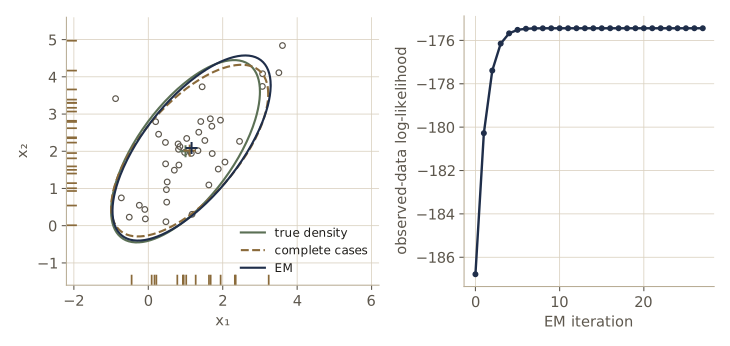
The slope of \(l\) at the EM estimate is zero to finite-difference accuracy, so EM found the observed-data ML estimate. The EM estimates use every observed number and land close to the full-data estimates. The complete-case fit discards half of the sample, and single imputation shrinks both variances because the filled-in points lie exactly on the regression line, with none of the scatter real points would have.
Hidden Markov models
So far each decision concerned a single pattern. Many problems produce sequences in which each element depends on what came before: the sounds of a spoken word, the strokes of a gesture, the symbols of a signal. Hidden Markov models (HMMs) model such sequences with a small set of unobserved states. The estimation ideas are the ones we already have (maximum likelihood, EM); what is new is the bookkeeping over time, and the dynamic-programming algorithms that make it affordable. For classification we train one HMM per class and assign a test sequence to the model under which it is most probable.
First-order Markov models
Let the system occupy one of \(c\) states at each time step. The state at time \(t\) is \(\omega(t)\), and a sequence of length \(T\) is \(\boldsymbol{\omega}^T = \{\omega(1), \omega(2), \dots, \omega(T)\}\); states may repeat, and not every state need appear. In a first-order Markov model the next state depends only on the current one, through the time-independent transition probabilities
\[a_{ij} = P(\omega_j(t+1) \mid \omega_i(t)),\]where \(\omega_i(t)\) means “the state at time \(t\) is \(\omega_i\)”. Transitions need not be symmetric (\(a_{ij} \neq a_{ji}\) in general), and a state may follow itself (\(a_{ii} > 0\)). We also need a distribution for the first state; we write \(\pi_i = P(\omega(1) = \omega_i)\). (DHS instead start the system in a known state at \(t = 0\), which is the special case where \(\boldsymbol{\pi}\) is one row of the transition matrix.) The probability of a state sequence is a product along the sequence:
\[P(\boldsymbol{\omega}^T) = \pi_{\omega(1)}\prod_{t=2}^{T}a_{\omega(t-1)\,\omega(t)} .\]First-order hidden Markov models
In most applications we cannot see the states. A speech recognizer hears sounds, not phonemes. So at each step the state emits a visible symbol \(v(t)\) from a finite alphabet \(\{v_1, \dots, v_M\}\), with emission probabilities
\[b_{jk} = P(v_k(t) \mid \omega_j(t)),\]the probability that state \(\omega_j\) emits symbol \(v_k\). We observe the visible sequence \(\mathbf{V}^T = \{v(1), \dots, v(T)\}\); the state sequence that produced it is hidden. That is a hidden Markov model. Richer HMMs emit continuous vectors (spectra, for example) from a density per state; we stay with discrete symbols.
Hidden Markov model computation
A few terms. A network of states with transitions is a finite-state machine, and with transition probabilities attached, a Markov network. A model is ergodic if every state can be reached, with nonzero probability, from any starting state. A final or absorbing state \(\omega_0\) is one that is never left, \(a_{00} = 1\); DHS use one to mark the end of a sequence (with a special “silence” symbol \(v_0\)). A left-to-right model only allows transitions to the same or a later state, and is the usual structure in speech recognition, where a word is a fixed order of sounds.
Some transition must happen at every step (possibly back to the same state) and some symbol must be emitted, so the rows of both matrices sum to one:
\[\sum_{j} a_{ij} = 1 \;\text{ for all } i, \qquad \sum_{k} b_{jk} = 1 \;\text{ for all } j .\]The three central problems are:
- Evaluation. Given the model \(\boldsymbol{\theta} = (\boldsymbol{\pi}, \mathbf{A}, \mathbf{B})\), compute the probability \(P(\mathbf{V}^T \mid \boldsymbol{\theta})\) of a visible sequence. This is what classification needs.
- Decoding. Given the model and \(\mathbf{V}^T\), find the most probable hidden state sequence.
- Learning. Given the number of states and symbols and a set of training sequences, estimate \(\boldsymbol{\pi}\), \(a_{ij}\), and \(b_{jk}\).
Our running model has \(c = 3\) states and \(M = 4\) symbols, and cycles \(\omega_1 \to \omega_2 \to \omega_3 \to \omega_1\) with self-loops; the other transitions are forbidden (probability zero). In code, states and symbols are indexed from 0. The helper sample_hmm generates sequences from a model.
pi_h = np.array([0.5, 0.3, 0.2])
A_h = np.array([[0.6, 0.4, 0.0],        # a_ij = P(state j at t+1 | state i at t)
                [0.0, 0.5, 0.5],
                [0.3, 0.0, 0.7]])
B_h = np.array([[0.6, 0.3, 0.1, 0.0],   # b_jk = P(symbol k | state j)
                [0.1, 0.3, 0.5, 0.1],
                [0.1, 0.2, 0.2, 0.5]])

def sample_hmm(pi, A, B, T, rng_s):
    states, symbols = np.zeros(T, int), np.zeros(T, int)
    s = rng_s.choice(len(pi), p=pi)
    for t in range(T):
        states[t], symbols[t] = s, rng_s.choice(B.shape[1], p=B[s])
        s = rng_s.choice(len(pi), p=A[s])
    return states, symbols

print("row sums of A:", A_h.sum(1), "  row sums of B:", B_h.sum(1))
print("one sampled sequence (states, symbols):")
st, sy = sample_hmm(pi_h, A_h, B_h, 12, np.random.default_rng(4))
print(st, "\n", sy)
row sums of A: [1. 1. 1.]   row sums of B: [1. 1. 1.]
one sampled sequence (states, symbols):
[2 2 2 2 2 2 2 2 2 0 1 2]
 [3 0 2 1 3 2 3 2 3 1 3 1]
Evaluation
The direct approach sums over every hidden path. For each of the \(c^T\) state sequences \(\boldsymbol{\omega}_r^T\), the probability of the path is the product of transitions and the probability of the visible sequence along it is the product of emissions:
\[\begin{aligned} P(\mathbf{V}^T) &= \sum_{r=1}^{c^T} P(\mathbf{V}^T \mid \boldsymbol{\omega}_r^T)\,P(\boldsymbol{\omega}_r^T) \\ &= \sum_{r=1}^{c^T} \pi_{\omega(1)}b_{\omega(1)v(1)}\prod_{t=2}^{T}a_{\omega(t-1)\omega(t)}\,b_{\omega(t)v(t)} . \end{aligned}\]That is \(O(c^T T)\) work, exponential in the length. With 10 states and 20 time steps it is on the order of \(10^{21}\) operations.
The paths share almost all of their structure, and the forward algorithm exploits it. Define \(\alpha_j(t)\) as the probability of emitting the first \(t\) symbols and being in state \(\omega_j\) at time \(t\). Every path into \(\omega_j\) at time \(t\) comes from some state \(\omega_i\) at time \(t - 1\), so
\[\begin{gathered} \alpha_j(1) = \pi_j\,b_{jv(1)}, \\ \alpha_j(t) = b_{jv(t)}\sum_{i=1}^{c}\alpha_i(t-1)\,a_{ij}, \\ P(\mathbf{V}^T) = \sum_{j=1}^{c}\alpha_j(T), \end{gathered}\]where \(b_{jv(t)}\) is the emission probability of the symbol actually observed at time \(t\). Each step costs \(O(c^2)\), so the whole computation is \(O(c^2T)\): about 2000 operations instead of \(10^{21}\) in the example above. The computation is easiest to picture on a trellis, the HMM unrolled in time, with one column of states per time step.
The backward algorithm runs the same idea from the other end. Define \(\beta_i(t)\) as the probability of emitting the rest of the sequence, \(v(t+1), \dots, v(T)\), given state \(\omega_i\) at time \(t\):
\[\begin{gathered} \beta_i(T) = 1, \\ \beta_i(t) = \sum_{j=1}^{c}a_{ij}\,b_{jv(t+1)}\,\beta_j(t+1), \\ P(\mathbf{V}^T) = \sum_{i=1}^{c}\pi_i\,b_{iv(1)}\,\beta_i(1). \end{gathered}\]Since \(\alpha_i(t)\beta_i(t)\) is the probability of the whole sequence together with state \(\omega_i\) at time \(t\), summing over \(i\) gives \(P(\mathbf{V}^T)\) at every \(t\), a useful check. With DHS’s absorbing final state, \(P(\mathbf{V}^T)\) is \(\alpha_0(T)\) for that state instead of the sum over all \(j\), and \(\beta\) is initialized to 1 only at \(\omega_0\).
Probabilities of long sequences underflow, so we work with logarithms, replacing sums of products by logsumexp of sums. The code checks the forward and backward results against brute-force enumeration of all \(3^7 = 2187\) paths for a sequence of length 7, and checks the identity at every \(t\).
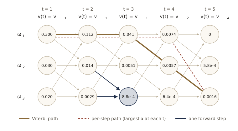
def forward_log(V, pi, A, B):
    """log alpha_j(t) for a symbol sequence V (log space: long sequences do not underflow)."""
    with np.errstate(divide="ignore"):
        lA, lB, lpi = np.log(A), np.log(B), np.log(pi)
    la = np.zeros((len(V), len(pi)))
    la[0] = lpi + lB[:, V[0]]
    for t in range(1, len(V)):
        # alpha_j(t) = b_j,v(t) * sum_i alpha_i(t-1) a_ij
        la[t] = lB[:, V[t]] + logsumexp(la[t - 1][:, None] + lA, axis=0)
    return la

def backward_log(V, pi, A, B):
    """log beta_i(t)."""
    with np.errstate(divide="ignore"):
        lA, lB = np.log(A), np.log(B)
    lb = np.zeros((len(V), len(pi)))                   # beta_i(T) = 1
    for t in range(len(V) - 2, -1, -1):
        lb[t] = logsumexp(lA + lB[:, V[t + 1]] + lb[t + 1], axis=1)       # sum over j
    return lb

def path_prob(path, V, pi, A, B):
    p = pi[path[0]] * B[path[0], V[0]]
    for t in range(1, len(V)):
        p *= A[path[t - 1], path[t]] * B[path[t], V[t]]
    return p

V7 = np.array([0, 1, 2, 2, 3, 0, 1])
all_paths = list(product(range(3), repeat=len(V7)))
p_brute = sum(path_prob(p, V7, pi_h, A_h, B_h) for p in all_paths)
la7, lb7 = forward_log(V7, pi_h, A_h, B_h), backward_log(V7, pi_h, A_h, B_h)
with np.errstate(divide="ignore"):
    p_back = np.exp(logsumexp(np.log(pi_h) + np.log(B_h[:, V7[0]]) + lb7[0]))
print(f"brute force over {len(all_paths)} paths: P(V) = {p_brute:.10e}")
print(f"forward:  {np.exp(logsumexp(la7[-1])):.10e}")
print(f"backward: {p_back:.10e}")
ab = np.exp(logsumexp(la7 + lb7, axis=1))           # one value per t = 1..7
print(f"sum_i alpha_i(t) beta_i(t) over t = 1..7: min {ab.min():.10e}, max {ab.max():.10e}")
brute force over 2187 paths: P(V) = 1.8209642035e-04
forward:  1.8209642035e-04
backward: 1.8209642035e-04
sum_i alpha_i(t) beta_i(t) over t = 1..7: min 1.8209642035e-04, max 1.8209642035e-04
For classification with several HMMs, one per class, Bayes’ formula gives the posterior of each model,
\[P(\boldsymbol{\theta} \mid \mathbf{V}^T) = \frac{P(\mathbf{V}^T \mid \boldsymbol{\theta})\,P(\boldsymbol{\theta})}{P(\mathbf{V}^T)},\]and we choose the model with the largest posterior. The forward algorithm supplies \(P(\mathbf{V}^T \mid \boldsymbol{\theta})\). The prior \(P(\boldsymbol{\theta})\) comes from outside, for instance from a language model that says which words are likely in context; without such knowledge it is taken to be equal for all models, another use of a noninformative prior.
Decoding
Decoding asks for the single most probable hidden path,
\[\hat{\boldsymbol{\omega}}^T = \arg\max_{\boldsymbol{\omega}^T} P(\boldsymbol{\omega}^T, \mathbf{V}^T),\]again a search over \(c^T\) paths if done naively. The Viterbi algorithm replaces the sum in the forward recursion by a maximum and remembers where each maximum came from. Let \(\delta_j(t)\) be the probability of the best partial path that emits the first \(t\) symbols and ends in \(\omega_j\):
\[\begin{gathered} \delta_j(1) = \pi_j\,b_{jv(1)}, \\ \delta_j(t) = b_{jv(t)}\max_{i}\,\delta_i(t-1)\,a_{ij}, \\ \psi_j(t) = \arg\max_{i}\,\delta_i(t-1)\,a_{ij}. \end{gathered}\]The best final state is \(\arg\max_j \delta_j(T)\), and following the back-pointers \(\psi\) from there recovers the whole path. This works because the best path through \(\omega_j\) at time \(t\) must begin with the best path into \(\omega_j\) at time \(t\) (dynamic programming). The cost is \(O(c^2T)\), and in log space the products become sums.
Watch out. The decoding algorithm printed in DHS §3.10.5 (Algorithm 4 in our copy of the book) is not Viterbi. It runs the forward recursion and, at each step, appends the state with the largest \(\alpha_j(t)\). Those states are chosen one time step at a time, so the resulting “path” can contain a transition the model forbids, as the book itself warns. The Viterbi algorithm maximizes over whole paths and always returns a valid one. The code below compares the two.
The code implements Viterbi in log space, checks it against brute force on the length-7 sequence, and then examines the per-step rule on every sequence of length 5.
def viterbi_log(V, pi, A, B):
    """Most probable state path and its log probability (log-space Viterbi)."""
    with np.errstate(divide="ignore"):
        lA, lB, lpi = np.log(A), np.log(B), np.log(pi)
    T, c = len(V), len(pi)
    ld = np.zeros((T, c))
    psi = np.zeros((T, c), dtype=int)
    ld[0] = lpi + lB[:, V[0]]
    for t in range(1, T):
        scores = ld[t - 1][:, None] + lA        # [i, j] = log delta_i(t-1) + log a_ij
        psi[t] = np.argmax(scores, axis=0)
        ld[t] = lB[:, V[t]] + scores[psi[t], np.arange(c)]
    path = np.zeros(T, dtype=int)
    path[-1] = np.argmax(ld[-1])
    for t in range(T - 1, 0, -1):                         # follow the back-pointers
        path[t - 1] = psi[t, path[t]]
    return path, ld[-1].max()

path_v, lp_v = viterbi_log(V7, pi_h, A_h, B_h)
best_brute = max(all_paths, key=lambda p: path_prob(p, V7, pi_h, A_h, B_h))
print("Viterbi path:", path_v, f" log P = {lp_v:.6f}")
lp_brute = np.log(path_prob(best_brute, V7, pi_h, A_h, B_h))
print("brute force: ", np.array(best_brute), f" log P = {lp_brute:.6f}")

def per_step_path(V, pi, A, B):
    """The per-step rule: at each t take the state with the largest alpha_j(t)."""
    return np.argmax(forward_log(V, pi, A, B), axis=1)

n_seq = n_invalid = n_differ = 0
mass_invalid = 0.0
example = None
for V in product(range(4), repeat=5):
    V = np.array(V)
    la = forward_log(V, pi_h, A_h, B_h)
    pV = np.exp(logsumexp(la[-1]))
    if pV == 0:
        continue
    n_seq += 1
    greedy = per_step_path(V, pi_h, A_h, B_h)
    vit, _ = viterbi_log(V, pi_h, A_h, B_h)
    n_differ += np.any(greedy != vit)
    if path_prob(greedy, V, pi_h, A_h, B_h) == 0:
        n_invalid += 1
        mass_invalid += pV
        if example is None:
            example = (V, greedy, vit)
print(f"length-5 sequences with P(V) > 0: {n_seq}")
print(f"per-step path differs from Viterbi: {n_differ};"
      f"  per-step path has probability zero: {n_invalid}"
      f"  (these sequences carry {mass_invalid:.1%} of the probability)")
V_ex, greedy_ex, vit_ex = example
print("example: symbols", V_ex, " per-step path", greedy_ex, " Viterbi path", vit_ex)
Viterbi path: [0 0 1 1 2 0 0]  log P = -10.730395
brute force:  [0 0 1 1 2 0 0]  log P = -10.730395
length-5 sequences with P(V) > 0: 1024
per-step path differs from Viterbi: 679;  per-step path has probability zero: 545  (these sequences carry 39.6% of the probability)
example: symbols [0 0 0 1 3]  per-step path [0 0 0 0 2]  Viterbi path [0 0 0 1 2]
Viterbi agrees with brute force. The per-step rule returns an impossible path for a large share of the sequences in this sparse model. In the example the per-step path jumps from \(\omega_1\) straight to \(\omega_3\) (code states 0 and 2), a transition with probability zero, while Viterbi passes through \(\omega_2\) (this is the sequence drawn in the trellis figure above); the state with the largest \(\alpha_j(t)\) is the most likely state given the past alone, and consecutive winners need not be compatible with each other.
HMMs also address variations in speaking rate. The self-transition probabilities \(a_{ii}\) encode how long the system tends to stay in a state, so the same model can explain fast and slow versions of a word, and for recognition a decoded path can be post-processed by collapsing runs of repeated states, turning \(\{\omega_1, \omega_1, \omega_3, \omega_2, \omega_2, \omega_2\}\) into \(\{\omega_1, \omega_3, \omega_2\}\).
Learning
The learning problem is to estimate \(\boldsymbol{\pi}\), \(a_{ij}\), and \(b_{jk}\) from training sequences. No known method finds the global ML solution in general, but the Baum–Welch or forward–backward algorithm reliably finds a good local one. It is an EM algorithm, with the hidden state sequence as the missing data. DHS present it as an instance of generalized EM; its re-estimation formulas in fact maximize the expected complete-data log-likelihood exactly, so it is EM proper, and the likelihood never decreases.
The E step computes, with the current parameters, how often each transition and each state are expected to be used. The probability of a transition from \(\omega_i\) at \(t - 1\) to \(\omega_j\) at \(t\), given the whole visible sequence, is
\[\gamma_{ij}(t) = \frac{\alpha_i(t-1)\,a_{ij}\,b_{jv(t)}\,\beta_j(t)}{P(\mathbf{V}^T \mid \boldsymbol{\theta})},\](the forward part brings the sequence up to \(t - 1\), the transition and emission cover step \(t\), the backward part covers the rest), and the probability of being in \(\omega_j\) at time \(t\) is \(\gamma_j(t) = \alpha_j(t)\beta_j(t)/P(\mathbf{V}^T \mid \boldsymbol{\theta})\). The M step divides expected counts:
\[\begin{gathered} \hat{a}_{ij} = \frac{\sum_{t=2}^{T}\gamma_{ij}(t)}{\sum_{t=2}^{T}\sum_{k}\gamma_{ik}(t)}, \\ \hat{b}_{jk} = \frac{\sum_{t:\,v(t) = v_k}\gamma_j(t)}{\sum_{t=1}^{T}\gamma_j(t)}, \\ \hat{\pi}_j = \gamma_j(1). \end{gathered}\]The expected number of \(\omega_i \to \omega_j\) transitions over the expected number of transitions out of \(\omega_i\), and the expected number of times \(\omega_j\) emits \(v_k\) over the expected number of times it emits anything. With several training sequences, the numerators and denominators are summed over sequences. We repeat until the log-likelihood (or the parameters) stops changing. Two properties follow directly from the formulas: a parameter that starts at zero stays at zero, since every expected count that involves it is zero (DHS Problem 51), and the states are learned only up to a relabeling. Intro to ML, module 13 derives these updates from the EM objective in full.
For training we switch from log space to the scaled forward–backward recursions, which are faster and equally safe: normalize \(\boldsymbol{\alpha}(t)\) to sum to one at each step, keep the normalizers \(c_t\), and scale \(\boldsymbol{\beta}(t)\) by the same numbers. Then \(\ln P(\mathbf{V}^T) = \sum_t \ln c_t\), \(\gamma_j(t) = \hat{\alpha}_j(t)\hat{\beta}_j(t)\), and \(\gamma_{ij}(t) = \hat{\alpha}_i(t-1)a_{ij}b_{jv(t)}\hat{\beta}_j(t)/c_t\). The implementation handles a batch of equal-length sequences at once. We first check it against the log-space forward algorithm, then train a three-state model from a random start on 40 sequences of length 50 drawn from our model.
def forward_backward_scaled(Vs, pi, A, B):
    """Scaled forward-backward for N equal-length sequences Vs of shape (N, T).
    Returns alpha_hat and beta_hat (N, T, c), the normalizers c_t (N, T),
    and log P(V) for each sequence."""
    N, T = Vs.shape
    c = len(pi)
    al, be, cs = np.zeros((N, T, c)), np.ones((N, T, c)), np.zeros((N, T))
    a = pi * B[:, Vs[:, 0]].T
    cs[:, 0] = a.sum(1); al[:, 0] = a / cs[:, [0]]
    for t in range(1, T):
        a = (al[:, t - 1] @ A) * B[:, Vs[:, t]].T
        cs[:, t] = a.sum(1); al[:, t] = a / cs[:, [t]]
    for t in range(T - 2, -1, -1):
        be[:, t] = ((B[:, Vs[:, t + 1]].T * be[:, t + 1]) @ A.T) / cs[:, [t + 1]]
    return al, be, cs, np.log(cs).sum(1)

def baum_welch(Vs, pi, A, B, n_iter=100):
    """Baum-Welch (EM) re-estimation of (pi, A, B) from sequences Vs of shape (N, T).
    Returns the model and the log-likelihood before each iteration."""
    N, T = Vs.shape
    M = B.shape[1]
    history = []
    for _ in range(n_iter + 1):
        al, be, cs, logp = forward_backward_scaled(Vs, pi, A, B)
        history.append(logp.sum())
        if len(history) == n_iter + 1:
            break
        gam = al * be                                   # gamma_j(t), shape (N, T, c)
        xi = (al[:, :-1, :, None] * A[None, None]                   # gamma_ij(t) for t = 2..T
              * (B[:, Vs[:, 1:]].transpose(1, 2, 0) * be[:, 1:])[:, :, None, :]
              / cs[:, 1:, None, None])
        pi = gam[:, 0].mean(0)
        A = xi.sum((0, 1)) / xi.sum((0, 1, 3))[:, None]
        onehot = np.eye(M)[Vs]                                      # (N, T, M)
        B = np.einsum("ntj,ntk->jk", gam, onehot) / gam.sum((0, 1))[:, None]
    return pi, A, B, np.array(history)

_, _, _, lp_scaled = forward_backward_scaled(V7[None, :], pi_h, A_h, B_h)
print(f"scaled forward: log P = {lp_scaled[0]:.10f}"
      f"   log-space forward: {logsumexp(la7[-1]):.10f}")

rng_h = np.random.default_rng(13)
Vs_train = np.array([sample_hmm(pi_h, A_h, B_h, 50, rng_h)[1] for _ in range(40)])
pi0 = rng_h.dirichlet(np.ones(3))
A0 = rng_h.dirichlet(np.ones(3), size=3)
B0 = rng_h.dirichlet(np.ones(4), size=3)
pi_l, A_l, B_l, ll_bw = baum_welch(Vs_train, pi0, A0, B0, n_iter=150)
ll_true = forward_backward_scaled(Vs_train, pi_h, A_h, B_h)[3].sum()
for i in [0, 1, 2, 5, 10, 25, 50, 100, 150]:
    print(f"iteration {i:3d}: log-likelihood {ll_bw[i]:.4f}")
print(f"smallest change between iterations: {np.diff(ll_bw).min():.2e}")
print(f"log-likelihood of the training data under the true model: {ll_true:.4f}")
print("learned A =\n", A_l)
print("learned B =\n", B_l)
scaled forward: log P = -8.6109742290   log-space forward: -8.6109742290
iteration   0: log-likelihood -2777.5334
iteration   1: log-likelihood -2732.9820
iteration   2: log-likelihood -2728.9092
iteration   5: log-likelihood -2718.6398
iteration  10: log-likelihood -2704.7834
iteration  25: log-likelihood -2694.9060
iteration  50: log-likelihood -2689.8951
iteration 100: log-likelihood -2687.5405
iteration 150: log-likelihood -2687.1588
smallest change between iterations: 4.37e-03
log-likelihood of the training data under the true model: -2694.0106
learned A =
 [[0.6345 0.0002 0.3653]
 [0.4046 0.5047 0.0906]
 [0.0088 0.3114 0.6797]]
learned B =
 [[0.0629 0.1238 0.1795 0.6339]
 [0.0083 0.3499 0.5357 0.1062]
 [0.556  0.2704 0.1117 0.0619]]
The log-likelihood rises at every iteration: steeply at first, then slowly as the parameters settle. The learned model ends with a slightly higher training log-likelihood than the model that generated the data, which is what maximum likelihood on a finite sample does. The learned states come out in an order of their own. Matching the rows of \(\mathbf{B}\) with the true ones, learned states 1, 2, 3 (rows 0, 1, 2 in code) play the roles of \(\omega_3\), \(\omega_2\), \(\omega_1\), and with that relabeling the learned \(\mathbf{A}\) has the cyclic structure of the true one. The three forbidden transitions are learned as small but nonzero probabilities (about 0.0002, 0.009, and 0.09): a finite training set cannot prove that a transition never happens.
Summary
| Method | What it assumes | How it is computed | What it returns |
|---|---|---|---|
| Maximum likelihood | known form \(p(\mathbf{x} \mid \boldsymbol{\theta})\), \(\boldsymbol{\theta}\) fixed but unknown | maximize \(l(\boldsymbol{\theta})\): solve \(\nabla l = \mathbf{0}\) or search | a point estimate \(\hat{\boldsymbol{\theta}}\); Gaussian: sample mean and \(1/n\) covariance |
| MAP | as ML, plus a prior | maximize \(l(\boldsymbol{\theta}) + \ln p(\boldsymbol{\theta})\) | the posterior mode; depends on the parametrization |
| Bayesian estimation | known form, known prior \(p(\boldsymbol{\theta})\) | posterior \(p(\boldsymbol{\theta} \mid \mathcal{D})\), then integrate | predictive \(p(\mathbf{x} \mid \mathcal{D})\); Gaussian mean: \(N(\mu_n, \sigma^2 + \sigma_n^2)\) |
| Recursive Bayes | as Bayes | posterior of \(n - 1\) samples is the prior for sample \(n\) | the same posterior, built incrementally |
| Gibbs algorithm | as Bayes | one draw from the posterior, used as the truth | a classifier with at most twice the Bayes-optimal expected error |
| Shrinkage (RDA) | too few samples for full covariances | blend class, pooled, and identity covariances | a better-conditioned Gaussian classifier |
| PCA | unlabeled data; spread = information | top eigenvectors of the scatter matrix | the best least-squares subspace for representation |
| Fisher / MDA | labeled classes, roughly unimodal | \(\mathbf{S}_W^{-1}(\mathbf{m}_1 - \mathbf{m}_2)\); top eigenvectors of \(\mathbf{S}_B\mathbf{w} = \lambda\mathbf{S}_W\mathbf{w}\) | a \((c-1)\)-dimensional subspace for discrimination |
| EM | a model for the complete data; values missing at random | alternate expected statistics (E) and complete-data ML (M) | a stationary point of the observed-data likelihood |
| HMM | first-order Markov states, emissions depending on the state only | forward/backward \(O(c^2T)\), Viterbi \(O(c^2T)\), Baum–Welch (EM) | \(P(\mathbf{V}^T)\), the best path, and trained \((\boldsymbol{\pi}, \mathbf{A}, \mathbf{B})\) |
Ideas to carry forward:
- A parametric model turns density estimation into parameter estimation. ML picks the best-supported parameter; Bayes keeps a distribution over parameters and averages over it. With lots of data they agree; with little data the prior and the shape of the posterior matter, and the Bayesian predictive density can fall outside the model family.
- Estimated parameters cost samples. The number of parameters, not the number of features, decides how much data a classifier needs; this is why simpler models (pooled or shrunken covariances, projections to fewer dimensions) often beat the “correct” model, and why the peaking phenomenon appears.
- Sufficient statistics and the exponential family explain why Gaussian methods need only means and scatter matrices, and why EM’s E step for such models reduces to computing expected sufficient statistics.
- Dynamic programming turns exponential sums and maximizations over hidden paths into \(O(c^2T)\) recursions: forward–backward for sums, Viterbi for maxima. The same structure reappears whenever a model has a chain of hidden variables.
Exercises
- Let \(x_1, \dots, x_n\) be i.i.d. from the exponential density \(p(x \mid \theta) = \theta e^{-\theta x}\) for \(x \ge 0\). Derive the ML estimate of \(\theta\), show that it is biased, and find a constant \(k_n\) such that \(k_n\hat{\theta}\) is unbiased. (Hint: \(\sum_k x_k\) has a gamma distribution.) Confirm your answer by simulation.
- Show that the ML estimate is invariant under reparametrization: if \(\hat{\theta}\) maximizes the likelihood and \(\phi = f(\theta)\) for a one-to-one \(f\), then \(f(\hat{\theta})\) maximizes the likelihood written in terms of \(\phi\). Explain why the argument fails for MAP, using the \(\sigma\) versus \(\sigma^2\) example of this module.
- For the univariate Gaussian mean with prior \(N(\mu_0, \sigma_0^2)\), show that \(\sigma_n^2 < \min(\sigma_0^2, \sigma^2/n)\) for every \(n \ge 1\). Interpret the inequality: why is the posterior narrower than both the prior and the ML sampling spread?
- Derive the multivariate predictive density \(p(\mathbf{x} \mid \mathcal{D}) = N(\boldsymbol{\mu}_n, \boldsymbol{\Sigma} + \boldsymbol{\Sigma}_n)\) by completing the square in the integral instead of using the sum-of-independent-variables argument. Then check the result for \(d = 2\) by numerical integration on a grid of \(\boldsymbol{\mu}\) values at a few test points.
- Redo the uniform example with the scale prior \(p(\theta) \propto 1/\theta\) on \([0.5, 5]\) instead of a flat prior. Derive the posterior and predictive densities, modify the grid recursion, and compare the tail mass above the largest sample with the flat-prior result. Which prior puts more belief on large \(\theta\), and why?
- Prove that \(\mathbf{S}_T = \mathbf{S}_W + \mathbf{S}_B\) for \(c\) classes, and that for two classes \(\mathbf{S}_B = \frac{n_1n_2}{n}(\mathbf{m}_1 - \mathbf{m}_2)(\mathbf{m}_1 - \mathbf{m}_2)^t\). Then show that the rank of \(\mathbf{S}_B\) is at most \(c - 1\).
- Extend
peaking_curveswith a third classifier that estimates the means and uses a diagonal covariance estimate (independent features, variances estimated). Where does its curve peak relative to the other two, and why? Then double \(n\) and describe how each peak moves. - In the shrinkage experiment, choose \((\alpha, \beta)\) by 5-fold cross-validation on each training set instead of looking at the test error, and report the average test error of the chosen classifiers. How close does it come to the best cell of the grid?
- Show that the Gaussian EM updates can be written as \(\boldsymbol{\Sigma}^{i+1} = \frac{1}{n}\sum_k\left[(\hat{\mathbf{x}}_k - \boldsymbol{\mu}^{i+1})(\hat{\mathbf{x}}_k - \boldsymbol{\mu}^{i+1})^t + \mathbf{C}_k\right]\). Then run
em_gaussian_missingon data where the missingness depends on the value (delete \(x_1\) whenever \(x_1 > 1.5\)) and compare its estimate of \(\mu_1\) with the truth. Explain what went wrong. - For an HMM with \(c\) states and a sequence of length \(T\), give the cost of one Baum–Welch iteration. Show that the per-step rule of DHS’s decoding algorithm always returns a valid path when every \(a_{ij} > 0\), and construct a small model and sequence (all \(a_{ij} > 0\)) where it still differs from the Viterbi path.
- Train two HMMs with
baum_welch, one on sequences from our model and one on sequences from a model of your own with the same number of states and symbols. Classify 200 fresh sequences of length 30 from each source by comparing log-likelihoods, and report the confusion matrix. How does accuracy change with sequence length? - In your own words: why can adding a feature never hurt the Bayes classifier, yet often hurt a classifier trained on a finite sample? Use the peaking experiment and the count of estimated parameters in your answer.
Going further
- R. O. Duda, P. E. Hart, and D. G. Stork, Pattern Classification, 2nd ed., chapter 3 — the source for this module. Problems 1–9 (ML and invariance), 13–16 (Bayesian Gaussian learning), 17 (Bayesian learning for binary features), 18–22 (priors, convergence, and the Gibbs algorithm), 23–29 (sufficient statistics and the Cauchy density), 31–37 (complexity and regularized covariances), 38–43 (Fisher and multiple discriminants), 44–48 (EM), and 49–52 (HMMs) pair with the sections above; computer exercises 6–8 (dimensionality and shrinkage), 9–10 (discriminants), 11–12 (EM), and 13 (HMMs) are good projects.
- A. P. Dempster, N. M. Laird, and D. B. Rubin, “Maximum likelihood from incomplete data via the EM algorithm”, Journal of the Royal Statistical Society, Series B, 1977 — the paper that named and unified EM.
- L. R. Rabiner, “A tutorial on hidden Markov models and selected applications in speech recognition”, Proceedings of the IEEE, 1989 — the standard introduction to the three HMM problems, with scaling and practical advice.
- R. A. Fisher, “The use of multiple measurements in taxonomic problems”, Annals of Eugenics, 1936 — the original linear discriminant.
- G. V. Trunk, “A problem of dimensionality: a simple example,” IEEE Transactions on Pattern Analysis and Machine Intelligence, 1979 — the peaking example used in this module.
- Related Intro to ML modules: 02 (Gaussian identities, conjugate priors, exponential family), 09 (EM in general), 12 (PCA and its probabilistic version), and 13 (HMMs, forward–backward, Viterbi, and Baum–Welch derived in full).
These notes follow the chapters of R. O. Duda, P. E. Hart, and D. G. Stork, Pattern Classification, 2nd edition (Wiley, 2001), the course text. The explanations, code, figures, and exercises here are written for this course; the book remains the reference, with the full derivations, worked examples, and many more problems.