CSE 455/555 · Module 10 · Session 10
Unsupervised Learning and Clustering
Mixture densities and EM, k-means and fuzzy k-means, clustering criteria, hierarchical and graph-theoretic clustering, cluster validity, online clustering, component analysis, and multidimensional scaling.
Companion reading: Duda, Hart & Stork, Pattern Classification, chapter 10, “Unsupervised Learning and Clustering”
By the end of this module you can
- Explain when a mixture density is identifiable, build a mixture that is not, and derive the general gradient conditions that any maximum-likelihood estimate of a mixture must satisfy.
- Derive the fixed-point equations for the means of a normal mixture and the EM updates when all parameters are unknown, and show numerically why unconstrained maximum likelihood runs into singular solutions.
- Implement k-means and fuzzy k-means, relate k-means to EM with hard assignments, and describe how the fuzziness exponent b changes the memberships.
- Carry out unsupervised Bayesian learning of a parameter recursively on a grid and explain why an unlabeled sample moves the posterior less than a labeled one, and why decision-directed learning is biased.
- Choose and criticize similarity measures, and compute the sum-of-squared-error, determinant, trace and invariant scatter criteria for competing partitions, including which ones survive a linear change of coordinates.
- Implement agglomerative clustering with single, complete, average, centroid and Ward linkage, read a dendrogram, recognize chaining, and explain the ultrametric that a dendrogram induces.
- Build a minimal spanning tree with Prim’s algorithm and use it for clustering, and apply leader–follower clustering and a simple test for whether a cluster should be split.
- Separate two mixed sources with natural-gradient ICA, embed dissimilarity data with classical and stress-based multidimensional scaling, and train a one-dimensional self-organizing map.
Contents
- Mixture densities and identifiability
- Maximum-likelihood estimates
- Application to normal mixtures
- Unsupervised Bayesian learning
- Data description and clustering
- Criterion functions for clustering
- Iterative optimization
- Hierarchical clustering
- The problem of validity
- Online clustering
- Graph-theoretic methods
- Component analysis
- Multidimensional scaling and self-organizing maps
- Summary
- Exercises
- Going further
Every classifier so far in this course was trained on labeled samples. In module 03 we estimated the parameters of each class-conditional density from the samples of that class, and in module 04 we estimated the densities without a parametric form, again one class at a time. This module drops the labels. We get a set of feature vectors and nothing else, and ask what can still be learned.
There are good practical reasons to ask. Labels are expensive while raw measurements are cheap, so a classifier roughed out on a few labeled samples can be refined on many unlabeled ones. The statistics of a problem can drift slowly, and an unsupervised procedure can follow the drift. And early in a project, simply finding the groups in a data set tells us what features and classes are worth thinking about. Duda, Hart & Stork (DHS) cover this ground in chapter 10, and we follow their order.
The module has two halves. The first half keeps the parametric view of module 03: the data come from a mixture of class-conditional densities with unknown parameters, and we estimate those parameters by maximum likelihood (which leads to the EM algorithm and to k-means) or by Bayesian learning. The second half gives up on a probability model and treats clustering as an optimization or a construction: define what similar means, define a criterion that scores a partition of the data, and search for good partitions, flat or hierarchical. We finish with methods that look for structure in the features rather than in the samples: component analysis, multidimensional scaling and self-organizing maps. The Intro to ML notes derive k-means, Gaussian mixtures and EM in Intro to ML, module 09 and PCA and ICA in Intro to ML, module 12; here we keep those parts compact and spend the depth on what DHS emphasizes, the criteria that define a good clustering.
Note. We use DHS notation: \(c\) classes or clusters \(\omega_1, \dots, \omega_c\), \(n\) samples \(\mathbf{x}_1, \dots, \mathbf{x}_n\) in \(d\) dimensions, priors \(P(\omega_j)\) and transpose \(^{t}\). The Intro to ML notes (Bishop) write the same things as \(K\) components \(\mathcal{C}_k\), \(N\) points, mixing coefficients \(\pi_k\) and transpose \(^{\mathrm{T}}\). In code, cluster labels are integers \(0, \dots, c-1\).
The first cell sets up NumPy and the helpers used throughout.
import numpy as np
import itertools
from scipy.special import logsumexp, expit, erfinv

np.set_printoptions(precision=4, suppress=True)
rng = np.random.default_rng(10)

def sq_dists(A, B):
    """Matrix of squared Euclidean distances between the rows of A and the rows of B."""
    return ((A[:, None, :] - B[None, :, :]) ** 2).sum(-1)

def pdist(X):
    """Matrix of Euclidean distances between the rows of X."""
    return np.sqrt(sq_dists(X, X))

print(pdist(np.array([[0.0, 0.0], [3.0, 4.0]])))
[[0. 5.]
 [5. 0.]]
Mixture densities and identifiability
We start from the most optimistic assumptions we can make and still call the problem unsupervised:
- there is a known number \(c\) of classes that generated the samples,
- the priors \(P(\omega_j)\) are known,
- each class-conditional density \(p(\mathbf{x} \mid \omega_j, \boldsymbol{\theta}_j)\) has a known form with an unknown parameter vector \(\boldsymbol{\theta}_j\),
- the labels are not observed.
Each sample is produced in two stages: nature picks a class \(\omega_j\) with probability \(P(\omega_j)\), then draws \(\mathbf{x}\) from that class’s density. Since we never see the first stage, the density of an observed sample is the sum over the ways it could have been produced,
\[p(\mathbf{x} \mid \boldsymbol{\theta}) = \sum_{j=1}^{c} p(\mathbf{x} \mid \omega_j, \boldsymbol{\theta}_j)\, P(\omega_j), \qquad \boldsymbol{\theta} = (\boldsymbol{\theta}_1, \dots, \boldsymbol{\theta}_c).\]A density of this form is a mixture density; the \(p(\mathbf{x} \mid \omega_j, \boldsymbol{\theta}_j)\) are its component densities and the priors are its mixing parameters. If we could estimate \(\boldsymbol{\theta}\) from unlabeled samples, we could split the mixture into its components and use the Bayes classifier of module 02 on them.
Before looking for an estimator we should ask whether the task is possible at all. Imagine infinitely many samples, enough to know \(p(\mathbf{x} \mid \boldsymbol{\theta})\) exactly at every \(\mathbf{x}\). If two different parameter vectors produce the same mixture, no amount of data can tell them apart.
Definition. A density \(p(\mathbf{x} \mid \boldsymbol{\theta})\) is identifiable if \(\boldsymbol{\theta} \neq \boldsymbol{\theta}'\) implies \(p(\mathbf{x} \mid \boldsymbol{\theta}) \neq p(\mathbf{x} \mid \boldsymbol{\theta}')\) for some \(\mathbf{x}\). Identifiability is a property of the model, not of any estimation procedure.
Mixtures of continuous densities such as Gaussians are identifiable apart from special cases. The standard special case is relabeling: with equal priors, swapping the parameters of two components leaves the mixture unchanged, so we can hope to recover \(\boldsymbol{\theta}\) only up to a permutation of the components. Discrete mixtures fail more seriously, because a discrete distribution has only as many free numbers as it has outcomes, and a mixture can easily have more unknowns than that.
Here is a concrete case. Take two binary features, \(\mathbf{x} \in \{0, 1\}^2\), and two components with equal priors, each of which treats the features as independent coins: component \(j\) has \(P(x_i = 1 \mid \omega_j) = \theta_{ji}\). The distribution of \(\mathbf{x}\) has four probabilities summing to one, so it carries three free numbers, while \(\boldsymbol{\theta}\) has four. Matching the three numbers \(P(x_1 = 1)\), \(P(x_2 = 1)\) and \(P(x_1 = 1, x_2 = 1)\) leaves a one-parameter family of solutions. The cell below picks one parameter vector, then solves for a second one with a different \(\theta_{11}\) that matches all three numbers.
def binary_mixture_pmf(P, Theta):
    """P(x) for every binary x under a mixture of independent-coin components.
    Theta[j, i] = P(x_i = 1 | component j)."""
    table = {}
    for x in itertools.product([0, 1], repeat=Theta.shape[1]):
        x = np.array(x)
        table[tuple(int(v) for v in x)] = float(np.sum(P * np.prod(Theta**x * (1 - Theta)**(1 - x), axis=1)))
    return table

P_eq = np.array([0.5, 0.5])
Theta_a = np.array([[0.9, 0.2], [0.3, 0.6]])
s1, s2 = Theta_a.sum(axis=0)                       # theta_11 + theta_21 and theta_12 + theta_22
t12 = Theta_a[0, 0] * Theta_a[0, 1] + Theta_a[1, 0] * Theta_a[1, 1]
a1 = 0.8                                           # choose a different theta_11 ...
a2 = (t12 - (s1 - a1) * s2) / (a1 - (s1 - a1))     # ... and solve for theta_12
Theta_b = np.array([[a1, a2], [s1 - a1, s2 - a2]])
print("Theta_b =\n", Theta_b)
for x, pa in binary_mixture_pmf(P_eq, Theta_a).items():
    print(x, f"{pa:.4f}  {binary_mixture_pmf(P_eq, Theta_b)[x]:.4f}")
Theta_b =
 [[0.8 0.1]
 [0.4 0.7]]
(0, 0) 0.1800  0.1800
(0, 1) 0.2200  0.2200
(1, 0) 0.4200  0.4200
(1, 1) 0.1800  0.1800
Two quite different pairs of components, one with a component that says “feature 1 is almost always on”, the other without it, give exactly the same distribution of observations. Unsupervised learning cannot choose between them even in principle. With a third binary feature the count of free numbers (seven) exceeds the count of unknowns (six), and such mixtures are generically identifiable; Exercise 1 asks you to check a case. From here on we assume our mixtures are identifiable up to relabeling.
Maximum-likelihood estimates
Now suppose we have \(n\) unlabeled samples \(\mathcal{D} = \{\mathbf{x}_1, \dots, \mathbf{x}_n\}\) drawn independently from the mixture. The log-likelihood is
\[l(\boldsymbol{\theta}) = \sum_{k=1}^{n} \ln p(\mathbf{x}_k \mid \boldsymbol{\theta}) = \sum_{k=1}^{n} \ln \sum_{j=1}^{c} p(\mathbf{x}_k \mid \omega_j, \boldsymbol{\theta}_j) P(\omega_j),\]and a maximum-likelihood estimate \(\hat{\boldsymbol{\theta}}\) maximizes it. The sum inside the logarithm is what makes the problem hard: the log no longer splits into one term per class, as it did in the supervised case. But the gradient still has a clean form. Assume the parameters of different components are functionally independent. Differentiating with respect to \(\boldsymbol{\theta}_i\), only the \(i\)th term of the inner sum depends on it:
\[\nabla_{\boldsymbol{\theta}_i} l = \sum_{k=1}^{n} \frac{P(\omega_i)\, \nabla_{\boldsymbol{\theta}_i} p(\mathbf{x}_k \mid \omega_i, \boldsymbol{\theta}_i)}{p(\mathbf{x}_k \mid \boldsymbol{\theta})}.\]Write \(\nabla p = p\, \nabla \ln p\) and recognize Bayes’ rule in what remains. With the posterior
\[P(\omega_i \mid \mathbf{x}_k, \boldsymbol{\theta}) = \frac{p(\mathbf{x}_k \mid \omega_i, \boldsymbol{\theta}_i) P(\omega_i)}{p(\mathbf{x}_k \mid \boldsymbol{\theta})},\]the gradient becomes
\[\nabla_{\boldsymbol{\theta}_i} l = \sum_{k=1}^{n} P(\omega_i \mid \mathbf{x}_k, \boldsymbol{\theta})\, \nabla_{\boldsymbol{\theta}_i} \ln p(\mathbf{x}_k \mid \omega_i, \boldsymbol{\theta}_i).\]This is the supervised gradient for class \(\omega_i\) with one change: instead of summing over the samples known to belong to \(\omega_i\), we sum over all samples, each weighted by the posterior probability that it belongs to \(\omega_i\). At an interior maximum the gradient vanishes, so \(\hat{\boldsymbol{\theta}}\) must satisfy
\[\sum_{k=1}^{n} P(\omega_i \mid \mathbf{x}_k, \hat{\boldsymbol{\theta}})\, \nabla_{\boldsymbol{\theta}_i} \ln p(\mathbf{x}_k \mid \omega_i, \hat{\boldsymbol{\theta}}_i) = \mathbf{0}, \qquad i = 1, \dots, c.\]These are necessary conditions only. Every local maximum, local minimum and saddle point satisfies them, and we will meet both maxima and saddle points.
Unknown priors. If the priors are unknown too, we maximize \(l\) over \(P(\omega_1), \dots, P(\omega_c)\) subject to \(P(\omega_i) \ge 0\) and \(\sum_i P(\omega_i) = 1\). Add a Lagrange multiplier \(\lambda\) for the sum constraint. The derivative of \(l\) with respect to \(P(\omega_i)\) is \(\sum_k p(\mathbf{x}_k \mid \omega_i, \boldsymbol{\theta}_i)/p(\mathbf{x}_k \mid \boldsymbol{\theta}) = \sum_k P(\omega_i \mid \mathbf{x}_k, \boldsymbol{\theta})/P(\omega_i)\), and setting it equal to \(-\lambda\) gives \(\sum_k P(\omega_i \mid \mathbf{x}_k, \boldsymbol{\theta}) = -\lambda P(\omega_i)\). Summing over \(i\), the left side is \(n\) and the right side is \(-\lambda\), so \(\lambda = -n\) and
\[\hat{P}(\omega_i) = \frac{1}{n} \sum_{k=1}^{n} \hat{P}(\omega_i \mid \mathbf{x}_k, \hat{\boldsymbol{\theta}}),\]where the posteriors are now computed with the estimated priors. The estimated prior of a class is the average, over all samples, of the probability that each sample belongs to it: every sample casts a fractional vote. (If some \(\hat{P}(\omega_i)\) is zero, the stationarity argument does not apply to it; see DHS Problem 12.)
The gradient formula is easy to check numerically. Our first data set is one-dimensional: 40 samples from a two-component normal mixture with unit variances, priors 0.35 and 0.65, and means \(-1\) and \(1.5\). For unit-variance normal components, \(\nabla_{\mu_i} \ln p(x \mid \omega_i, \mu_i) = x - \mu_i\).
def log_normal(x, mu, var):
    return -0.5 * np.log(2 * np.pi * var) - 0.5 * (x - mu) ** 2 / var

P1 = np.array([0.35, 0.65])                          # known priors
labels1 = rng.choice(2, size=40, p=P1)
x1 = rng.normal(np.array([-1.0, 1.5])[labels1], 1.0)  # the labels are thrown away below

def log_joint_1d(x, mu, P, var=1.0):
    """n x c matrix of ln p(x_k | w_i, mu_i) + ln P(w_i)."""
    return log_normal(x[:, None], mu[None, :], var) + np.log(P)

def loglik_1d(x, mu, P, var=1.0):
    return logsumexp(log_joint_1d(x, mu, P, var), axis=1).sum()

def posteriors_1d(x, mu, P, var=1.0):
    L = log_joint_1d(x, mu, P, var)
    return np.exp(L - logsumexp(L, axis=1, keepdims=True))   # P(w_i | x_k, mu)

mu_test = np.array([0.3, 0.8])
R = posteriors_1d(x1, mu_test, P1)
grad = (R * (x1[:, None] - mu_test)).sum(axis=0)      # sum_k P(w_i | x_k) (x_k - mu_i)
h = 1e-6
fd = [(loglik_1d(x1, mu_test + h * e, P1) - loglik_1d(x1, mu_test - h * e, P1)) / (2 * h) for e in np.eye(2)]
print("posterior-weighted gradient:", grad)
print("finite differences:         ", np.array(fd))
posterior-weighted gradient: [-12.7283  -6.9338]
finite differences:          [-12.7283  -6.9338]
Application to normal mixtures
The general conditions become concrete when the components are normal, \(p(\mathbf{x} \mid \omega_i, \boldsymbol{\theta}_i) = N(\boldsymbol{\mu}_i, \boldsymbol{\Sigma}_i)\). How hard the problem is depends on what is unknown:
| Case | \(\boldsymbol{\mu}_i\) | \(\boldsymbol{\Sigma}_i\) | \(P(\omega_i)\) | \(c\) | What we can do |
|---|---|---|---|---|---|
| 1 | unknown | known | known | known | fixed-point iteration for the means |
| 2 | unknown | unknown | unknown | known | EM, with care about singular solutions |
| 3 | unknown | unknown | unknown | unknown | maximum likelihood alone cannot choose \(c\) (see the section on validity) |
Case 1: unknown mean vectors
If only the means are unknown, \(\boldsymbol{\theta}_i = \boldsymbol{\mu}_i\) and
\[\ln p(\mathbf{x}_k \mid \omega_i, \boldsymbol{\mu}_i) = -\ln\left[(2\pi)^{d/2} \lvert \boldsymbol{\Sigma}_i \rvert^{1/2}\right] - \tfrac{1}{2}(\mathbf{x}_k - \boldsymbol{\mu}_i)^{t} \boldsymbol{\Sigma}_i^{-1} (\mathbf{x}_k - \boldsymbol{\mu}_i),\]whose gradient with respect to \(\boldsymbol{\mu}_i\) is \(\boldsymbol{\Sigma}_i^{-1}(\mathbf{x}_k - \boldsymbol{\mu}_i)\). The stationarity condition becomes
\[\sum_{k=1}^{n} P(\omega_i \mid \mathbf{x}_k, \hat{\boldsymbol{\mu}})\, \boldsymbol{\Sigma}_i^{-1}(\mathbf{x}_k - \hat{\boldsymbol{\mu}}_i) = \mathbf{0}.\]Multiply on the left by \(\boldsymbol{\Sigma}_i\) and solve for \(\hat{\boldsymbol{\mu}}_i\):
\[\hat{\boldsymbol{\mu}}_i = \frac{\sum_{k=1}^{n} P(\omega_i \mid \mathbf{x}_k, \hat{\boldsymbol{\mu}})\, \mathbf{x}_k}{\sum_{k=1}^{n} P(\omega_i \mid \mathbf{x}_k, \hat{\boldsymbol{\mu}})}.\]The estimate of each mean is a weighted average of all the samples, with weights equal to how strongly each sample is believed to belong to that class. If the posteriors were exactly 0 or 1 this would be the ordinary sample mean of each class. But the equation is not a solution: \(\hat{\boldsymbol{\mu}}\) appears on both sides, inside the posteriors, and the equations for different classes are coupled through the normalizing denominator of the posterior. What it does suggest is an iteration: start from a guess \(\hat{\boldsymbol{\mu}}(0)\), compute posteriors, recompute the means, and repeat,
\[\hat{\boldsymbol{\mu}}_i(j+1) = \frac{\sum_{k} P(\omega_i \mid \mathbf{x}_k, \hat{\boldsymbol{\mu}}(j))\, \mathbf{x}_k}{\sum_{k} P(\omega_i \mid \mathbf{x}_k, \hat{\boldsymbol{\mu}}(j))}.\]This climbs the log-likelihood (it is EM for this model, as we will see), so it can only find a local maximum near its start. Let us run it on the 1-D data from three starting points, including a symmetric one with \(\hat{\mu}_1(0) = \hat{\mu}_2(0)\).
def means_fixed_point(x, mu0, P, iters):
    path = [mu0.copy()]
    mu = mu0.copy()
    for _ in range(iters):
        R = posteriors_1d(x, mu, P)
        mu = (R * x[:, None]).sum(axis=0) / R.sum(axis=0)   # posterior-weighted means
        path.append(mu.copy())
    return np.array(path)

fmt = lambda v: f"({v[0]:6.3f}, {v[1]:6.3f})"
print(f"sample mean of all 40 points: {x1.mean():.4f}")
print("start          after 1 step      after 5 steps     after 60 steps    l")
for start in [[-2.0, 2.0], [2.0, -2.0], [0.5, 0.5]]:
    path = means_fixed_point(x1, np.array(start), P1, 60)
    print(f"{fmt(start)}  {fmt(path[1])}  {fmt(path[5])}  {fmt(path[-1])}"
          f"  {loglik_1d(x1, path[-1], P1):.3f}")
sample mean of all 40 points: 0.1021
start          after 1 step      after 5 steps     after 60 steps    l
(-2.000,  2.000)  (-1.242,  1.192)  (-1.267,  0.991)  (-1.272,  0.985)  -70.081
( 2.000, -2.000)  ( 1.327, -1.116)  ( 1.384, -0.823)  ( 1.391, -0.811)  -70.711
( 0.500,  0.500)  ( 0.102,  0.102)  ( 0.102,  0.102)  ( 1.392, -0.811)  -70.711
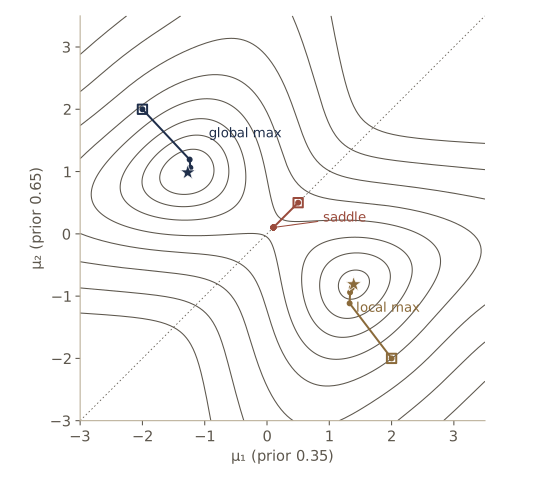
Three different behaviors. From \((-2, 2)\) the iteration reaches the global maximum of the log-likelihood. From \((2, -2)\) it reaches a second local maximum, roughly the first with the roles of the two components exchanged. Because the priors are unequal, this “mirror” solution is not exactly as good: the component with prior 0.65 is now asked to explain the smaller group. And from the symmetric start both means jump in one step to the sample mean of all the data and stay there for many iterations. When the two means are equal, every sample has posterior exactly \(P(\omega_i)\) for class \(i\), so each weighted mean is the plain sample mean. That point is a stationary point of the likelihood, a saddle, and only rounding error in the last digits eventually pushes the iteration off it, which is why after 60 steps it has slid to the mirror peak. Figure 1 shows the whole log-likelihood surface.
Case 2: all parameters unknown
When the means, covariances and priors are all unknown, maximum likelihood has a new problem: the likelihood is unbounded. Take a one-dimensional mixture of \(N(\mu, \sigma^2)\) and \(N(0, 1)\) with equal priors, and set \(\mu = x_1\). The first sample then has density at least \(\frac{1}{2}(2\pi)^{-1/2}\sigma^{-1}\), and every other sample has density at least \(\frac{1}{2}(2\pi)^{-1/2} e^{-x_k^2/2}\) from the second component alone. So the likelihood is at least a constant times \(1/\sigma\), which grows without bound as \(\sigma \to 0\). The global maximum does not exist; the supremum is approached by collapsing a component onto a single sample.
xs = rng.normal(0.0, 1.0, size=25)

def loglik_collapse(x, mu, sigma):
    comp1 = np.log(0.5) + log_normal(x, mu, sigma**2)
    comp2 = np.log(0.5) + log_normal(x, 0.0, 1.0)
    return np.logaddexp(comp1, comp2).sum()

for sigma in [1.0, 1e-1, 1e-2, 1e-4, 1e-8, 1e-16]:
    print(f"sigma = {sigma:6.0e}   l = {loglik_collapse(xs, xs[0], sigma):9.3f}")
sigma =  1e+00   l =   -31.171
sigma =  1e-01   l =   -40.682
sigma =  1e-02   l =   -43.862
sigma =  1e-04   l =   -39.266
sigma =  1e-08   l =   -30.056
sigma =  1e-16   l =   -11.635
At first shrinking \(\sigma\) lowers the likelihood, because the narrow component stops explaining any other sample. But once it only has \(x_1\) left, each factor of ten adds \(\ln 10 \approx 2.3\), forever. These singular solutions are useless as estimates. In practice we look instead for the largest of the finite local maxima, and the conditions for those follow from the general gradient condition.
For the derivation it is convenient to treat the elements of \(\boldsymbol{\Sigma}_i^{-1}\) as the unknowns. The gradient of \(\ln p(\mathbf{x}_k \mid \omega_i, \boldsymbol{\theta}_i)\) with respect to \(\boldsymbol{\mu}_i\) is \(\boldsymbol{\Sigma}_i^{-1}(\mathbf{x}_k - \boldsymbol{\mu}_i)\) as before. For the precision matrix, using \(\partial \ln \lvert \mathbf{A} \rvert / \partial \mathbf{A} = \mathbf{A}^{-1}\) for symmetric \(\mathbf{A}\) and \(\partial(\mathbf{v}^{t}\mathbf{A}\mathbf{v})/\partial \mathbf{A} = \mathbf{v}\mathbf{v}^{t}\),
\[\frac{\partial \ln p(\mathbf{x}_k \mid \omega_i, \boldsymbol{\theta}_i)}{\partial \boldsymbol{\Sigma}_i^{-1}} = \tfrac{1}{2}\left[\boldsymbol{\Sigma}_i - (\mathbf{x}_k - \boldsymbol{\mu}_i)(\mathbf{x}_k - \boldsymbol{\mu}_i)^{t}\right]\](treating the matrix entries as free and symmetrizing; accounting for the fact that only half the off-diagonal entries are independent changes the off-diagonal equations by a factor of 2 and not their solution). Weight these by the posteriors, sum over \(k\), set to zero, and combine with the prior condition. The result is a set of coupled equations with a very readable form.
Result. At a local maximum of the likelihood of a normal mixture,
\[\hat{P}(\omega_i) = \frac{1}{n}\sum_{k} \hat{P}_{ik}, \qquad \hat{\boldsymbol{\mu}}_i = \frac{\sum_k \hat{P}_{ik}\,\mathbf{x}_k}{\sum_k \hat{P}_{ik}}, \qquad \hat{\boldsymbol{\Sigma}}_i = \frac{\sum_k \hat{P}_{ik}\,(\mathbf{x}_k - \hat{\boldsymbol{\mu}}_i)(\mathbf{x}_k - \hat{\boldsymbol{\mu}}_i)^{t}}{\sum_k \hat{P}_{ik}},\]where \(\hat{P}_{ik} = \hat{P}(\omega_i \mid \mathbf{x}_k, \hat{\boldsymbol{\theta}})\) is the posterior computed with the estimated parameters. They are a class frequency, a sample mean and a sample covariance, each with fractional memberships.
Iterating these equations (compute the posteriors from the current parameters, then recompute the parameters from the posteriors) is the expectation–maximization (EM) algorithm for normal mixtures. Intro to ML, module 09 proves that each iteration never decreases the likelihood and derives EM in general; here we implement it and watch it work. Our running two-dimensional data set has three groups of 70, 50 and 40 points with different covariances.
rng2 = np.random.default_rng(1002)
means_true = np.array([[0.0, 0.0], [4.0, 1.0], [1.5, 4.0]])
covs_true = np.array([[[1.0, 0.5], [0.5, 0.8]],
                      [[0.6, -0.3], [-0.3, 1.2]],
                      [[0.9, 0.0], [0.0, 0.4]]])
sizes = [70, 50, 40]
X = np.vstack([rng2.multivariate_normal(m, S, size=k) for m, S, k in zip(means_true, covs_true, sizes)])
y_true = np.repeat(np.arange(3), sizes)          # kept only to check the results
init = X[rng2.choice(len(X), 3, replace=False)]  # c = 3 randomly chosen samples as starting means

def log_gauss(X, mu, Sigma):
    """ln N(x | mu, Sigma) for every row of X, via a Cholesky factor."""
    L = np.linalg.cholesky(Sigma)
    Z = np.linalg.solve(L, (X - mu).T)
    return -0.5 * (Z**2).sum(0) - np.log(np.diag(L)).sum() - 0.5 * X.shape[1] * np.log(2 * np.pi)

def em_gmm(X, P, mu, Sigma, iters):
    n, d = X.shape
    c = len(P)
    lls = []
    for _ in range(iters):
        L = np.column_stack([log_gauss(X, mu[i], Sigma[i]) for i in range(c)]) + np.log(P)
        ll = logsumexp(L, axis=1)
        lls.append(ll.sum())
        R = np.exp(L - ll[:, None])                   # posteriors P(w_i | x_k)
        Nk = R.sum(axis=0)
        P = Nk / n                                    # class frequencies
        mu = (R.T @ X) / Nk[:, None]                  # weighted means
        Sigma = np.array([((R[:, i, None] * (X - mu[i])).T @ (X - mu[i])) / Nk[i] for i in range(c)])
    return P, mu, Sigma, np.array(lls), R

P_em, mu_em, Sigma_em, lls, R_em = em_gmm(X, np.full(3, 1 / 3), init.copy(), np.array([np.eye(2)] * 3), 60)
print("log-likelihood at iterations 0, 1, 2, 5, 10, 20, 59:\n", lls[[0, 1, 2, 5, 10, 20, 59]].round(3))
print("never decreases:", bool(np.all(np.diff(lls) >= -1e-9)))
print("priors", P_em)
print("means\n", mu_em)
log-likelihood at iterations 0, 1, 2, 5, 10, 20, 59:
 [-896.044 -568.719 -557.57  -544.042 -531.782 -531.768 -531.768]
never decreases: True
priors [0.3299 0.2315 0.4385]
means
 [[ 3.9127  1.0721]
 [ 1.5268  4.0937]
 [ 0.1364 -0.0246]]
The estimated priors, 0.33, 0.23 and 0.44 in the order EM happened to label the components, are close to the true proportions \(50/160 \approx 0.31\), \(40/160 = 0.25\) and \(70/160 \approx 0.44\) of the groups they found, and the means are close to the true \((4, 1)\), \((1.5, 4)\) and \((0, 0)\).
Now the singularity in action. Add one far-away sample and give EM a fourth component that starts near it.
X_out = np.vstack([X, [[7.5, 5.5]]])
P4 = np.array([0.3, 0.3, 0.3, 0.1])
mu4 = np.vstack([mu_em, [[7.3, 5.3]]])
Sigma4 = np.vstack([Sigma_em, [np.eye(2)]])
for it in range(6):
    try:
        P4, mu4, Sigma4, ll4, _ = em_gmm(X_out, P4, mu4, Sigma4, 1)
    except np.linalg.LinAlgError as err:
        print(f"iteration {it}: {err}")
        break
    print(f"iteration {it}: l = {ll4[-1]:9.3f}   det(Sigma_4) = {np.linalg.det(Sigma4[3]):.3e}   mu_4 = {mu4[3]}")
iteration 0: l =  -557.907   det(Sigma_4) = 2.203e-03   mu_4 = [7.4254 5.4253]
iteration 1: l =  -536.655   det(Sigma_4) = 1.132e-20   mu_4 = [7.5 5.5]
iteration 2: l =  -516.725   det(Sigma_4) = 0.000e+00   mu_4 = [7.5 5.5]
iteration 3: Matrix is not positive definite
The fourth component takes responsibility for the outlier alone, its mean lands on it, its covariance shrinks to (numerically) zero in two steps, and on the next iteration the Cholesky factorization fails. The log-likelihood rose at every iteration, as EM promises; it was rising toward \(+\infty\).
Watch out. Unconstrained maximum likelihood for normal mixtures has no maximum, and EM can walk into a singular solution, especially with isolated points, small clusters or many components. Common defenses: add a small ridge \(\epsilon\mathbf{I}\) to every covariance estimate, restart a component whose covariance becomes nearly singular, restrict the covariances (diagonal, or one covariance shared by all components, which removes the singularity when there are more samples than dimensions), or place a prior on the covariances and compute a MAP estimate.
The results depend on the starting point, and there may be several local maxima, as in Case 1. Good starting values, for example from a small labeled set or from k-means, help a great deal.
k-means clustering
The posterior \(P(\omega_i \mid \mathbf{x}_k, \hat{\boldsymbol{\theta}})\) is large when the squared Mahalanobis distance from \(\mathbf{x}_k\) to \(\hat{\boldsymbol{\mu}}_i\) is small. A drastic but useful approximation replaces it by an indicator: compute squared Euclidean distances, find the nearest mean \(\hat{\boldsymbol{\mu}}_m\), and set
\[\hat{P}(\omega_i \mid \mathbf{x}_k) \approx \begin{cases} 1 & \text{if } i = m, \\ 0 & \text{otherwise.} \end{cases}\]With hard memberships, the mean update becomes the ordinary mean of the samples currently assigned to each cluster. The resulting procedure is k-means clustering (DHS point out it would be more consistent to call it c-means, since the number of clusters is \(c\); the name k-means is universal):
- choose \(c\) initial means, traditionally \(c\) randomly chosen samples;
- assign each sample to its nearest mean;
- recompute each mean as the average of its samples;
- repeat 2–3 until no assignment changes.
Each pass costs \(O(ndc)\) for the distances, so \(T\) passes cost \(O(ndcT)\), and \(T\) is usually far smaller than \(n\). k-means is also a descent method for the sum-of-squared-error \(J_e = \sum_i \sum_{\mathbf{x} \in \mathcal{D}_i} \lVert \mathbf{x} - \mathbf{m}_i \rVert^2\), where \(\mathcal{D}_i\) is the set of samples in cluster \(i\) and \(\mathbf{m}_i\) its mean. Moving a sample to a nearer mean lowers its term while the means stay fixed, and replacing each mean by its cluster’s average minimizes that cluster’s squared error. Neither step can raise \(J_e\) and there are finitely many partitions, so k-means stops after finitely many passes, at a partition that no single step of either kind can improve (a local minimum in that sense).
def kmeans(X, mu0, max_iter=100):
    mu = mu0.copy()
    history = [mu.copy()]
    for t in range(max_iter):
        z = sq_dists(X, mu).argmin(axis=1)                  # nearest mean
        new = np.array([X[z == i].mean(axis=0) if np.any(z == i) else mu[i] for i in range(len(mu))])
        history.append(new.copy())
        if np.allclose(new, mu):
            break
        mu = new
    return mu, z, history

def J_e(X, z):
    """Sum-of-squared-error criterion of the partition given by labels z."""
    return sum(((X[z == i] - X[z == i].mean(axis=0)) ** 2).sum() for i in np.unique(z))

mu_km, z_km, hist_km = kmeans(X, init)
for t, m in enumerate(hist_km):
    print(f"pass {t}: J_e of nearest-mean partition = {J_e(X, sq_dists(X, m).argmin(axis=1)):.3f}")
print("k-means means\n", mu_km)
print("clusters (rows) vs true groups (columns)\n",
      np.array([[np.sum((z_km == i) & (y_true == j)) for j in range(3)] for i in range(3)]))
pass 0: J_e of nearest-mean partition = 330.431
pass 1: J_e of nearest-mean partition = 227.187
pass 2: J_e of nearest-mean partition = 208.877
pass 3: J_e of nearest-mean partition = 208.877
pass 4: J_e of nearest-mean partition = 208.877
k-means means
 [[ 3.9457  0.9891]
 [ 1.5758  4.0134]
 [ 0.122  -0.0646]]
clusters (rows) vs true groups (columns)
 [[ 1 49  1]
 [ 0  1 39]
 [69  0  0]]
The criterion falls from 330 to 209 in two passes; the third pass moves the means to the centroids of that final partition, and the fourth confirms that nothing changes. The clusters agree with the true groups on 157 of 160 points. Figure 2 shows the path of the means and, next to it, the mixture that EM found from the same start.
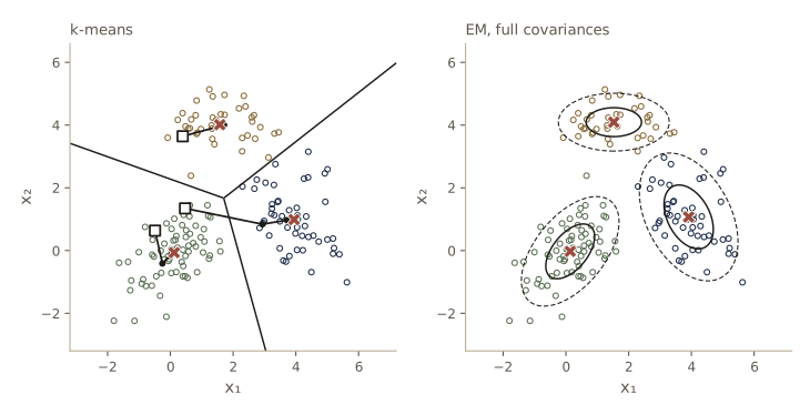
k-means as a limit of EM. Suppose every component has the same covariance \(\sigma^2\mathbf{I}\) and equal priors. Then the posterior is a softmax of \(-\lVert \mathbf{x}_k - \boldsymbol{\mu}_i \rVert^2/(2\sigma^2)\), and as \(\sigma^2 \to 0\) it puts all its weight on the nearest mean: EM’s weighted-mean update becomes the k-means update exactly. The cell measures how far the soft posteriors are from the k-means indicators as \(\sigma^2\) shrinks.
Z_hard = np.eye(3)[z_km]
for sigma2 in [4.0, 1.0, 0.1, 0.01]:
    L = -sq_dists(X, mu_km) / (2 * sigma2)
    R_soft = np.exp(L - logsumexp(L, axis=1, keepdims=True))
    print(f"sigma^2 = {sigma2:5.2f}: max |soft - hard| = {np.abs(R_soft - Z_hard).max():.2e},"
          f" mean largest posterior = {R_soft.max(axis=1).mean():.4f}")
sigma^2 =  4.00: max |soft - hard| = 5.90e-01, mean largest posterior = 0.7581
sigma^2 =  1.00: max |soft - hard| = 4.49e-01, mean largest posterior = 0.9751
sigma^2 =  0.10: max |soft - hard| = 5.06e-02, mean largest posterior = 0.9996
sigma^2 =  0.01: max |soft - hard| = 1.99e-13, mean largest posterior = 1.0000
So k-means is EM for a very particular mixture, with spherical, equal, vanishing covariances. That explains both why it is fast and what it assumes: compact, roughly spherical clusters of similar spread. In the 1-D example of Figure 1, DHS observe that k-means paths climb the same likelihood surface and end near its peaks, and that the two methods agree when the components overlap little.
Fuzzy k-means
k-means puts each sample in exactly one cluster at every step. Fuzzy k-means lets each sample \(\mathbf{x}_j\) have a graded membership \(\hat{P}(\omega_i \mid \mathbf{x}_j)\) in every cluster, with memberships of each sample summing to one, and minimizes the heuristic criterion
\[J_{\text{fuz}} = \sum_{i=1}^{c} \sum_{j=1}^{n} \left[\hat{P}(\omega_i \mid \mathbf{x}_j)\right]^{b} \lVert \mathbf{x}_j - \boldsymbol{\mu}_i \rVert^2, \qquad \sum_{i=1}^{c} \hat{P}(\omega_i \mid \mathbf{x}_j) = 1 \text{ for every } j.\]The fuzziness exponent \(b > 1\) controls how much the clusters blend. (For \(b = 1\) the criterion is linear in the memberships, the minimum puts all of each sample’s weight on its nearest mean, and we are back to the hard assignments of k-means.)
To minimize, fix the memberships and set the gradient with respect to \(\boldsymbol{\mu}_i\) to zero: \(-2\sum_j \hat{P}_{ij}^{b}(\mathbf{x}_j - \boldsymbol{\mu}_i) = \mathbf{0}\), so
\[\boldsymbol{\mu}_i = \frac{\sum_{j} \hat{P}_{ij}^{b}\, \mathbf{x}_j}{\sum_{j} \hat{P}_{ij}^{b}},\]writing \(\hat{P}_{ij}\) for \(\hat{P}(\omega_i \mid \mathbf{x}_j)\). Then fix the means and minimize over the memberships of sample \(j\) with a multiplier \(\lambda_j\) for its sum constraint. With \(d_{ij} = \lVert \mathbf{x}_j - \boldsymbol{\mu}_i \rVert^2\), the derivative of the Lagrangian is \(b\hat{P}_{ij}^{b-1} d_{ij} - \lambda_j = 0\), so \(\hat{P}_{ij} = (\lambda_j / (b\, d_{ij}))^{1/(b-1)}\), proportional to \((1/d_{ij})^{1/(b-1)}\). Normalizing,
\[\hat{P}(\omega_i \mid \mathbf{x}_j) = \frac{(1/d_{ij})^{1/(b-1)}}{\sum_{r=1}^{c} (1/d_{rj})^{1/(b-1)}}.\]Fuzzy k-means alternates these two updates. As \(b \to 1^{+}\) the exponent \(1/(b-1)\) grows and the memberships harden toward k-means; as \(b\) grows they flatten toward \(1/c\).
def fuzzy_kmeans(X, mu0, b, max_iter=200, tol=1e-8):
    mu = mu0.copy()
    for t in range(max_iter):
        d = sq_dists(X, mu) + 1e-12                        # d_ij (rows: samples j, columns: clusters i)
        U = (1.0 / d) ** (1.0 / (b - 1.0))
        U /= U.sum(axis=1, keepdims=True)                  # memberships, each row sums to one
        W = U ** b
        new = (W.T @ X) / W.sum(axis=0)[:, None]           # membership-weighted means
        if np.abs(new - mu).max() < tol:
            break
        mu = new
    return new, U, t + 1

probe = [0, 75, 150]                                       # three samples to follow
print(f"sample positions:\n{X[probe]}")
for b in [1.25, 1.5, 2.0, 3.0]:
    mu_f, U, T = fuzzy_kmeans(X, init, b)
    print(f"b = {b:4.2f} ({T:2d} iterations): mean largest membership {U.max(axis=1).mean():.3f}")
    print(f"    memberships of the three samples: {U[probe].round(2).tolist()}")
sample positions:
[[ 0.5479 -0.8687]
 [ 3.4186  1.5511]
 [ 1.3493  4.2386]]
b = 1.25 (15 iterations): mean largest membership 0.989
    memberships of the three samples: [[0.0, 0.0, 1.0], [1.0, 0.0, 0.0], [0.0, 1.0, 0.0]]
b = 1.50 (17 iterations): mean largest membership 0.964
    memberships of the three samples: [[0.0, 0.0, 1.0], [0.99, 0.01, 0.0], [0.0, 1.0, 0.0]]
b = 2.00 (18 iterations): mean largest membership 0.868
    memberships of the three samples: [[0.05, 0.03, 0.92], [0.88, 0.07, 0.05], [0.01, 0.99, 0.01]]
b = 3.00 (30 iterations): mean largest membership 0.685
    memberships of the three samples: [[0.17, 0.13, 0.7], [0.67, 0.18, 0.15], [0.07, 0.86, 0.07]]
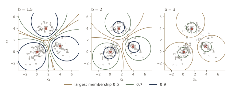
With \(b = 1.25\) the largest membership averages 0.99, so the partition is practically hard; at \(b = 3\) it averages about two thirds, and even the three probe samples, each well inside its own group, give 14 to 33 percent of their membership to the other clusters. Figure 3 shows the largest membership over the whole plane.
A drawback worth knowing: memberships are forced to sum to one over the \(c\) clusters we asked for, so a far-away outlier still gets membership near \(1/c\) in every cluster, and a wrong \(c\) distorts every membership (DHS Computer exercise 4 explores this).
Unsupervised Bayesian learning
Maximum likelihood treats \(\boldsymbol{\theta}\) as fixed but unknown. The Bayesian alternative of module 03 treats it as a random variable with a known prior density \(p(\boldsymbol{\theta})\), and uses the samples to turn the prior into a posterior \(p(\boldsymbol{\theta} \mid \mathcal{D})\). Our assumptions are those of the mixture section (known \(c\), known priors \(P(\omega_j)\), known forms of the component densities) plus a known prior \(p(\boldsymbol{\theta})\), and \(\mathcal{D}\) is a set of \(n\) unlabeled samples drawn independently from the mixture.
The Bayes classifier
To classify a new \(\mathbf{x}\) we need \(P(\omega_i \mid \mathbf{x}, \mathcal{D})\), the posterior given everything we know. By Bayes’ rule, and because nature’s choice of class for the new sample does not depend on the earlier samples, so that \(P(\omega_i \mid \mathcal{D}) = P(\omega_i)\),
\[P(\omega_i \mid \mathbf{x}, \mathcal{D}) = \frac{p(\mathbf{x} \mid \omega_i, \mathcal{D})\, P(\omega_i)}{\sum_{j=1}^{c} p(\mathbf{x} \mid \omega_j, \mathcal{D})\, P(\omega_j)}.\]The class-conditional density given the data is obtained, as in the supervised case, by averaging the model over the posterior of the parameters. The new \(\mathbf{x}\) depends on the data only through \(\boldsymbol{\theta}\), and knowing its class tells us nothing new about \(\boldsymbol{\theta}\), so
\[p(\mathbf{x} \mid \omega_i, \mathcal{D}) = \int p(\mathbf{x} \mid \omega_i, \boldsymbol{\theta}_i)\, p(\boldsymbol{\theta} \mid \mathcal{D})\, d\boldsymbol{\theta}.\]Everything therefore hinges on \(p(\boldsymbol{\theta} \mid \mathcal{D})\).
Learning the parameter vector
Bayes’ rule and independence give
\[p(\boldsymbol{\theta} \mid \mathcal{D}) = \frac{p(\mathcal{D} \mid \boldsymbol{\theta})\, p(\boldsymbol{\theta})}{\int p(\mathcal{D} \mid \boldsymbol{\theta}')\, p(\boldsymbol{\theta}')\, d\boldsymbol{\theta}'}, \qquad p(\mathcal{D} \mid \boldsymbol{\theta}) = \prod_{k=1}^{n} p(\mathbf{x}_k \mid \boldsymbol{\theta}),\]or, writing \(\mathcal{D}^n\) for the first \(n\) samples, in recursive form:
\[p(\boldsymbol{\theta} \mid \mathcal{D}^n) = \frac{p(\mathbf{x}_n \mid \boldsymbol{\theta})\, p(\boldsymbol{\theta} \mid \mathcal{D}^{n-1})}{\int p(\mathbf{x}_n \mid \boldsymbol{\theta}')\, p(\boldsymbol{\theta}' \mid \mathcal{D}^{n-1})\, d\boldsymbol{\theta}'}.\]Each new unlabeled sample multiplies the current posterior by the mixture density evaluated at that sample, and renormalizes. If the prior is roughly flat where the likelihood peaks, and the likelihood has a single sharp peak at \(\hat{\boldsymbol{\theta}}\), then the posterior is sharp at the maximum-likelihood estimate and the integral above collapses to \(p(\mathbf{x} \mid \omega_i, \hat{\boldsymbol{\theta}}_i)\): treating the ML estimate as the true parameter value is then justified. When the likelihood is skewed or has several comparable peaks, as in Figure 1, the two approaches can differ a lot. If the mixture is identifiable, the posterior typically concentrates on the true \(\boldsymbol{\theta}\) as \(n\) grows (DHS Problem 9); if it is not, the posterior may converge to a whole set of parameter values that give the same mixture, and then the components cannot be learned.
Formally this is the supervised recursion of module 03. The difference shows in two places.
No sufficient statistics. Expand the likelihood:
\[p(\mathcal{D} \mid \boldsymbol{\theta}) = \prod_{k=1}^{n} \left[\sum_{j=1}^{c} p(\mathbf{x}_k \mid \omega_j, \boldsymbol{\theta}_j) P(\omega_j)\right].\]Multiplying out gives \(c^n\) terms, one for each way of labeling the \(n\) samples. Parameters and data are thoroughly entangled, the likelihood does not factor into a function of a fixed-size statistic times a function of the data, and the exact posterior must be carried as a function, not as a few numbers.
Diluted evidence. In the supervised case, a sample known to come from \(\omega_1\) multiplies the posterior by the component density \(p(\mathbf{x}_n \mid \omega_1, \boldsymbol{\theta}_1)\). Unlabeled, it multiplies it by the mixture \(\sum_j p(\mathbf{x}_n \mid \omega_j, \boldsymbol{\theta}_j)P(\omega_j)\), in which the other components add terms that do not depend on \(\boldsymbol{\theta}_1\) at all. The sample’s pull on \(\boldsymbol{\theta}_1\) is spread over the classes in proportion to how likely each is to have produced it.
Both points are easy to see in one dimension, where we can represent the posterior on a grid. Our example (not the one in the book) has a known component \(N(-1, 1)\) with prior 0.7 and an unknown component \(N(\theta, 0.7^2)\) with prior 0.3, with true \(\theta = 1.5\). We compare a flat prior on \([-5, 5]\) with a confident but wrong prior \(N(3, 0.5^2)\), and, for reference, the supervised posterior that a teacher who revealed the labels would allow (it uses only the samples from \(\omega_2\)).
rngb = np.random.default_rng(1005)
Pb = np.array([0.7, 0.3])                          # known priors
mu_known, sd_known, sd2, theta_true = -1.0, 1.0, 0.7, 1.5
n_b = 150
labels_b = rngb.choice(2, size=n_b, p=Pb)
xb = np.where(labels_b == 0, rngb.normal(mu_known, sd_known, n_b), rngb.normal(theta_true, sd2, n_b))

theta = np.linspace(-5, 5, 2001)                   # grid for the unknown mean
dth = theta[1] - theta[0]
def npdf(x, m, s):
    return np.exp(-0.5 * ((x - m) / s) ** 2) / (np.sqrt(2 * np.pi) * s)
def normalize(p):
    return p / (p.sum() * dth)
def summary(p):
    m = (theta * p).sum() * dth
    return m, np.sqrt(((theta - m) ** 2 * p).sum() * dth)

post_flat = normalize(np.ones_like(theta))           # uniform prior on [-5, 5]
post_wrong = normalize(npdf(theta, 3.0, 0.5))        # confident, wrong prior
post_sup = post_flat.copy()                          # supervised reference
print("  n  from w2   flat prior: mean   sd   wrong prior: mean   sd   supervised: mean   sd")
for k in range(n_b):
    mix = Pb[0] * npdf(xb[k], mu_known, sd_known) + Pb[1] * npdf(xb[k], theta, sd2)  # p(x_k | theta)
    post_flat = normalize(post_flat * mix)
    post_wrong = normalize(post_wrong * mix)
    if labels_b[k] == 1:
        post_sup = normalize(post_sup * npdf(xb[k], theta, sd2))
    if k + 1 in [1, 2, 5, 10, 25, 50, 150]:
        (a, b), (c_, d_), (e, f) = summary(post_flat), summary(post_wrong), summary(post_sup)
        print(f"{k + 1:3d} {labels_b[:k + 1].sum():6d} {a:16.3f} {b:6.3f} {c_:18.3f} {d_:6.3f} {e:17.3f} {f:6.3f}")
  n  from w2   flat prior: mean   sd   wrong prior: mean   sd   supervised: mean   sd
  1      0           -0.927  2.720              3.000  0.500             0.000  2.888
  2      1            1.349  1.721              2.646  0.426             1.869  0.700
  5      2           -0.071  2.245              2.561  0.453             1.338  0.495
 10      4            1.559  0.414              2.185  0.364             1.583  0.350
 25     11            1.382  0.270              1.787  0.278             1.218  0.211
 50     18            1.533  0.199              1.744  0.198             1.499  0.165
150     47            1.489  0.115              1.567  0.115             1.553  0.102
Read the columns from left to right. The first sample came from the known component, and the flat-prior posterior has changed only a little (a standard deviation of 2.72 against 2.89 for the flat prior itself). For the first few samples the posterior is broad and wanders, because it is not yet clear which samples belong to \(\omega_2\); after 150 samples it has concentrated near 1.49 with standard deviation 0.115. The confident wrong prior holds the estimate up for a while, but the data overwhelm it: by \(n = 150\) the two posteriors differ by less than one posterior standard deviation. The supervised posterior, built from only the 47 samples that came from \(\omega_2\), is narrower still (0.102). Since the standard deviation shrinks like \(0.7/\sqrt{m}\) for \(m\) labeled samples, the 150 unlabeled samples carry about as much information about \(\theta\) as \((0.7/0.115)^2 \approx 37\) labeled ones would. That gap is the price of not knowing the labels.
The recursion hides the \(2^n\) labelings but does not remove them: summing the \(2^{10} = 1024\) labeled terms for the first ten samples gives the same posterior to rounding error. The grid makes the Bayesian answer cheap in one dimension, but a grid over a \(p\)-dimensional \(\boldsymbol{\theta}\) needs a number of points exponential in \(p\), and the exact posterior needs a number of terms exponential in \(n\). That is why approximations are needed.
Decision-directed approximation
The obvious shortcut is to supply the missing labels ourselves: classify each unlabeled sample with the current classifier and then update the parameters as if the decisions were the true labels. This is decision-directed learning. It can run on-line (update after each classified sample) or in batch mode (classify all, update, repeat until the labels stop changing); the batch version with nearest-mean decisions is just k-means.
Its weakness is bias. Even with the true parameters, the decision regions cut the tails off each class: samples from \(\omega_2\) that fall on the \(\omega_1\) side are never used to estimate \(\omega_2\), and samples from \(\omega_1\) in the \(\omega_2\) region are used wrongly. The more the components overlap, the more the estimated means are pushed apart. The simulation estimates \(\theta\) in the model above by batch decision-directed learning and by the maximum-likelihood fixed point of Case 1, for four values of the true \(\theta\) (the closer to \(-1\), the more overlap), starting both at the true value, 100 data sets of 200 samples each.
def decision_directed(x, th, iters=50):
    for _ in range(iters):
        say_w2 = np.log(Pb[1] * npdf(x, th, sd2)) > np.log(Pb[0] * npdf(x, mu_known, sd_known))
        new = x[say_w2].mean()                         # mean of the samples we *decided* are from w2
        if abs(new - th) < 1e-10:
            break
        th = new
    return th

def ml_theta(x, th, iters=100):
    for _ in range(iters):
        a, b = Pb[0] * npdf(x, mu_known, sd_known), Pb[1] * npdf(x, th, sd2)
        r = b / (a + b)                                # P(w2 | x_k, theta)
        th = (r * x).sum() / r.sum()
    return th

rngd = np.random.default_rng(1006)
print("true theta   decision-directed bias (sd)   maximum-likelihood bias (sd)")
for tt in [4.0, 2.5, 1.5, 0.8]:
    dd, ml = [], []
    for rep in range(100):
        l = rngd.choice(2, size=200, p=Pb)
        x = np.where(l == 0, rngd.normal(mu_known, sd_known, 200), rngd.normal(tt, sd2, 200))
        dd.append(decision_directed(x, tt) - tt)
        ml.append(ml_theta(x, tt) - tt)
    print(f"{tt:10.1f} {np.mean(dd):16.3f} ({np.std(dd):.3f}) {np.mean(ml):20.3f} ({np.std(ml):.3f})")
true theta   decision-directed bias (sd)   maximum-likelihood bias (sd)
       4.0           -0.003 (0.093)               -0.002 (0.091)
       2.5            0.003 (0.091)               -0.011 (0.096)
       1.5            0.071 (0.101)               -0.022 (0.110)
       0.8            0.267 (0.092)                0.001 (0.119)
With well-separated components the two estimates agree. As the overlap grows the decision-directed estimate drifts upward, away from the other component, while the ML estimate shows no systematic bias (its average errors stay within about two standard errors of zero). The decision-directed method is still attractive because it is cheap, and it works well when the parametric model is right, the overlap is small and the initial classifier is roughly correct. If the initial classifier is poor, the errors it makes feed back into its training and can lock it into a bad solution (DHS Computer exercise 7).
Data description and clustering
Step back from mixtures. If we knew the samples came from one normal density, the sample mean and covariance would say all there is to say: the mean is the single point closest (in total squared distance) to all the samples, and the covariance describes the spread in each direction. For other shapes those two statistics can be badly misleading: a single blob, two separate blobs, a ring and a pair of parallel lines can all be linearly transformed to have exactly the same sample mean and covariance (try it: whiten each set, then apply one common linear map). A description by first and second moments cannot tell them apart. A mixture of several normal components can describe much more, but fitting mixtures is hard, as we saw, and assuming a parametric form we have no reason to believe risks imposing structure on the data rather than finding it. The nonparametric density estimates of module 04 are another route: the modes of an estimated density suggest groups.
The most direct route is a clustering procedure: describe the data by groups of samples that are more similar to each other than to samples in other groups. Two questions must be answered before any algorithm: how to measure the similarity of two samples, and how to score a proposed partition of the whole set. The next two sections take them in turn.
Similarity measures
The obvious dissimilarity is distance. If distance is a good measure, samples in the same cluster should be closer to each other than to samples in other clusters. The simplest clustering rule follows: join two samples whenever their distance is below a threshold \(d_0\), and call the connected groups clusters. The whole outcome depends on \(d_0\). Too large and everything is one cluster, too small and every sample is its own cluster; natural clusters appear only when \(d_0\) lies between the typical within-cluster and between-cluster distances. On our three-group data:
def connected_components(n, edges):
    """Labels 0, 1, ... of the connected components of a graph on n nodes (union-find)."""
    parent = list(range(n))
    def find(a):
        while parent[a] != a:
            parent[a] = parent[parent[a]]
            a = parent[a]
        return a
    for i, j in edges:
        parent[find(i)] = find(j)
    roots = np.array([find(i) for i in range(n)])
    return np.unique(roots, return_inverse=True)[1]

D_X = pdist(X)
for d0 in [0.3, 0.5, 0.7, 0.8, 1.0, 1.3]:
    edges = list(zip(*np.nonzero(np.triu(D_X < d0, k=1))))
    lab = connected_components(len(X), edges)
    sizes_d0 = np.sort(np.bincount(lab))[::-1]
    print(f"d0 = {d0:3.1f}: {len(sizes_d0):3d} clusters, largest sizes {sizes_d0[:4].tolist()}")
d0 = 0.3:  55 clusters, largest sizes [38, 23, 9, 7]
d0 = 0.5:  17 clusters, largest sizes [66, 37, 22, 13]
d0 = 0.7:  10 clusters, largest sizes [67, 44, 38, 4]
d0 = 0.8:   7 clusters, largest sizes [84, 67, 4, 2]
d0 = 1.0:   2 clusters, largest sizes [90, 70]
d0 = 1.3:   1 clusters, largest sizes [160]
Only a narrow band of thresholds works. At \(d_0 = 0.7\) the three largest components are essentially the three groups (sizes 67, 44 and 38), with a few stray samples on their own; at 0.8 two groups have already joined through a couple of samples lying between them, and from 1.3 on everything is one cluster.
Euclidean distance and scale. Clusters defined by Euclidean distance do not change if we translate or rotate the data. They do change under other linear maps, and in particular under a change of units for one feature. The data below form four blobs at the corners of a 4-by-2 rectangle. With \(c = 2\), the best k-means partition (over several restarts) pairs the corners into a left and a right group. Measure \(x_2\) in units three times smaller, so the rectangle becomes 4 by 6, and the best partition pairs them into a bottom and a top group instead.
def kmeans_best(X, c, rng, restarts=10):
    """Best (lowest J_e) of several k-means runs from random samples."""
    best = (np.inf, None, None)
    for _ in range(restarts):
        mu, z, _ = kmeans(X, X[rng.choice(len(X), c, replace=False)])
        if J_e(X, z) < best[0]:
            best = (J_e(X, z), mu, z)
    return best

rngs = np.random.default_rng(1008)
corners = np.array([[0, 0], [4, 0], [0, 2], [4, 2]], dtype=float)
X_rect = np.vstack([rngs.normal(cn, 0.4, size=(25, 2)) for cn in corners])
corner_of = np.repeat(np.arange(4), 25)
print("corners: 0 bottom left, 1 bottom right, 2 top left, 3 top right")
for scale in [1.0, 3.0]:
    Xs_ = X_rect * np.array([1.0, scale])
    Je_best, mu_s, z_s = kmeans_best(Xs_, 2, rngs)
    groups = [sorted(set(corner_of[z_s == i].tolist())) for i in range(2)]
    print(f"x2 scaled by {scale}: corners grouped as {groups}")
corners: 0 bottom left, 1 bottom right, 2 top left, 3 top right
x2 scaled by 1.0: corners grouped as [[0, 2], [1, 3]]
x2 scaled by 3.0: corners grouped as [[0, 1], [2, 3]]
Neither answer is wrong. They are answers to different questions, because the units are part of the question. One common response is to standardize each feature to zero mean and unit variance before clustering, and perhaps to rotate to principal axes first. That is appropriate when the spread of a feature is random noise. It is harmful when the spread is caused by the very clusters we are looking for: a feature that separates two groups widely has a large variance for that reason, and dividing by it shrinks the separation. Clusters should be invariant to transformations that are natural to the problem, and only the designer can say which ones those are.
Other metrics. The Minkowski metric
\[d_q(\mathbf{x}, \mathbf{x}') = \left(\sum_{i=1}^{d} \lvert x_i - x'_i \rvert^{q}\right)^{1/q}, \qquad q \ge 1,\]gives the Euclidean distance for \(q = 2\) and the city-block (Manhattan) distance for \(q = 1\); among these only \(q = 2\) is unchanged by rotations. The Mahalanobis distance \(\sqrt{(\mathbf{x} - \mathbf{x}')^{t}\boldsymbol{\Sigma}^{-1}(\mathbf{x} - \mathbf{x}')}\), with \(\boldsymbol{\Sigma}\) estimated from the data, uses the data’s own covariance to set the scale. It is invariant to every nonsingular linear transformation of the features, but if \(\boldsymbol{\Sigma}\) is the covariance of all the data it again mixes cluster structure into the “noise” (the standardization problem in matrix form).
Similarity functions. We can also drop the idea of a metric and use a similarity function \(s(\mathbf{x}, \mathbf{x}')\), symmetric and large when the two samples are alike. When direction matters more than length, the cosine of the angle,
\[s(\mathbf{x}, \mathbf{x}') = \frac{\mathbf{x}^{t}\mathbf{x}'}{\lVert \mathbf{x} \rVert\, \lVert \mathbf{x}' \rVert},\]is natural; it is invariant to rotations and to rescaling of either vector, but not to translations. For binary features, where \(x_i = 1\) means “has attribute \(i\)”, \(\mathbf{x}^{t}\mathbf{x}'\) counts the attributes both samples have. Dividing by \(d\) gives the fraction of attributes shared, and dividing by the number of attributes that at least one of them has gives the Tanimoto coefficient
\[s_T(\mathbf{x}, \mathbf{x}') = \frac{\mathbf{x}^{t}\mathbf{x}'}{\mathbf{x}^{t}\mathbf{x} + \mathbf{x}'^{t}\mathbf{x}' - \mathbf{x}^{t}\mathbf{x}'},\]widely used in information retrieval and chemistry. The difference matters when most attributes are absent from most samples: shared absences say little, and the Tanimoto coefficient ignores them.
def tanimoto(a, b):
    return a @ b / (a @ a + b @ b - a @ b)

u = np.array([1, 1, 0, 0, 0, 0, 0, 0, 0, 1], dtype=float)
v = np.array([1, 0, 0, 0, 0, 0, 0, 0, 0, 1], dtype=float)
w = np.array([0, 0, 1, 1, 0, 0, 0, 0, 0, 0], dtype=float)
for name, (p, q) in {"u,v": (u, v), "u,w": (u, w)}.items():
    print(f"{name}: shared/d = {p @ q / len(p):.2f}, matches/d = {np.mean(p == q):.2f}, Tanimoto = {tanimoto(p, q):.2f}")
u,v: shared/d = 0.20, matches/d = 0.90, Tanimoto = 0.67
u,w: shared/d = 0.00, matches/d = 0.50, Tanimoto = 0.00
Counting matches (including shared zeros) says that \(\mathbf{u}\) and \(\mathbf{w}\) agree on half of the ten attributes, although they have no attribute in common; Tanimoto gives them zero and gives \(\mathbf{u}, \mathbf{v}\) two thirds. Features that mix meters, kilograms and categories raise questions that no formula answers. Whatever similarity we choose puts the designer’s knowledge into the procedure, and the same similarity should later be used to classify new samples into the clusters.
Criterion functions for clustering
Now the second question. We want to partition \(\mathcal{D}\) into exactly \(c\) disjoint subsets \(\mathcal{D}_1, \dots, \mathcal{D}_c\) so that samples in the same subset are more alike than samples in different subsets. A criterion function assigns a number to every partition, and the best partition is the one that extremizes it. This section compares several criteria; the next two describe how to search for good partitions.
The sum-of-squared-error criterion
Let \(n_i\) be the number of samples in \(\mathcal{D}_i\) and \(\mathbf{m}_i = \frac{1}{n_i}\sum_{\mathbf{x} \in \mathcal{D}_i} \mathbf{x}\) their mean. The sum-of-squared-error criterion is
\[J_e = \sum_{i=1}^{c} \sum_{\mathbf{x} \in \mathcal{D}_i} \lVert \mathbf{x} - \mathbf{m}_i \rVert^2 .\]Within each cluster the mean is the point that minimizes the sum of squared distances to its members, so \(J_e\) is the total squared error of representing every sample by the center of its cluster. Partitions that minimize it are called minimum-variance partitions. The criterion suits compact, well-separated clouds of similar size.
A little algebra removes the means. Expand \(\lVert \mathbf{x} - \mathbf{x}' \rVert^2 = \lVert (\mathbf{x} - \mathbf{m}_i) - (\mathbf{x}' - \mathbf{m}_i) \rVert^2\) and sum over all ordered pairs in \(\mathcal{D}_i\); the cross terms vanish because deviations from the mean sum to zero, leaving \(\sum_{\mathbf{x}, \mathbf{x}' \in \mathcal{D}_i} \lVert \mathbf{x} - \mathbf{x}' \rVert^2 = 2 n_i \sum_{\mathbf{x} \in \mathcal{D}_i} \lVert \mathbf{x} - \mathbf{m}_i \rVert^2\). Hence
\[J_e = \frac{1}{2} \sum_{i=1}^{c} n_i\, \bar{s}_i, \qquad \bar{s}_i = \frac{1}{n_i^2} \sum_{\mathbf{x} \in \mathcal{D}_i} \sum_{\mathbf{x}' \in \mathcal{D}_i} \lVert \mathbf{x} - \mathbf{x}' \rVert^2 .\]So \(J_e\) is really a statement about pairwise squared Euclidean distances within clusters, \(\bar{s}_i\) being their average. This form suggests a family of related minimum-variance criteria: replace \(\bar{s}_i\) by the median or maximum pairwise distance, or by an average or minimum of any similarity \(s(\mathbf{x}, \mathbf{x}')\) over pairs in the cluster (to be maximized, for a similarity).
z = z_km
pairwise_form = 0.5 * sum((z == i).sum() * sq_dists(X[z == i], X[z == i]).sum() / (z == i).sum() ** 2
                          for i in range(3))
print(f"J_e from the means: {J_e(X, z):.4f}   from pairwise distances: {pairwise_form:.4f}")

# J_e and very unequal cluster sizes
rngu = np.random.default_rng(1009)
X_big = rngu.normal([0, 0], 1.0, size=(200, 2))
X_small = rngu.normal([4.5, 0], 0.4, size=(10, 2))
X_u = np.vstack([X_big, X_small])
natural = np.r_[np.zeros(200, int), np.ones(10, int)]
Je_km, mu_u, z_u = kmeans_best(X_u, 2, rngu)
print(f"natural partition (200 + 10): J_e = {J_e(X_u, natural):.1f}")
print(f"best k-means partition, sizes {np.bincount(z_u).tolist()}: J_e = {Je_km:.1f}")
print(f"all 10 points of the small group in the same cluster: {len(set(z_u[200:].tolist())) == 1}")
J_e from the means: 208.8774   from pairwise distances: 208.8774
natural partition (200 + 10): J_e = 407.0
best k-means partition, sizes [150, 60]: J_e = 386.6
all 10 points of the small group in the same cluster: True
The second part of the cell shows the classic failure. A cloud of 200 points and a tight group of 10 are obviously two clusters, yet slicing off about a quarter of the big cloud (50 points) and putting the small group in with that slice gives a smaller \(J_e\). With sizes this unequal, the reduction from splitting the big cloud outweighs the cost of lumping the small group with its neighbors.
Watch out. \(J_e\) prefers clusters of similar size and similar spread. A large diffuse cluster next to a small compact one, or a few outliers, can make a partition that splits the large cluster score better than the natural one. When such effects make the minimizer of \(J_e\) unacceptable, that knowledge should be built into a different criterion rather than patched afterward.
Scatter matrices
The scatter matrices of Fisher’s multiple discriminant analysis (module 03; DHS §3.8) give another family of criteria. With \(\mathbf{m}\) the mean of all \(n\) samples, define
\[\begin{aligned} \mathbf{S}_i &= \sum_{\mathbf{x} \in \mathcal{D}_i} (\mathbf{x} - \mathbf{m}_i)(\mathbf{x} - \mathbf{m}_i)^{t} && \text{scatter matrix of cluster } i, \\ \mathbf{S}_W &= \sum_{i=1}^{c} \mathbf{S}_i && \text{within-cluster scatter,} \\ \mathbf{S}_B &= \sum_{i=1}^{c} n_i (\mathbf{m}_i - \mathbf{m})(\mathbf{m}_i - \mathbf{m})^{t} && \text{between-cluster scatter,} \\ \mathbf{S}_T &= \sum_{\mathbf{x} \in \mathcal{D}} (\mathbf{x} - \mathbf{m})(\mathbf{x} - \mathbf{m})^{t} && \text{total scatter.} \end{aligned}\]Writing \(\mathbf{x} - \mathbf{m} = (\mathbf{x} - \mathbf{m}_i) + (\mathbf{m}_i - \mathbf{m})\) inside \(\mathbf{S}_T\) and summing over each cluster, the cross terms vanish (deviations from \(\mathbf{m}_i\) sum to zero within cluster \(i\)), so
\[\mathbf{S}_T = \mathbf{S}_W + \mathbf{S}_B .\]\(\mathbf{S}_T\) does not depend on the partition at all. Whatever within-cluster scatter a partition removes is converted into between-cluster scatter, so minimizing the one and maximizing the other are two views of the same goal. To turn a matrix into a criterion we need a scalar measure of its size.
The trace criterion. The trace is the sum of the variances along the coordinate axes, a squared scattering radius. And
\[\operatorname{tr} \mathbf{S}_W = \sum_{i} \sum_{\mathbf{x} \in \mathcal{D}_i} \lVert \mathbf{x} - \mathbf{m}_i \rVert^2 = J_e,\]so minimizing the trace of \(\mathbf{S}_W\) is the sum-of-squared-error criterion again. Since \(\operatorname{tr}\mathbf{S}_T\) is fixed, it is also the same as maximizing \(\operatorname{tr}\mathbf{S}_B = \sum_i n_i \lVert \mathbf{m}_i - \mathbf{m} \rVert^2\).
The determinant criterion. The determinant is the product of the variances along the principal axes, a squared scattering volume. \(\mathbf{S}_B\) has rank at most \(c - 1\), so its determinant is zero whenever \(c \le d\) and is useless. But \(\mathbf{S}_W\) is usually nonsingular (it is certainly singular if \(n - c < d\)), which gives the determinant criterion
\[J_d = \lvert \mathbf{S}_W \rvert = \left\lvert \sum_{i=1}^{c} \mathbf{S}_i \right\rvert .\]Its great property is invariance. Under a nonsingular linear change of coordinates \(\mathbf{x} \mapsto \mathbf{A}\mathbf{x} + \mathbf{b}\), every scatter matrix becomes \(\mathbf{A}\mathbf{S}\mathbf{A}^{t}\), so \(J_d\) is multiplied by \(\lvert \mathbf{A} \rvert^2\) for every partition alike, and the best partition does not change. \(J_e\) has no such property, as the rectangle example showed.
Invariant criteria. Under the same change of coordinates, \(\mathbf{S}_W^{-1}\mathbf{S}_B\) becomes \((\mathbf{A}\mathbf{S}_W\mathbf{A}^{t})^{-1}\mathbf{A}\mathbf{S}_B\mathbf{A}^{t} = \mathbf{A}^{-t}\,\mathbf{S}_W^{-1}\mathbf{S}_B\,\mathbf{A}^{t}\), a similar matrix, so its eigenvalues \(\lambda_1, \dots, \lambda_d\) do not change. They are the fundamental linear invariants of the scatter matrices: each measures between-cluster scatter relative to within-cluster scatter along one direction, and at most \(c - 1\) of them are nonzero. Good partitions make them large, and any function of them gives an invariant criterion. Because \(\mathbf{S}_W^{-1}\mathbf{S}_T = \mathbf{I} + \mathbf{S}_W^{-1}\mathbf{S}_B\) has eigenvalues \(1 + \lambda_i\),
Result. For \(\lambda_1, \dots, \lambda_d\) the eigenvalues of \(\mathbf{S}_W^{-1}\mathbf{S}_B\),
\[\operatorname{tr}\left(\mathbf{S}_W^{-1}\mathbf{S}_B\right) = \sum_{i=1}^{d} \lambda_i, \qquad \operatorname{tr}\left(\mathbf{S}_T^{-1}\mathbf{S}_W\right) = \sum_{i=1}^{d} \frac{1}{1 + \lambda_i}, \qquad \frac{\lvert \mathbf{S}_W \rvert}{\lvert \mathbf{S}_T \rvert} = \prod_{i=1}^{d} \frac{1}{1 + \lambda_i}.\]The first is maximized, the other two minimized. All three, and the partitions that optimize them, are invariant to nonsingular linear transformations. Since \(\lvert \mathbf{S}_T \rvert\) is fixed, the third ranks partitions exactly as \(J_d\) does.
With two clusters only \(\lambda_1\) can be nonzero, and every one of these criteria is a monotonic function of it: for \(c = 2\), \(J_d\) and all the invariant criteria pick the same partition. With more clusters they can differ. One more remark from DHS: \(\operatorname{tr}(\mathbf{S}_T^{-1}\mathbf{S}_W)\) is \(J_e\) computed after transforming the data so that \(\mathbf{S}_T = \mathbf{I}\), which is exactly the whole-data standardization we warned about, so it inherits its flaws.
Let us verify the identities, then do what is rarely possible: find the exact optimum of each criterion by trying every partition. With \(n = 12\) samples there are 2,047 ways to split them into two nonempty clusters and 86,526 ways to split them into three (the Stirling numbers of the second kind), few enough to enumerate with vectorized NumPy. The data are 12 points from a single elongated Gaussian, with no real cluster structure, which is exactly when criteria are most likely to disagree.
def scatter_matrices(X, z):
    m = X.mean(axis=0)
    S_W = sum((X[z == i] - X[z == i].mean(0)).T @ (X[z == i] - X[z == i].mean(0)) for i in np.unique(z))
    S_B = sum((z == i).sum() * np.outer(X[z == i].mean(0) - m, X[z == i].mean(0) - m) for i in np.unique(z))
    S_T = (X - m).T @ (X - m)
    return S_W, S_B, S_T

S_W, S_B, S_T = scatter_matrices(X, z_km)
lam = np.linalg.eigvals(np.linalg.solve(S_W, S_B)).real
print(f"S_T - S_W - S_B = {np.abs(S_T - S_W - S_B).max():.1e};  tr S_W = {np.trace(S_W):.4f} = J_e = {J_e(X, z_km):.4f}")
print(f"tr(S_T^-1 S_W) = {np.trace(np.linalg.solve(S_T, S_W)):.4f}, sum 1/(1+lambda) = {np.sum(1 / (1 + lam)):.4f}")
A_lin = np.array([[2.0, 1.0], [-0.5, 3.0]])
S_W2, S_B2, _ = scatter_matrices(X @ A_lin.T + np.array([5.0, -1.0]), z_km)
lam2 = np.linalg.eigvals(np.linalg.solve(S_W2, S_B2)).real
print(f"eigenvalues of S_W^-1 S_B: {np.sort(lam)} before, {np.sort(lam2)} after a linear map")
print(f"|S_W| ratio after/before = {np.linalg.det(S_W2) / np.linalg.det(S_W):.4f}, |A|^2 = {np.linalg.det(A_lin) ** 2:.4f}")
S_T - S_W - S_B = 2.8e-14;  tr S_W = 208.8774 = J_e = 208.8774
tr(S_T^-1 S_W) = 0.4007, sum 1/(1+lambda) = 0.4007
eigenvalues of S_W^-1 S_B: [3.5016 4.6005] before, [3.5016 4.6005] after a linear map
|S_W| ratio after/before = 42.2500, |A|^2 = 42.2500
For the exhaustive search we represent each partition by a label vector whose first sample is in cluster 0, whose first sample not in cluster 0 is in cluster 1, and so on, so that each partition appears once. All the scatter matrices come from sums of \(\mathbf{x}\mathbf{x}^{t}\) over each cluster, which vectorize well: \(\mathbf{S}_W = \sum_{\mathbf{x}} \mathbf{x}\mathbf{x}^{t} - \sum_i \frac{1}{n_i}\mathbf{s}_i\mathbf{s}_i^{t}\) with \(\mathbf{s}_i\) the sum of the samples in cluster \(i\).
def all_partitions(n, c):
    """Label vectors of every partition of n samples into c nonempty clusters, each partition once."""
    Z = np.array(list(itertools.product(range(c), repeat=n - 1)), dtype=np.int8)
    Z = np.column_stack([np.zeros(len(Z), np.int8), Z])
    present = np.stack([(Z == k).any(axis=1) for k in range(c)], axis=1)
    first = np.stack([np.where(present[:, k], (Z == k).argmax(axis=1), n) for k in range(c)], axis=1)
    return Z[present.all(axis=1) & np.all(np.diff(first, axis=1) > 0, axis=1)]

def all_criteria(X, Z, c):
    """J_e, J_d, -tr(S_W^-1 S_B) and tr(S_T^-1 S_W) for every partition, all to be minimized."""
    S_W = np.broadcast_to(X.T @ X, (len(Z), X.shape[1], X.shape[1])).copy()
    for k in range(c):
        M = (Z == k).astype(float)
        s = M @ X                                             # sum of the samples in cluster k
        S_W -= s[:, :, None] * s[:, None, :] / M.sum(axis=1)[:, None, None]
    S_T = (X - X.mean(0)).T @ (X - X.mean(0))
    S_B = S_T - S_W
    return {"J_e": np.trace(S_W, axis1=1, axis2=2),
            "J_d": np.linalg.det(S_W),
            "trWB": -np.trace(np.linalg.solve(S_W, S_B), axis1=1, axis2=2),   # maximize tr(S_W^-1 S_B)
            "trTW": np.trace(np.linalg.solve(S_T, S_W), axis1=1, axis2=2)}    # minimize tr(S_T^-1 S_W)

rngc = np.random.default_rng(9)
X12 = np.round(rngc.normal(size=(12, 2)) * np.array([1.2, 0.7]), 2)
A_stretch = np.array([[3.0, 0.0], [1.0, 0.5]])
for c in [2, 3]:
    Z = all_partitions(12, c)
    print(f"c = {c}: {len(Z)} partitions")
    for name, data in [("original", X12), ("x -> Ax", X12 @ A_stretch.T)]:
        best = {k: "".join("ABC"[i] for i in Z[v.argmin()]) for k, v in all_criteria(data, Z, c).items()}
        print(f"  {name:8s}", "  ".join(f"{k} {v}" for k, v in best.items()))
c = 2: 2047 partitions
  original J_e AABBBAABAABA  J_d ABAAABBABBAB  trWB ABAAABBABBAB  trTW ABAAABBABBAB
  x -> Ax  J_e AABBAABBAAAA  J_d ABAAABBABBAB  trWB ABAAABBABBAB  trTW ABAAABBABBAB
c = 3: 86526 partitions
  original J_e ABCCABACAAAB  J_d AABBAACBBBAB  trWB ABCCABACAAAB  trTW AABBAACBCCAC
  x -> Ax  J_e ABCCABACAAAB  J_d AABBAACBBBAB  trWB ABCCABACAAAB  trTW AABBAACBCCAC
Each string gives the cluster (A, B or C) of the 12 samples in order; trWB and trTW stand for the two trace criteria of the box above. For \(c = 2\), \(J_d\) and the two invariant criteria pick the same partition, as the theory says, and \(J_e\) picks a different one. After stretching and shearing the data with \(\mathbf{A}\), \(J_e\) changes its mind while the others do not move. For \(c = 3\) the four criteria produce three different optimal partitions (here \(J_e\) and \(\operatorname{tr}\mathbf{S}_W^{-1}\mathbf{S}_B\) happen to agree). This particular map happens not to change the \(J_e\) optimum for \(c = 3\); for the other three criteria that is guaranteed, for \(J_e\) it is luck.
Two cautions. First, invariance cuts both ways: if different linear transformations of the data would reveal different groupings, an invariant criterion sees all of them at once, and it tends to have more local optima, which makes it harder to optimize. Second, all of these criteria share one picture of a cluster: a compact cloud measured by \(\mathbf{S}_W\). None of them will pull a dense cluster out of the middle of a diffuse one, or separate two interleaved curved or elongated clusters. Such structure needs a different criterion, or one of the graph-based methods below.
Iterative optimization
Once a criterion is fixed, clustering is a discrete optimization problem over a finite set of partitions, so in principle we could search them all, as we just did for 12 points. In practice the count explodes: the number of partitions of \(n\) samples into \(c\) nonempty clusters is the Stirling number of the second kind \(S(n, c) = \frac{1}{c!}\sum_{j=0}^{c} (-1)^j \binom{c}{j}(c - j)^n\), roughly \(c^n/c!\) for large \(n\). It was 86,526 for our 12 points and 3 clusters; for 100 samples and 5 clusters it is about \(6.6 \times 10^{67}\). So we use iterative optimization: start from some partition and keep moving samples between clusters while each move improves the criterion. Like any hill climbing it finds a local optimum that depends on the start.
For \(J_e\) the effect of moving one sample can be computed without recomputing anything else. Write \(J_i = \sum_{\mathbf{x} \in \mathcal{D}_i} \lVert \mathbf{x} - \mathbf{m}_i \rVert^2\) so that \(J_e = \sum_i J_i\). Suppose sample \(\hat{\mathbf{x}}\), now in \(\mathcal{D}_i\), is moved to \(\mathcal{D}_j\). The mean of \(\mathcal{D}_j\) becomes \(\mathbf{m}_j^* = \mathbf{m}_j + (\hat{\mathbf{x}} - \mathbf{m}_j)/(n_j + 1)\). For the old members, \(\sum \lVert \mathbf{x} - \mathbf{m}_j^* \rVert^2 = J_j + n_j \lVert \mathbf{m}_j^* - \mathbf{m}_j \rVert^2\) (the cross term vanishes again), and the newcomer contributes \(\lVert \hat{\mathbf{x}} - \mathbf{m}_j^* \rVert^2 = \left(\frac{n_j}{n_j + 1}\right)^2 \lVert \hat{\mathbf{x}} - \mathbf{m}_j \rVert^2\). Adding,
\[J_j^* = J_j + \frac{n_j}{(n_j + 1)^2}\lVert \hat{\mathbf{x}} - \mathbf{m}_j \rVert^2 + \frac{n_j^2}{(n_j + 1)^2}\lVert \hat{\mathbf{x}} - \mathbf{m}_j \rVert^2 = J_j + \frac{n_j}{n_j + 1} \lVert \hat{\mathbf{x}} - \mathbf{m}_j \rVert^2 .\]The same calculation in reverse (valid if \(n_i > 1\); we never empty a cluster) gives
\[J_i^* = J_i - \frac{n_i}{n_i - 1} \lVert \hat{\mathbf{x}} - \mathbf{m}_i \rVert^2 .\]So the transfer lowers \(J_e\) exactly when
\[\frac{n_j}{n_j + 1} \lVert \hat{\mathbf{x}} - \mathbf{m}_j \rVert^2 < \frac{n_i}{n_i - 1} \lVert \hat{\mathbf{x}} - \mathbf{m}_i \rVert^2 ,\]and among all target clusters the best is the one with the smallest \(\frac{n_j}{n_j + 1}\lVert \hat{\mathbf{x}} - \mathbf{m}_j \rVert^2\). This is usually, but not always, the cluster with the nearest mean: the size factors make leaving a small cluster especially profitable and joining a small cluster comparatively cheap. The resulting sequential minimum-squared-error procedure picks samples one at a time, transfers each when that helps, and updates the two affected means immediately. It is a sequential cousin of k-means, which reassigns all samples before recomputing any mean.
def transfer_pass(X, z, rng):
    """One pass of single-sample transfers that lower J_e; returns labels, number of moves."""
    z = z.copy()
    c = z.max() + 1
    n_c = np.bincount(z, minlength=c).astype(float)
    m = np.array([X[z == i].mean(axis=0) for i in range(c)])
    moves = 0
    for k in rng.permutation(len(X)):
        i = z[k]
        if n_c[i] == 1:
            continue                                   # never destroy a singleton
        d2 = ((X[k] - m) ** 2).sum(axis=1)
        rho = n_c / (n_c + 1) * d2                     # increase of J_j if moved to j
        rho[i] = n_c[i] / (n_c[i] - 1) * d2[i]         # decrease of J_i if moved out of i
        j = int(np.argmin(rho))
        if j != i:
            predicted = rho[j] - rho[i]
            before = J_e(X, z)
            m[i] -= (X[k] - m[i]) / (n_c[i] - 1)       # update both means and counts
            m[j] += (X[k] - m[j]) / (n_c[j] + 1)
            n_c[i] -= 1; n_c[j] += 1
            z[k] = j
            moves += 1
            if moves == 1:
                print(f"first transfer: predicted change {predicted:.4f}, actual {J_e(X, z) - before:.4f}")
    return z, moves

rngt = np.random.default_rng(1010)
z_it = sq_dists(X, init).argmin(axis=1)                # start from the nearest-initial-mean partition
print(f"start: J_e = {J_e(X, z_it):.3f}")
for p in range(5):
    z_it, moves = transfer_pass(X, z_it, rngt)
    print(f"pass {p + 1}: {moves:3d} transfers, J_e = {J_e(X, z_it):.3f}")
    if moves == 0:
        break
print(f"k-means from the same start: J_e = {J_e(X, z_km):.3f}")
start: J_e = 330.431
first transfer: predicted change -0.5535, actual -0.5535
pass 1:  24 transfers, J_e = 216.674
first transfer: predicted change -4.0389, actual -4.0389
pass 2:   2 transfers, J_e = 208.877
pass 3:   0 transfers, J_e = 208.877
k-means from the same start: J_e = 208.877
The predicted change matches the recomputed one, and the procedure settles at the same partition k-means found. At a k-means fixed point each sample is nearest its own mean, but the transfer test also accounts for how the two means move, so the sequential procedure can sometimes improve a k-means solution further (Exercise 5). Its drawbacks are that its result depends on the order in which samples are visited and that it is, if anything, more prone to local minima. Its advantage is that it is stepwise optimal and naturally on-line.
The starting point matters for every hill climber. Options include several random starts, or growing the solution: the one-cluster solution is the overall mean, and a \(c\)-cluster start can be the \((c-1)\)-cluster means plus the sample farthest from its nearest mean. Building partitions for every \(c\) in sequence leads naturally to hierarchical clustering.
Hierarchical clustering
The partitions so far are flat. Many data sets have groups inside groups (biological taxonomy is the textbook case: kingdom, phylum, class, order, family, genus, species), and a single number of clusters misses that structure.
Definitions
Consider a sequence of partitions of the \(n\) samples: the first has \(n\) singleton clusters, the next \(n - 1\) clusters, and so on down to one cluster holding everything. Call the partition with \(c = n - k + 1\) clusters level \(k\). The sequence is a hierarchical clustering if two samples that share a cluster at some level share one at every higher level; clusters are only ever merged, never broken up. A hierarchical clustering is naturally drawn as a tree called a dendrogram: the leaves are the samples, each internal node is a merge, and when a dissimilarity is available the height of a node is the dissimilarity at which its two children were merged. Long vertical stretches with no merges suggest natural groupings: if the merge heights jump sharply between \(c = 3\) and \(c = 2\), say, three clusters is a defensible answer. If the heights are spread evenly, the dendrogram gives no reason to prefer any particular \(c\). Nested sets (a Venn diagram) or nested brackets show the same hierarchy but not the heights, which is why dendrograms are preferred.
There are two ways to build a hierarchy. Agglomerative (bottom-up) procedures start from singletons and repeatedly merge; divisive (top-down) procedures start from one cluster and repeatedly split. Agglomerative steps are simpler to compute, and we concentrate on them; the spanning-tree method later in the module is a divisive one.
Agglomerative hierarchical clustering
The procedure is short: start with \(n\) singleton clusters, find the two nearest clusters, merge them, and repeat until \(c\) clusters remain (or one, to get the whole dendrogram). Everything depends on how the distance between two clusters is defined. Four standard choices are
\[\begin{aligned} d_{\min}(\mathcal{D}_i, \mathcal{D}_j) &= \min_{\mathbf{x} \in \mathcal{D}_i,\, \mathbf{x}' \in \mathcal{D}_j} \lVert \mathbf{x} - \mathbf{x}' \rVert, & d_{\max}(\mathcal{D}_i, \mathcal{D}_j) &= \max_{\mathbf{x} \in \mathcal{D}_i,\, \mathbf{x}' \in \mathcal{D}_j} \lVert \mathbf{x} - \mathbf{x}' \rVert, \\ d_{\text{avg}}(\mathcal{D}_i, \mathcal{D}_j) &= \frac{1}{n_i n_j} \sum_{\mathbf{x} \in \mathcal{D}_i} \sum_{\mathbf{x}' \in \mathcal{D}_j} \lVert \mathbf{x} - \mathbf{x}' \rVert, & d_{\text{mean}}(\mathcal{D}_i, \mathcal{D}_j) &= \lVert \mathbf{m}_i - \mathbf{m}_j \rVert . \end{aligned}\]They go by several names. With \(d_{\min}\) the procedure is the nearest-neighbor or single-linkage algorithm (strictly, “single linkage” is the version that stops when the nearest clusters are farther apart than a threshold); with \(d_{\max}\) it is the farthest-neighbor or complete-linkage algorithm; \(d_{\text{avg}}\) gives average linkage; and \(d_{\text{mean}}\) gives centroid linkage. On compact, well-separated clusters they agree. They differ when clusters are close, elongated or oddly shaped.
Cost. A naive implementation stores the \(n(n-1)/2\) interpoint distances (\(O(n^2)\) space and \(O(n^2 d)\) time to compute) and at each merge scans all pairs of current clusters. Our implementation below recomputes cluster distances from the full distance table at every step, which is about \(O(n^3)\) overall; that is fine for a few dozen samples and makes the definitions easy to read. Faster methods update cluster distances incrementally or, for single linkage, use a spanning tree.
def agglomerate(X, linkage, D=None):
    """Naive agglomerative clustering down to one cluster.
    Returns the merges as (id_a, id_b, height, size); clusters 0..n-1 are samples,
    the cluster formed by merge t gets id n + t."""
    n = len(X)
    D = pdist(X) if D is None else D
    clusters = {i: [i] for i in range(n)}
    merges = []
    while len(clusters) > 1:
        best = (np.inf, None, None)
        for a, b in itertools.combinations(clusters, 2):
            ia, ib = clusters[a], clusters[b]
            block = D[np.ix_(ia, ib)]
            if linkage == "single":
                d = block.min()
            elif linkage == "complete":
                d = block.max()
            elif linkage == "average":
                d = block.mean()
            elif linkage == "centroid":
                d = np.linalg.norm(X[ia].mean(0) - X[ib].mean(0))
            elif linkage == "ward":                    # d_e of the stepwise-optimal section below
                d = np.sqrt(len(ia) * len(ib) / (len(ia) + len(ib))) * np.linalg.norm(X[ia].mean(0) - X[ib].mean(0))
            if d < best[0]:
                best = (d, a, b)
        d, a, b = best
        new_id = n + len(merges)
        clusters[new_id] = clusters.pop(a) + clusters.pop(b)
        merges.append((a, b, d, len(clusters[new_id])))
    return merges

def cut_tree(merges, n, c):
    """Cluster labels after undoing the last c - 1 merges (clusters numbered by their first sample)."""
    members = {i: [i] for i in range(n)}
    for t, (a, b, _, _) in enumerate(merges[:n - c]):
        members[n + t] = members.pop(a) + members.pop(b)
    labels = np.empty(n, int)
    for j, mem in enumerate(sorted(members.values(), key=min)):
        labels[mem] = j
    return labels
Chaining. Our test data have two round groups of 14 samples, a line of 10 samples forming a bridge between them, and one isolated sample off to the side.
rngh = np.random.default_rng(1009)
blob_a = rngh.normal([0, 0], 0.55, size=(14, 2))
blob_b = rngh.normal([5, 0.5], 0.55, size=(14, 2))
tb = np.linspace(0.14, 0.86, 10)
bridge = np.column_stack([tb * 5, tb * 0.5]) + rngh.normal(0, 0.12, size=(10, 2))
X_h = np.vstack([blob_a, blob_b, bridge, [[2.3, 2.6]]])
part_of = np.array(["A"] * 14 + ["B"] * 14 + ["-"] * 10 + ["o"])   # blob A, blob B, bridge, outlier
merges_h = {L: agglomerate(X_h, L) for L in ["single", "complete", "average", "centroid", "ward"]}
for L, M in merges_h.items():
    for c in [2, 3]:
        lab = cut_tree(M, len(X_h), c)
        print(f"{L:8s} c = {c}: sizes {np.bincount(lab).tolist()}  labels {''.join(map(str, lab))}")
print("parts:           " + "".join(part_of))
print("top merge heights, single:", [round(float(m[2]), 2) for m in merges_h["single"][-4:]],
      " complete:", [round(float(m[2]), 2) for m in merges_h["complete"][-4:]])
single   c = 2: sizes [38, 1]  labels 000000000000000000000000000000000000001
single   c = 3: sizes [21, 17, 1]  labels 000000000000001111111111111100000001112
complete c = 2: sizes [22, 17]  labels 000000000000001111111111111100000001110
complete c = 3: sizes [16, 17, 6]  labels 000000000000001111111111111100222221112
average  c = 2: sizes [17, 22]  labels 000000000000001111111111111100011111111
average  c = 3: sizes [17, 21, 1]  labels 000000000000001111111111111100011111112
centroid c = 2: sizes [17, 22]  labels 000000000000001111111111111100011111111
centroid c = 3: sizes [17, 21, 1]  labels 000000000000001111111111111100011111112
ward     c = 2: sizes [22, 17]  labels 000000000000001111111111111100000001110
ward     c = 3: sizes [14, 17, 8]  labels 000000000000001111111111111122222221112
parts:           AAAAAAAAAAAAAABBBBBBBBBBBBBB----------o
top merge heights, single: [0.65, 0.69, 0.7, 2.28]  complete: [2.23, 2.59, 4.12, 6.12]
Single linkage asked for two clusters returns everything in one cluster and the outlier in the other: the bridge links the two blobs through a chain of short hops, so they merge before the outlier is reached. Asked for three, it cuts the chain at its weakest link, giving each blob part of the bridge, and still keeps the outlier by itself. This chaining effect is the main weakness of \(d_{\min}\): one well-placed sample can join two clusters, and small changes in the data can change the result a lot. In graph terms, merging with \(d_{\min}\) adds one edge between the closest pair of samples in the two clusters, so the edges never form a loop; continued to the end, the procedure builds a spanning tree of the samples, and in fact a minimal one (we return to this in the graph-theoretic section).
Complete linkage behaves in the opposite way. Each cluster is a set whose members are all within the merge height of one another (a complete subgraph when two samples are joined whenever their distance is below the current height), so a merge adds edges between every pair of samples across the two clusters, and each step increases the largest cluster diameter as little as possible. It refuses to grow long clusters: at \(c = 2\) it separates the blobs, cutting the bridge in two, and at \(c = 3\) the middle of the bridge (together with the outlier) becomes its own cluster. That is right for compact clusters of similar size and wrong for genuinely elongated ones. Average and centroid linkage sit between the extremes, less sensitive to single outlying samples than the min and max. Centroid linkage is the cheapest to compute but needs mean vectors, while average linkage works with any dissimilarity or similarity.
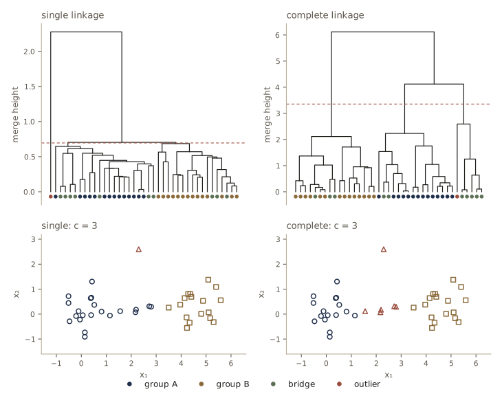
Stepwise-optimal hierarchical clustering
The linkage rules above have a minimum-variance flavor, but none of them optimizes a stated criterion. A simple change fixes that: at each step, merge the pair of clusters whose merger changes the chosen criterion least. For complete linkage this is already true of the largest cluster diameter. For \(J_e\) we need the increase caused by merging \(\mathcal{D}_i\) and \(\mathcal{D}_j\). The merged mean is \(\mathbf{m} = (n_i\mathbf{m}_i + n_j\mathbf{m}_j)/(n_i + n_j)\), and the same bookkeeping as in the transfer rule gives
\[J_{ij} - J_i - J_j = n_i \lVert \mathbf{m}_i - \mathbf{m} \rVert^2 + n_j \lVert \mathbf{m}_j - \mathbf{m} \rVert^2 = \frac{n_i n_j}{n_i + n_j} \lVert \mathbf{m}_i - \mathbf{m}_j \rVert^2 .\]So the stepwise-optimal choice merges the pair with the smallest
\[d_e(\mathcal{D}_i, \mathcal{D}_j) = \sqrt{\frac{n_i n_j}{n_i + n_j}}\, \lVert \mathbf{m}_i - \mathbf{m}_j \rVert ,\]a centroid distance weighted by the cluster sizes. This is usually called Ward’s method. The weight is small when either cluster is small, so the method tends to absorb singletons and small clusters into large ones before merging two medium-sized clusters. Its final partitions need not minimize \(J_e\) globally, but they are good starting points for iterative optimization. Let us check that each Ward merge raises \(J_e\) by exactly \(d_e^2\).
M = merges_h["ward"]
n_h = len(X_h)
worst = 0.0
for c in range(n_h - 1, 1, -1):                        # compare consecutive levels
    before, after = cut_tree(M, n_h, c + 1), cut_tree(M, n_h, c)
    increase = J_e(X_h, after) - J_e(X_h, before)
    worst = max(worst, abs(increase - M[n_h - c - 1][2] ** 2))
print(f"max |increase in J_e - d_e^2| over all merges: {worst:.1e}")
lab_w = cut_tree(M, n_h, 2)
print(f"Ward, c = 2: J_e = {J_e(X_h, lab_w):.3f}; after iterative transfers:"
      f" {J_e(X_h, transfer_pass(X_h, lab_w, rngt)[0]):.3f}")
max |increase in J_e - d_e^2| over all merges: 7.1e-15
first transfer: predicted change -1.2509, actual -1.2509
Ward, c = 2: J_e = 44.818; after iterative transfers: 42.120
Each merge raises \(J_e\) by exactly \(d_e^2\). The last two lines apply the transfer procedure of the previous section to Ward’s two-cluster partition (the middle line is its check of the first transfer): a few transfers lower \(J_e\) from 44.8 to 42.1, a reminder that a stepwise-optimal hierarchy gives good partitions, not optimal ones.
Hierarchical clustering and induced metrics
Agglomerative clustering needs only a dissimilarity \(\delta(\mathbf{x}, \mathbf{x}')\) between samples, not coordinates. With \(\delta_{\min}\) or \(\delta_{\max}\) between clusters, the merge order depends only on the ranking of the dissimilarities, so any monotonically increasing transformation of \(\delta\) (squaring it, say) gives the same dendrogram shape, with relabeled heights.
A dendrogram also defines a new distance: let \(d_c(\mathbf{x}, \mathbf{x}')\) be the height of the lowest merge at which \(\mathbf{x}\) and \(\mathbf{x}'\) fall into the same cluster (the cophenetic distance). It is nonnegative, symmetric, zero only for \(\mathbf{x} = \mathbf{x}'\), and when merge heights never decrease it satisfies a condition stronger than the triangle inequality,
\[d_c(\mathbf{x}, \mathbf{x}'') \le \max\left[d_c(\mathbf{x}, \mathbf{x}'),\, d_c(\mathbf{x}', \mathbf{x}'')\right] \quad \text{for every } \mathbf{x}',\]which makes it an ultrametric. The reason: whichever of the two merges joining \(\mathbf{x}'\) to \(\mathbf{x}\) and to \(\mathbf{x}''\) happens later has already put all three in one cluster. The cell checks the monotone-transformation claim, checks the ultrametric inequality on every triple, and computes the cophenetic correlation, the correlation between the cophenetic and the original distances, a common summary of how faithfully a dendrogram represents the data.
def cophenetic(merges, n):
    C = np.zeros((n, n))
    members = {i: [i] for i in range(n)}
    for t, (a, b, h, _) in enumerate(merges):
        ia, ib = members.pop(a), members.pop(b)
        C[np.ix_(ia, ib)] = h
        C[np.ix_(ib, ia)] = h
        members[n + t] = ia + ib
    return C

D_h = pdist(X_h)
iu = np.triu_indices(n_h, k=1)
for L in ["single", "complete", "average"]:
    same_order = [m[:2] for m in agglomerate(X_h, L, D_h ** 2)] == [m[:2] for m in merges_h[L]]
    C = cophenetic(merges_h[L], n_h)
    bound = np.maximum(C[:, :, None], C[None, :, :]).min(axis=1)   # min over x' of max(C[x,x'], C[x',x''])
    violations = int(np.sum(C > bound + 1e-12))
    r = np.corrcoef(C[iu], D_h[iu])[0, 1]
    print(f"{L:8s} same merges if squared: {same_order!s:5s}  ultrametric violations: {violations}"
          f"  cophenetic corr. {r:.3f}")

tri = np.array([[0.0, 0.0], [1.0, 0.0], [0.5, 0.9]])     # a centroid-linkage inversion
print("centroid linkage merge heights on three points:", [round(float(m[2]), 3) for m in agglomerate(tri, "centroid")])
single   same merges if squared: True   ultrametric violations: 0  cophenetic corr. 0.290
complete same merges if squared: True   ultrametric violations: 0  cophenetic corr. 0.842
average  same merges if squared: False  ultrametric violations: 0  cophenetic corr. 0.856
centroid linkage merge heights on three points: [1.0, 0.9]
For single and complete linkage the merge order is unchanged when the distances are squared (average linkage need not be, since averaging does not commute with squaring), and their cophenetic distances satisfy the ultrametric inequality on every triple. Centroid linkage can produce an inversion: in the three-point example the first two points merge at height 1, and the centroid of that pair is only 0.9 from the third point, so the second merge happens lower than the first. With inversions the dendrogram cannot be drawn with monotone heights and the cophenetic distance is not an ultrametric, which is one reason to prefer the other linkages. (On the bridge data, centroid linkage happens to produce no inversion.)
The problem of validity
Almost everything so far assumed the number of clusters \(c\) was known. Sometimes it is, for example when an existing classifier is being tuned. When we are exploring unknown data, deciding how many clusters are really there, the problem of cluster validity, is one of the hardest questions in the subject.
The usual informal approach is to cluster for \(c = 1, 2, 3, \dots\) and watch the criterion. \(J_e\) always decreases as \(c\) grows (at worst by moving one sample into a new singleton cluster) and is zero at \(c = n\), so the size of the decrease is what matters: with \(c^*\) compact, well-separated clusters, \(J_e\) should drop steeply up to \(c^*\) and slowly after. Large gaps between merge heights in a dendrogram make the same argument.
A more formal approach is a hypothesis test. Take as null hypothesis that exactly \(c\) clusters are present, find the sampling distribution of the criterion \(J(c + 1)\) under that hypothesis, and reject if the observed improvement is too large to be chance. Exact sampling distributions are out of reach, but DHS give a rough version for splitting one cluster. Suppose all \(n\) samples come from a single normal density with covariance \(\sigma^2\mathbf{I}\) in \(d\) dimensions. Then
- \(J_e(1) = \sum \lVert \mathbf{x} - \mathbf{m} \rVert^2\) is approximately normal with mean \(nd\sigma^2\) and variance \(2nd\sigma^4\);
- splitting by a hyperplane through the sample mean (a suboptimal but tractable partition) gives a \(J_e(2)\) that, for large \(n\), is approximately normal with mean \(n(d - 2/\pi)\sigma^2\) and variance \(2n(d - 8/\pi^2)\sigma^4\).
The mean follows from a short calculation: each half of a standard normal coordinate has mean \(\pm\sigma\sqrt{2/\pi}\), so splitting removes \(n(2/\pi)\sigma^2\) from the squared error along the normal of the hyperplane and nothing along the other \(d - 1\) directions. Estimating \(\sigma^2\) by \(J_e(1)/(nd)\) and treating the hyperplane split as nearly optimal gives the test: reject the one-cluster hypothesis at significance level \(p\) percent if
\[\frac{J_e(2)}{J_e(1)} < 1 - \frac{2}{\pi d} - \alpha\sqrt{\frac{2\,(1 - 8/(\pi^2 d))}{nd}}, \qquad p = 100\int_{\alpha}^{\infty} \frac{1}{\sqrt{2\pi}} e^{-u^2/2}\, du = 50\left(1 - \operatorname{erf}(\alpha/\sqrt{2})\right).\]A \(c\)-cluster solution can be examined by applying the test to each cluster. Let us check the two approximations by simulation and then see how the test behaves.
rngv = np.random.default_rng(1020)
n_v, d_v = 100, 2
J1s, J2s = [], []
for rep in range(2000):
    Xn = rngv.normal(size=(n_v, d_v))                  # null hypothesis, sigma = 1
    J1s.append(J_e(Xn, np.zeros(n_v, int)))
    J2s.append(J_e(Xn, (Xn[:, 0] > Xn[:, 0].mean()).astype(int)))   # fixed hyperplane through the mean
J1s, J2s = np.array(J1s), np.array(J2s)
print(f"J_e(1): mean {J1s.mean():7.2f} (theory {n_v * d_v}),  var {J1s.var():7.1f} (theory {2 * n_v * d_v})")
print(f"J_e(2): mean {J2s.mean():7.2f} (theory {n_v * (d_v - 2 / np.pi):.2f}),"
      f"  var {J2s.var():7.1f} (theory {2 * n_v * (d_v - 8 / np.pi ** 2):.1f})")

def split_test(X, rng, p=5.0):
    n, d = X.shape
    alpha = np.sqrt(2) * erfinv(1 - p / 50)             # solves p = 50 (1 - erf(alpha / sqrt 2))
    crit = 1 - 2 / (np.pi * d) - alpha * np.sqrt(2 * (1 - 8 / (np.pi ** 2 * d)) / (n * d))
    ratio = kmeans_best(X, 2, rng, restarts=3)[0] / J_e(X, np.zeros(n, int))
    return ratio, crit

ratios = np.array([split_test(rngv.normal(size=(n_v, d_v)), rngv)[0] for _ in range(300)])
crit = split_test(rngv.normal(size=(n_v, d_v)), rngv)[1]
print(f"alpha = {np.sqrt(2) * erfinv(0.9):.3f}, critical ratio {crit:.3f}")
print(f"null data, best 2-means split: ratio mean {ratios.mean():.3f}, sd {ratios.std():.3f},"
      f" rejected {np.mean(ratios < crit):.1%} of 300 (nominal 5%)")
print("three-group data X: ratio %.3f -> reject: %s" % (split_test(X, rngv)[0], split_test(X, rngv)[0] < crit))
J_e(1): mean  197.72 (theory 200),  var   421.0 (theory 400)
J_e(2): mean  133.16 (theory 136.34),  var   242.9 (theory 237.9)
alpha = 1.645, critical ratio 0.555
null data, best 2-means split: ratio mean 0.631, sd 0.024, rejected 0.7% of 300 (nominal 5%)
three-group data X: ratio 0.506 -> reject: True
The large-sample formulas for the means and variances hold up well. The test itself is rough, in both directions. The best 2-means split does better than a hyperplane through the mean in a fixed direction, which pushes the ratio down and would make the test reject too often; but the ratio \(J_e(2)/J_e(1)\) varies much less than the formula assumes, because \(J_e(1)\) and \(J_e(2)\) rise and fall together. Here the second effect wins and the test rejects less than 1 percent of the time at a nominal 5 percent: it is conservative. On the three-group data the ratio is far below the critical value and the split is clearly justified.
Watch out. Tests like this one rest on strong assumptions (a single spherical normal under the null, a nearly optimal split) and crude approximations, and the question of cluster validity is still essentially open. When the test matters, it is safer to calibrate it by simulation, as we just did: generate many data sets under the null hypothesis, cluster each one exactly as the real data were clustered, and compare.
Online clustering
All the procedures above optimize a global criterion over the whole data set with a fixed \(c\). Two practical problems follow. Every sample influences every cluster center, so new data can reorganize clusters that have nothing to do with it; and with a stream of data a system must be able to create clusters when something new appears. A system that adapts readily (it is plastic) tends to be unstable, and one whose clusters are stable tends to stop learning. This tension is called the stability–plasticity dilemma.
Competitive learning limits each update to the single cluster most similar to the current sample. DHS present it as a network with one output unit per cluster: each sample is augmented with \(x_0 = 1\) and scaled to unit length, each unit’s weight vector \(\mathbf{w}_j\) is kept at unit length, the unit with the largest activation \(\mathbf{w}_j^{t}\mathbf{x}\) wins, and only the winner learns: \(\mathbf{w}_j \leftarrow \mathbf{w}_j + \eta\,\mathbf{x}\), then \(\mathbf{w}_j \leftarrow \mathbf{w}_j/\lVert \mathbf{w}_j \rVert\). The normalization makes the competition depend only on angles (without it one unit’s weights could grow until it won every competition). Compared with decision-directed k-means, where each center is the mean of its current members, the update touches only one center, so distant clusters are left undisturbed; the price is that no global criterion is being minimized, and with a constant \(\eta\) the centers need never settle. A learning rate that decays over time makes them settle, but then the system can no longer learn a genuinely new pattern.
Unknown number of clusters
If \(c\) is unknown we can either solve the problem for many values of \(c\) and compare, as in the validity section, or set a threshold for creating a new cluster. The threshold approach suits on-line data. In leader–follower clustering, the first sample becomes the first cluster center. Each later sample finds its nearest center; if that center is closer than a threshold \(\theta\), the center (the leader) moves a little toward the sample (the follower), otherwise the sample founds a new cluster. DHS state the rule with the normalized weights of competitive learning; our version works with raw coordinates and moves the center a fraction \(\eta\) of the way toward the sample.
def leader_follower(X, theta, eta, order):
    W = [X[order[0]].copy()]
    for k in order[1:]:
        dist = np.linalg.norm(np.array(W) - X[k], axis=1)
        j = int(dist.argmin())
        if dist[j] < theta:
            W[j] += eta * (X[k] - W[j])                 # nearest center follows the sample
        else:
            W.append(X[k].copy())                       # the sample becomes a new leader
    return np.array(W)

rngl = np.random.default_rng(1011)
for theta in [1.5, 2.5, 3.5, 5.0]:
    counts = [len(leader_follower(X, theta, 0.1, np.tile(rngl.permutation(len(X)), 3))) for _ in range(5)]
    print(f"theta = {theta}: number of clusters in 5 random presentation orders {counts}")
theta = 1.5: number of clusters in 5 random presentation orders [11, 12, 11, 12, 10]
theta = 2.5: number of clusters in 5 random presentation orders [5, 4, 5, 5, 5]
theta = 3.5: number of clusters in 5 random presentation orders [3, 3, 3, 3, 3]
theta = 5.0: number of clusters in 5 random presentation orders [2, 2, 3, 2, 2]
The threshold implicitly sets the number of clusters: a small \(\theta\) gives many small clusters, a large one a few large ones, and near the boundary between two regimes the answer depends on the order in which the samples arrive. There is no principled rule for \(\theta\) without knowing something about the data, and the basic algorithm never merges clusters that turn out to be close.
Adaptive resonance
Adaptive resonance theory (ART) is a family of neural network models built around leader–follower clustering and aimed at the stability–plasticity dilemma. Cluster units are connected to the input layer by bottom-up weights (the cluster centers, as in competitive learning) and top-down weights (the pattern each cluster expects to see). When a sample arrives, the most active cluster unit sends its expectation back down; if input and expectation agree, the network settles into a stable state (the “resonance”) and the winning center moves slightly toward the sample. If they disagree by more than a user-chosen vigilance \(\rho\), the winner is suppressed and the search continues, and if no cluster matches, a new cluster unit is recruited. Vigilance plays the role of the threshold \(\theta\): low vigilance gives a few coarse clusters, high vigilance many fine ones. Because a cluster only absorbs samples that match it well, old clusters are protected from being overwritten by new, different data. DHS §10.11.2 gives the outline; a working network needs many more details.
Learning with a critic
Between supervised learning (a teacher gives the category) and unsupervised learning (nobody says anything) lies learning with a critic: after the system assigns a sample to a cluster or category, a critic says only whether the assignment was right or wrong. This is easy to add to competitive learning or ART: when the critic approves, the usual update is made; when it disapproves, the update is withheld (or, in some variants, the winning center is moved away from the sample). The idea connects to reinforcement learning, where feedback is a reward rather than a label.
Graph-theoretic methods
Normal mixtures and minimum-variance criteria picture clusters as isolated compact clumps. Graph theory lets us describe more intricate structures, such as chains, rings, or dense cores in sparse surroundings. There is no single way to cast clustering as a graph problem, and using these ideas well takes some creativity.
Pick a similarity \(s\) and a threshold \(s_0\) (or a distance and a threshold \(d_0\)), and define the \(n \times n\) similarity matrix with entries 1 when two samples are similar enough and 0 otherwise. It is the adjacency matrix of a similarity graph whose nodes are the samples. Our first clustering rule, joining samples closer than \(d_0\), took the connected components of this graph, and that is exactly single linkage stopped at height \(d_0\): two samples share a cluster when a chain of similar pairs joins them. Complete linkage asks instead that all pairs within a cluster be similar, which corresponds to maximal complete subgraphs (cliques) of the graph; since cliques can overlap, the complete-linkage clusters are found among them but cannot be read off the thresholded graph alone.
The minimal spanning tree. A spanning tree connects all \(n\) samples with \(n - 1\) edges and no loops; a minimal spanning tree (MST) has the smallest total edge length. Single linkage run to the end builds exactly an MST: each merge adds the shortest edge joining two different clusters, which is Kruskal’s algorithm, so the \(n - 1\) single-linkage merge heights are the MST’s edge lengths. Conversely, from the MST we can recover every single-linkage clustering: removing the longest edge leaves two components, the two-cluster single-linkage solution; removing the next longest gives three; and so on. This is a divisive hierarchical procedure.
To build the MST we use Prim’s algorithm, which grows one tree from an arbitrary starting sample: keep, for every sample outside the tree, its distance to the nearest sample inside, and repeatedly add the outside sample with the smallest such distance. On the complete graph of \(n\) samples this costs \(O(n^2)\) with plain arrays.
def prim_mst(X):
    """Minimal spanning tree of the complete Euclidean graph. Returns edges (i, j, length)."""
    n = len(X)
    D = pdist(X)
    in_tree = np.zeros(n, bool)
    in_tree[0] = True
    best = D[0].copy()                 # distance from each sample to the tree
    link = np.zeros(n, int)            # the tree sample that achieves it
    edges = []
    for _ in range(n - 1):
        j = int(np.where(in_tree, np.inf, best).argmin())
        edges.append((int(link[j]), j, float(best[j])))
        in_tree[j] = True
        closer = D[j] < best
        best[closer], link[closer] = D[j][closer], j
    return edges

mst_h = prim_mst(X_h)
print("MST edge lengths equal the single-linkage merge heights:",
      np.allclose(np.sort([e[2] for e in mst_h]), np.sort([m[2] for m in merges_h["single"]])))

rngm = np.random.default_rng(1013)
X_m = np.vstack([rngm.normal([0, 0], 0.25, (25, 2)),        # dense
                 rngm.normal([3, 0.3], 0.5, (25, 2)),       # medium
                 rngm.normal([1.2, 3.2], 0.9, (25, 2))])    # sparse
group_m = np.repeat(np.arange(3), 25)
mst = prim_mst(X_m)
lengths = np.array([e[2] for e in mst])
print(f"MST of 75 samples: total length {lengths.sum():.3f}, five longest edges {np.sort(lengths)[-5:].round(2)}")
for k in [2, 3, 4]:
    keep = [e[:2] for e in mst if e[2] < np.sort(lengths)[-(k - 1)]]      # remove the k-1 longest edges
    lab = connected_components(len(X_m), keep)
    groups_in = [np.bincount(group_m[lab == i], minlength=3).tolist() for i in range(lab.max() + 1)]
    print(f"remove {k - 1} longest: sizes {np.bincount(lab).tolist()}, groups {groups_in}")
MST edge lengths equal the single-linkage merge heights: True
MST of 75 samples: total length 21.726, five longest edges [0.74 0.91 1.02 1.7  1.77]
remove 1 longest: sizes [25, 50], groups [[0, 25, 0], [25, 0, 25]]
remove 2 longest: sizes [25, 25, 25], groups [[25, 0, 0], [0, 25, 0], [0, 0, 25]]
remove 3 longest: sizes [25, 25, 24, 1], groups [[25, 0, 0], [0, 25, 0], [0, 0, 24], [0, 0, 1]]
Removing the two longest edges recovers the three groups exactly. Removing a third does not find a fourth group; it splits one sample off the sparse group, whose internal edges are longer than any edge inside the dense group. A global length threshold cannot serve groups of different densities at once.
A more local rule compares each edge with its neighbors. Call an edge inconsistent if its length is much larger, say more than twice, than the average length of the other edges that touch its two end points, and remove all inconsistent edges. The rule adapts to local density, since a long edge in a sparse region is compared with other long edges.
touching = {i: [] for i in range(len(X_m))}
for k, (i, j, _) in enumerate(mst):
    touching[i].append(k)
    touching[j].append(k)
ratio = np.array([l / np.mean([mst[m][2] for m in set(touching[i] + touching[j]) if m != k])
                  if len(set(touching[i] + touching[j])) > 1 else 0.0
                  for k, (i, j, l) in enumerate(mst)])
for thr in [2.0, 3.0]:
    keep = [e[:2] for k, e in enumerate(mst) if ratio[k] <= thr]
    lab = connected_components(len(X_m), keep)
    sizes_r = np.sort(np.bincount(lab))[::-1].tolist()
    print(f"remove edges with ratio > {thr}: {int(np.sum(ratio > thr))} edges, cluster sizes {sizes_r}")
remove edges with ratio > 2.0: 11 edges, cluster sizes [23, 16, 9, 9, 6, 4, 3, 1, 1, 1, 1, 1]
remove edges with ratio > 3.0: 3 edges, cluster sizes [25, 25, 24, 1]
With 75 samples the local averages are noisy: a threshold of 2 cuts eleven edges and fragments the groups, while a threshold of 3 finds the three groups and cuts off one extra sample. Local rules need more data, or more careful definitions of the neighborhood (for example, averaging over edges within two steps of each end), to be reliable.
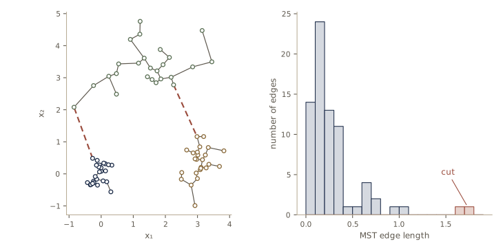
The MST supports other descriptive statistics too. Its edge-length distribution can separate dense clusters from a sparse background (delete the long edges and the dense clusters remain as large components). The diameter path, the longest path in the tree, is a natural skeleton for chain-shaped data: a chain has few and short branches off its diameter path, while a round cloud has many. And while a small move of one sample can reroute an MST, such summary statistics change little.
Component analysis
Clustering groups the samples. Component analysis looks for good features instead: new variables, computed from the data without labels, that capture its structure. DHS discuss three methods with different goals.
Principal component analysis
Module 03 introduced principal component analysis (PCA), also called the Karhunen–Loève transform, and Intro to ML, module 12 derives it from both the maximum-variance and the minimum-error points of view. In brief: compute the sample mean \(\boldsymbol{\mu}\) and covariance \(\boldsymbol{\Sigma}\) of all the data, find the eigenvectors \(\mathbf{e}_1, \mathbf{e}_2, \dots\) of \(\boldsymbol{\Sigma}\) sorted by decreasing eigenvalue \(\lambda_1 \ge \lambda_2 \ge \cdots\), collect the first \(k\) as the columns of a \(d \times k\) matrix \(\mathbf{A}\), and represent each sample by
\[\mathbf{y} = \mathbf{A}^{t}(\mathbf{x} - \boldsymbol{\mu}).\]Among all \(k\)-dimensional linear subspaces this one minimizes the mean squared distance between the samples and their projections, and that minimum equals the sum of the discarded eigenvalues \(\lambda_{k+1} + \cdots + \lambda_d\). A few large eigenvalues followed by many small ones suggest that the data effectively live in \(k\) dimensions, with the rest being noise.
A neural-network view connects PCA to what follows. Train a network with \(d\) inputs, \(k\) linear hidden units and \(d\) linear outputs to reproduce its input at its output (an autoencoder), by gradient descent on the squared reconstruction error. At the minimum the hidden units span the same subspace as the first \(k\) principal components (the individual hidden units need not be the eigenvectors themselves; any basis of the subspace does equally well).
rngp = np.random.default_rng(1013)
Q4 = np.linalg.qr(rngp.normal(size=(4, 4)))[0]                   # a random rotation of R^4
X_p = np.column_stack([rngp.normal(size=(200, 2)) * [2.0, 1.0],
                       0.2 * rngp.normal(size=(200, 2))]) @ Q4.T + [1.0, -2.0, 0.5, 3.0]
Xc_p = X_p - X_p.mean(axis=0)
lam_p, E_p = np.linalg.eigh(Xc_p.T @ Xc_p / len(X_p))
lam_p, E_p = lam_p[::-1], E_p[:, ::-1]
A_pca = E_p[:, :2]
err_pca = ((Xc_p - Xc_p @ A_pca @ A_pca.T) ** 2).sum(axis=1).mean()
print(f"eigenvalues {lam_p};  PCA error (k = 2) {err_pca:.5f} = sum of the last two {lam_p[2:].sum():.5f}")

W_in, W_out = 0.1 * rngp.normal(size=(2, 4)), 0.1 * rngp.normal(size=(4, 2))   # d-k-d linear autoencoder
for step in range(3000):
    H = Xc_p @ W_in.T                                  # hidden units
    E_rec = H @ W_out.T - Xc_p                         # reconstruction error
    g_out = 2 * E_rec.T @ H / len(Xc_p)
    g_in = 2 * (E_rec @ W_out).T @ Xc_p / len(Xc_p)
    W_out -= 0.02 * g_out
    W_in -= 0.02 * g_in
err_ae = ((Xc_p @ W_in.T @ W_out.T - Xc_p) ** 2).sum(axis=1).mean()
cosines = np.linalg.svd(A_pca.T @ np.linalg.qr(W_out)[0], compute_uv=False)
print(f"autoencoder error {err_ae:.5f}; cosines of the angles between its subspace and PCA's: {cosines}")
eigenvalues [3.9715 1.1218 0.0426 0.0332];  PCA error (k = 2) 0.07578 = sum of the last two 0.07578
autoencoder error 0.07578; cosines of the angles between its subspace and PCA's: [1. 1.]
Nonlinear component analysis
If the data lie near a curved surface, no linear subspace represents them well. Nonlinear component analysis (NLCA) replaces the linear autoencoder by one with five layers: \(d\) inputs, a layer of nonlinear (for example \(\tanh\)) units, a bottleneck of \(k\) linear units, another nonlinear layer, and \(d\) linear outputs. The first half learns a nonlinear projection \(F_1\) from the data to \(k\) numbers, the second half a nonlinear map \(F_2\) back to \(d\) dimensions, and training on reconstruction error with backpropagation (module 06) makes the image of \(F_2\) a \(k\)-dimensional curved surface through the data. After training, the bottleneck outputs are the nonlinear components. Both nonlinear layers are needed: without them the network can only represent a linear subspace.
Here is a small example: 150 noisy points on an arc of a circle, reduced to one component. We train a \(2\)–\(12\)–\(1\)–\(12\)–\(2\) network with full-batch gradient descent using the Adam step rule (a gradient method that adapts the step size per weight; any careful gradient method would do). The backpropagation code follows module 06; a finite-difference check of its gradient agrees to eight digits, which we omit here.
rnga = np.random.default_rng(1014)
ang = rnga.uniform(0.1 * np.pi, 0.9 * np.pi, 150)
X_arc = 2 * np.column_stack([np.cos(ang), np.sin(ang)]) + 0.08 * rnga.normal(size=(150, 2))
X_arc -= X_arc.mean(axis=0)
e1 = np.linalg.eigh(X_arc.T @ X_arc)[1][:, -1]
print(f"PCA with one component: mean squared error {((X_arc - np.outer(X_arc @ e1, e1)) ** 2).sum(1).mean():.4f}")

sizes_ae, acts = [2, 12, 1, 12, 2], ["tanh", "linear", "tanh", "linear"]
params = []
for a, b in zip(sizes_ae[:-1], sizes_ae[1:]):
    params += [rnga.normal(size=(a, b)) / np.sqrt(a), np.zeros(b)]      # W, b per layer

def ae_forward(params, X):
    hs = [X]
    for l, act in enumerate(acts):
        z = hs[-1] @ params[2 * l] + params[2 * l + 1]
        hs.append(np.tanh(z) if act == "tanh" else z)
    return hs

def ae_loss_grads(params, X):
    hs = ae_forward(params, X)
    delta = 2 * (hs[-1] - X) / len(X)                 # derivative of the mean squared error
    grads = [None] * len(params)
    for l in range(len(acts) - 1, -1, -1):
        grads[2 * l], grads[2 * l + 1] = hs[l].T @ delta, delta.sum(axis=0)
        if l > 0:
            delta = delta @ params[2 * l].T
            if acts[l - 1] == "tanh":
                delta = delta * (1 - hs[l] ** 2)
    return ((hs[-1] - X) ** 2).sum(axis=1).mean(), grads

m_adam = [np.zeros_like(p) for p in params]
v_adam = [np.zeros_like(p) for p in params]
for t in range(1, 4001):
    loss, grads = ae_loss_grads(params, X_arc)
    for i, g in enumerate(grads):
        m_adam[i] = 0.9 * m_adam[i] + 0.1 * g
        v_adam[i] = 0.999 * v_adam[i] + 0.001 * g ** 2
        params[i] -= 0.01 * (m_adam[i] / (1 - 0.9 ** t)) / (np.sqrt(v_adam[i] / (1 - 0.999 ** t)) + 1e-8)
    if t in [1, 500, 2000, 4000]:
        print(f"step {t:4d}: reconstruction error {loss:.4f}")
code = ae_forward(params, X_arc)[2][:, 0]              # the bottleneck output
print(f"correlation between the nonlinear component and the angle along the arc: {np.corrcoef(code, ang)[0, 1]:.4f}")
PCA with one component: mean squared error 0.1730
step    1: reconstruction error 1.7368
step  500: reconstruction error 0.0065
step 2000: reconstruction error 0.0056
step 4000: reconstruction error 0.0055
correlation between the nonlinear component and the angle along the arc: 0.9948
One linear component can only project the arc onto a line and loses its curvature; one nonlinear component reconstructs the arc with an error more than twenty times smaller, and the bottleneck unit has learned, up to sign and a monotone distortion, the position along the arc. The costs are those of neural networks in general: a nonconvex error surface with local minima, and a bottleneck size \(k\) to choose (train for several \(k\) and look for the point where the error stops improving much, as with the eigenvalue spectrum in PCA).
Watch out. Components that represent the data well need not help to classify it. If the classes differ along a direction of small variance while noise dominates another direction, the leading linear or nonlinear component captures the noise and throws the class information away. For classification, directions chosen with the labels, such as Fisher’s multiple discriminant analysis, are the right tool.
Independent component analysis
Independent component analysis (ICA) seeks directions that make the resulting components as statistically independent as possible, rather than as good at reconstruction as possible. Its natural home is blind source separation. Let \(d\) independent source signals \(x_1(t), \dots, x_d(t)\) (DHS use \(\mathbf{x}\) for the sources and \(\mathbf{s}\) for the sensors, and we follow them here) have zero mean and joint density \(p(\mathbf{x}) = \prod_i p(x_i)\). We observe only linear mixtures of them at \(d\) sensors,
\[\mathbf{s}(t) = \mathbf{A}\,\mathbf{x}(t),\]for example the signals of \(d\) microphones picking up \(d\) speakers, ignoring delays and echoes. Neither \(\mathbf{A}\) nor the sources are known. The goal is a matrix \(\mathbf{W}\) such that the components of \(\mathbf{W}\mathbf{s}\) are independent; if the model holds, they are then the sources, up to order and scale.
The approach in DHS (the “infomax” principle of Bell and Sejnowski) passes the unmixed signals through a squashing function, \(\mathbf{y} = f(\mathbf{u})\) with \(\mathbf{u} = \mathbf{W}\mathbf{s} + \mathbf{w}_0\) and \(f\) the logistic sigmoid applied to each component, and maximizes the joint entropy of the outputs,
\[H(\mathbf{y}) = -\mathcal{E}\left[\ln p_{\mathbf{y}}(\mathbf{y})\right] = \mathcal{E}\left[\ln \lvert \mathbf{J} \rvert\right] - \mathcal{E}\left[\ln p_{\mathbf{s}}(\mathbf{s})\right],\]where \(\mathcal{E}\) is an average over the samples \(t = 1, \dots, T\) and \(\mathbf{J}\) is the Jacobian matrix of the map from \(\mathbf{s}\) to \(\mathbf{y}\) (so \(p_{\mathbf{y}} = p_{\mathbf{s}}/\lvert \mathbf{J} \rvert\)). The second term does not depend on the weights. For \(\mathbf{y} = f(\mathbf{W}\mathbf{s} + \mathbf{w}_0)\) the Jacobian is \(\operatorname{diag}(f'(u_i))\,\mathbf{W}\), so
\[\ln \lvert \mathbf{J} \rvert = \ln \lvert \mathbf{W} \rvert + \sum_{i=1}^{d} \ln f'(u_i).\]The derivative of \(\ln \lvert \mathbf{W} \rvert\) with respect to \(\mathbf{W}\) is \([\mathbf{W}^{t}]^{-1}\) (each entry is a cofactor divided by the determinant). For the logistic function \(f' = y(1 - y)\), so \(\frac{d}{du}\ln f'(u) = 1 - 2y\). Gradient ascent on \(H\) therefore uses
\[\Delta\mathbf{W} \propto [\mathbf{W}^{t}]^{-1} + \mathcal{E}\left[(\mathbf{1} - 2\mathbf{y})\,\mathbf{s}^{t}\right], \qquad \Delta\mathbf{w}_0 \propto \mathcal{E}\left[\mathbf{1} - 2\mathbf{y}\right],\]with \(\mathbf{1}\) a vector of ones. A widely used improvement multiplies the gradient on the right by \(\mathbf{W}^{t}\mathbf{W}\) (the natural gradient, which accounts for the geometry of the space of matrices). Using \(\mathbf{u} = \mathbf{W}\mathbf{s}\) for centered data, this gives
\[\Delta\mathbf{W} \propto \left(\mathbf{I} + \mathcal{E}\left[(\mathbf{1} - 2\mathbf{y})\,\mathbf{u}^{t}\right]\right)\mathbf{W},\]which needs no matrix inverse and converges much faster. Two practical points. First, whitening the sensor signals (making their covariance the identity) before ICA removes all second-order dependence, so ICA only has to find a rotation; PCA alone cannot find it, because rotated white data are still white. Second, the logistic nonlinearity suits sources with heavier tails than a Gaussian (positive excess kurtosis), such as speech; sources with lighter tails need a different nonlinearity, and Gaussian sources cannot be separated at all, since any rotation of independent Gaussians is again independent Gaussians.
Our sources are a bursty oscillation, on for a while and off for a while, and heavy-tailed Laplace noise, 2000 samples each, mixed by a matrix that we then pretend not to know.
rngi = np.random.default_rng(1016)
T_ica = 2000
t_ica = np.arange(T_ica)
bursts = (np.sin(2 * np.pi * t_ica / 400) > 0.3) * np.sin(2 * np.pi * t_ica / 23)
src = np.vstack([bursts, rngi.laplace(size=T_ica)])
src = (src - src.mean(axis=1, keepdims=True)) / src.std(axis=1, keepdims=True)   # sources x(t), shape (d, T)
def excess_kurtosis(v):
    v = (v - v.mean()) / v.std()
    return (v ** 4).mean() - 3
print(f"excess kurtosis of the sources: {excess_kurtosis(src[0]):.2f}, {excess_kurtosis(src[1]):.2f}")

A_mix = np.array([[1.0, 1.0], [0.2, 1.0]])
sens = A_mix @ src                                     # sensor signals s(t) = A x(t)
sens_c = sens - sens.mean(axis=1, keepdims=True)
lam_s, E_s = np.linalg.eigh(sens_c @ sens_c.T / T_ica)
V_white = E_s @ np.diag(lam_s ** -0.5) @ E_s.T         # symmetric whitening matrix
Z_w = V_white @ sens_c

def infomax_natural(Z, eta=0.1, iters=300):
    d, T = Z.shape
    W = np.eye(d)
    for it in range(iters):
        U = W @ Z
        Y = expit(U)
        dW = (np.eye(d) + (1 - 2 * Y) @ U.T / T) @ W   # natural-gradient ascent on H(y)
        W += eta * dW
        if it in (0, 49, iters - 1):
            print(f"  iteration {it + 1:3d}: largest update entry {np.abs(dW).max():.2e}")
    return W

def infomax_plain(Z, eta=0.05, iters=3000):
    W = np.eye(Z.shape[0])
    for _ in range(iters):
        Y = expit(W @ Z)
        W += eta * (np.linalg.inv(W).T + (1 - 2 * Y) @ Z.T / Z.shape[1])   # the gradient as derived above
    return W

def corr_with_sources(Y):
    return np.corrcoef(np.vstack([Y, src]))[:2, 2:]

print(f"sample correlation of the two sources themselves: {np.corrcoef(src)[0, 1]:.4f}")
print("whitened sensors vs sources:\n", corr_with_sources(Z_w))
W_ica = infomax_natural(Z_w)
print("natural-gradient ICA outputs vs sources:\n", corr_with_sources(W_ica @ Z_w))
print("plain-gradient ICA (3000 iterations) outputs vs sources:\n", corr_with_sources(infomax_plain(Z_w) @ Z_w))
excess kurtosis of the sources: 0.73, 2.72
sample correlation of the two sources themselves: -0.0319
whitened sensors vs sources:
 [[ 0.9211  0.3596]
 [-0.3892  0.9331]]
  iteration   1: largest update entry 6.15e-01
  iteration  50: largest update entry 9.15e-02
  iteration 300: largest update entry 1.35e-05
natural-gradient ICA outputs vs sources:
 [[ 1.     -0.0267]
 [-0.0142  0.9998]]
plain-gradient ICA (3000 iterations) outputs vs sources:
 [[ 1.     -0.0267]
 [-0.0142  0.9998]]
Each row of these tables correlates one signal with the two true sources. Whitening decorrelates the sensors but leaves each of its outputs mixing both sources (correlations of about 0.9 and 0.4). After ICA each output matches one source with correlation 0.9998 or better in absolute value, and its correlation with the other source, about 0.02, is no larger than the sample correlation between the two sources themselves. The plain gradient of the DHS derivation reaches the same answer here too; we gave it 3000 iterations, each with a matrix inverse, against 300 for the natural gradient. The outputs come back in some order and with some sign and scale, which is all that blind separation can promise (Figure 6).
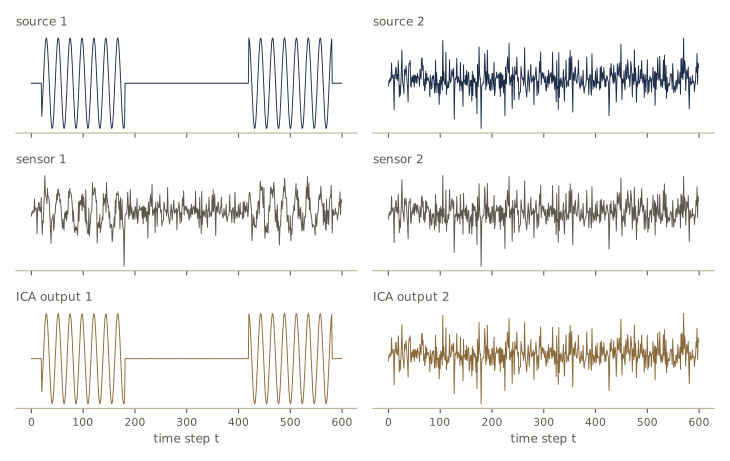
As preprocessing for classification, ICA has an advantage over PCA and NLCA when the features really are produced by independent processes: it extracts those processes instead of the directions of largest variance. How many components to extract is again a choice; with a known number of classes and no other information, DHS suggest starting with that many.
Multidimensional scaling and self-organizing maps
Part of what makes clustering hard to judge is that we cannot look at data in many dimensions, and some data come only as dissimilarities, with no coordinates at all. Multidimensional scaling (MDS) looks for points \(\mathbf{y}_1, \dots, \mathbf{y}_n\) in a low-dimensional space, usually two or three dimensions, whose distances \(d_{ij} = \lVert \mathbf{y}_i - \mathbf{y}_j \rVert\) match given dissimilarities \(\delta_{ij}\) as closely as possible.
Classical MDS
If the \(\delta_{ij}\) are Euclidean distances between points \(\mathbf{x}_i\), there is a closed-form answer. Let \(\boldsymbol{\Delta}^{(2)}\) be the matrix of squared dissimilarities and \(\mathbf{J} = \mathbf{I} - \frac{1}{n}\mathbf{1}\mathbf{1}^{t}\) the centering matrix. Expanding \(\delta_{ij}^2 = \lVert \mathbf{x}_i \rVert^2 + \lVert \mathbf{x}_j \rVert^2 - 2\mathbf{x}_i^{t}\mathbf{x}_j\) and centering rows and columns (double centering) cancels the squared-norm terms and leaves the matrix of inner products of the centered points,
\[\mathbf{B} = -\tfrac{1}{2}\,\mathbf{J}\,\boldsymbol{\Delta}^{(2)}\,\mathbf{J} = \mathbf{X}_c\mathbf{X}_c^{t}.\]\(\mathbf{B}\) is symmetric and positive semidefinite, so \(\mathbf{B} = \mathbf{V}\boldsymbol{\Lambda}\mathbf{V}^{t}\), and \(\mathbf{Y} = \mathbf{V}_k\boldsymbol{\Lambda}_k^{1/2}\) (the top \(k\) eigenvectors, scaled) reproduces the configuration exactly when \(k\) is at least its dimension, up to rotation and reflection. With fewer dimensions it gives the PCA projection of the points. If the dissimilarities are not Euclidean, \(\mathbf{B}\) has negative eigenvalues, and classical MDS gives only an approximation, usually a good starting point for the iterative method below.
def classical_mds(Delta, k):
    n = len(Delta)
    J = np.eye(n) - np.ones((n, n)) / n
    B = -0.5 * J @ (Delta ** 2) @ J                    # double centering
    lam, V = np.linalg.eigh(B)
    lam, V = lam[::-1], V[:, ::-1]
    return V[:, :k] * np.sqrt(np.maximum(lam[:k], 0)), lam

X8 = rngi.normal(size=(8, 3))                          # Euclidean distances of 8 points in 3-D
Y8, lam8 = classical_mds(pdist(X8), 3)
print(f"eigenvalues of B: {lam8.round(4)}")
print(f"largest error in the reproduced distances: {np.abs(pdist(Y8) - pdist(X8)).max():.1e}")
eigenvalues of B: [15.2638  2.0624  1.2431  0.      0.      0.     -0.     -0.    ]
largest error in the reproduced distances: 1.8e-15
Stress-based MDS
In general no configuration reproduces all the dissimilarities, and we minimize a criterion. Three natural sum-of-squared-error choices, sums running over pairs \(i < j\), are
\[J_{ee} = \frac{\sum_{i<j} (d_{ij} - \delta_{ij})^2}{\sum_{i<j} \delta_{ij}^2}, \qquad J_{ff} = \sum_{i<j} \left(\frac{d_{ij} - \delta_{ij}}{\delta_{ij}}\right)^2, \qquad J_{ef} = \frac{1}{\sum_{i<j} \delta_{ij}} \sum_{i<j} \frac{(d_{ij} - \delta_{ij})^2}{\delta_{ij}} .\]All depend only on distances, so they are unchanged by translating, rotating or reflecting the configuration, and they are normalized so that their minimum values do not change if all the dissimilarities are scaled. \(J_{ee}\) weighs large absolute errors most, \(J_{ff}\) large relative errors, and \(J_{ef}\), which weights each squared error by \(1/\delta_{ij}\), is a compromise that pays attention to preserving small distances, the local neighborhoods. Since \(\nabla_{\mathbf{y}_k} d_{kj}\) is the unit vector \((\mathbf{y}_k - \mathbf{y}_j)/d_{kj}\), the gradients are simple; for example
\[\nabla_{\mathbf{y}_k} J_{ef} = \frac{2}{\sum_{i<j} \delta_{ij}} \sum_{j \neq k} \frac{d_{kj} - \delta_{kj}}{\delta_{kj}} \, \frac{\mathbf{y}_k - \mathbf{y}_j}{d_{kj}} .\]We start from any configuration that spreads the points out (classical MDS, or the \(k\) coordinates of largest variance) and follow the negative gradient. Our test case has dissimilarities that no flat configuration can match: 40 points on a spherical cap reaching 70 degrees from the pole, with \(\delta_{ij}\) their great-circle distances along the surface. Flattening a curved surface must distort some distances, just as every flat map of the Earth does.
rngs2 = np.random.default_rng(1017)
colat = np.arccos(1 - rngs2.uniform(0, 1 - np.cos(np.radians(70)), 40))   # uniform on the cap
lon = rngs2.uniform(0, 2 * np.pi, 40)
P_sph = np.column_stack([np.sin(colat) * np.cos(lon), np.sin(colat) * np.sin(lon), np.cos(colat)])
Delta_g = np.arccos(np.clip(P_sph @ P_sph.T, -1, 1))                       # great-circle distances
iu40 = np.triu_indices(40, k=1)

def J_ef(Y, Delta):
    d, dl = pdist(Y)[iu40], Delta[iu40]
    return ((d - dl) ** 2 / dl).sum() / dl.sum()

def grad_J_ef(Y, Delta):
    dY, Dl = pdist(Y), Delta.copy()
    np.fill_diagonal(dY, 1.0)
    np.fill_diagonal(Dl, 1.0)
    coef = (dY - Dl) / (Dl * dY)
    np.fill_diagonal(coef, 0.0)
    return 2 / Delta[iu40].sum() * (coef[:, :, None] * (Y[:, None, :] - Y[None, :, :])).sum(axis=1)

Y_g, lam_g = classical_mds(Delta_g, 2)
print(f"eigenvalues of B: three largest {lam_g[:3].round(3)}, three smallest {lam_g[-3:].round(3)}")
G = grad_J_ef(Y_g, Delta_g)
E0 = np.zeros_like(Y_g)
E0[5, 1] = 1e-6
print(f"gradient check: {G[5, 1]:.6e} vs {(J_ef(Y_g + E0, Delta_g) - J_ef(Y_g - E0, Delta_g)) / 2e-6:.6e}")
print(f"classical MDS start: J_ef = {J_ef(Y_g, Delta_g):.5f}")
for step in range(1, 501):
    Y_g -= 0.1 * grad_J_ef(Y_g, Delta_g)
    if step in (50, 200, 500):
        print(f"after {step} gradient steps: J_ef = {J_ef(Y_g, Delta_g):.5f}")
eigenvalues of B: three largest [14.276  9.632  0.686], three smallest [-0.047 -0.939 -1.04 ]
gradient check: -1.239920e-03 vs -1.239920e-03
classical MDS start: J_ef = 0.00236
after 50 gradient steps: J_ef = 0.00178
after 200 gradient steps: J_ef = 0.00131
after 500 gradient steps: J_ef = 0.00122
The negative eigenvalues of \(\mathbf{B}\) confirm that the great-circle distances are not Euclidean. Classical MDS gives a reasonable disk-shaped starting map; gradient descent on \(J_{ef}\) rearranges it and roughly halves the criterion, but no flat configuration can bring it to zero.
Nonmetric MDS. Sometimes only the rank order of the dissimilarities is meaningful (a subject says which pairs of sounds are more alike, not by how much). Nonmetric MDS then asks only that the order of the \(d_{ij}\) match the order of the \(\delta_{ij}\). For a configuration, let \(\hat{d}_{ij}\) be the numbers closest (in squared error) to the \(d_{ij}\) among all numbers that are ordered like the \(\delta_{ij}\) (a monotone regression). The criterion \(\sum (d_{ij} - \hat{d}_{ij})^2\) measures how badly the configuration violates the order, and dividing by \(\sum d_{ij}^2\) stops the trivial solution of collapsing all points to one. Because the number of order constraints grows like \(n^2\) while the number of coordinates grows like \(n\), a good nonmetric solution pins the configuration down surprisingly well: metric structure is recovered from rank information alone.
Self-organizing feature maps
A self-organizing feature map (Kohonen map, topologically ordered map) also places the data in a low-dimensional target space so that neighbors stay neighbors, but it learns a mapping on-line without storing all pairwise dissimilarities. The target space is a set of units arranged on a line or a grid; unit \(k\) carries a weight vector \(\mathbf{w}_k\) in the source space. For each sample \(\mathbf{x}\), the winning unit \(k^*\) is the one whose weights are closest to \(\mathbf{x}\), and every unit is pulled toward \(\mathbf{x}\) in proportion to how near it is to the winner in the target space:
\[\mathbf{w}_k \leftarrow \mathbf{w}_k + \eta(t)\, \Lambda(\lvert k - k^* \rvert)\, (\mathbf{x} - \mathbf{w}_k).\]The window function \(\Lambda\) is 1 at the winner and decreases with distance on the grid; we use a Gaussian whose width shrinks during training, and a learning rate \(\eta(t)\) that decays so that learning eventually stops. (DHS state the rule with normalized weights and a dot-product winner, like competitive learning; we use unnormalized weights and Euclidean distance.) The window is what makes the map ordered: neighbors of the winner move in the same direction, so units adjacent on the line end up with nearby weights. We train a chain of 30 units on samples spread uniformly over a square, starting from a random tangle near the center, and count how many pairs of the chain’s segments cross each other.
def count_crossings(W):
    """Number of pairs of non-adjacent chain segments that intersect."""
    def orient(p, q, r):
        return np.sign((q[0] - p[0]) * (r[1] - p[1]) - (q[1] - p[1]) * (r[0] - p[0]))
    count = 0
    for i in range(len(W) - 1):
        for j in range(i + 2, len(W) - 1):
            a, b, c_, d_ = W[i], W[i + 1], W[j], W[j + 1]
            if orient(a, b, c_) != orient(a, b, d_) and orient(c_, d_, a) != orient(c_, d_, b):
                count += 1
    return count

def som_chain(W, X, steps, rng, eta0=0.5, eta1=0.01, width0=8.0, width1=0.5, snapshots=()):
    W = W.copy()
    pos = np.arange(len(W))
    saved = {0: W.copy()}
    for t in range(steps):
        x = X[rng.integers(len(X))]
        frac = t / steps
        eta = eta0 * (eta1 / eta0) ** frac                 # decaying learning rate
        width = width0 * (width1 / width0) ** frac         # shrinking window
        k_star = np.argmin(((W - x) ** 2).sum(axis=1))
        W += eta * np.exp(-0.5 * ((pos - k_star) / width) ** 2)[:, None] * (x - W)
        if t + 1 in snapshots:
            saved[t + 1] = W.copy()
    return W, saved

rngo = np.random.default_rng(1018)
X_sq = rngo.uniform(-1, 1, size=(2000, 2))
W0 = rngo.uniform(-0.2, 0.2, size=(30, 2))
W_som, saved = som_chain(W0, X_sq, 20000, rngo, snapshots=(100, 1000, 20000))
for t, W_t in saved.items():
    qerr = np.sqrt(sq_dists(X_sq, W_t).min(axis=1)).mean()
    print(f"after {t:5d} samples: {count_crossings(W_t):3d} crossings, mean distance from a sample to its unit {qerr:.3f}")

X_dense = np.where(rngo.random((2000, 1)) < 0.8, rngo.uniform([-1, -1], [0, 1], (2000, 2)),
                   rngo.uniform([0, -1], [1, 1], (2000, 2)))          # 80% of the samples in the left half
W_dense, _ = som_chain(W0, X_dense, 20000, rngo)
print(f"non-uniform data: {np.sum(W_dense[:, 0] < 0)} of 30 units in the left half")
after     0 samples:  78 crossings, mean distance from a sample to its unit 0.547
after   100 samples:   0 crossings, mean distance from a sample to its unit 0.566
after  1000 samples:   0 crossings, mean distance from a sample to its unit 0.392
after 20000 samples:   0 crossings, mean distance from a sample to its unit 0.157
non-uniform data: 22 of 30 units in the left half
Within the first 100 samples the tangle is undone (no more crossings), and by the end it snakes through the square with no crossings, so that nearby units have nearby weights and the quantization error has dropped by more than a factor of three (Figure 7). The last lines show a useful side effect: when four fifths of the samples come from the left half of the square, the map devotes most of its units to that half. The map allocates resolution in proportion to the sampling density.
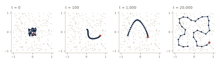
Such maps can fail by developing a kink: different parts of the map settle into different orientations, and the fold never straightens out however long training continues. The usual cure is to restart from new random weights with a wider initial window or a slower decay. Maps also have harmless ambiguities (a chain can run in either direction; a square grid can settle in any of eight orientations). Once trained, the target space can be clustered or labeled with a small amount of supervised data, which is one way SOMs are used for classification.
Clustering and dimensionality reduction
Clustering groups the rows of the \(n \times d\) data matrix (samples); dimensionality reduction can be seen as grouping its columns (features). Principal components find linear combinations that account for the variance of the features; factor analysis looks for a few hidden factors that account for the correlations between them (see Intro to ML, module 12). A clustering view gives a simple hierarchical procedure: use the squared correlation \(\rho_{ij}^2\) between features \(i\) and \(j\) (between 0 for uncorrelated and 1 for perfectly correlated features) as a similarity, merge the two most correlated features or groups of features, replace them by their average, and repeat until the desired number of features remains. Averaging assumes the features have comparable scales, so we standardize them first. Six features made from three hidden factors:
rngf = np.random.default_rng(1019)
Fac = rngf.normal(size=(300, 3))                        # three hidden factors
noise = lambda s: s * rngf.normal(size=300)
X_f = np.column_stack([Fac[:, 0] + noise(0.3), Fac[:, 0] + noise(0.4), Fac[:, 1] + noise(0.3),
                       Fac[:, 2] + noise(0.5), Fac[:, 1] + noise(0.5), Fac[:, 2] + noise(0.3)])
groups = [[i] for i in range(6)]
standardize = lambda M: (M - M.mean(axis=0)) / M.std(axis=0)
while len(groups) > 3:
    feats = np.array([standardize(X_f[:, g]).mean(axis=1) for g in groups])   # one averaged feature per group
    R2 = np.corrcoef(feats) ** 2
    np.fill_diagonal(R2, -1)
    i, j = sorted(np.unravel_index(R2.argmax(), R2.shape))
    print(f"merge {groups[i]} and {groups[j]} (squared correlation {R2[i, j]:.3f})")
    groups[i] = groups[i] + groups.pop(j)
print("final feature groups:", groups)
merge [0] and [1] (squared correlation 0.823)
merge [2] and [4] (squared correlation 0.793)
merge [3] and [5] (squared correlation 0.717)
final feature groups: [[0, 1], [2, 4], [3, 5]]
The procedure finds the three pairs of features driven by the same factor.
In practice. Unsupervised methods optimize representation: they favor directions and groupings with large variability. Classification needs discrimination: features along which the class means differ a lot relative to the within-class spread. The two often coincide, but nothing guarantees it; a set of clean, isolated clusters can each contain several classes. When labels are available, even a few, use them, through discriminant analysis or by labeling clusters, and remember that knowledge of the problem domain is usually the best source of good features.
Summary
| Method | What it assumes | How it works | Watch for |
|---|---|---|---|
| ML for mixtures (Case 1, EM) | known component forms, known \(c\), identifiable mixture | fixed-point equations: posterior-weighted frequencies, means, covariances | local maxima, saddles, singular solutions with free covariances |
| k-means | compact spherical clusters of similar size | nearest-mean assignment, recompute means; minimizes \(J_e\) locally | depends on start and on the units of the features |
| Fuzzy k-means | graded memberships, exponent \(b > 1\) | alternate weighted means and membership formula | memberships forced to sum to one over the \(c\) clusters |
| Unsupervised Bayesian learning | prior \(p(\boldsymbol{\theta})\) plus the mixture model | recursive posterior, multiply by the mixture density | \(c^n\) labelings, no sufficient statistic; decision-directed shortcut is biased |
| \(J_e\) / \(\operatorname{tr}\mathbf{S}_W\) | Euclidean geometry, similar cluster sizes | minimized by iterative transfers | not invariant to linear maps; splits large clusters |
| \(J_d\) and invariant criteria | compact clusters, nonsingular \(\mathbf{S}_W\) | functions of the eigenvalues of \(\mathbf{S}_W^{-1}\mathbf{S}_B\) | more local optima; agree with each other for \(c = 2\) |
| Agglomerative hierarchical | a cluster distance | merge nearest clusters; dendrogram; single = MST | chaining (single), splitting elongated clusters (complete) |
| Ward (stepwise optimal) | \(J_e\) | merge the pair with smallest \(d_e\) | good start for iterative optimization, not optimal |
| Leader–follower, ART | a threshold or vigilance | on-line: follow nearest center or create a new one | order of presentation; threshold sets \(c\) |
| MST clustering | clusters separated by long edges | Prim’s algorithm, delete long or inconsistent edges | one global threshold cannot fit clusters of different density |
| PCA, NLCA | representation by squared error | eigenvectors; linear or nonlinear autoencoder | largest variance need not be most discriminative |
| ICA | independent non-Gaussian sources, linear mixing | maximize output entropy (infomax), natural gradient | order, sign and scale ambiguity |
| MDS, SOM | dissimilarities; neighborhoods worth keeping | double centering; gradient on stress; winner and window updates | curved or non-Euclidean data cannot be flattened exactly; kinks |
Ideas to carry forward:
- Unsupervised learning of a mixture is supervised learning with each sample’s label replaced by its posterior probability. Everything follows from that: the gradient conditions, EM, k-means as the hard-assignment limit, and the dilution of the evidence from an unlabeled sample.
- A clustering is only as meaningful as its similarity measure and criterion. Units matter for \(J_e\); \(J_d\) and the eigenvalues of \(\mathbf{S}_W^{-1}\mathbf{S}_B\) remove that dependence at the price of harder optimization.
- Different procedures impose different shapes on clusters: single linkage and MSTs follow chains, complete linkage and \(J_e\) prefer compact balls. Know which shape your method prefers before trusting what it finds.
- How many clusters there are is a statistical question with no complete answer. Look for large gaps in criterion values or merge heights, and calibrate formal tests by simulating the null hypothesis.
Exercises
- Extend
binary_mixture_pmfto three binary features and two components with equal priors. Pick a parameter matrix, perturb one entry, and show numerically that no other parameter matrix (apart from swapping the two components) reproduces all eight probabilities; for instance, minimize the squared difference of the probability tables with a crude grid or random search and see that the minimum is at the original parameters. - Derive the EM updates for a normal mixture in which all components share one covariance matrix \(\boldsymbol{\Sigma}\). Show that the update is the posterior-weighted average of the per-component scatter, divided by \(n\), and explain why this model has no singular solutions when \(n > d\). Modify
em_gmmaccordingly and run it on the outlier data of this module. - Show that with \(c\) components the fixed-point iteration for the means started from \(\hat{\boldsymbol{\mu}}_1(0) = \cdots = \hat{\boldsymbol{\mu}}_c(0)\) reaches the sample mean in one step and stays there in exact arithmetic. Then show, for the 1-D example, that this point is a saddle of the log-likelihood by computing the Hessian numerically.
- For fuzzy k-means, show that as \(b \to 1^{+}\) the membership formula tends to the k-means indicator (assume no ties), and that as \(b \to \infty\) every membership tends to \(1/c\). What happens to the fuzzy means in the second limit?
- Prove the transfer rule for removing a sample from \(\mathcal{D}_i\), \(J_i^* = J_i - \frac{n_i}{n_i - 1}\lVert \hat{\mathbf{x}} - \mathbf{m}_i \rVert^2\). Then construct a small data set (a few points in one dimension suffice) and a k-means fixed point from which a single transfer still lowers \(J_e\).
- Show that the eigenvalues of \(\mathbf{S}_W^{-1}\mathbf{S}_B\) are unchanged by \(\mathbf{x} \mapsto \mathbf{A}\mathbf{x} + \mathbf{b}\) for nonsingular \(\mathbf{A}\), and that \(\mathbf{S}_B\) has rank at most \(c - 1\). Conclude that for \(c = 2\) all of \(J_d\), \(\operatorname{tr}\mathbf{S}_W^{-1}\mathbf{S}_B\), \(\operatorname{tr}\mathbf{S}_T^{-1}\mathbf{S}_W\) and \(\lvert \mathbf{S}_W \rvert / \lvert \mathbf{S}_T \rvert\) rank partitions identically.
- Use
all_criteriaon 12 points drawn from two well-separated Gaussians of very different sizes (say 9 and 3 points). Which criteria recover the natural partition for \(c = 2\)? Relate your findings to the warning about \(J_e\) and unequal cluster sizes. - Prove that the cophenetic distance of single-linkage and complete-linkage dendrograms is an ultrametric, and that every ultrametric satisfies the triangle inequality. Then show that single linkage run on the cophenetic distances of any single-linkage dendrogram reproduces the same dendrogram.
- Replace the inconsistent-edge rule by one that compares an edge with the average length of the edges within two steps of each end point, separately on each side, and requires it to exceed both averages by a factor \(r\). Test it on the three-density data for several \(r\).
- Implement competitive learning as DHS describe it (augment with \(x_0 = 1\), normalize samples and weights, dot-product winner) for \(c = 3\) on the three-group data, and compare the resulting centers with k-means. Then make the learning rate decay and add a fourth, far-away group of samples after convergence: can the network still learn it?
- Modify
infomax_naturalfor light-tailed sources by replacing the term \(\mathbf{1} - 2\mathbf{y}\) with \(\tanh(\mathbf{u}) - \mathbf{u}\) (the sub-Gaussian branch of the “extended infomax” rule), and test both versions on a sine wave mixed with a uniform noise source. Measure the excess kurtosis of each source first, and explain which version works and why. - In your own words: why can an unlabeled sample teach us less about \(\boldsymbol{\theta}\) than a labeled one, and under what circumstances would it teach us almost as much? Relate your answer to the overlap between the component densities and to the decision-directed bias experiment.
Going further
- R. O. Duda, P. E. Hart, and D. G. Stork, Pattern Classification, 2nd ed., chapter 10 — the source for this module. Problems 1–3 (identifiability), 6 and 11–17 (maximum-likelihood mixtures, fuzzy k-means and EM), 20–29 (criterion functions and invariants), 31 and 36 (transfer and Ward rules), 33–39 (hierarchical clustering and induced metrics), 40–41 (the validity test) and 44–50 (component analysis, ICA and MDS) pair with the sections above; Computer exercises 1–7 (mixtures, k-means, decision-directed learning), 9–12 (criteria and dendrograms), 14 (graph methods), 16 (ICA) and 17 (MDS) extend the code.
- Intro to ML, module 09 (k-means, Gaussian mixtures, and the general EM algorithm with its convergence proof) and Intro to ML, module 12 (PCA from two viewpoints, probabilistic PCA, factor analysis, kernel PCA, and FastICA).
- A. K. Jain and R. C. Dubes, Algorithms for Clustering Data, Prentice Hall, 1988 — a thorough classical treatment of similarity measures, hierarchical and partitional clustering, and cluster validity.
- A. J. Bell and T. J. Sejnowski, “An information-maximization approach to blind separation and blind deconvolution”, Neural Computation, 1995 — the infomax derivation of ICA used above.
- J. B. Kruskal, “Multidimensional scaling by optimizing goodness of fit to a nonmetric hypothesis”, Psychometrika, 1964 — stress and nonmetric MDS.
- T. Hastie, R. Tibshirani, and J. Friedman, The Elements of Statistical Learning, 2nd ed., chapter 14 — a modern survey of clustering, self-organizing maps, PCA, ICA and MDS, freely available from the authors.
These notes follow the chapters of R. O. Duda, P. E. Hart, and D. G. Stork, Pattern Classification, 2nd edition (Wiley, 2001), the course text. The explanations, code, figures, and exercises here are written for this course; the book remains the reference, with the full derivations, worked examples, and many more problems.