CSE 455/555 · Module 09 · Session 9
Algorithm-Independent Machine Learning
No free lunch and the ugly duckling, MDL and Occam's razor, bias and variance, jackknife and bootstrap, bagging and boosting, cross-validation and model comparison, and combining classifiers.
Companion reading: Duda, Hart & Stork, Pattern Classification, chapter 9, “Algorithm-Independent Machine Learning”
By the end of this module you can
- State the no free lunch theorem in terms of off-training-set error, prove its fixed-training-set part, and verify it by enumerating every target function on a small binary input space.
- Count the predicates shared by two patterns and explain why the ugly duckling theorem makes every notion of similarity depend on a choice of representation.
- Explain Kolmogorov complexity and the minimum description length principle, compute a two-part code length for a simple classifier, and relate MDL to MAP estimation and to Occam’s razor.
- Derive the bias–variance decomposition for regression and the boundary-error decomposition for classification, and measure both by simulating many training sets.
- Use the jackknife and the bootstrap to estimate the bias and variance of an arbitrary statistic, and check the estimates against a Monte Carlo ground truth.
- Implement bagging with decision trees and AdaBoost with decision stumps from scratch, prove the AdaBoost training-error bound, and explain what bagging and boosting do to bias and variance.
- Estimate and compare classifiers with cross-validation, leave-one-out, the bootstrap, likelihood-based and Bayesian model comparison, and learning-curve extrapolation, and compute the capacity of a separating hyperplane.
- Combine classifiers with a mixture of experts trained by gradient ascent, and with voting, Borda counts, and sum and product rules when the components give only labels or ranks.
Contents
- What “algorithm-independent” means
- Lack of inherent superiority of any classifier
- The ugly duckling theorem
- Minimum description length
- Overfitting avoidance and Occam’s razor
- Bias and variance
- Resampling for estimating statistics
- Resampling for classifier design
- Estimating and comparing classifiers
- Parametric models
- Cross-validation
- Jackknife and bootstrap estimates of accuracy
- Maximum-likelihood model comparison
- Bayesian model comparison and the Occam factor
- Bayesian model selection and no free lunch
- The problem-average error rate
- Predicting final performance from learning curves
- The capacity of a separating plane
- Combining classifiers
- Summary
- Exercises
- Going further
Eight modules in, we have a toolbox: Bayes decision rules and their error bounds (module 02), maximum-likelihood and Bayesian parameter estimates (module 03), Parzen windows and nearest neighbors (module 04), linear machines (module 05), multilayer networks (module 06), stochastic search (module 07), and trees and grammars (module 08). Faced with a new problem, which one should we pick? Is there a best one? This module steps back from individual methods and asks what can be said about learning in general, whatever the algorithm.
The answers come in three kinds. First, some limits: the no free lunch theorem says that no learning algorithm beats any other when we average over all possible problems, and the ugly duckling theorem says the same of feature representations and similarity. Whatever advantage a method has comes from assumptions that match the problem. Second, some ways to describe that match: description length, and above all bias and variance. Third, techniques that work with any classifier: the jackknife and bootstrap for estimating statistics, bagging and boosting for building better classifiers out of weaker ones, cross-validation and model comparison for estimating and choosing classifiers, and methods for combining classifiers.
The chapter we follow is chapter 9 of Duda, Hart & Stork, Pattern Classification (2nd ed., 2001), which we abbreviate DHS. The CSE 474/574 notes cover some of the same ground from Bishop’s point of view: the regression bias–variance decomposition and the Bayesian evidence in Intro to ML, module 03, and committees, boosting, trees, and mixtures of experts in Intro to ML, module 14. Those notes write transposes as \(^{\mathrm{T}}\) and classes as \(\mathcal{C}_k\); here we keep DHS’s \(^{t}\) and \(\omega_j\).
What “algorithm-independent” means
The phrase has two meanings in this module. The first is results that hold for every learning algorithm: the no free lunch theorem, the ugly duckling theorem, and the bias–variance decompositions are statements about learning as such, and they apply equally to a neural network, a nearest-neighbor rule, or a Gaussian classifier fitted by maximum likelihood. The second is procedures that can be wrapped around any learning algorithm: resampling, cross-validation, boosting, and classifier combination take a training method as a black box. Of course these procedures are algorithms too; what makes them “algorithm-independent” is that they do not care what is inside the box.
One thing we will not get is a way to rank algorithms in the abstract. The Bayes error of module 02 is a hard floor for every classifier, but we rarely know it, and knowing it would not tell us how to design a classifier. The tools in this module instead help us find out, on the problem at hand, how well a classifier is doing and whether another would do better.
All the code in this module uses NumPy, with SciPy for a few special functions. The first cell sets up the imports and a seeded generator.
import itertools
import zlib
from math import comb

import numpy as np
from scipy.special import expit, gammaln, logsumexp, ndtr, ndtri

np.set_printoptions(precision=4, suppress=True)
rng = np.random.default_rng(455)
Lack of inherent superiority of any classifier
Suppose all we care about is how well a classifier does on new patterns. If we make no assumptions about the problem, is there any reason to prefer one learning algorithm to another, or even to prefer any algorithm to random guessing? The answer, perhaps surprisingly, is no.
Off-training-set error
To make the question precise we need to be careful about what “new patterns” means. In the earlier modules we measured performance on a test set drawn from the same distribution as the training set. On a discrete input space with a lot of data, such a test set contains many patterns that also appear in the training set, and any algorithm that memorizes its training data gets those right for free. To compare the ability of algorithms to generalize, we should score them only on patterns they have not seen. The off-training-set error is the error rate on the inputs that do not appear in the training set \(\mathcal{D}\).
Take a two-category problem on a finite input space. The training set \(\mathcal{D}\) consists of \(n\) patterns \(\mathbf{x}^i\) with labels \(y_i = F(\mathbf{x}^i) \in \{+1, -1\}\), where \(F\) is the unknown target function we are trying to learn. (For now \(F\) is deterministic, so there is no Bayes error; the results carry over to noisy targets.) A learning algorithm, given \(\mathcal{D}\), produces a hypothesis \(h\); a deterministic algorithm always produces the same \(h\) from the same \(\mathcal{D}\), while a stochastic one (a network trained from random initial weights, say) produces \(h\) with some probability \(P(h \mid \mathcal{D})\). With input distribution \(P(\mathbf{x})\), the expected off-training-set error of algorithm \(k\) on target \(F\) with training set \(\mathcal{D}\) is
\[\mathcal{E}_k(E \mid F, \mathcal{D}) = \frac{\sum_{\mathbf{x} \notin \mathcal{D}} P(\mathbf{x}) \sum_h \left[1 - \delta\big(F(\mathbf{x}), h(\mathbf{x})\big)\right] P_k(h \mid \mathcal{D})}{\sum_{\mathbf{x} \notin \mathcal{D}} P(\mathbf{x})},\]where \(\delta(a, b)\) is 1 when \(a = b\) and 0 otherwise. The denominator normalizes to an error rate on the unseen inputs; DHS leave it out, which changes nothing below. Averaging over the training sets that \(F\) can generate gives \(\mathcal{E}_k(E \mid F, n)\), the expected off-training-set error for training sets of size \(n\).
The theorem
Result. No free lunch. Take two learning algorithms \(P_1(h \mid \mathcal{D})\) and \(P_2(h \mid \mathcal{D})\). Whatever the input distribution \(P(\mathbf{x})\) and the training-set size \(n\):
- Averaged uniformly over all target functions \(F\), \(\mathcal{E}_1(E \mid F, n) - \mathcal{E}_2(E \mid F, n) = 0\).
- For any fixed training set \(\mathcal{D}\), averaged uniformly over all \(F\) consistent with it, \(\mathcal{E}_1(E \mid F, \mathcal{D}) - \mathcal{E}_2(E \mid F, \mathcal{D}) = 0\).
- Averaged uniformly over all priors \(P(F)\), \(\mathcal{E}_1(E \mid n) - \mathcal{E}_2(E \mid n) = 0\).
- For any fixed \(\mathcal{D}\), averaged uniformly over all priors \(P(F)\), \(\mathcal{E}_1(E \mid \mathcal{D}) - \mathcal{E}_2(E \mid \mathcal{D}) = 0\).
Part 2 has a two-line proof, and it shows where the theorem comes from. Fix \(\mathcal{D}\). The targets consistent with \(\mathcal{D}\) agree on the training inputs and take every possible combination of values on the inputs outside \(\mathcal{D}\). So under the uniform average, for each \(\mathbf{x} \notin \mathcal{D}\) the value \(F(\mathbf{x})\) is \(+1\) for exactly half of the targets and \(-1\) for the other half, whatever happens at the other inputs. The hypothesis \(h\) depends on \(\mathcal{D}\) only, so it cannot depend on \(F(\mathbf{x})\) there, and it is wrong for exactly half of the targets:
\[\frac{1}{\#F} \sum_{F} \left[1 - \delta\big(F(\mathbf{x}), h(\mathbf{x})\big)\right] = \frac{1}{2} \qquad \text{for every } h \text{ and every } \mathbf{x} \notin \mathcal{D}.\]Plugging this into \(\mathcal{E}_k\) gives \(\tfrac{1}{2}\) for every algorithm. Part 1 follows by averaging part 2 over the training sets: for a fixed set of training inputs, grouping the targets by their values on those inputs gives groups in which part 2 applies. Parts 3 and 4 say the same thing one level up, for priors over targets; averaging over all priors uniformly amounts to a uniform average over targets again.
In words: if every target function is equally likely, the training data say nothing at all about the labels of unseen patterns. An algorithm we think of as good, one we think of as bad, and a coin flip all have off-training-set error one half. Any claim that algorithm 1 is better than algorithm 2 is a claim about which targets are likely.
An exhaustive check on a binary cube
We can verify the theorem by brute force on a small input space: the \(2^4 = 16\) binary vectors with \(d = 4\) features, each equally likely. There are \(2^{16} = 65{,}536\) target functions, few enough to enumerate. We compare four deterministic algorithms:
- majority: predict the more common label in the training set, for every input;
- nearest neighbor: predict the label of the nearest training pattern in Hamming distance (ties are settled by a vote among the tied neighbors);
- anti-nearest neighbor: predict the opposite of the nearest-neighbor label, a deliberately perverse rule;
- constant: always predict \(+1\).
A deterministic algorithm sees only the \(n\) training labels, so it can produce at most \(2^n\) different hypotheses. The helper below computes each algorithm’s predictions once for every possible training labeling and then looks them up for all 65,536 targets at once.
d_cube = 4
X_cube = np.array(list(itertools.product([0, 1], repeat=d_cube)))   # 16 patterns
n_pat = len(X_cube)
hamming = (X_cube[:, None, :] != X_cube[None, :, :]).sum(axis=2)

def all_labelings(m):
    """All 2^m labelings of m items, as rows of +1/-1 (row k spells out the bits of k)."""
    bits = (np.arange(2**m)[:, None] >> np.arange(m)) & 1
    return 2 * bits - 1

def alg_majority(tr, y_tr, te):
    return np.full(len(te), 1 if y_tr.sum() >= 0 else -1)

def alg_nn(tr, y_tr, te):
    D = hamming[np.ix_(te, tr)]
    tied = D == D.min(axis=1, keepdims=True)   # all training points at the nearest distance
    return np.where((tied * y_tr).sum(axis=1) >= 0, 1, -1)

def alg_anti_nn(tr, y_tr, te):
    return -alg_nn(tr, y_tr, te)

def alg_constant(tr, y_tr, te):
    return np.ones(len(te), dtype=int)

algorithms = {"majority": alg_majority, "nearest neighbor": alg_nn,
              "anti-nearest neighbor": alg_anti_nn, "constant +1": alg_constant}

def ots_error(alg, tr, targets):
    """Off-training-set error rate of a deterministic algorithm for each target (row), P(x) uniform."""
    te = np.setdiff1d(np.arange(n_pat), tr)
    labs = all_labelings(len(tr))
    preds = np.array([alg(tr, yl, te) for yl in labs])    # one hypothesis per training labeling
    idx = ((targets[:, tr] + 1) // 2) @ (1 << np.arange(len(tr)))
    return (preds[idx] != targets[:, te]).mean(axis=1)

targets_all = all_labelings(n_pat)          # 65,536 targets x 16 inputs
tr_fixed = np.array([0, 3, 5, 6, 9, 15])    # a training set of n = 6 inputs
idx_tr = ((targets_all[:, tr_fixed] + 1) // 2) @ (1 << np.arange(6))
print(f"{len(targets_all)} targets; each training labeling is shared by "
      f"{np.bincount(idx_tr).min()} of them")
for name, alg in algorithms.items():
    e = ots_error(alg, tr_fixed, targets_all)
    group_means = np.bincount(idx_tr, weights=e) / np.bincount(idx_tr)
    print(f"{name:22s} mean over consistent targets: min {group_means.min():.4f}, "
          f"max {group_means.max():.4f}")
65536 targets; each training labeling is shared by 1024 of them
majority               mean over consistent targets: min 0.5000, max 0.5000
nearest neighbor       mean over consistent targets: min 0.5000, max 0.5000
anti-nearest neighbor  mean over consistent targets: min 0.5000, max 0.5000
constant +1            mean over consistent targets: min 0.5000, max 0.5000
For each of the 64 ways the six training patterns can be labeled, the \(2^{10} = 1024\) targets consistent with that labeling give each algorithm an average off-training-set error of exactly one half. That is part 2 of the theorem. Part 1 averages over training sets as well; we check it for 20 random training sets of each of several sizes, and also count how often nearest neighbor beats majority on individual targets.
rng_nfl = np.random.default_rng(9)
for n_tr in (2, 6, 10):
    avg = {name: 0.0 for name in algorithms}
    wins = losses = 0
    for _ in range(20):
        tr = np.sort(rng_nfl.choice(n_pat, size=n_tr, replace=False))
        errs = {name: ots_error(alg, tr, targets_all) for name, alg in algorithms.items()}
        for name in algorithms:
            avg[name] += errs[name].mean() / 20
        wins += np.sum(errs["nearest neighbor"] < errs["majority"])
        losses += np.sum(errs["nearest neighbor"] > errs["majority"])
    print(f"n = {n_tr:2d}: " + ", ".join(f"{v:.4f}" for v in avg.values())
          + f"   NN beats majority on {wins} target/set pairs, loses on {losses}")
n =  2: 0.5000, 0.5000, 0.5000, 0.5000   NN beats majority on 321536 target/set pairs, loses on 321536
n =  6: 0.5000, 0.5000, 0.5000, 0.5000   NN beats majority on 480212 target/set pairs, loses on 480212
n = 10: 0.5000, 0.5000, 0.5000, 0.5000   NN beats majority on 440314 target/set pairs, loses on 440314
Every algorithm averages exactly one half, including the perverse one, and nearest neighbor beats majority on exactly as many (target, training set) pairs as it loses. The last fact is a small instance of a general symmetry: flipping the labels of all the unseen inputs leaves every algorithm’s hypothesis unchanged and turns each off-training-set error \(e\) into \(1 - e\), so wins and losses pair up one to one.
Conservation of generalization
The same symmetry gives a “conservation law”: for every algorithm, the off-training-set accuracy minus one half, summed over all targets, is zero. An algorithm can do better than chance on some targets only by doing correspondingly worse on others. It can trade a large gain on a few targets for a small loss on many, or a moderate gain on many for a large loss on a few, but it cannot gain everywhere, and it cannot gain somewhere while breaking even everywhere else.
Two practical lessons follow. When one algorithm beats another in a study, the result is evidence about the kind of problems in the study, not about the algorithms in general. And every algorithm, however well founded, has problems on which it does badly; being able to try several kinds of classifiers is the best protection.
Watch out. The theorem is about the uniform average over targets. Real problems are not drawn uniformly from all possible functions: nearby patterns usually have the same label, and targets usually depend on few features in simple ways. The theorem does not say that learning is hopeless. It says that learning works only because of assumptions like these, and that an algorithm’s success measures how well its assumptions match the problem.
The ugly duckling theorem
The no free lunch theorem says that no algorithm is privileged. The ugly duckling theorem says the same about features and about similarity between patterns: without assumptions, there is no best representation, and no two patterns are more alike than any other two.
Predicates and their rank
Describe patterns by \(d\) binary features \(f_1, \dots, f_d\). A pattern is one of the possible feature combinations; with no constraints between features there are \(2^d\) of them, and we can draw them as the regions of a Venn diagram, one circle per feature. Constraints remove regions: if \(f_1\) is “is a square” and \(f_2\) is “is a rectangle”, the region “square but not a rectangle” is empty.
A predicate is any statement that is true of some patterns and false of the others, such as “\(f_1\) AND NOT \(f_2\)” or “\(f_1\) OR \(f_3\)”. Since a predicate is determined by the set of patterns for which it is true, the predicates on \(m\) possible patterns correspond one to one with the subsets of those patterns, and there are
\[\sum_{r=0}^{m} \binom{m}{r} = (1 + 1)^m = 2^m\]of them. The rank \(r\) of a predicate is the number of patterns it is true of; there are \(\binom{m}{r}\) predicates of rank \(r\). Rank 1 predicates pick out single patterns, and the one predicate of rank \(m\) is always true.
Counting shared predicates
The most obvious measure of how similar two patterns are is the number of features they share. The ugly duckling theorem looks at a more general measure, the number of predicates they share, since predicates include features, their negations, and every logical combination of them.
Take two distinct patterns \(\mathbf{x}_i\) and \(\mathbf{x}_j\). A predicate is true of both exactly when its subset contains both. Such a subset contains \(\mathbf{x}_i\) and \(\mathbf{x}_j\) plus any selection of the other \(m - 2\) patterns, so the number of shared predicates of rank \(r\) is \(\binom{m - 2}{r - 2}\), and the total is
\[\sum_{r=2}^{m} \binom{m-2}{r-2} = 2^{m-2}.\]This does not depend on which two patterns we picked.
Result. Ugly duckling. Given any finite collection of predicates rich enough to distinguish every pair of patterns, all pairs of distinct patterns have the same number of predicates in common. If similarity is measured by shared predicates, any two distinct patterns are equally similar.
The name comes from the conclusion that, measured this way, an ugly duckling is exactly as similar to a swan as two swans are to each other. We check the count by enumeration, with \(d = 3\) features and \(m = 8\) patterns, and compare it with the count of shared features.
d_u = 3
patt = np.array(list(itertools.product([0, 1], repeat=d_u)))    # the 8 patterns
m_u = len(patt)
pred = (np.arange(2**m_u)[:, None] >> np.arange(m_u)) & 1         # 256 predicates x 8 patterns
shared_pred = pred.T @ pred                                      # predicates true of both i and j
shared_feat = (patt[:, None, :] == patt[None, :, :]).sum(axis=2)
off = ~np.eye(m_u, dtype=bool)
print("predicates by rank:", np.bincount(pred.sum(axis=1)))
print(f"shared predicates, distinct pairs: min {shared_pred[off].min()}, "
      f"max {shared_pred[off].max()}  (2^(m-2) = {2**(m_u - 2)})")
print(f"shared features, distinct pairs:   min {shared_feat[off].min()}, "
      f"max {shared_feat[off].max()}")

allowed = np.array([0, 1, 3, 4, 7])       # a constrained problem: only 5 patterns can occur
pred_c = (np.arange(2**len(allowed))[:, None] >> np.arange(len(allowed))) & 1
sp = pred_c.T @ pred_c
print(f"with {len(allowed)} allowed patterns: {len(pred_c)} predicates, "
      f"each distinct pair shares {sp[~np.eye(len(allowed), dtype=bool)].min()}-"
      f"{sp[~np.eye(len(allowed), dtype=bool)].max()}")
predicates by rank: [ 1  8 28 56 70 56 28  8  1]
shared predicates, distinct pairs: min 64, max 64  (2^(m-2) = 64)
shared features, distinct pairs:   min 0, max 2
with 5 allowed patterns: 32 predicates, each distinct pair shares 8-8
The rank counts are the binomial coefficients \(\binom{8}{r}\), every distinct pair shares exactly 64 predicates, and shared features range from 0 to 2. With constraints only the allowed patterns count, \(m\) drops to 5, and every pair shares \(2^{3} = 8\) predicates. The theorem holds for any Venn diagram, constrained or not.
Features are a choice
Counting shared features does distinguish between pairs, but only because it singles out one particular set of predicates, the features, as the ones that matter. That choice is an assumption. An invertible re-encoding of the same patterns keeps all the information but changes which patterns share features. For example, replace \((f_1, f_2, f_3)\) by \((f_1,\ f_1 \oplus f_2,\ f_2 \oplus f_3)\), where \(\oplus\) is exclusive or.
def recode(p):
    return np.array([p[0], p[0] ^ p[1], p[1] ^ p[2]])

a, b, c = np.array([0, 0, 0]), np.array([1, 1, 1]), np.array([1, 0, 0])
for label, enc in [("original", lambda p: p), ("recoded ", recode)]:
    ea, eb, ec = enc(a), enc(b), enc(c)
    print(f"{label}: a={ea}, b={eb}, c={ec};  Hamming(a, b) = {np.sum(ea != eb)}, "
          f"Hamming(a, c) = {np.sum(ea != ec)}")
recoded_all = np.array([recode(p) for p in patt])
print("recoding is one to one:", len({tuple(r) for r in recoded_all}) == m_u)
original: a=[0 0 0], b=[1 1 1], c=[1 0 0];  Hamming(a, b) = 3, Hamming(a, c) = 1
recoded : a=[0 0 0], b=[1 0 0], c=[1 1 0];  Hamming(a, b) = 1, Hamming(a, c) = 2
recoding is one to one: True
In the original features \(c\) is much closer to \(a\) than \(b\) is; after recoding, \(b\) is the closer one. Neither encoding is more correct than the other without knowledge of the problem. So even the notion that two patterns are “similar”, which nearest-neighbor rules, clustering, and most of our intuition rely on, rests on assumptions about which features matter. The same argument applies to continuous features once they are discretized, at any resolution.
Minimum description length
A common argument for simple classifiers goes like this: the patterns in a category share some essential structure (the signal) and differ in accidental ways (the noise), so a classifier that describes the category as compactly as possible keeps the signal and discards the noise. The minimum description length principle makes this argument precise. To state it we first need a measure of how complex a description is.
Algorithmic complexity
Suppose a sender wants to transmit a binary string \(x\) and both sides have agreed on a decoding method \(L\). The sender transmits some shorter string \(y\) with \(L(y) = x\), and the cost is the length \(\lvert y \rvert\) in bits. The best achievable cost with this method is the length of the shortest such \(y\). The trouble is that it depends on the method: a decoder designed for \(x\) could produce it from a single bit.
Algorithmic complexity, also called Kolmogorov complexity, removes that dependence by letting the decoder be a universal computer, one that can run any program. The Kolmogorov complexity of \(x\) is the length of the shortest program that prints \(x\) and halts:
\[K(x) = \min_{y :\, U(y) = x} \lvert y \rvert,\]where \(U\) is a fixed universal Turing machine. Changing to a different universal machine changes \(K(x)\) by at most an additive constant (the length of a program that makes one machine imitate the other), so \(K\) is a property of \(x\) up to that constant. It measures how incompressible \(x\) is.
Some examples. A string of \(n\) ones is simple: a fixed loop plus the number \(n\), which takes about \(\log_2 n\) bits, so \(K(x) = O(\log_2 n)\). The first \(n\) binary digits of \(\pi\) look random but come from a fixed program that computes \(\pi\) plus the number \(n\), again about \(\log_2 n\) bits; the digit sequence itself has almost no information. A string of \(n\) fair coin flips, with high probability, has no description much shorter than itself: \(K(x) \approx n\).
\(K\) cannot be computed (no program can find the shortest program for every string), but any compressor gives an upper bound: the compressed file plus the fixed decompressor is a program that prints \(x\). The cell below uses zlib.
def zlib_bits(bits):
    """Bits in the zlib-compressed string: an upper bound on K(x), up to a constant."""
    return 8 * len(zlib.compress(np.packbits(bits).tobytes(), 9))

rng_k = np.random.default_rng(2024)
print("      n    ones   period-3   coin flips")
for n_bits in (1_000, 10_000, 100_000):
    ones = np.ones(n_bits, dtype=np.uint8)
    period3 = np.resize(np.array([1, 0, 1], dtype=np.uint8), n_bits)
    coins = rng_k.integers(0, 2, n_bits).astype(np.uint8)
    print(f"{n_bits:7d} {zlib_bits(ones):7d} {zlib_bits(period3):9d} {zlib_bits(coins):11d}")
      n    ones   period-3   coin flips
   1000      96       112        1088
  10000     152       168       10088
 100000     280       320      100088
The regular strings compress to a tiny fraction of their length (a better compressor would get the ones down to about \(\log_2 n\) bits), while the coin flips do not compress at all; the few extra bits are zlib’s overhead. There is an irony in the last column: those “coin flips” came from a seeded pseudo-random generator, so a program of a few hundred bits (the generator plus the seed) prints them. Their true Kolmogorov complexity is small, and zlib cannot find the short description. That is the practical face of uncomputability: we can bound \(K\) from above but never know how far above we are.
The minimum description length principle
Now describe a classifier \(h\) and the training data \(\mathcal{D}\) as binary strings. The minimum description length (MDL) principle says we should choose the hypothesis that minimizes the total length of a two-part description, first the hypothesis and then the data encoded with its help:
\[K(h, \mathcal{D}) = K(h) + K(\mathcal{D} \text{ using } h), \qquad h^* = \arg\min_h K(h, \mathcal{D}).\]A complex hypothesis costs many bits to state but may make the data cheap to encode; a simple one is cheap to state but leaves many exceptions to spell out. MDL balances the two. Variants weight the two terms differently.
In practice we replace \(K\) by the length of a concrete code. Decision trees are the classic case, as in module 08: the tree costs bits in proportion to its number of nodes, and the labels given the tree cost bits in proportion to the entropy at the leaves, so pruning a tree by an entropy criterion minimizes a description length of this form.
We try the principle on a simpler classifier that has the same flavor. The input is one-dimensional, \(x \in [0, 1]\), and the classifier cuts the interval into \(m\) equal cells and labels each cell by the majority class of its training points. The receiver knows the inputs \(x_i\) and needs the labels. Our code has two parts:
- the hypothesis: one bit per cell for its label (plus the choice of \(m\) from a fixed list of candidates, which costs the same for every \(m\) and can be dropped);
- the data given the hypothesis: in cell \(j\), with \(n_j\) points of which \(e_j\) disagree with the cell’s label, send \(e_j\) (which takes \(\log_2(n_j + 1)\) bits, since it is one of \(n_j + 1\) values) and then which \(e_j\) of the \(n_j\) points are the exceptions (\(\log_2 \binom{n_j}{e_j}\) bits).
The true posterior \(P(\omega_1 \mid x)\) is piecewise constant with four pieces, so we can compute the exact error of each fitted classifier.
edges_true = np.array([0.0, 0.3, 0.55, 0.7, 1.0])
post_true = np.array([0.85, 0.2, 0.8, 0.15])       # P(omega_1 | x) on each piece

def post_1d(x):
    return post_true[np.searchsorted(edges_true, x, side="right") - 1]

rng_m = np.random.default_rng(31)
n_m = 200
x_m = rng_m.uniform(0, 1, n_m)
y_m = (rng_m.uniform(0, 1, n_m) < post_1d(x_m)).astype(int)   # 1 = omega_1
x_fine = (np.arange(20000) + 0.5) / 20000                       # for the exact error integral

def log2_binom(n, k):
    return (gammaln(n + 1) - gammaln(k + 1) - gammaln(n - k + 1)) / np.log(2)

def cell_classifier(m, x, y):
    cell = np.minimum((x * m).astype(int), m - 1)
    n1 = np.bincount(cell, weights=y, minlength=m)
    nj = np.bincount(cell, minlength=m).astype(float)
    return (2 * n1 >= nj).astype(int), n1, nj       # label 1 on ties (and empty cells)

def description_length(m, x, y):
    lab, n1, nj = cell_classifier(m, x, y)
    e = np.where(lab == 1, nj - n1, n1)               # exceptions in each cell
    L_model = m                                       # one bit per cell label
    L_data = np.sum(np.log2(nj + 1) + log2_binom(nj, e))
    return L_model, L_data

def true_error_cells(m, x, y):
    lab, _, _ = cell_classifier(m, x, y)
    pred = lab[np.minimum((x_fine * m).astype(int), m - 1)]
    p1 = post_1d(x_fine)
    return np.mean(np.where(pred == 1, 1 - p1, p1))

print("   m   L(h)   L(D|h)   total   true error")
table = []
for m in (1, 2, 3, 4, 5, 6, 8, 10, 12, 16, 20, 30, 40, 60):
    Lh, Ld = description_length(m, x_m, y_m)
    table.append((m, Lh + Ld, true_error_cells(m, x_m, y_m)))
    print(f"{m:4d} {Lh:6d} {Ld:8.1f} {Lh + Ld:7.1f}   {table[-1][2]:.4f}")
m_mdl = min(table, key=lambda t: t[1])[0]
m_best = min(table, key=lambda t: t[2])[0]
bayes_1d = np.mean(np.minimum(post_1d(x_fine), 1 - post_1d(x_fine)))
print(f"MDL picks m = {m_mdl}; the lowest true error is at m = {m_best}; "
      f"Bayes error = {bayes_1d:.4f}")
   m   L(h)   L(D|h)   total   true error
   1      1    203.4   204.4   0.4700
   2      2    199.6   201.6   0.3800
   3      3    176.9   179.9   0.2800
   4      4    167.3   171.3   0.2700
   5      5    175.7   180.7   0.3300
   6      6    168.3   174.3   0.2400
   8      8    169.8   177.8   0.2800
  10     10    158.4   168.4   0.2000
  12     12    166.6   178.6   0.2450
  16     16    170.8   186.8   0.1925
  20     20    164.5   184.5   0.1700
  30     30    174.4   204.4   0.1800
  40     40    170.2   210.2   0.1875
  60     60    178.1   238.1   0.2467
MDL picks m = 10; the lowest true error is at m = 20; Bayes error = 0.1700
The data cost tends to fall as cells are added, though not steadily: a cell that straddles a change in the posterior mixes the classes and costs extra exceptions, so the column goes up and down with how well the cell edges happen to line up with the true pieces. The model cost grows linearly, and each extra cell also adds a \(\log_2(n_j + 1)\) term for its exception count, a price per parameter much like the one in the BIC we meet later. MDL picks \(m = 10\), with true error 0.200. The best value in the list, \(m = 20\), has cell edges that line up exactly with the true pieces and reaches the Bayes error of 0.17; MDL cannot know that. What it does do is stay well away from the large-\(m\) end of the table, where the error climbs again.
MDL and Bayes
MDL has a direct Bayesian reading. For discrete hypotheses, Bayes’ formula gives \(P(h \mid \mathcal{D}) = P(h) P(\mathcal{D} \mid h) / P(\mathcal{D})\), so the MAP hypothesis is
\[h^* = \arg\max_h \left[\log_2 P(h) + \log_2 P(\mathcal{D} \mid h)\right] = \arg\min_h \left[-\log_2 P(h) - \log_2 P(\mathcal{D} \mid h)\right].\]Shannon’s coding theorem says that an outcome of probability \(p\) can be encoded in about \(-\log_2 p\) bits and no fewer on average. So \(-\log_2 P(\mathcal{D} \mid h)\) is the length of the data encoded with \(h\)’s help, and \(-\log_2 P(h)\) is a code length for \(h\). Conversely, any prefix code for hypotheses defines a prior \(P(h) \propto 2^{-L(h)}\). Minimizing total description length is MAP estimation with a prior that favors short descriptions. Our cell classifier uses the prior \(2^{-m}\) on the cell labels, and the exception code is a likelihood.
This view makes two things clear. MDL is not assumption-free: the choice of code is the choice of prior, and it often turns out easier to think about a prior as a code length than as a distribution. And MDL is consistent: with enough data, it converges to the true model when the true model is among the candidates. What it cannot do is guarantee better performance at a finite sample size; that would contradict the no free lunch theorem.
Overfitting avoidance and Occam’s razor
Throughout the course we have fought overfitting with regularization, pruning, penalty terms, early stopping, and description lengths. The no free lunch theorem seems to undercut all of them: if no algorithm is better than another on average, why should preferring simpler classifiers help?
The resolution is that overfitting avoidance is itself a bias, a preference for some hypotheses over others. It helps on problems where simple hypotheses are more likely to be right and hurts on problems where they are not. The principle known as Occam’s razor, originally a counsel not to multiply entities beyond necessity, is read in pattern recognition as “do not use a classifier more complex than the training data require”. Under the uniform prior of the no free lunch theorem it has no advantage. Its empirical success says something about the problems we meet, not about learning in general.
We can see this with the binary cube from the no free lunch section. Replace the uniform average over all targets by averages over two small families of targets:
- one-feature targets, \(F(\mathbf{x}) = \pm(2x_j - 1)\) for some feature \(j\): 8 targets, all of them very “smooth”, since neighbors in Hamming distance usually share a label;
- parity targets, \(F(\mathbf{x}) = \pm(-1)^{\sum_{j \in S} x_j}\) for a subset \(S\) of at least three features: 10 targets in which flipping a relevant feature always flips the label.
single = np.array([s * (2 * X_cube[:, j] - 1) for j in range(d_cube) for s in (1, -1)])
parity = np.array([s * (-1) ** X_cube[:, list(S)].sum(axis=1)
                   for r in (3, 4) for S in itertools.combinations(range(d_cube), r)
                   for s in (1, -1)])
rng_o = np.random.default_rng(12)
train_sets = [np.sort(rng_o.choice(n_pat, size=6, replace=False)) for _ in range(200)]
print(f"{'':22s} {'uniform':>8s} {'one-feature':>12s} {'parity':>8s}")
for name, alg in algorithms.items():
    row = [np.mean([ots_error(alg, tr, T).mean() for tr in train_sets[:40]])
           for T in (targets_all, single, parity)]
    print(f"{name:22s} {row[0]:8.4f} {row[1]:12.4f} {row[2]:8.4f}")
                        uniform  one-feature   parity
majority                 0.5000       0.5675   0.5860
nearest neighbor         0.5000       0.2263   0.8005
anti-nearest neighbor    0.5000       0.7737   0.1995
constant +1              0.5000       0.5000   0.5000
Under the uniform prior all four algorithms tie at one half. When the targets are smooth, nearest neighbor wins and its perverse twin loses; when the targets are parities, the ranking is reversed. The constant rule stays at exactly one half, since every target in both families labels half the cube \(+1\). Majority does slightly worse than one half on both families, for the same reason: whichever label is more common among the six training patterns is less common among the ten unseen ones. Nothing about nearest neighbor made it better; its assumption that similar inputs have similar labels happened to match one family of targets.
Why, then, does Occam’s razor work so often in practice? DHS suggest several reasons, all of them about us rather than about mathematics. Perceptual systems shaped by evolution face strong pressure to be computationally cheap, so the problems we find natural and choose to study may be those that simple recognizers can solve. Researchers try simple methods before complex ones and stop when a method is good enough (a strategy called satisficing), so the recorded successes are biased toward problems that simple methods handle. And if we insist that more training data should not, on average, make a classifier worse, a version of Occam’s razor can be derived, but that insistence is itself a nonuniform prior over targets. Finally, as a consequence of the no free lunch theorem, the training data alone cannot tell us on which new problems a classifier will generalize well and on which it will not.
Bias and variance
Since no classifier is best in general, we need ways to describe how well a particular learning algorithm matches a particular problem. Two quantities do this: the bias, which measures how accurate the match is (high bias means a poor match), and the variance, which measures how precise it is (high variance means the learned classifier changes a lot from one training set to the next). They are not independent. Making an algorithm more flexible generally lowers its bias and raises its variance, and the art is in finding the balance. Intro to ML, module 03 derives the regression decomposition from Bishop’s side with regularized least squares; here we derive it in DHS’s form and then carry the idea over to classification, where it behaves quite differently.
Bias and variance for regression
Let \(F(x)\) be a real-valued target function and let each training set \(\mathcal{D}\) contain \(n\) noisy samples \(y = F(x) + \varepsilon\), with \(\varepsilon\) of mean zero and variance \(\sigma^2\). A learning algorithm turns \(\mathcal{D}\) into an estimate \(g(x; \mathcal{D})\). Different training sets give different estimates, so at a fixed \(x\) the estimate is a random variable, and we judge the algorithm by its mean-square deviation from \(F(x)\) averaged over training sets of size \(n\).
To split this error in two, add and subtract the average estimate \(\bar{g}(x) = \mathcal{E}_{\mathcal{D}}[g(x; \mathcal{D})]\) inside the square:
\[\begin{aligned} \mathcal{E}_{\mathcal{D}}\left[(g(x; \mathcal{D}) - F(x))^2\right] &= \mathcal{E}_{\mathcal{D}}\left[\big((g - \bar{g}) + (\bar{g} - F)\big)^2\right] \\ &= \mathcal{E}_{\mathcal{D}}\left[(g - \bar{g})^2\right] + 2(\bar{g} - F)\,\mathcal{E}_{\mathcal{D}}[g - \bar{g}] + (\bar{g} - F)^2 . \end{aligned}\]The middle term vanishes because \(\mathcal{E}_{\mathcal{D}}[g - \bar{g}] = 0\), and \(\bar{g} - F\) does not depend on \(\mathcal{D}\). So
Result. For every \(x\), with \(\bar{g}(x) = \mathcal{E}_{\mathcal{D}}[g(x; \mathcal{D})]\),
\[\mathcal{E}_{\mathcal{D}}\left[(g(x; \mathcal{D}) - F(x))^2\right] = \underbrace{\left(\bar{g}(x) - F(x)\right)^2}_{\text{bias}^2} + \underbrace{\mathcal{E}_{\mathcal{D}}\left[\left(g(x; \mathcal{D}) - \bar{g}(x)\right)^2\right]}_{\text{variance}} .\]The expected squared error on a new noisy target \(y\) adds the noise variance: \(\mathcal{E}[(g - y)^2] = \text{bias}^2 + \text{variance} + \sigma^2\).
The noise term follows the same way: \(g - y = (g - F) - \varepsilon\), and the cross term vanishes because the test noise \(\varepsilon\) has mean zero and is independent of \(\mathcal{D}\).
The bias is how far the average estimate is from the truth; the variance is how much individual estimates scatter around their average. An algorithm can be unbiased and still have a large error through its variance, or have zero variance and a large error through its bias. The extreme case of the latter is a fixed function that ignores the data: its variance is zero, and its bias is whatever its guess happens to be. The bias–variance dilemma is the general observation that procedures with more freedom to fit the training data (more parameters, weaker regularization) have lower bias and higher variance. The only way to get both low is prior knowledge that restricts the model to the right family.
We measure both terms for polynomial fits of degree \(M = 0, 1, \dots, 9\) to the target \(F(x) = \sin 3x + 0.4x\) on \([-1, 1]\), with \(\sigma = 0.3\) and \(n = 20\) inputs. The inputs are spread evenly with some randomness (one uniform draw in each of 20 equal subintervals), which avoids the occasional large gap that would make high-degree fits explode. We draw 500 training sets, fit each degree to each set (using the same sets for every degree), and average over a grid of \(x\) values. The polynomials use a Legendre basis, which spans the same functions as \(1, x, \dots, x^M\) but gives better-conditioned least-squares problems. We also include a fixed model, \(g(x) = 0.5x\), that never looks at the data.
def F_reg(x):
    return np.sin(3 * x) + 0.4 * x

sigma_reg, n_reg, R_reg = 0.3, 20, 500
x_eval = np.linspace(-1, 1, 201)

def jittered_inputs(rng_x):
    return -1 + 2 * (np.arange(n_reg) + rng_x.uniform(0, 1, n_reg)) / n_reg

def fit_poly(x, t, M):
    Phi = np.polynomial.legendre.legvander(x, M)
    w, *_ = np.linalg.lstsq(Phi, t, rcond=None)
    return w

def simulate_poly(M, R=R_reg, seed=3):
    """Fits of degree M to R training sets (the same sets for every M), evaluated on x_eval."""
    rng_bv = np.random.default_rng(seed)
    G = np.empty((R, len(x_eval)))
    for r in range(R):
        x = jittered_inputs(rng_bv)
        t = F_reg(x) + sigma_reg * rng_bv.standard_normal(n_reg)
        G[r] = np.polynomial.legendre.legval(x_eval, fit_poly(x, t, M))
    return G

def bias_variance(G):
    bias2 = np.mean((G.mean(axis=0) - F_reg(x_eval))**2)
    var = np.mean(G.var(axis=0))
    mse = np.mean((G - F_reg(x_eval))**2)
    return bias2, var, mse

rng_test = np.random.default_rng(4)
x_te_reg = rng_test.uniform(-1, 1, 2000)
y_te_reg = F_reg(x_te_reg) + sigma_reg * rng_test.standard_normal(2000)

print(" model      bias^2   variance  bias^2+var+noise  test MSE (simulated)")
G_fixed = np.tile(0.5 * x_eval, (R_reg, 1))
b2, v, mse = bias_variance(G_fixed)
test = np.mean((0.5 * x_te_reg - y_te_reg)**2)
print(f" fixed    {b2:8.4f} {v:9.4f} {b2 + v + sigma_reg**2:12.4f} {test:16.4f}")
bv_rows = []
for M in range(10):
    G = simulate_poly(M)
    b2, v, mse = bias_variance(G)
    assert np.isclose(mse, b2 + v)            # the decomposition, exactly
    # an independent check: refit on fresh sets and score on noisy test targets
    test = np.mean([np.mean((np.polynomial.legendre.legval(x_te_reg, fit_poly(xs, ts, M))
                             - y_te_reg)**2)
                    for xs, ts in [(xx, F_reg(xx) + sigma_reg * rng_test.standard_normal(n_reg))
                                   for xx in [jittered_inputs(rng_test) for _ in range(300)]]])
    bv_rows.append((M, b2, v))
    print(f" M = {M}  {b2:8.4f} {v:9.4f} {b2 + v + sigma_reg**2:12.4f} {test:16.4f}")
 model      bias^2   variance  bias^2+var+noise  test MSE (simulated)
 fixed      0.4552    0.0000       0.5452           0.5484
 M = 0    0.8503    0.0043       0.9447           0.9553
 M = 1    0.1680    0.0089       0.2670           0.2573
 M = 2    0.1681    0.0145       0.2726           0.2625
 M = 3    0.0031    0.0180       0.1111           0.1108
 M = 4    0.0032    0.0236       0.1168           0.1158
 M = 5    0.0001    0.0295       0.1196           0.1218
 M = 6    0.0001    0.0402       0.1303           0.1275
 M = 7    0.0001    0.0560       0.1461           0.1412
 M = 8    0.0003    0.0895       0.1798           0.1617
 M = 9    0.0003    0.1613       0.2515           0.2219
The table shows the dilemma. The constant and linear fits are too stiff: their bias dominates. (Degree 2 does no better than degree 1, since the target is an odd function and the added even term cannot help.) At degree 3 the squared bias drops to 0.003, because a cubic already captures most of \(\sin 3x\) on this interval, and from degree 5 on it is essentially zero. After that every extra degree only adds variance, which grows from 0.018 at degree 3 to 0.16 at degree 9, and the expected test error is smallest at degree 3. The last column refits every degree on 300 fresh training sets and scores it on noisy test targets; it agrees with \(\text{bias}^2 + \text{variance} + \sigma^2\) up to Monte Carlo noise, which is largest for the high degrees because an occasional training set produces a wild fit. The fixed model has zero variance but a large bias; a fixed model built from better prior knowledge would have lower bias and still zero variance, which is what prior knowledge buys.
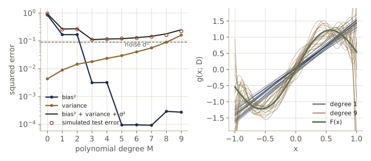
With a larger training set the variance of every model shrinks, roughly in proportion to \(1/n\), while the bias of a model that cannot represent \(F\) stays put. So the best degree grows with \(n\): more data lets us afford more flexible models. Exercise 3 asks you to check this.
Bias and variance for classification
For classification the story changes, because the loss changes. Take two categories and code the label as \(y = 1\) for \(\omega_1\) and \(y = 0\) for \(\omega_2\). The target is now the posterior
\[F(\mathbf{x}) = \Pr[y = 1 \mid \mathbf{x}] = P(\omega_1 \mid \mathbf{x}),\]and we can write \(y = F(\mathbf{x}) + \varepsilon\) with \(\varepsilon\) a zero-mean noise of variance \(F(1 - F)\), so \(F(\mathbf{x}) = \mathcal{E}[y \mid \mathbf{x}]\) and a regression method that estimates it gives a discriminant \(g(\mathbf{x}; \mathcal{D})\). But what we care about is not the squared error of \(g\); it is the 0–1 loss of the decision \(\hat{y} = 1\) if \(g > 1/2\) and \(\hat{y} = 0\) otherwise. A poor estimate of \(F\) can still give the Bayes decision, as long as it lands on the correct side of \(1/2\).
With equal priors, the Bayes decision \(y_B(\mathbf{x})\) is 1 when \(F(\mathbf{x}) > 1/2\) and 0 otherwise, and its error at \(\mathbf{x}\) is \(\min[F, 1 - F]\). For a fixed training set and a fixed \(\mathbf{x}\) there are two cases. If \(\hat{y} = y_B\), the error is \(\min[F, 1 - F]\). If \(\hat{y} \ne y_B\), the error is \(\max[F, 1 - F] = \lvert 2F - 1 \rvert + \min[F, 1 - F]\). Averaging over training sets therefore gives
Result. At every \(\mathbf{x}\),
\[\Pr[\hat{y}(\mathbf{x}; \mathcal{D}) \ne y] = \lvert 2F(\mathbf{x}) - 1 \rvert \, \Pr[\hat{y}(\mathbf{x}; \mathcal{D}) \ne y_B(\mathbf{x})] + \Pr[y_B(\mathbf{x}) \ne y].\]
The last term is the Bayes error, which no classifier can avoid. The excess error is proportional to \(\Pr[\hat{y} \ne y_B]\), the boundary error: the probability, over training sets, that the learned classifier falls on the wrong side of the Bayes boundary at \(\mathbf{x}\). It is weighted by \(\lvert 2F - 1 \rvert\), so mistakes near the Bayes boundary, where \(F\) is close to \(1/2\), cost little.
To see how bias and variance enter, suppose that over training sets \(g(\mathbf{x}; \mathcal{D})\) is roughly Gaussian with mean \(\bar{g}\) and variance \(\operatorname{Var}[g]\). If \(F > 1/2\), a boundary error happens when \(g < 1/2\), with probability \(\Phi\big((1/2 - \bar{g})/\sqrt{\operatorname{Var}[g]}\big)\), where \(\Phi\) is the standard normal distribution function; if \(F < 1/2\), it happens when \(g > 1/2\). Both cases fit into one formula:
\[\Pr[\hat{y} \ne y_B] \approx \Phi\left(-\frac{b(\mathbf{x})}{\sqrt{\operatorname{Var}[g(\mathbf{x}; \mathcal{D})]}}\right), \qquad b(\mathbf{x}) = \operatorname{sgn}\left[F(\mathbf{x}) - \tfrac{1}{2}\right]\left(\bar{g}(\mathbf{x}) - \tfrac{1}{2}\right).\](DHS write the same expression with the upper-tail function, \(1 - \Phi\), and the opposite sign.) The quantity \(b\) is the boundary bias. It is positive when the average estimate lies on the correct side of \(1/2\) and negative when it lies on the wrong side, and it measures how far from \(1/2\) the average lies.
This formula behaves very differently from the regression decomposition, where bias and variance simply add:
- When the boundary bias is positive, the error is small, and it goes to zero as the variance shrinks. The size of the bias hardly matters; an estimate that is badly biased as a probability (say \(\bar{g} = 0.9\) when \(F = 0.6\)) gives the Bayes decision anyway.
- When the boundary bias is negative, shrinking the variance makes things worse: the classifier is then reliably wrong. Here extra variance helps, because it sometimes pushes \(g\) across \(1/2\).
- Bias and variance interact multiplicatively, through the ratio \(b/\sqrt{\operatorname{Var}[g]}\), not additively.
Over most of input space a reasonable classifier’s boundary bias is positive, and there low variance is what matters. That is the sense in which, for classification, variance tends to dominate bias. It also explains why very biased classifiers, such as naive Bayes with its false independence assumption, often classify well: their probability estimates are poor, but on the right side of \(1/2\).
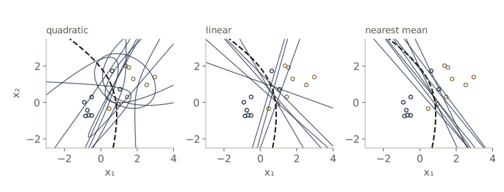
We test these claims on a two-dimensional problem with Gaussian classes of different covariances and equal priors, so the Bayes boundary is a conic. Three Gaussian classifiers are fitted by maximum likelihood with increasingly strong assumptions, as in module 03:
- quadratic: each class has its own full covariance matrix (low bias, high variance);
- linear: the classes share one pooled covariance matrix;
- nearest mean: both covariances are fixed at the identity, so only the means are estimated (high bias, low variance).
Each classifier’s discriminant \(g(\mathbf{x}; \mathcal{D})\) is its estimated posterior \(\hat{P}(\omega_1 \mid \mathbf{x})\). We draw 300 training sets with 8 samples per class, fit all three models to each, and evaluate them at 2000 test points drawn from the two classes.
from scipy.linalg import cho_factor, cho_solve

mu_c = [np.array([0.0, 0.0]), np.array([1.5, 1.0])]
Sig_c = [np.array([[1.2, 0.7], [0.7, 0.8]]), np.array([[0.6, 0.3], [0.3, 0.6]])]

def gauss_logpdf(X, mu, S):
    c = cho_factor(S, lower=True)
    diff = X - mu
    maha = np.sum(diff * cho_solve(c, diff.T).T, axis=1)
    return -0.5 * maha - np.sum(np.log(np.diag(c[0]))) - np.log(2 * np.pi)   # d = 2

def true_posterior(X):
    return expit(gauss_logpdf(X, mu_c[0], Sig_c[0]) - gauss_logpdf(X, mu_c[1], Sig_c[1]))

def sample_classes(n_per, rng):
    X = np.vstack([rng.multivariate_normal(mu_c[k], Sig_c[k], n_per) for k in (0, 1)])
    y = np.repeat([1, 0], n_per)                       # 1 = omega_1, 0 = omega_2
    return X, y

def fit_gauss(X, y, kind):
    """ML Gaussian classifier: kind is 'quadratic', 'linear', or 'nearest mean'. Equal priors."""
    mus = [X[y == 1].mean(axis=0), X[y == 0].mean(axis=0)]
    covs = [np.cov(X[y == c].T, bias=True) for c in (1, 0)]
    if kind == "linear":
        pooled = (covs[0] * np.sum(y == 1) + covs[1] * np.sum(y == 0)) / len(y)
        covs = [pooled, pooled]
    elif kind == "nearest mean":
        covs = [np.eye(2), np.eye(2)]
    return mus, covs

def gauss_posterior(model, X):
    mus, covs = model
    return expit(gauss_logpdf(X, mus[0], covs[0]) - gauss_logpdf(X, mus[1], covs[1]))

rng_cb = np.random.default_rng(55)
X_cte, _ = sample_classes(1000, rng_cb)                # 2000 test points
F_cte = true_posterior(X_cte)
yB = (F_cte > 0.5).astype(int)
bayes_err = np.mean(np.minimum(F_cte, 1 - F_cte))
kinds = ["quadratic", "linear", "nearest mean"]
R_c = 300
Gc = {k: np.empty((R_c, len(X_cte))) for k in kinds}
for r in range(R_c):
    Xtr, ytr = sample_classes(8, rng_cb)
    for k in kinds:
        Gc[k][r] = gauss_posterior(fit_gauss(Xtr, ytr, k), X_cte)

print(f"Bayes error on the test points: {bayes_err:.4f}")
print("model          error   = Bayes + |2F-1| x boundary err   boundary err  "
      "wrong-side points  Gaussian approx (corr)")
for k in kinds:
    yhat = (Gc[k] > 0.5).astype(int)
    err = np.mean(np.where(yhat == 1, 1 - F_cte, F_cte))          # exact expected error
    p_b = np.mean(yhat != yB, axis=0)                              # boundary error at each x
    decomposed = bayes_err + np.mean(np.abs(2 * F_cte - 1) * p_b)
    gbar, sd = Gc[k].mean(axis=0), Gc[k].std(axis=0) + 1e-12
    b = np.sign(F_cte - 0.5) * (gbar - 0.5)                        # boundary bias
    approx = ndtr(-b / sd)
    print(f"{k:13s} {err:.4f}   {decomposed:.4f}                      {p_b.mean():.4f}"
          f"       {np.mean(b < 0):6.3f}          {np.corrcoef(approx, p_b)[0, 1]:.3f}")
Bayes error on the test points: 0.2020
model          error   = Bayes + |2F-1| x boundary err   boundary err  wrong-side points  Gaussian approx (corr)
quadratic     0.2652   0.2652                      0.1528        0.009          0.995
linear        0.2404   0.2404                      0.1188        0.012          0.995
nearest mean  0.2160   0.2160                      0.0720        0.039          0.998
The first two columns agree to every digit, as the decomposition says they must. With only eight points per class the ranking is the reverse of the models’ flexibility. The quadratic classifier can represent the Bayes boundary, so its boundary bias is negative at fewer than 1% of the test points, yet it has the highest error (0.265 against a Bayes error of 0.202), because its boundary moves a lot from one training set to the next. The nearest-mean classifier has four times as many points with wrong-side bias, since its straight boundary cannot follow the conic, but its low variance gives it the lowest error, 0.216. The Gaussian approximation to the boundary error tracks the empirical boundary error closely (correlations above 0.99 in the last column), even though the posterior estimates are far from Gaussian near 0 and 1.
The next cell looks at the wrong-side points separately, and then repeats the comparison for larger training sets.
for k in kinds:
    yhat = (Gc[k] > 0.5).astype(int)
    p_b = np.mean(yhat != yB, axis=0)
    b = np.sign(F_cte - 0.5) * (Gc[k].mean(axis=0) - 0.5)
    print(f"{k:13s} boundary error where b > 0: {p_b[b > 0].mean():.3f};  where b < 0: "
          f"{p_b[b < 0].mean():.3f}")

print("\nexpected error by training-set size (per class):")
print("n/class  " + "  ".join(f"{k:>12s}" for k in kinds))
for n_per in (8, 30, 100, 300):
    errs = np.zeros(3)
    for r in range(100):
        Xtr, ytr = sample_classes(n_per, rng_cb)
        for i, k in enumerate(kinds):
            yhat = gauss_posterior(fit_gauss(Xtr, ytr, k), X_cte) > 0.5
            errs[i] += np.mean(np.where(yhat, 1 - F_cte, F_cte)) / 100
    print(f"{n_per:6d}   " + "  ".join(f"{e:12.4f}" for e in errs))
quadratic     boundary error where b > 0: 0.150;  where b < 0: 0.501
linear        boundary error where b > 0: 0.114;  where b < 0: 0.514
nearest mean  boundary error where b > 0: 0.050;  where b < 0: 0.623

expected error by training-set size (per class):
n/class     quadratic        linear  nearest mean
     8         0.2769        0.2464        0.2208
    30         0.2136        0.2111        0.2091
   100         0.2047        0.2054        0.2072
   300         0.2028        0.2035        0.2067
Where the boundary bias is positive, the boundary error is small, and smallest for the low-variance nearest-mean model. Where it is negative, the boundary error is above one half, because the classifier is usually on the wrong side there, and it is highest (0.62) for the nearest-mean model, whose low variance keeps it reliably wrong. As the training set grows, every model’s variance falls. The quadratic model’s error falls toward the Bayes error, since its bias is essentially zero, while the nearest-mean model levels off at an error set by its bias; by 100 points per class the ranking has flipped. The best model for a given problem depends on the amount of data, and matching the model to the truth requires prior knowledge about the form of the true distributions.
Resampling for estimating statistics
Bias and variance are defined by averages over training sets we do not have. In the simulations above we could draw as many training sets as we liked, because we knew the true distributions. With one data set in hand, can we still estimate how much a quantity computed from it would vary, and whether it is biased? Resampling methods answer yes, approximately, by treating the data set as a stand-in for the population and drawing new data sets from it.
We start with the simplest setting, a statistic of one-dimensional data, and turn to classifiers in the next section. For the sample mean we know the answer: with data \(x_1, \dots, x_n\),
\[\hat{\mu} = \frac{1}{n}\sum_{i=1}^n x_i, \qquad \widehat{\operatorname{Var}}[\hat{\mu}] = \frac{1}{n(n-1)}\sum_{i=1}^n (x_i - \hat{\mu})^2 .\]For the median, a trimmed mean, a percentile, or the mode, there is no such simple formula for the spread of the estimate. The jackknife and the bootstrap give one for any statistic.
The jackknife
Write \(\hat{\theta} = \hat{\theta}(x_1, \dots, x_n)\) for the statistic computed on all the data and
\[\hat{\theta}_{(i)} = \hat{\theta}(x_1, \dots, x_{i-1}, x_{i+1}, \dots, x_n)\]for the statistic computed with the \(i\)th point left out. The jackknife works with these \(n\) leave-one-out values and their average \(\hat{\theta}_{(\cdot)} = \frac{1}{n}\sum_i \hat{\theta}_{(i)}\).
Start with the mean to see where the formulas come from. The leave-one-out mean is \(\hat{\mu}_{(i)} = (n\hat{\mu} - x_i)/(n - 1)\), so the leave-one-out means average back to \(\hat{\mu}_{(\cdot)} = \hat{\mu}\), and each one differs from their average by \(\hat{\mu}_{(i)} - \hat{\mu}_{(\cdot)} = -(x_i - \hat{\mu})/(n - 1)\). The leave-one-out values are much less spread out than the data, by a factor of \(n - 1\), because any two of them share \(n - 2\) points. To recover the variance of \(\hat{\mu}\) from them we must scale their spread back up:
\[\frac{n-1}{n}\sum_{i=1}^n \left(\hat{\mu}_{(i)} - \hat{\mu}_{(\cdot)}\right)^2 = \frac{n-1}{n}\sum_{i=1}^n \frac{(x_i - \hat{\mu})^2}{(n-1)^2} = \frac{1}{n(n-1)}\sum_{i=1}^n (x_i - \hat{\mu})^2,\]which is exactly the classical formula. The jackknife uses the same scaled spread for any statistic.
Definition. The jackknife estimates of the variance and the bias of a statistic \(\hat{\theta}\) are
\[\operatorname{Var}_{\text{jack}}[\hat{\theta}] = \frac{n-1}{n}\sum_{i=1}^n \left(\hat{\theta}_{(i)} - \hat{\theta}_{(\cdot)}\right)^2, \qquad \text{bias}_{\text{jack}} = (n - 1)\left(\hat{\theta}_{(\cdot)} - \hat{\theta}\right),\]and the bias-corrected jackknife estimate of \(\theta\) is \(\tilde{\theta} = \hat{\theta} - \text{bias}_{\text{jack}} = n\hat{\theta} - (n - 1)\hat{\theta}_{(\cdot)}\).
Here the bias of an estimator means \(\mathcal{E}[\hat{\theta}] - \theta\), how far its average value lies from the true value. (DHS write this definition with the opposite sign, but their jackknife formulas agree with ours.) The factor \(n - 1\) in the bias formula has a clean justification. Many estimators have a bias that expands in powers of \(1/n\), say \(\mathcal{E}[\hat{\theta}_n] = \theta + a/n + b/n^2 + \cdots\). Each leave-one-out estimate uses \(n - 1\) points, so
\[\mathcal{E}\left[\hat{\theta}_{(\cdot)} - \hat{\theta}\right] = \frac{a}{n-1} - \frac{a}{n} + O\left(\frac{1}{n^2}\right) = \frac{a}{n(n-1)} + O\left(\frac{1}{n^2}\right),\]and multiplying by \(n - 1\) gives \(a/n\), the leading bias term. The corrected estimate \(\tilde{\theta}\) therefore has bias of order \(1/n^2\). When the bias is exactly \(a/n\), the correction removes it exactly. The plug-in variance \(\hat{\sigma}^2 = \frac{1}{n}\sum_i (x_i - \hat{\mu})^2\) is such a case: its expectation is \(\sigma^2 - \sigma^2/n\), and the jackknife turns it into the unbiased sample variance with divisor \(n - 1\).
We write the jackknife for statistics that work along the last axis of an array, so that all \(n\) leave-one-out samples are processed at once. The first check uses the mean and the plug-in variance, where we know the answers.
def jackknife(x, stat):
    """Jackknife: returns (theta_hat, bias_jack, var_jack, leave-one-out values)."""
    n = len(x)
    X_loo = np.broadcast_to(x, (n, n))[~np.eye(n, dtype=bool)].reshape(n, n - 1)  # row i: no x_i
    loo = stat(X_loo)
    theta, theta_dot = stat(x), loo.mean()
    bias = (n - 1) * (theta_dot - theta)
    var = (n - 1) / n * np.sum((loo - theta_dot)**2)
    return theta, bias, var, loo

def mean_stat(x):
    return x.mean(axis=-1)

def plugin_var(x):
    return x.var(axis=-1)                     # divisor n

def median_stat(x):
    return np.median(x, axis=-1)

def trimmed_mean(x, frac=0.2):
    """Drop a fraction frac at each end; if frac * n is fractional, weight the next point partially."""
    xs = np.sort(x, axis=-1)
    n = xs.shape[-1]
    r = int(frac * n)
    f = frac * n - r
    w = np.ones(n)
    w[:r], w[n - r:] = 0.0, 0.0
    w[r] -= f
    w[n - r - 1] -= f
    return xs @ w / (n * (1 - 2 * frac))

rng_s = np.random.default_rng(8)
n_s = 25
x_s = rng_s.gamma(2.0, 1.0, n_s)            # a skewed sample: Gamma with shape 2, scale 1

_, _, v_jack, _ = jackknife(x_s, mean_stat)
print(f"mean: jackknife variance {v_jack:.6f}, classical s^2/n {x_s.var(ddof=1) / n_s:.6f}")
th, b_jack, _, _ = jackknife(x_s, plugin_var)
print(f"plug-in variance {th:.4f}; jackknife-corrected {th - b_jack:.4f}; "
      f"unbiased s^2 {x_s.var(ddof=1):.4f}")
mean: jackknife variance 0.062423, classical s^2/n 0.062423
plug-in variance 1.4982; jackknife-corrected 1.5606; unbiased s^2 1.5606
Both identities hold to all printed digits.
The bootstrap
A bootstrap data set is made by drawing \(n\) points from \(\mathcal{D}\) at random with replacement, so that some points appear several times and others not at all. The bootstrap repeats this independently \(B\) times and computes the statistic on each bootstrap set, giving values \(\hat{\theta}^{*(1)}, \dots, \hat{\theta}^{*(B)}\) with average \(\hat{\theta}^{*(\cdot)}\). The estimates are
\[\text{bias}_{\text{boot}} = \hat{\theta}^{*(\cdot)} - \hat{\theta}, \qquad \operatorname{Var}_{\text{boot}}[\hat{\theta}] = \frac{1}{B}\sum_{b=1}^B \left(\hat{\theta}^{*(b)} - \hat{\theta}^{*(\cdot)}\right)^2 .\]The idea is a substitution. The unknown population generates data sets, and the statistic varies around the true \(\theta\). The data set’s own empirical distribution (probability \(1/n\) on each observed point) generates bootstrap sets, and the statistic varies around \(\hat{\theta}\), the value of the statistic for that empirical distribution. If the empirical distribution resembles the population, the bootstrap variation resembles the true sampling variation. For the mean, the bootstrap variance tends, as \(B \to \infty\), to \(\hat{\sigma}^2/n\) with the plug-in \(\hat{\sigma}^2\) (Exercise 5). For the plug-in variance itself the bootstrap bias estimate tends to \(-\hat{\sigma}^2/n\), the plug-in version of the true bias \(-\sigma^2/n\).
The jackknife always needs exactly \(n\) recomputations. The bootstrap lets us choose \(B\) to suit the computing budget: more resamples give a less noisy estimate, and a few hundred usually suffice for a variance, more for the tails of the distribution.
def bootstrap(x, stat, B, rng):
    """Bootstrap: returns (bias_boot, var_boot, replicates)."""
    idx = rng.integers(0, len(x), size=(B, len(x)))
    reps = stat(x[idx])
    return reps.mean() - stat(x), reps.var(), reps

b_boot, v_boot, _ = bootstrap(x_s, mean_stat, 200_000, np.random.default_rng(1))
print(f"mean: bootstrap variance {v_boot:.6f}, plug-in sigma^2/n {x_s.var() / n_s:.6f}")
b_boot, _, _ = bootstrap(x_s, plugin_var, 200_000, np.random.default_rng(2))
print(f"plug-in variance: bootstrap bias {b_boot:.4f}, -sigma_hat^2/n {-x_s.var() / n_s:.4f}")
mean: bootstrap variance 0.059651, plug-in sigma^2/n 0.059926
plug-in variance: bootstrap bias -0.0604, -sigma_hat^2/n -0.0599
Checking against the truth
Now the real test: statistics without simple formulas, on data where we know the truth. The population is the gamma distribution with shape 2 and scale 1, whose median and 20%-trimmed mean we can compute from the incomplete gamma function. (The 20%-trimmed mean drops the lowest and highest 20% of the sorted data and averages the rest. When 20% of \(n\) is not a whole number, as for the leave-one-out sets of size 24, our version gives the last point kept at each end a partial weight, so that the statistic always trims exactly 20%. With whole-point trimming the leave-one-out sets would trim a different fraction, and the jackknife would mistake that difference for bias.) By drawing 20,000 data sets of size 25 from the population we get Monte Carlo values for the true standard error and bias of each statistic. Then we compare the jackknife and bootstrap estimates computed from our one data set.
from scipy.special import gammainc, gammaincinv

# population values for Gamma(shape 2, scale 1)
med_pop = gammaincinv(2.0, 0.5)
q_lo, q_hi = gammaincinv(2.0, 0.2), gammaincinv(2.0, 0.8)
trim_pop = 2.0 * (gammainc(3.0, q_hi) - gammainc(3.0, q_lo)) / 0.6   # E[X; q_lo < X < q_hi]/0.6

X_mc = np.random.default_rng(77).gamma(2.0, 1.0, size=(20_000, n_s))
stats = {"median": (median_stat, med_pop), "20% trimmed mean": (trimmed_mean, trim_pop)}
rng_b = np.random.default_rng(5)
print("statistic          estimate   SE: jack   boot    true   bias: jack    boot    true")
for name, (stat, pop) in stats.items():
    th, b_j, v_j, _ = jackknife(x_s, stat)
    b_b, v_b, _ = bootstrap(x_s, stat, 2000, rng_b)
    mc = stat(X_mc)
    print(f"{name:18s} {th:8.4f}   {np.sqrt(v_j):8.4f} {np.sqrt(v_b):6.4f} {mc.std():7.4f}"
          f"   {b_j:9.4f} {b_b:7.4f} {mc.mean() - pop:7.4f}")
statistic          estimate   SE: jack   boot    true   bias: jack    boot    true
median               1.0828     0.6235 0.3572  0.3195      1.6584  0.0969  0.0154
20% trimmed mean     1.2662     0.3213 0.2878  0.2778      0.0261  0.0197  0.0153
For our data set, the bootstrap standard errors (0.357 and 0.288) are close to the true ones (0.320 and 0.278). The jackknife agrees for the trimmed mean but gives 0.62 for the median, nearly twice the truth, and its bias estimate for the median, 1.66, is absurd next to the true bias of 0.015. For the trimmed mean all three bias values are small, around 0.02. One data set is only one draw, though; to see how the estimators behave in general we repeat the comparison on 200 independent data sets and summarize each standard-error estimate by its average and its spread relative to the truth.
rng_rep = np.random.default_rng(6)
print("statistic          method     mean SE / true SE   spread (sd / true SE)")
for name, (stat, pop) in stats.items():
    true_se = stat(X_mc).std()
    se = {"jackknife": [], "bootstrap": []}
    for _ in range(200):
        x = rng_rep.gamma(2.0, 1.0, n_s)
        se["jackknife"].append(np.sqrt(jackknife(x, stat)[2]))
        se["bootstrap"].append(np.sqrt(bootstrap(x, stat, 500, rng_rep)[1]))
    for meth, v in se.items():
        v = np.array(v)
        print(f"{name:18s} {meth:10s} {v.mean() / true_se:12.3f} {v.std() / true_se:18.3f}")
statistic          method     mean SE / true SE   spread (sd / true SE)
median             jackknife         0.951              0.628
median             bootstrap         1.031              0.324
20% trimmed mean   jackknife         0.993              0.259
20% trimmed mean   bootstrap         1.008              0.244
For the trimmed mean both methods are nearly unbiased and about equally variable. For the median the jackknife is right on average but erratic: its standard-error estimates spread about twice as widely as the bootstrap’s. The reason is visible in the leave-one-out values. With \(n = 25\), deleting any point below the median gives one value, deleting any point above it gives another, and deleting the median itself gives a third, so the \(\hat{\theta}_{(i)}\) take only three distinct values, and the jackknife’s answer depends on just the three data points nearest the middle and on the gaps between them. The jackknife works well for smooth statistics, which change a little when one point changes a little; the median is not smooth in this sense. (DHS’s Example 2 applies the jackknife to the mode, which is even less smooth.)
_, _, _, loo_med = jackknife(x_s, median_stat)
print("distinct leave-one-out medians:", np.unique(loo_med))
distinct leave-one-out medians: [1.02 1.2157 1.2785]
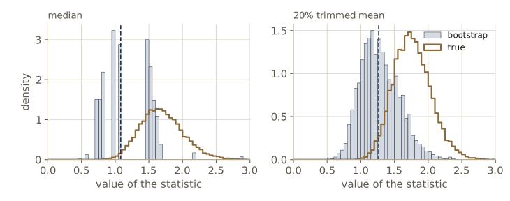
In practice. Use the bootstrap as the default for standard errors and bias of complicated statistics; use a few hundred resamples for a standard error and a few thousand for percentile-based confidence intervals. The jackknife is cheaper for smooth statistics and deterministic (no resampling noise), but it can fail for non-smooth ones such as the median and other quantiles.
Resampling for classifier design
The jackknife and bootstrap estimate properties of a statistic that has already been computed. The same idea, reusing or reweighting the training data, can also be used to build classifiers. The generic name for such methods is arcing, for “adaptive reweighting and combining”: we train several component classifiers on different versions of the training data and let them vote. This section covers bagging, boosting, and learning with queries, and then asks why training on a distribution that differs from the true one can help.
A problem with a known Bayes rule
To measure what these methods do to bias and variance we need a problem whose posterior we know. Inputs are uniform on the square \([-2, 2]^2\), and the posterior is
\[F(\mathbf{x}) = P(\omega_1 \mid \mathbf{x}) = \sigma\big(4(x_2 - \sin 1.5x_1)\big), \qquad \sigma(a) = \frac{1}{1 + e^{-a}},\]so the Bayes boundary is the wave \(x_2 = \sin 1.5x_1\), and points near it have truly uncertain labels. Since we know \(F\), we can compute the exact expected error of any classifier by averaging \(1 - F\) over the points it assigns to \(\omega_1\) and \(F\) over the others, here on a fixed set of 4000 uniformly spread points. Labels are coded \(y = 1\) for \(\omega_1\) and \(y = 0\) for \(\omega_2\).
def F_wave(X):
    return expit(4.0 * (X[:, 1] - np.sin(1.5 * X[:, 0])))

def sample_wave(n, rng):
    X = rng.uniform(-2, 2, (n, 2))
    y = (rng.uniform(0, 1, n) < F_wave(X)).astype(int)
    return X, y

X_eval = np.random.default_rng(1).uniform(-2, 2, (4000, 2))
F_eval = F_wave(X_eval)
yB_eval = (F_eval > 0.5).astype(int)

def expected_error(pred):
    """Exact expected error of 0/1 predictions at X_eval, averaged over input space."""
    return np.mean(np.where(pred == 1, 1 - F_eval, F_eval))

print(f"Bayes error: {expected_error(yB_eval):.4f}")
Bayes error: 0.0856
Decision trees and instability
Our component classifiers are the binary decision trees of module 08, grown greedily with the Gini impurity and optional sample weights. At each node we try every threshold on every feature: after sorting the node’s points along a feature, cumulative sums give the weighted class counts on each side of every candidate threshold at once.
def best_split(X, y, w):
    """Best (feature, threshold) by weighted Gini impurity; None if no split is possible."""
    best, best_imp = None, np.inf
    for j in range(X.shape[1]):
        o = np.argsort(X[:, j])
        xs, ys, ws = X[o, j], y[o], w[o]
        wl = np.cumsum(ws)[:-1]                   # weight left of each gap
        wl1 = np.cumsum(ws * ys)[:-1]             # ... of which class omega_1
        wr, wr1 = ws.sum() - wl, np.sum(ws * ys) - wl1
        pl, pr = wl1 / wl, wr1 / wr
        imp = wl * 2 * pl * (1 - pl) + wr * 2 * pr * (1 - pr)
        imp[xs[1:] == xs[:-1]] = np.inf           # only split between distinct values
        k = np.argmin(imp)
        if imp[k] < best_imp:
            best, best_imp = (j, 0.5 * (xs[k] + xs[k + 1])), imp[k]
    return best

def fit_tree(X, y, depth, w=None):
    """Tree as nested tuples: ('leaf', P(omega_1)) or ('node', j, threshold, left, right)."""
    w = np.ones(len(y)) if w is None else w
    p = np.sum(w * y) / np.sum(w)
    split = best_split(X, y, w) if depth > 0 and 0 < p < 1 and len(y) > 1 else None
    if split is None:
        return ("leaf", p)
    j, thr = split
    L = X[:, j] <= thr
    return ("node", j, thr, fit_tree(X[L], y[L], depth - 1, w[L]),
            fit_tree(X[~L], y[~L], depth - 1, w[~L]))

def tree_prob(node, X):
    if node[0] == "leaf":
        return np.full(len(X), node[1])
    _, j, thr, left, right = node
    out, L = np.empty(len(X)), X[:, j] <= thr
    out[L], out[~L] = tree_prob(left, X[L]), tree_prob(right, X[~L])
    return out

rng_t = np.random.default_rng(21)
X_w, y_w = sample_wave(200, rng_t)
for depth in (1, 3, 5, 12):
    tr = fit_tree(X_w, y_w, depth)
    train_err = np.mean((tree_prob(tr, X_w) > 0.5) != y_w)
    print(f"depth {depth:2d}: training error {train_err:.3f}, "
          f"expected test error {expected_error(tree_prob(tr, X_eval) > 0.5):.4f}")

# instability: two trees grown on two bootstrap samples of the same data
i1, i2 = rng_t.integers(0, 200, 200), rng_t.integers(0, 200, 200)
p1 = tree_prob(fit_tree(X_w[i1], y_w[i1], 12), X_eval) > 0.5
p2 = tree_prob(fit_tree(X_w[i2], y_w[i2], 12), X_eval) > 0.5
print(f"two full trees from bootstrap samples disagree on {np.mean(p1 != p2):.1%} of inputs")
depth  1: training error 0.150, expected test error 0.1760
depth  3: training error 0.045, expected test error 0.1230
depth  5: training error 0.010, expected test error 0.1295
depth 12: training error 0.000, expected test error 0.1320
two full trees from bootstrap samples disagree on 12.0% of inputs
A full-depth tree fits the training data perfectly and has a higher test error than a moderate one. It is also unstable: a small change in the training set, here a different bootstrap sample of the same 200 points, changes a large fraction of its decisions. Informally, a learning algorithm is unstable when small changes in the training data produce large changes in the classifier and its accuracy. Unstable algorithms are high-variance algorithms, and they are the ones resampling can help most.
Bagging
Bagging, short for “bootstrap aggregation”, trains each component classifier on its own bootstrap sample of the training set and classifies by a plain majority vote of the components. Averaging over many bootstrap samples smooths out the arbitrary choices that make each component unstable, which lowers the variance while leaving the bias about where it was. There is no guarantee that bagging helps every unstable classifier, but it usually helps trees, and it rarely hurts much.
def bagged_trees(X, y, B, depth, rng):
    trees = []
    for _ in range(B):
        i = rng.integers(0, len(y), len(y))      # a bootstrap sample
        trees.append(fit_tree(X[i], y[i], depth))
    return trees

def vote(trees, X):
    """Fraction of components voting for omega_1."""
    return np.mean([tree_prob(t, X) > 0.5 for t in trees], axis=0)

rng_bag = np.random.default_rng(22)
trees = bagged_trees(X_w, y_w, 100, 12, rng_bag)
single = expected_error(tree_prob(fit_tree(X_w, y_w, 12), X_eval) > 0.5)
print(f"single full tree: {single:.4f}")
for B in (1, 5, 25, 100):
    print(f"bagged, B = {B:3d}: {expected_error(vote(trees[:B], X_eval) > 0.5):.4f}")
single full tree: 0.1320
bagged, B =   1: 0.1509
bagged, B =   5: 0.1185
bagged, B =  25: 0.1206
bagged, B = 100: 0.1140
A single tree grown on one bootstrap sample (the \(B = 1\) row) is worse than the tree grown on all the data, since it sees only about 63% of the distinct points, but voting over many such trees brings the error from 0.132 down to 0.114. We measure its bias and variance directly at the end of this section. Bagging is our first multiclassifier system, and its combination rule, an unweighted vote, is the simplest of the rules we meet in the last section of this module. Intro to ML, module 14 shows why averaging \(M\) committee members can cut the expected squared error by up to a factor of \(M\) when their errors are uncorrelated, and why in practice the reduction is much smaller.
Boosting with three components
Boosting takes a different route. Instead of independent resamples, each new component is trained on data chosen to be informative given the components we already have. It starts from a weak learner, an algorithm whose accuracy is only somewhat better than chance, and combines its outputs into a classifier with arbitrarily high accuracy on the training set.
The original scheme builds three components for a two-category problem:
- Train \(C_1\) on a random subset \(\mathcal{D}_1\) of about \(n/3\) training patterns.
- Build \(\mathcal{D}_2\) so that \(C_1\) gets half of it right and half wrong: repeatedly flip a fair coin; on heads, walk through the unused patterns until \(C_1\) misclassifies one and add it; on tails, add the next one \(C_1\) classifies correctly. Stop when no pattern of the required kind is left. Train \(C_2\) on \(\mathcal{D}_2\).
- Let \(\mathcal{D}_3\) be the remaining patterns on which \(C_1\) and \(C_2\) disagree, and train \(C_3\) on them.
To classify, use the common label if \(C_1\) and \(C_2\) agree and the label of \(C_3\) otherwise, which is a majority vote of the three. The size of \(\mathcal{D}_1\) needs tuning: if \(C_1\) is very good, few of its mistakes remain for \(\mathcal{D}_2\); if it is poor, \(\mathcal{D}_2\) can become too large.
A vote of three weak components can represent decision regions that none of them can alone. With decision stumps (trees of depth one, which cut on a single feature) as the weak learner, no single stump can carve out a corner such as \(x_1 > 0,\ x_2 > 0\); but if \(C_1\) cuts on \(x_1\) and \(C_2\) on \(x_2\), they disagree exactly on the two regions next to the corner, and a \(C_3\) that says \(\omega_2\) there turns the vote into the AND of the two cuts. Whether the scheme finds such components depends on the small, oddly chosen samples each one sees, so its gains in practice tend to be modest and erratic (Exercise 8 asks you to try it). It can be applied recursively to the components, giving 9 or 27 of them and a lower training error, but the bookkeeping is awkward and each level still has only three voters. AdaBoost removes both problems.
AdaBoost
AdaBoost (“adaptive boosting”) keeps a weight \(W_k(i)\) on every training pattern and adds components one at a time for as long as we like. Patterns the current component gets wrong have their weights increased, so the next component concentrates on them. With labels \(y_i \in \{-1, +1\}\), it runs as follows.
- Start with uniform weights, \(W_1(i) = 1/n\).
- For \(k = 1, \dots, k_{\max}\):
- train the weak learner \(C_k\) on \(\mathcal{D}\) weighted by \(W_k\) (or on a sample drawn according to \(W_k\)), giving \(h_k(\mathbf{x}) \in \{-1, +1\}\);
- compute its weighted training error \(E_k = \sum_i W_k(i)\,[h_k(\mathbf{x}^i) \ne y_i]\);
- set \(\alpha_k = \frac{1}{2}\ln\frac{1 - E_k}{E_k}\);
- update \(W_{k+1}(i) = W_k(i)\,e^{-\alpha_k y_i h_k(\mathbf{x}^i)}/Z_k\), where \(Z_k\) makes the weights sum to one. This multiplies a correctly classified pattern’s weight by \(e^{-\alpha_k}\) and a misclassified pattern’s by \(e^{\alpha_k}\).
- Classify with the sign of \(g(\mathbf{x}) = \sum_{k=1}^{k_{\max}} \alpha_k h_k(\mathbf{x})\).
The component weight \(\alpha_k\) is positive whenever \(E_k < 1/2\) and grows as \(E_k\) shrinks, so better components get more say.
The training error bound. Why does the ensemble’s training error fall? Unroll the weight update: starting from \(1/n\) and multiplying by \(e^{-\alpha_k y_i h_k(\mathbf{x}^i)}/Z_k\) at each step gives
\[W_{k_{\max}+1}(i) = \frac{1}{n}\,\frac{e^{-y_i g(\mathbf{x}^i)}}{\prod_k Z_k}.\]These weights sum to one, so \(\frac{1}{n}\sum_i e^{-y_i g(\mathbf{x}^i)} = \prod_k Z_k\). A misclassified pattern has \(y_i g(\mathbf{x}^i) \le 0\) and hence \(e^{-y_i g(\mathbf{x}^i)} \ge 1\), so the training error of the ensemble is at most \(\prod_k Z_k\). Finally, compute \(Z_k\): the correctly classified patterns carry total weight \(1 - E_k\) and the others \(E_k\), so
\[Z_k = (1 - E_k)e^{-\alpha_k} + E_k e^{\alpha_k} = 2\sqrt{E_k(1 - E_k)},\]using \(e^{\alpha_k} = \sqrt{(1 - E_k)/E_k}\). (This \(\alpha_k\) is in fact the value that minimizes \(Z_k\).) Writing \(E_k = 1/2 - G_k\), where \(G_k > 0\) is how much better than chance the \(k\)th component is:
Result. The training error of the AdaBoost ensemble satisfies
\[E \le \prod_{k=1}^{k_{\max}} 2\sqrt{E_k(1 - E_k)} = \prod_{k=1}^{k_{\max}} \sqrt{1 - 4G_k^2} \le \exp\left(-2\sum_{k=1}^{k_{\max}} G_k^2\right).\]
The last step uses \(1 - u \le e^{-u}\). As long as every component is better than chance by some fixed margin, the training error falls exponentially in the number of components. (DHS state the product as an equality; it is an upper bound.)
Our weak learner is the decision stump, fitted to weighted data. For each feature we sort the points, and cumulative sums of the weights give the weighted error of every threshold and both orientations at once. The check compares it with a brute-force search on random weights.
def fit_stump(X, t, w):
    """Weighted decision stump for t in {-1, +1}: h(x) = s if x_j > theta else -s.
    Returns (j, theta, s, weighted error)."""
    best = (0, -np.inf, 1, np.inf)
    for j in range(X.shape[1]):
        o = np.argsort(X[:, j])
        xs, ts, ws = X[o, j], t[o], w[o]
        thr = np.r_[xs[0] - 1.0, 0.5 * (xs[1:] + xs[:-1])]    # threshold k has k points below it
        pos_below = np.r_[0.0, np.cumsum(ws * (ts > 0))[:-1]]
        neg_below = np.r_[0.0, np.cumsum(ws * (ts < 0))[:-1]]
        err_plus = pos_below + (np.sum(ws * (ts < 0)) - neg_below)   # s = +1: below -> -1
        errs = np.stack([err_plus, ws.sum() - err_plus])             # rows: s = +1, s = -1
        errs[:, np.r_[False, xs[1:] == xs[:-1]]] = np.inf
        s_i, k = np.unravel_index(np.argmin(errs), errs.shape)
        if errs[s_i, k] < best[3]:
            best = (j, thr[k], 1 - 2 * s_i, errs[s_i, k])
    return best

def stump_predict(stump, X):
    j, thr, s, _ = stump
    return np.where(X[:, j] > thr, s, -s)

t_w = 2 * y_w - 1
w_rand = np.random.default_rng(23).dirichlet(np.ones(len(t_w)))
st = fit_stump(X_w, t_w, w_rand)
brute = min(np.sum(w_rand * (np.where(X_w[:, j] > th, s, -s) != t_w))
            for j in range(2) for th in np.r_[X_w[:, j] - 1e-9, X_w[:, j].max() + 1] for s in (1, -1))
print(f"stump: feature {st[0]}, threshold {st[1]:.3f}, sign {st[2]:+d}, weighted error {st[3]:.4f};"
      f"  brute force {brute:.4f}")
stump: feature 1, threshold 0.047, sign +1, weighted error 0.1199; brute force 0.1199
def adaboost(X, t, k_max, X_test=None):
    n = len(t)
    W = np.full(n, 1.0 / n)
    g_train = np.zeros(n)
    g_test = None if X_test is None else np.zeros(len(X_test))
    stumps, alphas, hist = [], [], []
    for k in range(k_max):
        st = fit_stump(X, t, W)
        E_k = st[3]
        alpha = 0.5 * np.log((1 - E_k) / E_k)
        h = stump_predict(st, X)
        W = W * np.exp(-alpha * t * h)
        W /= W.sum()                                   # divide by Z_k
        g_train += alpha * h
        stumps.append(st)
        alphas.append(alpha)
        row = [E_k, np.mean(np.sign(g_train) != t)]
        if X_test is not None:
            g_test += alpha * stump_predict(st, X_test)
            row.append(expected_error((g_test > 0).astype(int)))
        hist.append(row)
    return stumps, np.array(alphas), np.array(hist)

rng_ab = np.random.default_rng(24)
X_ab, y_ab = sample_wave(300, rng_ab)
t_ab = 2 * y_ab - 1
stumps_ab, alphas_ab, hist_ab = adaboost(X_ab, t_ab, 400, X_eval)
E_k = hist_ab[:, 0]
bound = np.cumprod(2 * np.sqrt(E_k * (1 - E_k)))
exp_bound = np.exp(-2 * np.cumsum((0.5 - E_k)**2))
print(" k    E_k    train error   product bound   exp bound   test error")
for k in (1, 2, 5, 10, 20, 50, 100, 200, 400):
    print(f"{k:3d}  {E_k[k - 1]:.3f}     {hist_ab[k - 1, 1]:.3f}        {bound[k - 1]:.3f}"
          f"         {exp_bound[k - 1]:.3f}      {hist_ab[k - 1, 2]:.4f}")
print("bound holds at every round:", bool(np.all(hist_ab[:, 1] <= bound + 1e-12)))
 k    E_k    train error   product bound   exp bound   test error
  1  0.183     0.183        0.774         0.818      0.1960
  2  0.234     0.183        0.656         0.711      0.1960
  5  0.372     0.117        0.478         0.539      0.1125
 10  0.380     0.093        0.402         0.456      0.1036
 20  0.424     0.077        0.354         0.402      0.0928
 50  0.444     0.073        0.287         0.327      0.0958
100  0.457     0.060        0.240         0.274      0.0986
200  0.467     0.037        0.186         0.213      0.1040
400  0.469     0.013        0.123         0.141      0.1114
bound holds at every round: True
The weighted error of each new stump rises toward one half as the weights concentrate on the hard patterns near the wave, yet the ensemble’s training error keeps falling, always below the product bound (which is loose, but falls steadily). The test error drops from 0.196 for one stump to about 0.093 after 20 rounds, not far above the Bayes error of 0.086. After that it creeps up, to 0.111 at round 400, while the training error falls far below the Bayes error: with labels this noisy, boosting does overfit, though slowly. On problems with less label noise, the test error of boosting often keeps improving long after the training error reaches zero, which is why DHS remark that running beyond the point of zero training error can help. The number of rounds is a complexity parameter, and cross-validation, later in this module, is the usual way to set it.
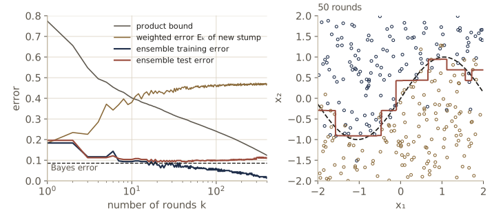
Does boosting contradict the no free lunch theorem, since the training error always falls? No. The guarantee requires every component to beat chance on its weighted data, which nothing ensures in advance; if the weak learner cannot do that on a problem, boosting has nothing to work with. And a low training error says nothing about off-training-set error without assumptions about the target. Intro to ML, module 14 derives AdaBoost as the stagewise minimization of the exponential error \(\sum_i e^{-y_i g(\mathbf{x}^i)}\), which is exactly the quantity we bounded above.
Learning with queries
So far the labeled training set was fixed. In many applications unlabeled patterns are cheap and labels are expensive: every label requires a person to look at a scanned document, a medical image, or a recording. Then it pays to choose which patterns to label. In learning with queries (also active learning) the classifier selects an unlabeled pattern, sends it as a query to an oracle, a teacher that can label any pattern without error, adds the answer to its training set, and repeats. When labels have different costs, cost-based learning trades classifier accuracy against the cost of the labels.
Which patterns are most informative? Usually those the current classifier is least sure about, which lie near its current decision boundary. Two common rules:
- confidence-based query selection: query the pattern for which the two largest discriminant functions \(g_i(\mathbf{x})\) are closest; for a two-category posterior estimate, the pattern with \(\hat{P}(\omega_1 \mid \mathbf{x})\) closest to \(1/2\) (also called uncertainty sampling);
- voting-based (or committee-based) query selection: train several component classifiers and query the pattern on which their votes are most evenly split. This works even for classifiers without analog outputs, such as trees, rule sets, or \(k\)-nearest-neighbor rules.
We compare confidence-based selection with random selection on two well-separated Gaussian classes (identity covariances, Bayes error about 0.04), using logistic regression with a small ridge penalty so that it stays finite on separable data, fitted by Newton’s method as in module 05. Each run starts from two labeled points per class and a pool of 1000 unlabeled points. For a linear rule \(\mathbf{w}^{t}\mathbf{x} + w_0 > 0 \Rightarrow \omega_1\) and Gaussian classes with identity covariance, the exact error is an average of two normal tail probabilities, so we need no test set.
mu_q = [np.array([0.0, 0.0]), np.array([2.5, 2.5])]

def fit_logistic(X, y, lam=0.01, iters=30):
    """Ridge-penalized logistic regression by Newton's method; returns a = (w0, w)."""
    Y = np.column_stack([np.ones(len(X)), X])
    a = np.zeros(Y.shape[1])
    for _ in range(iters):
        p = expit(Y @ a)
        grad = Y.T @ (p - y) + lam * a
        H = (Y * (p * (1 - p))[:, None]).T @ Y + lam * np.eye(len(a))
        a -= np.linalg.solve(H, grad)
    return a

def linear_rule_error(a):
    """Exact error of 'omega_1 if w.x + w0 > 0' for N(mu_q[0], I) vs N(mu_q[1], I)."""
    w0, w = a[0], a[1:]
    s = np.linalg.norm(w)
    return 0.5 * ndtr(-(w @ mu_q[0] + w0) / s) + 0.5 * ndtr((w @ mu_q[1] + w0) / s)

def active_run(strategy, budget, rng):
    pool = np.vstack([rng.normal(mu_q[0], 1.0, (500, 2)), rng.normal(mu_q[1], 1.0, (500, 2))])
    labels = np.repeat([1, 0], 500)                  # the oracle's answers
    chosen = (list(rng.choice(500, 2, replace=False))
              + list(500 + rng.choice(500, 2, replace=False)))
    errors = {}
    while len(chosen) <= budget:
        a = fit_logistic(pool[chosen], labels[chosen])
        errors[len(chosen)] = linear_rule_error(a)
        free = np.setdiff1d(np.arange(1000), chosen)
        if strategy == "confidence":
            p = expit(a[0] + pool[free] @ a[1:])
            chosen.append(free[np.argmin(np.abs(p - 0.5))])
        else:
            chosen.append(rng.choice(free))
    return errors

bayes_q = ndtr(-np.linalg.norm(mu_q[1] - mu_q[0]) / 2)
rng_al = np.random.default_rng(25)
runs = {s: [active_run(s, 40, rng_al) for _ in range(30)] for s in ("random", "confidence")}
print(f"Bayes error {bayes_q:.4f}; mean error over 30 runs:")
print("labels   random   confidence")
for m in (4, 6, 10, 20, 40):
    print(f"{m:5d}   {np.mean([r[m] for r in runs['random']]):.4f}     "
          f"{np.mean([r[m] for r in runs['confidence']]):.4f}")
Bayes error 0.0385; mean error over 30 runs:
labels   random   confidence
    4   0.1051     0.1172
    6   0.0964     0.0756
   10   0.0815     0.0519
   20   0.0635     0.0433
   40   0.0519     0.0405
With only the four starting labels the two strategies are the same up to chance. After that, queries chosen near the boundary improve the classifier much faster: with 10 labels the active learner’s error is 0.052 against 0.082 for random labels, and with 20 labels it is at 0.043, better than the random learner with 40 labels and close to the Bayes error of 0.039. The queried points pile up near the decision boundary rather than where the data are dense. When no pool of unlabeled data is available, queries can sometimes be synthesized instead, for example by distorting or interpolating labeled patterns in a way that suits the domain.
Arcing, learning with queries, bias, and variance
Earlier modules insisted that a classifier be trained on data drawn from the distribution it will face. Bagging, boosting, and queries all break that rule: boosting’s weights and active learning’s queries produce training sets heavily concentrated near the decision boundary. Why does this help rather than hurt?
Two reasons. First, these methods are normally used with classifiers that do not try to model the class-conditional densities. Trees, stumps, nearest-neighbor rules, and logistic regression aim at the decision boundary directly, and for them the most useful data are near the boundary. Fitting a density model to a skewed sample would indeed go wrong: a Gaussian fitted by maximum likelihood to boundary-hugging queries would get the class means and covariances badly wrong. Second, combining many components enlarges the family of decision functions: a single stump has an axis-parallel boundary, while a weighted vote of stumps can follow the wave. Resampling methods are therefore ways of adjusting the effective complexity of a classifier, and with it the bias and variance, for any base learner, including ones such as multilayer networks whose complexity is otherwise hard to tune.
We can measure this with the classification version of bias and variance. Train each method on 20 independent training sets of 200 points. At each evaluation point, the method’s main prediction is the label most of the 20 classifiers give; its bias is whether the main prediction differs from the Bayes decision, and its variance is the fraction of the 20 classifiers that disagree with the main prediction.
def bias_variance_classifier(fit_predict, R=20, n=200, seed=26):
    rng_bv2 = np.random.default_rng(seed)
    P = np.array([fit_predict(*sample_wave(n, rng_bv2), rng_bv2) for _ in range(R)])
    main = (P.mean(axis=0) > 0.5).astype(int)
    bias = np.mean(main != yB_eval)
    var = np.mean(P != main)
    err = np.mean([expected_error(p) for p in P])
    return bias, var, err

def fp_stump(X, y, rng_):
    return (stump_predict(fit_stump(X, 2 * y - 1, np.ones(len(y))), X_eval) > 0).astype(int)

def fp_boost(X, y, rng_):
    st, al, _ = adaboost(X, 2 * y - 1, 100)
    return (sum(a * stump_predict(s, X_eval) for s, a in zip(st, al)) > 0).astype(int)

def fp_tree(X, y, rng_):
    return (tree_prob(fit_tree(X, y, 12), X_eval) > 0.5).astype(int)

def fp_bagged(X, y, rng_):
    return (vote(bagged_trees(X, y, 25, 12, rng_), X_eval) > 0.5).astype(int)

print("method                   bias   variance   expected error")
for name, fp in [("single stump", fp_stump), ("AdaBoost, 100 stumps", fp_boost),
                 ("full tree", fp_tree), ("bagged trees, B = 25", fp_bagged)]:
    b, v, e = bias_variance_classifier(fp)
    print(f"{name:22s}  {b:.3f}     {v:.3f}        {e:.4f}")
method                   bias   variance   expected error
single stump            0.159     0.052        0.1806
AdaBoost, 100 stumps    0.023     0.059        0.1067
full tree               0.029     0.090        0.1295
bagged trees, B = 25    0.026     0.065        0.1118
The single stump has large bias and small variance: its one straight cut cannot follow the wave, but it is always roughly the same cut. Boosting cuts its bias sharply, at the cost of some variance. The full tree has the opposite profile, small bias and large variance, and bagging leaves its bias about the same while removing much of its variance. So, in rough terms, bagging is a variance-reduction method, boosting mainly reduces bias, and which one helps depends on which of the two limits the base learner. These 0–1 bias and variance numbers are not additive like the regression terms; they are descriptive summaries, not an exact decomposition of the error.
Estimating and comparing classifiers
We want to know a classifier’s generalization error for two reasons: to decide whether it is good enough to use, and to decide whether it is better than a competitor. Every method for estimating it rests on assumptions, sometimes explicit (a parametric model), more often implicit, and every one can fail when its assumptions do. That is unavoidable: a method that always picked the better of two classifiers on a new problem could be built into a learning algorithm that beats all others, contradicting the no free lunch theorem. So the methods in this section are heuristics, and good ones.
Parametric models
If we trust a parametric model, we can compute the error from it. For two Gaussian classes with a shared covariance and equal priors, the Bayes error is \(\Phi(-\Delta/2)\), where \(\Delta\) is the Mahalanobis distance between the means (module 02); for more complicated models the Chernoff and Bhattacharyya bounds give upper bounds. Plugging in estimated parameters gives an estimate of the error. This has three problems. It tends to be optimistic, because whatever makes the training sample peculiar also shapes the estimate. It inherits any error in the model, so an estimate from a doubtful model can only be believed when it is unfavorable. And for realistic models the error cannot be computed in closed form anyway.
The optimism is easy to see. We draw 15 samples per class from two five-dimensional Gaussians with a shared covariance, fit the linear classifier of module 02 with plug-in means and pooled covariance, and compare the plug-in error \(\Phi(-\hat{\Delta}/2)\) with the true error of the fitted classifier, which we can compute exactly because the classes are Gaussian.
d_p, n_p = 5, 15
mu_p = [np.zeros(d_p), np.r_[1.0, 0.8, 0.0, 0.0, 0.0]]
A_p = np.random.default_rng(40).normal(size=(d_p, d_p))
Sig_p = A_p @ A_p.T / d_p + 0.5 * np.eye(d_p)
L_p = np.linalg.cholesky(Sig_p)
delta_true = np.sqrt((mu_p[1] - mu_p[0]) @ np.linalg.solve(Sig_p, mu_p[1] - mu_p[0]))

def linear_error_exact(w, w0):
    """True error of 'omega_1 if w.x + w0 > 0' for N(mu_p[0], Sig_p) vs N(mu_p[1], Sig_p)."""
    s = np.sqrt(w @ Sig_p @ w)
    return 0.5 * ndtr(-(w @ mu_p[0] + w0) / s) + 0.5 * ndtr((w @ mu_p[1] + w0) / s)

rng_p = np.random.default_rng(41)
plug, true, resub = [], [], []
for _ in range(500):
    X1 = mu_p[0] + rng_p.standard_normal((n_p, d_p)) @ L_p.T
    X2 = mu_p[1] + rng_p.standard_normal((n_p, d_p)) @ L_p.T
    m1, m2 = X1.mean(axis=0), X2.mean(axis=0)
    S = (np.cov(X1.T) + np.cov(X2.T)) / 2               # pooled, unbiased
    w = np.linalg.solve(S, m1 - m2)
    w0 = -0.5 * w @ (m1 + m2)
    plug.append(ndtr(-np.sqrt((m1 - m2) @ w) / 2))
    true.append(linear_error_exact(w, w0))
    resub.append(0.5 * np.mean(X1 @ w + w0 <= 0) + 0.5 * np.mean(X2 @ w + w0 > 0))
print(f"Bayes error {ndtr(-delta_true / 2):.4f}")
print(f"average plug-in estimate {np.mean(plug):.4f}, average resubstitution error "
      f"{np.mean(resub):.4f}, average true error {np.mean(true):.4f}")
Bayes error 0.2825
average plug-in estimate 0.2269, average resubstitution error 0.2229, average true error 0.3335
The true error of the fitted classifier, 0.334 on average, is well above the Bayes error of 0.283, because 30 points do not pin down 10 mean and 15 covariance parameters well. The plug-in estimate, 0.227 on average, is optimistic, below even the Bayes error, since the estimated means look farther apart than they are relative to the estimated covariance; the resubstitution error, measured on the training data, is just as optimistic. We need estimates that use data the classifier has not seen.
Cross-validation
In simple validation we split the labeled data at random into a training set, used to fit the classifier’s parameters, and a validation set, used to estimate its error. If the classifier has a parameter that controls its complexity, such as the number of training epochs of a network, the number of boosting rounds, the width of a Parzen window, or the \(k\) of a \(k\)-nearest-neighbor rule, we choose the value with the lowest validation error. The validation set must never be used for fitting, or the estimate becomes optimistic again. A subtler version of the same mistake is to tune a design through many rounds of testing on the same test set; the test set then becomes part of the training data without anyone noticing.
\(m\)-fold cross-validation makes better use of the data. Split \(\mathcal{D}\) into \(m\) disjoint parts of equal size \(n/m\); train \(m\) times, each time holding out one part as the validation set; and average the \(m\) validation errors. With \(m = n\) each part is a single point, and the method becomes leave-one-out cross-validation, the jackknife applied to classification error.
We use both to choose \(k\) for the \(k\)-nearest-neighbor rule of module 04 on 200 points from the wave problem. Neighbors are found by sorting a distance matrix once; for odd \(k\), a running sum of neighbor labels gives the votes for every \(k\) at once.
def sq_dists(A, B):
    return np.sum(A**2, axis=1)[:, None] + np.sum(B**2, axis=1)[None, :] - 2 * A @ B.T

def knn_votes_all_k(D, y_train, ks):
    """D: query-to-training distances. Returns 0/1 predictions, shape (len(ks), n_query)."""
    cum = np.cumsum(y_train[np.argsort(D, axis=1)], axis=1)   # omega_1 votes among the k nearest
    return np.array([(cum[:, k - 1] > k / 2).astype(int) for k in ks])

def knn_cv_errors(X, y, ks, folds):
    """Cross-validation error for each k; folds is a list of index arrays."""
    err = np.zeros(len(ks))
    for f in folds:
        rest = np.setdiff1d(np.arange(len(y)), f)
        pred = knn_votes_all_k(sq_dists(X[f], X[rest]), y[rest], ks)
        err += np.sum(pred != y[f], axis=1)
    return err / len(y)

ks = np.arange(1, 102, 2)
rng_cv = np.random.default_rng(42)
X_cv, y_cv = sample_wave(200, rng_cv)
loo = knn_cv_errors(X_cv, y_cv, ks, [np.array([i]) for i in range(200)])
ten = knn_cv_errors(X_cv, y_cv, ks, np.array_split(rng_cv.permutation(200), 10))
pred_k = knn_votes_all_k(sq_dists(X_eval, X_cv), y_cv, ks)
true_k = np.array([expected_error(p) for p in pred_k])
for name, e in [("leave-one-out", loo), ("10-fold", ten), ("true error", true_k)]:
    print(f"{name:14s} best k = {ks[np.argmin(e)]:3d}, error there {e.min():.4f};  "
          f"at k = 1: {e[0]:.4f}, at k = 101: {e[-1]:.4f}")
print(f"true error of the k chosen by leave-one-out: {true_k[np.argmin(loo)]:.4f}")
leave-one-out  best k =   7, error there 0.0850;  at k = 1: 0.1200, at k = 101: 0.1550
10-fold        best k =   7, error there 0.0850;  at k = 1: 0.1200, at k = 101: 0.1550
true error     best k =  15, error there 0.0925;  at k = 1: 0.1100, at k = 101: 0.1317
true error of the k chosen by leave-one-out: 0.0943
Both cross-validation curves have the same shape as the true error curve: too small a \(k\) overfits (high variance), too large a \(k\) smooths the wave away (high bias). The curves are noisy (they differ from each other at many values of \(k\), although their summaries happen to coincide here), so the exact minimum moves around: cross-validation picks \(k = 7\), while the true error is lowest at \(k = 15\). That hardly matters, because the true error of the \(k = 7\) rule, 0.094, is within 0.002 of the best. The cross-validation minima, 0.085, are optimistic, as the minimum of any noisy curve tends to be; to report the error of the chosen classifier without this bias we would need data that played no part in the choice.
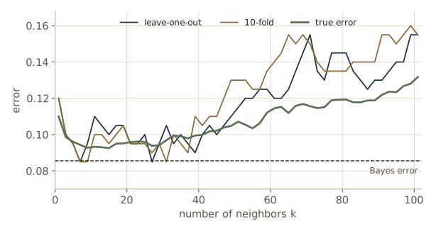
How big should the validation set be? A larger validation set gives a less noisy estimate, but it leaves less data for training, so the estimate describes a classifier trained on fewer points than the one we will use, and is pessimistic. Since the validation set usually sets only one or a few global quantities, while the training set sets all the parameters, the validation fraction \(\gamma\) is usually below one half; \(\gamma = 0.1\) is a common default. The next cell measures the trade-off for the \(k = 15\) rule over 100 training sets of 200 points.
rng_g = np.random.default_rng(43)
rows = {g: [] for g in (0.1, 0.2, 0.3, 0.5)}
for _ in range(100):
    X, y = sample_wave(200, rng_g)
    true_full = expected_error(knn_votes_all_k(sq_dists(X_eval, X), y, [15])[0])
    for g in rows:
        perm = rng_g.permutation(200)
        va, tr = perm[:int(g * 200)], perm[int(g * 200):]
        est = np.mean(knn_votes_all_k(sq_dists(X[va], X[tr]), y[tr], [15])[0] != y[va])
        rows[g].append(est - true_full)
print("gamma   mean(estimate - true)   sd(estimate - true)")
for g, v in rows.items():
    print(f" {g:.1f}         {np.mean(v):+.4f}               {np.std(v):.4f}")
gamma   mean(estimate - true)   sd(estimate - true)
 0.1         -0.0036               0.0699
 0.2         -0.0043               0.0442
 0.3         +0.0041               0.0369
 0.5         +0.0101               0.0312
The spread of the estimate shrinks from 0.070 to 0.031 as \(\gamma\) grows from 0.1 to 0.5, while a pessimistic bias appears (about 0.01 at \(\gamma = 0.5\), when the rule is trained on half the data). Here the variance dominates; with a classifier whose accuracy depends more strongly on the amount of training data, the bias would matter sooner. Cross-validation averages several such splits and so reduces the variance without shrinking the training sets much.
Cross-validation is a heuristic, not a theorem. On some problems it does no good, and one can even construct problems on which anti-cross-validation, choosing the parameter with the highest validation error, works better. That is the no free lunch theorem again.
How precise is a measured error rate? Once the classifier is fixed, each independent test pattern is misclassified with probability \(p\), the true error rate. If \(k\) of \(n'\) test patterns are misclassified, \(k\) is binomial and the maximum-likelihood estimate of \(p\) is \(\hat{p} = k/n'\). Its uncertainty can be large. An exact (Clopper–Pearson) 95% confidence interval collects the values of \(p\) that would make the observed \(k\) unsurprising at the 2.5% level in each tail; its endpoints are quantiles of beta distributions, which scipy.special.betaincinv computes. We check each endpoint against the binomial tail it is defined by.
from scipy.special import betaincinv

def binom_cdf(k, n, p):
    i = np.arange(k + 1)
    logpmf = (gammaln(n + 1) - gammaln(i + 1) - gammaln(n - i + 1)
              + i * np.log(p) + (n - i) * np.log1p(-p))
    return np.exp(logsumexp(logpmf))

def clopper_pearson(k, n, level=0.95):
    a = 1 - level
    lo = 0.0 if k == 0 else betaincinv(k, n - k + 1, a / 2)
    hi = 1.0 if k == n else betaincinv(k + 1, n - k, 1 - a / 2)
    return lo, hi

for k, n in [(0, 50), (0, 300), (5, 50), (50, 500), (500, 5000)]:
    lo, hi = clopper_pearson(k, n)
    print(f"{k:3d} errors in {n:4d}: p_hat = {k / n:.3f}, 95% interval [{lo:.4f}, {hi:.4f}];"
          f"  P(K <= k at upper end) = {binom_cdf(k, n, hi):.4f}")
  0 errors in   50: p_hat = 0.000, 95% interval [0.0000, 0.0711];  P(K <= k at upper end) = 0.0250
  0 errors in  300: p_hat = 0.000, 95% interval [0.0000, 0.0122];  P(K <= k at upper end) = 0.0250
  5 errors in   50: p_hat = 0.100, 95% interval [0.0333, 0.2181];  P(K <= k at upper end) = 0.0250
 50 errors in  500: p_hat = 0.100, 95% interval [0.0751, 0.1297];  P(K <= k at upper end) = 0.0250
500 errors in 5000: p_hat = 0.100, 95% interval [0.0918, 0.1087];  P(K <= k at upper end) = 0.0250
With 50 test patterns and no errors at all, the true error rate could still be as high as 7%; to be confident that it is below about 1%, we need several hundred error-free test patterns. Differences of a percent or two between classifiers are meaningless unless the test set has thousands of patterns.
Jackknife and bootstrap estimates of accuracy
Leave-one-out cross-validation is the jackknife applied to the classification error. It trains \(n\) classifiers, each on all but one point, and tests each on the point it left out. Each of those classifiers is nearly identical to the one trained on all \(n\) points, so the estimate has little bias, though it can be expensive for learning algorithms without a shortcut like the one we used for \(k\)-nearest neighbors. The jackknife also gives a variance. The leave-one-out error is the mean of the per-point losses \(\ell_i \in \{0, 1\}\), and the jackknife variance of a mean is the usual \(s^2/n\).
This lets us compare two classifiers on the same data. Compute the per-point leave-one-out losses of both, take their differences \(d_i = \ell_i^{(1)} - \ell_i^{(2)}\), and compare the mean difference with its standard error. Pairing the losses point by point removes the variation that comes from which points happen to be hard for both. (The \(\ell_i\) are not quite independent, because each classifier shares most of its training data with the others, so the test is approximate.)
def loo_losses_knn(X, y, k):
    D = sq_dists(X, X)
    np.fill_diagonal(D, np.inf)                    # leave each point out of its own neighbors
    return (knn_votes_all_k(D, y, [k])[0] != y).astype(float)

l1, l2 = loo_losses_knn(X_cv, y_cv, 1), loo_losses_knn(X_cv, y_cv, 25)
diff = l1 - l2
se = diff.std(ddof=1) / np.sqrt(len(diff))
print(f"leave-one-out error: k = 1: {l1.mean():.3f} (se {l1.std(ddof=1) / np.sqrt(200):.3f}), "
      f"k = 25: {l2.mean():.3f} (se {l2.std(ddof=1) / np.sqrt(200):.3f})")
print(f"paired difference {diff.mean():.3f}, standard error {se:.3f}, z = {diff.mean() / se:.2f}")
print(f"true errors: k = 1: {true_k[0]:.4f}, k = 25: {true_k[ks == 25][0]:.4f}")
leave-one-out error: k = 1: 0.120 (se 0.023), k = 25: 0.100 (se 0.021)
paired difference 0.020, standard error 0.020, z = 1.00
true errors: k = 1: 0.1100, k = 25: 0.0960
The leave-one-out errors are 0.120 and 0.100, but the paired difference of 0.020 is only one standard error from zero, so these 200 points cannot establish that \(k = 25\) is better, although the true errors (0.110 and 0.096) show that it is. Pairing helps less than usual here because the two rules make rather different mistakes. Differences of a couple of percentage points need far more than 200 test cases to confirm, as the confidence intervals above already suggested.
The bootstrap gives other estimates. Train a classifier on each of \(B\) bootstrap samples and test it on the points not in that sample (on average a fraction \((1 - 1/n)^n \approx e^{-1} \approx 0.368\) of them); averaging over samples gives the out-of-bag error \(\hat{E}_0\). Each bootstrap classifier sees only about 63.2% of the distinct points, so \(\hat{E}_0\) is pessimistic, while the resubstitution error \(\hat{E}_{\text{resub}}\) is optimistic. The .632 estimate mixes them,
\[\hat{E}_{.632} = 0.368\,\hat{E}_{\text{resub}} + 0.632\,\hat{E}_0 .\]For \(k\)-nearest neighbors a bootstrap sample contains repeated points, and a point that appears \(c\) times counts \(c\) times among the neighbors. The cell below handles that with the counts, then compares the estimators over 30 training sets.
def knn_oob_error(X, y, k, B, rng):
    n = len(y)
    order = np.argsort(sq_dists(X, X), axis=1)
    wrong = total = 0
    for _ in range(B):
        c = np.bincount(rng.integers(0, n, n), minlength=n)     # multiplicity of each point
        oob = np.flatnonzero(c == 0)
        cnt = c[order[oob]]                                   # counts along each neighbor list
        before = np.cumsum(cnt, axis=1) - cnt
        take = np.clip(k - before, 0, cnt)                    # copies used among the k nearest
        pred = (np.sum(take * y[order[oob]], axis=1) > k / 2).astype(int)
        wrong += np.sum(pred != y[oob])
        total += len(oob)
    return wrong / total

rng_e = np.random.default_rng(44)
est = {"resubstitution": [], "leave-one-out": [], "10-fold": [], "bootstrap E0": [], ".632": []}
truth = []
for _ in range(30):
    X, y = sample_wave(200, rng_e)
    truth.append(expected_error(knn_votes_all_k(sq_dists(X_eval, X), y, [15])[0]))
    resub = np.mean(knn_votes_all_k(sq_dists(X, X), y, [15])[0] != y)
    e0 = knn_oob_error(X, y, 15, 50, rng_e)
    est["resubstitution"].append(resub)
    est["leave-one-out"].append(loo_losses_knn(X, y, 15).mean())
    folds = np.array_split(rng_e.permutation(200), 10)
    est["10-fold"].append(knn_cv_errors(X, y, [15], folds)[0])
    est["bootstrap E0"].append(e0)
    est[".632"].append(0.368 * resub + 0.632 * e0)
truth = np.array(truth)
print(f"average true error {truth.mean():.4f}")
print("estimator         mean - true   rms error")
for name, v in est.items():
    v = np.array(v)
    print(f"{name:16s}   {np.mean(v - truth):+.4f}      {np.sqrt(np.mean((v - truth)**2)):.4f}")
average true error 0.0997
estimator         mean - true   rms error
resubstitution     -0.0130      0.0266
leave-one-out      +0.0010      0.0246
10-fold            +0.0011      0.0254
bootstrap E0       +0.0099      0.0271
.632               +0.0015      0.0239
Resubstitution is optimistic, by about 0.013 on average. Leave-one-out and 10-fold cross-validation are nearly unbiased, and the out-of-bag error is pessimistic by about 0.01 because its classifiers see fewer distinct points. The .632 correction removes most of that pessimism; its original motivation was precisely this. Every estimator has an rms error of about 0.025, mostly variance, which is the price of 200 points; the .632 estimate is marginally the most accurate here. The ranking of these estimators changes from problem to problem and classifier to classifier; for a nearest-neighbor rule with \(k = 1\), for instance, the resubstitution error is zero and the .632 estimate is pulled down by it.
Maximum-likelihood model comparison
Cross-validation compares classifiers by their predictions. When the candidate models are probabilistic, we can also compare them by how well they explain the training data. Let \(h_1, h_2, \dots\) be candidate models (hypotheses), each with its own parameter vector \(\boldsymbol{\theta}\). Bayes’ rule over models gives
\[P(h_i \mid \mathcal{D}) = \frac{p(\mathcal{D} \mid h_i)\,P(h_i)}{p(\mathcal{D})} \propto p(\mathcal{D} \mid h_i)\,P(h_i).\]The data-dependent factor \(p(\mathcal{D} \mid h_i)\) is the evidence for \(h_i\). The prior over models is usually taken as uniform and dropped, so models are compared by their evidence. Maximum-likelihood model comparison (also called ML-II) replaces the evidence by the likelihood at the maximum-likelihood parameters, \(p(\mathcal{D} \mid \hat{\boldsymbol{\theta}}, h_i)\), and picks the model with the largest value.
For nested models that fails outright: a model that contains another can always fit at least as well, so maximized likelihood always picks the most flexible candidate. The evidence corrects this, as we see next.
Bayesian model comparison and the Occam factor
The evidence integrates the likelihood over the prior instead of maximizing it:
\[p(\mathcal{D} \mid h_i) = \int p(\mathcal{D} \mid \boldsymbol{\theta}, h_i)\,p(\boldsymbol{\theta} \mid h_i)\,d\boldsymbol{\theta}.\]When the likelihood is sharply peaked at \(\hat{\boldsymbol{\theta}}\), with a width \(\Delta\theta\) in parameter space, and the prior is spread over a much wider range \(\Delta^0\theta\) with density about \(1/\Delta^0\theta\), the integral is about the peak height times its width:
\[p(\mathcal{D} \mid h_i) \approx \underbrace{p(\mathcal{D} \mid \hat{\boldsymbol{\theta}}, h_i)}_{\text{best-fit likelihood}}\ \underbrace{p(\hat{\boldsymbol{\theta}} \mid h_i)\,\Delta\theta}_{\text{Occam factor}}, \qquad \text{Occam factor} \approx \frac{\Delta\theta}{\Delta^0\theta}.\]The Occam factor is the fraction of the prior’s parameter volume that remains compatible with the data. It is less than one, and it is smaller for a model with more parameters or a vaguer prior, whose prior volume collapses more when the data arrive. So a more complex model must earn its extra flexibility with a better fit, and “too complex” is judged relative to the data. With \(p\) parameters and a Gaussian approximation to the peak (the Laplace approximation),
\[p(\mathcal{D} \mid h_i) \approx p(\mathcal{D} \mid \hat{\boldsymbol{\theta}}, h_i)\ p(\hat{\boldsymbol{\theta}} \mid h_i)\,(2\pi)^{p/2}\,\lvert \mathbf{H} \rvert^{-1/2}, \qquad \mathbf{H} = -\nabla\nabla \ln p(\boldsymbol{\theta} \mid \mathcal{D}, h_i)\big\rvert_{\hat{\boldsymbol{\theta}}},\]where the Hessian \(\mathbf{H}\) measures how sharply the posterior is peaked. Keeping only the terms that grow with \(n\) gives the Bayesian information criterion, \(\ln p(\mathcal{D} \mid h_i) \approx \ln p(\mathcal{D} \mid \hat{\boldsymbol{\theta}}, h_i) - \frac{p}{2}\ln n\). If the model is degenerate, with several parameter settings giving the same classifier (as with the hidden units of a network, which can be permuted), the Occam factor should be multiplied by the number of equivalent settings.
For linear regression with a Gaussian prior on the weights, the posterior is exactly Gaussian and the Laplace formula is exact. We compare polynomial degrees on one training set of 30 points from the regression problem of the bias–variance section, with the noise level known and a unit Gaussian prior on the Legendre coefficients. The table shows the maximized log likelihood (ML-II), the best-fit log likelihood at the posterior mode and the log Occam factor (which add up to the log evidence), and the BIC. Intro to ML, module 03 derives the evidence of this model in detail and also shows how to estimate the prior and noise precisions from the data.
rng_ev = np.random.default_rng(45)
n_ev = 30
x_ev = rng_ev.uniform(-1, 1, n_ev)
t_ev = F_reg(x_ev) + sigma_reg * rng_ev.standard_normal(n_ev)
alpha_ev, beta_ev = 1.0, 1 / sigma_reg**2          # prior precision, noise precision

print("degree  ln L(ML)   ln L(mode)  ln Occam   ln evidence     BIC")
scores = []
for M in range(10):
    Phi = np.polynomial.legendre.legvander(x_ev, M)
    p = M + 1
    w_ml = fit_poly(x_ev, t_ev, M)
    def lnL(w):
        rss = np.sum((t_ev - Phi @ w)**2)
        return 0.5 * n_ev * np.log(beta_ev / (2 * np.pi)) - 0.5 * beta_ev * rss
    A = alpha_ev * np.eye(p) + beta_ev * Phi.T @ Phi       # posterior precision = Hessian H
    m = beta_ev * np.linalg.solve(A, Phi.T @ t_ev)         # posterior mode
    ln_prior_m = 0.5 * p * np.log(alpha_ev / (2 * np.pi)) - 0.5 * alpha_ev * m @ m
    ln_occam = ln_prior_m + 0.5 * p * np.log(2 * np.pi) - 0.5 * np.linalg.slogdet(A)[1]
    ln_ev = lnL(m) + ln_occam
    # the same evidence from the marginal distribution t ~ N(0, Phi Phi^t / alpha + I / beta)
    C = Phi @ Phi.T / alpha_ev + np.eye(n_ev) / beta_ev
    ln_ev_direct = -0.5 * (n_ev * np.log(2 * np.pi) + np.linalg.slogdet(C)[1]
                           + t_ev @ np.linalg.solve(C, t_ev))
    assert np.isclose(ln_ev, ln_ev_direct)
    bic = lnL(w_ml) - 0.5 * p * np.log(n_ev)
    scores.append((M, lnL(w_ml), ln_ev, bic))
    print(f"{M:4d}   {lnL(w_ml):8.2f}   {lnL(m):8.2f}   {ln_occam:8.2f}   {ln_ev:9.2f}   {bic:8.2f}")
print("chosen degree: ML-II", max(scores, key=lambda s: s[1])[0],
      "  evidence", max(scores, key=lambda s: s[2])[0], "  BIC", max(scores, key=lambda s: s[3])[0])
degree  ln L(ML)   ln L(mode)  ln Occam   ln evidence     BIC
   0     -95.36     -95.36      -2.93      -98.30     -97.06
   1     -10.88     -10.89      -6.05      -16.94     -14.28
   2     -10.59     -10.60      -8.08      -18.68     -15.69
   3      -1.73      -1.75      -9.96      -11.71      -8.54
   4      -0.04      -0.07     -11.78      -11.85      -8.54
   5       0.34       0.30     -13.31      -13.00      -9.87
   6       0.48       0.42     -14.40      -13.98     -11.43
   7       0.89       0.83     -15.16      -14.33     -12.72
   8       1.50       1.32     -16.10      -14.78     -13.81
   9       1.51       1.28     -16.64      -15.36     -15.50
chosen degree: ML-II 9   evidence 3   BIC 3
The maximized likelihood rises with every degree, so ML-II picks the most complex model on the list. The log Occam factor falls steadily, by between half a nat and three nats per added parameter, and the evidence, which balances the two, peaks at degree 3, just ahead of degree 4. BIC ties degrees 3 and 4 to two decimals and also picks 3. This matches the bias–variance experiment, where degree 3 had the lowest expected test error. The assertion checks the Laplace formula against the evidence computed directly from the marginal Gaussian distribution of the targets: for this model they agree exactly. Note what the evidence does not use: any held-out data. It judges the model by how well it predicted the training data before seeing them, which is a different question from cross-validation’s, and the two can disagree.
Bayesian model selection and no free lunch
Bayesian model selection looks like exactly the principled way of choosing algorithms that the no free lunch theorem rules out. Imagine a composite algorithm that uses the evidence to choose between two learning algorithms and applies the winner, and a perverse twin that applies the loser. The first seems bound to beat the second on every problem.
The resolution is the prior. Comparing models by their evidence assumes a uniform prior over the candidate models, and a uniform prior over models is not a uniform prior over target functions: the targets that the chosen models represent easily get much more prior mass than the rest. So Bayesian model selection corresponds to a particular nonuniform prior over targets, which depends on how the candidate models were chosen and parameterized, and the no free lunch theorem allows an algorithm to beat chance under a nonuniform prior. Statisticians are cautious about the principle of indifference (assuming a uniform prior because we know nothing) for exactly this reason: uniform in one parameterization is far from uniform in another. The empirical success of Bayesian model selection says that the priors it implies match many real problems.
The problem-average error rate
How does the error rate depend on the number of samples \(n\) and on the complexity of the classifier, averaged over problems? One classical analysis makes the problem discrete. Divide feature space into \(m\) cells, and describe a two-category problem with equal priors by the cell probabilities \(p_i = P(\mathbf{x} \in \text{cell } i \mid \omega_1)\) and \(q_i = P(\mathbf{x} \in \text{cell } i \mid \omega_2)\). The Bayes error is \(\frac{1}{2}\sum_i \min(p_i, q_i)\). A classifier trained on \(n/2\) samples per class labels each cell by its majority class; its error depends on the problem and on the counts.
To remove the dependence on the problem, average over problems: draw \(\mathbf{p}\) and \(\mathbf{q}\) uniformly from the probability simplex, as a stand-in for “all problems”, and average the expected error. (This uniform distribution over \(\mathbf{p}\) and \(\mathbf{q}\) is itself a choice of prior, and not the uniform prior over targets of the no free lunch theorem.) The cell below does this by simulation, breaking ties in a cell by a coin flip.
def problem_average_error(m, n_per, n_problems, rng):
    P = rng.dirichlet(np.ones(m), n_problems)           # p for each problem
    Q = rng.dirichlet(np.ones(m), n_problems)
    if n_per is None:                                   # infinite data: the Bayes error
        return np.mean(0.5 * np.sum(np.minimum(P, Q), axis=1))
    N1, N2 = rng.multinomial(n_per, P), rng.multinomial(n_per, Q)
    err = np.where(N1 > N2, Q, np.where(N1 < N2, P, 0.5 * (P + Q)))
    return np.mean(0.5 * np.sum(err, axis=1))

rng_pa = np.random.default_rng(46)
cells = [1, 2, 4, 8, 16, 32, 64, 128, 512, 2048]
print("  m    " + "  ".join(f"{c:6d}" for c in cells))
for n_per in (10, 50, 250, None):
    row = [problem_average_error(m, n_per, 1000, rng_pa) for m in cells]
    label = "inf" if n_per is None else str(2 * n_per)
    print(f"n={label:4s} " + "  ".join(f"{r:6.3f}" for r in row))
  m         1       2       4       8      16      32      64     128     512    2048
n=20    0.500   0.345   0.329   0.330   0.361   0.404   0.442   0.465   0.491   0.498
n=100   0.500   0.334   0.292   0.282   0.289   0.315   0.348   0.390   0.459   0.488
n=500   0.500   0.337   0.287   0.266   0.267   0.270   0.280   0.302   0.376   0.451
n=inf   0.500   0.331   0.283   0.264   0.259   0.255   0.251   0.251   0.250   0.250
With unlimited data the average error falls from one half (one cell: only the priors are available) toward one quarter as \(m\) grows; the average is high because the uniform prior includes many hopeless problems. With a finite sample every row has an optimal number of cells: about 4 for 20 samples, 8 for 100, and a broad optimum from 8 to 32 for 500. At first more cells separate the classes better, but eventually most cells are empty or nearly so, the classifier falls back on guessing, and the error returns toward one half. The specific numbers depend entirely on the prior over problems and mean little for any particular problem. The lesson is qualitative: for a fixed amount of data, making the classifier finer (more cells, more features, more parameters) eventually raises the variance enough to make things worse. If the cells come from cutting each of \(d\) features into two, \(m = 2^d\), and the best \(m\) for a few hundred samples corresponds to only a handful of binary features.
Predicting final performance from learning curves
Training on a very large data set can take a long time, and comparing several classifiers that way can take much longer. It would help to predict from small training sets how each classifier will do on the full set, and then fully train only the most promising one. A learning curve, here the test error of a classifier fully trained on \(n'\) points plotted against \(n'\), often decays like a power law,
\[E_{\text{test}}(n') \approx a + \frac{b}{n'^{\alpha}},\]with \(a\), \(b\), and \(\alpha\) depending on the problem and the classifier. As \(n' \to \infty\) training and test error approach the same limit \(a\), which is the Bayes error if the classifier is flexible enough. The training error rises toward \(a\) from below, and can be modeled the same way, \(E_{\text{train}}(n') \approx a - c/n'^{\beta}\). If \(\alpha = \beta\) and \(b = c\), the two curves are mirror images:
\[\frac{E_{\text{test}} + E_{\text{train}}}{2} \approx a, \qquad E_{\text{test}} - E_{\text{train}} \approx \frac{2b}{n'^{\alpha}},\]so the average of training and test error estimates \(a\) directly, and the difference is a straight line on a log–log plot. Even when these assumptions are only rough, both curves can be fitted and the asymptotes compared.
We try this on the quadratic Gaussian classifier for the two-class problem of the bias–variance section, whose Bayes error we know. We measure the average training and test errors for training sets of 5 to 40 points per class, fit \(a + b\,n'^{-\alpha}\) to the test errors (a grid over \(\alpha\), with \(a\) and \(b\) by linear least squares for each \(\alpha\)), and extrapolate to much larger training sets.
X_lc, _ = sample_classes(5000, np.random.default_rng(47))
F_lc = true_posterior(X_lc)
bayes_lc = np.mean(np.minimum(F_lc, 1 - F_lc))

def learning_point(n_per, reps, rng):
    tr, te = [], []
    for _ in range(reps):
        X, y = sample_classes(n_per, rng)
        model = fit_gauss(X, y, "quadratic")
        tr.append(np.mean((gauss_posterior(model, X) > 0.5) != y))
        pred = gauss_posterior(model, X_lc) > 0.5
        te.append(np.mean(np.where(pred, 1 - F_lc, F_lc)))
    return np.mean(tr), np.mean(te)

def fit_power_law(n, E):
    """Fit E = a + b n^(-alpha): grid over alpha, linear least squares for (a, b)."""
    best = None
    for alpha in np.linspace(0.1, 3.0, 291):
        Z = np.column_stack([np.ones(len(n)), n**(-alpha)])
        coef, *_ = np.linalg.lstsq(Z, E, rcond=None)
        sse = np.sum((Z @ coef - E)**2)
        if best is None or sse < best[0]:
            best = (sse, coef[0], coef[1], alpha)
    return best[1:]

rng_lc = np.random.default_rng(48)
small = np.array([5, 7, 10, 14, 20, 28, 40])
curve = np.array([learning_point(m, 60, rng_lc) for m in small])
a_fit, b_fit, alpha_fit = fit_power_law(2.0 * small, curve[:, 1])
print(f"fit on 10-80 points: a = {a_fit:.4f}, b = {b_fit:.3f}, alpha = {alpha_fit:.2f};  "
      f"Bayes error {bayes_lc:.4f}")
print(f"(train + test)/2 at the largest small size: {curve[-1].mean():.4f}")
print("  n'   predicted test error   measured test error   measured train error")
for m in (100, 300, 1000):
    tr, te = learning_point(m, 10, rng_lc)
    print(f"{2 * m:5d}        {a_fit + b_fit * (2 * m)**(-alpha_fit):.4f}               "
          f"{te:.4f}                {tr:.4f}")
fit on 10-80 points: a = 0.1952, b = 0.980, alpha = 0.95;  Bayes error 0.2028
(train + test)/2 at the largest small size: 0.2077
  n'   predicted test error   measured test error   measured train error
  200        0.2015               0.2058                0.1905
  600        0.1974               0.2038                0.1942
 2000        0.1959               0.2031                0.2030
The fitted asymptote from training sets of at most 80 points, 0.195, is a little below the Bayes error of 0.203, so the extrapolation is slightly optimistic: it predicts 0.196 at 2000 points where we measure 0.203. The cruder estimate, the average of training and test errors at 80 points, is 0.208, about as close from the other side. Both are within one percentage point of the truth, from data 25 times smaller than the largest training set, which is enough to rank classifiers whose asymptotes differ by more than that. To compare classifiers this way, fit a curve for each on small training sets and train only the one with the lowest predicted asymptote (or the lowest predicted error at the size we can afford). The method can mislead when the curves cross late, which is common: a flexible classifier often loses on small sets and wins on large ones, exactly as in the bias–variance experiment earlier.
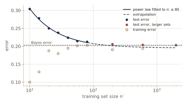
The capacity of a separating plane
How many points can a linear classifier fit before fitting them says something? Take \(n\) points in \(d\) dimensions in general position (no \(d + 1\) of them lie on a common hyperplane), and consider all \(2^n\) ways of labeling them. A labeling is a linear dichotomy if some hyperplane \(\mathbf{w}^{t}\mathbf{x} + w_0 = 0\) separates the two labels. Cover’s function-counting theorem says the number of linear dichotomies does not depend on where the points are, as long as they are in general position, and that the fraction of dichotomies that are linear is
\[f(n, d) = \begin{cases} 1, & n \le d + 1, \\[4pt] \dfrac{2}{2^n}\displaystyle\sum_{i=0}^{d}\binom{n-1}{i}, & n > d + 1. \end{cases}\](The second formula also gives 1 when \(n \le d + 1\).) A short recursion proves it: adding an \(n\)th point to \(n - 1\) points, each linear dichotomy of the old points extends in either one or two ways, and it extends in two ways exactly when some separating hyperplane can be made to pass through the new point, which is counting linear dichotomies in one dimension less. The count \(C(n, d)\) therefore satisfies \(C(n, d) = C(n - 1, d) + C(n - 1, d - 1)\), whose solution is \(2\sum_{i=0}^{d}\binom{n-1}{i}\).
We can check the formula without linear programming. For points in general position and \(n > d\), every separable labeling can be realized by a hyperplane that passes through exactly \(d\) of the points, with those \(d\) points assigned to either side by an arbitrarily small tilt. (The separating hyperplanes form an open cone in the \((d + 1)\)-dimensional space of \((\mathbf{w}, w_0)\), and an edge of that cone touches exactly \(d\) of the points.) So we enumerate the hyperplanes through each \(d\)-subset, record the sides of the other points, and give the \(d\) points on the plane every possible assignment.
def cover_fraction(n, d):
    return 1.0 if n <= d + 1 else 2 * sum(comb(n - 1, i) for i in range(d + 1)) / 2**n

def count_linear_dichotomies(X):
    n, d = X.shape
    found = set()
    for S in itertools.combinations(range(n), d):
        # hyperplane through the d points of S: solve [x 1] (w, w0) = 0 via the null space
        A = np.column_stack([X[list(S)], np.ones(d)])
        v = np.linalg.svd(A)[2][-1]                       # (w, w0) spanning the null space
        side = np.sign(X @ v[:-1] + v[-1])
        for assign in itertools.product([-1, 1], repeat=d):
            lab = side.copy()
            lab[list(S)] = assign
            found.add(tuple(lab))
            found.add(tuple(-lab))
    return len(found)

rng_cov = np.random.default_rng(49)
print(" d   n   enumerated   formula 2^n f(n,d)")
for d_c, n_list in [(1, [3, 4, 6]), (2, [4, 6, 8, 10]), (3, [6, 8, 10])]:
    for n_c in n_list:
        X = rng_cov.standard_normal((n_c, d_c))
        formula = round(cover_fraction(n_c, d_c) * 2**n_c)
        print(f"{d_c:2d} {n_c:3d} {count_linear_dichotomies(X):10d} {formula:12d}")
print("f(2(d+1), d) for d = 1, 5, 50:", [cover_fraction(2 * (d + 1), d) for d in (1, 5, 50)])
 d   n   enumerated   formula 2^n f(n,d)
 1   3          6            6
 1   4          8            8
 1   6         12           12
 2   4         14           14
 2   6         32           32
 2   8         58           58
 2  10         92           92
 3   6         52           52
 3   8        128          128
 3  10        260          260
f(2(d+1), d) for d = 1, 5, 50: [0.5, 0.5, 0.5]
The enumeration matches the formula in every case, and \(f(2(d + 1), d) = 1/2\) exactly for every \(d\), since the sum then covers exactly half of the binomial coefficients \(\binom{2d+1}{i}\). For example, with \(d = 1\) and four points on a line, 8 of the 16 labelings can be separated by a single threshold: those with one change of label along the line or none.
The number \(2(d + 1)\) is called the capacity of a hyperplane in \(d\) dimensions. Below it, most labelings of a random set of points are linearly separable, so a linear classifier that fits the training data perfectly has learned almost nothing: it would have fit random labels too. The transition sharpens as \(d\) grows: for large \(d\), almost every labeling of fewer than \(2(d + 1)\) points is separable and almost none of more. A hyperplane is not really constrained by the data until \(n\) is several times \(d + 1\), which is sometimes summarized as “generalization begins only after learning ends”, meaning after the classifier can no longer fit arbitrary labels. Turned around: in this average sense, a linear classifier should not be expected to fit a problem’s structure when \(d\) exceeds about \(n/2 - 1\).
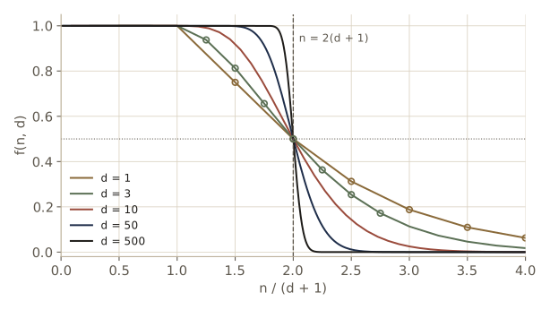
Combining classifiers
Bagging and boosting combine components of one kind trained on different versions of the data. More generally, a classifier whose decision is built from the outputs of several component classifiers goes by many names: ensemble classifier, modular classifier, pooled classifier, or mixture of experts. Combining pays off most when the components are good in different ways, for instance when each is an expert on its own region of feature space, or when they use different features or different kinds of models, so that their errors are not the same.
Component classifiers with discriminant functions
Suppose the data come from a mixture of processes. For each input \(\mathbf{x}\), one of \(k\) processes \(r\) is chosen with probability \(P(r \mid \mathbf{x}, \boldsymbol{\theta}_0)\), and that process emits the label \(y\) with probability \(P(y \mid \mathbf{x}, \boldsymbol{\theta}_r)\). Overall,
\[P(y \mid \mathbf{x}, \boldsymbol{\Theta}) = \sum_{r=1}^{k} P(r \mid \mathbf{x}, \boldsymbol{\theta}_0)\,P(y \mid \mathbf{x}, \boldsymbol{\theta}_r), \qquad \boldsymbol{\Theta} = (\boldsymbol{\theta}_0, \boldsymbol{\theta}_1, \dots, \boldsymbol{\theta}_k).\]The mixture-of-experts architecture mirrors this: \(k\) component classifiers (the experts), each producing discriminant values \(g_{ri} = \hat{P}(\omega_i \mid \mathbf{x}, \boldsymbol{\theta}_r)\) that sum to one over the categories, and a gating subsystem that produces weights \(w_r = P(r \mid \mathbf{x}, \boldsymbol{\theta}_0)\), summing to one over the experts, which say how much to trust each expert at this \(\mathbf{x}\). The pooled output is \(\sum_r w_r g_{ri}\), and we choose the category with the largest pooled value.
Training maximizes the log likelihood of the \(n\) training patterns,
\[l(\mathcal{D}, \boldsymbol{\Theta}) = \sum_{i=1}^{n} \ln\left[\sum_{r=1}^{k} P(r \mid \mathbf{x}^i, \boldsymbol{\theta}_0)\,P(y_i \mid \mathbf{x}^i, \boldsymbol{\theta}_r)\right].\]Differentiating the logarithm of a sum gives the posterior probability that process \(r\) produced pattern \(i\),
\[P(r \mid y_i, \mathbf{x}^i) = \frac{P(r \mid \mathbf{x}^i, \boldsymbol{\theta}_0)\,P(y_i \mid \mathbf{x}^i, \boldsymbol{\theta}_r)}{\sum_{s} P(s \mid \mathbf{x}^i, \boldsymbol{\theta}_0)\,P(y_i \mid \mathbf{x}^i, \boldsymbol{\theta}_s)},\]and the gradients
\[\frac{\partial l}{\partial \boldsymbol{\theta}_r} = \sum_{i=1}^{n} P(r \mid y_i, \mathbf{x}^i)\,\frac{\partial}{\partial \boldsymbol{\theta}_r}\ln P(y_i \mid \mathbf{x}^i, \boldsymbol{\theta}_r), \qquad \frac{\partial l}{\partial u_r^i} = P(r \mid y_i, \mathbf{x}^i) - w_r^i,\]where \(u_r^i\) is the gating network’s input to a softmax, \(w_r^i = e^{u_r^i}/\sum_s e^{u_s^i}\). Each expert is trained on every pattern, weighted by the posterior probability that it is responsible for that pattern; and the gating weights are pushed from their prior values \(w_r\) toward the posterior responsibilities. The same responsibilities are the E step of an EM algorithm for this model, whose M step fits each expert to its weighted patterns (module 03 has EM in general, and Intro to ML, module 14 trains mixtures of experts that way).
We fit two logistic-regression experts with a linear softmax gate by plain gradient ascent, on a noisy version of the exclusive-or problem: \(\omega_1\) where \(x_1 x_2 > 0\), with 5% label noise. No single linear classifier can do better than chance on it, but the gate can split the plane along one axis and let each expert draw a line through its own half. We check the analytic gradient by finite differences first.
def F_xor(X):
    return np.where(X[:, 0] * X[:, 1] > 0, 0.95, 0.05)

def moe_parts(A, V, Y):
    """A: expert weights (k, 3); V: gating weights (k, 3); Y: augmented inputs (n, 3)."""
    act = Y @ A.T
    log_p1, log_p0 = -np.logaddexp(0, -act), -np.logaddexp(0, act)   # ln P(y = 1), ln P(y = 0)
    log_w = Y @ V.T
    log_w -= logsumexp(log_w, axis=1, keepdims=True)                 # ln gating weights
    return act, log_p1, log_p0, log_w

def moe_loglik(A, V, Y, y):
    _, lp1, lp0, lw = moe_parts(A, V, Y)
    return np.sum(logsumexp(lw + np.where(y[:, None] == 1, lp1, lp0), axis=1))

def moe_grad(A, V, Y, y):
    act, lp1, lp0, lw = moe_parts(A, V, Y)
    lh = lw + np.where(y[:, None] == 1, lp1, lp0)
    Hr = np.exp(lh - logsumexp(lh, axis=1, keepdims=True))          # P(r | y_i, x_i)
    gA = (Hr * (y[:, None] - expit(act))).T @ Y                      # experts
    gV = (Hr - np.exp(lw)).T @ Y                                     # gate
    return gA, gV

def moe_prob(A, V, X):
    _, lp1, _, lw = moe_parts(A, V, np.column_stack([np.ones(len(X)), X]))
    return np.exp(logsumexp(lw + lp1, axis=1))

rng_moe = np.random.default_rng(60)
X_x = rng_moe.uniform(-2, 2, (400, 2))
y_x = (rng_moe.uniform(0, 1, 400) < F_xor(X_x)).astype(int)
Y_x = np.column_stack([np.ones(400), X_x])
F_x_eval = F_xor(X_eval)

A_m, V_m = 0.1 * rng_moe.standard_normal((2, 3)), 0.1 * rng_moe.standard_normal((2, 3))
gA, gV = moe_grad(A_m, V_m, Y_x, y_x)
eps, fd = 1e-6, []
for M, G, idx in [(A_m, gA, (0, 1)), (V_m, gV, (1, 2))]:
    M[idx] += eps
    up = moe_loglik(A_m, V_m, Y_x, y_x)
    M[idx] -= 2 * eps
    down = moe_loglik(A_m, V_m, Y_x, y_x)
    M[idx] += eps
    fd.append(((up - down) / (2 * eps), G[idx]))
print("finite difference vs analytic:", [f"{a:.6f} / {b:.6f}" for a, b in fd])

for it in range(1501):
    gA, gV = moe_grad(A_m, V_m, Y_x, y_x)
    A_m += 0.5 * gA / 400
    V_m += 0.5 * gV / 400
    if it in (0, 100, 500, 1500):
        p = moe_prob(A_m, V_m, X_eval)
        print(f"iteration {it:4d}: mean log likelihood {moe_loglik(A_m, V_m, Y_x, y_x) / 400:.4f}, "
              f"expected error {np.mean(np.where(p > 0.5, 1 - F_x_eval, F_x_eval)):.4f}")
a_single = fit_logistic(X_x, y_x)
p_single = expit(a_single[0] + X_eval @ a_single[1:])
err_single = np.mean(np.where(p_single > 0.5, 1 - F_x_eval, F_x_eval))
print(f"single logistic regression: {err_single:.4f};"
      f"  Bayes error 0.0500")
print("gate weights (w0, w1, w2) for expert 1 minus expert 2:", V_m[0] - V_m[1])
finite difference vs analytic: ['-5.683992 / -5.683992', '6.471572 / 6.471572']
iteration    0: mean log likelihood -0.6982, expected error 0.4570
iteration  100: mean log likelihood -0.3558, expected error 0.0739
iteration  500: mean log likelihood -0.3084, expected error 0.0822
iteration 1500: mean log likelihood -0.2917, expected error 0.0829
single logistic regression: 0.4849;  Bayes error 0.0500
gate weights (w0, w1, w2) for expert 1 minus expert 2: [ -0.3463  -0.1104 -10.867 ]
The analytic gradient matches the finite differences. A single linear classifier is no better than a coin on this problem (error 0.485), while the mixture of two linear experts brings the error down to about 0.08, against a Bayes error of 0.05. The gating weights show how: the difference between the two gate rows depends almost entirely on \(x_2\), with a large coefficient, so the gate hands the upper half of the plane to one expert and the lower half to the other, and each expert draws its line along \(x_1 = 0\). (The problem is symmetric, so a split on \(x_1\) would have worked equally well; the random start decided.) The likelihood keeps rising after about 100 iterations while the error creeps up slightly, a mild case of overfitting 400 points.
Instead of pooling, a winner-take-all rule uses the decision of the single most confident component, the one with the largest \(g_{ri}\). It is suboptimal in general but simple, and it works well when the experts cover separate regions.
How many experts? If we knew the number of processes in the mixture we would use it. Otherwise the number is one more knob on bias and variance to be set by trial or cross-validation; in practice a few too many experts usually do less harm than too few, because the extra ones tend to duplicate each other.
Component classifiers without discriminant functions
Sometimes the components are already trained and of different kinds: a \(k\)-nearest-neighbor rule, a tree, a neural network, a rule-based system. Some give an analog value for each category, some only a ranking of the categories, and some only a single label. To pool them, we first convert every output into \(c\) nonnegative values that sum to one:
- analog outputs \(g_i\): apply the softmax, \(\tilde{g}_i = e^{g_i} / \sum_{j=1}^{c} e^{g_j}\);
- rank order: give the top-ranked category \(c\) points, the next \(c - 1\), and so on down to 1 for the last, and divide by \(c(c+1)/2\) so the values sum to one;
- one-of-\(c\) (a single label): set \(\tilde{g}_i = 1\) for the chosen category and 0 for the others.
Then any of the pooling rules can be applied. Common choices, all simple enough to need no training:
- majority vote: each component votes for its top category;
- Borda count: each component gives \(c - 1\) points to its top category, \(c - 2\) to the next, down to 0; the category with the most points wins;
- sum rule: add the converted values \(\tilde{g}_{ri}\) over components (the mixture of experts with equal, fixed gate weights);
- product rule: multiply them, which is the Bayes-optimal combination of posteriors when the components’ inputs are conditionally independent given the class. Any component that gives a category a value near zero vetoes it, so the product rule suits probabilistic outputs and not one-of-\(c\) outputs.
If the gate weights are to depend on \(\mathbf{x}\), the components can be held fixed and only the gating network trained, with the gradient above.
We build three components for a three-category problem in four dimensions. The classes are Gaussian with unit variances and independent features, and the three components look at different features: a nearest-mean classifier on \((x_1, x_2)\) that reports analog scores (minus half the squared distance to each mean), a quadratic Gaussian classifier on \((x_3, x_4)\) that reports only a ranking of the categories, and a 1-nearest-neighbor rule on \((x_1, x_4)\) that reports only a label. Each is trained on 30 patterns per class. First the conversions for one test pattern, then the accuracy of each component and each pooling rule on 6000 test patterns. For the Borda count, the label-only component gives its \(c - 1\) points to its label and none to the other categories.
M3 = np.array([[0.0, 0.0, 0.0, 0.0], [1.5, 0.5, 1.2, 0.3], [0.5, 1.5, 0.2, 1.4]])

def sample3(n_per, rng):
    X = np.vstack([M3[c] + rng.standard_normal((n_per, 4)) for c in range(3)])
    return X, np.repeat(np.arange(3), n_per)

rng_c3 = np.random.default_rng(62)
X3tr, y3tr = sample3(30, rng_c3)
X3te, y3te = sample3(2000, rng_c3)
c3 = 3

f12, f34, f14 = [0, 1], [2, 3], [0, 3]
means12 = np.array([X3tr[y3tr == c][:, f12].mean(axis=0) for c in range(c3)])
analog = -0.5 * sq_dists(X3te[:, f12], means12)                     # component 1: analog scores
quad = np.column_stack([gauss_logpdf(X3te[:, f34], X3tr[y3tr == c][:, f34].mean(axis=0),
                                     np.cov(X3tr[y3tr == c][:, f34].T, bias=True))
                        for c in range(c3)])
ranks = np.argsort(np.argsort(-quad, axis=1), axis=1)                # component 2: rank 0 = best
label = y3tr[np.argmin(sq_dists(X3te[:, f14], X3tr[:, f14]), axis=1)]  # component 3: a label

g_analog = np.exp(analog - logsumexp(analog, axis=1, keepdims=True))  # softmax
g_rank = (c3 - ranks) / (c3 * (c3 + 1) / 2)
g_label = np.eye(c3)[label]
i0 = 7
print("true class", y3te[i0])
print("  analog scores", analog[i0], "-> softmax", g_analog[i0])
print("  ranks (0 = best)", ranks[i0], "-> rank values", g_rank[i0])
print("  label", label[i0], "-> one-of-c", g_label[i0])

tops = np.column_stack([analog.argmax(axis=1), ranks.argmin(axis=1), label])
votes = np.eye(c3)[tops].sum(axis=1)
sum_rule = g_analog + g_rank + g_label
majority = np.where(votes.max(axis=1) > 1, votes.argmax(axis=1), sum_rule.argmax(axis=1))
rank_analog = np.argsort(np.argsort(-analog, axis=1), axis=1)
borda = (c3 - 1 - rank_analog) + (c3 - 1 - ranks) + (c3 - 1) * g_label
post_quad = np.exp(quad - logsumexp(quad, axis=1, keepdims=True))   # if component 2 gave posteriors
acc = lambda pred: np.mean(pred == y3te)

print(f"\ncomponents: nearest mean (x1, x2) {acc(tops[:, 0]):.3f}, quadratic (x3, x4) "
      f"{acc(tops[:, 1]):.3f}, 1-NN (x1, x4) {acc(tops[:, 2]):.3f}")
print(f"all three: majority vote {acc(majority):.3f}, Borda count {acc(borda.argmax(axis=1)):.3f}, "
      f"sum rule {acc(sum_rule.argmax(axis=1)):.3f}")
print(f"components 1 and 2 as posteriors: sum rule {acc((g_analog + post_quad).argmax(axis=1)):.3f}, "
      f"product rule {acc((np.log(g_analog) + np.log(post_quad)).argmax(axis=1)):.3f}")
print(f"Bayes rule on all four features: {acc(np.argmin(sq_dists(X3te, M3), axis=1)):.3f}")
true class 0
  analog scores [-0.3926 -2.3959 -1.085 ] -> softmax [0.6115 0.0825 0.306 ]
  ranks (0 = best) [1 2 0] -> rank values [0.3333 0.1667 0.5   ]
  label 2 -> one-of-c [0. 0. 1.]

components: nearest mean (x1, x2) 0.646, quadratic (x3, x4) 0.614, 1-NN (x1, x4) 0.522
all three: majority vote 0.638, Borda count 0.634, sum rule 0.546
components 1 and 2 as posteriors: sum rule 0.732, product rule 0.744
Bayes rule on all four features: 0.766
The two components that see different features and report graded outputs combine very well: treated as posteriors, their sum and product are both far better than either alone, and the product rule comes within about two percentage points of the Bayes rule that uses all four features. That is no accident. When the feature subsets are independent given the class, as here, \(P(\omega_i \mid \mathbf{x}_a, \mathbf{x}_b) \propto P(\omega_i \mid \mathbf{x}_a)P(\omega_i \mid \mathbf{x}_b)/P(\omega_i)\), so the product of the components’ posteriors (with equal priors) is the Bayes rule.
The pooling rules that use all three components do much worse. The votes and the Borda count can use only the order of each component’s outputs, not their confidence, and here they barely match the best single component. The sum rule over converted outputs is worse still: the one-of-\(c\) output of the weak 1-nearest-neighbor rule contributes a full 1 to its chosen category, more than the softmax or rank values of the other components ever give, so the weakest component decides most cases. Conversions are heuristics, and hard labels need to be down-weighted, or the gate trained, before they are pooled with graded outputs. The general lesson matches the rest of the module: a combination helps when its components are individually decent and wrong in different places, and how much it helps depends on how well the pooling rule matches the components.
Summary
| Method | What it assumes or needs | What it gives |
|---|---|---|
| No free lunch theorem | a uniform average over target functions | equal off-training-set error for all algorithms; any advantage comes from a match between assumptions and problem |
| Ugly duckling theorem | patterns described by predicates | equal similarity for every pair of patterns; features and similarity are choices |
| Minimum description length | a code for hypotheses and for data given a hypothesis | a complexity–fit trade-off; equivalent to MAP with prior \(2^{-L(h)}\) |
| Bias–variance (regression) | squared error, many training sets | \(\text{MSE} = \text{bias}^2 + \text{variance}\) (+ noise), exactly |
| Bias–variance (classification) | 0–1 loss, equal priors | excess error \(= \lvert 2F - 1 \rvert \times\) boundary error; bias and variance interact multiplicatively |
| Jackknife | a smooth statistic; \(n\) recomputations | bias and variance estimates; leave-one-out error for classifiers |
| Bootstrap | resampling with replacement; \(B\) recomputations | bias, variance, and sampling distribution of any statistic; out-of-bag and .632 error |
| Bagging | an unstable base learner | lower variance through a vote over bootstrap-trained components |
| AdaBoost | a weak learner (weighted error below one half) | training error at most \(\prod_k 2\sqrt{E_k(1 - E_k)}\); mainly lower bias |
| Learning with queries | an oracle; a classifier that aims at boundaries | fewer labels for the same accuracy |
| Cross-validation | exchangeable data; one or a few complexity parameters | nearly unbiased but noisy error estimates; model selection |
| Evidence and BIC | a probabilistic model with a prior | model comparison with an automatic Occam factor |
| Learning curves | power-law decay of the error | asymptotic error from small training sets |
| Capacity of a hyperplane | \(n\) points in general position in \(d\) dimensions | half of all labelings separable at \(n = 2(d + 1)\) |
| Mixture of experts | components with posteriors; a gating network | a trained, input-dependent combination |
| Vote, Borda, sum, product | labels, ranks, or converted scores | untrained pooling of heterogeneous components |
Ideas to carry forward:
- There is no universally best classifier or feature representation. Every learning method encodes assumptions, and its success on a problem measures how well those assumptions fit. Knowledge of the problem, and experience with many kinds of methods, matter more than loyalty to one.
- Bias and variance describe that fit. For regression they add; for classification, variance usually matters more, because a biased estimate on the right side of the decision threshold costs nothing. More flexible models trade bias for variance, and more data lets us afford more flexibility.
- Resampling turns one data set into many. It estimates the uncertainty of any statistic (jackknife, bootstrap), estimates error on unseen data (cross-validation, out-of-bag), and builds better classifiers (bagging lowers variance, boosting lowers bias).
- Error estimates are uncertain and model comparisons have hidden priors. Use confidence intervals, compare classifiers on paired data, and keep a final test set that played no part in any choice.
Exercises
- Prove part 1 of the no free lunch theorem from part 2 when training inputs are drawn i.i.d. from \(P(\mathbf{x})\) (so the same input may appear twice). Then modify the enumeration of this module so that training sets are sampled with replacement, and check the result numerically.
- On the binary cube with \(d = 4\), write a “simplest consistent hypothesis” algorithm: among the targets that depend on a single feature (and the two constants), predict with the first one consistent with the training data, and fall back on nearest neighbor if none is. Compute its average off-training-set error under the uniform, one-feature, and parity priors of the module, and explain the three numbers.
- Repeat the regression bias–variance experiment with \(n = 10\), 20, 80, and 320 training points. Plot squared bias and variance against the degree for each \(n\), and report the degree with the lowest expected error. Explain why the variance scales roughly like \((M + 1)\sigma^2/n\) for the unbiased degrees.
- Show that the boundary-error formula \(\Phi(-b/\sqrt{\operatorname{Var}[g]})\) is decreasing in \(\operatorname{Var}[g]\) when \(b < 0\) and increasing when \(b > 0\). At a point where \(F(\mathbf{x}) = 0.7\), compare the excess error of a classifier with \(\bar{g} = 0.45\) and standard deviation 0.05 with one that has \(\bar{g} = 0.45\) and standard deviation 0.2.
- Prove that as \(B \to \infty\) the bootstrap variance of the sample mean tends to \(\hat{\sigma}^2/n\), where \(\hat{\sigma}^2\) is the plug-in variance, and that the bootstrap bias of the plug-in variance tends to \(-\hat{\sigma}^2/n\). Why does the jackknife give the unbiased \(s^2/n\) for the variance of the mean while the bootstrap gives \(\hat{\sigma}^2/n\)?
- Show that the jackknife bias-corrected estimate \(\tilde{\theta} = n\hat{\theta} - (n-1)\hat{\theta}_{(\cdot)}\) of the plug-in variance equals the unbiased sample variance exactly, for every data set.
- For AdaBoost, show that \(\alpha_k = \frac{1}{2}\ln[(1 - E_k)/E_k]\) minimizes \(Z_k = (1 - E_k)e^{-\alpha} + E_k e^{\alpha}\) over \(\alpha\), and that after the update the component \(h_k\) has weighted error exactly one half under the new weights \(W_{k+1}\). What does this imply about choosing the same stump twice in a row?
- Implement the three-component boosting scheme with decision stumps, following the steps in the notes. Try it on a problem where \(\omega_1\) occupies the corner \(x_1 > -0.5,\ x_2 > -0.5\) of the square \([-2, 2]^2\) (with 10% label noise), over 20 training sets of 300 points, and compare the vote of three with \(C_1\) alone. How sensitive is the result to the size of \(\mathcal{D}_1\)? Then modify
adaboostto draw a sample according to \(W_k\) at each round and train an unweighted stump on it, as in DHS’s version of the algorithm, and compare its error curves with the weighted version. - Implement voting-based query selection for the active-learning experiment: at each step fit five logistic regressions on bootstrap samples of the labeled set and query the pool point on which their votes are most evenly split. Compare it with confidence-based and random selection.
- Use the capacity formula to compute the probability that \(n = 30\) randomly labeled points in \(d = 10\) dimensions are linearly separable. Then verify it by drawing random labelings of random points and testing separability with the perceptron of module 05 (run it long enough and argue why a failure to converge is good evidence of non-separability here).
- Suppose \(L\) independent classifiers each have accuracy \(p\) on a two-category problem. Write the accuracy of their majority vote as a binomial tail, compute it for \(p = 0.6\) and \(p = 0.4\) with \(L = 1, 5, 25, 101\), and explain what the result says about combining weak but independent components. Why do real components rarely behave this way?
- In your own words: if no learning algorithm is better than any other on average, why is it still worth learning about bias and variance, cross-validation, and boosting? What does each of them let us do that the no free lunch theorem does not rule out?
Going further
- R. O. Duda, P. E. Hart, and D. G. Stork, Pattern Classification, 2nd ed., Wiley, 2001, chapter 9. Problems 1–8 (no free lunch), 9–12 (ugly duckling), 13–17 (Kolmogorov complexity and MDL), 18–20 (bias and variance), 21–28 (jackknife and bootstrap), 30–32 (boosting and active learning), 37–41 (confidence intervals, evidence, capacity), and 44–45 (mixtures of experts); computer exercises 2 (bias–variance), 3 (bootstrap), 4–6 (AdaBoost, active learning, and three-component boosting), and 7 (validation) extend the experiments of this module.
- D. H. Wolpert, “The lack of a priori distinctions between learning algorithms”, Neural Computation, 1996 — the no free lunch theorems for supervised learning.
- B. Efron and R. J. Tibshirani, An Introduction to the Bootstrap, Chapman & Hall, 1993 — the jackknife, the bootstrap, and the .632 estimate, with many worked examples.
- Y. Freund and R. E. Schapire, “A decision-theoretic generalization of on-line learning and an application to boosting”, Journal of Computer and System Sciences, 1997 — AdaBoost and its training-error bound. L. Breiman, “Bagging predictors”, Machine Learning, 1996.
- T. M. Cover, “Geometrical and statistical properties of systems of linear inequalities with applications in pattern recognition”, IEEE Transactions on Electronic Computers, 1965 — the function-counting theorem and the capacity of a hyperplane.
- In the CSE 474/574 notes: Intro to ML, module 03 for the regression bias–variance decomposition and the evidence approximation, and Intro to ML, module 14 for committees, boosting as exponential-error minimization, trees, and mixtures of experts.
These notes follow the chapters of R. O. Duda, P. E. Hart, and D. G. Stork, Pattern Classification, 2nd edition (Wiley, 2001), the course text. The explanations, code, figures, and exercises here are written for this course; the book remains the reference, with the full derivations, worked examples, and many more problems.