CSE 455/555 · Module 05 · Session 5
Linear Discriminant Functions
Linear and generalized discriminants, perceptron and relaxation rules with convergence proofs, minimum squared error and LMS, Ho–Kashyap, linear programming, support vector machines, and Kesler's construction.
Companion reading: Duda, Hart & Stork, Pattern Classification, chapter 5, “Linear Discriminant Functions”
By the end of this module you can
- Explain the geometry of a linear discriminant and of a linear machine — the weight vector as a normal, \(g(\mathbf{x})/\lVert \mathbf{w} \rVert\) as a signed distance, convex decision regions — and why one-versus-rest and pairwise schemes leave regions without an answer.
- Map features through \(\varphi\)-functions to get quadratic and polynomial discriminants, write any linear discriminant in augmented form \(\mathbf{a}^{t}\mathbf{y}\), and use the “normalization” trick to turn a two-class problem into one set of linear inequalities.
- Describe the solution region and the margin in weight space, and choose between gradient descent, an optimal step size, and Newton’s method for a criterion function.
- Implement the batch and single-sample perceptron, the variable-increment rule with margin, and relaxation, and prove that the fixed-increment and relaxation rules converge on linearly separable data.
- Derive the minimum squared-error solution with the pseudoinverse, show that it gives Fisher’s direction for a suitable margin vector and approximates the Bayes discriminant as the sample grows, and train it with the LMS rule.
- Run the Ho–Kashyap procedure, prove its convergence, and use it (and linear programming) to detect that a data set is not linearly separable.
- Formulate the maximum-margin classifier, derive its dual, and train a kernel support vector machine from scratch with a small SMO solver.
- Reduce multicategory training to the two-class case with Kesler’s construction, and fit a linear machine by fixed increments or by minimum squared error.
Contents
- Discriminants instead of densities
- Linear discriminant functions and decision surfaces
- Generalized linear discriminant functions
- The two-category linearly separable case
- Minimizing the perceptron criterion function
- Relaxation procedures
- Nonseparable behavior
- Minimum squared-error procedures
- The Ho–Kashyap procedures
- Linear programming algorithms
- Support vector machines
- Multicategory generalizations
- Summary
- Exercises
- Going further
In module 02 we started from the class-conditional densities and derived the discriminant functions they imply; for Gaussian classes with a shared covariance those discriminants came out linear. In module 03 we estimated the densities’ parameters from samples, and in module 04 we estimated the densities without assuming a form at all. This module takes a third route. We assume a form for the discriminant function itself — linear in \(\mathbf{x}\), or linear in some fixed functions of \(\mathbf{x}\) — and use the samples to choose its weights directly. Nothing is assumed about the densities, so in that limited sense these methods are nonparametric too.
The chapter of Duda, Hart & Stork (DHS, chapter 5) that we follow is distinctive in its emphasis. It treats learning a linear classifier as solving a system of linear inequalities, and it studies a family of procedures for doing so — the perceptron, relaxation, minimum squared error, Ho–Kashyap, linear programming — with attention to what each one guarantees: does it stop, does it find a separating vector when one exists, and what does it do when none exists. We prove those guarantees, run every procedure on the same small data sets so that you can compare them, and finish with two ideas that reach well beyond this chapter: the maximum-margin classifier (the support vector machine) and Kesler’s trick for turning a many-class problem into a two-class one.
Several of these topics also appear in the machine learning notes, written from Bishop’s book, which use \(^{\mathrm{T}}\) for the transpose and \(\mathcal{C}_k\) for classes where we follow DHS with \(^{t}\) and \(\omega_i\). Intro to ML, module 04 covers Fisher’s discriminant, least squares, and the perceptron from a probabilistic angle, and Intro to ML, module 07 develops support vector machines in full. Here the angle is procedures and proofs.
The first code cell sets up NumPy and two helpers used throughout: one builds augmented feature vectors, the other performs the sign flip that we will call normalization. In code, labels are integers: 0 for \(\omega_1\) and 1 for \(\omega_2\) (and \(0, \dots, c-1\) for \(\omega_1, \dots, \omega_c\)).
import numpy as np
from math import comb
from scipy.optimize import linprog   # used only in the linear-programming section

np.set_printoptions(precision=4, suppress=True)
rng = np.random.default_rng(505)

def augment(X):
    """Rows y = (1, x): augmented feature vectors, shape (n, d + 1)."""
    return np.column_stack([np.ones(len(X)), X])

def normalize(Y, labels):
    """DHS's 'normalization': keep the samples of omega_1 (label 0), negate those of omega_2."""
    return np.where((labels == 0)[:, None], Y, -Y)

print(normalize(augment(np.array([[2.0, 1.0], [0.5, -1.0]])), np.array([0, 1])))
[[ 1.   2.   1. ]
 [-1.  -0.5  1. ]]
Discriminants instead of densities
The task in this module is to find the weights of a discriminant function from \(n\) labeled samples. The natural goal would be the weights with the smallest risk on new data; the natural proxy is the training error, the fraction (or, with a loss matrix, the average loss) of the training samples that the discriminant gets wrong. Both are awkward. Training error is a step function of the weights, flat almost everywhere, so it gives an optimizer no direction to move in; and a low error on the training samples says little by itself about the error on new ones, a theme we take up properly in module 09.
So instead we define a criterion function \(J(\mathbf{a})\) of the weight vector \(\mathbf{a}\): a function that is small when \(\mathbf{a}\) classifies the samples well and that is easier to minimize than the error count. Each procedure in this module is a choice of criterion plus a method for minimizing it, usually some form of gradient descent. The criteria differ in what they look at (only the misclassified samples, or all of them), in whether they can be minimized in closed form, and in what their minimizers mean when the classes overlap.
Why linear? Linear discriminants are optimal in some cases (equal-covariance Gaussians, module 02); they are cheap to evaluate and to train; they make a sensible first classifier to try on a new problem; and, through the \(\varphi\)-functions of the generalized linear discriminant, they are more flexible than they look. They are also the building block of the multilayer networks in module 06, where the same training ideas reappear.
Linear discriminant functions and decision surfaces
A linear discriminant function is a weighted sum of the features plus a constant,
\[g(\mathbf{x}) = \mathbf{w}^{t}\mathbf{x} + w_0 ,\]where \(\mathbf{w}\) is the weight vector and \(w_0\) the bias or threshold weight. As a network, it is \(d\) input units that pass on the features, one bias unit that always emits 1, and one output unit that sums its weighted inputs and reports the sign.
The two-category case
With two categories the rule is: decide \(\omega_1\) if \(g(\mathbf{x}) > 0\) and \(\omega_2\) if \(g(\mathbf{x}) < 0\). We leave points with \(g(\mathbf{x}) = 0\) unassigned; for continuous features they have probability zero. The set \(g(\mathbf{x}) = 0\) is the decision surface, and for a linear \(g\) it is a hyperplane \(H\).
Three facts pin down its geometry.
- The weight vector is normal to \(H\). If \(\mathbf{x}_1\) and \(\mathbf{x}_2\) both lie on \(H\), subtracting \(g(\mathbf{x}_1) = 0\) from \(g(\mathbf{x}_2) = 0\) leaves \(\mathbf{w}^{t}(\mathbf{x}_2 - \mathbf{x}_1) = 0\). Every direction within \(H\) is orthogonal to \(\mathbf{w}\), and \(\mathbf{w}\) points into the region \(\mathcal{R}_1\) where \(g > 0\), the positive side of \(H\).
- \(g\) measures signed distance. Write \(\mathbf{x} = \mathbf{x}_p + r\,\mathbf{w}/\lVert \mathbf{w} \rVert\), where \(\mathbf{x}_p\) is the foot of the perpendicular from \(\mathbf{x}\) to \(H\) and \(r\) is the signed distance. Since \(g(\mathbf{x}_p) = 0\), applying \(g\) to both sides gives \(g(\mathbf{x}) = r\lVert \mathbf{w} \rVert\), so \(r = g(\mathbf{x})/\lVert \mathbf{w} \rVert\).
- The bias sets the position. The origin has \(g(\mathbf{0}) = w_0\), so its signed distance to \(H\) is \(w_0/\lVert \mathbf{w} \rVert\): the origin is on the positive side when \(w_0 > 0\), on the negative side when \(w_0 < 0\), and on \(H\) when \(w_0 = 0\) (then \(g\) is homogeneous, \(g(\mathbf{x}) = \mathbf{w}^{t}\mathbf{x}\)).
So \(\mathbf{w}\) fixes the orientation of the surface, \(w_0\) its location, and \(g(\mathbf{x})\) is proportional to the signed distance of \(\mathbf{x}\) from it. The ML notes draw this picture in Intro to ML, module 04; here we check it in three dimensions, finding the closest point of the plane by an independent least-squares search over the plane’s own coordinates.
w, w0 = np.array([1.0, -2.0, 2.0]), 3.0            # g(x) = w^t x + w0 in d = 3
g = lambda X: X @ w + w0
X_test = rng.normal(0, 3, size=(5, 3))

r = g(X_test) / np.linalg.norm(w)                   # signed distances r = g(x)/||w||
X_p = X_test - np.outer(r, w / np.linalg.norm(w))   # feet of the perpendiculars

# independent check: H = {x0 + B t}, with B an orthonormal basis of the plane
x0 = -w0 * w / (w @ w)                              # the point of H closest to the origin
B = np.linalg.svd(w[None, :])[2][1:].T              # two unit vectors orthogonal to w
dist = [np.linalg.norm(x - x0 - B @ np.linalg.lstsq(B, x - x0, rcond=None)[0]) for x in X_test]
print("r               :", r)
print("search distances:", np.array(dist))
print(f"max g(x_p) = {np.abs(g(X_p)).max():.1e};  distance of origin w0/||w|| = {w0 / np.linalg.norm(w):.4f}")
r               : [ 5.6205 -0.5486  4.3083 -0.8318  9.2138]
search distances: [5.6205 0.5486 4.3083 0.8318 9.2138]
max g(x_p) = 3.6e-15;  distance of origin w0/||w|| = 1.0000
The unsigned distances found by the search match \(\lvert r \rvert\), the projected points lie on the plane, and the origin sits one unit from \(H\) on its positive side.
The multicategory case
With \(c > 2\) categories there are several ways to combine linear functions. We could train \(c\) two-class discriminants, the \(i\)th separating \(\omega_i\) from everything else (one-versus-rest), or \(c(c-1)/2\) of them, one for each pair of classes (pairwise). Both leave regions of feature space where the answer is undefined: with one-versus-rest a point can be claimed by two classes or by none, and with pairwise discriminants a point may fail to win all of its contests for any class. We measure how large these regions are on real data at the end of the module.
The clean solution, already used in module 02, is to define \(c\) linear discriminants,
\[g_i(\mathbf{x}) = \mathbf{w}_i^{t}\mathbf{x} + w_{i0}, \qquad i = 1, \dots, c,\]and assign \(\mathbf{x}\) to \(\omega_i\) when \(g_i(\mathbf{x}) > g_j(\mathbf{x})\) for every \(j \ne i\) (ties are left undefined). This classifier is called a linear machine. It divides feature space into \(c\) decision regions \(\mathcal{R}_1, \dots, \mathcal{R}_c\). Where \(\mathcal{R}_i\) and \(\mathcal{R}_j\) touch, the boundary is part of the hyperplane \(H_{ij}\) on which \(g_i(\mathbf{x}) = g_j(\mathbf{x})\), that is,
\[(\mathbf{w}_i - \mathbf{w}_j)^{t}\mathbf{x} + (w_{i0} - w_{j0}) = 0 .\]So the two-class geometry applies pairwise: \(\mathbf{w}_i - \mathbf{w}_j\) is normal to \(H_{ij}\), and \((g_i(\mathbf{x}) - g_j(\mathbf{x}))/\lVert \mathbf{w}_i - \mathbf{w}_j \rVert\) is the signed distance from \(\mathbf{x}\) to it. Only differences of weight vectors matter: adding the same vector to every \(\mathbf{w}_i\) changes nothing.
Two structural facts follow. First, each decision region is convex. If \(\mathbf{x}_1, \mathbf{x}_2 \in \mathcal{R}_i\) and \(0 \le \lambda \le 1\), then because each \(g_j\) is linear (affine), \(g_j(\lambda\mathbf{x}_1 + (1-\lambda)\mathbf{x}_2) = \lambda g_j(\mathbf{x}_1) + (1-\lambda) g_j(\mathbf{x}_2)\), and \(g_i\) beats every other \(g_j\) at both endpoints, hence also at the weighted average. A convex region is in one piece, so a linear machine suits problems whose class-conditional densities are unimodal — although, as you can check with a sketch, there are multimodal problems where a linear rule is excellent and unimodal ones where it is poor. Second, not every pair of regions needs to touch, so the number of boundary pieces can be well below \(c(c-1)/2\).
The next cell builds a five-class linear machine with random weights, labels a fine grid, counts which pairs of regions share a boundary, and tests convexity on random pairs of points from the same region.
def linear_machine(A, X):
    """A has shape (d + 1, c): column i is the augmented weight vector a_i. Returns argmax_i a_i^t y."""
    return np.argmax(augment(X) @ A, axis=1)

rng_lm = np.random.default_rng(24)
A5 = rng_lm.normal(0, 1, size=(3, 5))                       # five classes in the plane
g1 = np.linspace(-4, 4, 401)
G = np.array(np.meshgrid(g1, g1)).reshape(2, -1).T
lab_grid = linear_machine(A5, G).reshape(401, 401)

pairs = set()                                                # neighbouring grid cells in different regions
for u, v in [(lab_grid[:, 1:], lab_grid[:, :-1]), (lab_grid[1:, :], lab_grid[:-1, :])]:
    diff = u != v
    pairs |= {tuple(sorted(p)) for p in zip(u[diff], v[diff])}
print(f"regions present: {len(np.unique(lab_grid))} of 5;  touching pairs: {len(pairs)} of {comb(5, 2)}")

P1, P2 = rng_lm.uniform(-4, 4, size=(2, 20000, 2))
same = linear_machine(A5, P1) == linear_machine(A5, P2)
lam = rng_lm.uniform(size=(20000, 1))
mixed = linear_machine(A5, lam * P1 + (1 - lam) * P2)
print(f"pairs in the same region: {same.sum()};  convex combinations that left it: "
      f"{np.sum(mixed[same] != linear_machine(A5, P1)[same])}")
regions present: 5 of 5;  touching pairs: 7 of 10
pairs in the same region: 4939;  convex combinations that left it: 0
All five regions appear on the grid, but only 7 of the 10 pairs share a boundary; and no convex combination of two points of a region ever leaves it.
Generalized linear discriminant functions
A linear discriminant is a first-order expansion, \(g(\mathbf{x}) = w_0 + \sum_{i=1}^{d} w_i x_i\). Adding all products of pairs of features gives the quadratic discriminant function
\[g(\mathbf{x}) = w_0 + \sum_{i=1}^{d} w_i x_i + \sum_{i=1}^{d}\sum_{j=1}^{d} w_{ij} x_i x_j = w_0 + \mathbf{w}^{t}\mathbf{x} + \mathbf{x}^{t}\mathbf{W}\mathbf{x},\]where we may take \(\mathbf{W} = [w_{ij}]\) symmetric because \(x_ix_j = x_jx_i\). That adds \(d(d+1)/2\) coefficients, and the decision surface \(g = 0\) becomes a second-degree surface, a hyperquadric. Its shape is read off from \(\mathbf{W}\). If \(\mathbf{W}\) is invertible, substituting \(\mathbf{x} = \tilde{\mathbf{x}} - \frac{1}{2}\mathbf{W}^{-1}\mathbf{w}\) (a shift of origin) removes the linear term, and the surface becomes
\[\tilde{\mathbf{x}}^{t}\,\overline{\mathbf{W}}\,\tilde{\mathbf{x}} = \frac{1}{4}, \qquad \overline{\mathbf{W}} = \frac{\mathbf{W}}{\mathbf{w}^{t}\mathbf{W}^{-1}\mathbf{w} - 4w_0}.\]If \(\overline{\mathbf{W}}\) is a positive multiple of the identity the surface is a hypersphere; if it is positive definite, a hyperellipsoid; if it has eigenvalues of both signs, one of the hyperhyperboloids. These are exactly the boundaries that Gaussian classes with unequal covariances produced in module 02.
Continuing with cubic terms \(w_{ijk}x_ix_jx_k\) and beyond gives polynomial discriminant functions, truncated series expansions of an arbitrary \(g\). This suggests the general form
\[g(\mathbf{x}) = \sum_{i=1}^{\hat{d}} a_i\, y_i(\mathbf{x}) = \mathbf{a}^{t}\mathbf{y},\]where the \(\hat{d}\) functions \(y_i(\mathbf{x})\), sometimes called \(\varphi\)-functions, can be any fixed functions of \(\mathbf{x}\) — computed, for example, by a feature-extraction stage — and \(\mathbf{a}\) is a \(\hat{d}\)-dimensional weight vector. This is a generalized linear discriminant function: not linear in \(\mathbf{x}\), but linear in \(\mathbf{y}\). The mapping \(\mathbf{x} \mapsto \mathbf{y}\) sends \(d\)-dimensional points to \(\hat{d}\)-dimensional ones, and there the homogeneous discriminant \(\mathbf{a}^{t}\mathbf{y}\) separates by a hyperplane through the origin. Whatever training procedure works for a linear discriminant works unchanged here; only the input vectors change.
A one-dimensional example shows both the gain and a catch. Take \(\mathbf{y} = (1, x, x^2)^{t}\) and \(\mathbf{a} = (-2, -1, 1)^{t}\), so \(g(x) = x^2 - x - 2 = (x - 2)(x + 1)\). In \(\mathbf{y}\)-space the decision regions are half-spaces, convex; back in \(x\)-space, \(\mathcal{R}_1\) is \(\{x < -1\} \cup \{x > 2\}\), two separate pieces. The catch is that the mapped points never fill \(\mathbf{y}\)-space: as \(x\) varies, \(\mathbf{y}\) traces a curve (a parabola) in three dimensions, so any density of \(\mathbf{y}\) is degenerate — zero off the curve and infinite on it. This happens whenever \(\hat{d} > d\).
a_quad = np.array([-2.0, -1.0, 1.0])
xg = np.linspace(-4, 4, 80001)
Yq = np.column_stack([np.ones_like(xg), xg, xg**2])        # y = (1, x, x^2)
pos = Yq @ a_quad > 0
edges = xg[1:][pos[1:] != pos[:-1]]
print("g changes sign at x =", np.round(edges, 3), "; g > 0 at x = -4, 0, 4:", pos[[0, 40000, -1]])

for d in [2, 10, 50]:
    counts = [comb(d + k, k) for k in (1, 2, 3, 5)]       # monomials of degree <= k in d variables
    print(f"d = {d:2d}: coefficients for degree 1, 2, 3, 5 polynomials = {counts}")
g changes sign at x = [-1.  2.] ; g > 0 at x = -4, 0, 4: [ True False  True]
d =  2: coefficients for degree 1, 2, 3, 5 polynomials = [3, 6, 10, 21]
d = 10: coefficients for degree 1, 2, 3, 5 polynomials = [11, 66, 286, 3003]
d = 50: coefficients for degree 1, 2, 3, 5 polynomials = [51, 1326, 23426, 3478761]
The last lines show the price. A complete polynomial of degree \(k\) in \(d\) variables has \(\binom{d+k}{k}\) coefficients, which grows like \(d^k\): a full quadratic in 50 features already has 1,326 weights, and a quintic about 3.5 million. Every one must be learned from samples, and a rough rule is that we need at least as many samples as free parameters (module 09 makes this precise). This curse of dimensionality is why generalized discriminants are hard to exploit directly. Two escapes appear later: the support vector machine, which controls complexity through the margin rather than the number of weights, and the multilayer network of module 06, which learns a modest number of nonlinear features instead of fixing a huge number in advance.
Augmented vectors
Even the plain linear discriminant is worth writing in the homogeneous form. Set \(x_0 = 1\) and define the augmented feature vector and augmented weight vector
\[\mathbf{y} = \begin{pmatrix} 1 \\ x_1 \\ \vdots \\ x_d \end{pmatrix} = \begin{pmatrix} 1 \\ \mathbf{x} \end{pmatrix}, \qquad \mathbf{a} = \begin{pmatrix} w_0 \\ w_1 \\ \vdots \\ w_d \end{pmatrix} = \begin{pmatrix} w_0 \\ \mathbf{w} \end{pmatrix}, \qquad g(\mathbf{x}) = \mathbf{a}^{t}\mathbf{y}.\]The mapping is trivial but convenient: the samples now lie in the \(d\)-dimensional slice \(y_0 = 1\) of a \((d+1)\)-dimensional space, distances between samples are unchanged, and the decision surface \(\mathbf{a}^{t}\mathbf{y} = 0\) always passes through the origin of \(\mathbf{y}\)-space even though its trace in \(\mathbf{x}\)-space can sit anywhere. Finding \(\mathbf{w}\) and \(w_0\) becomes finding one vector \(\mathbf{a}\). The distance from \(\mathbf{y}\) to the hyperplane in \(\mathbf{y}\)-space is \(\lvert \mathbf{a}^{t}\mathbf{y} \rvert / \lVert \mathbf{a} \rVert\), and since \(\lVert \mathbf{a} \rVert \ge \lVert \mathbf{w} \rVert\) it is never more than the distance from \(\mathbf{x}\) to the boundary in \(\mathbf{x}\)-space.
As a two-dimensional example of a \(\varphi\)-mapping at work, points inside a circle and points in a ring around it cannot be separated by a line, but with \(\mathbf{y} = (1, x_1, x_2, x_1^2, x_1x_2, x_2^2)^{t}\) the circle \(x_1^2 + x_2^2 = \rho^2\) is the hyperplane \(\mathbf{a} = (-\rho^2, 0, 0, 1, 0, 1)^{t}\).
def quad_features(X):
    """phi(x) = (1, x1, x2, x1^2, x1 x2, x2^2): the full quadratic expansion in two variables."""
    x1, x2 = X[:, 0], X[:, 1]
    return np.column_stack([np.ones(len(X)), x1, x2, x1**2, x1 * x2, x2**2])

rng_ring = np.random.default_rng(21)
radius = np.r_[rng_ring.uniform(0.0, 0.9, 30), rng_ring.uniform(1.3, 2.0, 30)]
angle = rng_ring.uniform(0, 2 * np.pi, 60)
X_ring = np.column_stack([radius * np.cos(angle), radius * np.sin(angle)])
lab_ring = np.repeat([1, 0], 30)                              # omega_1 = outer ring (label 0)
a_circle = np.array([-1.1**2, 0, 0, 1, 0, 1])                 # the circle of radius 1.1
margins = normalize(quad_features(X_ring), lab_ring) @ a_circle
print(f"all 60 samples on the correct side: {bool(np.all(margins > 0))}")

a_rand = np.array([2.0, 1.0, -1.5])                           # an augmented weight vector (w0, w)
Xr = rng_ring.normal(size=(1000, 2))
d_y = np.abs(augment(Xr) @ a_rand) / np.linalg.norm(a_rand)    # distance in y-space
d_x = np.abs(augment(Xr) @ a_rand) / np.linalg.norm(a_rand[1:])  # distance in x-space
print(f"(y-space distance) / (x-space distance): min {np.min(d_y / d_x):.4f}, max {np.max(d_y / d_x):.4f}")
all 60 samples on the correct side: True
(y-space distance) / (x-space distance): min 0.6695, max 0.6695
The ratio of the two distances is the same for every point, \(\lVert \mathbf{w} \rVert / \lVert \mathbf{a} \rVert = \sqrt{3.25/7.25} \approx 0.67\) here; it is below one whenever \(w_0 \ne 0\). In the next section the perceptron finds such a boundary for us.
The two-category linearly separable case
From here until the multicategory section we have \(n\) augmented samples \(\mathbf{y}_1, \dots, \mathbf{y}_n\) (they may be \(\varphi\)-mapped), each labeled \(\omega_1\) or \(\omega_2\), and we want a weight vector \(\mathbf{a}\) with \(g(\mathbf{x}) = \mathbf{a}^{t}\mathbf{y}\). If some \(\mathbf{a}\) classifies every sample correctly, the samples are linearly separable. If we have reason to think a nearly error-free linear classifier exists, looking for one that makes no training errors is a reasonable plan.
A sample is correct if \(\mathbf{a}^{t}\mathbf{y}_i > 0\) and it is labeled \(\omega_1\), or \(\mathbf{a}^{t}\mathbf{y}_i < 0\) and it is labeled \(\omega_2\). Replace every \(\omega_2\) sample by its negative. After this normalization the labels are no longer needed: we want an \(\mathbf{a}\) with
\[\mathbf{a}^{t}\mathbf{y}_i > 0 \quad \text{for all } i = 1, \dots, n .\]Such an \(\mathbf{a}\) is a separating vector or solution vector. Training a linear classifier on separable data is exactly solving this system of \(n\) linear inequalities.
Geometry and terminology
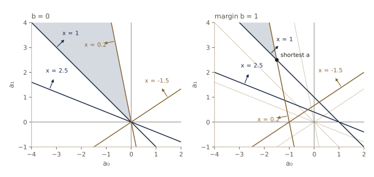
Think of \(\mathbf{a}\) as a point in weight space. Each normalized sample \(\mathbf{y}_i\) contributes a hyperplane \(\mathbf{a}^{t}\mathbf{y}_i = 0\), passing through the origin of the space and having \(\mathbf{y}_i\) as its normal, and a solution vector must lie on the positive side of every one of them. The intersection of these \(n\) half-spaces is the solution region; any vector inside it is a solution vector. Do not confuse it with a decision region: the solution region lives in weight space, the decision regions in feature space. It is a convex cone — if \(\mathbf{a}\) is a solution so is \(c\,\mathbf{a}\) for any \(c > 0\) — so solution vectors are never unique.
To pick a solution more likely to classify new samples well, we can ask for one toward the middle of the region. Two ways to say this: find the unit vector whose closest sample lies as far as possible from the separating plane, or find the shortest \(\mathbf{a}\) with
\[\mathbf{a}^{t}\mathbf{y}_i \ge b \quad \text{for all } i,\]where \(b > 0\) is a margin. The new region is the intersection of the half-spaces \(\mathbf{a}^{t}\mathbf{y}_i \ge b\); each of its walls is the old wall moved inward by \(b/\lVert \mathbf{y}_i \rVert\). Beyond improving the solution, a margin protects iterative procedures from creeping toward a limit that sits on the solution region’s edge, a danger we meet with relaxation.
A one-dimensional problem gives a two-dimensional weight space, small enough to draw. Our four samples are \(x = 1.0\) and \(2.5\) in \(\omega_1\) and \(x = -1.5\) and \(0.2\) in \(\omega_2\); the augmented vectors are \(\mathbf{y} = (1, x)^{t}\) and \(\mathbf{a} = (a_0, a_1)^{t}\). The next cell finds the angular extent of the solution cone by scanning directions, and the shortest vector in the margin region \(b = 1\) by a grid search.
x_w = np.array([1.0, 2.5, -1.5, 0.2])
lab_w = np.array([0, 0, 1, 1])
Y_w = normalize(augment(x_w[:, None]), lab_w)            # the four normalized samples
print("normalized samples:\n", Y_w)

theta = np.radians(np.linspace(-180, 180, 360001))
dirs = np.column_stack([np.cos(theta), np.sin(theta)])
inside = np.all(dirs @ Y_w.T > 0, axis=1)
print(f"solution cone: directions from {np.degrees(theta[inside].min()):.2f} "
      f"to {np.degrees(theta[inside].max()):.2f} degrees")

b = 1.0
ag = np.linspace(-4, 4, 801)
Ag = np.array(np.meshgrid(ag, ag)).reshape(2, -1).T
ok = np.all(Ag @ Y_w.T >= b - 1e-12, axis=1)
a_short = Ag[ok][np.argmin(np.linalg.norm(Ag[ok], axis=1))]
print(f"shortest a with a^t y_i >= 1: {a_short}, boundary at x = {-a_short[0] / a_short[1]:.3f}")
print("walls move inward by b/||y_i|| =", b / np.linalg.norm(Y_w, axis=1))
normalized samples:
 [[ 1.   1. ]
 [ 1.   2.5]
 [-1.   1.5]
 [-1.  -0.2]]
solution cone: directions from 101.31 to 135.00 degrees
shortest a with a^t y_i >= 1: [-1.5  2.5], boundary at x = 0.600
walls move inward by b/||y_i|| = [0.7071 0.3714 0.5547 0.9806]
The solution cone is bounded by the hyperplanes of the two samples nearest the class boundary, \(x = 1.0\) and \(x = 0.2\); the other two constraints are inactive. The shortest vector with margin 1 is \((-1.5, 2.5)^{t}\), which puts the decision point at \(x = 0.6\), exactly halfway between the two closest samples — our first glimpse of the maximum-margin idea behind support vector machines.
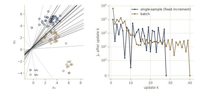
For most of the module we need a larger two-dimensional data set. We generate two classes on opposite sides of a line, keeping only points at least 0.3 from it so that the data are separable with a known margin, and shuffle the order in which the samples are stored. Class \(\omega_2\) has a main cloud and a small cluster far out on its own side; that cluster is harmless to a separating line but, as we will see, not to squared error.
w_gen = np.array([-1.7, -0.6, 1.0])                     # (w0, w1, w2) of the line used to generate the data

def sample_side(r, mean, sd, m, side, gap):
    """m Gaussian points lying on one side of the line w_gen, at least `gap` away from it."""
    out = np.empty((0, 2))
    while len(out) < m:
        X = r.normal(mean, sd, size=(4 * m, 2))
        dist = side * (augment(X) @ w_gen) / np.linalg.norm(w_gen[1:])    # signed distance
        out = np.vstack([out, X[dist > gap]])
    return out[:m]

def make_separable(seed, gap=0.3):
    r = np.random.default_rng(seed)
    X1 = sample_side(r, [3.0, 5.0], [1.2, 0.7], 40, +1, gap)     # omega_1
    X2 = sample_side(r, [3.0, 2.2], [1.2, 0.7], 30, -1, gap)     # omega_2, main cloud
    X2f = sample_side(r, [6.0, -3.0], [0.5, 0.5], 10, -1, gap)   # omega_2, far cluster
    X, labels = np.vstack([X1, X2, X2f]), np.r_[np.zeros(40, int), np.ones(40, int)]
    order = r.permutation(len(X))                                # present the classes interleaved
    return X[order], labels[order]

Xs, labs = make_separable(1)
Ys = normalize(augment(Xs), labs)                        # 80 normalized samples, d-hat = 3
print(Ys.shape, "  w_gen separates them:", bool(np.all(Ys @ w_gen > 0)))
(80, 3) w_gen separates them: True
Gradient descent procedures
To solve \(\mathbf{a}^{t}\mathbf{y}_i > 0\) we will define a criterion \(J(\mathbf{a})\) that is minimized by solution vectors and minimize it. The basic tool is gradient descent: start from some \(\mathbf{a}(1)\) and repeatedly step against the gradient,
\[\mathbf{a}(k+1) = \mathbf{a}(k) - \eta(k)\,\nabla J(\mathbf{a}(k)),\]where the positive learning rate \(\eta(k)\) sets the step size; stop when the step \(\eta(k)\nabla J\) becomes smaller than a threshold. The recurring difficulty is choosing \(\eta(k)\): too small and progress is slow, too large and the steps overshoot and can diverge.
A principled choice comes from a second-order model. Near \(\mathbf{a}(k)\),
\[J(\mathbf{a}) \approx J(\mathbf{a}(k)) + \nabla J^{t}(\mathbf{a} - \mathbf{a}(k)) + \frac{1}{2}(\mathbf{a} - \mathbf{a}(k))^{t}\mathbf{H}(\mathbf{a} - \mathbf{a}(k)),\]where \(\mathbf{H}\) is the Hessian, the matrix of second derivatives \(\partial^2 J/\partial a_i \partial a_j\) at \(\mathbf{a}(k)\). Substituting the gradient step gives a quadratic in \(\eta\),
\[J(\mathbf{a}(k+1)) \approx J(\mathbf{a}(k)) - \eta\lVert \nabla J \rVert^2 + \frac{1}{2}\eta^2\,\nabla J^{t}\mathbf{H}\,\nabla J ,\]and setting its derivative with respect to \(\eta\) to zero gives the best step along the gradient,
\[\eta(k) = \frac{\lVert \nabla J \rVert^2}{\nabla J^{t}\mathbf{H}\,\nabla J}.\]If \(J\) is quadratic, \(\mathbf{H}\) is constant and this is an exact line search. Instead of stepping along the gradient at all, we can jump to the minimum of the quadratic model: setting the model’s gradient \(\nabla J + \mathbf{H}(\mathbf{a} - \mathbf{a}(k))\) to zero gives Newton’s method,
\[\mathbf{a}(k+1) = \mathbf{a}(k) - \mathbf{H}^{-1}\nabla J .\]Newton usually gains much more per step, and on a quadratic criterion it lands on the minimum in one step. But it needs \(\mathbf{H}\) to be nonsingular and costs a linear solve, \(O(\hat{d}^3)\), per step, which on large problems can outweigh its advantage; it also needs care on nonquadratic criteria such as the error surfaces of module 06.
To compare the three, we minimize the squared-error criterion \(J_s(\mathbf{a}) = \lVert \mathbf{Y}\mathbf{a} - \mathbf{1} \rVert^2\) on our data (it is the subject of the MSE section; here it is just a convenient quadratic). Its gradient is \(2\mathbf{Y}^{t}(\mathbf{Y}\mathbf{a} - \mathbf{1})\) and its Hessian \(2\mathbf{Y}^{t}\mathbf{Y}\).
def J_s(a, Y, b):
    return np.sum((Y @ a - b) ** 2)

def grad_J_s(a, Y, b):
    return 2 * Y.T @ (Y @ a - b)

def descend(Y, b, step, tol=1e-8, max_iter=100000):
    """Gradient descent a <- a - eta(k) grad J; `step(grad)` returns eta(k). Returns (a, iterations)."""
    a = np.zeros(Y.shape[1])
    for k in range(1, max_iter + 1):
        grad = grad_J_s(a, Y, b)
        if np.linalg.norm(grad) < tol:
            return a, k - 1
        a = a - step(grad) * grad
    return a, max_iter

b1 = np.ones(len(Ys))
H = 2 * Ys.T @ Ys                                   # constant Hessian of J_s
lam = np.linalg.eigvalsh(H)
print(f"eigenvalues of H: {lam};  condition number {lam[-1] / lam[0]:.1f}")

a_fixed, it_fixed = descend(Ys, b1, lambda gr: 1.0 / lam[-1])
a_opt, it_opt = descend(Ys, b1, lambda gr: (gr @ gr) / (gr @ H @ gr))
a_newton = -np.linalg.solve(H, grad_J_s(np.zeros(3), Ys, b1))      # one Newton step from a = 0
print(f"fixed eta = 1/lambda_max: {it_fixed} iterations;  optimal eta(k): {it_opt} iterations")
print(f"Newton, one step: gradient norm {np.linalg.norm(grad_J_s(a_newton, Ys, b1)):.1e}, "
      f"distance to the others {np.linalg.norm(a_newton - a_opt):.1e}")

gr0 = grad_J_s(np.zeros(3), Ys, b1)                   # check the optimal step by a line search
etas = np.linspace(0, 2 * (gr0 @ gr0) / (gr0 @ H @ gr0), 20001)
best = etas[np.argmin([J_s(-e * gr0, Ys, b1) for e in etas])]
print(f"first step: formula eta = {(gr0 @ gr0) / (gr0 @ H @ gr0):.6f}, line search {best:.6f}")
eigenvalues of H: [   7.8342 1066.9374 3634.6664];  condition number 463.9
fixed eta = 1/lambda_max: 9668 iterations;  optimal eta(k): 4560 iterations
Newton, one step: gradient norm 3.0e-13, distance to the others 1.0e-09
first step: formula eta = 0.000538, line search 0.000538
The Hessian’s eigenvalues differ by a factor of more than 400 — the samples sit far from the origin, so the bias and the other weights are strongly coupled — and the criterion is a long, narrow valley. A fixed step small enough to be safe along the steep direction crawls along the shallow one; the optimal step per iteration helps but still zigzags across the valley; Newton’s method, which rescales every direction by its curvature, reaches the minimum in a single step. On large problems, though, a slightly-too-small fixed rate with a few more iterations is often cheaper overall than computing the optimal rate or the Newton step every time.
Minimizing the perceptron criterion function
The perceptron criterion
What should we minimize to solve \(\mathbf{a}^{t}\mathbf{y}_i > 0\)? The number of samples that \(\mathbf{a}\) misclassifies is the obvious choice and a poor one: it is piecewise constant, so its gradient is zero or undefined everywhere. The perceptron criterion replaces the count by a sum that grows with how badly each mistake is made:
\[J_p(\mathbf{a}) = \sum_{\mathbf{y} \in \mathcal{Y}(\mathbf{a})} \left(-\mathbf{a}^{t}\mathbf{y}\right),\]where \(\mathcal{Y}(\mathbf{a})\) is the set of samples misclassified by \(\mathbf{a}\), those with \(\mathbf{a}^{t}\mathbf{y} \le 0\) (if there are none, \(J_p = 0\)). Every term is nonnegative, so \(J_p \ge 0\), and \(J_p = 0\) exactly when \(\mathbf{a}\) is a solution vector or lies on the boundary of the solution region. Geometrically, \(-\mathbf{a}^{t}\mathbf{y}/\lVert \mathbf{a} \rVert\) is the distance from a misclassified \(\mathbf{y}\) to the hyperplane \(\mathbf{a}^{t}\mathbf{y} = 0\), so \(J_p\) is \(\lVert \mathbf{a} \rVert\) times the total distance of the misclassified samples from the decision boundary. Within any region of weight space where the misclassified set stays the same, \(J_p\) is linear, with gradient
\[\nabla J_p = \sum_{\mathbf{y} \in \mathcal{Y}(\mathbf{a})} (-\mathbf{y}),\]so gradient descent gives the update
\[\mathbf{a}(k+1) = \mathbf{a}(k) + \eta(k) \sum_{\mathbf{y} \in \mathcal{Y}_k} \mathbf{y},\]where \(\mathcal{Y}_k\) is the set of samples misclassified by \(\mathbf{a}(k)\). This is the batch perceptron: add a multiple of the sum of the misclassified samples to the weight vector, and repeat until nothing is misclassified. “Batch” means that each update uses a whole group of samples; the single-sample rules below update after every mistake.
def J_p(a, Y):
    """Perceptron criterion: sum of -a^t y over the samples with a^t y <= 0."""
    s = Y @ a
    return -np.sum(s[s <= 0])

def grad_J_p(a, Y):
    return -Y[Y @ a <= 0].sum(axis=0)

def batch_perceptron(Y, eta=lambda k: 1.0, a=None, max_iter=100000):
    """a <- a + eta(k) * (sum of the misclassified y). Returns (a, number of updates)."""
    a = np.zeros(Y.shape[1]) if a is None else np.array(a, float)
    for k in range(1, max_iter + 1):
        mis = Y @ a <= 0
        if not mis.any():
            return a, k - 1
        a = a + eta(k) * Y[mis].sum(axis=0)
    return a, None

a_batch, n_batch = batch_perceptron(Ys)
print(f"batch perceptron: {n_batch} updates, a = {a_batch}, "
      f"misclassified: {np.sum(Ys @ a_batch <= 0)}")

a_chk, h = np.array([0.3, -0.2, 0.5]), 1e-6          # finite-difference check of the gradient
num = [(J_p(a_chk + h * e, Ys) - J_p(a_chk - h * e, Ys)) / (2 * h) for e in np.eye(3)]
print("gradient:", grad_J_p(a_chk, Ys), " finite differences:", np.array(num))
batch perceptron: 40 updates, a = [ -66.     -125.3012  130.6631], misclassified: 0
gradient: [29.     90.0892 62.5081]  finite differences: [29.     90.0892 62.5081]
Starting from \(\mathbf{a} = \mathbf{0}\) (where every sample counts as misclassified, since \(\mathbf{a}^{t}\mathbf{y} = 0\)), a handful of batch updates reaches a separating vector. We keep a_batch as a known solution vector for the checks below.
Convergence proof for single-sample correction
The batch rule is harder to analyze than a variant that looks at one sample at a time. Present the samples in a sequence in which each one keeps recurring forever — cycling through them is the easy way — and change \(\mathbf{a}\) only when the current sample is misclassified. With a constant learning rate, \(\eta\) merely rescales \(\mathbf{a}\), so we may take \(\eta = 1\); this is the fixed-increment case. Since only mistakes matter, write \(\mathbf{y}^1, \mathbf{y}^2, \dots\) (superscripts) for the sequence of samples that triggered corrections; each \(\mathbf{y}^k\) is one of the \(\mathbf{y}_i\), possibly repeated. The fixed-increment rule is then
\[\mathbf{a}(1) \text{ arbitrary}, \qquad \mathbf{a}(k+1) = \mathbf{a}(k) + \mathbf{y}^k, \qquad \text{where } \mathbf{a}(k)^{t}\mathbf{y}^k \le 0 .\]In weight space, \(\mathbf{a}(k)\) is on the wrong side (or on) the hyperplane \(\mathbf{a}^{t}\mathbf{y}^k = 0\), and adding \(\mathbf{y}^k\), the hyperplane’s normal, moves it toward that hyperplane and perhaps across. Either way the inner product improves by exactly \(\lVert \mathbf{y}^k \rVert^2\): \(\mathbf{a}(k+1)^{t}\mathbf{y}^k = \mathbf{a}(k)^{t}\mathbf{y}^k + \lVert \mathbf{y}^k \rVert^2\). The rule can only stop if the samples are linearly separable. The converse is the main theorem of this section.
Result (perceptron convergence). If the samples are linearly separable, the fixed-increment rule makes only finitely many corrections, and it stops at a solution vector. Starting from \(\mathbf{a}(1) = \mathbf{0}\), the number of corrections is at most
\[k_0 = \frac{\beta^2 \lVert \hat{\mathbf{a}} \rVert^2}{\gamma^2}, \qquad \beta^2 = \max_i \lVert \mathbf{y}_i \rVert^2, \qquad \gamma = \min_i \hat{\mathbf{a}}^{t}\mathbf{y}_i > 0,\]where \(\hat{\mathbf{a}}\) is any solution vector.
Proof. A natural first attempt is to show that every correction brings \(\mathbf{a}(k)\) closer to some solution vector \(\hat{\mathbf{a}}\). That is false in general — we will see a correction move away from \(\hat{\mathbf{a}}\) in the next cell — but it becomes true if we aim at a sufficiently long solution vector \(\alpha\hat{\mathbf{a}}\), \(\alpha > 0\).
Subtract \(\alpha\hat{\mathbf{a}}\) from both sides of the update and take squared lengths:
\[\lVert \mathbf{a}(k+1) - \alpha\hat{\mathbf{a}} \rVert^2 = \lVert \mathbf{a}(k) - \alpha\hat{\mathbf{a}} \rVert^2 + 2\,\mathbf{a}(k)^{t}\mathbf{y}^k - 2\alpha\,\hat{\mathbf{a}}^{t}\mathbf{y}^k + \lVert \mathbf{y}^k \rVert^2 .\]Bound the three new terms one at a time. The first is at most zero because \(\mathbf{y}^k\) was misclassified. The second is at most \(-2\alpha\gamma\) because \(\hat{\mathbf{a}}^{t}\mathbf{y}^k \ge \gamma\). The third is at most \(\beta^2\). So
\[\lVert \mathbf{a}(k+1) - \alpha\hat{\mathbf{a}} \rVert^2 \le \lVert \mathbf{a}(k) - \alpha\hat{\mathbf{a}} \rVert^2 - 2\alpha\gamma + \beta^2 .\]Now choose \(\alpha = \beta^2/\gamma\), which makes \(-2\alpha\gamma + \beta^2 = -\beta^2\): every correction reduces the squared distance to \(\alpha\hat{\mathbf{a}}\) by at least \(\beta^2\). After \(k\) corrections,
\[0 \le \lVert \mathbf{a}(k+1) - \alpha\hat{\mathbf{a}} \rVert^2 \le \lVert \mathbf{a}(1) - \alpha\hat{\mathbf{a}} \rVert^2 - k\beta^2 ,\]so \(k\) can never exceed \(\lVert \mathbf{a}(1) - \alpha\hat{\mathbf{a}} \rVert^2/\beta^2\). With \(\mathbf{a}(1) = \mathbf{0}\) this is \(\alpha^2\lVert \hat{\mathbf{a}} \rVert^2/\beta^2 = \beta^2\lVert \hat{\mathbf{a}} \rVert^2/\gamma^2\). Finally, once corrections stop, every sample — each of which keeps appearing in the sequence — must be classified correctly, so the final vector is a solution. \(\square\)
The bound has a clean reading. \(\gamma/\lVert \hat{\mathbf{a}} \rVert\) is the smallest distance from a sample to the hyperplane \(\hat{\mathbf{a}}^{t}\mathbf{y} = 0\) in augmented space (the margin of \(\hat{\mathbf{a}}\)), and \(\beta\) is the radius of a ball holding all the samples, so \(k_0 = (\beta / \text{margin})^2\) — the form of the bound in Intro to ML, module 04. The best bound uses the solution with the largest margin. Hard problems are those where every solution vector is nearly orthogonal to some sample. Unfortunately the bound cannot be computed before the problem is solved, since it depends on an unknown \(\hat{\mathbf{a}}\).
def fixed_increment(Y, a=None, max_passes=10000):
    """Single-sample fixed-increment rule, cycling through the samples.
    Returns (a, indices of the corrected samples, path of weight vectors, passes used or None)."""
    a = np.zeros(Y.shape[1]) if a is None else np.array(a, float)
    path, corrected = [a.copy()], []
    for p in range(1, max_passes + 1):
        changed = False
        for i, y in enumerate(Y):
            if a @ y <= 0:                     # misclassified (or on the boundary)
                a = a + y                      # a(k+1) = a(k) + y^k
                corrected.append(i)
                path.append(a.copy())
                changed = True
        if not changed:
            return a, np.array(corrected), np.array(path), p
    return a, np.array(corrected), np.array(path), None

a_fi, corr_fi, path_fi, passes_fi = fixed_increment(Ys)
print(f"fixed increment: {len(corr_fi)} corrections in {passes_fi} passes; "
      f"errors now {np.sum(Ys @ a_fi <= 0)}")

a_hat = a_batch                                            # any solution vector will do
beta2 = np.max(np.sum(Ys**2, axis=1))
gamma = np.min(Ys @ a_hat)
alpha = beta2 / gamma
drop = -np.diff(np.sum((path_fi - alpha * a_hat) ** 2, axis=1))    # decrease per correction
print(f"decrease of ||a(k) - alpha a_hat||^2 per correction: min {drop.min():.2f} >= beta^2 = {beta2:.2f}")
d_plain = np.linalg.norm(path_fi - a_hat, axis=1)
print(f"corrections that moved a(k) farther from a_hat itself: {np.sum(np.diff(d_plain) > 0)}")
print(f"bound k0 = beta^2 ||a_hat||^2 / gamma^2 = {beta2 * (a_hat @ a_hat) / gamma**2:.0f}")
fixed increment: 28 corrections in 4 passes; errors now 0
decrease of ||a(k) - alpha a_hat||^2 per correction: min 65.23 >= beta^2 = 54.27
corrections that moved a(k) farther from a_hat itself: 2
bound k0 = beta^2 ||a_hat||^2 / gamma^2 = 574960705
The squared distance to \(\alpha\hat{\mathbf{a}}\) drops by at least \(\beta^2\) at every correction, as the proof promises, while the distance to \(\hat{\mathbf{a}}\) itself goes up at two of the steps. The bound is loose — it is a worst case over all data sets with the same \(\beta\) and \(\gamma\), and our \(\hat{\mathbf{a}}\) is far from the largest-margin solution — but its dependence on the margin is real. To see it, the next cell adds four samples at distance gap from the generating line, two on each side and far apart along it, so that every separating line must thread between them; as gap shrinks, the solution region becomes a thinner and thinner cone. The cell also applies the rule to the \(\varphi\)-mapped ring data of the previous section.
n_hat = w_gen[1:] / np.linalg.norm(w_gen[1:])             # unit normal of the generating line
u_line = np.array([n_hat[1], -n_hat[0]])                   # unit vector along it
x_line = -w_gen[0] * w_gen[1:] / (w_gen[1:] @ w_gen[1:])   # a point on it
for gap in [0.3, 0.1, 0.03]:
    X_hard = np.array([x_line + s * 3 * u_line + side * gap * n_hat
                       for side in (+1, -1) for s in (+1, -1)])       # two omega_1, then two omega_2
    Y_gap = normalize(augment(np.vstack([Xs, X_hard])), np.r_[labs, 0, 0, 1, 1])
    a_g, corr_g, _, p_g = fixed_increment(Y_gap)
    print(f"gap {gap:4.2f}: {len(corr_g):5d} corrections, {p_g:4d} passes")

a_ring, corr_ring, _, p_ring = fixed_increment(normalize(quad_features(X_ring), lab_ring))
print(f"ring data, quadratic features: {len(corr_ring)} corrections in {p_ring} passes")
print("a =", a_ring)
gap 0.30:    31 corrections,    4 passes
gap 0.10:   292 corrections,  103 passes
gap 0.03:  7283 corrections, 3218 passes
ring data, quadratic features: 12 corrections in 5 passes
a = [-4.     -0.5221  0.4916  3.4769 -1.108   3.4854]
Each threefold reduction of the gap multiplies the number of corrections by roughly ten or more, in line with the \(1/\gamma^2\) in the bound. On the ring data the perceptron finds a quadratic boundary quickly. The coefficients of \(x_1^2\) and \(x_2^2\) are nearly equal and the cross term is about a third of their size, so the boundary is a slightly tilted ellipse around the inner disk, not the circle we would have drawn by hand; the perceptron stops at the first boundary that works.
Some direct generalizations
The fixed-increment rule is the simplest of many rules for linear inequalities. Two generalizations matter most.
The variable-increment rule with margin uses a learning rate \(\eta(k)\) and corrects whenever \(\mathbf{a}(k)^{t}\mathbf{y}^k\) fails to exceed a margin \(b \ge 0\):
\[\mathbf{a}(k+1) = \mathbf{a}(k) + \eta(k)\,\mathbf{y}^k, \qquad \text{where } \mathbf{a}(k)^{t}\mathbf{y}^k \le b .\]If the samples are linearly separable and
\[\eta(k) \ge 0, \qquad \sum_{k=1}^{m}\eta(k) \to \infty, \qquad \frac{\sum_{k=1}^{m}\eta^2(k)}{\left(\sum_{k=1}^{m}\eta(k)\right)^2} \to 0 \qquad (m \to \infty),\]then \(\mathbf{a}(k)\) converges to a solution with \(\mathbf{a}^{t}\mathbf{y}_i > b\) for all \(i\) (DHS Problem 19 asks for the proof; it follows the pattern of the one above, tracking the squared distance to a scaled solution vector). A constant \(\eta\) satisfies the conditions, and so does \(\eta(k) = 1/k\) or \(1/\sqrt{k}\).
The batch variable-increment rule is gradient descent on \(J_p\) with a variable rate, the batch perceptron above with \(\eta(k)\) in front of the sum. Its convergence follows from the single-sample result by one observation: if \(\hat{\mathbf{a}}\) separates the samples, it also classifies correctly any sum of samples, \(\hat{\mathbf{a}}^{t}\sum_{\mathbf{y} \in \mathcal{Y}_k}\mathbf{y} > 0\). So the batch rule is the single-sample rule applied to a sequence of separable “correction vectors”. Summing over all mistakes smooths the path of the weight vector: sample-to-sample fluctuations tend to cancel while the systematic direction adds up.
def variable_increment(Y, b=0.0, eta=lambda k: 1.0, a=None, max_passes=10000):
    """Single-sample rule with margin: when a^t y^k <= b, a <- a + eta(k) y^k (k counts corrections)."""
    a = np.zeros(Y.shape[1]) if a is None else np.array(a, float)
    k = 0
    for p in range(1, max_passes + 1):
        changed = False
        for y in Y:
            if a @ y <= b:
                k += 1
                a = a + eta(k) * y
                changed = True
        if not changed:
            return a, k, p
    return a, k, None

for b, name, eta in [(0.0, "1", lambda k: 1.0), (1.0, "1", lambda k: 1.0),
                     (10.0, "1", lambda k: 1.0), (1.0, "1/sqrt(k)", lambda k: k ** -0.5)]:
    a_v, k_v, p_v = variable_increment(Ys, b, eta)
    dist = Ys @ a_v / np.linalg.norm(a_v[1:])       # x-space distances of the samples to the boundary
    print(f"b = {b:4.1f}, eta = {name:9s}: {k_v:4d} corrections, min a^t y = {np.min(Ys @ a_v):6.2f}, "
          f"closest sample {dist.min():.3f}")

print(f"a_hat^t (sum of samples misclassified by a = 0) = {a_hat @ Ys.sum(axis=0):.2f} > 0")
for name, eta in [("1", lambda k: 1.0), ("k", lambda k: float(k)), ("1/k", lambda k: 1.0 / k)]:
    n_up = batch_perceptron(Ys, eta)[1]
    print(f"batch rule with eta(k) = {name:3s}: " +
          (f"{n_up} updates" if n_up is not None else "not converged after 100000 updates"))
b =  0.0, eta = 1        :   28 corrections, min a^t y =   0.21, closest sample 0.013
b =  1.0, eta = 1        :   46 corrections, min a^t y =   1.00, closest sample 0.076
b = 10.0, eta = 1        :  224 corrections, min a^t y =  10.57, closest sample 0.205
b =  1.0, eta = 1/sqrt(k):  157 corrections, min a^t y =   1.20, closest sample 0.187
a_hat^t (sum of samples misclassified by a = 0) = 26438.13 > 0
batch rule with eta(k) = 1  : 40 updates
batch rule with eta(k) = k  : 54 updates
batch rule with eta(k) = 1/k: not converged after 100000 updates
A larger margin costs more corrections but pushes the samples farther from the boundary, a crude version of looking for a solution in the middle of the solution region. The batch rule converges even with a learning rate that grows like \(k\), a curiosity of the separable case. With \(\eta(k) = 1/k\) it is guaranteed to converge too, yet it does not get there in 100,000 updates: the first update adds the sum of all 80 samples, a long vector, and the later steps shrink so fast that their total length grows only like \(\ln k\). The theorem promises a finite number of steps, not a practical one. On data that are not separable, on the other hand, we do want \(\eta(k)\) to shrink, so that a few troublesome samples cannot keep throwing the weights around. In practice the choices of \(\eta\), \(b\), and the scaling of the features all matter. A useful rule of thumb for the margin is to make \(b\) comparable to \(\eta\lVert \mathbf{y}^k \rVert^2\), the amount one correction adds to \(\mathbf{a}^{t}\mathbf{y}^k\): much smaller and the margin has no effect, much larger and many corrections are needed.
Winnow. A close relative of the perceptron updates its weights by multiplication instead of addition. In the balanced Winnow algorithm there are two nonnegative weight vectors, \(\mathbf{a}^{+}\) for \(\omega_1\) and \(\mathbf{a}^{-}\) for \(\omega_2\), and the classifier is the sign of \((\mathbf{a}^{+} - \mathbf{a}^{-})^{t}\mathbf{y}\). On a mistake with a sample of \(\omega_1\) (\(z = +1\)) each \(a_i^{+}\) is multiplied by \(\alpha^{y_i}\) and each \(a_i^{-}\) by \(\alpha^{-y_i}\), for a fixed \(\alpha > 1\); a mistake on \(\omega_2\) (\(z = -1\)) does the reverse. Winnow has its own convergence theory, more intricate than the perceptron’s, and its multiplicative updates shine when most features are irrelevant: for simple targets such as a disjunction of a few features, its number of mistakes grows only with the logarithm of the number of features. We test that on an online stream of sparse binary feature vectors labeled \(\omega_1\) when any of the first 3 of the \(d\) features is on; the other features are irrelevant.
def balanced_winnow_mistakes(Y, z, alpha=2.0):
    """One online pass of balanced Winnow; Y has entries in {0, 1} (with y_0 = 1), z in {+1, -1}."""
    a_pos, a_neg = np.ones(Y.shape[1]), np.ones(Y.shape[1])
    mistakes = 0
    for y, zk in zip(Y, z):
        if np.sign((a_pos - a_neg) @ y) != zk:
            mistakes += 1
            a_pos *= alpha ** (zk * y)
            a_neg *= alpha ** (-zk * y)
    return mistakes

def perceptron_mistakes(Y, z):
    """One online pass of the fixed-increment rule on the normalized samples z y."""
    a, mistakes = np.zeros(Y.shape[1]), 0
    for y in z[:, None] * Y:
        if a @ y <= 0:
            a, mistakes = a + y, mistakes + 1
    return mistakes

rng_w = np.random.default_rng(31)
for d in [20, 200, 2000]:
    Xb = (rng_w.uniform(size=(3000, d)) < 0.1).astype(float)          # sparse binary features
    Xb[:, :3] = rng_w.uniform(size=(3000, 3)) < 0.3                     # the three relevant ones
    zb = np.where(Xb[:, :3].sum(axis=1) >= 1, 1, -1)                    # omega_1: any of the three on
    Yb = augment(Xb)
    print(f"d = {d:4d}: mistakes in 3000 samples - perceptron {perceptron_mistakes(Yb, zb):4d}, "
          f"balanced Winnow {balanced_winnow_mistakes(Yb, zb):3d}")
d =   20: mistakes in 3000 samples - perceptron   32, balanced Winnow  22
d =  200: mistakes in 3000 samples - perceptron  161, balanced Winnow  47
d = 2000: mistakes in 3000 samples - perceptron  662, balanced Winnow  59
The perceptron’s mistakes grow twentyfold as \(d\) grows a hundredfold, while Winnow’s less than triple. (DHS Computer exercise 6 explores this further.)
Relaxation procedures
The perceptron criterion is one member of a family. Replacing it by other functions of the misclassified samples, and descending on them, gives the relaxation procedures.
The descent algorithm
A close relative of \(J_p\) squares each term:
\[J_q(\mathbf{a}) = \sum_{\mathbf{y} \in \mathcal{Y}(\mathbf{a})} (\mathbf{a}^{t}\mathbf{y})^2 .\]Its gradient is continuous where that of \(J_p\) jumps, so it presents a smoother surface. It has two defects. Near the edge of the solution region it is so flat that descent can end up converging to an edge point — the worst case being \(\mathbf{a} = \mathbf{0}\), which minimizes \(J_q\) trivially. And the longest samples can dominate its value. Both are cured by a margin and a normalization:
\[J_r(\mathbf{a}) = \frac{1}{2}\sum_{\mathbf{y} \in \mathcal{Y}(\mathbf{a})} \frac{(\mathbf{a}^{t}\mathbf{y} - b)^2}{\lVert \mathbf{y} \rVert^2},\]where now \(\mathcal{Y}(\mathbf{a})\) is the set of samples with \(\mathbf{a}^{t}\mathbf{y} \le b\). \(J_r\) is never negative, and it is zero exactly when \(\mathbf{a}^{t}\mathbf{y} \ge b\) for every sample. Its gradient is \(\nabla J_r = \sum_{\mathcal{Y}} \frac{\mathbf{a}^{t}\mathbf{y} - b}{\lVert \mathbf{y} \rVert^2}\mathbf{y}\), which gives the batch relaxation rule with margin
\[\mathbf{a}(k+1) = \mathbf{a}(k) + \eta(k)\sum_{\mathbf{y} \in \mathcal{Y}_k}\frac{b - \mathbf{a}(k)^{t}\mathbf{y}}{\lVert \mathbf{y} \rVert^2}\,\mathbf{y},\]and, one sample at a time with a fixed \(\eta\), the single-sample relaxation rule with margin
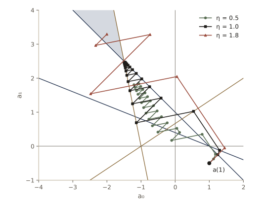
\[\mathbf{a}(k+1) = \mathbf{a}(k) + \eta\,\frac{b - \mathbf{a}(k)^{t}\mathbf{y}^k}{\lVert \mathbf{y}^k \rVert^2}\,\mathbf{y}^k, \qquad \text{where } \mathbf{a}(k)^{t}\mathbf{y}^k \le b .\]The single-sample rule has a clear geometric meaning. The distance from \(\mathbf{a}(k)\) to the hyperplane \(\mathbf{a}^{t}\mathbf{y}^k = b\) is \((b - \mathbf{a}(k)^{t}\mathbf{y}^k)/\lVert \mathbf{y}^k \rVert\), and \(\mathbf{y}^k/\lVert \mathbf{y}^k \rVert\) is that hyperplane’s unit normal, so the rule moves \(\mathbf{a}(k)\) a fraction \(\eta\) of the way to the hyperplane. With \(\eta = 1\) it lands exactly on the hyperplane, “relaxing” the violated constraint. Multiplying the update by \(\mathbf{y}^{k\,t}\),
\[\mathbf{a}(k+1)^{t}\mathbf{y}^k - b = (1 - \eta)\left(\mathbf{a}(k)^{t}\mathbf{y}^k - b\right),\]so with \(\eta < 1\) (underrelaxation) the constraint is still violated after the step, and with \(\eta > 1\) (overrelaxation) it is overshot and satisfied. We restrict \(\eta\) to \(0 < \eta < 2\).
Convergence proof
On separable samples the relaxation rule may make infinitely many corrections: with \(\eta \le 1\) it approaches each violated hyperplane without ever getting past it. What we can prove is that it still gets where we want to go.
Result (relaxation). Let the samples be linearly separable, \(b > 0\), and \(0 < \eta < 2\). Then the single-sample relaxation rule either stops at a vector with \(\mathbf{a}^{t}\mathbf{y}_i \ge b\) for all \(i\), or produces an infinite sequence that converges to a point on the boundary of that region. In either case, after finitely many corrections every \(\mathbf{a}(k)\) is a solution vector.
Proof. Let \(\hat{\mathbf{a}}\) be any vector with \(\hat{\mathbf{a}}^{t}\mathbf{y}_i \ge b\) for all \(i\) (it exists: scale up any separating vector), and write \(\delta_k = b - \mathbf{a}(k)^{t}\mathbf{y}^k \ge 0\) for the violation being corrected. Expanding the squared distance to \(\hat{\mathbf{a}}\) after the update,
\[\lVert \mathbf{a}(k+1) - \hat{\mathbf{a}} \rVert^2 = \lVert \mathbf{a}(k) - \hat{\mathbf{a}} \rVert^2 - 2\eta\,\frac{\delta_k}{\lVert \mathbf{y}^k \rVert^2}(\hat{\mathbf{a}} - \mathbf{a}(k))^{t}\mathbf{y}^k + \eta^2\frac{\delta_k^2}{\lVert \mathbf{y}^k \rVert^2}.\]Since \(\hat{\mathbf{a}}^{t}\mathbf{y}^k \ge b\), we have \((\hat{\mathbf{a}} - \mathbf{a}(k))^{t}\mathbf{y}^k \ge b - \mathbf{a}(k)^{t}\mathbf{y}^k = \delta_k\), and so
\[\lVert \mathbf{a}(k+1) - \hat{\mathbf{a}} \rVert^2 \le \lVert \mathbf{a}(k) - \hat{\mathbf{a}} \rVert^2 - \eta(2 - \eta)\frac{\delta_k^2}{\lVert \mathbf{y}^k \rVert^2}.\]With \(0 < \eta < 2\) the last term is negative: every correction brings \(\mathbf{a}(k)\) closer to every such \(\hat{\mathbf{a}}\), whichever one we pick. Two consequences follow. First, the sequence stays bounded. Second, summing the inequality over all corrections, \(\eta(2-\eta)\sum_k \delta_k^2/\lVert \mathbf{y}^k \rVert^2 \le \lVert \mathbf{a}(1) - \hat{\mathbf{a}} \rVert^2 < \infty\), so if there are infinitely many corrections then \(\delta_k \to 0\) and the step lengths \(\eta\delta_k/\lVert \mathbf{y}^k \rVert\) shrink to zero.
Now use the cycling. Within one pass through the \(n\) samples the weight vector moves by at most the sum of \(n\) steps, which tends to zero. When a sample is checked, either \(\mathbf{a}^{t}\mathbf{y}_i > b\) (no correction) or \(\mathbf{a}^{t}\mathbf{y}_i = b - \delta\) with \(\delta \to 0\). So in late passes every \(\mathbf{a}(k)\) satisfies \(\mathbf{a}(k)^{t}\mathbf{y}_i \ge b - \epsilon\) for all \(i\), with \(\epsilon \to 0\); since \(b > 0\), eventually all \(\mathbf{a}(k)^{t}\mathbf{y}_i > 0\). DHS §5.6.2 completes the picture with a neat geometric argument: the limit of \(\lVert \mathbf{a}(k) - \hat{\mathbf{a}} \rVert\) exists for every \(\hat{\mathbf{a}}\) in a region with nonempty interior, and only one point can have prescribed distances to all of them, so \(\mathbf{a}(k)\) converges to a single point, which must lie on the boundary of the margin region. \(\square\)
This is where the margin earns its keep: without it (\(b = 0\)) the limit could be a boundary point of the solution region itself, which is not a solution vector, possibly even \(\mathbf{a} = \mathbf{0}\).
def relaxation(Y, b, eta, a=None, max_passes=2000):
    """Single-sample relaxation with margin. Stops at the end of the first pass after which all a^t y_i > 0.
    Returns (a, path of weight vectors, list of (y index, delta_k), passes used or None)."""
    a = np.zeros(Y.shape[1]) if a is None else np.array(a, float)
    path, steps = [a.copy()], []
    for p in range(1, max_passes + 1):
        for i, y in enumerate(Y):
            delta = b - a @ y
            if delta > 0:                           # a^t y < b: correct (a^t y = b: zero step)
                a = a + eta * delta / (y @ y) * y            # move a fraction eta toward a^t y = b
                path.append(a.copy())
                steps.append((i, delta))
        if np.all(Y @ a > 0):
            return a, np.array(path), steps, p
    return a, np.array(path), steps, None

b_r = 1.0
a_hat_r = a_batch * b_r / np.min(Ys @ a_batch)             # a vector with a_hat^t y_i >= b for all i
for eta in [0.5, 1.0, 1.5, 1.9]:
    a_r, path_r, steps_r, p_r = relaxation(Ys, b_r, eta)
    d2 = np.sum((path_r - a_hat_r) ** 2, axis=1)
    promised = np.array([eta * (2 - eta) * dl**2 / (Ys[i] @ Ys[i]) for i, dl in steps_r])
    slack = np.min(-np.diff(d2) - promised)                  # >= 0 if the inequality holds
    print(f"eta = {eta}: {p_r:3d} passes, {len(steps_r):4d} corrections, "
          f"min a^t y / b = {np.min(Ys @ a_r) / b_r:.3f}, slack >= {slack:.0e}")

a_22, path_22, _, p_22 = relaxation(Ys, b_r, 2.2, max_passes=300)
print(f"eta = 2.2: corrections that moved a(k) away from a_hat: "
      f"{np.sum(np.diff(np.linalg.norm(path_22 - a_hat_r, axis=1)) > 0)}")
eta = 0.5:  19 passes,  462 corrections, min a^t y / b = 0.008, slack >= -5e-09
eta = 1.0:   9 passes,  180 corrections, min a^t y / b = 0.057, slack >= -3e-09
eta = 1.5:   6 passes,  104 corrections, min a^t y / b = 0.094, slack >= -2e-09
eta = 1.9:   4 passes,   62 corrections, min a^t y / b = 0.061, slack >= -3e-09
eta = 2.2: corrections that moved a(k) away from a_hat: 4
For every \(\eta\) in \((0, 2)\) the rule reaches a separating vector, and the distance to \(\hat{\mathbf{a}}\) falls by at least the promised amount at every correction (the slack is zero or positive up to rounding error; the squared distances themselves are about \(10^7\)). When we stop, as soon as the vector separates, the smallest \(\mathbf{a}^{t}\mathbf{y}_i\) is still well below \(b\): the sequence approaches the margin region from outside, and the margin’s job was only to pull it far enough to cross into the solution region. Overrelaxation needs the fewest corrections here. Beyond \(\eta = 2\) the proof’s key inequality fails: with \(\eta = 2.2\) some corrections move \(\mathbf{a}(k)\) away from \(\hat{\mathbf{a}}\), and although this run happens to finish, nothing guarantees that it will.
Nonseparable behavior
The perceptron and relaxation rules are error-correcting procedures: they change the weights when, and only when, a sample is misclassified (or violates the margin). That relentless search for zero errors is what makes them succeed on separable data. It also means that on data that are not separable they never stop.
And most real data sets are not separable. A set with fewer samples than twice the number of weights is more likely than not to be separable just by chance — we verify this in the linear-programming section — so to make training performance a reliable guide to test performance we need several times more samples than weights. Sets that large are almost never linearly separable, so how these procedures behave without separability matters in practice.
Each rule then produces an endless sequence of weight vectors, any of which may or may not be a good classifier. A few facts are known. For the fixed-increment rule, the length of \(\mathbf{a}(k)\) stays bounded, fluctuating around a limiting size, which suggests stopping once it settles; with integer-valued features the rule is a finite-state process that eventually cycles. Averaging the weight vectors over many corrections reduces the risk of stopping at an unlucky moment. A learning rate that decreases to zero, such as \(\eta(k) = \eta(1)/k\), damps the effect of the samples that make the set nonseparable; the rate matters, since shrinking too slowly leaves the weights sensitive to those samples and shrinking too fast freezes them before they are good. Our nonseparable data set has two overlapping Gaussian classes.
rng_ns = np.random.default_rng(8)
Xn = np.vstack([rng_ns.normal([0.0, 1.0], 1.0, size=(50, 2)),
                rng_ns.normal([1.5, -0.5], 1.0, size=(50, 2))])
labn = np.repeat([0, 1], 50)
Yn = normalize(augment(Xn), labn)

a_ns, corr_ns, path_ns, done_ns = fixed_increment(Yn, max_passes=300)
errs = np.sum(path_ns @ Yn.T <= 0, axis=1)                # training errors of every a(k) on the path
norms = np.linalg.norm(path_ns, axis=1)
late = slice(len(path_ns) // 2, None)
print(f"stopped by itself: {done_ns is not None};  {len(corr_ns)} corrections in 300 passes")
print(f"second half of the run: ||a(k)|| between {norms[late].min():.1f} and {norms[late].max():.1f}; "
      f"errors between {errs[late].min()} and {errs[late].max()}")
a_avg = path_ns[late].mean(axis=0)
print(f"errors: last a(k) {np.sum(Yn @ a_ns <= 0)}, average of the second half {np.sum(Yn @ a_avg <= 0)}, "
      f"best a(k) seen {errs.min()}")
for b, name, eta in [(0.0, "1/k", lambda k: 1.0 / k), (1.0, "1", lambda k: 1.0),
                     (1.0, "1/k", lambda k: 1.0 / k), (1.0, "1/sqrt(k)", lambda k: k ** -0.5)]:
    a_v, k_v, _ = variable_increment(Yn, b, eta, max_passes=300)
    print(f"margin b = {b}, eta(k) = {name:9s}: ||a|| = {np.linalg.norm(a_v):7.4f}, "
          f"errors {np.sum(Yn @ a_v <= 0)}")
stopped by itself: False;  2800 corrections in 300 passes
second half of the run: ||a(k)|| between 1.5 and 4.7; errors between 15 and 50
errors: last a(k) 32, average of the second half 21, best a(k) seen 15
margin b = 0.0, eta(k) = 1/k      : ||a|| =  0.0008, errors 49
margin b = 1.0, eta(k) = 1        : ||a|| =  4.5039, errors 38
margin b = 1.0, eta(k) = 1/k      : ||a|| =  1.9044, errors 20
margin b = 1.0, eta(k) = 1/sqrt(k): ||a|| =  1.7900, errors 18
The weight vector keeps moving forever, its length confined to a band, and its training error jumps between 15 and 50 from one correction to the next. Stopping at an arbitrary moment gives an arbitrary classifier; averaging the late weight vectors gives a steadier one.
The last four lines hold a warning and a remedy. A decreasing learning rate with no margin drives \(\mathbf{a}\) toward \(\mathbf{0}\): on nonseparable data the smallest value of \(J_p\) is \(J_p(\mathbf{0}) = 0\), so the descent heads for the useless zero vector; here \(\lVert \mathbf{a} \rVert\) has shrunk below 0.001 and the classifier gets half the samples wrong. With a margin \(b = 1\) the zero vector is no longer a minimizer; a constant rate still wanders, while a decaying rate settles on a reasonable classifier and stays there. The next section takes a different approach: give up on the guarantee of finding a separating vector, in exchange for a criterion that behaves well whether or not the data are separable.
Minimum squared-error procedures
The criteria so far look only at misclassified samples. The minimum squared-error (MSE) approach looks at all of them. Instead of asking for \(\mathbf{a}^{t}\mathbf{y}_i > 0\), it asks for \(\mathbf{a}^{t}\mathbf{y}_i = b_i\), where the \(b_i\) are positive constants we choose. We trade a system of linear inequalities for a more demanding but much better understood system of linear equations, and we give up the promise of a separating vector in return for an answer that is sensible whether or not the data are separable.
Minimum squared error and the pseudoinverse
Stack the normalized augmented samples as the rows of the \(n \times \hat{d}\) matrix \(\mathbf{Y}\) and the targets into the margin vector \(\mathbf{b} = (b_1, \dots, b_n)^{t}\). We want \(\mathbf{Y}\mathbf{a} = \mathbf{b}\). With more equations than unknowns (\(n > \hat{d}\), the usual case) there is typically no exact solution, so we minimize the squared norm of the error vector \(\mathbf{e} = \mathbf{Y}\mathbf{a} - \mathbf{b}\):
\[J_s(\mathbf{a}) = \lVert \mathbf{Y}\mathbf{a} - \mathbf{b} \rVert^2 = \sum_{i=1}^{n} (\mathbf{a}^{t}\mathbf{y}_i - b_i)^2 .\]The gradient is \(\nabla J_s = 2\mathbf{Y}^{t}(\mathbf{Y}\mathbf{a} - \mathbf{b})\), and setting it to zero gives the normal equations \(\mathbf{Y}^{t}\mathbf{Y}\mathbf{a} = \mathbf{Y}^{t}\mathbf{b}\), a square \(\hat{d} \times \hat{d}\) system. When \(\mathbf{Y}^{t}\mathbf{Y}\) is nonsingular,
\[\mathbf{a} = (\mathbf{Y}^{t}\mathbf{Y})^{-1}\mathbf{Y}^{t}\mathbf{b} = \mathbf{Y}^{\dagger}\mathbf{b}, \qquad \mathbf{Y}^{\dagger} = (\mathbf{Y}^{t}\mathbf{Y})^{-1}\mathbf{Y}^{t},\]where the \(\hat{d} \times n\) matrix \(\mathbf{Y}^{\dagger}\) is the pseudoinverse of \(\mathbf{Y}\). It is a left inverse, \(\mathbf{Y}^{\dagger}\mathbf{Y} = \mathbf{I}\), but generally not a right inverse, \(\mathbf{Y}\mathbf{Y}^{\dagger} \ne \mathbf{I}\); it equals \(\mathbf{Y}^{-1}\) when \(\mathbf{Y}\) is square and invertible. The more general definition
\[\mathbf{Y}^{\dagger} = \lim_{\epsilon \to 0}\,(\mathbf{Y}^{t}\mathbf{Y} + \epsilon\mathbf{I})^{-1}\mathbf{Y}^{t}\]always exists, even when \(\mathbf{Y}^{t}\mathbf{Y}\) is singular, and \(\mathbf{Y}^{\dagger}\mathbf{b}\) is then the shortest of the many MSE solutions. So an MSE solution always exists. Whether it is useful depends on \(\mathbf{b}\), and the next two subsections show two choices with good properties. The least-squares machinery is the same as in regression; Intro to ML, module 03 develops it in more detail.
A small example with five points in the plane and \(\mathbf{b} = \mathbf{1}\). We form the pseudoinverse explicitly to match the formula (in practice lstsq solves the problem without forming it), and check the defining properties, including the limit definition on a matrix with a redundant column.
X4 = np.array([[0.0, 1.0], [1.0, 3.0], [-1.0, 2.0], [2.0, 0.0], [3.0, 2.0]])
lab4 = np.array([0, 0, 0, 1, 1])
Y4 = normalize(augment(X4), lab4)
Y4_pinv = np.linalg.pinv(Y4)                       # (Y^t Y)^{-1} Y^t
print("pseudoinverse:\n", Y4_pinv)
print(f"matches (Y^t Y)^-1 Y^t: {np.allclose(Y4_pinv, np.linalg.solve(Y4.T @ Y4, Y4.T))};  "
      f"Y+ Y = I: {np.allclose(Y4_pinv @ Y4, np.eye(3))};  Y Y+ = I: {np.allclose(Y4 @ Y4_pinv, np.eye(5))}")

a4 = Y4_pinv @ np.ones(5)
e4 = Y4 @ a4 - 1
print(f"a = {a4};  Y^t e = {Y4.T @ e4}")
print("a^t y_i =", Y4 @ a4)

Y_red = np.column_stack([Y4, Y4[:, 1] + Y4[:, 2]])  # a redundant column: Y^t Y is singular
eps = 1e-8
limit = np.linalg.solve(Y_red.T @ Y_red + eps * np.eye(4), Y_red.T)
print(f"rank of Y^t Y: {np.linalg.matrix_rank(Y_red.T @ Y_red)};  "
      f"max difference between the eps-formula and pinv: {np.abs(limit - np.linalg.pinv(Y_red)).max():.1e}")
pseudoinverse:
 [[ 0.5333 -0.2667  0.3333 -0.6     0.2   ]
 [-0.1137  0.0275 -0.1961 -0.0706 -0.2118]
 [-0.1373  0.2745  0.0392  0.2941 -0.1176]]
matches (Y^t Y)^-1 Y^t: True;  Y+ Y = I: True;  Y Y+ = I: False
a = [ 0.2    -0.5647  0.3529];  Y^t e = [-0.  0. -0.]
a^t y_i = [0.5529 0.6941 1.4706 0.9294 0.7882]
rank of Y^t Y: 3;  max difference between the eps-formula and pinv: 2.4e-08
The five products \(\mathbf{a}^{t}\mathbf{y}_i\) are not all equal to 1 — five equations in three unknowns have no exact solution — but they are all positive, so this MSE solution happens to separate the samples; and the error vector is orthogonal to the columns of \(\mathbf{Y}\), which is what the normal equations say. On our 80-sample data set, which is separable, the MSE solution with \(\mathbf{b} = \mathbf{1}\) is not so lucky:
a_mse = np.linalg.lstsq(Ys, np.ones(len(Ys)), rcond=None)[0]
print(f"MSE solution with b = 1: a = {a_mse}; misclassified samples: {np.sum(Ys @ a_mse <= 0)} of {len(Ys)}")
MSE solution with b = 1: a = [-1.4421 0.1363 0.3392]; misclassified samples: 6 of 80
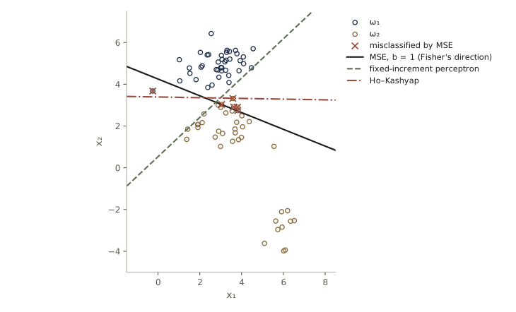
Squared error asks every sample to sit at the same value \(\mathbf{a}^{t}\mathbf{y}_i = 1\), so the far cluster of \(\omega_2\), which a separating line would classify with room to spare, pulls the MSE line toward itself and costs errors elsewhere. We draw this in the figure below, together with the other procedures.
Relation to Fisher’s linear discriminant
With the right margin vector, the MSE solution is Fisher’s linear discriminant, which we met in module 03 as the projection that best separates two classes. Order the samples so that the \(n_1\) samples of \(\omega_1\) (the set \(\mathcal{D}_1\)) come first, and write \(\mathbf{X}_i\) for the \(n_i \times d\) matrix of the unaugmented samples of class \(i\) and \(\mathbf{1}_i\) for a column of \(n_i\) ones. After normalization,
\[\mathbf{Y} = \begin{pmatrix} \mathbf{1}_1 & \mathbf{X}_1 \\ -\mathbf{1}_2 & -\mathbf{X}_2 \end{pmatrix}, \qquad \mathbf{a} = \begin{pmatrix} w_0 \\ \mathbf{w} \end{pmatrix}, \qquad \mathbf{b} = \begin{pmatrix} \beta_1\mathbf{1}_1 \\ \beta_2\mathbf{1}_2 \end{pmatrix},\]where we allow any two positive constants \(\beta_1, \beta_2\) as targets. With the sample means \(\mathbf{m}_i\), the overall mean \(\mathbf{m} = (n_1\mathbf{m}_1 + n_2\mathbf{m}_2)/n\), and the within-class scatter \(\mathbf{S}_W = \sum_i\sum_{\mathbf{x} \in \mathcal{D}_i}(\mathbf{x} - \mathbf{m}_i)(\mathbf{x} - \mathbf{m}_i)^{t}\), multiplying out the normal equations \(\mathbf{Y}^{t}\mathbf{Y}\mathbf{a} = \mathbf{Y}^{t}\mathbf{b}\) gives two equations:
\[\begin{aligned} n\,w_0 + n\,\mathbf{m}^{t}\mathbf{w} &= n_1\beta_1 - n_2\beta_2, \\ n\,\mathbf{m}\,w_0 + \left(\mathbf{S}_W + n_1\mathbf{m}_1\mathbf{m}_1^{t} + n_2\mathbf{m}_2\mathbf{m}_2^{t}\right)\mathbf{w} &= n_1\beta_1\mathbf{m}_1 - n_2\beta_2\mathbf{m}_2 . \end{aligned}\]The first gives \(w_0 = (n_1\beta_1 - n_2\beta_2)/n - \mathbf{m}^{t}\mathbf{w}\). Substituting it into the second and using two identities that follow from the definition of \(\mathbf{m}\) (exercise 5),
\[n_1\mathbf{m}_1\mathbf{m}_1^{t} + n_2\mathbf{m}_2\mathbf{m}_2^{t} - n\,\mathbf{m}\mathbf{m}^{t} = \frac{n_1n_2}{n}(\mathbf{m}_1 - \mathbf{m}_2)(\mathbf{m}_1 - \mathbf{m}_2)^{t}, \qquad n_1\beta_1(\mathbf{m}_1 - \mathbf{m}) - n_2\beta_2(\mathbf{m}_2 - \mathbf{m}) = \frac{n_1n_2}{n}(\beta_1 + \beta_2)(\mathbf{m}_1 - \mathbf{m}_2),\]we get
\[\left[\mathbf{S}_W + \frac{n_1n_2}{n}(\mathbf{m}_1 - \mathbf{m}_2)(\mathbf{m}_1 - \mathbf{m}_2)^{t}\right]\mathbf{w} = \frac{n_1n_2}{n}(\beta_1 + \beta_2)(\mathbf{m}_1 - \mathbf{m}_2).\]The rank-one term applied to \(\mathbf{w}\) points along \(\mathbf{m}_1 - \mathbf{m}_2\) whatever \(\mathbf{w}\) is, so move it to the right-hand side: \(\mathbf{S}_W\mathbf{w} = c\,(\mathbf{m}_1 - \mathbf{m}_2)\) for a scalar \(c\), which works out to be positive (exercise 5). Hence
Result. For any margin vector that is constant within each class, the MSE weight vector is \(\mathbf{w} \propto \mathbf{S}_W^{-1}(\mathbf{m}_1 - \mathbf{m}_2)\), Fisher’s direction. The margins only move the threshold. DHS’s choice \(\beta_i = n/n_i\) makes \(n_1\beta_1 = n_2\beta_2\), so \(w_0 = -\mathbf{m}^{t}\mathbf{w}\): decide \(\omega_1\) when \(\mathbf{w}^{t}(\mathbf{x} - \mathbf{m}) > 0\).
The next cell checks this on our data for three margin vectors. Our classes have equal sizes, so DHS’s choice is just \(\mathbf{b} = 2\cdot\mathbf{1}\); the third choice, \(\beta_1 = 1\) and \(\beta_2 = 3\), is deliberately lopsided.
def fisher_direction(X1, X2):
    """S_W^{-1} (m1 - m2), with S_W the (unnormalized) within-class scatter matrix."""
    m1, m2 = X1.mean(axis=0), X2.mean(axis=0)
    S_W = (X1 - m1).T @ (X1 - m1) + (X2 - m2).T @ (X2 - m2)
    return np.linalg.solve(S_W, m1 - m2)

X1s, X2s = Xs[labs == 0], Xs[labs == 1]
n1, n2, n = len(X1s), len(X2s), len(Xs)
w_fisher = fisher_direction(X1s, X2s)
m_all = Xs.mean(axis=0)
for name, beta1, beta2 in [("n/n_i", n / n1, n / n2), ("ones", 1.0, 1.0), ("(1, 3)", 1.0, 3.0)]:
    b_vec = np.where(labs == 0, beta1, beta2)
    a_b = np.linalg.lstsq(Ys, b_vec, rcond=None)[0]
    w0_b, w_b = a_b[0], a_b[1:]
    cos = w_b @ w_fisher / (np.linalg.norm(w_b) * np.linalg.norm(w_fisher))
    w0_pred = (n1 * beta1 - n2 * beta2) / n - m_all @ w_b
    print(f"b = {name:6s}: cos(w, Fisher) = {cos:.8f};  w0 = {w0_b:8.4f}, formula {w0_pred:8.4f};  "
          f"errors {np.sum(Ys @ a_b <= 0)}")

proj = np.sort(Xs @ w_fisher)                          # try every threshold on Fisher's projection
cuts = np.r_[proj[0] - 1, (proj[1:] + proj[:-1]) / 2, proj[-1] + 1]
fewest = min(np.sum((Xs @ w_fisher > t) != (labs == 0)) for t in cuts)
print(f"fewest errors of any threshold on Fisher's direction: {fewest}")
b = n/n_i : cos(w, Fisher) = 1.00000000;  w0 =  -2.8842, formula  -2.8842;  errors 6
b = ones  : cos(w, Fisher) = 1.00000000;  w0 =  -1.4421, formula  -1.4421;  errors 6
b = (1, 3): cos(w, Fisher) = 1.00000000;  w0 =  -3.8842, formula  -3.8842;  errors 11
fewest errors of any threshold on Fisher's direction: 2
The three weight vectors all point along Fisher’s direction to eight decimal places, and the threshold follows the formula. Notice the last line: no threshold on Fisher’s direction separates these data, although they are separable. Fisher’s criterion is about means and scatter, not about the samples nearest the boundary, and the far cluster distorts both the mean of \(\omega_2\) and its scatter.
Asymptotic approximation to an optimal discriminant
The second property: with \(\mathbf{b} = \mathbf{1}\), the MSE discriminant \(\mathbf{a}^{t}\mathbf{y}\) approaches, as \(n \to \infty\), the best mean-square approximation to the Bayes discriminant
\[g_0(\mathbf{x}) = P(\omega_1 \mid \mathbf{x}) - P(\omega_2 \mid \mathbf{x}) .\]Here \(\mathbf{y} = \mathbf{y}(\mathbf{x})\) can be any fixed \(\varphi\)-mapping, so \(\mathbf{a}^{t}\mathbf{y}\) is a series expansion of a discriminant. Assume the samples are drawn independently from the mixture \(p(\mathbf{x}) = p(\mathbf{x} \mid \omega_1)P(\omega_1) + p(\mathbf{x} \mid \omega_2)P(\omega_2)\). Undoing the normalization, \(\mathbf{b} = \mathbf{1}\) means target \(+1\) for \(\omega_1\) samples and \(-1\) for \(\omega_2\) samples:
\[J_s(\mathbf{a}) = \sum_{\mathbf{x} \in \mathcal{D}_1} (\mathbf{a}^{t}\mathbf{y} - 1)^2 + \sum_{\mathbf{x} \in \mathcal{D}_2} (\mathbf{a}^{t}\mathbf{y} + 1)^2 .\]By the law of large numbers, \(J_s/n\) tends with probability one to
\[\bar{J}(\mathbf{a}) = \int (\mathbf{a}^{t}\mathbf{y} - 1)^2\, p(\mathbf{x}, \omega_1)\, d\mathbf{x} + \int (\mathbf{a}^{t}\mathbf{y} + 1)^2\, p(\mathbf{x}, \omega_2)\, d\mathbf{x} .\]Expand the squares and use \(p(\mathbf{x}, \omega_1) + p(\mathbf{x}, \omega_2) = p(\mathbf{x})\) and \(p(\mathbf{x}, \omega_1) - p(\mathbf{x}, \omega_2) = g_0(\mathbf{x})p(\mathbf{x})\):
\[\begin{aligned} \bar{J}(\mathbf{a}) &= \int (\mathbf{a}^{t}\mathbf{y})^2 p(\mathbf{x})\,d\mathbf{x} - 2\int \mathbf{a}^{t}\mathbf{y}\,g_0(\mathbf{x})\,p(\mathbf{x})\,d\mathbf{x} + 1 \\ &= \underbrace{\int \left[\mathbf{a}^{t}\mathbf{y} - g_0(\mathbf{x})\right]^2 p(\mathbf{x})\,d\mathbf{x}}_{\epsilon^2(\mathbf{a})} + \underbrace{\left[1 - \int g_0^2(\mathbf{x})\,p(\mathbf{x})\,d\mathbf{x}\right]}_{\text{independent of } \mathbf{a}} . \end{aligned}\]So minimizing \(J_s\) for large \(n\) minimizes \(\epsilon^2\), the mean-squared error between \(\mathbf{a}^{t}\mathbf{y}\) and \(g_0\), weighted by \(p(\mathbf{x})\). Through \(P(\omega_1 \mid \mathbf{x}) = (1 + g_0)/2\) the MSE discriminant therefore also approximates the posterior probabilities. The catch is the weighting: the approximation is good where samples are plentiful, not necessarily near the decision boundary \(g_0 = 0\) where it matters for classification. So the MSE discriminant that best approximates the Bayes discriminant need not minimize the probability of error.
We test this in one dimension, with \(p(x \mid \omega_1) = N(1, 1)\), \(p(x \mid \omega_2) = N(-1, 0.5^2)\), equal priors, and a cubic expansion \(\mathbf{y} = (1, x, x^2, x^3)^{t}\). The limit \(\mathbf{a}^{*}\) that minimizes \(\epsilon^2\) is the solution of \(\left(\int \mathbf{y}\mathbf{y}^{t}p\,dx\right)\mathbf{a} = \int \mathbf{y}\,g_0\,p\,dx\), which we compute by numerical integration on a fine grid.
def gauss_pdf(x, mu, sigma):
    return np.exp(-0.5 * ((x - mu) / sigma) ** 2) / (sigma * np.sqrt(2 * np.pi))

def poly_features(x, degree=3):
    return np.column_stack([x ** j for j in range(degree + 1)])

xq = np.linspace(-9, 9, 36001)                               # quadrature grid
dx = xq[1] - xq[0]
pj1, pj2 = 0.5 * gauss_pdf(xq, 1.0, 1.0), 0.5 * gauss_pdf(xq, -1.0, 0.5)    # p(x, omega_i)
px = pj1 + pj2
g0 = (pj1 - pj2) / px                                        # Bayes discriminant P1 - P2
Pq = poly_features(xq)
a_star = np.linalg.solve(Pq.T @ (Pq * px[:, None]) * dx, Pq.T @ (g0 * px) * dx)

rng_b = np.random.default_rng(41)
for n_b in [200, 2000, 200000]:
    lab_b = rng_b.integers(0, 2, n_b)                        # equal priors
    x_b = np.where(lab_b == 0, rng_b.normal(1.0, 1.0, n_b), rng_b.normal(-1.0, 0.5, n_b))
    a_b = np.linalg.lstsq(normalize(poly_features(x_b), lab_b), np.ones(n_b), rcond=None)[0]
    print(f"n = {n_b:6d}: a = {a_b}   distance to a* {np.linalg.norm(a_b - a_star):.4f}")
print(f"limit a*    : {a_star}")

x_show = np.array([-1.0, 0.0, 1.0, 2.0, 4.0])
post_true = np.interp(x_show, xq, pj1 / px)
post_mse = (1 + poly_features(x_show) @ a_star) / 2
print("x               :", x_show)
print("p(x)            :", np.interp(x_show, xq, px))
print("P(omega_1 | x)  :", post_true)
print("(1 + a*^t y) / 2:", post_mse)
n =    200: a = [-0.0211  0.9548  0.0317 -0.0972]   distance to a* 0.1556
n =   2000: a = [ 0.1089  0.9202 -0.0171 -0.0739]   distance to a* 0.0618
n = 200000: a = [ 0.0947  0.8641 -0.0143 -0.0615]   distance to a* 0.0047
limit a*    : [ 0.0903  0.8628 -0.0134 -0.061 ]
x               : [-1.  0.  1.  2.  4.]
p(x)            : [0.4259 0.175  0.1996 0.121  0.0022]
P(omega_1 | x)  : [0.0634 0.6914 0.9993 1.     1.    ]
(1 + a*^t y) / 2: [0.1376 0.5452 0.9394 1.1372 0.2119]
The sample MSE solutions settle on \(\mathbf{a}^{*}\) as \(n\) grows. Where the data are dense (\(x\) from \(-1\) to \(1\)) the cubic follows the posterior to within about 0.15 — a cubic cannot match it everywhere, so it compromises — and just beyond, at \(x = 2\), it already strays above 1. At \(x = 4\), where \(p(x)\) is tiny, it reports 0.21 for a posterior that is essentially 1. The fit spends its accuracy where \(p(\mathbf{x})\) is large, exactly as the derivation predicts. The same property — least squares with 0/1 or \(\pm 1\) targets estimates posteriors — reappears for multilayer networks in module 06.
The Widrow–Hoff or LMS procedure
The criterion \(J_s\) can also be minimized by gradient descent, which avoids trouble when \(\mathbf{Y}^{t}\mathbf{Y}\) is singular and avoids large matrices. The batch rule is \(\mathbf{a}(k+1) = \mathbf{a}(k) + \eta(k)\mathbf{Y}^{t}(\mathbf{b} - \mathbf{Y}\mathbf{a}(k))\), the gradient descent we ran earlier; with \(\eta(k) = \eta(1)/k\) it converges to a solution of \(\mathbf{Y}^{t}(\mathbf{Y}\mathbf{a} - \mathbf{b}) = \mathbf{0}\) whether or not \(\mathbf{Y}^{t}\mathbf{Y}\) is singular (DHS Problem 26). Taking one sample at a time gives the Widrow–Hoff or least-mean-squares (LMS) rule:
\[\mathbf{a}(k+1) = \mathbf{a}(k) + \eta(k)\left(b_k - \mathbf{a}(k)^{t}\mathbf{y}^k\right)\mathbf{y}^k .\]It looks like single-sample relaxation, but there is a basic difference. Relaxation is an error-correcting rule: it acts only when a sample violates its margin, and on separable data the corrections can stop. LMS corrects every sample every time, because \(\mathbf{a}^{t}\mathbf{y}^k\) is almost never exactly \(b_k\); with a constant \(\eta\) it never settles, so \(\eta(k)\) must decrease. The exact analysis of the deterministic case is involved; the answer is that the sequence tends toward the MSE solution, which need not be a separating vector even when one exists. The speed depends heavily on the schedule and on the scaling of the features.
def lms(Y, b, eta, passes, checkpoints=()):
    """Widrow-Hoff rule, cycling through the samples; eta(k) with k counting single-sample steps."""
    a, k, snaps = np.zeros(Y.shape[1]), 0, []
    for p in range(1, passes + 1):
        for y, b_k in zip(Y, b):
            k += 1
            a = a + eta(k) * (b_k - a @ y) * y          # a <- a + eta(k) (b_k - a^t y^k) y^k
        if p in checkpoints:
            snaps.append(a.copy())
    return a, snaps

Zs = (Xs - Xs.mean(axis=0)) / Xs.std(axis=0)              # standardized features
Yz = normalize(augment(Zs), labs)
a_mse_z = np.linalg.lstsq(Yz, np.ones(n), rcond=None)[0]
runs = [("raw features, eta = 0.01/k", Ys, a_mse, lambda k: 0.01 / k),
        ("standardized, eta = 1/k", Yz, a_mse_z, lambda k: 1.0 / k),
        ("standardized, eta = 0.1/(1 + k/n)", Yz, a_mse_z, lambda k: 0.1 / (1 + k / n))]
print("relative distance to the MSE solution after 10, 100, 1000 passes")
for name, Y_run, target, eta in runs:
    _, snaps = lms(Y_run, np.ones(n), eta, 1000, checkpoints=(10, 100, 1000))
    rel = [np.linalg.norm(s - target) / np.linalg.norm(target) for s in snaps]
    print(f"  {name:34s}: " + ", ".join(f"{r:.1e}" for r in rel))
print(f"condition number of Y^t Y: raw {np.linalg.cond(Ys.T @ Ys):.0f}, "
      f"standardized {np.linalg.cond(Yz.T @ Yz):.1f}")
relative distance to the MSE solution after 10, 100, 1000 passes
  raw features, eta = 0.01/k        : 9.9e-01, 9.9e-01, 9.8e-01
  standardized, eta = 1/k           : 1.5e-01, 6.4e-02, 2.8e-02
  standardized, eta = 0.1/(1 + k/n) : 9.1e-03, 1.1e-03, 1.1e-04
condition number of Y^t Y: raw 464, standardized 4.5
On the raw features, whose \(\mathbf{Y}^{t}\mathbf{Y}\) is badly conditioned, a small \(1/k\) schedule barely moves in 80,000 steps. Standardizing the features fixes the conditioning; then \(1/k\) converges slowly, and a schedule that decreases once per pass rather than once per sample converges quickly. A programmed decrease that ignores the problem at hand is often painfully slow.
In practice. Before running LMS, or any of the gradient rules in this module, center and scale the features. It costs nothing, it changes none of the separability questions (an invertible affine map of \(\mathbf{x}\) preserves linear separability), and it can turn a hopeless learning-rate schedule into a fast one.
Stochastic approximation methods
So far the samples were a fixed set. Suppose instead they arrive as an endless stream of independent pairs \((\mathbf{x}_k, \theta_k)\), with \(\theta = +1\) for \(\omega_1\) and \(\theta = -1\) for \(\omega_2\). The label is a noisy version of the Bayes discriminant: \(P(\theta = 1 \mid \mathbf{x}) = P(\omega_1 \mid \mathbf{x})\), so \(\mathcal{E}[\theta \mid \mathbf{x}] = P(\omega_1 \mid \mathbf{x}) - P(\omega_2 \mid \mathbf{x}) = g_0(\mathbf{x})\). Minimizing the mean-square approximation error \(\mathcal{E}[(\mathbf{a}^{t}\mathbf{y} - g_0(\mathbf{x}))^2]\) looks as if it needs \(g_0\), but, as in the asymptotic argument, it has the same minimizer as
\[J_m(\mathbf{a}) = \mathcal{E}\left[(\mathbf{a}^{t}\mathbf{y} - \theta)^2\right], \qquad \hat{\mathbf{a}} = \mathcal{E}[\mathbf{y}\mathbf{y}^{t}]^{-1}\,\mathcal{E}[\theta\,\mathbf{y}] .\]We could estimate the two expectations and solve. Or we could descend on \(J_m\) using the noisy gradient from one sample, \(2(\mathbf{a}^{t}\mathbf{y}_k - \theta_k)\mathbf{y}_k\), which is the LMS rule again. If \(\mathcal{E}[\mathbf{y}\mathbf{y}^{t}]\) is nonsingular and
\[\sum_{k=1}^{\infty}\eta(k) = \infty, \qquad \sum_{k=1}^{\infty}\eta^2(k) < \infty,\]then \(\mathbf{a}(k)\) converges to \(\hat{\mathbf{a}}\) in mean square, \(\lim_{k\to\infty}\mathcal{E}[\lVert \mathbf{a}(k) - \hat{\mathbf{a}} \rVert^2] = 0\). The first condition keeps the steps from dying out before a systematic error is corrected; the second makes the random fluctuations die out. \(\eta(k) = 1/k\) satisfies both. Procedures of this kind — finding the minimum or the root of a regression function \(\mathcal{E}[f(\mathbf{a}, \mathbf{x})]\) from noisy evaluations — are called stochastic approximation; the Robbins–Monro procedure (root finding) and the Kiefer–Wolfowitz procedure (minimization) are the classical examples, and proofs for particular rules often reduce to theirs.
A faster rule uses second-order information. The Hessian of \(J_m\) is \(2\mathcal{E}[\mathbf{y}\mathbf{y}^{t}]\), and a stochastic version of Newton’s method replaces the scalar rate by a matrix, \(\mathbf{a}(k+1) = \mathbf{a}(k) + \mathbf{R}_{k+1}(\theta_k - \mathbf{a}(k)^{t}\mathbf{y}_k)\mathbf{y}_k\) with \(\mathbf{R}_{k+1}^{-1} = \mathbf{R}_k^{-1} + \mathbf{y}_k\mathbf{y}_k^{t}\). The inverse never needs to be formed: by the Sherman–Morrison identity,
\[\mathbf{R}_{k+1} = \mathbf{R}_k - \frac{\mathbf{R}_k\mathbf{y}_k(\mathbf{R}_k\mathbf{y}_k)^{t}}{1 + \mathbf{y}_k^{t}\mathbf{R}_k\mathbf{y}_k}.\]This is recursive least squares: after \(k\) samples, \(\mathbf{a}(k+1)\) is the least-squares solution for those samples (plus a tiny ridge term from the starting \(\mathbf{R}_1\)). It costs \(O(\hat{d}^2)\) per sample instead of \(O(\hat{d})\) and converges much faster. We compare the two on a stream from our one-dimensional problem, with the target \(\mathbf{a}^{*}\) computed above. To keep LMS stable we feed it the powers of \(x/2\) rather than \(x\) (large powers of \(x\) would force a tiny rate); in that basis the target is \(a^{*}_j 2^j\).
rng_sa = np.random.default_rng(43)
N_sa = 20000
lab_sa = rng_sa.integers(0, 2, N_sa)
x_sa = np.where(lab_sa == 0, rng_sa.normal(1.0, 1.0, N_sa), rng_sa.normal(-1.0, 0.5, N_sa))
theta_sa = np.where(lab_sa == 0, 1.0, -1.0)
Y_sa = poly_features(x_sa / 2)                                         # features of x/2: tamer scales
a_star_sa = a_star * 2.0 ** np.arange(4)                                # a* in the rescaled basis

a_lms, a_rls, R = np.zeros(4), np.zeros(4), 1e3 * np.eye(4)
for k, (y, th) in enumerate(zip(Y_sa, theta_sa), start=1):
    a_lms = a_lms + (0.1 / (1 + k / 100)) * (th - a_lms @ y) * y       # LMS, decreasing rate
    Ry = R @ y
    R = R - np.outer(Ry, Ry) / (1 + y @ Ry)                             # Sherman-Morrison update
    a_rls = a_rls + R @ y * (th - a_rls @ y)                            # stochastic Newton / RLS
    if k in (200, 2000, 20000):
        a_batch_k = np.linalg.lstsq(Y_sa[:k], theta_sa[:k], rcond=None)[0]
        print(f"k = {k:5d}: ||a - a*||  LMS {np.linalg.norm(a_lms - a_star_sa):.4f}  "
              f"RLS {np.linalg.norm(a_rls - a_star_sa):.4f}   "
              f"(||RLS - batch LS|| {np.linalg.norm(a_rls - a_batch_k):.1e})")
k =   200: ||a - a*||  LMS 0.5053  RLS 0.1898   (||RLS - batch LS|| 8.5e-05)
k =  2000: ||a - a*||  LMS 0.1017  RLS 0.0327   (||RLS - batch LS|| 1.0e-05)
k = 20000: ||a - a*||  LMS 0.0248  RLS 0.0159   (||RLS - batch LS|| 9.8e-07)
Recursive least squares tracks the least-squares solution of the samples seen so far (up to the tiny ridge term from \(\mathbf{R}_1\)), and so approaches \(\mathbf{a}^{*}\) as fast as the data allow; LMS with a scalar rate gets there too, but more slowly, because one rate has to serve features of very different scales.
The Ho–Kashyap procedures
The perceptron and relaxation rules find a separating vector when one exists but never settle otherwise. MSE always settles but may miss a separating vector that exists. Can we get the best of both? If the samples are separable, there is some \(\hat{\mathbf{a}}\) and some \(\hat{\mathbf{b}} > \mathbf{0}\) (every component positive) with \(\mathbf{Y}\hat{\mathbf{a}} = \hat{\mathbf{b}}\); MSE with that margin vector would find a separating vector. We do not know \(\hat{\mathbf{b}}\), so let us learn it: minimize
\[J_s(\mathbf{a}, \mathbf{b}) = \lVert \mathbf{Y}\mathbf{a} - \mathbf{b} \rVert^2\]over both \(\mathbf{a}\) and \(\mathbf{b}\), subject to \(\mathbf{b} > \mathbf{0}\). On separable data the minimum is zero and the minimizing \(\mathbf{a}\) separates.
The descent procedure
The gradients are \(\nabla_{\mathbf{a}}J_s = 2\mathbf{Y}^{t}(\mathbf{Y}\mathbf{a} - \mathbf{b})\) and \(\nabla_{\mathbf{b}}J_s = -2(\mathbf{Y}\mathbf{a} - \mathbf{b})\). For any \(\mathbf{b}\), the best \(\mathbf{a}\) is \(\mathbf{Y}^{\dagger}\mathbf{b}\), found in one step. For \(\mathbf{b}\) we must respect \(\mathbf{b} > \mathbf{0}\) and avoid a descent that shrinks \(\mathbf{b}\) to zero. The simple fix: start with \(\mathbf{b} > \mathbf{0}\) and never decrease any component. Following the negative gradient \(2\mathbf{e}\), but only in the components where it is positive, gives the Ho–Kashyap rule:
\[\begin{aligned} \mathbf{e}(k) &= \mathbf{Y}\mathbf{a}(k) - \mathbf{b}(k), \qquad \mathbf{e}^{+}(k) = \tfrac{1}{2}\left(\mathbf{e}(k) + \lvert \mathbf{e}(k) \rvert\right), \\ \mathbf{b}(k+1) &= \mathbf{b}(k) + 2\eta\,\mathbf{e}^{+}(k), \qquad \mathbf{a}(k+1) = \mathbf{Y}^{\dagger}\mathbf{b}(k+1), \end{aligned}\]with \(\mathbf{b}(1) > \mathbf{0}\) and \(\mathbf{a}(1) = \mathbf{Y}^{\dagger}\mathbf{b}(1)\). Here \(\lvert \mathbf{e} \rvert\) is taken component by component, so \(\mathbf{e}^{+}\), the positive part of \(\mathbf{e}\), keeps the positive components of \(\mathbf{e}\) and zeros the rest: a component of \(\mathbf{b}\) grows when the sample already exceeds its target, \(\mathbf{a}^{t}\mathbf{y}_i > b_i\), which is harmless, and is left alone otherwise. Because \(\mathbf{a}\) is determined by \(\mathbf{b}\), this is really an iteration on margin vectors. It stops changing only when \(\mathbf{e}^{+} = \mathbf{0}\), and then there are two possibilities: \(\mathbf{e} = \mathbf{0}\), and we have a solution; or \(\mathbf{e} \le \mathbf{0}\) with some component negative, which, we will show, proves that no separating vector exists.
Convergence proof
Two facts about \(\mathbf{Y}\mathbf{Y}^{\dagger}\) do the work (we assume \(\mathbf{Y}^{t}\mathbf{Y}\) nonsingular for simplicity; the results hold in general). Since \(\mathbf{Y}\mathbf{Y}^{\dagger} = \mathbf{Y}(\mathbf{Y}^{t}\mathbf{Y})^{-1}\mathbf{Y}^{t}\), it is symmetric, positive semidefinite, and idempotent, \((\mathbf{Y}\mathbf{Y}^{\dagger})^2 = \mathbf{Y}\mathbf{Y}^{\dagger}\): it is the orthogonal projection onto the column space of \(\mathbf{Y}\). And because \(\mathbf{a}(k)\) solves the normal equations for \(\mathbf{b}(k)\), the error is orthogonal to that column space: \(\mathbf{Y}^{t}\mathbf{e}(k) = \mathbf{0}\).
Step 1: on separable data, \(\mathbf{e}^{+}(k) = \mathbf{0}\) only if \(\mathbf{e}(k) = \mathbf{0}\). Separability gives \(\hat{\mathbf{a}}\) with \(\mathbf{Y}\hat{\mathbf{a}} = \hat{\mathbf{b}} > \mathbf{0}\). Then \(\mathbf{e}(k)^{t}\hat{\mathbf{b}} = \mathbf{e}(k)^{t}\mathbf{Y}\hat{\mathbf{a}} = \mathbf{0}^{t}\hat{\mathbf{a}} = 0\). A nonzero vector with no positive component has a negative inner product with a positive vector, so a nonzero \(\mathbf{e}(k)\) must have some positive component.
Step 2: \(\lVert \mathbf{e}(k) \rVert^2\) decreases. Eliminating \(\mathbf{a}\), \(\mathbf{e}(k) = (\mathbf{Y}\mathbf{Y}^{\dagger} - \mathbf{I})\mathbf{b}(k)\), so
\[\mathbf{e}(k+1) = (\mathbf{Y}\mathbf{Y}^{\dagger} - \mathbf{I})\left(\mathbf{b}(k) + 2\eta\,\mathbf{e}^{+}(k)\right) = \mathbf{e}(k) + 2\eta(\mathbf{Y}\mathbf{Y}^{\dagger} - \mathbf{I})\mathbf{e}^{+}(k).\]Expand \(\lVert \mathbf{e}(k+1) \rVert^2\). The cross term is \(4\eta\,\mathbf{e}^{t}(\mathbf{Y}\mathbf{Y}^{\dagger} - \mathbf{I})\mathbf{e}^{+} = -4\eta\,\mathbf{e}^{t}\mathbf{e}^{+} = -4\eta\lVert \mathbf{e}^{+} \rVert^2\), because \(\mathbf{e}^{t}\mathbf{Y} = \mathbf{0}^{t}\) and the positive components of \(\mathbf{e}\) are exactly those of \(\mathbf{e}^{+}\). The square term is \(4\eta^2\,\mathbf{e}^{+t}(\mathbf{I} - \mathbf{Y}\mathbf{Y}^{\dagger})\mathbf{e}^{+}\), since \(\mathbf{I} - \mathbf{Y}\mathbf{Y}^{\dagger}\) is also a symmetric projection. Altogether (dropping the argument \(k\)),
\[\frac{1}{4}\left(\lVert \mathbf{e}(k) \rVert^2 - \lVert \mathbf{e}(k+1) \rVert^2\right) = \eta(1 - \eta)\lVert \mathbf{e}^{+} \rVert^2 + \eta^2\,\mathbf{e}^{+t}\mathbf{Y}\mathbf{Y}^{\dagger}\mathbf{e}^{+}.\]With \(0 < \eta < 1\) both terms are nonnegative and the first is positive whenever \(\mathbf{e}^{+} \ne \mathbf{0}\).
Step 3: the error goes to zero. The decreasing sequence \(\lVert \mathbf{e}(k) \rVert^2\) converges, so the decrements, and with them \(\lVert \mathbf{e}^{+}(k) \rVert\), go to zero. Write \(\mathbf{e} = \mathbf{e}^{+} - \mathbf{e}^{-}\) with \(\mathbf{e}^{-} \ge \mathbf{0}\). From Step 1, \(\mathbf{e}^{-t}\hat{\mathbf{b}} = \mathbf{e}^{+t}\hat{\mathbf{b}} \to 0\), and since every component of \(\hat{\mathbf{b}}\) is positive, \(\mathbf{e}^{-} \to \mathbf{0}\) too. So \(\mathbf{e}(k) \to \mathbf{0}\).
Step 4: a separating vector appears after finitely many steps. \(\mathbf{Y}\mathbf{a}(k) = \mathbf{b}(k) + \mathbf{e}(k)\), and the components of \(\mathbf{b}(k)\) never decrease, so they stay at least \(b_{\min}\), the smallest component of \(\mathbf{b}(1)\). Once \(\lVert \mathbf{e}(k) \rVert < b_{\min}\), every component of \(\mathbf{Y}\mathbf{a}(k)\) is positive. \(\square\)
Result (Ho–Kashyap). With \(0 < \eta < 1\), the Ho–Kashyap rule on linearly separable samples reaches a separating vector in finitely many steps (checking the signs of \(\mathbf{Y}\mathbf{a}(k)\) at each step). If at some step \(\mathbf{e}(k) \le \mathbf{0}\) with \(\mathbf{e}(k) \ne \mathbf{0}\), the samples are not linearly separable.
def ho_kashyap(Y, eta=0.5, b=None, k_max=20000, tol=1e-9):
    """Ho-Kashyap rule. Returns (a, b, steps, verdict, history of (||e||^2, ||e+||^2))."""
    Y_pinv = np.linalg.pinv(Y)
    b = np.ones(len(Y)) if b is None else np.array(b, float)
    a = Y_pinv @ b
    hist = []
    for k in range(1, k_max + 1):
        e = Y @ a - b
        e_plus = 0.5 * (e + np.abs(e))
        hist.append((e @ e, e_plus @ e_plus))
        if np.all(Y @ a > 0):
            return a, b, k, "separating vector", np.array(hist)
        if e_plus.max() < tol:                        # e <= 0 but e != 0: proof of nonseparability
            return a, b, k, "not separable (e <= 0)", np.array(hist)
        b = b + 2 * eta * e_plus                      # b(k+1) = b(k) + 2 eta e+(k)
        a = Y_pinv @ b                                # a(k+1) = Y+ b(k+1)
    return a, b, k_max, "undecided", np.array(hist)

a_hk, b_hk, k_hk, verdict, hist_hk = ho_kashyap(Ys)
print(f"separable data   : {verdict} at step {k_hk};  misclassified {np.sum(Ys @ a_hk <= 0)}")

Y_pinv_s = np.linalg.pinv(Ys)                          # check the decrease identity at one step
b_k = b_hk.copy()
e_k = Ys @ Y_pinv_s @ b_k - b_k
ep_k = np.maximum(e_k, 0)
e_next = Ys @ Y_pinv_s @ (b_k + 2 * 0.5 * ep_k) - (b_k + 2 * 0.5 * ep_k)
lhs = (e_k @ e_k - e_next @ e_next) / 4
rhs = 0.5 * 0.5 * ep_k @ ep_k + 0.25 * ep_k @ Ys @ Y_pinv_s @ ep_k
print(f"decrease identity: lhs {lhs:.6f}, rhs {rhs:.6f}")
separable data   : separating vector at step 5;  misclassified 0
decrease identity: lhs 0.364327, rhs 0.364327
On the separable data Ho–Kashyap reaches a separating vector, which MSE with a fixed \(\mathbf{b} = \mathbf{1}\) did not, by raising the margins of the samples that were already beyond their targets (above all the far cluster) until the least-squares fit no longer needs to compromise. The last line checks the decrease identity from Step 2 numerically.
Nonseparable behavior
Separability was used twice in the proof: in Step 1, to rule out a nonzero error with no positive component, and in Step 3, to conclude that \(\mathbf{e} \to \mathbf{0}\) from \(\mathbf{e}^{+} \to \mathbf{0}\). Without it, both conclusions can fail, and that is useful. If the rule ever reaches \(\mathbf{e}(k) \le \mathbf{0}\), \(\mathbf{e}(k) \ne \mathbf{0}\), Step 1 run backward proves nonseparability: if a separating \(\hat{\mathbf{a}}\) existed we would have \(\mathbf{e}^{t}\hat{\mathbf{b}} = 0\), impossible for such an \(\mathbf{e}\). If that never happens, the decrease identity still holds, so \(\lVert \mathbf{e}(k) \rVert^2\) still converges, now to a positive limit, and \(\mathbf{e}^{+}(k) \to \mathbf{0}\) while \(\mathbf{e}(k)\) stays away from zero — again evidence of nonseparability, though with no bound on how long it takes to become clear.
xor_X = np.array([[1.0, 1.0], [-1.0, -1.0], [1.0, -1.0], [-1.0, 1.0]])
xor_lab = np.array([0, 0, 1, 1])
for name, Y_test in [("XOR", normalize(augment(xor_X), xor_lab)), ("Gaussians", Yn)]:
    a_t, b_t, k_t, verdict_t, hist_t = ho_kashyap(Y_test)
    e_t = Y_test @ a_t - b_t
    print(f"{name:9s}: {verdict_t} at step {k_t:2d};  ||e||^2 = {hist_t[-1, 0]:.4f}, "
          f"max e_i = {e_t.max():.1e}")
_, _, _, _, hist_ns = ho_kashyap(Yn)
print("on the Gaussians, ||e||^2 at steps 1, 10, 30:", hist_ns[[0, 9, 29], 0])
print("                 ||e+||^2 at steps 1, 10, 30:", hist_ns[[0, 9, 29], 1])
XOR      : not separable (e <= 0) at step  1;  ||e||^2 = 4.0000, max e_i = -1.0e+00
Gaussians: not separable (e <= 0) at step 94;  ||e||^2 = 47.1399, max e_i = 8.4e-10
on the Gaussians, ||e||^2 at steps 1, 10, 30: [51.0618 47.1718 47.1399]
                 ||e+||^2 at steps 1, 10, 30: [1.3871 0.0062 0.    ]
For XOR the very first error vector is \(-\mathbf{b}\): the least-squares fit gives \(\mathbf{a} = \mathbf{0}\), and the rule stops at once with a proof. On the overlapping Gaussians the positive part of the error collapses (from about 1.4 to 0.006 in ten steps) while \(\lVert \mathbf{e} \rVert^2\) levels off near 47. At step 94 its largest component is below our tolerance of \(10^{-9}\) and the procedure declares the data nonseparable. In exact arithmetic \(\mathbf{e}^{+}\) might only tend to zero without reaching it, so in practice the test needs a tolerance.
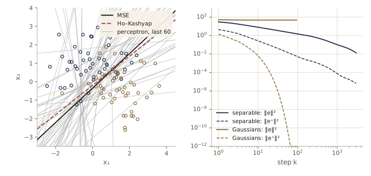
Some related procedures
Because \(\mathbf{Y}^{\dagger}\mathbf{e}(k) = \mathbf{0}\), the rule can be rewritten to update \(\mathbf{a}\) directly, \(\mathbf{b}(k+1) = \mathbf{b}(k) + \eta(\mathbf{e}(k) + \lvert \mathbf{e}(k) \rvert)\) and \(\mathbf{a}(k+1) = \mathbf{a}(k) + \eta\mathbf{Y}^{\dagger}\lvert \mathbf{e}(k) \rvert\) (the same iteration, since \(\mathbf{e} + \lvert \mathbf{e} \rvert = 2\mathbf{e}^{+}\)). Compared with the perceptron and relaxation, Ho–Kashyap varies both \(\mathbf{a}\) and \(\mathbf{b}\) and gives evidence of nonseparability, but it needs the pseudoinverse — computed once, but expensive for large \(\hat{d}\) and delicate when \(\mathbf{Y}^{t}\mathbf{Y}\) is singular.
A variant avoids the pseudoinverse altogether. Replace \(\mathbf{Y}^{\dagger}\) by \(\mathbf{R}\mathbf{Y}^{t}\) for a fixed symmetric positive definite \(\mathbf{R}\):
\[\mathbf{b}(k+1) = \mathbf{b}(k) + \left(\mathbf{e}(k) + \lvert \mathbf{e}(k) \rvert\right), \qquad \mathbf{a}(k+1) = \mathbf{a}(k) + \eta\,\mathbf{R}\mathbf{Y}^{t}\lvert \mathbf{e}(k) \rvert .\]Substituting, \(\mathbf{e}(k+1) = (\eta\mathbf{Y}\mathbf{R}\mathbf{Y}^{t} - \mathbf{I})\lvert \mathbf{e}(k) \rvert\), and a short computation gives
\[\lVert \mathbf{e}(k) \rVert^2 - \lVert \mathbf{e}(k+1) \rVert^2 = \left(\mathbf{Y}^{t}\lvert \mathbf{e}(k) \rvert\right)^{t}\left(2\eta\mathbf{R} - \eta^2\mathbf{R}\mathbf{Y}^{t}\mathbf{Y}\mathbf{R}\right)\left(\mathbf{Y}^{t}\lvert \mathbf{e}(k) \rvert\right).\]For small enough \(\eta\) the middle matrix is positive definite (for \(\mathbf{R} = \mathbf{I}\), any \(0 < \eta < 2/\lambda_{\max}\) with \(\lambda_{\max}\) the largest eigenvalue of \(\mathbf{Y}^{t}\mathbf{Y}\), which is at most \(\sum_i \lVert \mathbf{y}_i \rVert^2\)). The same argument as before then shows: on separable data a solution appears after finitely many steps; otherwise \(\mathbf{Y}^{t}\lvert \mathbf{e}(k) \rvert\) either becomes zero, proving nonseparability, or tends to zero. Choosing \(\eta\) at each step to maximize the decrease gives, for \(\mathbf{R} = \mathbf{I}\),
\[\eta(k) = \frac{\lVert \mathbf{Y}^{t}\lvert \mathbf{e}(k) \rvert \rVert^2}{\lVert \mathbf{Y}\mathbf{Y}^{t}\lvert \mathbf{e}(k) \rvert \rVert^2},\]and optimizing over \(\mathbf{R}\) as well leads back to \(\mathbf{R} \propto (\mathbf{Y}^{t}\mathbf{Y})^{-1}\), the original procedure.
def ho_kashyap_R_identity(Y, k_max=20000, tol=1e-9):
    """The pseudoinverse-free variant with R = I and the optimal eta(k)."""
    a, b = np.zeros(Y.shape[1]), np.ones(len(Y))
    for k in range(1, k_max + 1):
        if np.all(Y @ a > 0):
            return a, k, "separating vector found"
        e = Y @ a - b
        g = Y.T @ np.abs(e)                          # Y^t |e|
        if np.linalg.norm(g) < tol:
            return a, k, "not linearly separable (Y^t |e| = 0)"
        eta = (g @ g) / np.sum((Y @ g) ** 2)          # optimal step for R = I
        b = b + (e + np.abs(e))
        a = a + eta * g
    return a, k_max, "undecided"

for name, Y_test in [("separable data", Ys), ("overlapping Gaussians", Yn)]:
    a_v, k_v, verdict_v = ho_kashyap_R_identity(Y_test)
    print(f"{name:22s}: {verdict_v} after {k_v} steps")
separable data        : separating vector found after 51 steps
overlapping Gaussians : not linearly separable (Y^t |e| = 0) after 41 steps
Linear programming algorithms
Everything so far — perceptron, relaxation, Ho–Kashyap — has been a descent method for linear inequalities. Linear programming is the classical machinery for optimizing a linear function subject to linear inequality constraints, so it is natural to hand our inequalities to it. (This section is starred in DHS: specialized, but short.)
Linear programming
A standard linear program asks for a vector \(\mathbf{u} = (u_1, \dots, u_m)^{t}\) that minimizes a linear objective function \(z = \boldsymbol{\alpha}^{t}\mathbf{u}\) subject to \(\mathbf{A}\mathbf{u} \ge \boldsymbol{\beta}\) and \(\mathbf{u} \ge \mathbf{0}\), where \(\boldsymbol{\alpha}\) is an \(m\)-vector of costs, \(\mathbf{A}\) an \(l \times m\) matrix, and \(\boldsymbol{\beta}\) an \(l\)-vector. The simplex algorithm solves such problems in finitely many steps by moving between vertices of the feasible region. The constraint \(\mathbf{u} \ge \mathbf{0}\) does not suit a weight vector, whose components can have either sign, so we write \(\mathbf{a} = \mathbf{a}^{+} - \mathbf{a}^{-}\) with \(\mathbf{a}^{+} = \frac{1}{2}(\lvert \mathbf{a} \rvert + \mathbf{a}) \ge \mathbf{0}\) and \(\mathbf{a}^{-} = \frac{1}{2}(\lvert \mathbf{a} \rvert - \mathbf{a}) \ge \mathbf{0}\), and put both parts into \(\mathbf{u}\).
We do not write a simplex code here. Following the guide for these notes, this is the one place we use a generic solver: scipy.optimize.linprog, whose default method (HiGHS) solves the same problems. It minimizes \(\mathbf{c}^{t}\mathbf{u}\) subject to \(\mathbf{A}_{\mathrm{ub}}\mathbf{u} \le \mathbf{b}_{\mathrm{ub}}\), so each constraint \(\mathbf{A}\mathbf{u} \ge \boldsymbol{\beta}\) goes in with its signs flipped.
The linearly separable case
We want \(\mathbf{a}\) with \(\mathbf{a}^{t}\mathbf{y}_i \ge b_i > 0\) for all \(i\). Introduce an artificial variable \(\tau \ge 0\) and relax the constraints to \(\mathbf{a}^{t}\mathbf{y}_i + \tau \ge b_i\). These are easy to satisfy — \(\mathbf{a} = \mathbf{0}\) with \(\tau = \max_i b_i\) works, which conveniently gives the simplex method a starting point — so minimize \(\tau\). If the minimum is zero, the optimal \(\mathbf{a}\) satisfies the original constraints and the samples are separable. If it is positive, no separating vector exists, and the solver has proved it. In the standard form, \(\mathbf{u} = (\mathbf{a}^{+}, \mathbf{a}^{-}, \tau)\) has \(2\hat{d} + 1\) components, the rows of \(\mathbf{A}\) are \((\mathbf{y}_i^{t}, -\mathbf{y}_i^{t}, 1)\), \(\boldsymbol{\beta} = \mathbf{b}\), and the cost vector picks out \(\tau\).
def lp_min_tau(Y, b=None):
    """Minimize tau subject to a^t y_i + tau >= b_i, with u = (a+, a-, tau) >= 0. Returns (a, tau)."""
    n, dh = Y.shape
    b = np.ones(n) if b is None else b
    A = np.column_stack([Y, -Y, np.ones(n)])                  # rows (y_i^t, -y_i^t, 1)
    cost = np.r_[np.zeros(2 * dh), 1.0]
    res = linprog(cost, A_ub=-A, b_ub=-b, bounds=[(0, None)] * (2 * dh + 1))
    return res.x[:dh] - res.x[dh:2 * dh], res.x[-1]

for name, Y_test in [("separable", Ys), ("Gaussians", Yn), ("XOR", normalize(augment(xor_X), xor_lab))]:
    a_lp, tau = lp_min_tau(Y_test)
    print(f"{name:9s}: min tau = {tau:.4f},  ||a|| = {np.linalg.norm(a_lp):7.3f},  "
          f"misclassified {np.sum(Y_test @ a_lp <= 0)}")
separable: min tau = 0.0000,  ||a|| =  11.737,  misclassified 0
Gaussians: min tau = 1.0000,  ||a|| =   0.000,  misclassified 100
XOR      : min tau = 1.0000,  ||a|| =   0.000,  misclassified 4
On separable data the optimal \(\tau\) is zero and the solution separates. On the other two sets \(\tau = 1\), a certificate of nonseparability, and the accompanying \(\mathbf{a}\) is the useless zero vector. That is no accident: with \(\mathbf{b} = \mathbf{1}\), any \(\tau < 1\) would give \(\mathbf{a}^{t}\mathbf{y}_i \ge 1 - \tau > 0\) for every sample, a separating vector; so on nonseparable data the optimum is exactly 1, and \(\mathbf{a} = \mathbf{0}\) attains it. This formulation answers the yes-or-no question and nothing more.
This gives us a way to test the claim from the nonseparable section, that a small sample is likely to be separable by chance. For \(n\) points in general position in \(d\) dimensions, T. M. Cover’s function-counting theorem says that of the \(2^n\) ways to label them, exactly \(2\sum_{i=0}^{d}\binom{n-1}{i}\) are linearly separable (with a bias, that is, with \(\hat{d} = d + 1\) weights). For \(n \le \hat{d}\) every labeling is separable, and at \(n = 2\hat{d}\) exactly half are. We label random points at random and let the linear program decide.
def cover_fraction(n_pts, d_hat):
    """Fraction of the 2^n labelings of n points in general position that are linearly separable."""
    return 2 * sum(comb(n_pts - 1, i) for i in range(d_hat)) / 2 ** n_pts

rng_cov = np.random.default_rng(77)
for n_pts in [3, 4, 6, 8, 10]:
    trials, separable = 250, 0
    for _ in range(trials):
        X_r = rng_cov.normal(size=(n_pts, 2))
        lab_r = rng_cov.integers(0, 2, n_pts)
        separable += lp_min_tau(normalize(augment(X_r), lab_r))[1] < 0.5     # tau is 0 or 1
    frac = separable / trials
    print(f"n = {n_pts:2d}: separable fraction {frac:.3f} (+/- {np.sqrt(frac * (1 - frac) / trials):.3f}),"
          f"  Cover's formula {cover_fraction(n_pts, 3):.3f}")
n =  3: separable fraction 1.000 (+/- 0.000),  Cover's formula 1.000
n =  4: separable fraction 0.880 (+/- 0.021),  Cover's formula 0.875
n =  6: separable fraction 0.476 (+/- 0.032),  Cover's formula 0.500
n =  8: separable fraction 0.184 (+/- 0.025),  Cover's formula 0.227
n = 10: separable fraction 0.068 (+/- 0.016),  Cover's formula 0.090
The simulated fractions agree with the formula to within about two standard errors (shown in parentheses). (Since the optimal \(\tau\) is either 0 or 1, testing \(\tau < 1/2\) is safe even when a separable labeling needs a very long \(\mathbf{a}\) and the solver’s answer is slightly off zero.) With \(n = 2\hat{d} = 6\) random points, a random labeling is as likely separable as not; by \(n = 10\) it rarely is. So when \(n\) is not several times \(\hat{d}\), finding a separating vector tells us very little about how the classifier will do on new data — a point module 09 develops.
Watch out. “The training data are linearly separable” is a statement about the data set, not about the problem. With \(\varphi\)-functions it gets easier and easier to satisfy — a quadratic expansion in 10 features already has 66 weights — so zero training errors from a perceptron or a linear program should be read against Cover’s count, not as evidence that the classes are separable in general.
Minimizing the perceptron criterion function
In most applications we cannot assume separability, and we would like the weight vector that classifies as many samples as possible correctly. The number of errors is not linear in \(\mathbf{a}\), so minimizing it is not a linear program. But the perceptron criterion with a margin vector,
\[J_p'(\mathbf{a}) = \sum_{\mathbf{y}_i \in \mathcal{Y}(\mathbf{a})} (b_i - \mathbf{a}^{t}\mathbf{y}_i), \qquad \mathcal{Y}(\mathbf{a}) = \{\mathbf{y}_i : \mathbf{a}^{t}\mathbf{y}_i \le b_i\},\]can be minimized exactly by linear programming. (The margin keeps the trivial minimizer \(\mathbf{a} = \mathbf{0}\) out, as we saw in the nonseparable section.) \(J_p'\) is piecewise linear, not linear, but introduce one artificial variable per sample and minimize
\[z = \sum_{i=1}^{n}\tau_i \qquad \text{subject to } \tau_i \ge 0, \quad \tau_i \ge b_i - \mathbf{a}^{t}\mathbf{y}_i .\]For fixed \(\mathbf{a}\) the best choice is \(\tau_i = \max(0, b_i - \mathbf{a}^{t}\mathbf{y}_i)\), which makes \(z = J_p'(\mathbf{a})\); minimizing over \(\mathbf{a}\) and \(\boldsymbol{\tau}\) together therefore minimizes \(J_p'\). Now \(\mathbf{u} = (\mathbf{a}^{+}, \mathbf{a}^{-}, \boldsymbol{\tau})\) has \(2\hat{d} + n\) components and there are \(n\) constraints; \(\mathbf{a} = \mathbf{0}\), \(\tau_i = b_i\) is a feasible start. On separable data the minimum is zero and gives a separating vector; on nonseparable data we get the global minimum of the criterion, something none of the descent rules could promise.
def lp_perceptron_criterion(Y, b=None):
    """Minimize sum_i tau_i subject to tau_i >= 0 and a^t y_i + tau_i >= b_i. Returns (a, optimal value)."""
    n, dh = Y.shape
    b = np.ones(n) if b is None else b
    A = np.column_stack([Y, -Y, np.eye(n)])                   # rows (y_i^t, -y_i^t, e_i^t)
    cost = np.r_[np.zeros(2 * dh), np.ones(n)]
    res = linprog(cost, A_ub=-A, b_ub=-b, bounds=[(0, None)] * (2 * dh + n))
    return res.x[:dh] - res.x[dh:2 * dh], res.fun

def J_p_margin(a, Y, b=1.0):
    return np.sum(np.maximum(b - Y @ a, 0.0))

a_jp, z_opt = lp_perceptron_criterion(Yn)
print(f"LP optimum {z_opt:.4f};  J_p'(a) recomputed {J_p_margin(a_jp, Yn):.4f};  "
      f"errors {np.sum(Yn @ a_jp <= 0)}")
for name, eta in [("1", lambda k: 1.0), ("1/k", lambda k: 1.0 / k), ("1/sqrt(k)", lambda k: k ** -0.5)]:
    a_v, _, _ = variable_increment(Yn, 1.0, eta, max_passes=300)
    print(f"variable increment, b = 1, eta(k) = {name:9s}: J_p' = {J_p_margin(a_v, Yn):7.4f}, "
          f"errors {np.sum(Yn @ a_v <= 0)}")
LP optimum 40.1468;  J_p'(a) recomputed 40.1468;  errors 18
variable increment, b = 1, eta(k) = 1        : J_p' = 198.7463, errors 38
variable increment, b = 1, eta(k) = 1/k      : J_p' = 40.6386, errors 20
variable increment, b = 1, eta(k) = 1/sqrt(k): J_p' = 40.5320, errors 18
The linear program attains a smaller \(J_p'\) than any of the descent runs, as it must, and its classifier is as good as the best of them. Linear programming guarantees convergence whether or not the data are separable, and general-purpose solvers are easy to use; its drawbacks are the cost on large problems and that, unlike the descent rules, it does not carry over to the multilayer networks of module 06. No procedure in this chapter dominates all the others; the summary table at the end of the module collects their properties.
Support vector machines
A support vector machine (SVM) combines three ideas we have already met: a \(\varphi\)-mapping to a high-dimensional space where the classes become separable, the linear discriminant in that space, and the margin — here pushed to its logical end, the separating hyperplane with the largest possible margin. (Also a starred section in DHS; Intro to ML, module 07 treats it at greater length, including the soft margin and the connection to other sparse kernel machines.)
Map each pattern \(\mathbf{x}_k\) to \(\mathbf{y}_k = \varphi(\mathbf{x}_k)\) and let \(z_k = +1\) if pattern \(k\) is in \(\omega_1\) and \(z_k = -1\) if it is in \(\omega_2\). With a mapping to a sufficiently high dimension, two sets of distinct points can always be separated by a hyperplane. We write the discriminant as
\[g(\mathbf{x}) = \mathbf{w}^{t}\mathbf{y} + w_0, \qquad \mathbf{y} = \varphi(\mathbf{x}),\]keeping the bias \(w_0\) separate from the weights. (DHS augments \(\mathbf{y}\) and puts the bias inside the weight vector; keeping it apart, unpenalized, is the more common convention and is what produces the equality constraint in the dual below.) A separating hyperplane satisfies \(z_k g(\mathbf{x}_k) > 0\) for all \(k\).
The optimal hyperplane and the support vectors
The distance from \(\mathbf{y}_k\) to the hyperplane is \(z_k g(\mathbf{x}_k)/\lVert \mathbf{w} \rVert\). We want the hyperplane that maximizes the smallest of these distances, the margin. Since \((\mathbf{w}, w_0)\) can be rescaled freely, fix the scale by requiring \(z_k g(\mathbf{x}_k) \ge 1\) for all \(k\), with equality for the closest patterns; the margin is then \(1/\lVert \mathbf{w} \rVert\), and maximizing it means
\[\text{minimize } \frac{1}{2}\lVert \mathbf{w} \rVert^2 \quad \text{subject to} \quad z_k(\mathbf{w}^{t}\mathbf{y}_k + w_0) \ge 1, \quad k = 1, \dots, n .\]The support vectors are the transformed patterns for which the constraint holds with equality: the patterns closest to the hyperplane, at distance exactly \(1/\lVert \mathbf{w} \rVert\) on either side. They are the hardest patterns to classify and, informally, the most informative ones: the optimal hyperplane depends on them alone, and removing any other pattern leaves it unchanged.
That last fact gives a neat bound on the error. Train on \(n - 1\) of the patterns and test on the one left out, and do this for each pattern in turn (the leave-one-out estimate of module 09). A pattern that is not a support vector of the full solution is classified correctly when left out, because the hyperplane does not move. So the leave-one-out error count is at most the number of support vectors \(N_s\), and taking expectations over training sets,
\[\mathcal{E}_n[P(\text{error})] \le \frac{\mathcal{E}_n[N_s]}{n},\]where, strictly, the left side refers to machines trained on \(n - 1\) patterns. The bound does not depend on the dimension of the \(\varphi\)-space at all. A mapping that separates the classes with few support vectors should generalize well, however many dimensions it uses; this is how the SVM sidesteps the curse of dimensionality that made generalized discriminants look hopeless.
The simplest training idea is a perceptron that, instead of correcting with any misclassified pattern, always corrects with the currently worst-classified one; near the end of training that pattern is a support vector. It needs a search through all patterns at every step, so it only suits small problems. The standard route goes through the dual problem.
SVM training
Attach a Lagrange multiplier \(\alpha_k \ge 0\) to each constraint and form
\[L(\mathbf{w}, w_0, \boldsymbol{\alpha}) = \frac{1}{2}\lVert \mathbf{w} \rVert^2 - \sum_{k=1}^{n}\alpha_k\left[z_k(\mathbf{w}^{t}\mathbf{y}_k + w_0) - 1\right],\]to be minimized over \(\mathbf{w}\) and \(w_0\) and maximized over \(\boldsymbol{\alpha} \ge \mathbf{0}\). Setting the derivatives with respect to \(\mathbf{w}\) and \(w_0\) to zero gives
\[\mathbf{w} = \sum_{k=1}^{n}\alpha_k z_k\mathbf{y}_k, \qquad \sum_{k=1}^{n}\alpha_k z_k = 0 .\]Substituting back, the \(w_0\) term vanishes, the first two terms combine to \(-\frac{1}{2}\lVert \mathbf{w} \rVert^2\), and what remains is the dual problem:
\[\text{maximize } L(\boldsymbol{\alpha}) = \sum_{k=1}^{n}\alpha_k - \frac{1}{2}\sum_{k=1}^{n}\sum_{j=1}^{n}\alpha_k\alpha_j z_k z_j\,\mathbf{y}_j^{t}\mathbf{y}_k \quad \text{subject to} \quad \sum_{k=1}^{n} z_k\alpha_k = 0, \quad \alpha_k \ge 0 .\]For this convex problem the Kuhn–Tucker conditions guarantee that the maximum of the dual equals the minimum of the primal, and they add complementary slackness: \(\alpha_k\left[z_k g(\mathbf{x}_k) - 1\right] = 0\) for every \(k\). So \(\alpha_k > 0\) only for support vectors, and \(\mathbf{w}\) is a combination of the support vectors alone. The bias follows from any support vector, where \(z_k g(\mathbf{x}_k) = 1\).
The patterns enter the dual only through inner products \(\mathbf{y}_j^{t}\mathbf{y}_k = \varphi(\mathbf{x}_j)^{t}\varphi(\mathbf{x}_k)\), and so does the discriminant, \(g(\mathbf{x}) = \sum_k \alpha_k z_k\,\varphi(\mathbf{x}_k)^{t}\varphi(\mathbf{x}) + w_0\). For many useful mappings this inner product is a simple kernel function \(K(\mathbf{x}_j, \mathbf{x}_k)\) of the original patterns. For the quadratic mapping \(\varphi(\mathbf{x}) = (1, \sqrt{2}x_1, \sqrt{2}x_2, \sqrt{2}x_1x_2, x_1^2, x_2^2)^{t}\) — the full quadratic expansion, with \(\sqrt{2}\) factors chosen for this purpose — expanding the square shows
\[\varphi(\mathbf{x})^{t}\varphi(\mathbf{x}') = (1 + \mathbf{x}^{t}\mathbf{x}')^2 ,\]the polynomial kernel of degree 2. We never need the \(\varphi\)-vectors themselves.
The dual is a quadratic program, and generic solvers can handle it, but a simple special-purpose method works well: sequential minimal optimization (SMO). Because of the equality constraint we cannot change one \(\alpha_k\) alone, but we can change two at once: add \(z_i t\) to \(\alpha_i\) and subtract \(z_j t\) from \(\alpha_j\), which leaves \(\sum_k z_k\alpha_k\) unchanged. The dual objective along this line is a one-dimensional quadratic in \(t\), maximized in closed form and then clipped to keep both multipliers nonnegative. For the pair, we take the one that most violates the optimality conditions. Writing \(G_k\) for the gradient of the negated dual, \(G_k = z_k\sum_j \alpha_j z_j K_{kj} - 1\), the conditions say that \(-z_kG_k\) must take the same value (which is \(w_0\)) at every pattern with \(\alpha_k > 0\), and that it must be on the correct side of \(w_0\) at the others. So we pick \(i\) with the largest \(-z_iG_i\) among patterns whose \(\alpha\) may move in the \(+z_i\) direction and \(j\) with the smallest \(-z_jG_j\) among those whose \(\alpha\) may move in the \(-z_j\) direction, and stop when the gap between the two is below a tolerance. Each step costs \(O(n)\).
def poly_kernel(X1, X2, degree=2):
    """K(x, x') = (1 + x^t x')^degree."""
    return (1.0 + X1 @ X2.T) ** degree

def smo(K, z, C=np.inf, tol=1e-9, max_iter=100000):
    """Maximize sum(alpha) - 1/2 sum_kj alpha_k alpha_j z_k z_j K_kj
    subject to sum_k z_k alpha_k = 0 and 0 <= alpha_k <= C (C = inf: hard margin).
    Sequential minimal optimization with the maximal-violating-pair rule. Returns (alpha, w0, iterations)."""
    n = len(z)
    alpha = np.zeros(n)
    Q = np.outer(z, z) * K
    G = -np.ones(n)                                     # gradient of 1/2 alpha^t Q alpha - sum(alpha)
    for it in range(1, max_iter + 1):
        score = -z * G
        up = ((z > 0) & (alpha < C)) | ((z < 0) & (alpha > 0))     # alpha_i may move by +z_i t
        low = ((z < 0) & (alpha < C)) | ((z > 0) & (alpha > 0))    # alpha_j may move by -z_j t
        i = np.flatnonzero(up)[np.argmax(score[up])]
        j = np.flatnonzero(low)[np.argmin(score[low])]
        if score[i] - score[j] < tol:                   # optimality conditions hold
            break
        curvature = max(K[i, i] + K[j, j] - 2 * K[i, j], 1e-12)
        t = (score[i] - score[j]) / curvature           # unconstrained maximizer along the line
        t = min(t, C - alpha[i] if z[i] > 0 else alpha[i],     # keep both multipliers feasible
                alpha[j] if z[j] > 0 else C - alpha[j])
        alpha[i] += z[i] * t
        alpha[j] -= z[j] * t
        G += t * (z[i] * Q[:, i] - z[j] * Q[:, j])
    free = (alpha > 1e-9) & (alpha < C - 1e-9)
    w0 = score[free].mean() if free.any() else (score[i] + score[j]) / 2
    return alpha, w0, it

def svm_discriminant(X_new, X_train, z, alpha, w0, degree=2):
    """g(x) = sum_k alpha_k z_k K(x_k, x) + w0."""
    return poly_kernel(X_new, X_train, degree) @ (alpha * z) + w0
Our XOR-style data set has four clusters of ten points around \((\pm 1.5, \pm 1.5)\), with \(\omega_1\) in the first and third quadrants (\(x_1x_2 > 0\)) and \(\omega_2\) in the other two. No line separates them; the quadratic kernel should. We train the hard-margin machine and then check the solution in every way the theory allows: the constraints, the support vectors, the explicit \(\varphi\)-space weight vector, the identity \(\sum_k \alpha_k = \lVert \mathbf{w} \rVert^2\) (which follows from complementary slackness and \(\sum_k \alpha_k z_k = 0\)), and finally the leave-one-out bound.
rng_svm = np.random.default_rng(57)
centers = np.array([[1.5, 1.5], [-1.5, -1.5], [1.5, -1.5], [-1.5, 1.5]])
X_svm = np.vstack([rng_svm.normal(c, 0.5, size=(10, 2)) for c in centers])
z_svm = np.repeat([1.0, 1.0, -1.0, -1.0], 10)                 # omega_1 where x1 x2 > 0

K_svm = poly_kernel(X_svm, X_svm)
alpha, w0_svm, iters = smo(K_svm, z_svm)
sv = alpha > 1e-7
g_train = svm_discriminant(X_svm, X_svm, z_svm, alpha, w0_svm)
print(f"SMO: {iters} iterations;  support vectors: {sv.sum()} of {len(z_svm)};  "
      f"sum z_k alpha_k = {z_svm @ alpha:.1e}")
print(f"min z_k g(x_k) over all patterns = {np.min(z_svm * g_train):.6f}")
print("z_k g(x_k) on the support vectors:", np.round(z_svm[sv] * g_train[sv], 6))

def phi_quad(X):
    """The explicit quadratic mapping whose inner products are (1 + x^t x')^2."""
    x1, x2 = X[:, 0], X[:, 1]
    r2 = np.sqrt(2.0)
    return np.column_stack([np.ones(len(X)), r2 * x1, r2 * x2, r2 * x1 * x2, x1**2, x2**2])

Phi_svm = phi_quad(X_svm)
w_phi = (alpha * z_svm) @ Phi_svm                             # w = sum_k alpha_k z_k y_k
print(f"kernel = explicit inner products: max difference {np.abs(K_svm - Phi_svm @ Phi_svm.T).max():.1e}")
print(f"w in phi-space = {w_phi}")
print(f"sum alpha = {alpha.sum():.6f},  ||w||^2 = {w_phi @ w_phi:.6f},  "
      f"margin 1/||w|| = {1 / np.linalg.norm(w_phi):.4f}")
SMO: 148 iterations;  support vectors: 4 of 40;  sum z_k alpha_k = 1.7e-16
min z_k g(x_k) over all patterns = 1.000000
z_k g(x_k) on the support vectors: [1. 1. 1. 1.]
kernel = explicit inner products: max difference 2.8e-14
w in phi-space = [ 0.      0.0401 -0.345   0.9371  0.3494  0.1803]
sum alpha = 1.153448,  ||w||^2 = 1.153448,  margin 1/||w|| = 0.9311
The optimizer converges in a modest number of iterations; every pattern satisfies \(z_kg(\mathbf{x}_k) \ge 1\), with equality exactly on the few support vectors; the kernel matches the explicit inner products; and \(\sum_k\alpha_k = \lVert \mathbf{w} \rVert^2\) to the digits shown. Look at \(\mathbf{w}\): its largest component multiplies \(\sqrt{2}x_1x_2\), the feature that encodes XOR, so the machine has found the product rule, adjusted by the particular samples near the boundary. Its first component, the weight on the constant feature, is exactly \(\sum_k \alpha_k z_k = 0\): with a separate bias, a constant feature has nothing to add. Only four patterns are support vectors.
Now the leave-one-out experiment. We retrain without each pattern in turn, record whether the left-out pattern is misclassified, and also check that removing a pattern that is not a support vector leaves the discriminant unchanged.
loo_errors, unchanged = 0, 0
grid_chk = rng_svm.uniform(-3, 3, size=(200, 2))              # points to compare discriminants on
g_full = svm_discriminant(grid_chk, X_svm, z_svm, alpha, w0_svm)
for k in range(len(z_svm)):
    keep = np.arange(len(z_svm)) != k
    al_k, w0_k, _ = smo(K_svm[np.ix_(keep, keep)], z_svm[keep])
    loo_errors += z_svm[k] * svm_discriminant(X_svm[k:k + 1], X_svm[keep], z_svm[keep], al_k, w0_k)[0] <= 0
    if not sv[k]:
        g_k = svm_discriminant(grid_chk, X_svm[keep], z_svm[keep], al_k, w0_k)
        unchanged += np.abs(g_k - g_full).max() < 1e-5
print(f"leave-one-out errors: {loo_errors} of {len(z_svm)};  support vectors N_s = {sv.sum()};  "
      f"bound N_s / n = {sv.sum() / len(z_svm):.3f}")
print(f"non-support vectors whose removal left g unchanged: {unchanged} of {np.sum(~sv)}")
leave-one-out errors: 1 of 40;  support vectors N_s = 4;  bound N_s / n = 0.100
non-support vectors whose removal left g unchanged: 36 of 36
Removing any non-support vector leaves the discriminant exactly where it was, so only the support vectors can produce leave-one-out errors; here just one of the four does, against a bound of four.
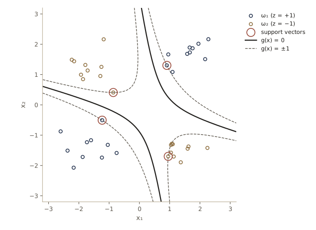
Multicategory generalizations
No single recipe extends every two-category procedure to \(c\) categories. The natural target is the linear machine of the first section, now with generalized discriminants \(g_i(\mathbf{x}) = \mathbf{a}_i^{t}\mathbf{y}\), \(i = 1, \dots, c\), assigning \(\mathbf{x}\) to \(\omega_i\) when \(g_i(\mathbf{x}) > g_j(\mathbf{x})\) for all \(j \ne i\). It is the multicategory analog of the two-class discriminant and it matches the Gaussian results of module 02. A set of labeled samples, with \(\mathcal{Y}_i\) the samples of \(\omega_i\), is linearly separable in the multicategory sense if some linear machine classifies all of them correctly: there are \(\hat{\mathbf{a}}_1, \dots, \hat{\mathbf{a}}_c\) with
\[\hat{\mathbf{a}}_i^{t}\mathbf{y} > \hat{\mathbf{a}}_j^{t}\mathbf{y} \qquad \text{for every } \mathbf{y} \in \mathcal{Y}_i \text{ and every } j \ne i .\]Our example has four classes in the plane, 25 samples each.
rng_mc = np.random.default_rng(68)
means_mc = np.array([[0.0, 3.0], [3.0, 0.5], [0.0, -2.5], [-3.0, 0.5]])
X_mc = np.vstack([rng_mc.normal(m, 0.8, size=(25, 2)) for m in means_mc])
lab_mc = np.repeat(np.arange(4), 25)
Y_mc = augment(X_mc)
c_mc, dh_mc = 4, Y_mc.shape[1]
Kesler’s construction
The separability condition is a set of linear inequalities in the stacked weight vector, and a rearrangement turns it into a two-category problem. Suppose \(\mathbf{y} \in \mathcal{Y}_1\). The \(c - 1\) inequalities \(\hat{\mathbf{a}}_1^{t}\mathbf{y} - \hat{\mathbf{a}}_j^{t}\mathbf{y} > 0\), \(j = 2, \dots, c\), say that the \(c\hat{d}\)-dimensional vector
\[\hat{\boldsymbol{\alpha}} = \begin{pmatrix} \hat{\mathbf{a}}_1 \\ \vdots \\ \hat{\mathbf{a}}_c \end{pmatrix} \quad \text{satisfies} \quad \hat{\boldsymbol{\alpha}}^{t}\boldsymbol{\eta}_{1j} > 0, \qquad \boldsymbol{\eta}_{12} = \begin{pmatrix} \mathbf{y} \\ -\mathbf{y} \\ \mathbf{0} \\ \vdots \\ \mathbf{0} \end{pmatrix}, \; \boldsymbol{\eta}_{13} = \begin{pmatrix} \mathbf{y} \\ \mathbf{0} \\ -\mathbf{y} \\ \vdots \\ \mathbf{0} \end{pmatrix}, \; \dots\]In general, for \(\mathbf{y} \in \mathcal{Y}_i\) and each \(j \ne i\), build \(\boldsymbol{\eta}_{ij}\) by splitting a \(c\hat{d}\)-vector into \(c\) blocks of length \(\hat{d}\), putting \(\mathbf{y}\) in block \(i\), \(-\mathbf{y}\) in block \(j\), and zeros elsewhere. Each \(\boldsymbol{\eta}_{ij}\) plays the role of a “normalized” two-class sample. Then the linear machine \(\hat{\mathbf{a}}_1, \dots, \hat{\mathbf{a}}_c\) classifies every sample correctly exactly when the single vector \(\hat{\boldsymbol{\alpha}}\) satisfies \(\hat{\boldsymbol{\alpha}}^{t}\boldsymbol{\eta} > 0\) for all \((c-1)n\) of the \(\boldsymbol{\eta}\)’s. This is Kesler’s construction. It multiplies the dimension by \(c\) and the number of samples by \(c - 1\), so it is not a practical training method; its value is that it turns every two-category convergence proof for error-correcting rules into a multicategory one.
def kesler_vectors(Y, labels, c):
    """One c*d_hat vector per (sample y of class i, class j != i): +y in block i, -y in block j."""
    n, dh = Y.shape
    rows = []
    for y, i in zip(Y, labels):
        for j in range(c):
            if j != i:
                eta = np.zeros(c * dh)
                eta[i * dh:(i + 1) * dh] = y
                eta[j * dh:(j + 1) * dh] = -y
                rows.append(eta)
    return np.array(rows)

E_mc = kesler_vectors(Y_mc, lab_mc, c_mc)
print(f"Kesler samples: {E_mc.shape[0]} vectors of dimension {E_mc.shape[1]}")

A_rand = rng_mc.normal(size=(dh_mc, c_mc))                    # any linear machine (columns a_i)
alpha_rand = A_rand.T.ravel()                                  # stacked (a_1; ...; a_c)
machine_ok = linear_machine(A_rand, X_mc) == lab_mc
kesler_ok = (E_mc @ alpha_rand > 0).reshape(-1, c_mc - 1).all(axis=1)
print(f"random machine: per-sample verdicts agree for all {np.sum(machine_ok == kesler_ok)} samples")
Kesler samples: 300 vectors of dimension 12
random machine: per-sample verdicts agree for all 100 samples
For a random machine, a sample is classified correctly exactly when all of its \(c - 1\) Kesler vectors are on the positive side, sample by sample.
Convergence of the fixed-increment rule
Now the multicategory version of the fixed-increment rule. Cycle through the samples; when \(\mathbf{y}^k \in \mathcal{Y}_i\) is misclassified, there is at least one \(j \ne i\) with \(\mathbf{a}_i(k)^{t}\mathbf{y}^k \le \mathbf{a}_j(k)^{t}\mathbf{y}^k\) (take the class with the largest discriminant). Correct the machine by
\[\mathbf{a}_i(k+1) = \mathbf{a}_i(k) + \mathbf{y}^k, \qquad \mathbf{a}_j(k+1) = \mathbf{a}_j(k) - \mathbf{y}^k, \qquad \mathbf{a}_l(k+1) = \mathbf{a}_l(k) \text{ for } l \ne i, j :\]reward the correct class, penalize the wrongly chosen one, leave the rest alone.
The convergence proof is one sentence once we look through Kesler’s lens. Stack the machine into \(\boldsymbol{\alpha}(k)\). The misclassification means \(\boldsymbol{\alpha}(k)^{t}\boldsymbol{\eta}_{ij} \le 0\) for the Kesler vector \(\boldsymbol{\eta}_{ij}\) built from \(\mathbf{y}^k\), and the correction is exactly \(\boldsymbol{\alpha}(k+1) = \boldsymbol{\alpha}(k) + \boldsymbol{\eta}_{ij}\). So the multicategory rule is the two-category fixed-increment rule on the Kesler samples, and by the perceptron convergence theorem it makes finitely many corrections and ends at a machine that classifies every sample correctly — provided the samples are linearly separable. The same translation extends the variable-increment and relaxation results to linear machines. It does not help much with MSE or linear programming, whose criteria do not decompose this way.
def linear_machine_fixed_increment(Y, labels, c, max_passes=10000):
    """Fixed-increment rule for a linear machine. Returns (A with columns a_i, corrections, passes)."""
    A = np.zeros((Y.shape[1], c))
    corrections = 0
    for p in range(1, max_passes + 1):
        changed = False
        for y, i in zip(Y, labels):
            g = y @ A
            g_other = np.where(np.arange(c) == i, -np.inf, g)
            j = np.argmax(g_other)                          # strongest competitor
            if g[j] >= g[i]:                                 # misclassified (ties count)
                A[:, i] += y                                 # reward the true class
                A[:, j] -= y                                 # penalize the winner
                corrections += 1
                changed = True
        if not changed:
            return A, corrections, p
    return A, corrections, None

A_fi, corr_mc, passes_mc = linear_machine_fixed_increment(Y_mc, lab_mc, c_mc)
alpha_fi = A_fi.T.ravel()
print(f"linear machine: {corr_mc} corrections in {passes_mc} passes; "
      f"training errors {np.sum(linear_machine(A_fi, X_mc) != lab_mc)}")
print(f"all Kesler vectors positive: {bool(np.all(E_mc @ alpha_fi > 0))}")

beta2_k = np.max(np.sum(E_mc**2, axis=1))                   # = 2 max ||y||^2
gamma_k = np.min(E_mc @ alpha_fi)
print(f"two-class bound in Kesler space, using this solution: "
      f"{beta2_k * (alpha_fi @ alpha_fi) / gamma_k**2:.0f}")

a_kes, corr_kes, _, passes_kes = fixed_increment(E_mc)       # the two-class rule on Kesler samples
A_kes = a_kes.reshape(c_mc, dh_mc).T
print(f"two-class rule on the {len(E_mc)} Kesler samples: {len(corr_kes)} corrections "
      f"in {passes_kes} passes")
print(f"its machine: training errors {np.sum(linear_machine(A_kes, X_mc) != lab_mc)}, "
      f"same as above: {np.allclose(A_kes, A_fi)}")
linear machine: 55 corrections in 22 passes; training errors 0
all Kesler vectors positive: True
two-class bound in Kesler space, using this solution: 12423
two-class rule on the 300 Kesler samples: 55 corrections in 22 passes
its machine: training errors 0, same as above: True
Both routes reach a machine with no training errors, after far fewer corrections than the two-class bound computed in Kesler space. Here they even end at exactly the same machine: the two-class rule on the Kesler samples is the linear-machine rule in disguise. (In general the two can differ in which violated inequality they correct first, since the Kesler run takes the competitors in a fixed order rather than the strongest one.)
Generalizations for MSE procedures
The simplest MSE extension treats the \(c\)-class problem as \(c\) two-class problems: find \(\mathbf{a}_i\) as the MSE solution of \(\mathbf{a}_i^{t}\mathbf{y} = 1\) for \(\mathbf{y} \in \mathcal{Y}_i\) and \(\mathbf{a}_i^{t}\mathbf{y} = -1\) for the rest. By the asymptotic result of the MSE section, for large \(n\) each \(\mathbf{a}_i^{t}\mathbf{y}\) approximates \(P(\omega_i \mid \mathbf{x}) - P(\text{not } \omega_i \mid \mathbf{x}) = 2P(\omega_i \mid \mathbf{x}) - 1\) in the mean-square sense. Two consequences: we may as well use targets 1 and 0, so that \(\mathbf{a}_i^{t}\mathbf{y}\) approximates \(P(\omega_i \mid \mathbf{x})\) itself; and it is reasonable to feed these discriminants into a linear machine, choosing the largest, rather than thresholding each at zero.
With all \(n\) samples (unnormalized) as the rows of \(\mathbf{Y}\), the weight vectors as the columns of the \(\hat{d} \times c\) matrix \(\mathbf{A} = [\mathbf{a}_1 \cdots \mathbf{a}_c]\), and the targets as the \(n \times c\) matrix \(\mathbf{B}\) whose row for a sample of \(\omega_i\) has a 1 in column \(i\) and zeros elsewhere, the \(c\) problems share one pseudoinverse:
\[\mathbf{A} = \mathbf{Y}^{\dagger}\mathbf{B},\]which minimizes \(\operatorname{tr}\left[(\mathbf{Y}\mathbf{A} - \mathbf{B})^{t}(\mathbf{Y}\mathbf{A} - \mathbf{B})\right]\), the sum of the \(c\) squared error lengths (and each of them separately). A further generalization brings in a loss matrix: if the row of \(\mathbf{B}\) for a sample of \(\omega_j\) is \(-(\lambda_{1j}, \dots, \lambda_{cj})\), with \(\lambda_{ij}\) the loss for deciding \(\omega_i\) when the truth is \(\omega_j\), then as \(n \to \infty\) the discriminants approximate \(-\sum_j \lambda_{ij}P(\omega_j \mid \mathbf{x}) = -R(\alpha_i \mid \mathbf{x})\), the negative conditional risk of module 02, and choosing the largest is the Bayes rule (DHS Problem 37). With zero–one loss the targets are \(\mathbf{B} - \mathbf{1}\mathbf{1}^{t}\), which only lowers every discriminant by the same constant.
The last cell fits the MSE linear machine and uses the same four-class data to measure the ambiguous regions promised in the first section. One-versus-rest uses the four MSE discriminants with \(\pm 1\) targets, each thresholded at zero on its own; pairwise uses six MSE discriminants, each fitted on the samples of its two classes only, and assigns \(\omega_i\) when \(\omega_i\) wins all three of its contests.
B_mc = np.eye(c_mc)[lab_mc]                                  # 0/1 targets
A_mse = np.linalg.lstsq(Y_mc, B_mc, rcond=None)[0]          # A = Y+ B
out = Y_mc @ A_mse
print(f"MSE linear machine: training errors {np.sum(np.argmax(out, axis=1) != lab_mc)};  "
      f"outputs sum to one: max deviation {np.abs(out.sum(axis=1) - 1).max():.1e}")
A_loss = np.linalg.lstsq(Y_mc, B_mc - 1.0, rcond=None)[0]   # zero-one loss targets -lambda
print(f"zero-one loss targets shift every discriminant by -1: "
      f"{np.allclose(Y_mc @ A_loss, out - 1.0)}")

g_axis = np.linspace(-6, 6, 241)
G_mc = np.array(np.meshgrid(g_axis, g_axis)).reshape(2, -1).T
ovr = augment(G_mc) @ np.linalg.lstsq(Y_mc, 2 * B_mc - 1, rcond=None)[0] > 0   # one-vs-rest claims
n_claims = ovr.sum(axis=1)
f_axis = np.linspace(-1.5, 1.5, 601)                          # a fine grid near the center for pairwise
G_fine = np.array(np.meshgrid(f_axis, f_axis)).reshape(2, -1).T
wins = np.zeros((len(G_fine), c_mc), dtype=int)
for i in range(c_mc):
    for j in range(i + 1, c_mc):
        pair = (lab_mc == i) | (lab_mc == j)
        a_ij = np.linalg.lstsq(Y_mc[pair], np.where(lab_mc[pair] == i, 1.0, -1.0), rcond=None)[0]
        g_ij = augment(G_fine) @ a_ij
        wins[:, i] += g_ij > 0
        wins[:, j] += g_ij < 0
print(f"one-vs-rest: claimed by no class {np.mean(n_claims == 0):.1%}, "
      f"by two or more {np.mean(n_claims >= 2):.1%}")
no_winner = wins.max(axis=1) < c_mc - 1
print(f"pairwise: no class wins all its contests on an area of {np.mean(no_winner) * 3.0**2:.4f} "
      f"(x1 from {G_fine[no_winner, 0].min():.2f} to {G_fine[no_winner, 0].max():.2f})")
scores = augment(G_mc) @ A_mse
ties = np.sum(scores == scores.max(axis=1, keepdims=True), axis=1) > 1
print(f"linear machine: undefined (exact ties) on {np.mean(ties):.1%} of the grid")
MSE linear machine: training errors 1;  outputs sum to one: max deviation 4.4e-16
zero-one loss targets shift every discriminant by -1: True
one-vs-rest: claimed by no class 7.8%, by two or more 51.7%
pairwise: no class wins all its contests on an area of 0.0109 (x1 from -0.53 to 0.35)
linear machine: undefined (exact ties) on 0.0% of the grid
The MSE linear machine classifies the training set almost perfectly, and its outputs sum to one exactly, a general property of least squares with 1-of-\(c\) targets when the features include a constant (see Intro to ML, module 04 for the two-line proof). The two-class schemes leave regions without a unique answer. With one-versus-rest, more than half of the square \([-6, 6]^2\) is claimed by no class or by several, because a single line cannot cut one class away from three others well. The pairwise discriminants are nearly consistent on these symmetric data, but they still leave a small polygon near the center (area about 0.01) where no class wins all three of its contests. The linear machine answers everywhere; ties have probability zero.
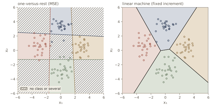
Summary
| Procedure | Criterion | Update or solution | Separable samples | Nonseparable samples |
|---|---|---|---|---|
| Fixed-increment perceptron | \(J_p = \sum_{\mathcal{Y}}(-\mathbf{a}^{t}\mathbf{y})\) | \(\mathbf{a} \leftarrow \mathbf{a} + \mathbf{y}^k\) when \(\mathbf{a}^{t}\mathbf{y}^k \le 0\) | finite convergence, at most \(\beta^2\lVert \hat{\mathbf{a}} \rVert^2/\gamma^2\) corrections | never stops; \(\lVert \mathbf{a} \rVert\) stays bounded |
| Variable increment with margin | \(\sum_{\mathcal{Y}}(b - \mathbf{a}^{t}\mathbf{y})\) | \(\mathbf{a} \leftarrow \mathbf{a} + \eta(k)\mathbf{y}^k\) when \(\mathbf{a}^{t}\mathbf{y}^k \le b\) | converges to \(\mathbf{a}^{t}\mathbf{y}_i > b\) under the \(\eta(k)\) conditions | with \(b > 0\) and decaying \(\eta\), settles near a reasonable \(\mathbf{a}\) |
| Relaxation with margin | \(J_r = \frac{1}{2}\sum_{\mathcal{Y}}\frac{(\mathbf{a}^{t}\mathbf{y} - b)^2}{\lVert \mathbf{y} \rVert^2}\) | move a fraction \(\eta \in (0, 2)\) of the way to \(\mathbf{a}^{t}\mathbf{y}^k = b\) | with \(b > 0\), reaches a solution vector in finitely many steps | never stops |
| Minimum squared error | \(J_s = \lVert \mathbf{Y}\mathbf{a} - \mathbf{b} \rVert^2\) | \(\mathbf{a} = \mathbf{Y}^{\dagger}\mathbf{b}\), or LMS: \(\mathbf{a} \leftarrow \mathbf{a} + \eta(k)(b_k - \mathbf{a}^{t}\mathbf{y}^k)\mathbf{y}^k\) | may not separate | always defined; Fisher’s direction for class-constant \(\mathbf{b}\); approximates \(g_0\) for \(\mathbf{b} = \mathbf{1}\) |
| Stochastic approximation | \(J_m = \mathcal{E}[(\mathbf{a}^{t}\mathbf{y} - \theta)^2]\) | LMS with \(\sum\eta = \infty\), \(\sum\eta^2 < \infty\), or recursive least squares | — | converges in mean square to the MSE approximation of the Bayes discriminant |
| Ho–Kashyap | \(\lVert \mathbf{Y}\mathbf{a} - \mathbf{b} \rVert^2\) over \(\mathbf{a}\) and \(\mathbf{b} > \mathbf{0}\) | \(\mathbf{b} \leftarrow \mathbf{b} + 2\eta\mathbf{e}^{+}\), \(\mathbf{a} = \mathbf{Y}^{\dagger}\mathbf{b}\), \(0 < \eta < 1\) | finite convergence to a separating vector | \(\mathbf{e} \le \mathbf{0}\), \(\mathbf{e} \ne \mathbf{0}\) proves nonseparability |
| Linear programming | \(\min\tau\), or \(\min\sum_i\tau_i\) (\(= J_p'\)) | simplex or another LP solver | finite; \(\tau = 0\) gives a solution | finite; proves nonseparability, or gives the global minimum of \(J_p'\) |
| Support vector machine | \(\min\frac{1}{2}\lVert \mathbf{w} \rVert^2\) s.t. \(z_kg(\mathbf{x}_k) \ge 1\) | dual quadratic program (SMO); kernels | maximum-margin hyperplane in \(\varphi\)-space | needs a soft margin (see Intro to ML, module 07) |
| Linear machine (multicategory) | Kesler’s construction | reward \(\mathbf{a}_i\), penalize \(\mathbf{a}_j\); or \(\mathbf{A} = \mathbf{Y}^{\dagger}\mathbf{B}\) | finite convergence (fixed increment) | MSE version approximates posteriors or conditional risks |
Ideas to carry forward:
- Training a linear classifier on separable data is solving a system of linear inequalities \(\mathbf{a}^{t}\mathbf{y}_i > 0\). The solution region is a convex cone in weight space, and a margin moves the search away from its boundary.
- Error-correcting rules (perceptron, relaxation) come with finite-convergence proofs on separable data and no stopping point otherwise. The proofs share one idea: every correction decreases the distance to some suitably chosen solution vector by a fixed amount.
- Squared error trades the separability guarantee for a criterion that is always well behaved and has a statistical meaning — Fisher’s direction, an approximation to the Bayes discriminant and to the posteriors. Ho–Kashyap and linear programming recover the separability test on top of it.
- Maximizing the margin controls complexity through how many support vectors there are, not how many weights, which is what makes very high-dimensional \(\varphi\)-mappings usable. Kesler’s construction reduces every multicategory error-correction rule to the two-category case.
Exercises
- Construct a four-class linear machine in the plane in which some pair of regions does not touch, and check your answer with the grid code of the first section. Then show that if the pairwise discriminants are taken to be the differences \(g_i - g_j\) of a single linear machine, the rule “choose the class that wins all its pairwise contests” agrees with the linear machine at every point, so the ambiguity measured at the end of the module comes entirely from training the pairwise discriminants independently.
- For the quadratic discriminant \(g(\mathbf{x}) = w_0 + \mathbf{w}^{t}\mathbf{x} + \mathbf{x}^{t}\mathbf{W}\mathbf{x}\) with \(\mathbf{W}\) invertible, carry out the shift of origin that removes the linear term and verify the expression for \(\overline{\mathbf{W}}\). For \(d = 2\), \(\mathbf{W} = \operatorname{diag}(1, -2)\), \(\mathbf{w} = (2, 0)^{t}\), \(w_0 = 1\), say what kind of curve \(g = 0\) is and sketch it.
- The bound \(k_0 = \beta^2\lVert \hat{\mathbf{a}} \rVert^2/\gamma^2\) holds for every solution vector \(\hat{\mathbf{a}}\), and is smallest for the one with the largest margin. Train
smowith the kernel \(K(\mathbf{x}, \mathbf{x}') = 1 + \mathbf{x}^{t}\mathbf{x}'\) (degree 1) on our separable two-class data, form \(\hat{\mathbf{a}} = (w_0, \mathbf{w})\) from its solution (the constant feature contributes to \(w_0\) too), and compute \(k_0\). Compare it with the bound froma_batchand with the 28 corrections the rule actually made. Why does even the best bound stay far above the actual count? - Run
variable_incrementon the separable data with \(b = 1\) and \(\eta(k) = 1\), \(k^{-1/2}\), \(k^{-1}\), and \(k^{-2}\), starting from \(\mathbf{a}(1) = (10, 10, 10)^{t}\), with at most 10,000 passes. Which runs reach a solution? Show that with \(\eta(k) = k^{-2}\) the total distance the weight vector can ever travel is bounded, and use this to explain why such a schedule can fail from a distant start even though the samples are separable. - Prove the two identities used in the relation between MSE and Fisher’s discriminant, and show that the scalar \(c\) in \(\mathbf{S}_W\mathbf{w} = c(\mathbf{m}_1 - \mathbf{m}_2)\) is positive whenever \(\beta_1 + \beta_2 > 0\). (Hint: write \(\mathbf{w} = s\,\mathbf{S}_W^{-1}(\mathbf{m}_1 - \mathbf{m}_2)\) and solve for \(s\).)
- Repeat the asymptotic MSE experiment with degree 1, 3, 5, and 7 polynomial features. For each, report the mean-square error \(\epsilon^2(\mathbf{a}^{*})\) and the probability of error of the rule “decide \(\omega_1\) when \(\mathbf{a}^{*t}\mathbf{y} > 0\)”, both by numerical integration, and compare with the Bayes error. Does a smaller \(\epsilon^2\) always mean a smaller error rate?
- Show that for any \(\mathbf{Y}\) with \(\mathbf{Y}^{t}\mathbf{Y}\) nonsingular, \(\mathbf{Y}\mathbf{Y}^{\dagger}\) is symmetric and idempotent, and that \(\mathbf{I} - \mathbf{Y}\mathbf{Y}^{\dagger}\) is too. Use this to rederive the Ho–Kashyap decrease identity, and explain what goes wrong in the proof if \(\eta = 1\).
- Run
ho_kashyapon the overlapping Gaussians with \(\eta = 0.1, 0.5, 0.9\) and plot \(\lVert \mathbf{e}(k) \rVert^2\) and \(\lVert \mathbf{e}^{+}(k) \rVert^2\) against \(k\). How does the step at which nonseparability is declared depend on \(\eta\) and on the tolerance? Then take the final \(\mathbf{a}\) as a classifier and compare its training error with the MSE and linear-programming solutions. - The
smofunction already accepts the box constraint \(0 \le \alpha_k \le C\) of the soft-margin machine (read the clipping step to see how). Train it on the overlapping Gaussians with the kernel \(K(\mathbf{x}, \mathbf{x}') = \mathbf{x}^{t}\mathbf{x}'\) for \(C = 0.01, 1, 100\). Report the number of support vectors, how many have \(\alpha_k = C\), and the training error, and relate the results to the leave-one-out bound. - Implement the multicategory relaxation rule suggested by Kesler’s construction (single-sample relaxation on the \(\boldsymbol{\eta}_{ij}\), translated back into updates of \(\mathbf{a}_i\) and \(\mathbf{a}_j\)) and compare its number of corrections with the fixed-increment linear machine on our four-class data for several \(\eta\).
- Use
lp_perceptron_criterionon our separable data with margins \(b = 1\) and \(b = 10\). Are the solutions separating? How do their geometric margins (smallest distance of a sample to the boundary in \(\mathbf{x}\)-space) compare with the fixed-increment and support vector solutions? - In your own words: the perceptron, MSE, and Ho–Kashyap procedures all adjust a linear discriminant, yet they respond very differently to a cluster of samples that is correctly classified by a wide margin. Explain why, in terms of their criterion functions, and say which behavior you would want in an application where some training samples may be mislabeled.
Going further
- R. O. Duda, P. E. Hart, and D. G. Stork, Pattern Classification, 2nd ed., chapter 5 — the source for this module. Problems 2–6 (linear machines and separability), 12 (quadratic surfaces), 13–14 (gradient descent), 15–19 (perceptron convergence and its variants), 20 (relaxation), 21–26 (MSE, Fisher, stochastic approximation, LMS), 27 (Ho–Kashyap), 28 (linear programming), 29–34 (support vector machines), and 35–38 (multicategory procedures) pair with the sections above, as do Computer exercises 1–12, one or more per section.
- F. Rosenblatt, “The perceptron: a probabilistic model for information storage and organization in the brain”, Psychological Review, 1958 — the origin of the perceptron.
- Y.-C. Ho and R. L. Kashyap, “An algorithm for linear inequalities and its applications,” IEEE Transactions on Electronic Computers, 1965 — the Ho–Kashyap procedure. In the same journal and year, T. M. Cover’s “Geometrical and statistical properties of systems of linear inequalities with applications in pattern recognition” proves the counting theorem we tested with linear programming.
- C. Cortes and V. Vapnik, “Support-vector networks”, Machine Learning, 1995 — the soft-margin support vector machine. J. Platt’s 1998 Microsoft Research technical report “Sequential minimal optimization: a fast algorithm for training support vector machines” introduced SMO.
- The machine learning notes cover the same ground from the probabilistic side: Intro to ML, module 04 (least squares, Fisher, the perceptron, logistic regression) and Intro to ML, module 07 (support vector machines with soft margins, and relevance vector machines). In this course, module 06 stacks linear discriminants into networks that learn their own \(\varphi\)-functions, and module 09 takes up leave-one-out estimates and the question of how much a small training error is worth.
These notes follow the chapters of R. O. Duda, P. E. Hart, and D. G. Stork, Pattern Classification, 2nd edition (Wiley, 2001), the course text. The explanations, code, figures, and exercises here are written for this course; the book remains the reference, with the full derivations, worked examples, and many more problems.