CSE 455/555 · Module 06 · Session 6
Multilayer Neural Networks
Feedforward networks and their expressive power, backpropagation built from scratch, error surfaces, outputs as posterior probabilities, practical training techniques, second-order methods, and pruning.
Companion reading: Duda, Hart & Stork, Pattern Classification, chapter 6, “Multilayer Neural Networks”
By the end of this module you can
- Compute the feedforward operation of a \(d\)-\(n_H\)-\(c\) network by hand and in NumPy, and build a three-layer network of threshold units that solves XOR.
- State Kolmogorov’s representation theorem and the universal-approximation idea, and explain why neither tells us how to find weights from data.
- Derive the backpropagation updates for hidden-to-output and input-to-hidden weights from the sensitivities, and verify them with a finite-difference gradient check.
- Implement stochastic, batch, and on-line training, read learning curves for training, validation, and test data, and use a validation set to stop training.
- Describe the error surface of small networks, find several different minima of the XOR problem from different starting weights, and show how hidden units remap the inputs into a linearly separable representation.
- Show that a network trained on squared error with 0–1 targets approximates the posterior probabilities, compare its outputs with true posteriors, and train softmax outputs with a cross-entropy criterion.
- Choose the activation function, input scaling, targets, initial weights, learning rate, momentum, weight decay, and number of hidden units with a reason for each choice.
- Implement Newton’s method, Quickprop, and conjugate gradient descent, build a radial basis function network, and rank weights for pruning with Optimal Brain Damage and Optimal Brain Surgeon.
Contents
- From linear machines to multilayer networks
- Feedforward operation and classification
- The backpropagation algorithm
- Error surfaces
- Backpropagation as feature mapping
- Backpropagation, Bayes theory, and probability
- Related statistical techniques
- Practical techniques for improving backpropagation
- Second-order methods
- Additional networks and training methods
- Regularization, complexity adjustment, and pruning
- Summary
- Exercises
- Going further
In module 05 we trained linear machines: a weight vector, a bias, and a decision rule based on the sign of \(\mathbf{a}^{t}\mathbf{y}\). The perceptron, relaxation, and LMS procedures all came with guarantees, and LMS even gave a least-squares approximation to the Bayes discriminant of module 02. Their weakness is the one we met at the end of that module: the decision boundaries are hyperplanes, or hyperplanes in a space of nonlinear functions \(\varphi\) that we had to pick in advance.
This module follows chapter 6 of Duda, Hart & Stork (DHS). A multilayer neural network learns the nonlinear functions and the linear discriminant at the same time. It is still a linear machine at its output, but the space it works in is produced by a layer of adjustable nonlinear units. We build such networks from scratch in NumPy, derive the backpropagation algorithm that trains them by gradient descent, look at their error surfaces and at what the hidden units learn, show that their outputs approximate posterior probabilities, and then work through the long list of practical techniques and faster training methods that DHS collect.
The Intro to ML notes build backpropagation in Bishop’s notation in Intro to ML, module 05, with a longer treatment of the Hessian and of Bayesian networks. Here we give a compact but complete derivation in DHS’s notation and spend more time on what DHS emphasize: the network as a discriminant function, the link to Bayes decision theory, and the heuristics that make training work.
From linear machines to multilayer networks
A linear machine can only draw hyperplanes. We could make it more flexible by mapping \(\mathbf{x}\) through fixed nonlinear functions first, but a complete basis such as all polynomials has far too many parameters for a finite training set, and prior knowledge rarely tells us exactly which functions to use. What we want is a family of nonlinear functions with a modest number of parameters that can be learned from the data along with the discriminant.
A multilayer network does this by stacking units. Each unit forms a weighted sum of its inputs and passes it through a fixed nonlinearity; the units of one layer feed the next. The key practical fact is that the resulting function is differentiable in all its weights, so gradient descent can adjust every weight at once. Backpropagation is the bookkeeping that computes that gradient, and it reduces to the LMS rule of module 05 when there is no hidden layer.
A word on counting. DHS count layers of units: a network with an input layer, one hidden layer, and an output layer is a three-layer network, and the linear machines of module 05 are two-layer networks. The ML notes count layers of adaptive weights and call the same network a two-layer network. Both conventions are common; we follow DHS here. We also use DHS’s transpose \(\mathbf{w}^{t}\) and classes \(\omega_1, \dots, \omega_c\), where the ML notes write \(\mathbf{w}^{\mathrm{T}}\) and \(\mathcal{C}_k\).
The first cell sets up NumPy and a few helpers that the whole module uses: activation functions packaged with their derivatives, and a function that prepends the constant input \(x_0 = 1\) so that a bias is just one more weight.
import numpy as np
from collections import namedtuple
from scipy.special import expit, softmax, logsumexp
from scipy.stats import norm

np.set_printoptions(precision=4, suppress=True)
rng = np.random.default_rng(606)

Act = namedtuple("Act", ["name", "f", "df"])     # an activation function and its derivative

A_TANH, B_TANH = 1.716, 2.0 / 3.0                # f(net) = a tanh(b net), a and b explained later
TANH = Act("tanh", lambda net: A_TANH * np.tanh(B_TANH * net),
           lambda net: A_TANH * B_TANH * (1.0 - np.tanh(B_TANH * net) ** 2))
LOGISTIC = Act("logistic", expit, lambda net: expit(net) * (1.0 - expit(net)))
LINEAR = Act("linear", lambda net: net, lambda net: np.ones_like(net))
SOFTMAX = Act("softmax", lambda net: softmax(net, axis=1), None)   # used only with cross-entropy

def sgn(net):
    """Threshold unit: +1 if net >= 0, otherwise -1."""
    return np.where(net >= 0, 1.0, -1.0)

def augment(X):
    """Prepend the constant input x_0 = 1 to every row (one row per pattern)."""
    return np.column_stack([np.ones(len(X)), X])

print(augment(np.array([[0.5, -2.0], [3.0, 1.0]])))
[[ 1.   0.5 -2. ]
 [ 1.   3.   1. ]]
Feedforward operation and classification
A network that computes XOR
The simplest problem a linear machine cannot solve is the exclusive-OR (XOR), or two-bit parity: with inputs \(x_1, x_2 \in \{-1, +1\}\), class \(\omega_1\) is the pair of points where the inputs differ and \(\omega_2\) the pair where they agree. The two classes sit on the two diagonals of a square, and no line separates them.
A three-layer network solves it. The input units just pass on the components of \(\mathbf{x}\). Each hidden unit \(j\) (hidden because neither the input nor the output shows its value) computes its net activation, the inner product of its weights with the augmented input,
\[net_j = \sum_{i=1}^{d} x_i w_{ji} + w_{j0} = \sum_{i=0}^{d} x_i w_{ji} = \mathbf{w}_j^{t}\mathbf{x},\]and emits \(y_j = f(net_j)\), where \(f\) is the activation function. Here \(w_{ji}\) is the weight on the connection from input unit \(i\) to hidden unit \(j\), and \(x_0 = 1\) carries the bias \(w_{j0}\). Each output unit \(k\) does the same with the hidden signals, again with a constant \(y_0 = 1\):
\[net_k = \sum_{j=0}^{n_H} y_j w_{kj} = \mathbf{w}_k^{t}\mathbf{y}, \qquad z_k = f(net_k),\]where \(n_H\) is the number of hidden units. For now let every unit be a threshold unit, \(f(net) = \operatorname{sgn}(net)\), which is \(+1\) when \(net \ge 0\) and \(-1\) otherwise.
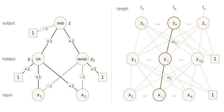
To build XOR from pieces a linear unit can compute, note that “the inputs differ” is the same as “at least one input is \(+1\)” AND “not both are \(+1\)”. So we let hidden unit 1 compute OR, hidden unit 2 compute NAND, and the output unit compute AND of the two:
- OR: \(net_1 = x_1 + x_2 + 1\), positive unless both inputs are \(-1\).
- NAND: \(net_2 = -x_1 - x_2 + 1\), positive unless both inputs are \(+1\).
- AND: \(net_k = y_1 + y_2 - 1\), positive only when both hidden units output \(+1\).
The cell below runs the four patterns through this 2-2-1 network and prints every intermediate quantity.
X_xor = np.array([[-1, -1], [-1, 1], [1, -1], [1, 1]], dtype=float)
t_xor = np.array([-1.0, 1.0, 1.0, -1.0])          # +1 = omega_1 (inputs differ)

W1_hand = np.array([[1.0,  1.0,  1.0],             # hidden unit 1 (OR):   w_10, w_11, w_12
                    [1.0, -1.0, -1.0]])            # hidden unit 2 (NAND): w_20, w_21, w_22
W2_hand = np.array([[-1.0, 1.0, 1.0]])             # output unit (AND):    w_k0, w_k1, w_k2

net_h = augment(X_xor) @ W1_hand.T                 # net_j = w_j^t x
Y = sgn(net_h)                                     # y_j = f(net_j)
net_o = augment(Y) @ W2_hand.T                     # net_k = w_k^t y
z = sgn(net_o)[:, 0]                               # z_k = f(net_k)
print("  x1  x2   net1 net2   y1  y2   net_k   z  target")
for x, nh, y_, no, zz, t in zip(X_xor, net_h, Y, net_o[:, 0], z, t_xor):
    print(f"{x[0]:4.0f}{x[1]:4.0f}  {nh[0]:5.0f}{nh[1]:5.0f}  {y_[0]:4.0f}{y_[1]:4.0f}  "
          f"{no:6.0f}  {zz:3.0f}  {t:5.0f}")
print("all four patterns correct:", bool(np.all(z == t_xor)))
  x1  x2   net1 net2   y1  y2   net_k   z  target
  -1  -1     -1    3    -1   1      -1   -1     -1
  -1   1      1    1     1   1       1    1      1
   1  -1      1    1     1   1       1    1      1
   1   1      3   -1     1  -1      -1   -1     -1
all four patterns correct: True
Each hidden unit is a perceptron with its own line in the \(x_1 x_2\)-plane; the output unit is a perceptron in the \(y_1 y_2\)-plane of hidden outputs. In that plane the four patterns land on only three points, \((1, -1)\), \((1, 1)\), and \((-1, 1)\), and the two \(\omega_1\) patterns share the point \((1, 1)\), which a single line cuts off from the other two. The hidden layer has made the problem linearly separable. That is the whole idea of this module in miniature; the rest is about finding such weights automatically.
General feedforward operation
Nothing in the construction depends on having two inputs, two hidden units, or one output. With \(d\) inputs, \(n_H\) hidden units, and \(c\) outputs, one per class, output \(k\) computes the discriminant function
\[g_k(\mathbf{x}) \equiv z_k = f\left( \sum_{j=1}^{n_H} w_{kj}\, f\left( \sum_{i=1}^{d} w_{ji} x_i + w_{j0} \right) + w_{k0} \right),\]and we classify \(\mathbf{x}\) into the class whose discriminant is largest, exactly as in module 02. With two classes it is customary to use one output and read the class from its sign. The activation functions need not be sign functions; for training we want them differentiable, and the output units may use a different \(f\) from the hidden units. This is the class of functions a three-layer network implements, and a \(d\)-\(n_H\)-\(c\) network has \((d+1)n_H + (n_H+1)c\) weights.
In code we store the input-to-hidden weights as a matrix W1 of shape \((n_H, d+1)\) whose row \(j\) is \(\mathbf{w}_j\) (bias first), and the hidden-to-output weights as W2 of shape \((c, n_H+1)\). Processing all \(n\) patterns at once is then two matrix products. The initializer draws weights uniformly from a range that we justify later, in the section on initializing weights.
def init_weights(d, n_H, c, rng, scale=1.0):
    """Uniform initial weights: input-to-hidden in +-1/sqrt(d), hidden-to-output in +-1/sqrt(n_H)."""
    W1 = scale * rng.uniform(-1, 1, (n_H, d + 1)) / np.sqrt(d)
    W2 = scale * rng.uniform(-1, 1, (c, n_H + 1)) / np.sqrt(n_H)
    return W1, W2

def forward(W1, W2, X, hid=TANH, out=TANH):
    """Feedforward operation for all rows of X: returns net_j, y_j, net_k, z_k (each n x units)."""
    net_h = augment(X) @ W1.T          # net_j = w_j^t x
    Y = hid.f(net_h)                   # y_j = f(net_j)
    net_o = augment(Y) @ W2.T          # net_k = w_k^t y
    return net_h, Y, net_o, out.f(net_o)

def classify(W1, W2, X, hid=TANH, out=TANH):
    """Class index 0..c-1: sign of a single output (+ -> 0), else the largest output."""
    Z = forward(W1, W2, X, hid, out)[3]
    return (Z[:, 0] < 0).astype(int) if Z.shape[1] == 1 else Z.argmax(axis=1)

d, n_H, c = 4, 5, 3
W1, W2 = init_weights(d, n_H, c, rng)
net_h, Y, net_o, Z = forward(W1, W2, rng.standard_normal((6, d)))
print("shapes:", net_h.shape, Y.shape, net_o.shape, Z.shape)
print("number of weights:", W1.size + W2.size, "=", (d + 1) * n_H + (n_H + 1) * c)
shapes: (6, 5) (6, 5) (6, 3) (6, 3)
number of weights: 43 = 43
Expressive power of multilayer networks
How much can a three-layer network represent? The answer is: any continuous function, given enough hidden units. The oldest result of this kind is Kolmogorov’s theorem (1957): every continuous function \(g(\mathbf{x})\) on the unit hypercube \([0, 1]^d\), \(d \ge 2\), can be written exactly as
\[g(\mathbf{x}) = \sum_{j=1}^{2d+1} \Xi_j\left( \sum_{i=1}^{d} \psi_{ij}(x_i) \right)\]for suitable continuous one-variable functions \(\Xi_j\) and \(\psi_{ij}\). Read as a network, there are \(2d+1\) hidden units, each receiving a sum of nonlinear functions of the individual inputs and emitting a nonlinear function of that sum, and the output adds up the hidden units. Any bounded feature space can be rescaled into the unit cube, so the domain is no restriction.
The theorem is a statement about existence, and its connection to practical networks is loose. The inner functions \(\psi_{ij}\) are not weighted sums followed by a sigmoid; they are wild, nowhere near smooth, and cannot be made smooth in general. And the theorem says nothing about how to find the functions from training data, which is the actual problem.
A more useful picture is the universal approximation idea. A pair of steep sigmoids in opposition, \(\tfrac12[\tanh(s(x - a)) - \tanh(s(x - b))]\), is a bump that is close to 1 on \([a, b]\) and close to 0 elsewhere. Two hidden units make one bump, and a linear output unit can add bumps of any heights. With enough bumps we can follow any continuous function of one variable as closely as we like; in more dimensions, bumps can be built from more sigmoids, and theorems from the late 1980s make the argument rigorous for sigmoid hidden units. The cell builds this construction for a function of our choosing and measures how the error falls as we add hidden units.
def g_target(x):
    return np.sin(3 * np.pi * x) * np.exp(-x) + x

def bump_network(x, g, K):
    """A 1-2K-1 network: K bumps of width 1/K, each made of two steep tanh units, heights g(center)."""
    edges = np.linspace(0, 1, K + 1)
    centers = 0.5 * (edges[:-1] + edges[1:])
    s = 20.0 * K                                            # steepness grows with K
    bumps = 0.5 * (np.tanh(s * (x[:, None] - edges[:-1])) - np.tanh(s * (x[:, None] - edges[1:])))
    return bumps @ g(centers)                              # linear output unit

x = np.linspace(0.05, 0.95, 2001)
for K in [5, 10, 20, 40, 80]:
    err = np.abs(bump_network(x, g_target, K) - g_target(x))
    print(f"hidden units = {2 * K:4d}   max error = {err.max():.4f}   mean error = {err.mean():.4f}")
hidden units =   10   max error = 0.4489   mean error = 0.1561
hidden units =   20   max error = 0.2859   mean error = 0.0773
hidden units =   40   max error = 0.1464   mean error = 0.0386
hidden units =   80   max error = 0.0778   mean error = 0.0193
hidden units =  160   max error = 0.0395   mean error = 0.0096
The maximum error roughly halves each time the number of bumps doubles, as it should for a staircase approximation of a smooth function. Two cautions. First, trained networks do not build their functions this way: backpropagation never discovers neat Fourier-like sums or tidy pairs of opposing sigmoids. Second, the construction needs to know the function, and in pattern recognition the function (the posterior, say) is exactly what we do not know. Results on expressive power tell us that a three-layer network is flexible enough; they say nothing about how many hidden units a real problem needs or how to set the weights. The decision regions of a network need not be convex or even connected, which is what we need to hope for good performance on hard problems.
The backpropagation algorithm
Setting the hidden-to-output weights is the easy half of training: if the hidden outputs \(y_j\) were fixed, the output layer would be a linear machine and LMS would train it. The hard half is the input-to-hidden weights. No teacher tells us what a hidden unit ought to output, so we cannot form an error at a hidden unit directly. This is the credit assignment problem: when the output is wrong, how much of the blame belongs to each hidden unit, and to each of its weights? Backpropagation answers it by computing an effective error for every hidden unit from the errors at the outputs.
A network has two modes of operation. In feedforward operation, a pattern is presented to the inputs and the signals pass layer by layer to the outputs. In learning, the outputs are compared with the desired target values and the weights are changed to bring the outputs closer to them.
Network learning
For one pattern with target vector \(\mathbf{t}\) and network output \(\mathbf{z}\), both of length \(c\), the training error is the squared error
\[J(\mathbf{w}) = \frac{1}{2} \sum_{k=1}^{c} (t_k - z_k)^2 = \frac{1}{2} \lVert \mathbf{t} - \mathbf{z} \rVert^2 ,\]where \(\mathbf{w}\) stands for all the weights in the network. Backpropagation is gradient descent on \(J\): starting from random weights, it changes each weight against its derivative,
\[\Delta w_{pq} = -\eta \frac{\partial J}{\partial w_{pq}}, \qquad \mathbf{w}(m+1) = \mathbf{w}(m) + \Delta \mathbf{w}(m),\]where \(\eta\) is the learning rate and \(m\) counts pattern presentations. All the work is in the derivatives, and the chain rule supplies them.
Hidden-to-output weights. The error depends on \(w_{kj}\) only through \(net_k\), so
\[\frac{\partial J}{\partial w_{kj}} = \frac{\partial J}{\partial net_k} \frac{\partial net_k}{\partial w_{kj}} = -\delta_k \frac{\partial net_k}{\partial w_{kj}},\]where we define the sensitivity of unit \(k\) as
\[\delta_k = -\frac{\partial J}{\partial net_k}.\]It measures how the error changes when the unit’s net activation changes (DHS include the minus sign so that \(\delta\) points downhill; Bishop’s \(\delta\) in the ML notes has the opposite sign). Differentiating \(J\) through \(z_k = f(net_k)\) gives
\[\delta_k = -\frac{\partial J}{\partial z_k} \frac{\partial z_k}{\partial net_k} = (t_k - z_k) f'(net_k),\]and since \(net_k = \sum_j w_{kj} y_j\), the last factor is \(\partial net_k / \partial w_{kj} = y_j\). So
\[\Delta w_{kj} = \eta\, \delta_k\, y_j = \eta\, (t_k - z_k)\, f'(net_k)\, y_j .\]With a linear output unit, \(f'(net_k) = 1\), and this is exactly the LMS rule of module 05.
Input-to-hidden weights. Now \(w_{ji}\) affects the error through \(y_j\), which feeds every output unit:
\[\frac{\partial J}{\partial w_{ji}} = \frac{\partial J}{\partial y_j} \frac{\partial y_j}{\partial net_j} \frac{\partial net_j}{\partial w_{ji}} .\]The first factor collects the effect of \(y_j\) on all \(c\) outputs:
\[\frac{\partial J}{\partial y_j} = -\sum_{k=1}^{c} (t_k - z_k) \frac{\partial z_k}{\partial y_j} = -\sum_{k=1}^{c} (t_k - z_k) f'(net_k)\, w_{kj} = -\sum_{k=1}^{c} w_{kj}\, \delta_k .\]The other two factors are \(f'(net_j)\) and \(x_i\). Defining the hidden unit’s sensitivity in the same way, \(\delta_j = -\partial J / \partial net_j\), we get
\[\delta_j = f'(net_j) \sum_{k=1}^{c} w_{kj}\, \delta_k, \qquad \Delta w_{ji} = \eta\, \delta_j\, x_i = \eta \left[ \sum_{k=1}^{c} w_{kj} \delta_k \right] f'(net_j)\, x_i .\]Result. Backpropagation for a three-layer network, one pattern:
- Feedforward: compute \(net_j\), \(y_j\), \(net_k\), \(z_k\).
- Output sensitivities: \(\delta_k = (t_k - z_k) f'(net_k)\).
- Hidden sensitivities, sent back through the same weights: \(\delta_j = f'(net_j) \sum_k w_{kj} \delta_k\).
- Updates: \(\Delta w_{kj} = \eta\, \delta_k y_j\) and \(\Delta w_{ji} = \eta\, \delta_j x_i\), with \(y_0 = x_0 = 1\) for the biases.
The hidden sensitivity is the solution to the credit assignment problem: each hidden unit is blamed in proportion to the output sensitivities, weighted by how strongly it connects to each output, and scaled by the slope of its own activation. The name comes from the second step, where errors flow backward through the network. At bottom, backpropagation is gradient descent in a layered model, with the chain rule applied through differentiable units.
The rules make intuitive sense. If \(z_k = t_k\) the output weights do not move. If the output is too small (\(t_k - z_k > 0\)) and \(y_j > 0\), then \(w_{kj}\) grows, which raises the output. If \(y_j = 0\), unit \(j\) cannot have contributed, and its weight to \(k\) does not change. They also explain why we must not start with all weights at zero: if every \(w_{kj}\) is zero, every \(\delta_j\) is zero and the input-to-hidden weights never move.
The derivation extends directly to networks with more layers (the sensitivity of each layer is computed from the one above), different activation functions per unit, direct input-to-output connections, or a separate learning rate per weight. Networks with feedback connections need more care; we return to them under recurrent networks.
Checking the gradient
In code we process all \(n\) patterns together and return the gradient of the total error \(\sum_m J_m\). The sensitivities become matrices with one row per pattern, and the sums over patterns of \(\delta_k y_j\) and \(\delta_j x_i\) become matrix products. The function also handles a second criterion, cross-entropy with softmax outputs, which we meet in the section on outputs as probabilities; for now read only the squared-error branch.
def criterion(Z, T, loss="sse"):
    """Squared error 1/2 sum ||t - z||^2, or cross-entropy -sum t ln z (softmax outputs)."""
    return 0.5 * np.sum((T - Z) ** 2) if loss == "sse" else -np.sum(T * np.log(Z + 1e-300))

def backprop(W1, W2, X, T, hid=TANH, out=TANH, loss="sse"):
    """Total training error over the rows of X and its gradient (dJ/dW1, dJ/dW2)."""
    net_h, Y, net_o, Z = forward(W1, W2, X, hid, out)
    if loss == "sse":
        delta_k = (T - Z) * out.df(net_o)             # delta_k = (t_k - z_k) f'(net_k)
    else:
        delta_k = T - Z                               # softmax + cross-entropy
    delta_j = hid.df(net_h) * (delta_k @ W2[:, 1:])   # delta_j = f'(net_j) sum_k w_kj delta_k
    gW2 = -delta_k.T @ augment(Y)                     # dJ/dw_kj = -sum_m delta_k y_j
    gW1 = -delta_j.T @ augment(X)                     # dJ/dw_ji = -sum_m delta_j x_i
    return criterion(Z, T, loss), gW1, gW2
Backpropagation code is easy to get subtly wrong, and a wrong gradient often still trains, just badly. The standard safeguard is a finite-difference gradient check: perturb each weight by \(\pm h\) and compare the central difference \([J(w_q + h) - J(w_q - h)]/(2h)\), which has error \(O(h^2)\), with the analytic derivative. To do that we need to flatten the two weight matrices into one vector and back.
def pack(W1, W2):
    return np.concatenate([W1.ravel(), W2.ravel()])

def unpack(w, d, n_H, c):
    k = n_H * (d + 1)
    return w[:k].reshape(n_H, d + 1), w[k:].reshape(c, n_H + 1)

def numerical_gradient(J_of_w, w, h=1e-6):
    g = np.zeros_like(w)
    for q in range(len(w)):
        e = np.zeros_like(w); e[q] = h
        g[q] = (J_of_w(w + e) - J_of_w(w - e)) / (2 * h)
    return g

d, n_H, c = 3, 4, 2
Xg = rng.standard_normal((5, d))
Tg = np.eye(c)[rng.integers(0, c, 5)]                 # 1-of-c targets
W1, W2 = init_weights(d, n_H, c, rng, scale=2.0)
for out, loss in [(TANH, "sse"), (LOGISTIC, "sse"), (SOFTMAX, "ce")]:
    J_of_w = lambda w: backprop(*unpack(w, d, n_H, c), Xg, Tg, out=out, loss=loss)[0]
    _, g1, g2 = backprop(W1, W2, Xg, Tg, out=out, loss=loss)
    g_bp, g_num = pack(g1, g2), numerical_gradient(J_of_w, pack(W1, W2))
    rel = np.max(np.abs(g_bp - g_num)) / np.max(np.abs(g_num))
    print(f"{out.name:8s} outputs, {loss}: {len(g_bp)} weights, max relative difference = {rel:.1e}")
tanh     outputs, sse: 26 weights, max relative difference = 6.6e-10
logistic outputs, sse: 26 weights, max relative difference = 5.2e-10
softmax  outputs, ce: 26 weights, max relative difference = 2.2e-10
The analytic and numerical gradients agree to within a relative difference of about \(10^{-9}\) for all three output types, which is as close as central differences with \(h = 10^{-6}\) can show. From here on we trust backprop.
Training protocols
Supervised training presents patterns whose labels we know, the training set, and nudges the weights to make the outputs more like the targets. How the patterns are presented defines three training protocols:
- In stochastic training, each step picks a pattern at random from the training set and updates the weights using that pattern’s gradient alone. It is called stochastic because the pattern, and hence the update, is a random variable.
- In batch training, all patterns are presented and their weight changes added up before the weights change. One update per pass.
- In on-line training, every pattern is used a single time, when it arrives, and then thrown away. Nothing is stored.
An epoch is one presentation of every pattern in the training set; for stochastic training we count \(n\) random presentations as an epoch. The total error over the training set is the sum of the per-pattern errors, \(J = \sum_{m=1}^{n} J_m\). A stochastic update may raise the error summed over all the patterns even as it lowers the error on its own pattern, but over many updates \(J\) goes down.
In code, batch training uses the gradient of the per-pattern average \(J/n\), so that the learning rate does not have to change with the size of the training set. The batch trainer also accepts momentum and weight decay, which we add later in the section on practical techniques (leave them at zero for now), and a list of extra data sets whose error it records every epoch.
def train_stochastic(W1, W2, X, T, eta, epochs, rng, hid=TANH, out=TANH):
    """Stochastic backpropagation: each update uses one randomly chosen pattern."""
    W1, W2 = W1.copy(), W2.copy()
    n, hist = len(X), []
    for r in range(epochs):
        for m in rng.integers(0, n, n):                  # n random presentations = one epoch
            _, g1, g2 = backprop(W1, W2, X[m:m+1], T[m:m+1], hid, out)
            W1 -= eta * g1; W2 -= eta * g2
        hist.append(backprop(W1, W2, X, T, hid, out)[0] / n)
    return W1, W2, np.array(hist)

def train_batch(W1, W2, X, T, eta, epochs, alpha=0.0, decay=0.0, hid=TANH, out=TANH,
                loss="sse", monitor=()):
    """Batch backpropagation on J/n, with optional momentum alpha and weight decay epsilon.
    hist[r] holds J/n on the training set and on each (X, T) in monitor before update r."""
    W1, W2 = W1.copy(), W2.copy()
    n = len(X)
    b1, b2 = np.zeros_like(W1), np.zeros_like(W2)        # previous weight changes
    hist = np.zeros((epochs, 1 + len(monitor)))
    for r in range(epochs):
        J, g1, g2 = backprop(W1, W2, X, T, hid, out, loss)
        hist[r, 0] = J / n
        for s, (Xs, Ts) in enumerate(monitor):
            hist[r, s + 1] = criterion(forward(W1, W2, Xs, hid, out)[3], Ts, loss) / len(Xs)
        b1 = -eta * (1 - alpha) * g1 / n + alpha * b1
        b2 = -eta * (1 - alpha) * g2 / n + alpha * b2
        W1, W2 = (W1 + b1) * (1 - decay), (W2 + b2) * (1 - decay)
    return W1, W2, hist
We need a data set on which a linear machine fails. Our running example is a noisy XOR: each class is an equal mixture of two spherical Gaussians with standard deviation \(s\) at opposite corners of a square, \(\omega_1\) around \((1, 1)\) and \((-1, -1)\), \(\omega_2\) around \((1, -1)\) and \((-1, 1)\), with equal priors. Because it is our own construction we know its Bayes rule exactly. The class-conditional densities differ only through \(\cosh((x_1 + x_2)/s^2)\) versus \(\cosh((x_1 - x_2)/s^2)\), so the Bayes rule chooses \(\omega_1\) exactly when \(x_1 x_2 > 0\). A pattern from the Gaussian at \((1,1)\) is misclassified when exactly one coordinate changes sign, so with \(q = \Phi(-1/s)\) the Bayes error is \(2q(1-q)\). Labels in code are 0 for \(\omega_1\) and 1 for \(\omega_2\), and the single tanh output is trained toward \(+1\) for \(\omega_1\) and \(-1\) for \(\omega_2\).
def noisy_xor(n, rng, s=0.5):
    """Labels 0 (omega_1: corners (1,1), (-1,-1)) and 1 (omega_2: corners (1,-1), (-1,1))."""
    y = rng.integers(0, 2, n)
    corner = rng.choice([-1.0, 1.0], n)
    mean = np.column_stack([corner, np.where(y == 0, corner, -corner)])
    return mean + s * rng.standard_normal((n, 2)), y

def pm_targets(y):
    """Single-output targets: +1 for omega_1 (label 0), -1 for omega_2 (label 1)."""
    return np.where(y == 0, 1.0, -1.0)[:, None]

def xor_bayes_error(s):
    q = norm.cdf(-1.0 / s)
    return 2 * q * (1 - q)

X_nx, y_nx = noisy_xor(200, np.random.default_rng(1))      # training set, s = 0.5
X_nxt, y_nxt = noisy_xor(2000, np.random.default_rng(2))   # independent test set
T_nx = pm_targets(y_nx)
W1_0, W2_0 = init_weights(2, 4, 1, np.random.default_rng(4))

W1_s, W2_s, h_s = train_stochastic(W1_0, W2_0, X_nx, T_nx, eta=0.02, epochs=60,
                                   rng=np.random.default_rng(5))
W1_b, W2_b, h_b = train_batch(W1_0, W2_0, X_nx, T_nx, eta=0.5, epochs=60)
h_b = np.append(h_b[1:, 0], backprop(W1_b, W2_b, X_nx, T_nx)[0] / 200)   # J/n after each epoch
for r in [1, 5, 20, 60]:
    print(f"after {r:2d} epochs   J/n stochastic = {h_s[r-1]:.4f}   batch = {h_b[r-1]:.4f}")
for name, (A, B) in [("stochastic", (W1_s, W2_s)), ("batch", (W1_b, W2_b))]:
    print(f"{name:10s} test error = {np.mean(classify(A, B, X_nxt) != y_nxt):.3f}")
print(f"Bayes error = {xor_bayes_error(0.5):.3f}")
after  1 epochs   J/n stochastic = 0.4651   batch = 0.5256
after  5 epochs   J/n stochastic = 0.1276   batch = 0.4698
after 20 epochs   J/n stochastic = 0.0826   batch = 0.4608
after 60 epochs   J/n stochastic = 0.0693   batch = 0.0893
stochastic test error = 0.049
batch      test error = 0.057
Bayes error = 0.044
With the same starting weights, both protocols reach a similar network, with test errors close to the Bayes error, but stochastic training gets there in far fewer epochs: it makes \(n = 200\) small updates per epoch where batch training makes one. Per epoch the costs are comparable, so on this problem stochastic training is much faster. We return to this comparison in the section on on-line, stochastic, or batch training.
On-line training is what we do when patterns arrive in a stream that we cannot or do not want to store. The next cell feeds 3000 fresh patterns through the network once each, in order of arrival, and checks the test error along the way. After about a thousand patterns the network is as good as the ones trained on the stored set, and it never needed to keep more than one pattern in memory.
stream_rng = np.random.default_rng(6)
W1, W2 = W1_0.copy(), W2_0.copy()
for m in range(1, 3001):
    x_m, y_m = noisy_xor(1, stream_rng)                 # a new pattern, used once
    _, g1, g2 = backprop(W1, W2, x_m, pm_targets(y_m))
    W1 -= 0.02 * g1; W2 -= 0.02 * g2
    if m in (100, 300, 1000, 3000):
        print(f"{m:5d} patterns seen   test error = {np.mean(classify(W1, W2, X_nxt) != y_nxt):.3f}")
  100 patterns seen   test error = 0.437
  300 patterns seen   test error = 0.317
 1000 patterns seen   test error = 0.058
 3000 patterns seen   test error = 0.050
Learning curves
A learning curve plots the error, usually the average per pattern, against the amount of training. On the training set it typically falls steadily, especially in batch training with a modest learning rate, which is true gradient descent (momentum can add a small bump early on, as in the figure below). It levels off at a value set by how much the classes overlap (the Bayes error), how many training patterns there are, and how expressive the network is.
Two other data sets, independent of the training set, play different roles. A test set estimates how well the finished network will do on new patterns. A validation set is used during training to decide when to stop. The error on either is nearly always above the training error; it usually falls at first but can rise again once the network starts fitting peculiarities of its particular training patterns.
To see this we make the problem harder: noisier classes (\(s = 0.7\)), only 60 training patterns, and a network with 10 hidden units, far more than the problem needs.
s_lc = 0.7
X_tr, y_tr = noisy_xor(60, np.random.default_rng(11), s_lc)
X_va, y_va = noisy_xor(60, np.random.default_rng(12), s_lc)
X_te, y_te = noisy_xor(2000, np.random.default_rng(13), s_lc)
W1_lc0, W2_lc0 = init_weights(2, 10, 1, np.random.default_rng(3))
W1_lc, W2_lc, h_lc = train_batch(W1_lc0, W2_lc0, X_tr, pm_targets(y_tr), eta=0.2, epochs=3000,
                                 alpha=0.9, monitor=[(X_va, pm_targets(y_va)), (X_te, pm_targets(y_te))])
r_stop = int(np.argmin(h_lc[:, 1]))                    # epoch of minimum validation error
for r in [0, 50, r_stop, 1000, 2999]:
    tr, va, te = h_lc[r]
    print(f"epoch {r:4d}   J/n train = {tr:.3f}   validation = {va:.3f}   test = {te:.3f}")
print("validation minimum at epoch", r_stop)
epoch    0   J/n train = 0.588   validation = 0.614   test = 0.566
epoch   50   J/n train = 0.337   validation = 0.460   test = 0.398
epoch  136   J/n train = 0.132   validation = 0.237   test = 0.251
epoch 1000   J/n train = 0.074   validation = 0.302   test = 0.294
epoch 2999   J/n train = 0.069   validation = 0.305   test = 0.298
validation minimum at epoch 136
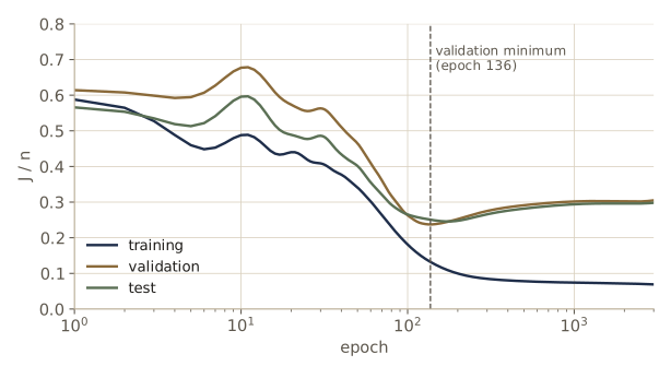
The training error falls throughout, but the validation error bottoms out early and climbs from there, and the test error follows the validation error closely. Stopping at the validation minimum is the idea behind stopped training, which we come back to among the practical techniques; the theory of validation and cross-validation is in module 09.
Error surfaces
Backpropagation is gradient descent on \(J(\mathbf{w})\), so the shape of that function, the error surface, governs how training behaves. Two features matter most. Local minima can trap gradient descent at a solution worse than the best one. Plateaus, regions where the error barely changes with the weights, make gradient descent crawl. Training usually starts with small weights, so the surface near \(\mathbf{w} = \mathbf{0}\) decides the initial direction of descent.
Some small networks
Consider the smallest nonlinear network, 1-1-1 with biases, on a one-dimensional two-class problem. If the classes are separable by a point, the error surface has a single low region, reached from almost any start, whose weights put the decision point between the classes. Away from it the surface is a set of terraces: large regions over which the steep sigmoids are saturated and the error stays constant, each terrace corresponding roughly to a fixed number of misclassified patterns. Moving along a terrace changes the weights but not the decision point, so the error does not change.
If the classes are not separable by a point, the lowest error is higher and there can be distinct low regions, for example one with the decision point on the left of an outlying pattern and one on its right. Keep in mind that the squared error is not the classification error: two weight settings that misclassify the same number of patterns can have different \(J\), because the outputs sit at different distances from their targets.
The exclusive-OR
The 2-2-1 network for XOR has nine weights, so its error surface lives in nine dimensions and we can only probe it. Each weight has a smaller share of the output than in a 1-1-1 network, so the surface varies more gently along any single weight, with ridges and valleys between the minima.
One way to probe it is to start gradient descent from many random weights and see where it ends. With the recommended initial range (the scale we derive later), every run we tried solves XOR. If we start with weights three times larger, many hidden units begin in saturation and some runs end elsewhere.
def train_xor(seed, n_H=2, scale=1.0, epochs=2000):
    W1, W2 = init_weights(2, n_H, 1, np.random.default_rng(seed), scale)
    return train_batch(W1, W2, X_xor, t_xor[:, None], eta=0.1, epochs=epochs, alpha=0.9)

def xor_summary(runs):
    J = np.array([h[-1, 0] for _, _, h in runs])
    correct = np.array([np.sum(sgn(forward(A, B, X_xor)[3][:, 0]) == t_xor) for A, B, _ in runs])
    return J, correct

for scale in [1.0, 3.0]:
    J, correct = xor_summary([train_xor(seed, scale=scale) for seed in range(20)])
    print(f"initial scale {scale}: solved (J/n < 1e-3) in {np.sum(J < 1e-3)} of 20 runs")
    for seed in np.flatnonzero(J >= 1e-3):
        print(f"   seed {seed:2d}: J/n = {J[seed]:.4f}, patterns correct = {correct[seed]}")
initial scale 1.0: solved (J/n < 1e-3) in 20 of 20 runs
initial scale 3.0: solved (J/n < 1e-3) in 15 of 20 runs
   seed  3: J/n = 0.2529, patterns correct = 2
   seed  4: J/n = 0.3310, patterns correct = 3
   seed  7: J/n = 0.2524, patterns correct = 2
   seed  9: J/n = 0.9217, patterns correct = 3
   seed 18: J/n = 0.2523, patterns correct = 2
What are these unsolved runs? A run can stall on a plateau and escape later, or it can sit in a local minimum. Continuing each of them to 8000 epochs tells the two cases apart, and the gradient norm shows how flat the surface is where they end.
for seed in [3, 4, 7, 9, 18]:
    W1, W2, h = train_xor(seed, scale=3.0, epochs=8000)
    _, g1, g2 = backprop(W1, W2, X_xor, t_xor[:, None])
    print(f"seed {seed:2d}: J/n at 2000 = {h[1999, 0]:.4f}, at 8000 = {h[-1, 0]:.4f}, "
          f"gradient norm = {np.sqrt(np.sum(g1**2) + np.sum(g2**2)):.1e}")
seed  3: J/n at 2000 = 0.2529, at 8000 = 0.2499, gradient norm = 1.0e-02
seed  4: J/n at 2000 = 0.3310, at 8000 = 0.0000, gradient norm = 4.9e-15
seed  7: J/n at 2000 = 0.2524, at 8000 = 0.2505, gradient norm = 4.1e-03
seed  9: J/n at 2000 = 0.9217, at 8000 = 0.0000, gradient norm = 7.3e-15
seed 18: J/n at 2000 = 0.2523, at 8000 = 0.0000, gradient norm = 7.0e-15
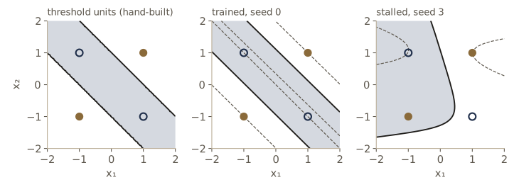
Three of the five (seeds 4, 9, and 18) were on plateaus: with enough extra epochs they find their way off and solve XOR exactly. Seeds 3 and 7 are still at \(J/n \approx 0.25\) after 8000 epochs, with two of the four patterns sitting on the boundary at \(z \approx 0\) (the right panel of the figure below). The error is still creeping down, so strictly speaking these runs may be descending an extremely flat valley rather than resting in a true minimum, but for training purposes the distinction does not matter: no practical amount of gradient descent gets them out.
The error surface is also symmetric. Relabeling the two hidden units (swapping the rows of W1 and the matching columns of W2) gives exactly the same function. Because \(f\) is odd, so does negating all the weights into a hidden unit together with its outgoing weights. Each solution therefore has \(2! \times 2^2 = 8\) equivalent copies, and so does each local minimum; a network with \(n_H\) hidden units has \(n_H!\, 2^{n_H}\) of them (exercise 3 asks you to check this numerically).
Larger networks
Intuition from two- and three-dimensional slices can mislead for large networks. With many weights the error varies slowly along any one of them, yet the surface can still have troughs, valleys, and canyons. Local minima behave differently in high dimensions: a barrier that blocks descent in a few dimensions may be avoidable through the others. As a rule, extra, superfluous weights make it less likely that training gets trapped, at the cost of a greater risk of overfitting (the subject of the last section). We can check the first half of that rule on XOR, starting again from the troublesome large initial weights but with more hidden units.
for n_H_try in [2, 4, 8]:
    J, _ = xor_summary([train_xor(seed, n_H=n_H_try, scale=3.0, epochs=1500) for seed in range(20)])
    print(f"n_H = {n_H_try}: unsolved in {np.sum(J >= 1e-3):2d} of 20 runs")
n_H = 2: unsolved in  6 of 20 runs
n_H = 4: unsolved in  0 of 20 runs
n_H = 8: unsolved in  0 of 20 runs
How important are multiple minima?
Local minima are one reason we train by iterative descent rather than hoping for an analytic solution: in a high-dimensional weight space there is no practical way to guarantee the global minimum. In practice we care about the error, not about globality. If training ends at a high error, the network has usually missed some structure in the problem, and the traditional remedy is to reinitialize the weights and train again, perhaps changing the learning rate or the number of hidden units. A local minimum with low error is usually acceptable, and since common stopping rules end training before any minimum is reached, convergence to the global minimum is not required for good performance.
Backpropagation as feature mapping
The hidden-to-output layer is a linear discriminant. Whatever extra power a multilayer network has over a linear machine must therefore come from the hidden layer, which warps the input space into a representation where a linear discriminant works. We can watch this happen by plotting, for every training pattern, the hidden-unit outputs \((y_1, y_2)\) of a 2-2-1 network as it learns the noisy XOR.
At the start the weights are small, each hidden unit operates in the nearly linear part of its sigmoid, and the map from \(\mathbf{x}\) to \(\mathbf{y}\) is close to linear. A linear map cannot turn XOR into a linearly separable problem. As training proceeds the input-to-hidden weights grow, the nonlinearity takes hold, and the classes pull apart. To measure separability in \(\mathbf{y}\)-space independently of the network’s own output unit, we fit the minimum-squared-error linear discriminant of module 05 to the hidden outputs and report its training error.
def mse_separability(Y, y):
    """Training error of the least-squares linear discriminant a^t (1, y) fitted to +-1 targets."""
    a = np.linalg.lstsq(augment(Y), pm_targets(y)[:, 0], rcond=None)[0]
    return np.mean((augment(Y) @ a < 0) != (y == 1))

W1_fm0, W2_fm0 = init_weights(2, 2, 1, np.random.default_rng(3))
for epochs in [0, 30, 100, 1500]:
    W1, W2, _ = train_batch(W1_fm0, W2_fm0, X_nx, T_nx, eta=0.2, epochs=epochs, alpha=0.9)
    Y = forward(W1, W2, X_nx)[1]
    print(f"epoch {epochs:4d}: linear error in y-space = {mse_separability(Y, y_nx):.3f},"
          f"  network training error = {np.mean(classify(W1, W2, X_nx) != y_nx):.3f}")
W1_fm, W2_fm = W1, W2
print("learned input-to-hidden weights (w_j0, w_j1, w_j2):")
print(W1_fm)
epoch    0: linear error in y-space = 0.565,  network training error = 0.515
epoch   30: linear error in y-space = 0.355,  network training error = 0.330
epoch  100: linear error in y-space = 0.115,  network training error = 0.130
epoch 1500: linear error in y-space = 0.090,  network training error = 0.095
learned input-to-hidden weights (w_j0, w_j1, w_j2):
[[-1.1655 -1.627   1.7037]
 [ 0.7565 -1.3479  1.3887]]
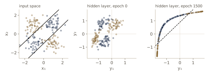
Before training, the least-squares discriminant in \(\mathbf{y}\)-space does no better than it would in \(\mathbf{x}\)-space: about chance. After training, the hidden representation is nearly linearly separable, and the linear discriminant and the network’s own output unit both reach a training error of about 0.09. The learned weights show how. Both hidden units have weight vectors close to the direction \((-1, 1)\), with biases of opposite sign, so their boundaries are two parallel lines, roughly \(x_2 - x_1 = 0.7\) and \(x_2 - x_1 = -0.55\). Between them lies a diagonal band that holds the two \(\omega_1\) blobs, and the output unit only has to ask whether a pattern is inside the band. That also explains why this network cannot reach the Bayes error of 0.044: the Bayes boundary is the pair of axes, \(x_1 x_2 = 0\), which a band between two parallel lines only approximates. The 2-4-1 network of the protocol experiment has enough hidden units to do better. The same thing happens in higher dimensions. In three-bit parity, for example, a 3-3-1 network moves the corners of the cube until a plane separates odd from even parity. And a problem that two hidden units cannot make separable may become separable with three, because the hidden space then has more room.
Representations at the hidden layer
The weights themselves are informative too. The input-to-hidden weights of unit \(j\), read as a pattern in input space, describe the input that excites the unit most (for inputs of fixed length the net activation \(\mathbf{w}_j^{t}\mathbf{x}\) is largest when \(\mathbf{x}\) points along \(\mathbf{w}_j\)). A hidden unit therefore acts somewhat like a matched filter, a detector for a particular input pattern (see the section on matched filters). When the inputs are pixels of small character images, displaying each hidden unit’s weights as an image often shows strokes or bar-like groupings that are useful for telling the characters apart.
Interpretation needs care. In large networks with many hidden units the learned weights often look unstructured, because the features we expect may not be the ones that matter, because important information lies in interactions between features that one unit’s weights do not show, or because superfluous weights spread each feature across many units. The hidden-to-output weights are harder still to read in terms of the inputs, since the hidden units have no natural order and each already encodes an abstract combination of inputs.
Backpropagation, Bayes theory, and probability
Multilayer networks can look like a bag of heuristics. The results of this section put them on the same footing as the Bayes classifier of module 02: trained on squared error with the right targets, a network’s outputs approximate the posterior probabilities.
Bayes discriminants and neural networks
Take a network with \(c\) outputs, let \(g_k(\mathbf{x}; \mathbf{w})\) be output \(k\), and train it with 0–1 targets: \(t_k = 1\) if the pattern belongs to \(\omega_k\) and \(t_k = 0\) otherwise. Consider the part of the training error that involves output \(k\), averaged over the \(n\) training patterns. As \(n \to \infty\) the average becomes an expectation over the joint distribution of \(\mathbf{x}\) and its class:
\[\lim_{n \to \infty} \frac{1}{n} \sum_{m=1}^{n} \left[ g_k(\mathbf{x}_m; \mathbf{w}) - t_{mk} \right]^2 = \mathcal{E}\left[ (g_k(\mathbf{x}; \mathbf{w}) - t_k)^2 \right] .\]Condition on \(\mathbf{x}\). Given \(\mathbf{x}\), the target \(t_k\) is a 0–1 random variable with mean \(\mathcal{E}[t_k \mid \mathbf{x}] = P(\omega_k \mid \mathbf{x})\) and variance \(P(\omega_k \mid \mathbf{x})(1 - P(\omega_k \mid \mathbf{x}))\). For any number \(g\), \(\mathcal{E}[(g - t)^2 \mid \mathbf{x}] = (g - \mathcal{E}[t \mid \mathbf{x}])^2 + \operatorname{Var}[t \mid \mathbf{x}]\), so
\[\begin{aligned} \mathcal{E}\left[ (g_k - t_k)^2 \right] &= \int \left[ g_k(\mathbf{x}; \mathbf{w}) - P(\omega_k \mid \mathbf{x}) \right]^2 p(\mathbf{x})\, d\mathbf{x} \\ &\quad + \int P(\omega_k \mid \mathbf{x}) \left[ 1 - P(\omega_k \mid \mathbf{x}) \right] p(\mathbf{x})\, d\mathbf{x} . \end{aligned}\]The second integral does not depend on the weights. Minimizing the squared error over \(\mathbf{w}\) is therefore the same as minimizing the first integral, the \(p(\mathbf{x})\)-weighted squared distance between the output and the posterior. Summing over \(k\) gives the same conclusion for the whole network.
Result. In the limit of infinite training data, a network trained on squared error with 0–1 targets gives the least-squares approximation to the posteriors: \(g_k(\mathbf{x}; \mathbf{w}) \approx P(\omega_k \mid \mathbf{x})\), with the approximation best where \(p(\mathbf{x})\) is large.
Two conditions hide in this statement. The network must be able to represent the posteriors, which requires enough hidden units; and the training set must be large, since with finite \(n\) we minimize a noisy estimate of the expectation. The argument does not depend on the targets being 0 and 1 in any essential way: with \(\pm 1\) targets the same algebra shows the outputs approximate \(2P(\omega_k \mid \mathbf{x}) - 1\).
We can test this on data where we know the posteriors. Our example has one feature and three classes with Gaussian class-conditional densities of different means, spreads, and priors. We train a 1-6-3 network with logistic-sigmoid outputs (whose range \((0, 1)\) matches 0–1 targets) on training sets of three sizes, and measure the root-mean-square distance between outputs and true posteriors, weighted by \(p(x)\). We also compute the irreducible part of the error, \(\tfrac12 \int \sum_k P(\omega_k \mid x)[1 - P(\omega_k \mid x)] p(x)\, dx\), which is the smallest per-pattern \(J\) any network can reach on average.
P_1d = np.array([0.35, 0.35, 0.30])                       # priors P(omega_k)
MU_1d, SD_1d = np.array([-1.5, 0.3, 1.8]), np.array([0.8, 0.5, 1.0])

def sample_1d(n, rng):
    y = rng.choice(3, n, p=P_1d)
    return (MU_1d[y] + SD_1d[y] * rng.standard_normal(n))[:, None], y

def posterior_1d(x, priors=P_1d):
    """True posteriors P(omega_k | x) by Bayes' formula, in log space."""
    lj = np.log(priors) + norm.logpdf(x[:, None], MU_1d, SD_1d)
    return np.exp(lj - logsumexp(lj, axis=1, keepdims=True))

x_grid = np.linspace(-4.5, 5.0, 400)
dx = x_grid[1] - x_grid[0]
p_x = np.sum(P_1d * norm.pdf(x_grid[:, None], MU_1d, SD_1d), axis=1)    # mixture density p(x)
P_true = posterior_1d(x_grid)
print(f"irreducible J/n = {0.5 * np.sum(p_x * np.sum(P_true * (1 - P_true), axis=1)) * dx:.4f}")

def weighted_rms(Z, P):
    return np.sqrt(np.sum(p_x[:, None] * (Z - P) ** 2) * dx)

nets_1d = {}
for n in [150, 600, 2400]:
    X1, y1 = sample_1d(n, np.random.default_rng(606))
    m1, s1 = X1.mean(), X1.std()                           # standardize the input
    W1, W2 = init_weights(1, 6, 3, np.random.default_rng(1))
    W1, W2, h = train_batch(W1, W2, (X1 - m1) / s1, np.eye(3)[y1], eta=0.5, epochs=3000,
                            alpha=0.9, out=LOGISTIC)
    Z = forward(W1, W2, (x_grid[:, None] - m1) / s1, out=LOGISTIC)[3]
    nets_1d[n] = (W1, W2, m1, s1)
    print(f"n = {n:4d}: training J/n = {h[-1, 0]:.4f}   rms(output - posterior) = {weighted_rms(Z, P_true):.4f}"
          f"   sum of outputs in [{Z.sum(1).min():.3f}, {Z.sum(1).max():.3f}]")
irreducible J/n = 0.1081
n =  150: training J/n = 0.1124   rms(output - posterior) = 0.0967   sum of outputs in [0.884, 1.015]
n =  600: training J/n = 0.1078   rms(output - posterior) = 0.0665   sum of outputs in [0.951, 1.036]
n = 2400: training J/n = 0.1091   rms(output - posterior) = 0.0371   sum of outputs in [0.974, 1.018]
The training error settles near the irreducible value, and the distance to the true posteriors shrinks steadily as the training set grows, by factors of about 0.7 and 0.55 for each fourfold increase in \(n\) (estimation noise alone would give 0.5, since it falls like \(1/\sqrt{n}\)). Notice also the last column: nothing forces the three outputs to sum to 1, and with finite data they do not, by up to about 12 percent for the smallest training set and 3 percent for the largest. A large departure from 1 in some region of input space is a useful warning that the network is not modeling the posteriors well there.
Outputs as probabilities
If we want the outputs to behave as probabilities, we can build that into the output layer. The softmax output unit uses an exponential activation and normalizes across the outputs for each pattern:
\[z_k = \frac{e^{net_k}}{\sum_{m=1}^{c} e^{net_m}} .\]The outputs are positive and sum to 1 by construction. Softmax is a smooth version of a winner-take-all rule, in which the largest output becomes 1 and the rest 0. It is also exactly the posterior of module 02 when the class-conditional densities of the hidden representation \(\mathbf{y}\) belong to a common exponential family (for instance, Gaussians with a shared covariance), which is one way to justify it.
Softmax outputs pair naturally with the cross-entropy criterion \(J = -\sum_m \sum_k t_{mk} \ln z_{mk}\), which we discuss again under criterion functions. The pairing makes the output sensitivity especially simple. For one pattern, \(\partial z_m / \partial net_k = z_m(\mathbb{1}[m = k] - z_k)\), so
\[\delta_k = -\frac{\partial J}{\partial net_k} = \sum_{m} \frac{t_m}{z_m} z_m (\mathbb{1}[m = k] - z_k) = t_k - z_k \sum_m t_m = t_k - z_k,\]using \(\sum_m t_m = 1\). That is the loss="ce" branch of backprop, and the gradient check above confirmed it. The same network trained this way on the 600-pattern set gives outputs that are exact probability vectors.
X1, y1 = sample_1d(600, np.random.default_rng(606))
m1, s1 = X1.mean(), X1.std()
W1, W2 = init_weights(1, 6, 3, np.random.default_rng(1))
W1_sm, W2_sm, h = train_batch(W1, W2, (X1 - m1) / s1, np.eye(3)[y1], eta=0.1, epochs=3000,
                              alpha=0.9, out=SOFTMAX, loss="ce")
Z_sm = forward(W1_sm, W2_sm, (x_grid[:, None] - m1) / s1, out=SOFTMAX)[3]
print(f"cross-entropy J/n = {h[-1, 0]:.4f}   rms(output - posterior) = {weighted_rms(Z_sm, P_true):.4f}"
      f"   sum of outputs in [{Z_sm.sum(1).min():.3f}, {Z_sm.sum(1).max():.3f}]")

# The priors change after training: rescale each output by P_new/P_old and renormalize.
P_new = np.array([0.6, 0.2, 0.2])
Z_adj = Z_sm * P_new / P_1d
Z_adj /= Z_adj.sum(axis=1, keepdims=True)
P_true_new = posterior_1d(x_grid, P_new)
print(f"new priors: rms without adjustment = {weighted_rms(Z_sm, P_true_new):.4f},"
      f"  with adjustment = {weighted_rms(Z_adj, P_true_new):.4f}")
cross-entropy J/n = 0.3558   rms(output - posterior) = 0.0595   sum of outputs in [1.000, 1.000]
new priors: rms without adjustment = 0.1659,  with adjustment = 0.0817
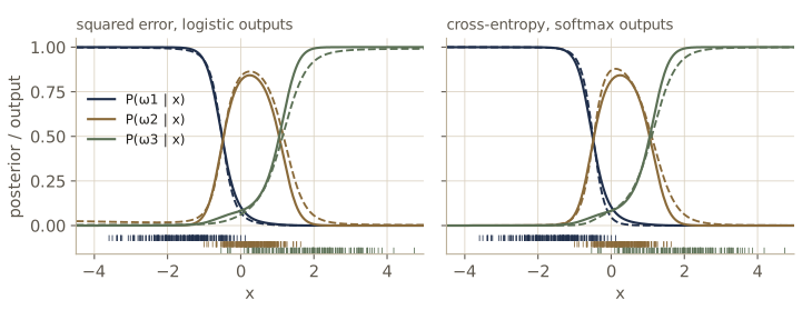
The softmax network matches the posteriors about as well as the squared-error network, and its outputs sum to 1 exactly. Because the outputs estimate posteriors, they carry the training priors with them. If the network is used where the priors are different, dividing each output by the old prior, multiplying by the new one, and renormalizing corrects for the change, as the second line shows (this is Bayes’ formula applied twice; it does not by itself guarantee the lowest error, since the network’s approximation errors are rescaled too). When the goal is only classification rather than probability estimates, other output codings, such as the \(\pm 1\) targets of the practical section below, often train faster.
Related statistical techniques
The network diagram is a useful picture, but mathematically a three-layer network is just the function \(g_k(\mathbf{x})\) written earlier, and several statistical methods have a similar form.
Projection pursuit regression models
\[z = \sum_{j=1}^{j_{\max}} w_j\, f_j(\mathbf{v}_j^{t}\mathbf{x} + v_{j0}) + w_0 .\]Each term projects \(\mathbf{x}\) onto a direction \(\mathbf{v}_j\) and passes the projection through its own nonlinear function \(f_j\); the terms are added linearly. The \(f_j\) are called ridge functions, because each is constant along the hyperplanes orthogonal to \(\mathbf{v}_j\) and so looks like a ridge over a two-dimensional input space. The \(\mathbf{v}_j\) play the role of input-to-hidden weights and the output is linear, but each \(f_j\) is a flexible function fitted to the data rather than a fixed sigmoid. The parameters are usually fitted one group at a time on squared error: the first direction and its ridge function, then the second, and so on, then the output weights, iterating to convergence.
A generalized additive model instead applies a nonlinear function to each input separately and passes the sum through an output nonlinearity,
\[z = f\left( \sum_{i=1}^{d} f_i(x_i) + w_0 \right),\]with the \(f_i\) fitted iteratively. Multivariate adaptive regression splines (MARS) build the output from a weighted sum of products of one-dimensional spline functions, added one at a time by a greedy search over which feature to split and where. All three methods predate the popularity of backpropagation. Networks largely replaced them in pattern recognition because gradient training of all weights at once scales better to many features and many patterns, because prior knowledge can be built into a network’s architecture and training (hints, weight sharing), and because networks admit the regularization and pruning methods of the last section.
Practical techniques for improving backpropagation
The derivations above are correct, but a naive implementation can train slowly, generalize poorly, or both. DHS collect a set of heuristics that experience has shown to help. Few of them come with proofs; most rest on simple arguments about scaling and conditioning, and each is easy to test.
Activation function
Backpropagation works with nearly any activation function whose value and derivative are continuous. Beyond that, a few properties are desirable:
- Nonlinearity. With linear hidden units, a three-layer network computes a linear function of \(\mathbf{x}\) and is no more powerful than a two-layer one (a product of linear maps is linear).
- Saturation. Bounded outputs keep activations and weights bounded, which helps when outputs represent probabilities or firing rates. (For regression with a wide range of outputs, a linear output unit is better.)
- Continuity and smoothness. The derivative must exist, which rules out the threshold units of the XOR construction for training. Piecewise-linear units can be made to work but add complications.
- Monotonicity. Not essential, but a nonmonotonic \(f\) with several maxima can add spurious minima to the error surface.
- Linearity near zero. Then a network with small weights implements a nearly linear model, a sensible starting point.
The sigmoids, such as the hyperbolic tangent and the logistic function, have all these properties, and their derivatives can be written in terms of the function itself, which saves computation. A layer of sigmoid units gives a distributed representation: a typical input activates many hidden units to some degree. Units that respond only in a small region of input space, such as the Gaussian units of the radial basis function networks below, give a local representation, as a nearest-neighbor classifier does. With few training patterns, distributed representations often generalize better, because each region of input space is influenced by more of the data. Polynomial classifiers, by contrast, use hidden “units” such as \(x_1^2\) or \(x_1 x_2\) whose values can become enormous, which saturating sigmoids avoid.
Parameters for the sigmoid
It helps to use an antisymmetric sigmoid, \(f(-net) = -f(net)\), centered on zero, rather than one that is always positive. Together with inputs centered at zero, it keeps the average signals into each layer near zero, which avoids large eigenvalues in the Hessian of the error and so speeds learning (the section on second-order methods makes this precise). A convenient family is
\[f(net) = a \tanh(b\, net) = a\, \frac{e^{b\, net} - e^{-b\, net}}{e^{b\, net} + e^{-b\, net}} .\]The overall scale and slope matter only relative to the learning rate, the input scale, and the targets. A common choice is \(a = 1.716\) and \(b = 2/3\). Then \(f(\pm 1) = \pm 1\), the function is nearly linear for \(-1 < net < 1\), and it saturates at \(\pm 1.716\). Its derivative is \(f'(net) = ab\,[1 - \tanh^2(b\, net)] = (b/a)(a^2 - f^2)\), a function of \(f\) itself.
f, df = TANH.f, TANH.df
net = np.linspace(-4, 4, 80001)
d2f = np.gradient(df(net), net)                           # numerical second derivative
print(f"f(1) = {f(1.0):.4f}, f(-1) = {f(-1.0):.4f}, saturation = +-{A_TANH}")
print(f"f'(0) = {df(0.0):.4f};  f'(1)/f'(0) = {df(1.0) / df(0.0):.3f}")
print(f"f'' is most negative at net = {net[np.argmin(d2f)]:.3f}")
print("f' = (b/a)(a^2 - f^2):", np.allclose(df(net), B_TANH / A_TANH * (A_TANH**2 - f(net)**2)))
f(1) = 1.0001, f(-1) = -1.0001, saturation = +-1.716
f'(0) = 1.1440;  f'(1)/f'(0) = 0.660
f'' is most negative at net = 0.988
f' = (b/a)(a^2 - f^2): True
The slope at the origin is about 1.14 and still about two-thirds of that at \(net = \pm 1\), so the unit is close to linear over that range, and the curvature of \(f\) peaks near \(net = \pm 1\), where the nonlinearity starts to bite. This is the TANH activation we have been using.
Scaling the input
Suppose one feature is a mass in grams, with values in the thousands, and another a length in meters, with values below one. The net activation of every hidden unit is then dominated by the mass, the error depends almost only on the weights from the mass input, and gradient descent adjusts those weights far more than the others. Measuring in kilograms and millimeters would reverse the preference, although the information is the same. The remedy is to standardize the inputs: shift each feature to mean zero and scale it to unit variance over the training set, once, before training, and apply the same transformation to every later pattern. (This resembles the whitening transformation of module 02, but acts on each feature separately.) Standardization needs the whole training set, so it fits stochastic and batch protocols but not a strict on-line one.
We test this on the noisy XOR with its two features expressed in awkward units: the first multiplied by 200 and shifted by 1000, the second multiplied by 0.05 and shifted by 0.3. For the raw features we try a range of learning rates and keep the best.
def standardize(X_train, *others):
    m, s = X_train.mean(axis=0), X_train.std(axis=0)
    return [(Z - m) / s for Z in (X_train,) + others]

scale_units, shift_units = np.array([200.0, 0.05]), np.array([1000.0, 0.3])
X_raw, X_rawt = X_nx * scale_units + shift_units, X_nxt * scale_units + shift_units
W1, W2 = init_weights(2, 4, 1, np.random.default_rng(4))
for eta in [1e-4, 1e-2, 1.0]:
    A, B, h = train_batch(W1, W2, X_raw, T_nx, eta=eta, epochs=500, alpha=0.9)
    err = np.mean(classify(A, B, X_rawt) != y_nxt)
    print(f"raw units, eta = {eta:g}:  J/n = {h[-1, 0]:.3f}  test error = {err:.3f}")
X_std, X_stdt = standardize(X_raw, X_rawt)
A, B, h = train_batch(W1, W2, X_std, T_nx, eta=0.5, epochs=500, alpha=0.9)
err = np.mean(classify(A, B, X_stdt) != y_nxt)
print(f"standardized, eta = 0.5:  J/n = {h[-1, 0]:.3f}  test error = {err:.3f}")
raw units, eta = 0.0001:  J/n = 1.701  test error = 0.496
raw units, eta = 0.01:  J/n = 0.499  test error = 0.504
raw units, eta = 1:  J/n = 0.499  test error = 0.504
standardized, eta = 0.5:  J/n = 0.068  test error = 0.048
With raw units no learning rate works: the hidden units are saturated from the first pattern (their net activations are in the hundreds), so their derivatives vanish, and the tiny second feature has no influence anyway. After standardization the same network with the same starting weights learns the problem in a few hundred epochs.
Target values
With 1-of-\(c\) coding and the scaled tanh at the outputs, it is tempting to set the targets to the saturation values \(\pm 1.716\). That is a mistake: the outputs can reach those values only as \(net_k \to \pm\infty\), so there is always some error left, and training keeps pushing the weights toward infinity. The usual choice is \(+1\) for the target class and \(-1\) for the others, for example \(\mathbf{t} = (-1, -1, +1, -1)^{t}\) for a pattern from \(\omega_3\) of four classes. These targets are reachable with finite weights. The price is that such outputs are not posteriors (they approximate \(2P(\omega_k \mid \mathbf{x}) - 1\)), which is fine when we only need the class.
for t_level in [1.0, A_TANH]:
    W1, W2 = init_weights(2, 2, 1, np.random.default_rng(0))
    norms = []
    for epochs in [500, 2000, 8000]:
        A, B, _ = train_batch(W1, W2, X_xor, t_level * t_xor[:, None], eta=0.1, epochs=epochs, alpha=0.9)
        norms.append(np.sqrt(np.sum(A**2) + np.sum(B**2)))
    print(f"targets +-{t_level:.3f}: weight norm after 500, 2000, 8000 epochs =", np.round(norms, 2))
targets +-1.000: weight norm after 500, 2000, 8000 epochs = [3.89 3.9  3.9 ]
targets +-1.716: weight norm after 500, 2000, 8000 epochs = [5.91 6.77 7.47]
With \(\pm 1\) targets the weights settle; with \(\pm 1.716\) they keep growing with training time.
Training with noise
With a small training set, we can enlarge it with surrogate patterns: copies of the real patterns with random noise added, keeping their labels. Without specific knowledge of the problem, a natural choice is spherical Gaussian noise; for standardized inputs its variance should be well below 1, say 0.1. Training with noise works with most classifiers, but it does little for very local ones such as nearest-neighbor rules. The experiment uses 40 noisy-XOR training patterns and an oversized network, with and without four noisy copies of each pattern, for three different training sets.
for data_seed in [31, 32, 33]:
    Xs_, ys_ = noisy_xor(40, np.random.default_rng(data_seed), 0.7)
    noise_rng = np.random.default_rng(data_seed + 100)
    X_aug = np.vstack([Xs_] + [Xs_ + np.sqrt(0.1) * noise_rng.standard_normal(Xs_.shape) for _ in range(4)])
    y_aug = np.tile(ys_, 5)
    errs = []
    for Xa, ya in [(Xs_, ys_), (X_aug, y_aug)]:
        W1, W2 = init_weights(2, 10, 1, np.random.default_rng(7))
        A, B, _ = train_batch(W1, W2, Xa, pm_targets(ya), eta=0.2, epochs=2000, alpha=0.9)
        errs.append(np.mean(classify(A, B, X_te) != y_te))
    print(f"training set {data_seed}: test error {errs[0]:.3f} without noise, {errs[1]:.3f} with noise")
print(f"Bayes error for s = 0.7: {xor_bayes_error(0.7):.3f}")
training set 31: test error 0.203 without noise, 0.191 with noise
training set 32: test error 0.217 without noise, 0.169 with noise
training set 33: test error 0.171 without noise, 0.164 with noise
Bayes error for s = 0.7: 0.141
The noisy copies act as a smoothness prior: they tell the network that nearby inputs should get the same label, which discourages the small wiggles in the boundary that fit individual patterns. The effect varies from one training set to another but is consistently in the right direction here.
Manufacturing data
If we know how patterns vary, we can do better than uncorrelated noise and manufacture training data that encodes that knowledge. In character recognition, rotating, shifting, scaling, or thickening the strokes of a training image gives new images of the same character, and if we know the likely range of each variation we can match it. This amounts to building prior information into the training set; compared with writing that prior into a likelihood, it only needs a way to generate transformed patterns. Like training with noise, it works with many classifiers; the costs are memory and training time for the enlarged set. The ML notes treat the same idea together with its alternatives, tangent propagation and invariant architectures, in Intro to ML, module 05.
Number of hidden units
The numbers of input and output units are fixed by the dimension of the features and the number of classes; the number of hidden units \(n_H\) is ours to choose, and it sets the expressive power of the network. Well-separated classes need few hidden units; classes with complicated, interleaved densities need more. Too few, and the network cannot fit even the training data; too many, and it fits the training data’s quirks and generalizes poorly. The cell trains networks of different sizes on 200 noisy-XOR patterns with \(s = 0.7\).
X_h, y_h = noisy_xor(200, np.random.default_rng(21), 0.7)
print(" n_H  weights   train J/n   train error   test error")
for n_H_try in [1, 2, 3, 4, 6, 10, 20]:
    W1, W2 = init_weights(2, n_H_try, 1, np.random.default_rng(8))
    A, B, h = train_batch(W1, W2, X_h, pm_targets(y_h), eta=0.2, epochs=3000, alpha=0.9)
    print(f"{n_H_try:4d}  {A.size + B.size:6d}   {h[-1, 0]:9.3f}   {np.mean(classify(A, B, X_h) != y_h):10.3f}"
          f"   {np.mean(classify(A, B, X_te) != y_te):9.3f}")
 n_H  weights   train J/n   train error   test error
   1       5       0.413        0.335       0.360
   2       9       0.306        0.220       0.232
   3      13       0.191        0.115       0.168
   4      17       0.181        0.115       0.179
   6      25       0.177        0.120       0.178
  10      41       0.177        0.115       0.180
  20      81       0.160        0.110       0.173
One hidden unit cannot represent XOR, and its test error is far from the others. Two hidden units can only make a band, as in the feature-mapping example, and are still clearly worse. From three hidden units on, the training criterion keeps falling slowly as the network grows, but the test error stays flat near 0.17–0.18: more hidden units buy nothing here. (They do not hurt much either, because batch training from small weights for a fixed number of epochs limits how far the extra weights move; with only 60 training patterns, the learning-curve experiment showed a large network overfitting clearly.) A rule of thumb from DHS is to choose \(n_H\) so that the total number of weights is roughly \(n/10\); here that is about 20 weights, or four to five hidden units, consistent with what we see. The rule is only a starting point, and many successful networks are larger. A more principled approach is to start with a generous network and cut back its complexity with weight decay or pruning, as in the sections below and in module 09.
Initializing weights
We cannot start at zero, as the backpropagation rules showed. We want uniform learning, meaning all weights reach their final values at about the same time; if some weights (or some classes) are learned much earlier than others, the network can end up with an error rate well above what it could achieve. Since standardized inputs are positive and negative equally often, we draw the weights symmetrically from a uniform distribution on \((-\tilde{w}, \tilde{w})\) and choose \(\tilde{w}\) so that each hidden unit starts in its linear range: small enough not to saturate, large enough not to be trivially linear.
A hidden unit with \(d\) standardized inputs and independent uniform weights has net activation with variance \(d\, \tilde{w}^2 / 3\), since each term \(w_{ji} x_i\) has variance \(\tilde{w}^2/3\). Choosing \(\tilde{w} = 1/\sqrt{d}\) gives a standard deviation of \(1/\sqrt{3} \approx 0.58\), comfortably inside \(-1 < net_j < 1\). The same argument for the output units gives \(\tilde{w} = 1/\sqrt{n_H}\) for the hidden-to-output weights. These are the ranges in init_weights.
d_init, n_init = 10, 5000
X_init = rng.standard_normal((n_init, d_init))                  # standardized inputs
W1, W2 = init_weights(d_init, 20, 3, np.random.default_rng(9))
net_h, Y, net_o, _ = forward(W1, W2, X_init)
for name, net in [("hidden", net_h), ("output", net_o)]:
    print(f"{name} net activations: std = {net.std():.3f}, fraction in (-1, 1) = {np.mean(np.abs(net) < 1):.3f}")
hidden net activations: std = 0.592, fraction in (-1, 1) = 0.907
output net activations: std = 0.354, fraction in (-1, 1) = 0.992
Both layers start where we want them, and the XOR experiment above showed the cost of ignoring this: three times larger initial weights left a quarter of the runs stuck.
Learning rates
For a small enough learning rate, gradient descent reaches the same minimum whatever \(\eta\) is; only the speed changes. In practice we rarely train to a minimum, so \(\eta\) can affect the final network as well. A principled choice comes from a quadratic model. Near a minimum \(w^*\) of a one-dimensional criterion, \(J(w) \approx J(w^*) + \tfrac12 J''\, (w - w^*)^2\), so \(J'(w) = J''(w - w^*)\), and one step of size \(\eta\) gives
\[w - w^* \;\leftarrow\; (1 - \eta J'')(w - w^*) .\]The step lands exactly on the minimum when
\[\eta_{\text{opt}} = \left( \frac{\partial^2 J}{\partial w^2} \right)^{-1} .\]For \(\eta < \eta_{\text{opt}}\) the iterates approach \(w^*\) monotonically but slowly; for \(\eta_{\text{opt}} < \eta < 2\eta_{\text{opt}}\) they overshoot and oscillate but still converge; for \(\eta > 2\eta_{\text{opt}}\) the factor \(\lvert 1 - \eta J'' \rvert\) exceeds 1 and they diverge.
J2, w_star = 4.0, 1.0                                       # J(w) = 1/2 J2 (w - w*)^2
eta_opt = 1.0 / J2
for ratio in [0.5, 1.0, 1.5, 2.1]:
    w, path = -1.0, []
    for step in range(5):
        w = w - ratio * eta_opt * J2 * (w - w_star)          # w <- w - eta dJ/dw
        path.append(w)
    print(f"eta = {ratio:.1f} eta_opt:  w =", np.round(path, 3))
eta = 0.5 eta_opt:  w = [0.    0.5   0.75  0.875 0.938]
eta = 1.0 eta_opt:  w = [1. 1. 1. 1. 1.]
eta = 1.5 eta_opt:  w = [2.    0.5   1.25  0.875 1.062]
eta = 2.1 eta_opt:  w = [ 3.2   -1.42   3.662 -1.928  4.221]
In several dimensions the curvature differs from direction to direction, and the largest curvature limits \(\eta\) while the smallest sets the speed. This is why DHS suggest, ideally, a separate learning rate per weight based on its own second derivative, and it is the motivation for the second-order methods below. For sigmoid networks with standardized inputs and the parameters above, \(\eta \approx 0.1\) is a reasonable first try; lower it if the error diverges and raise it if learning crawls.
Momentum
Error surfaces often contain plateaus where the gradient is tiny, and long narrow valleys where the gradient points mostly across the valley rather than along it. Momentum adds a fraction of the previous weight change to the current one, so that the weights keep moving in directions that are consistently downhill and changes that alternate in sign cancel. With \(\Delta \mathbf{w}(m) = \mathbf{w}(m) - \mathbf{w}(m-1)\) and \(\Delta \mathbf{w}_{bp}(m)\) the change backpropagation alone would make, DHS write
\[\mathbf{w}(m+1) = \mathbf{w}(m) + (1 - \alpha)\, \Delta \mathbf{w}_{bp}(m) + \alpha\, \Delta \mathbf{w}(m-1) .\]For \(\alpha = 0\) this is plain backpropagation; for \(\alpha = 1\) the gradient is ignored and the weights move at constant velocity. Stability requires \(0 \le \alpha < 1\), and \(\alpha \approx 0.9\) is typical. The update is a first-order recursive low-pass filter applied to the sequence of weight changes, which is why it averages out the randomness of stochastic updates. This is the form in train_batch. (The ML notes and most software use the “heavy ball” form without the factor \(1 - \alpha\); the two are the same method with learning rates differing by that factor.)
With the factor \(1 - \alpha\), the steady-state step on a constant gradient is still \(\eta\) times the gradient, so momentum does not speed up travel along a straight slope by itself. Its gain is that it damps oscillation, which lets us use a much larger learning rate. The cell measures this on an ill-conditioned quadratic, \(J(\mathbf{w}) = \tfrac12 \mathbf{w}^{t}\mathbf{H}\mathbf{w}\) with Hessian eigenvalues 5 and 0.2, choosing the best learning rate for each method from a grid.
theta = np.deg2rad(30)
R = np.array([[np.cos(theta), -np.sin(theta)], [np.sin(theta), np.cos(theta)]])
H_q = R @ np.diag([5.0, 0.2]) @ R.T                           # condition number 25
w_start = np.array([-2.5, 2.0])

def descend(eta, alpha, w=w_start, iters=500, tol=1e-8):
    """Gradient descent with DHS momentum on J = 1/2 w^t H w; returns the path and iterations to tol."""
    b, path = np.zeros(2), [w.copy()]
    for m in range(iters):
        b = -eta * (1 - alpha) * (H_q @ w) + alpha * b
        w = w + b
        path.append(w.copy())
        J = 0.5 * w @ H_q @ w
        if J < tol:
            return np.array(path), m + 1
        if J > 1e6:                                        # diverged
            break
    return np.array(path), iters

etas = np.linspace(0.02, 4.0, 200)
for alpha in [0.0, 0.5, 0.8, 0.9]:
    its = [descend(eta, alpha)[1] for eta in etas]
    best = int(np.argmin(its))
    print(f"alpha = {alpha:.1f}: best eta = {etas[best]:.2f}, iterations to J < 1e-8 = {its[best]}")
alpha = 0.0: best eta = 0.38, iterations to J < 1e-8 = 116
alpha = 0.5: best eta = 0.96, iterations to J < 1e-8 = 28
alpha = 0.8: best eta = 2.68, iterations to J < 1e-8 = 53
alpha = 0.9: best eta = 0.68, iterations to J < 1e-8 = 106
Plain gradient descent is limited by the steep direction: any \(\eta\) above \(2/5\) diverges, and at the best allowed \(\eta\) progress along the shallow direction is slow. With \(\alpha = 0.5\) the best learning rate is more than twice as large and the number of iterations drops about fourfold. More momentum is not better: at \(\alpha = 0.9\) the weights overshoot and spiral in slowly. The theory of the heavy-ball method explains both observations. With the best settings, the convergence factor per iteration improves from \((\kappa - 1)/(\kappa + 1)\) to \((\sqrt{\kappa} - 1)/(\sqrt{\kappa} + 1)\), where \(\kappa\) is the condition number of \(\mathbf{H}\), and the best momentum is \(\alpha = ((\sqrt{\kappa} - 1)/(\sqrt{\kappa} + 1))^2 \approx 0.44\) for our \(\kappa = 25\). The left panel of the convergence figure in the section on conjugate gradients shows the two paths.
Weight decay
A simple way to discourage overfitting in a network with too many weights is to prefer small weights. Weight decay shrinks every weight a little after each update,
\[w^{\text{new}} = w^{\text{old}}(1 - \epsilon), \qquad 0 < \epsilon < 1 .\]Weights that the error does not need decay toward zero and may eventually be removed; weights that reduce the error settle where the error’s pull balances the decay. Small weights keep the sigmoids in their linear range, so weight decay pushes the network toward simpler, more nearly linear functions. It is not guaranteed to help, but it usually does, and it costs one line of code (the decay argument of train_batch).
Decay is gradient descent on a modified criterion. A gradient step followed by decay gives
\[(\mathbf{w} - \eta \nabla J)(1 - \epsilon) = \mathbf{w} - \eta \left[ \nabla J + \frac{\epsilon}{\eta} \mathbf{w} \right] + \epsilon\eta \nabla J,\]and the last term is of second order in the small quantities \(\epsilon\) and \(\eta\). To first order, then, decay is gradient descent on the effective criterion
\[J_{ef}(\mathbf{w}) = J(\mathbf{w}) + \frac{\epsilon}{2\eta}\, \mathbf{w}^{t}\mathbf{w},\]whose second term is a regularization term that penalizes large weights. (DHS write the constant differently; the constant only rescales \(\epsilon\), which is tuned in practice.) The quadratic penalty charges most for a single large weight. A variant divides the penalty for each weight by a function of its size relative to \(\mathbf{w}^{t}\mathbf{w}\), which spreads the penalty across the network and is more willing to leave some weights large while eliminating others.
We return to the overfitting experiment of the learning curves, 60 patterns and 10 hidden units, and train to the end with several decay rates.
print("  epsilon   train J/n   test error   weight norm")
for eps in [0.0, 3e-4, 1e-3, 3e-3, 1e-2, 3e-2]:
    A, B, h = train_batch(W1_lc0, W2_lc0, X_tr, pm_targets(y_tr), eta=0.2, epochs=3000, alpha=0.9, decay=eps)
    print(f"  {eps:7.0e}   {h[-1, 0]:9.3f}   {np.mean(classify(A, B, X_te) != y_te):10.3f}"
          f"   {np.sqrt(np.sum(A**2) + np.sum(B**2)):11.2f}")
  epsilon   train J/n   test error   weight norm
    0e+00       0.069        0.187          5.84
    3e-04       0.074        0.181          4.74
    1e-03       0.081        0.176          4.18
    3e-03       0.102        0.171          3.61
    1e-02       0.180        0.186          2.80
    3e-02       0.459        0.461          0.43
As \(\epsilon\) grows, the weights shrink, the training error rises, and the test error first improves, by about 0.015 at \(\epsilon = 0.003\). Too much decay (\(\epsilon = 0.03\)) leaves weights too small to model XOR at all, and the network falls back to chance. The best \(\epsilon\) must be found by validation, like the number of hidden units.
Hints
When training data are scarce, we can sometimes add information through hints: extra output units trained on an ancillary task related to the real one. For a network that classifies phonemes, we might add two outputs that indicate whether the sound is a vowel or a consonant, and extend each target vector with the corresponding values. The hint outputs share the hidden layer with the class outputs, so the hidden units are pushed toward features useful for both tasks, and features that separate vowels from consonants are likely to help separate individual phonemes too. After training the hint units and their weights are discarded. Alternatively, one can train on the hint task first to develop good hidden units. Hints are easier to add to a network than to most other classifiers, nearest-neighbor rules or MARS for example.
On-line, stochastic, or batch training?
On-line training is for situations where storing the data is impractical: very large or unending streams, or tight memory. Most classification problems are handled with batch or stochastic training, and of the two, stochastic training is usually faster. The reason is redundancy. Imagine a training set of 200 patterns made of 10 copies each of 20 distinct patterns. Batch training computes the average gradient, which is exactly the average gradient over the 20 distinct patterns; the copies add work but no information. Stochastic training makes 200 updates per epoch, each informative.
X20, y20 = noisy_xor(20, np.random.default_rng(41))
X_dup, y_dup = np.tile(X20, (10, 1)), np.tile(y20, 10)          # 10 copies of 20 patterns
W1, W2 = init_weights(2, 4, 1, np.random.default_rng(4))
_, _, h_bat = train_batch(W1, W2, X_dup, pm_targets(y_dup), eta=0.5, epochs=31)
_, _, h_sto = train_stochastic(W1, W2, X_dup, pm_targets(y_dup), eta=0.02, epochs=30,
                               rng=np.random.default_rng(42))
for r in [1, 3, 10, 30]:
    print(f"after {r:2d} epochs   J/n batch = {h_bat[r, 0]:.4f}   stochastic = {h_sto[r - 1]:.4f}")
after  1 epochs   J/n batch = 0.4548   stochastic = 0.3914
after  3 epochs   J/n batch = 0.4185   stochastic = 0.3573
after 10 epochs   J/n batch = 0.3800   stochastic = 0.0356
after 30 epochs   J/n batch = 0.1538   stochastic = 0.0198
Real data sets rarely contain exact duplicates, but they are usually redundant in the same sense, so the argument carries over. Batch training has its own advantage: it allows the second-order methods of the next section, which need an accurate gradient of the full criterion.
Stopped training
A network with many weights, trained too long, fits a boundary tuned to its training patterns. DHS call this overfitting rather than “overtraining” because the problem is the complexity of the fitted function, not the training itself; a two-layer network can be trained forever without harm, because its boundary is always a hyperplane. Starting from small weights, a multilayer network begins as an almost linear model and becomes more nonlinear as its weights grow, so halting early limits its complexity. The practical rule is stopped training: stop at the minimum of the validation error. Setting a threshold on the training error in advance is much harder.
W1_stop, W2_stop, _ = train_batch(W1_lc0, W2_lc0, X_tr, pm_targets(y_tr), eta=0.2, epochs=r_stop, alpha=0.9)
for name, (A, B) in [(f"stopped at epoch {r_stop}", (W1_stop, W2_stop)),
                     ("trained 3000 epochs", (W1_lc, W2_lc))]:
    print(f"{name:22s} test error = {np.mean(classify(A, B, X_te) != y_te):.3f}"
          f"   weight norm = {np.sqrt(np.sum(A**2) + np.sum(B**2)):.2f}")
print(f"Bayes error = {xor_bayes_error(s_lc):.3f}")
stopped at epoch 136   test error = 0.174   weight norm = 3.92
trained 3000 epochs    test error = 0.187   weight norm = 5.84
Bayes error = 0.141
The stopped network is better on the test set and has much smaller weights. That is no coincidence: stopping early from small initial weights behaves much like weight decay, since both keep the weights near the origin (the ML notes show that for a quadratic error the two are closely related).
Number of hidden layers
Backpropagation works for any number of layers of differentiable units. For a network with layers \(\ell = 1, \dots, L\), the sensitivities follow the same recursion we derived for one hidden layer,
\[\delta_j^{(\ell)} = f'(net_j^{(\ell)}) \sum_k w_{kj}^{(\ell+1)} \delta_k^{(\ell+1)}, \qquad \Delta w_{ji}^{(\ell)} = \eta\, \delta_j^{(\ell)}\, y_i^{(\ell-1)},\]started at the output layer with \(\delta_k = (t_k - z_k) f'(net_k)\) and with \(y^{(0)} = \mathbf{x}\). Since one hidden layer already suffices to approximate any function, the case for more needs a reason from the problem. A common one is invariance: in character recognition, if each layer handles a small shift of the image, a stack of layers can handle a larger one, which is easier than learning the whole invariance in a single layer. Some functions also need far fewer units with two hidden layers than with one. On the other hand, DHS report that networks with several hidden layers are more prone to poor local minima in practice. Their advice is to start with one hidden layer and try two if needed.
Criterion function
Squared error is the most common criterion: it is simple, nonnegative, and makes several theorems easy to prove. The main alternative is the cross-entropy, which compares target and output as probability distributions,
\[J_{ce}(\mathbf{w}) = \sum_{m=1}^{n} \sum_{k=1}^{c} t_{mk} \ln \frac{t_{mk}}{z_{mk}} ,\]where targets and outputs must lie between 0 and 1. With 0–1 targets the \(t \ln t\) terms vanish (taking \(0 \ln 0 = 0\)) and this is the \(-\sum t_{mk} \ln z_{mk}\) we used with softmax outputs. Cross-entropy is the negative log-likelihood of the targets when the outputs are class probabilities, which is why it pairs with softmax so well; the ML notes derive both criteria from likelihoods.
A third choice is the Minkowski error \(\sum_m \sum_k \lvert z_{mk} - t_{mk} \rvert^R\). With \(1 \le R < 2\), patterns with large errors (often far from the decision boundary, in the tails of the distributions) count less than under squared error, so smaller \(R\) gives a more local classifier. Its backpropagation rule differs only in the output sensitivity, which becomes \(\delta_k = R\, \lvert t_k - z_k \rvert^{R-1} \operatorname{sgn}(t_k - z_k) f'(net_k)\).
The heuristics of this section can be combined, and they sometimes interact in unexpected ways. All of them have been useful on real problems, and experience with each is worth having.
Second-order methods
The learning-rate analysis already used second derivatives. Using them more fully gives faster training methods, and, in the last section, a principled way to remove weights.
The Hessian matrix
For a network with a single output and \(J(\mathbf{w}) = \frac{1}{2n} \sum_{m=1}^{n} (t_m - z_m)^2\), differentiating twice gives
\[\frac{\partial^2 J}{\partial w_p \partial w_q} = \frac{1}{n} \sum_{m=1}^{n} \left[ \frac{\partial z_m}{\partial w_p} \frac{\partial z_m}{\partial w_q} - (t_m - z_m) \frac{\partial^2 z_m}{\partial w_p \partial w_q} \right],\]where \(w_p\) and \(w_q\) are any two weights, in either layer. The second term is multiplied by the residuals \(t_m - z_m\), which are small for a network that fits well and tend to cancel across patterns, so it is often dropped. What remains is the outer-product approximation
\[\mathbf{H} \approx \frac{1}{n} \sum_{m=1}^{n} \mathbf{X}^{[m]} \mathbf{X}^{[m]t}, \qquad \mathbf{X} = \frac{\partial z}{\partial \mathbf{w}},\]which needs only first derivatives and is positive semidefinite by construction. (It is also called the Gauss–Newton or Levenberg–Marquardt approximation.) The derivatives come from the same chain rule as backpropagation: for hidden-to-output weights \(\partial z / \partial w_{kj} = f'(net_k)\, y_j\), and for input-to-hidden weights \(\partial z / \partial w_{ji} = f'(net_k)\, w_{kj}\, f'(net_j)\, x_i\).
To have a network where some weights are clearly unnecessary (useful again for pruning), we make a new two-feature data set in which only \(x_1\) matters: \(\omega_1\) is the band \(\lvert x_1 \rvert < 0.8\), with 5% of labels flipped, and \(x_2\) is pure noise. A 2-3-1 network is trained with a little weight decay. We then compare the outer-product approximation with the full Hessian, computed by central differences of the backpropagation gradient.
def output_jacobian(W1, W2, X, hid=TANH, out=TANH):
    """Rows dz/dw for a single-output network, in the order of pack(W1, W2)."""
    net_h, Y, net_o, _ = forward(W1, W2, X, hid, out)
    fo = out.df(net_o)                                     # f'(net_k), shape (n, 1)
    X_v = fo * augment(Y)                                  # dz/dw_kj = f'(net_k) y_j
    back = fo * W2[:, 1:] * hid.df(net_h)                  # f'(net_k) w_kj f'(net_j)
    X_u = back[:, :, None] * augment(X)[:, None, :]        # dz/dw_ji = f'(net_k) w_kj f'(net_j) x_i
    return np.column_stack([X_u.reshape(len(X), -1), X_v])

def hessian_fd(grad_of_w, w, h=1e-5):
    """Full Hessian by central differences of an analytic gradient."""
    H = np.zeros((len(w), len(w)))
    for q in range(len(w)):
        e = np.zeros_like(w); e[q] = h
        H[:, q] = (grad_of_w(w + e) - grad_of_w(w - e)) / (2 * h)
    return 0.5 * (H + H.T)

X_band = np.random.default_rng(51).standard_normal((200, 2))
y_band = np.where((np.abs(X_band[:, 0]) < 0.8) ^ (np.random.default_rng(52).random(200) < 0.05), 0, 1)
T_band = pm_targets(y_band)
W1, W2 = init_weights(2, 3, 1, np.random.default_rng(1))
W1_bd, W2_bd, h = train_batch(W1, W2, X_band, T_band, eta=0.2, epochs=3000, alpha=0.9, decay=1e-4)
w_bd = pack(W1_bd, W2_bd)
grad_J = lambda w: pack(*backprop(*unpack(w, 2, 3, 1), X_band, T_band)[1:]) / 200
print(f"J/n = {h[-1, 0]:.4f}, training error = {np.mean(classify(W1_bd, W2_bd, X_band) != y_band):.3f}")

Jac = output_jacobian(W1_bd, W2_bd, X_band)
j_num = numerical_gradient(lambda w: forward(*unpack(w, 2, 3, 1), X_band[:1])[3][0, 0], w_bd)
print(f"Jacobian check, pattern 0: max difference = {np.max(np.abs(Jac[0] - j_num)):.1e}")
H_full = hessian_fd(grad_J, w_bd)
H_op = Jac.T @ Jac / 200
rel = np.linalg.norm(H_full - H_op) / np.linalg.norm(H_full)
print(f"relative difference ||H - H_op|| / ||H|| = {rel:.3f}")
print("eigenvalues of H:   ", np.linalg.eigvalsh(H_full)[[0, 1, 2, -1]].round(4), "(smallest three, largest)")
print("eigenvalues of H_op:", np.linalg.eigvalsh(H_op)[[0, 1, 2, -1]].round(4))
J/n = 0.1575, training error = 0.070
Jacobian check, pattern 0: max difference = 1.4e-10
relative difference ||H - H_op|| / ||H|| = 0.046
eigenvalues of H:    [-0.0003  0.0007  0.0019  4.6746] (smallest three, largest)
eigenvalues of H_op: [0.0005 0.0006 0.0011 4.6019]
The approximation captures the large-scale structure of the Hessian: the largest eigenvalues agree closely and the overall difference is modest. It differs mostly in the smallest eigenvalues, where the full Hessian can even be slightly negative (the network is not at an exact minimum, and the residual term matters in flat directions) while the outer product never is. The spread of the eigenvalues, several orders of magnitude, is the ill-conditioning that makes plain gradient descent slow.
Newton’s method
Expand the change in the criterion to second order in a weight change \(\Delta\mathbf{w}\):
\[\Delta J = J(\mathbf{w} + \Delta\mathbf{w}) - J(\mathbf{w}) \approx \nabla J^{t} \Delta\mathbf{w} + \frac12 \Delta\mathbf{w}^{t} \mathbf{H}\, \Delta\mathbf{w} .\]Setting the derivative with respect to \(\Delta\mathbf{w}\) to zero gives \(\nabla J + \mathbf{H}\Delta\mathbf{w} = \mathbf{0}\), so the best step under the quadratic model is
\[\Delta\mathbf{w} = -\mathbf{H}^{-1} \nabla J, \qquad \mathbf{w}(m+1) = \mathbf{w}(m) - \mathbf{H}^{-1}(m)\, \nabla J(\mathbf{w}(m)) .\]This is Newton’s method, the multidimensional form of \(\eta_{\text{opt}} = 1/J''\). On a quadratic it reaches the minimum in one step. On a network it has two drawbacks. The Hessian has \(N^2\) entries for \(N\) weights and solving with it costs \(O(N^3)\) operations, which is prohibitive for large networks. More seriously, away from a well-behaved minimum the Hessian need not be positive definite, and then the Newton step can head uphill or toward a saddle point; a nearly singular Hessian makes the step enormous.
A common repair, not in DHS but worth knowing, combines the outer-product approximation with a damping term: \(\Delta\mathbf{w} = -(\mathbf{H}_{op} + \mu\mathbf{I})^{-1}\nabla J\). The matrix is always positive definite, so the step always points downhill. For large \(\mu\) it is a short gradient-descent step with \(\eta = 1/\mu\); for small \(\mu\) it approaches a Newton step with the approximate Hessian. This is the Levenberg–Marquardt method (in its full form it adjusts \(\mu\) at every step). The cell compares it with plain Newton on the band network.
g0 = H_q @ w_start
print("quadratic: one Newton step from", w_start, "->", w_start - np.linalg.solve(H_q, g0))

J_band = lambda w: backprop(*unpack(w, 2, 3, 1), X_band, T_band)[0] / 200
w_rand = pack(*init_weights(2, 3, 1, np.random.default_rng(1)))
for label, w_init in [("trained weights", w_bd), ("random weights", w_rand)]:
    w_n, w_lm = w_init.copy(), w_init.copy()
    J_n, J_lm = [J_band(w_n)], [J_band(w_lm)]
    for it in range(6):
        w_n = w_n - np.linalg.solve(hessian_fd(grad_J, w_n), grad_J(w_n))       # Newton, full Hessian
        Jac = output_jacobian(*unpack(w_lm, 2, 3, 1), X_band)
        H_lm = Jac.T @ Jac / 200 + 0.01 * np.eye(len(w_lm))                      # H_op + mu I
        w_lm = w_lm - np.linalg.solve(H_lm, grad_J(w_lm))
        J_n.append(J_band(w_n)); J_lm.append(J_band(w_lm))
    print(f"from {label}:  Newton J/n =", np.round(J_n, 4))
    print(f"{'':20s}damped J/n =", np.round(J_lm, 4))
quadratic: one Newton step from [-2.5  2. ] -> [ 0. -0.]
from trained weights:  Newton J/n = [0.1575 0.8742 1.4899 1.6414 1.7931 1.8336 1.8444]
                    damped J/n = [0.1575 0.1571 0.1568 0.1566 0.1564 0.1563 0.1561]
from random weights:  Newton J/n = [0.8204 1.8169 1.8175 1.8178 1.8178 1.8179 1.8179]
                    damped J/n = [0.8204 0.585  0.4282 0.2272 0.1797 0.1677 0.1659]
From both starting points plain Newton makes the error worse: at the trained weights the full Hessian has a negative eigenvalue and several tiny ones (we saw them above), so the step is huge and in a poor direction. The damped outer-product version decreases the error at every step, quickly from the random start and slowly but steadily from the trained weights. Practical second-order methods keep the idea of using curvature while avoiding the pitfalls of the raw Newton step, and, for large networks, avoiding the \(N \times N\) matrix altogether.
Quickprop
Quickprop is one of the simplest ways to use curvature. It treats each weight as independent of the others and fits a parabola to the error as a function of that weight, using the derivatives at the last two weight values. The derivative of a parabola is linear, so from the slopes \(J'_{m-1}\) and \(J'_m\) at two points separated by \(\Delta w(m)\), the curvature estimate is \((J'_m - J'_{m-1})/\Delta w(m)\), and the step to the parabola’s minimum is
\[\Delta w(m+1) = \frac{J'_m}{J'_{m-1} - J'_m}\, \Delta w(m),\]where \(J'_m = \partial J / \partial w\) evaluated at step \(m\). On an error that is quadratic and separable in the weights this lands on the minimum. Otherwise it is an approximation that needs safeguards: we cap each step at \(\mu = 1.75\) times the previous one, and fall back to a gradient step when the previous step was zero or the curvature estimate is negative. In effect every weight gets its own learning rate, which also helps the weights converge at similar times.
def quickprop(fg, w, eta, iters, mu=1.75):
    """Quickprop with simple safeguards; fg(w) returns (J, gradient). Returns w and J per iteration."""
    J, g = fg(w)
    dw = -eta * g                                          # first step: plain gradient descent
    Js = [J]
    for m in range(iters):
        w = w + dw
        J, g_new = fg(w)
        Js.append(J)
        denom = g - g_new
        safe = np.where(np.abs(denom) > 1e-12, denom, 1.0)
        step = np.where(np.abs(denom) > 1e-12, g_new / safe * dw, 0.0)   # the quickprop step
        step = np.clip(step, -mu * np.abs(dw), mu * np.abs(dw))          # limit growth
        bad = (np.abs(dw) < 1e-12) | (step * g_new > 0)                  # no usable curvature
        dw, g = np.where(bad, -eta * g_new, step), g_new
    return w, np.array(Js)

H_sep = np.diag([5.0, 0.2])                                  # a separable quadratic
fq = lambda w: (0.5 * w @ H_sep @ w, H_sep @ w)
w_qp, J_qp = quickprop(fq, w_start, eta=0.1, iters=2, mu=np.inf)   # no step cap on a quadratic
print("separable quadratic, J after each step:", np.round(J_qp, 6))
separable quadratic, J after each step: [16.025 4.2904 0. ]
After one gradient step to get two slopes, the next step lands exactly on the minimum. We compare Quickprop with the other methods on a network after the next subsection.
Conjugate gradient descent
Conjugate gradient descent is a batch method built from a sequence of line searches: choose a direction, move along it to the minimum of \(J\) on that line, choose a new direction, and repeat. The first direction is the negative gradient. The subsequent directions are chosen so that minimizing along a new direction does not undo the progress made along the earlier ones. Two directions with that property for a quadratic criterion are called conjugate:
\[\Delta\mathbf{w}(m-1)^{t}\, \mathbf{H}\, \Delta\mathbf{w}(m) = 0 .\]If \(\mathbf{H}\) is a multiple of the identity, conjugate means orthogonal. To see why conjugacy is the right condition, note that at the end of a line search the gradient is orthogonal to the direction just searched. Moving next along \(\Delta\mathbf{w}(m)\) changes the gradient by a multiple of \(\mathbf{H}\Delta\mathbf{w}(m)\), and conjugacy says that this change is orthogonal to \(\Delta\mathbf{w}(m-1)\). So the gradient stays orthogonal to the old direction, and the minimum along it is preserved.
The new direction is the negative gradient plus a multiple of the previous direction,
\[\Delta\mathbf{w}(m) = -\nabla J(\mathbf{w}(m)) + \beta_m\, \Delta\mathbf{w}(m-1),\]where \(\beta_m\) can be computed without the Hessian. The Fletcher–Reeves and Polak–Ribière formulas are
\[\begin{aligned} \beta_m^{FR} &= \frac{\nabla J^{t}(\mathbf{w}(m))\, \nabla J(\mathbf{w}(m))}{\nabla J^{t}(\mathbf{w}(m-1))\, \nabla J(\mathbf{w}(m-1))}, \\ \beta_m^{PR} &= \frac{\nabla J^{t}(\mathbf{w}(m))\, [\nabla J(\mathbf{w}(m)) - \nabla J(\mathbf{w}(m-1))]}{\nabla J^{t}(\mathbf{w}(m-1))\, \nabla J(\mathbf{w}(m-1))} . \end{aligned}\]On a quadratic with exact line searches the two agree, since successive gradients are orthogonal, and the method reaches the minimum in at most \(N\) line searches, one per dimension. On nonquadratic criteria Polak–Ribière is usually more robust, and we restart with the plain gradient whenever \(\beta_m\) would be negative or every \(N\) steps. The comparison with momentum is instructive: \(\beta_m \Delta\mathbf{w}(m-1)\) is a momentum term whose coefficient is chosen afresh at every step. First the quadratic from the momentum experiment, where the line search is exact:
def cg_quadratic(H, w, steps):
    g = H @ w
    d_dir, path, dirs = -g, [w.copy()], []
    for m in range(steps):
        s = -(g @ d_dir) / (d_dir @ H @ d_dir)              # exact minimum along the line
        w = w + s * d_dir
        g_new = H @ w
        beta_fr, beta_pr = (g_new @ g_new) / (g @ g), (g_new @ (g_new - g)) / (g @ g)
        dirs.append(d_dir)
        d_dir, g = -g_new + beta_fr * d_dir, g_new
        path.append(w.copy())
        print(f"step {m + 1}: w = {np.round(w, 6)}, J = {0.5 * w @ H @ w:.2e}, "
              f"beta_FR = {beta_fr:.4f}, beta_PR = {beta_pr:.4f}")
    return np.array(path), dirs

cg_path, cg_dirs = cg_quadratic(H_q, w_start, 2)
print(f"conjugacy of the two directions: d1^t H d2 = {cg_dirs[0] @ H_q @ cg_dirs[1]:.1e}")
step 1: w = [-1.4206  2.4841], J = 8.19e-01, beta_FR = 0.0097, beta_PR = 0.0097
step 2: w = [-0. -0.], J = 2.78e-29, beta_FR = 0.0000, beta_PR = 0.0000
conjugacy of the two directions: d1^t H d2 = -2.0e-14
Two line searches, two dimensions, and we are at the minimum; the momentum experiment needed dozens of steps. (The values of \(\beta\) after the last step are meaningless, since the gradient there is zero up to rounding.)
On a network we need an actual line search. Ours brackets the minimum by doubling the step until the slope along the line turns positive, then refines it with a few secant steps on that slope. Every evaluation returns both \(J\) and its gradient, so we count cost in evaluations, which is fair to all methods: one evaluation per epoch for gradient descent and Quickprop, several per line search for conjugate gradients. The test problem is the 1-6-3 posterior network with 600 patterns.
def line_search(fg, w, d_dir, s0, J0, g0, count, iters=4):
    """Approximate minimum of J(w + s d): bracket the sign change of the slope, then secant steps."""
    sa, pa = 0.0, g0 @ d_dir                               # slope at s = 0 (negative)
    sb = s0
    Jb, gb = fg(w + sb * d_dir); count[0] += 1; pb = gb @ d_dir
    for _ in range(8):                                     # expand while still going downhill
        if not (pb < 0 and Jb < J0):
            break
        sa, pa, sb = sb, pb, 2 * sb
        Jb, gb = fg(w + sb * d_dir); count[0] += 1; pb = gb @ d_dir
    best = (Jb, sb, gb) if Jb < J0 else (J0, 0.0, g0)
    for _ in range(iters):
        s = sb - pb * (sb - sa) / (pb - pa)                # secant step on the slope
        if not min(sa, sb) < s < max(sa, sb):
            s = 0.5 * (sa + sb)
        Js, gs = fg(w + s * d_dir); count[0] += 1; ps = gs @ d_dir
        if Js < best[0]:
            best = (Js, s, gs)
        if ps < 0:
            sa, pa = s, ps
        else:
            sb, pb = s, ps
        if abs(ps) < 0.1 * abs(g0 @ d_dir):
            break
    return best

def conjugate_gradient(fg, w, budget):
    """Polak-Ribiere conjugate gradient with restarts; returns w and (evaluations, J) pairs."""
    count = [1]
    J, g = fg(w)
    d_dir, s, hist, k = -g, 1.0, [(1, J)], 0
    while count[0] < budget:
        J_new, s_new, g_new = line_search(fg, w, d_dir, s, J, g, count)
        if s_new == 0.0:                                   # no decrease: restart along -gradient
            d_dir = -g
            continue
        s, w, k = s_new, w + s_new * d_dir, k + 1
        beta = max(0.0, g_new @ (g_new - g) / (g @ g))     # Polak-Ribiere, restart if negative
        if k % len(w) == 0:
            beta = 0.0
        d_dir, g, J = -g_new + beta * d_dir, g_new, J_new
        hist.append((count[0], J))
    return w, np.array(hist)
X1, y1 = sample_1d(600, np.random.default_rng(606))
X1s, T1 = (X1 - X1.mean()) / X1.std(), np.eye(3)[y1]

def fg_1d(w):
    J, g1, g2 = backprop(*unpack(w, 1, 6, 3), X1s, T1, out=LOGISTIC)
    return J / 600, pack(g1, g2) / 600

def gd_evals(fg, w, eta, alpha, evals):
    b, Js = np.zeros_like(w), []
    for m in range(evals):
        J, g = fg(w); Js.append(J)
        b = -eta * (1 - alpha) * g + alpha * b
        w = w + b
    return np.array(Js)

w0_1d = pack(*init_weights(1, 6, 3, np.random.default_rng(1)))
J_star = conjugate_gradient(fg_1d, w0_1d, 3000)[1][-1, 1]         # reference minimum
curves = {"gradient descent (eta = 2)": gd_evals(fg_1d, w0_1d, 2.0, 0.0, 400),
          "momentum (eta = 5, alpha = 0.9)": gd_evals(fg_1d, w0_1d, 5.0, 0.9, 400),
          "Quickprop (eta = 2)": quickprop(fg_1d, w0_1d, 2.0, 399)[1]}
_, h_cg = conjugate_gradient(fg_1d, w0_1d, 400)
print(f"J* = {J_star:.5f};   J - J* after a given number of evaluations:")
print("                                     25        50       100       400")
for name, Js in curves.items():
    print(f"{name:33s}" + "".join(f"{Js[e - 1] - J_star:10.5f}" for e in [25, 50, 100, 400]))
cg_at = [h_cg[np.searchsorted(h_cg[:, 0], e, side="right") - 1, 1] for e in [25, 50, 100, 400]]
print(f"{'conjugate gradient':33s}" + "".join(f"{J - J_star:10.5f}" for J in cg_at))
J* = 0.10524;   J - J* after a given number of evaluations:
                                     25        50       100       400
gradient descent (eta = 2)          0.06534   0.03209   0.00870   0.00296
momentum (eta = 5, alpha = 0.9)     0.05596   0.01345   0.00396   0.00220
Quickprop (eta = 2)                 0.02177   0.00680   0.00383   0.00249
conjugate gradient                  0.03326   0.01076   0.00582   0.00153
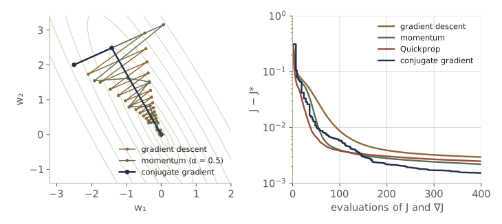
Measured fairly, in evaluations of the error and gradient, all three accelerated methods beat plain gradient descent at every budget. Quickprop is fastest at the start, where its per-weight curvature estimates pay off quickly; momentum catches up with it by 100 evaluations; and conjugate gradient, whose line searches cost several evaluations each, reaches the lowest error by 400 evaluations, once the surface near the minimum is close to quadratic. On larger problems the ranking can change (stochastic methods can win when the training set is large and redundant, since conjugate gradient needs the full batch gradient), but for small and moderate networks trained in batch mode, conjugate gradient is a strong default.
Additional networks and training methods
DHS close the methods part of the chapter with a tour of other architectures and training schemes that work well on particular classes of problems. We treat them briefly, with code where a small example makes the idea concrete.
Radial basis function networks
A radial basis function (RBF) network replaces the sigmoid hidden units by units with localized responses, typically Gaussians centered at points \(\boldsymbol{\mu}_j\), and uses linear output units:
\[z_k(\mathbf{x}) = \sum_{j=0}^{n_H} w_{kj}\, \varphi_j(\mathbf{x}), \qquad \varphi_j(\mathbf{x}) = \exp\left( -\frac{\lVert \mathbf{x} - \boldsymbol{\mu}_j \rVert^2}{2\sigma^2} \right), \quad \varphi_0 = 1 .\]If the centers and width are fixed, the outputs are linear in the weights. Stacking the hidden outputs of all training patterns as the rows of a matrix \(\boldsymbol{\Phi}\) and the targets as the rows of \(\mathbf{T}\), minimizing \(\sum_m \lVert \mathbf{z}(\mathbf{x}_m) - \mathbf{t}_m \rVert^2\) is the least-squares problem of module 05, with solution \(\mathbf{W}^{t} = \boldsymbol{\Phi}^{\dagger}\mathbf{T}\) given by the pseudoinverse, no gradient descent needed. The centers can be chosen by clustering (module 10), but a simpler choice is a random subset of the training patterns, which we use here. With a nonlinear output unit, backpropagation trains the output weights, and even the centers and widths, since derivatives of the Gaussians are easy to take.
def rbf_features(X, centers, sigma):
    d2 = np.sum((X[:, None, :] - centers[None, :, :]) ** 2, axis=2)
    return augment(np.exp(-d2 / (2 * sigma ** 2)))            # phi_0 = 1 plus the Gaussians

def train_rbf(X, T, n_centers, sigma, rng):
    centers = X[rng.choice(len(X), n_centers, replace=False)]  # centers taken from the data
    W = np.linalg.lstsq(rbf_features(X, centers, sigma), T, rcond=None)[0]   # least-squares outputs
    return centers, W

print(" centers   train error   test error (mean over 5 draws of centers)")
for M in [2, 4, 8, 16, 32, 64]:
    errs = []
    for draw in range(5):
        centers, W = train_rbf(X_nx, T_nx, M, 0.7, np.random.default_rng(60 + draw))
        pred = lambda X: (rbf_features(X, centers, 0.7) @ W)[:, 0] < 0
        errs.append((np.mean(pred(X_nx) != (y_nx == 1)), np.mean(pred(X_nxt) != (y_nxt == 1))))
    tr, te = np.mean(errs, axis=0)
    print(f"{M:8d}   {tr:11.3f}   {te:10.3f}")
print(f"2-4-1 network, backpropagation: test error = {np.mean(classify(W1_b, W2_b, X_nxt) != y_nxt):.3f}")
 centers   train error   test error (mean over 5 draws of centers)
       2         0.247        0.269
       4         0.195        0.205
       8         0.052        0.075
      16         0.027        0.050
      32         0.019        0.045
      64         0.021        0.055
2-4-1 network, backpropagation: test error = 0.057
Two or four centers are not enough, because a random handful of training points rarely covers all four blobs of the noisy XOR. Eight centers come close, and from sixteen on the RBF network matches the backpropagation network, with training that consists of one least-squares solve. (With 64 centers of this width the fit starts to follow the noise.) RBF networks are most natural when the data form clusters, and they give a local representation, in contrast to the distributed representation of sigmoid units. The price of the linear solve is that the whole matrix \(\boldsymbol{\Phi}\) must be handled at once, which limits it to problems of moderate size.
Special bases
Sometimes we know the functional form of the class-conditional densities, for example that each class is a mixture of two Gaussians. Then it makes sense to use hidden units that match that form, such as Gaussian units whose means and covariances are the parameters, and train them with a rule that estimates those parameters. Fewer parameters are needed for the same quality of fit. In the language of module 09, a special basis raises the bias of the model to lower its variance; in the language of module 03, it is close to fitting a parametric model by maximum likelihood.
Matched filters
Suppose we want to detect a known signal \(x(t)\) with a linear detector. A linear detector is characterized by its time-reversed impulse response \(w(t)\), and its output when the signal is offset by \(T\) is
\[z(T) = \int_{-\infty}^{\infty} x(t)\, w(t - T)\, dt .\]Which \(w\) gives the largest response? Scaling \(w\) scales \(z\), so we fix the filter’s energy, \(\int w^2(t)\, dt = E\), and ask for the best shape. Set \(T = 0\) and introduce a Lagrange multiplier \(\lambda\) for the constraint. The functional \(\int [x(t) w(t) - \lambda w^2(t)]\, dt\) must be stationary under every small change \(\delta w(t)\), which requires \(x(t) - 2\lambda w(t) = 0\) for all \(t\). So
\[w(t) \propto x(t) :\]the best detector is a copy of the signal itself, the matched filter, with the constant set by the energy. That this is a maximum and not just a stationary point follows from the Cauchy–Schwarz inequality, \(z(0) = \int x w\, dt \le \sqrt{\int x^2 dt}\,\sqrt{E}\), with equality exactly when \(w\) is proportional to \(x\). The discrete version is the same with sums, and the cell checks it: the matched filter’s peak response equals the bound \(\lVert \mathbf{x} \rVert \sqrt{E}\), random filters of the same energy do worse, and the matched filter finds the signal’s position in noise.
t_sig = np.arange(40)
x_sig = np.sin(2 * np.pi * t_sig / 10) * np.exp(-((t_sig - 20) / 8.0) ** 2)   # the known signal
E = 1.0
w_match = np.sqrt(E) * x_sig / np.linalg.norm(x_sig)                         # matched filter
peak = lambda w: np.max(np.correlate(x_sig, w, mode="full"))                 # max over offsets T
filt_rng = np.random.default_rng(71)
random_peaks = []
for _ in range(1000):
    w = filt_rng.standard_normal(40)
    random_peaks.append(peak(np.sqrt(E) * w / np.linalg.norm(w)))
print(f"bound ||x|| sqrt(E) = {np.linalg.norm(x_sig) * np.sqrt(E):.4f}")
print(f"matched filter peak = {peak(w_match):.4f}")
print(f"best of 1000 random filters with the same energy = {max(random_peaks):.4f}")

stream = 0.3 * filt_rng.standard_normal(300)
stream[170:210] += x_sig                                                   # signal hidden at offset 170
response = np.correlate(stream, w_match, mode="valid")
print("offset of the largest matched-filter response:", int(np.argmax(response)))
bound ||x|| sqrt(E) = 2.2390
matched filter peak = 2.2390
best of 1000 random filters with the same energy = 1.3343
offset of the largest matched-filter response: 170
The connection to networks is the one noted under hidden-layer representations: a hidden unit responds most strongly to inputs that match its weight vector, so a hidden unit is a (nonlinear) matched filter for the pattern its weights encode.
Convolutional networks
We can build prior knowledge into the architecture. If a classifier should not care where in the input a pattern occurs, we can replicate the same detector at every position. This is the idea of the time delay neural network (TDNN), developed for speech: each hidden unit looks at only a short window of the input, hidden units at later positions look at correspondingly shifted windows, and all of them use the same weights. Forcing weights to be equal is called weight sharing. Training is ordinary backpropagation with one extra rule: the gradient for a shared weight is the sum of the gradients of all its copies, because the error depends on the shared weight through every position where it is used. The same construction in two spatial dimensions gives the convolutional networks used for character and image recognition, where the location of a pattern in the image is not precisely known.
A tiny one-dimensional example shows both properties. The hidden layer is a convolution of the input with a 3-tap kernel \(\mathbf{v}\) plus a bias, followed by the scaled tanh, and the output takes the maximum over positions.
def conv_net(v, v0, x):
    """Hidden y_t = f(sum_s v_s x_{t+s} + v0) at each valid position t; output z = sum_t y_t."""
    net_t = np.array([v @ x[t:t + len(v)] for t in range(len(x) - len(v) + 1)]) + v0
    y_t = TANH.f(net_t)
    return net_t, y_t, y_t.sum()

v, v0 = np.array([1.0, -2.0, 1.0]), 0.5                   # shared kernel and bias: 4 weights in all
x_pat = np.zeros(12); x_pat[3:6] = [-1.0, 1.0, -0.5]      # a short pattern at position 3
x_shift = np.roll(x_pat, 4)                               # the same pattern 4 steps later
net_a, y_a, z_a = conv_net(v, v0, x_pat)
_, y_b, z_b = conv_net(v, v0, x_shift)
print("hidden, pattern at 3:", np.round(y_a, 2))
print("hidden, pattern at 7:", np.round(y_b, 2))
print(f"outputs: {z_a:.4f} and {z_b:.4f}")

# Untied copies: position t has its own kernel copy, with gradient dz/dv^(t)_s = f'(net_t) x_{t+s}
grad_copies = np.array([TANH.df(net_a[t]) * x_pat[t:t + 3] for t in range(len(net_a))])
g_num = numerical_gradient(lambda vv: conv_net(vv, v0, x_pat)[2], v)
print("sum of the copies' gradients:", np.round(grad_copies.sum(axis=0), 6))
print("numerical gradient, shared v:", np.round(g_num, 6))
hidden, pattern at 3: [ 0.55 -0.55  1.68 -1.65  1.6   0.    0.55  0.55  0.55  0.55]
hidden, pattern at 7: [ 0.55  0.55  0.55  0.55  0.55 -0.55  1.68 -1.65  1.6   0.  ]
outputs: 3.8344 and 3.8344
sum of the copies' gradients: [-0.5006 -0.0375 -1.0239]
numerical gradient, shared v: [-0.5006 -0.0375 -1.0239]
Shifting the input shifts the hidden layer by the same amount (equivariance), and adding the hidden outputs over positions makes the output invariant to the shift, as long as the pattern stays inside the input window (taking the maximum over positions, max pooling, works the same way). The detector has 4 weights where an unshared layer of the same size would have 40, and the derivative with respect to a shared weight is the sum of the derivatives of its ten copies, as the last two lines confirm.
Recurrent networks
So far information has flowed only forward; the only backward flow was of error signals during training. Recurrent networks have feedback connections. In their general form they are used mostly for time series, but one simple type has been used for static classification: the output values are fed back as extra inputs alongside the features. A pattern \(\mathbf{x}\) is presented, the outputs are computed and fed back, the hidden units respond to \(\mathbf{x}\) and the previous outputs, and so on until the outputs stop changing; the final outputs classify the pattern. Unfolded over the iterations, the network is equivalent to a deep feedforward network in which the same weights are repeated in every layer, so it can be trained by backpropagation with weight sharing, as for the convolutional network, a method known as backpropagation through time. Recurrent networks learn structure that spans short stretches of time well. They struggle with longer-range structure, because the error signal is weakened each time it passes back through a layer of the unfolded network.
Cascade-correlation
Cascade-correlation grows the network during training instead of fixing its size in advance. It starts with no hidden units, inputs connected directly to outputs, and trains those weights on an LMS criterion. If the error is low enough it stops. Otherwise it adds one hidden unit, connected to all inputs and to the outputs, freezes the weights trained so far, and trains only the new unit’s weights. Each later hidden unit also receives the outputs of all earlier hidden units, which lets it build on features already found rather than repeat them, and the network becomes a cascade of units each one layer deeper than the last. Units are added until the training error is acceptable. Because only a few weights are trained at a time, training is often faster than backpropagation on a fixed network. (In Fahlman and Lebiere’s original algorithm, a candidate unit is first trained to maximize the correlation between its output and the remaining error, which gives the method its name; DHS describe a simplified version.)
Regularization, complexity adjustment, and pruning
The inputs and outputs of a network are fixed by the problem, but the number of hidden units and weights is not. Too many weights trained too long overfit; too few cannot learn the training set. One general remedy is regularization: a criterion that adds to the training error a term that penalizes complexity,
\[J = J_{pat} + \lambda J_{reg},\]where \(\lambda\) sets the strength of the penalty. Weight decay is of this form, with \(J_{reg}\) proportional to \(\mathbf{w}^{t}\mathbf{w}\). Another remedy is pruning: train a network that is large enough, then remove the weights that are least needed. The obvious rule, remove the smallest weights, can work but is not optimal, since a small weight can matter a great deal if the error is sensitive to it. Pruning should instead estimate each weight’s importance, in the spirit of the Wald statistic of classical statistics, and remove the least important one.
Optimal Brain Damage and Optimal Brain Surgeon
Both methods start from a network trained to a local minimum \(\mathbf{w}^*\) and use the second-order expansion of the error for a weight change \(\delta\mathbf{w}\),
\[\delta J = \left( \frac{\partial J}{\partial \mathbf{w}} \right)^{t} \delta\mathbf{w} + \frac12 \delta\mathbf{w}^{t}\mathbf{H}\,\delta\mathbf{w} + O(\lVert \delta\mathbf{w} \rVert^3) \approx \frac12 \delta\mathbf{w}^{t}\mathbf{H}\,\delta\mathbf{w},\]since the gradient vanishes at a minimum. Deleting weight \(q\) means imposing \(w_q + \delta w_q = 0\), which we write as \(\mathbf{u}_q^{t}\delta\mathbf{w} + w_q = 0\) with \(\mathbf{u}_q\) the unit vector along weight \(q\). Optimal Brain Surgeon (OBS) lets all the other weights adjust to compensate and asks for the smallest increase in error. Minimize \(\tfrac12 \delta\mathbf{w}^{t}\mathbf{H}\delta\mathbf{w}\) subject to the constraint, with multiplier \(\lambda\): stationarity gives \(\mathbf{H}\delta\mathbf{w} + \lambda\mathbf{u}_q = \mathbf{0}\), so \(\delta\mathbf{w} = -\lambda\mathbf{H}^{-1}\mathbf{u}_q\), and the constraint gives \(\lambda = w_q / [\mathbf{H}^{-1}]_{qq}\). Therefore
\[\delta\mathbf{w} = -\frac{w_q}{[\mathbf{H}^{-1}]_{qq}}\, \mathbf{H}^{-1}\mathbf{u}_q, \qquad L_q = \frac12 \delta\mathbf{w}^{t}\mathbf{H}\,\delta\mathbf{w} = \frac{w_q^2}{2\,[\mathbf{H}^{-1}]_{qq}} .\]\(L_q\) is the saliency of weight \(q\): the predicted increase in error when it is removed and the others are adjusted by \(\delta\mathbf{w}\). OBS removes the weight with the smallest saliency, applies the adjustment, and repeats. Optimal Brain Damage (OBD), its predecessor, assumes \(\mathbf{H}\) is diagonal. Then no other weight adjusts, and the saliency is \(L_q = \tfrac12 H_{qq} w_q^2\), which is cheaper to compute but ignores the ability of correlated weights to take over for one another.
We apply both to the band network from the Hessian section, where the three weights from the irrelevant input \(x_2\) should be expendable. First we polish the minimum with conjugate gradients on the criterion including its decay term (the saliency formulas assume a zero gradient). Then for every weight we compare the predicted saliencies with the actual increase in the criterion: for OBD, setting the weight to zero; for OBS, applying the full adjustment \(\delta\mathbf{w}\). The indices follow pack: 0–8 are input-to-hidden weights (for each hidden unit, bias, \(x_1\), \(x_2\)), 9–12 are hidden-to-output weights (bias, then hidden units 1–3).
lam_band = 1e-4 / 0.2                                        # epsilon / eta of the decay used above
def fg_band(w):
    J, g1, g2 = backprop(*unpack(w, 2, 3, 1), X_band, T_band)
    return J / 200 + 0.5 * lam_band * w @ w, pack(g1, g2) / 200 + lam_band * w

w_opt, _ = conjugate_gradient(fg_band, w_bd, 1500)
J_opt, g_opt = fg_band(w_opt)
H = hessian_fd(lambda w: fg_band(w)[1], w_opt)
H_inv = np.linalg.inv(H)
L_obd = 0.5 * np.diag(H) * w_opt ** 2
L_obs = w_opt ** 2 / (2 * np.diag(H_inv))
actual_obd, actual_obs = [], []
for q in range(len(w_opt)):
    w_zero = w_opt.copy(); w_zero[q] = 0.0
    actual_obd.append(fg_band(w_zero)[0] - J_opt)
    dw = -w_opt[q] / H_inv[q, q] * H_inv[:, q]              # OBS adjustment (sets w_q to zero)
    actual_obs.append(fg_band(w_opt + dw)[0] - J_opt)
print(f"J = {J_opt:.4f}, gradient norm = {np.linalg.norm(g_opt):.1e}")
print("  q    w_q     OBD pred   OBD actual   OBS pred   OBS actual")
for q in np.argsort(L_obs):
    print(f"{q:3d} {w_opt[q]:7.3f}   {L_obd[q]:8.4f}   {actual_obd[q]:10.4f}"
          f"   {L_obs[q]:8.4f}   {actual_obs[q]:10.4f}")
print("first weight to prune:  magnitude ->", np.argmin(np.abs(w_opt)), "  OBD ->", np.argmin(L_obd),
      "  OBS ->", np.argmin(L_obs))
J = 0.1557, gradient norm = 5.3e-09
  q    w_q     OBD pred   OBD actual   OBS pred   OBS actual
  2  -0.007     0.0000       0.0000     0.0000       0.0000
  9   0.414     0.0646       0.0669     0.0002       0.0003
  5   0.192     0.0015       0.0018     0.0012       0.0015
  8   0.217     0.0057       0.0051     0.0017       0.0101
 12  -1.088     1.1176       0.7654     0.0034       0.0131
  7   0.944     0.1006       0.0203     0.0063       0.2086
  6   2.841     0.2827       0.7767     0.0076       0.5283
  4  -3.946     0.3865       0.3704     0.0103       0.2869
  3   3.449     0.4659       0.4003     0.0133       0.5494
  1   4.253     0.8064       0.4898     0.0137       0.7964
  0   3.549     0.8707       0.5413     0.0168       1.1386
 10   0.798     0.5276       0.6405     0.0226       0.4320
 11   0.609     0.3084       0.3822     0.0710       0.7890
first weight to prune:  magnitude -> 2   OBD -> 2   OBS -> 2
The rows are sorted by OBS saliency, and the top of the table is where pruning happens. All three rules agree on the first weight, the nearly zero weight 2 from \(x_2\). For the first few rows the predictions match the actual increases well, and OBD ranks the three \(x_2\) weights (indices 2, 5, 8) as its three cheapest. OBS finds something OBD cannot see: the output bias (index 9) can be removed at almost no cost if the other weights compensate, while OBD, which does not let the other weights move, predicts a sizable increase for it, correctly for its own no-compensation rule. By the fourth row the OBS prediction is already off by a factor of about six, and further down the table the predictions degrade badly. Removing an important weight is not a small perturbation, and the quadratic model is only trustworthy for the small changes that pruning is meant to make, which is why OBS removes one weight at a time and retrains or recomputes between removals.
OBS needs \(\mathbf{H}^{-1}\). With the outer-product approximation it can be built one pattern at a time without ever inverting a matrix. Start from \(\mathbf{H}_0^{-1} = \alpha^{-1}\mathbf{I}\) with a small \(\alpha\) (in effect a weight-decay term), and add the patterns’ contributions \(\frac1n \mathbf{X}\mathbf{X}^{t}\) one by one with the Sherman–Morrison formula for a rank-one update:
\[\mathbf{H}_{m+1}^{-1} = \mathbf{H}_m^{-1} - \frac{\mathbf{H}_m^{-1}\mathbf{X}^{[m+1]}\mathbf{X}^{[m+1]t}\mathbf{H}_m^{-1}}{n + \mathbf{X}^{[m+1]t}\mathbf{H}_m^{-1}\mathbf{X}^{[m+1]}} .\]After all \(n\) patterns, \(\mathbf{H}_n^{-1}\) is the inverse of \(\alpha\mathbf{I} + \frac1n\sum_m \mathbf{X}^{[m]}\mathbf{X}^{[m]t}\).
alpha_h = 1e-4
Jac = output_jacobian(*unpack(w_opt, 2, 3, 1), X_band)
H_inv_rec = np.eye(Jac.shape[1]) / alpha_h
for Xm in Jac:                                              # one pattern at a time
    HX = H_inv_rec @ Xm
    H_inv_rec -= np.outer(HX, HX) / (len(Jac) + Xm @ HX)
H_direct = alpha_h * np.eye(Jac.shape[1]) + Jac.T @ Jac / len(Jac)
print(f"max relative difference from the direct inverse: "
      f"{np.max(np.abs(H_inv_rec @ H_direct - np.eye(len(H_direct)))):.1e}")
L_rec = w_opt ** 2 / (2 * np.diag(H_inv_rec))
print("weight OBS would prune first with the approximate inverse:", np.argmin(L_rec))
max relative difference from the direct inverse: 6.1e-12
weight OBS would prune first with the approximate inverse: 2
The recursion reproduces the inverse to rounding error, and the approximate Hessian leads to the same choice of weight to prune. Pruning algorithms like these can be read as priors that favor networks with few weights, a view developed with the other methods for choosing model complexity in module 09.
Summary
| Method | What it assumes or uses | How it is trained or decides |
|---|---|---|
| Three-layer network, threshold units | hand-designed hidden features | fixed weights; the sign of \(z\) |
| Three-layer network, sigmoid units | differentiable \(f\); enough hidden units | backpropagation: \(\Delta w_{kj} = \eta\delta_k y_j\), \(\Delta w_{ji} = \eta\delta_j x_i\) |
| Stochastic / batch / on-line protocols | a stored training set / the same / a stream | one random pattern / all patterns / each pattern once per update |
| Squared error, 0–1 targets | large \(n\), enough hidden units | outputs approximate \(P(\omega_k \mid \mathbf{x})\) |
| Softmax with cross-entropy | outputs are class probabilities | \(\delta_k = t_k - z_k\); outputs sum to 1 |
| Momentum | narrow valleys, plateaus | \((1-\alpha)\Delta\mathbf{w}_{bp} + \alpha\Delta\mathbf{w}(m-1)\) |
| Weight decay, stopped training | small weights generalize better | shrink \(\mathbf{w}\) by \(1 - \epsilon\); stop at the validation minimum |
| Newton, Quickprop | a locally quadratic error | \(-\mathbf{H}^{-1}\nabla J\); per-weight parabola |
| Conjugate gradient | batch gradient, line searches | \(-\nabla J + \beta_m\Delta\mathbf{w}(m-1)\), Polak–Ribière \(\beta_m\) |
| RBF network | localized (clustered) structure | centers from data, output weights by least squares |
| Convolutional / TDNN | translation invariance | weight sharing; shared gradient is a sum over positions |
| OBD / OBS pruning | quadratic error near a minimum | remove the weight with the smallest saliency \(w_q^2 / (2[\mathbf{H}^{-1}]_{qq})\) |
Ideas to carry forward:
- A multilayer network is a linear discriminant in a learned feature space. The hidden units remap the inputs until the classes are linearly separable, and backpropagation’s hidden sensitivities \(\delta_j = f'(net_j)\sum_k w_{kj}\delta_k\) are what make that remapping learnable.
- Trained on squared error or cross-entropy with 1-of-\(c\) targets and enough data, a network estimates posterior probabilities, which connects it to the Bayes decision theory of module 02. With finite data it is an approximation that is best where \(p(\mathbf{x})\) is large.
- Most of the practical heuristics are about conditioning: standardized inputs, antisymmetric sigmoids, and scaled initial weights keep the Hessian’s eigenvalues in a narrow range, and momentum, Quickprop, and conjugate gradients cope with the spread that remains.
- Complexity control is the central practical problem: the number of hidden units, weight decay, stopped training, and pruning are all ways to trade training error against generalization, a trade-off that module 09 studies in general.
Exercises
- Show that if every hidden unit of a three-layer network has a linear activation function, the network computes a linear function of \(\mathbf{x}\), so it is no more powerful than a two-layer network. What happens if only the output units are linear?
- Build a network of threshold units for three-bit parity (output \(+1\) when an odd number of the inputs \(x_1, x_2, x_3 \in \{-1, +1\}\) are \(+1\)). How few hidden units can you use? Verify your weights on all eight patterns with
forwardandsgn. - Extend the backpropagation derivation to a network with two hidden layers, and implement it by generalizing
forwardandbackpropto a list of weight matrices. Verify your gradient withnumerical_gradientand train a 2-4-4-1 network on the noisy XOR. Then take a trained 2-2-1 XOR network and confirm that all \(2! \times 2^2\) permutations and sign flips of its hidden units give the same error. - For the logistic sigmoid \(f(net) = 1/(1 + e^{-net})\), show that \(f' = f(1 - f)\); for \(f = a\tanh(b\,net)\), show that \(f' = (b/a)(a^2 - f^2)\). Explain why these identities make the backward pass cheaper.
- Fill in the steps of the derivation that a squared-error network approximates the posteriors, and redo it for \(\pm 1\) targets to show that the outputs approximate \(2P(\omega_k \mid \mathbf{x}) - 1\). Then check that claim numerically by training the 1-6-3 network with tanh outputs and \(\pm 1\) targets.
- Show that for a quadratic criterion \(J = \tfrac12 \mathbf{w}^{t}\mathbf{H}\mathbf{w}\), gradient descent converges for every starting point exactly when \(0 < \eta < 2/\lambda_{\max}\), and that the best fixed learning rate gives the convergence factor \((\kappa - 1)/(\kappa + 1)\). Compare with the iteration counts in the momentum experiment.
- Derive the Quickprop update from the assumption that \(J\) is a parabola in one weight, and show that it is the secant method applied to \(\partial J/\partial w = 0\).
- Show that on a quadratic criterion with exact line searches, successive gradients in conjugate gradient descent are orthogonal, and use this to prove that the Fletcher–Reeves and Polak–Ribière values of \(\beta_m\) agree.
- Derive the OBS formulas for \(\delta\mathbf{w}\) and \(L_q\) with a Lagrange multiplier, as in the notes, and show that when \(\mathbf{H}\) is diagonal they reduce to OBD. Then write a loop that prunes the band network one weight at a time with OBS (recomputing \(\mathbf{H}\) over the remaining weights after each removal and polishing with a few conjugate gradient steps), and plot the training and test error against the number of weights removed. Compare with pruning by magnitude.
- Train RBF networks on the noisy XOR with the centers chosen by k-means (module 10) instead of at random, for the same numbers of centers. Also vary \(\sigma\) over a grid. Which choice matters more?
- Implement the recurrent classifier described in the notes: a 2-4-1 network whose output is fed back as a third input, iterated five times per pattern. Unfold it into a five-layer network with shared weights, train it by backpropagation with summed gradients for the shared weights, and check your gradient numerically.
- In your own words: why can a network with more hidden units than necessary be both easier to train (fewer bad local minima) and worse at generalization? Which of the techniques in this module address each half of that statement?
Going further
- R. O. Duda, P. E. Hart, and D. G. Stork, Pattern Classification, 2nd ed., chapter 6. Problems 1–2 (expressive power), 3–11 (backpropagation), 12–16 (error surfaces and convergence), 17–22 (posteriors and softmax), 26–30 (practical techniques), 31–35 (Hessian, Quickprop, conjugate gradients), 36–38 (matched filters, OBD/OBS, RBF), and 39–45 (regularization and OBS) pair with the sections above; computer exercises 1–12 follow the same order.
- D. E. Rumelhart, G. E. Hinton, and R. J. Williams, “Learning representations by back-propagating errors”, Nature, 1986 — the paper that brought backpropagation to a wide audience, with XOR among its examples.
- G. Cybenko, “Approximation by superpositions of a sigmoidal function”, Mathematics of Control, Signals and Systems, 1989 — a universal approximation theorem for three-layer sigmoid networks.
- M. D. Richard and R. P. Lippmann, “Neural network classifiers estimate Bayesian a posteriori probabilities”, Neural Computation, 1991 — the posterior result of the Bayes section, with experiments.
- Y. LeCun, L. Bottou, G. B. Orr, and K.-R. Müller, “Efficient BackProp”, in Neural Networks: Tricks of the Trade, Springer, 1998 — the practical heuristics (input standardization, the scaled tanh, initialization, learning rates) with their reasoning; C. M. Bishop, Neural Networks for Pattern Recognition, Oxford, 1995, covers second-order methods, RBF networks, and pruning at greater length.
- Intro to ML, module 05 derives backpropagation, the Hessian and its approximations, regularization, and Bayesian neural networks in Bishop’s notation; Intro to ML, module 04 covers the softmax and cross-entropy for linear models.
These notes follow the chapters of R. O. Duda, P. E. Hart, and D. G. Stork, Pattern Classification, 2nd edition (Wiley, 2001), the course text. The explanations, code, figures, and exercises here are written for this course; the book remains the reference, with the full derivations, worked examples, and many more problems.