CSE 455/555 · Module 07 · Session 7
Stochastic Methods
Simulated annealing and its deterministic variant, Boltzmann machines and Boltzmann learning, genetic algorithms, and genetic programming.
Companion reading: Duda, Hart & Stork, Pattern Classification, chapter 7, “Stochastic Methods”
By the end of this module you can
- Write the energy of a network of \(\pm 1\) units with symmetric weights, find its minimum by brute force on a small network, and explain why greedy single-unit descent stops in local minima.
- State the Boltzmann distribution and its limits at high and low temperature, show that the Metropolis acceptance rule leaves it invariant, and implement stochastic simulated annealing with a geometric cooling schedule.
- Derive the mean-field update \(m_i = \tanh(l_i/T)\), implement deterministic annealing, and explain its critical temperature and why its minima lie at corners of the hypercube.
- Derive the Boltzmann learning rule as gradient descent on a Kullback–Leibler divergence, check it against exact enumeration, and explain why some target distributions need hidden units.
- Use a trained Boltzmann network to classify, to handle missing features, and to complete patterns, and approximate its learning with deterministic (mean-field) Boltzmann learning.
- Choose the practical settings of a Boltzmann network — hidden units, initial weights, initial temperature from an acceptance ratio, learning rate — and relate a Boltzmann chain to a hidden Markov model.
- Implement a genetic algorithm for feature selection, compare selection schemes against the true optimum, and explain the schema argument for why crossover can help.
- Represent programs as expression trees, implement the genetic-programming operators, and evolve a small expression that fits a target.
Contents
- Why stochastic methods
- Stochastic search
- Boltzmann learning
- Boltzmann networks and graphical models
- Evolutionary methods
- Genetic programming
- Summary
- Exercises
- Going further
So far every classifier in this course has been trained the same way: write down a criterion, then find its best parameters with a closed form (the maximum-likelihood estimates of module 03) or by following its gradient (the linear machines of module 05 and backpropagation in module 06). That works when the criterion is smooth and its local optima are few or harmless. It breaks down when the parameters are discrete, when the space of candidates is astronomically large, or when the criterion has so many poor local optima that a downhill method almost always stops in one.
This module collects methods that use randomness on purpose to get around those obstacles. Chapter 7 of Duda, Hart & Stork’s Pattern Classification (DHS from here on) groups them into two families. The first comes from statistical physics: simulated annealing searches for low-energy configurations of a network of binary units by accepting some uphill moves, with a “temperature” that controls how many; Boltzmann learning turns the same network into a probabilistic model whose weights are trained so that the network’s random behavior matches the data. The second family comes from biology: genetic algorithms and genetic programming keep a population of candidate classifiers, score them, and breed the better ones.
Three small running examples make every claim checkable. A 12-unit network has only 4096 configurations, so we can find its true minimum by brute force and see exactly when annealing succeeds. Boltzmann machines with at most 7 units have at most 128 states, so we can compute their probabilities exactly and verify the learning rule against the gradient of the divergence it is meant to reduce. A 16-feature selection problem has 65,535 nonempty feature subsets, few enough to score every one and see how close the genetic algorithm gets. The sampling side of these ideas — Markov chains, the Metropolis algorithm, Gibbs sampling — is developed at more length in Intro to ML, module 11.
Why stochastic methods
A model with a handful of continuous parameters and a smooth criterion is a friendly search problem: set the derivative to zero or walk downhill. As models grow, three things go wrong. The criterion acquires many local optima, so the answer depends on the starting point, and the usual fix — restart from several random points — gives no assurance that any of them reached a good optimum. Some parameters are discrete (which features to use, which units are connected, what shape an expression has), so there is no derivative at all. And exhaustive search, the only method guaranteed to succeed, grows exponentially with the number of discrete choices.
The methods of this module bias a search toward regions where good solutions are likely while keeping enough randomness to escape poor ones. They cost a great deal of computation, and they come with weaker guarantees than the methods of earlier modules; DHS present them, and we follow, on problems small enough that simpler methods would also work, so that we can see what the randomness buys. The physics-inspired family has a clean probabilistic theory and gets most of our attention; the evolutionary family is more heuristic but very flexible.
The first cell sets up NumPy and two helpers we use throughout: one lists every vector in \(\{-1, +1\}^n\), the other evaluates the network energy defined in the next section for many configurations at once.
import itertools
import numpy as np
from scipy.special import logsumexp, expit

np.set_printoptions(precision=4, suppress=True)
rng = np.random.default_rng(455)

def all_pm1(n):
    """All 2^n vectors in {-1, +1}^n, one per row (the first column varies slowest)."""
    return np.array(list(itertools.product([-1.0, 1.0], repeat=n)))

def energy(S, W):
    """E = -1/2 sum_ij w_ij s_i s_j for every configuration in S (shape (..., N))."""
    return -0.5 * np.einsum('...i,ij,...j->...', S, W, S)

print(all_pm1(2))
[[-1. -1.]
 [-1.  1.]
 [ 1. -1.]
 [ 1.  1.]]
Stochastic search
An energy over binary units
We have \(N\) variables \(s_1, \dots, s_N\), each equal to \(+1\) or \(-1\), and a symmetric matrix of weights \(w_{ij} = w_{ji}\) that may be positive or negative, with \(w_{ii} = 0\). The energy of a configuration \(\mathbf{s} = (s_1, \dots, s_N)\) is
\[E(\mathbf{s}) = -\frac{1}{2} \sum_{i=1}^{N} \sum_{j=1}^{N} w_{ij} s_i s_j = -\frac{1}{2}\mathbf{s}^{t}\mathbf{W}\mathbf{s},\]and the task is to find a configuration of lowest energy. A positive \(w_{ij}\) rewards units \(i\) and \(j\) for agreeing (the product \(s_i s_j = +1\) lowers the energy); a negative one rewards them for disagreeing. When some weights pull in incompatible directions — \(w_{12} > 0\), \(w_{23} > 0\), \(w_{13} < 0\) cannot all be satisfied — the problem is called frustrated, and that is what makes it hard. We picture it as a network: one node per variable, called a unit, and an undirected link between \(i\) and \(j\) whenever \(w_{ij} \ne 0\). The physical picture behind the vocabulary is a set of tiny magnets whose north poles point up (\(+1\)) or down (\(-1\)), with interaction strengths \(w_{ij}\).
Two remarks about the form. The self-weights are set to zero because \(w_{ii}s_i^2 = w_{ii}\) adds a constant that does not depend on the configuration. A nonsymmetric matrix could be replaced by its symmetric part \(\tfrac{1}{2}(\mathbf{W} + \mathbf{W}^{t})\) without changing any energy, so assuming symmetry costs nothing (Exercise 1). And since \(E(-\mathbf{s}) = E(\mathbf{s})\), minima always come in mirror-image pairs.
The quantity that drives everything below is the local field (DHS call it the net force) on unit \(i\),
\[l_i = \sum_{j} w_{ij} s_j .\]The terms of \(E\) that involve \(s_i\) are \(-s_i l_i\) (the pair \((i, j)\) appears twice in the double sum, cancelling the \(\tfrac{1}{2}\)). So flipping unit \(i\) from \(s_i\) to \(-s_i\) changes the energy by
\[\Delta E_i = E(\text{after}) - E(\text{before}) = s_i l_i - (-s_i l_i) = 2 s_i l_i ,\]which needs only the weights into unit \(i\), not the whole energy. Unit \(i\) “wants” to point along its field: \(s_i = \operatorname{sgn}(l_i)\) gives the lower of its two energies.
Our running network has \(N = 12\) units and weights drawn once from a standard normal and rounded to one decimal. With 12 units there are \(2^{12} = 4096\) configurations, so we can list them all.
N = 12
rng_w = np.random.default_rng(12)
A = np.round(rng_w.normal(0.0, 1.0, size=(N, N)), 1)
W = np.triu(A, 1)
W = W + W.T                         # symmetric, zero diagonal

S_all = all_pm1(N)                  # all 4096 configurations
E_all = energy(S_all, W)
E_min = E_all.min()
ground = np.flatnonzero(np.isclose(E_all, E_min))
print(f"{len(S_all)} configurations, energies from {E_min:.2f} to {E_all.max():.2f}")
print("global minima:")
for k in ground:
    print("  ", S_all[k].astype(int), f"E = {E_all[k]:.2f}")
4096 configurations, energies from -22.50 to 27.10
global minima:
   [-1 -1 -1 -1 -1  1 -1  1 -1 -1  1 -1] E = -22.50
   [ 1  1  1  1  1 -1  1 -1  1  1 -1  1] E = -22.50
As promised, the two global minima are mirror images. Brute force is fine here, but each extra unit doubles the work: at a billion configurations per second, \(N = 60\) would already take decades. We need search methods whose cost does not grow like \(2^N\).
Greedy descent and local minima
The obvious search is greedy: start from a random configuration, visit the units one at a time, and set each to the sign of its local field, repeating until no unit changes. Each change strictly lowers the energy (it flips a unit with \(\Delta E_i < 0\)), there are finitely many configurations, so the procedure must stop, and it stops at a local minimum: a configuration where no single flip lowers the energy, that is, \(s_i l_i \ge 0\) for every \(i\). The same procedure appears in image de-noising with an Ising model under the name iterated conditional modes (Intro to ML, module 08).
How many local minima does our network have, and how often does greedy descent find the global one?
L_all = S_all @ W                   # local fields l_i for every configuration
dE_all = 2 * S_all * L_all          # energy change if unit i were flipped
is_local_min = np.all(dE_all >= 0, axis=1)
print(f"{is_local_min.sum()} single-flip local minima, energies:")
print(np.round(np.sort(E_all[is_local_min]), 2))

def greedy_descent(S, W, max_sweeps=100):
    """Set each unit to the sign of its local field, in order, until nothing changes.
    S holds R independent starting configurations, one per row."""
    S = S.copy()
    for _ in range(max_sweeps):
        changed = False
        for i in range(W.shape[0]):
            l = S @ W[i]
            new = np.where(l > 0, 1.0, np.where(l < 0, -1.0, S[:, i]))
            changed = changed or bool(np.any(new != S[:, i]))
            S[:, i] = new
        if not changed:
            break
    return S

S0 = rng.choice([-1.0, 1.0], size=(1000, N))
E_greedy = energy(greedy_descent(S0, W), W)
print(f"greedy descent reached the global minimum from {np.mean(np.isclose(E_greedy, E_min)):.1%} of 1000 starts")
vals, counts = np.unique(np.round(E_greedy, 2), return_counts=True)
for v, c in zip(vals, counts):
    print(f"  final energy {v:7.2f}: {c:4d} starts")
12 single-flip local minima, energies:
[-22.5 -22.5 -21.3 -21.3 -20.7 -20.7 -16.7 -16.7 -14.5 -14.5 -13.7 -13.7]
greedy descent reached the global minimum from 17.9% of 1000 starts
  final energy  -22.50:  179 starts
  final energy  -21.30:  334 starts
  final energy  -20.70:  284 starts
  final energy  -16.70:   96 starts
  final energy  -14.50:   33 starts
  final energy  -13.70:   74 starts
There are only six mirror-image pairs of local minima, yet greedy descent finds the global pair from fewer than one start in five. Most starts roll into the basin of a slightly worse minimum and stay there, because every way out goes uphill first. That is the defect simulated annealing repairs.
Simulated annealing
In metallurgy, annealing means heating a metal and then cooling it slowly. At high temperature the atoms move about freely, including into arrangements of higher energy; as the temperature falls they settle, and slow cooling lets them settle into a low-energy, well-ordered state instead of freezing into whatever disordered arrangement they had when the heat was removed. Simulated annealing borrows the idea for optimization. We add randomness, controlled by a parameter \(T\) called the temperature, that sometimes lets a unit move to its higher-energy state; we start with \(T\) large, so the search wanders widely, and lower it gradually, so the search settles.
Why should that help? Even at a fairly high temperature the random walk spends a little more time in low-energy regions than in high-energy ones. If the landscape has broad basins that lead toward the best solutions, that slight preference, applied over and over as the temperature drops, concentrates the search where the global minimum lives. The method has a natural enemy: a “golf course” landscape in which the best configuration is a tiny hole surrounded by high energy gives the walk no hint of where to go. The problems in this module are not like that.
The Boltzmann factor
To make “a little more time in low-energy regions” precise we need the distribution that physics assigns to a system in equilibrium at temperature \(T\). Index the configurations by \(\gamma\) and write \(E_\gamma\) for the energy of configuration \(\gamma\). The probability of finding the system in configuration \(\gamma\) is
\[P(\gamma) = \frac{e^{-E_\gamma / T}}{Z(T)}, \qquad Z(T) = \sum_{\gamma'} e^{-E_{\gamma'} / T}.\]We call the numerator the Boltzmann factor and the normalizer \(Z(T)\) the partition function. (Physics puts Boltzmann’s constant in front of \(T\) to convert temperature to energy units; we measure \(T\) in energy units and drop it.) The ratio of the probabilities of two configurations depends only on their energy difference, \(P(a)/P(b) = e^{-(E_a - E_b)/T}\), so we never need \(Z\) to compare them — fortunate, because \(Z\) is a sum over all \(2^N\) configurations.
Two limits show what the temperature does. As \(T \to \infty\) every exponent goes to zero, every configuration gets probability \(1/2^N\), and each unit is equally likely to be \(+1\) or \(-1\). As \(T \to 0\) the ratio \(e^{-(E_a - E_b)/T}\) goes to zero whenever \(E_a > E_b\), so all the probability ends up on the global minima.
Where does the exponential come from? A short counting argument gives the flavor. Put our system in contact with a much larger system, a heat reservoir, and fix the total energy \(E_{\text{tot}}\). The basic assumption of statistical mechanics is that every joint configuration with that total energy is equally likely. Then the probability that our system is in configuration \(\gamma\) is proportional to the number of reservoir configurations with the leftover energy, \(\Omega(E_{\text{tot}} - E_\gamma)\). Because the reservoir is large, \(E_\gamma\) is a small change for it, and a first-order expansion of the logarithm gives
\[\ln \Omega(E_{\text{tot}} - E_\gamma) \approx \ln \Omega(E_{\text{tot}}) - E_\gamma \frac{d \ln \Omega}{dE} ,\]so \(P(\gamma) \propto e^{-E_\gamma/T}\) with \(1/T\) defined as the slope \(d\ln\Omega/dE\). The number of ways to arrange a large collection falls off exponentially as energy is taken away from it, and that exponential is inherited by the small system. DHS Problem 7 works this out for independent magnets in a field, where \(\Omega\) is a binomial coefficient. For our network we simply adopt the Boltzmann distribution as the target of the search and check what it looks like.
def boltzmann(E, T):
    """P(gamma) = exp(-E_gamma / T) / Z(T), computed in log space."""
    return np.exp(-E / T - logsumexp(-E / T))

print("     T   P(global minima)     E[E]")
for T in [10.0, 3.0, 1.0, 0.3]:
    P = boltzmann(E_all, T)
    print(f"{T:6.1f}   {P[ground].sum():15.4f}   {P @ E_all:7.3f}")
     T   P(global minima)     E[E]
  10.0            0.0035    -5.399
   3.0            0.0555   -15.146
   1.0            0.3844   -21.282
   0.3            0.9572   -22.440
At \(T = 10\) the two global minima share a probability barely above their uniform share of \(2/4096 \approx 0.0005\); at \(T = 0.3\) they hold nearly all of it. If we could sample from the Boltzmann distribution at a low temperature, we would have solved the optimization problem. Sampling at low temperature directly is as hard as the optimization itself, though; annealing gets there by sampling at a sequence of temperatures, each one a small step from the last.
The Metropolis rule and why annealing works
We sample with a Markov chain that changes one unit at a time. At temperature \(T\), a step picks a unit \(i\) and proposes to flip it; the flip changes the energy by \(\Delta E_i = 2 s_i l_i\). The Metropolis rule accepts the proposal
\[\text{with probability } \min\left(1,\; e^{-\Delta E_i / T}\right):\]a downhill or level move is always taken, and an uphill move is taken with probability \(e^{-\Delta E_i/T}\), which is close to 1 when \(T\) is large compared with \(\Delta E_i\) and close to 0 when it is small. This occasional acceptance of worse configurations is exactly what greedy descent lacks.
Why does this rule produce the Boltzmann distribution? Take two configurations \(a\) and \(b\) that differ in unit \(i\) only, with \(E_b \ge E_a\). Proposals are symmetric (flipping \(i\) leads from \(a\) to \(b\) and back), and the probability of actually moving each way satisfies
\[P(a)\,\cdot\, e^{-(E_b - E_a)/T} = \frac{e^{-E_a/T}}{Z}\, e^{-(E_b - E_a)/T} = \frac{e^{-E_b/T}}{Z} = P(b) \cdot 1 .\]The probability flow from \(a\) to \(b\) equals the flow from \(b\) to \(a\). This property, detailed balance, implies that \(P\) is left unchanged by a step: the chain’s stationary distribution is the Boltzmann distribution. At \(T > 0\) every configuration can reach every other through single flips, so the chain converges to it from any start. Visiting the units in a random order in each sweep, as our code does, is a composition of such steps, each of which preserves \(P\), so the sweep preserves it too. The Metropolis algorithm and its properties are covered in detail in Intro to ML, module 11; here we just check it on our network at \(T = 2\) by running 400 chains side by side.
def metropolis_sweep(S, W, T, rng):
    """One sweep of single-unit Metropolis moves on R chains (rows of S), units in random order."""
    R = len(S)
    for i in rng.permutation(W.shape[0]):
        dE = 2 * S[:, i] * (S @ W[i])                    # energy change of flipping unit i
        accept = (dE <= 0) | (rng.random(R) < np.exp(-np.maximum(dE, 0) / T))
        S[accept, i] *= -1
    return S

T = 2.0
rng_m = np.random.default_rng(1)
S = rng_m.choice([-1.0, 1.0], size=(400, N))
for _ in range(50):                                      # burn-in sweeps
    S = metropolis_sweep(S, W, T, rng_m)
E_samples = []
for _ in range(100):
    S = metropolis_sweep(S, W, T, rng_m)
    E_samples.append(energy(S, W))
E_samples = np.array(E_samples)

P2 = boltzmann(E_all, T)
print(f"E[E] at T = 2:        exact {P2 @ E_all:8.4f}   Metropolis {E_samples.mean():8.4f}")
print(f"P(global minima):     exact {P2[ground].sum():8.4f}   Metropolis "
      f"{np.isclose(E_samples, E_min).mean():8.4f}")
E[E] at T = 2:        exact -18.6781   Metropolis -18.6922
P(global minima):     exact   0.1356   Metropolis   0.1348
The chain reproduces the exact averages to within sampling error. Now the logic of annealing is clear. At each temperature the chain is drawn toward the Boltzmann distribution for that temperature. If we lower \(T\) slowly enough that the chain stays close to equilibrium, the distribution it follows changes smoothly from nearly uniform to nearly concentrated on the global minima, and the chain is carried along. If we cool too fast (a quench), the chain falls out of equilibrium while the temperature is still too high to cross the barriers between basins, and it freezes in whatever basin it occupied at that moment.
The stochastic simulated annealing algorithm
Putting the pieces together, stochastic simulated annealing (DHS Algorithm 1) runs as follows.
- Choose an annealing schedule \(T(1) > T(2) > \dots > T(k_{\max})\) and a random starting configuration.
- At temperature \(T(k)\), poll the units — pick a unit, compute \(\Delta E_i = 2 s_i l_i\), and accept the flip with probability \(\min(1, e^{-\Delta E_i/T(k)})\) — until each unit has been polled at least once (one sweep in our code; often several).
- Lower the temperature and repeat until \(k = k_{\max}\) or the configuration stops changing.
- Return the final configuration (and, optionally, the best configuration seen along the way).
Since the units change one at a time, the method is sometimes called sequential annealing. Only the local field of the polled unit is needed, so a sparse network is cheap to anneal. Our implementation runs many independent anneals at once, one per row, and records the energy after every sweep.
def geometric_schedule(T1, c, T_end):
    """T(k+1) = c T(k), from T1 down to (just below) T_end."""
    K = int(np.ceil(np.log(T_end / T1) / np.log(c))) + 1
    return T1 * c ** np.arange(K)

def anneal(S, W, schedule, rng):
    """Stochastic simulated annealing of R independent runs (rows of S): one Metropolis
    sweep per temperature. Returns final states and the energy after every sweep."""
    S = S.copy()
    trace = np.empty((len(schedule), len(S)))
    for k, T in enumerate(schedule):
        S = metropolis_sweep(S, W, T, rng)
        trace[k] = energy(S, W)
    return S, trace

schedule = geometric_schedule(10.0, 0.95, 0.02)
rng_a = np.random.default_rng(0)
S_final, trace = anneal(rng_a.choice([-1.0, 1.0], size=(500, N)), W, schedule, rng_a)
E_final = energy(S_final, W)
print(f"{len(schedule)} sweeps, T from {schedule[0]:.1f} down to {schedule[-1]:.3f}")
print(f"final state is a global minimum in {np.mean(np.isclose(E_final, E_min)):.1%} of 500 anneals")
print(f"best state seen is a global minimum in {np.mean(np.isclose(trace.min(axis=0), E_min)):.1%}")
print(f"mean final energy {E_final.mean():.3f}   (greedy descent: {E_greedy.mean():.3f})")
123 sweeps, T from 10.0 down to 0.019
final state is a global minimum in 71.8% of 500 anneals
best state seen is a global minimum in 98.8%
mean final energy -22.124   (greedy descent: -20.116)
Annealing raises the success rate from under a fifth to nearly three quarters, and keeping the best configuration seen during the anneal — one of DHS’s practical heuristics — raises it to nearly every run. Most failures end in the second-best local minimum, whose energy (\(-21.3\)) is close to the global one; at the temperature where the chain stops crossing barriers, the two basins are nearly equally attractive.
Annealing schedules
The function \(T(k)\) is the annealing schedule (or cooling schedule). Four choices define it.
- Initial temperature. \(T(1)\) should be high enough that nearly every proposed move is accepted, so the start is effectively random and the search can reach any region. A rule of thumb is to make it larger than typical energy differences between configurations; later in the module we compute it from a target acceptance rate.
- Rate of cooling. The common choice is geometric, \(T(k+1) = c\,T(k)\) with \(0 < c < 1\); values from about 0.8 to 0.99 are typical, and slower is better when computation allows. Writing \(c = e^{-1/k_0}\) gives the equivalent form \(T(k) = T(1)e^{-(k-1)/k_0}\), where \(k_0\) is a decay constant, convenient when thousands of steps are planned.
- Final temperature. Low enough that a system sitting in the global minimum would almost never leave it. At the end, every unit should be polled once more at essentially zero temperature to make sure the result is a local minimum.
- Time per temperature. Enough polls that the chain approaches equilibrium before the next step down. At the very least, each unit must get a chance to change.
There is theory for how slow is slow enough: if the temperature falls like \(T(k) = C/\ln(1 + k)\) with \(C\) larger than the depth of the deepest non-global basin, the probability of being in a global minimum tends to one. That logarithmic schedule is far too slow to use, so in practice we cool geometrically and accept a success probability below one. The next cell measures that probability on our network for several cooling rates, all from \(T(1) = 10\) to \(T = 0.02\).
print("    c   sweeps   final is global   best-seen is global")
for c in [0.8, 0.9, 0.95, 0.98, 0.99]:
    sched = geometric_schedule(10.0, c, 0.02)
    rng_c = np.random.default_rng(0)
    S_c, tr = anneal(rng_c.choice([-1.0, 1.0], size=(500, N)), W, sched, rng_c)
    print(f"{c:5.2f}   {len(sched):6d}   {np.mean(np.isclose(energy(S_c, W), E_min)):15.1%}"
          f"   {np.mean(np.isclose(tr.min(axis=0), E_min)):19.1%}")
    c   sweeps   final is global   best-seen is global
 0.80       29             56.6%                 72.0%
 0.90       60             66.8%                 93.0%
 0.95      123             71.8%                 98.8%
 0.98      309             82.0%                100.0%
 0.99      620             85.0%                100.0%
Slower cooling helps steadily, and the best-seen configuration is the global minimum in essentially every run once the schedule has a couple of hundred sweeps. Compare the costs: the slowest schedule polls \(12\) units about \(620\) times, some \(7400\) single-unit evaluations, more than the \(4096\) configurations of exhaustive search. For 12 units annealing does not pay; its advantage appears only as \(N\) grows, since the number of sweeps needed grows far more slowly than \(2^N\) on most practical problems. DHS Problems 4 and 5 ask you to estimate how quickly exhaustive search becomes hopeless.
Deterministic simulated annealing
Stochastic annealing is slow partly because each move goes along one edge of the hypercube \(\{-1, +1\}^N\) and each decision is a coin flip. Deterministic simulated annealing replaces each binary unit by a continuous value \(m_i \in [-1, 1]\) that stands for the average of \(s_i\) at the current temperature, and updates these averages deterministically.
Start with one unit whose local field \(l\) is held fixed. Its two states have energies \(\mp l\) (the terms involving it are \(-s l\)), so by the Boltzmann distribution
\[P(s = +1) = \frac{e^{l/T}}{e^{l/T} + e^{-l/T}}, \qquad \mathbb{E}[s] = \frac{e^{l/T} - e^{-l/T}}{e^{l/T} + e^{-l/T}} = \tanh\!\left(\frac{l}{T}\right).\]In a network the field on unit \(i\) fluctuates because the other units fluctuate. The mean-field approximation ignores those fluctuations and replaces each neighbor by its average, so that unit \(i\) feels the field \(\sum_j w_{ij} m_j\). This gives \(N\) coupled equations,
\[m_i = \tanh\!\left(\frac{1}{T}\sum_{j} w_{ij} m_j\right), \qquad i = 1, \dots, N,\]which we solve by repeated substitution while lowering \(T\). The method is also called mean-field annealing. The function \(\tanh(l/T)\) is the unit’s response function: at high \(T\) it is shallow, so even a strong field gives only a small average; as \(T \to 0\) it becomes a step, \(m_i \to \operatorname{sgn}(l_i)\), and the update turns into the greedy rule. DHS Algorithm 2 polls units one at a time in random order and sets \(m_i\) from its current field; there is no randomness in the outcome beyond the polling order, which is why it is called deterministic.
Two facts explain how the method behaves.
The minima sit at corners. On the continuous cube, \(E(\mathbf{m}) = -\tfrac{1}{2}\mathbf{m}^{t}\mathbf{W}\mathbf{m}\) contains no \(m_i^2\) terms (the diagonal of \(\mathbf{W}\) is zero), so it is linear in each \(m_i\) when the others are held fixed. A linear function on \([-1, 1]\) is minimized at an endpoint, so from any interior point we can push the coordinates to \(\pm 1\) one at a time without raising the energy: the minimum over the cube is attained at a vertex, a legal binary configuration. The continuous relaxation does not introduce spurious interior optima.
There is a critical temperature. At high \(T\) the only solution is \(\mathbf{m} = \mathbf{0}\), every unit undecided. For small \(\mathbf{m}\), \(\tanh(x) \approx x\) and the update is approximately \(\mathbf{m} \leftarrow \mathbf{W}\mathbf{m}/T\). Expanding \(\mathbf{m}\) in the eigenvectors of \(\mathbf{W}\), each component is multiplied by \(\lambda/T\) per update, so \(\mathbf{m} = \mathbf{0}\) becomes unstable when \(T\) falls below the largest eigenvalue \(\lambda_{\max}\) of \(\mathbf{W}\), and the pattern that first emerges points along the corresponding eigenvector. Above \(\lambda_{\max}\) the annealing does nothing, so starting there wastes time; the important decisions are made just below it.
def mean_field_anneal(M, W, schedule, rng):
    """Deterministic annealing of R runs (rows of M): m_i <- tanh(sum_j w_ij m_j / T),
    units polled in random order, one sweep per temperature."""
    M = M.copy()
    for T in schedule:
        for i in rng.permutation(W.shape[0]):
            M[:, i] = np.tanh(M @ W[i] / T)
    return M

lam, V = np.linalg.eigh(W)
lam_max, v_max = lam[-1], V[:, -1]
print(f"largest eigenvalue of W: {lam_max:.3f}")
rng_f = np.random.default_rng(2)
M0 = rng_f.uniform(-0.01, 0.01, size=(1, N))
for T in [1.05 * lam_max, 0.95 * lam_max]:
    M = mean_field_anneal(M0, W, np.full(300, T), rng_f)
    print(f"T = {T:.3f}: after 300 sweeps max |m_i| = {np.abs(M).max():.4f}")
s_eig = np.sign(v_max)
print(f"sign pattern of the top eigenvector: energy {energy(s_eig, W):.2f}   (global minimum {E_min:.2f})")
largest eigenvalue of W: 5.122
T = 5.378: after 300 sweeps max |m_i| = 0.0000
T = 4.865: after 300 sweeps max |m_i| = 0.4998
sign pattern of the top eigenvector: energy -21.10   (global minimum -22.50)
Just above \(\lambda_{\max}\) the averages decay to zero; just below it they grow to sizable values. The sign pattern of the top eigenvector has energy close to the global minimum, but not equal to it, so the later sweeps still have work to do. Now we compare the two kinds of annealing on the same schedules, 500 runs each; deterministic runs differ only in their tiny random starting values and polling orders.
print("    c   sweeps   stochastic   deterministic")
for c in [0.8, 0.9, 0.95]:
    sched = geometric_schedule(10.0, c, 0.02)
    rng_c = np.random.default_rng(0)
    S_c, _ = anneal(rng_c.choice([-1.0, 1.0], size=(500, N)), W, sched, rng_c)
    M_c = mean_field_anneal(rng_c.uniform(-0.01, 0.01, size=(500, N)), W, sched, rng_c)
    E_det = energy(np.sign(M_c), W)
    print(f"{c:5.2f}   {len(sched):6d}   {np.mean(np.isclose(energy(S_c, W), E_min)):10.1%}"
          f"   {np.mean(np.isclose(E_det, E_min)):13.1%}")
print(f"final values with |m_i| < 1 - 1e-6: {np.sum(np.abs(M_c) < 1 - 1e-6)} of {M_c.size}")
    c   sweeps   stochastic   deterministic
 0.80       29        56.6%          100.0%
 0.90       60        66.8%          100.0%
 0.95      123        71.8%          100.0%
final values with |m_i| < 1 - 1e-6: 0 of 6000
On this network deterministic annealing is the clear winner: it finds the global minimum from every start even with the fastest cooling, and its final values are all saturated at \(\pm 1\), a legal binary configuration. The figure shows one run of each against the temperature schedule.
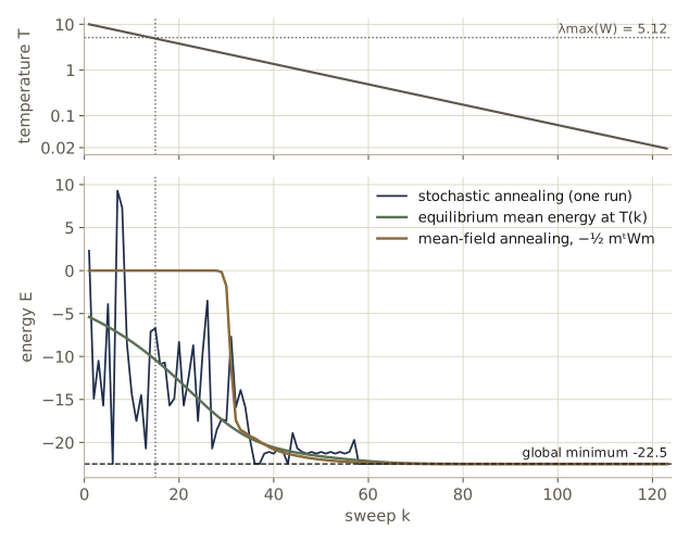
Watch out. Mean-field annealing is an approximation, not a sampler. It ignores the correlations between units, and the configuration it ends in is strongly shaped by the first pattern to emerge at the critical temperature, the top eigenvector of \(\mathbf{W}\). On networks where that pattern points into the wrong basin, deterministic annealing can fail from almost every start while stochastic annealing still succeeds some of the time. Exercise 5 asks you to find such a network.
In large real problems, deterministic annealing is usually much faster than the stochastic version, and the two tend to reach solutions of similar quality. The same machinery applies to other energies — for example, a cubic energy \(-\sum_{ijk} w_{ijk}s_i s_j s_k\) with three-way interactions — but we stay with the quadratic case.
Boltzmann learning
So far the weights were given and we searched for good configurations. Now we turn the question around: can we choose the weights so that the random configurations of the network behave like our data? A network of binary units whose configurations follow the Boltzmann distribution is called a Boltzmann network or Boltzmann machine, and adjusting its weights is Boltzmann learning.
Visible and hidden units
We divide the units into two kinds. Visible units are the ones that receive data: in a classifier, the \(d\) input units hold a binary feature vector and the \(c\) output units hold the category in 1-of-\(c\) form (\(+1\) for the true category, \(-1\) for the others). Hidden units never see data; they give the network extra degrees of freedom. We write \(\alpha\) for a configuration of the visible units and \(\beta\) for a configuration of the hidden units, so a full configuration is the pair \((\alpha, \beta)\) with energy \(E_{\alpha\beta}\). To clamp a unit is to hold it at a fixed value while the others are sampled or annealed.
To classify, we clamp the input units to the feature values, anneal the rest of the network, and read the category from the output units. For that to work, the weights must make the right outputs likely given each input, which is what learning has to achieve.
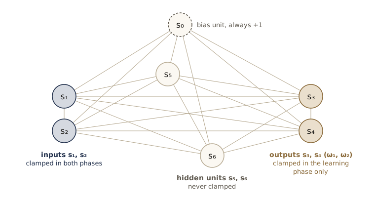
One more ingredient. The energy has no linear terms, so as noted earlier it cannot tell \(\mathbf{s}\) from \(-\mathbf{s}\), and every distribution the network represents would be symmetric under flipping all units. We add a bias unit \(s_0\) that is permanently clamped at \(+1\); its weights \(w_{0i}\) act as thresholds, adding \(-w_{0i}s_i\) to the energy. This is the same trick as the augmented vectors of module 05, and it keeps DHS’s energy formula unchanged. The figure shows the network we will train as a classifier.
Learning the distribution of visible states
Before classification, consider a simpler goal. We are given a desired distribution \(Q(\alpha)\) over visible configurations — in practice, the relative frequencies of the training patterns — and we want the network, running freely at temperature \(T\), to produce visible configurations with probabilities \(P(\alpha)\) close to \(Q(\alpha)\). The network’s probability of a visible configuration sums over the hidden ones:
\[P(\alpha) = \sum_{\beta} P(\alpha, \beta) = \frac{1}{Z}\sum_{\beta} e^{-E_{\alpha\beta}/T}.\]We measure the mismatch with the Kullback–Leibler divergence (relative entropy)
\[D_{\mathrm{KL}}(Q \Vert P) = \sum_{\alpha} Q(\alpha) \ln \frac{Q(\alpha)}{P(\alpha)},\]which is nonnegative and zero exactly when \(P(\alpha) = Q(\alpha)\) for every \(\alpha\). It involves only visible units. Since \(Q\) does not depend on the weights, minimizing it is the same as maximizing \(\sum_\alpha Q(\alpha)\ln P(\alpha)\), the average log-likelihood of the training patterns: Boltzmann learning is maximum-likelihood estimation for this model.
We minimize by gradient descent, \(\Delta w_{ij} = -\eta\, \partial D_{\mathrm{KL}}/\partial w_{ij}\). The derivative is easiest in log form. Write \(\ln P(\alpha) = \ln \sum_\beta e^{-E_{\alpha\beta}/T} - \ln Z\). For \(i \ne j\) the weight \(w_{ij} = w_{ji}\) is a single parameter, and it enters the energy as \(-w_{ij}s_is_j\) (again the two copies cancel the \(\tfrac{1}{2}\)), so \(\partial E/\partial w_{ij} = -s_is_j\). Differentiating a log-sum-exp gives an average:
\[\frac{\partial}{\partial w_{ij}} \ln \sum_\beta e^{-E_{\alpha\beta}/T} = \frac{1}{T}\sum_\beta P(\beta \mid \alpha)\, s_i s_j , \qquad \frac{\partial \ln Z}{\partial w_{ij}} = \frac{1}{T}\sum_{\alpha, \beta} P(\alpha, \beta)\, s_i s_j .\]The first is the correlation of \(s_i\) and \(s_j\) when the visible units are clamped at \(\alpha\) and only the hidden units vary; the second is their correlation when the whole network runs freely. Averaging the first over the training distribution, we define
\[\mathbb{E}_Q[s_is_j]_{\text{clamped}} = \sum_\alpha Q(\alpha) \sum_\beta P(\beta \mid \alpha)\, s_i s_j , \qquad \mathbb{E}[s_is_j]_{\text{free}} = \sum_{\alpha,\beta} P(\alpha, \beta)\, s_is_j ,\]and since \(\partial D_{\mathrm{KL}}/\partial w_{ij} = -\sum_\alpha Q(\alpha)\,\partial \ln P(\alpha)/\partial w_{ij}\), we arrive at the learning rule.
Result (Boltzmann learning). Gradient descent on \(D_{\mathrm{KL}}(Q \Vert P)\) changes each weight by
\[\Delta w_{ij} = \frac{\eta}{T}\Big( \mathbb{E}_Q[s_is_j]_{\text{clamped}} - \mathbb{E}[s_is_j]_{\text{free}} \Big).\]
The first term is called the learning (or teacher) component and the second the unlearning (or student) component. The rule is local — each weight needs only the correlation of the two units it joins, measured in two conditions — and it has a simple reading. If \(s_i\) and \(s_j\) agree more often when the data are imposed than when the network runs on its own, strengthen \(w_{ij}\); if less often, weaken it. The unlearning term removes correlations that the network produces spontaneously but the data do not support. Learning stops when the two correlations match for every pair, a moment-matching condition.
Networks with a handful of units let us compute every term exactly by listing all configurations. The function below arranges the configurations as an array indexed by (visible configuration, hidden configuration, unit), with the bias unit first, and returns the divergence, the two correlation matrices, and \(P(\alpha)\).
def bm_states(n_vis, n_hid):
    """All configurations of a Boltzmann network with a bias unit (index 0, always +1),
    n_vis visible and n_hid hidden units: array of shape (2^n_vis, 2^n_hid, 1 + n_vis + n_hid)."""
    V, H = all_pm1(n_vis), all_pm1(n_hid)
    a, b = len(V), len(H)
    return np.concatenate([np.ones((a, b, 1)),
                           np.repeat(V[:, None, :], b, axis=1),
                           np.repeat(H[None, :, :], a, axis=0)], axis=2)

def bm_exact(W, Q, n_vis, n_hid, T=1.0):
    """Exact D_KL(Q || P), clamped and free correlation matrices, and P(alpha)."""
    S = bm_states(n_vis, n_hid)
    logu = -energy(S, W) / T                                   # log Boltzmann factors, (a, b)
    logP_a = logsumexp(logu, axis=1) - logsumexp(logu)
    P_ab = np.exp(logu - logsumexp(logu))                      # P(alpha, beta)
    P_b_a = np.exp(logu - logsumexp(logu, axis=1, keepdims=True))   # P(beta | alpha)
    free = np.einsum('ab,abi,abj->ij', P_ab, S, S)
    clamped = np.einsum('a,ab,abi,abj->ij', Q, P_b_a, S, S)
    on = Q > 0                                                 # 0 ln 0 = 0
    KL = np.sum(Q[on] * (np.log(Q[on]) - logP_a[on]))
    return KL, clamped, free, np.exp(logP_a)

def random_weights(N_units, rng):
    """Symmetric weights, zero diagonal, uniform on +-sqrt(3/N) (see 'Initialization')."""
    a = np.sqrt(3.0 / N_units)
    U = np.triu(rng.uniform(-a, a, size=(N_units, N_units)), 1)
    return U + U.T
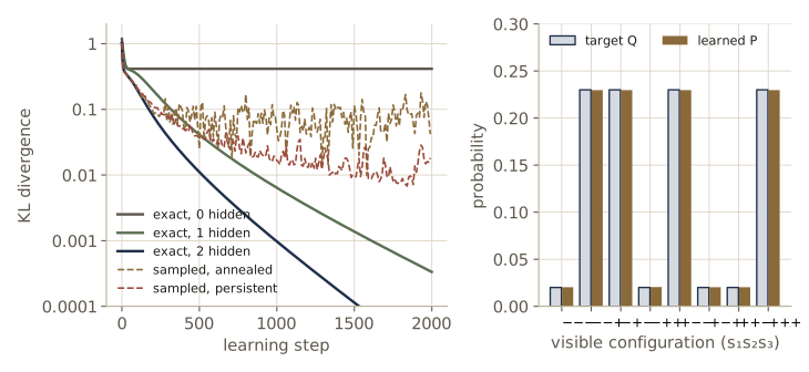
Our target lives on three visible units. It puts probability \(0.23\) on each configuration with an even number of \(-1\) entries (product \(s_1s_2s_3 = +1\)) and \(0.02\) on each of the others: a noisy three-bit parity, in which the third bit is nearly determined by the first two through \(s_3 = s_1s_2\), the \(\pm 1\) form of exclusive-or. First we check the formula against a finite-difference derivative of the divergence.
V3 = all_pm1(3)
Q3 = np.where(V3.prod(axis=1) > 0, 0.23, 0.02)
print("target Q:", Q3, " sum", Q3.sum())

rng_g = np.random.default_rng(1)
Wg = random_weights(6, rng_g)                    # bias + 3 visible + 2 hidden
KL, C, F, _ = bm_exact(Wg, Q3, 3, 2)
h = 1e-6
for i, j in [(0, 2), (1, 3), (3, 5)]:
    Wp = Wg.copy(); Wp[i, j] += h; Wp[j, i] += h
    numeric = (bm_exact(Wp, Q3, 3, 2)[0] - KL) / h
    print(f"dD/dw_{i}{j}: formula {-(C - F)[i, j]:+.6f}   finite difference {numeric:+.6f}")
target Q: [0.02 0.23 0.23 0.02 0.23 0.02 0.02 0.23]  sum 1.0
dD/dw_02: formula -0.421877   finite difference -0.421877
dD/dw_13: formula -0.224823   finite difference -0.224823
dD/dw_35: formula +0.040745   finite difference +0.040745
The formula matches. Now we train networks with zero, one, and two hidden units by exact gradient descent at \(T = 1\) with \(\eta = 0.1\).
def train_visible(Q, n_vis, n_hid, steps=2000, eta=0.1, T=1.0, seed=0):
    """Exact Boltzmann learning of the visible distribution Q."""
    rng_t = np.random.default_rng(seed)
    Wt = random_weights(1 + n_vis + n_hid, rng_t)
    history = []
    for _ in range(steps):
        KL, C, F, P = bm_exact(Wt, Q, n_vis, n_hid, T)
        history.append(KL)
        dW = eta / T * (C - F)                    # the Boltzmann learning rule
        np.fill_diagonal(dW, 0.0)
        Wt += dW
    return Wt, np.array(history), P

kl_hist, W_vis = {}, {}
for n_hid in [0, 1, 2]:
    W_vis[n_hid], kl_hist[n_hid], P_learned = train_visible(Q3, 3, n_hid)
    h_ = kl_hist[n_hid]
    print(f"hidden units {n_hid}: KL at step 0 {h_[0]:.4f}, 100 {h_[100]:.4f}, "
          f"500 {h_[500]:.4f}, 1999 {h_[-1]:.4f}")
print(f"ln 8 - H(Q) = {np.log(8) + np.sum(Q3 * np.log(Q3)):.4f}")
print("learned P (2 hidden):", np.round(P_learned, 4))
hidden units 0: KL at step 0 1.1827, 100 0.4144, 500 0.4144, 1999 0.4144
hidden units 1: KL at step 0 1.0051, 100 0.3417, 500 0.0411, 1999 0.0003
hidden units 2: KL at step 0 1.0198, 100 0.1979, 500 0.0111, 1999 0.0000
ln 8 - H(Q) = 0.4144
learned P (2 hidden): [0.0203 0.2296 0.2296 0.0205 0.2296 0.0203 0.0203 0.2296]
Without hidden units the divergence stalls at \(0.4144\), which equals \(\ln 8 - H(Q)\): the network has learned the uniform distribution. The reason is instructive. With no hidden units, the clamped correlations are just the data correlations \(\mathbb{E}_Q[s_i s_j]\), and for this target every single-unit mean and every pairwise correlation is zero (check a few by hand). The uniform distribution matches all of those moments, so the learning rule has nothing to push against, even though the target is far from uniform. All the structure of parity is in the third-order correlation \(\mathbb{E}_Q[s_1s_2s_3]\), which a network with only pairwise weights cannot represent. One hidden unit is enough to capture it here, and with one or two the divergence heads toward zero. Hidden units are how a Boltzmann machine represents higher-order structure with pairwise weights.
Note. Without hidden units, \(\ln P(\alpha)\) is linear in the weights minus \(\ln Z\), which makes the model an exponential family with the products \(s_is_j\) as sufficient statistics. The divergence is then convex in the weights and Boltzmann learning finds the global optimum (Exercise 7). With hidden units the divergence is no longer convex, and like a multilayer network, the Boltzmann machine can have local optima.
Estimating the correlations by sampling
In a network of realistic size we cannot list the configurations, and the two correlations must be estimated by running the network: clamp the visible units to a training pattern and anneal the hidden units to the learning temperature, then collect \(s_is_j\); do the same with nothing clamped for the free phase. This is stochastic Boltzmann learning. For sampling we use the heat-bath (Gibbs) update: set unit \(i\) to \(+1\) with probability
\[P(s_i = +1 \mid \text{rest}) = \frac{e^{l_i/T}}{e^{l_i/T} + e^{-l_i/T}} = \frac{1}{1 + e^{-2l_i/T}},\]the conditional Boltzmann probability of the unit given its neighbors, derived exactly as the \(\tanh\) formula was. Like the Metropolis rule, it leaves the Boltzmann distribution invariant (Intro to ML, module 11 treats Gibbs sampling in general). Each phase uses 100 parallel chains, a short anneal from \(T = 8\) down to about \(T = 1\), and four sweeps at \(T = 1\) for collecting statistics. The code also has an option we return to below: keeping the free-phase chains running from one weight update to the next instead of restarting them.
def heat_bath_sweep(S, W, free_units, T, rng):
    """One sweep of Gibbs updates over the unclamped units of R chains (rows of S)."""
    for i in rng.permutation(free_units):
        p_plus = expit(2.0 * (S @ W[i]) / T)
        S[:, i] = np.where(rng.random(len(S)) < p_plus, 1.0, -1.0)
    return S

def sampled_correlations(S, W, free_units, schedule, n_collect, rng):
    """Anneal the free units through the schedule, then average s s^t over n_collect sweeps
    at T = 1. Returns the correlations and the final states."""
    for T in schedule:
        S = heat_bath_sweep(S, W, free_units, T, rng)
    corr = np.zeros((S.shape[1], S.shape[1]))
    for _ in range(n_collect):
        S = heat_bath_sweep(S, W, free_units, 1.0, rng)
        corr += S.T @ S / len(S)
    return corr / n_collect, S

def train_visible_stochastic(n_hid, steps=2000, eta=0.1, R=100, seed=0, persistent=False, decay=None):
    """Boltzmann learning of Q3 with sampled correlations. persistent: continue the free-phase
    chains between updates instead of re-annealing; decay: eta_k = eta / (1 + k / decay)."""
    rng_s = np.random.default_rng(seed)
    N_units = 1 + 3 + n_hid
    Ws = random_weights(N_units, rng_s)
    sched = 8.0 * 0.75 ** np.arange(8)                 # 8 -> 1.07
    S_free, history = None, []
    for step in range(steps):
        if step % 10 == 0:
            history.append(bm_exact(Ws, Q3, 3, n_hid)[0])   # exact KL, for monitoring only
        idx = rng_s.choice(len(V3), size=R, p=Q3)           # training patterns drawn from Q
        S = np.column_stack([np.ones(R), V3[idx], rng_s.choice([-1.0, 1.0], size=(R, n_hid))])
        C, _ = sampled_correlations(S, Ws, np.arange(4, N_units), sched, 4, rng_s)       # clamped
        if S_free is None or not persistent:
            S_free = np.column_stack([np.ones(R), rng_s.choice([-1.0, 1.0], size=(R, N_units - 1))])
            F, S_free = sampled_correlations(S_free, Ws, np.arange(1, N_units), sched, 4, rng_s)
        else:
            F, S_free = sampled_correlations(S_free, Ws, np.arange(1, N_units), [], 4, rng_s)
        eta_k = eta if decay is None else eta / (1 + step / decay)
        dW = eta_k * (C - F)
        np.fill_diagonal(dW, 0.0)
        Ws += dW
    return Ws, np.array(history)

W_stoch, kl_stoch = train_visible_stochastic(2)
print("annealed phases, exact KL every 200 steps: ", np.round(kl_stoch[::20], 4))
print(f"  mean over the last 500 steps: {kl_stoch[-50:].mean():.4f}")
W_pers, kl_pers = train_visible_stochastic(2, persistent=True, decay=300)
print("persistent chains, decaying eta:          ", np.round(kl_pers[::20], 4))
print(f"  mean over the last 500 steps: {kl_pers[-50:].mean():.4f}")
annealed phases, exact KL every 200 steps:  [1.0198 0.0933 0.054  0.0905 0.1688 0.0489 0.0474 0.1039 0.0268 0.0998]
  mean over the last 500 steps: 0.0778
persistent chains, decaying eta:           [1.0198 0.1123 0.05   0.031  0.0217 0.0165 0.013  0.0135 0.009  0.0077]
  mean over the last 500 steps: 0.0126
With annealed phases, as DHS describe, the divergence drops quickly at first and then hovers, noisily, well above the exact curve. Two effects are at work. Each update follows a noisy estimate of the gradient, so the weights jitter. More importantly, the estimates are biased: as the weights grow, the network’s distribution develops a few sharp modes, and a short anneal from a random start does not distribute the chains among them in the right proportions, so the free correlations are systematically off. A longer anneal lowers the floor (Exercise 8). A later refinement avoids re-annealing altogether: the free-phase chains simply continue from where they were after the last update, since a small weight change moves the equilibrium only a little. With that change and a learning rate that decreases over time, the sampled version keeps descending, to a divergence several times smaller, and each update is cheaper because the free phase no longer re-anneals.
Learning input–output associations
For classification we do not need the network to model the inputs; we need the right outputs given the inputs. Split the visible configuration into an input part \(\alpha^i\) and an output part \(\alpha^o\). The desired conditional distribution \(Q(\alpha^o \mid \alpha^i)\) comes from the labels, and the criterion is the divergence between conditionals, averaged over inputs:
\[\bar{D}_{\mathrm{KL}} = \sum_{\alpha^i} Q(\alpha^i) \sum_{\alpha^o} Q(\alpha^o \mid \alpha^i) \ln \frac{Q(\alpha^o \mid \alpha^i)}{P(\alpha^o \mid \alpha^i)} .\]The derivation repeats the one above with one change. Now \(\ln P(\alpha^o \mid \alpha^i)\) is the log of a sum over hidden states with inputs and outputs clamped, minus the log of a sum over outputs and hidden states with only the inputs clamped. Each log-sum-exp again differentiates into a correlation, so
\[\Delta w_{ij} = \frac{\eta}{T}\Big( \mathbb{E}_Q[s_is_j]_{\alpha^i \alpha^o\ \text{clamped}} - \mathbb{E}_Q[s_is_j]_{\alpha^i\ \text{clamped}} \Big).\]The inputs are clamped in both phases; only the outputs are released in the unlearning phase. The network never spends effort modeling the distribution of the inputs.
Our classifier is the network in the diagram: inputs \(s_1, s_2\), outputs \(s_3\) (for \(\omega_1\)) and \(s_4\) (for \(\omega_2\)), hidden units \(s_5, s_6\), and the bias \(s_0\). The task is exclusive-or: category \(\omega_1\) when the two inputs agree and \(\omega_2\) when they differ, so the correct output pattern is \((+1, -1)\) or \((-1, +1)\). In code, the configurations are arranged by (input pattern, output pattern, hidden pattern).
X_xor = all_pm1(2)                                    # the four input patterns
labels = (X_xor[:, 0] != X_xor[:, 1]).astype(int)     # 0 = omega_1 (agree), 1 = omega_2 (differ)
O_all = all_pm1(2)                                    # the four output patterns (s3, s4)
target_out = np.where(np.eye(2)[labels] == 1, 1.0, -1.0)
Q_out = np.array([[float(np.all(o == t)) for o in O_all] for t in target_out])   # Q(alpha^o | alpha^i)
Q_in = np.full(4, 0.25)

def bm_conditional(W, n_hid, T=1.0):
    """Exact conditional divergence, learning and unlearning correlations, and P(alpha^o | alpha^i)."""
    S = bm_states(4, n_hid).reshape(4, 4, 2 ** n_hid, -1)          # (input, output, hidden, unit)
    logu = -energy(S, W) / T
    logZ_i = logsumexp(logu, axis=(1, 2))
    logP_o_i = logsumexp(logu, axis=2) - logZ_i[:, None]
    P_ob_i = np.exp(logu - logZ_i[:, None, None])                  # P(alpha^o, beta | alpha^i)
    P_b_io = np.exp(logu - logsumexp(logu, axis=2, keepdims=True)) # P(beta | alpha^i, alpha^o)
    unlearn = np.einsum('i,iob,iobk,iobl->kl', Q_in, P_ob_i, S, S)
    learn = np.einsum('i,io,iob,iobk,iobl->kl', Q_in, Q_out, P_b_io, S, S)
    KL = -np.sum(Q_in[:, None] * Q_out * np.where(Q_out > 0, logP_o_i, 0.0))
    return KL, learn, unlearn, np.exp(logP_o_i)

rng_x = np.random.default_rng(3)
Wx = random_weights(7, rng_x)
KL, Lc, Uc, _ = bm_conditional(Wx, 2)
Wp = Wx.copy(); Wp[1, 4] += 1e-6; Wp[4, 1] += 1e-6
print(f"dD/dw_14: formula {-(Lc - Uc)[1, 4]:+.6f}   finite difference "
      f"{(bm_conditional(Wp, 2)[0] - KL) / 1e-6:+.6f}")
dD/dw_14: formula -0.029306 finite difference -0.029305
It helps to look at the two phases for a single training pattern, as DHS do. Take the input \((s_1, s_2) = (+1, -1)\), whose category is \(\omega_2\), so the outputs are clamped at \((s_3, s_4) = (-1, +1)\) in the learning phase. The cell below computes both correlation matrices for this pattern alone, using the random initial weights, and prints their difference, which is the direction in which the rule moves the weights.
S1 = bm_states(4, 2).reshape(4, 4, 4, -1)[2]          # input pattern (+1, -1): all (output, hidden)
logu = -energy(S1, Wx)
p_free = np.exp(logu - logsumexp(logu))               # outputs and hidden free
o_idx = 1                                             # output pattern (-1, +1)
p_clamp = np.exp(logu[o_idx] - logsumexp(logu[o_idx]))
learn1 = np.einsum('b,bk,bl->kl', p_clamp, S1[o_idx], S1[o_idx])
unlearn1 = np.einsum('ob,obk,obl->kl', p_free, S1, S1)
print("learning minus unlearning correlations (units 0..6 = bias, x1, x2, o1, o2, h1, h2):")
print(np.round(learn1 - unlearn1, 2))
learning minus unlearning correlations (units 0..6 = bias, x1, x2, o1, o2, h1, h2):
[[ 0.    0.    0.   -0.95  1.71  0.77 -0.56]
 [ 0.    0.    0.   -0.95  1.71  0.77 -0.56]
 [ 0.    0.    0.    0.95 -1.71 -0.77  0.56]
 [-0.95 -0.95  0.95  0.   -1.05 -0.61 -0.25]
 [ 1.71  1.71 -1.71 -1.05  0.    0.25  0.68]
 [ 0.77  0.77 -0.77 -0.61  0.25  0.    0.28]
 [-0.56 -0.56  0.56 -0.25  0.68  0.28  0.  ]]
Read the rows of the inputs. The entries between the clamped units — bias, \(s_1\), \(s_2\) — are exactly zero: those units are fixed in both phases, so their correlations are identical and their mutual weights do not move. The entries linking \(s_1 = +1\) to the outputs are negative for \(s_3\) and positive for \(s_4\), and those for \(s_2 = -1\) have the opposite signs. So this pattern pushes \(w_{13}\) down and \(w_{14}\) up, making “\(s_1 = +1\) and \(s_2 = -1\)” favor the output pattern \((-1, +1)\). The hidden units’ rows change too, with mixed signs that depend on the random initial weights: the rule is beginning to recruit them. Averaging such matrices over the four patterns gives the full gradient. We now train the classifier with no hidden units and with two.
def train_conditional(n_hid, steps=1500, eta=0.1, seed=0):
    Wt = random_weights(5 + n_hid, np.random.default_rng(seed))
    history = []
    for _ in range(steps):
        KL, Lc, Uc, P_o_i = bm_conditional(Wt, n_hid)
        history.append(KL)
        dW = eta * (Lc - Uc)
        np.fill_diagonal(dW, 0.0)
        Wt += dW
    return Wt, np.array(history), P_o_i

for n_hid in [0, 2]:
    W_xor, hist_xor, P_o_i = train_conditional(n_hid)
    print(f"hidden units {n_hid}: conditional KL {hist_xor[0]:.4f} -> {hist_xor[-1]:.4f}")
    print("  P(output pattern | input); columns (-,-) (-,+) (+,-) (+,+):")
    for x, row in zip(X_xor.astype(int), P_o_i):
        print(f"  input {x}: {np.round(row, 3)}")
W_xor2 = W_xor
hidden units 0: conditional KL 2.0446 -> 0.6948
  P(output pattern | input); columns (-,-) (-,+) (+,-) (+,+):
  input [-1 -1]: [0.001 0.499 0.499 0.001]
  input [-1  1]: [0.001 0.499 0.499 0.001]
  input [ 1 -1]: [0.001 0.499 0.499 0.001]
  input [1 1]: [0.001 0.499 0.499 0.001]
hidden units 2: conditional KL 1.7754 -> 0.0137
  P(output pattern | input); columns (-,-) (-,+) (+,-) (+,+):
  input [-1 -1]: [0.    0.012 0.987 0.   ]
  input [-1  1]: [0.    0.987 0.012 0.   ]
  input [ 1 -1]: [0.001 0.985 0.013 0.001]
  input [1 1]: [0.001 0.013 0.985 0.001]
With no hidden units the network can do no better than even odds between the two legal outputs for every input — exclusive-or is not linearly separable, the same obstacle a single-layer network meets in module 06. Two hidden units solve it, putting nearly all the probability on the correct output for each input; the illegal output patterns \((-1,-1)\) and \((+1,+1)\) end with negligible probability, although nothing in the rule forbade them explicitly. These conditionals are what the network samples at the learning temperature \(T = 1\) with its inputs clamped. Annealing further toward \(T = 0\) concentrates on the most probable configuration of outputs and hidden units, and since the correct output carries almost all the probability, that configuration has the correct output: the network classifies all four inputs correctly.
Missing features, category constraints, and pattern completion
Because a Boltzmann network models a joint distribution, some problems that are awkward for other classifiers become natural.
Pattern completion. Given part of a pattern, estimate the rest: clamp the known visible units, anneal the others, and read the unknown visible units. The parity network trained above is a small example. The next cell clamps its first two visible units and computes the network’s probability that the third is \(+1\), exactly and by annealing 1000 chains with the heat-bath rule (from \(T = 8\) down to \(T = 1\), then 60 sweeps at \(T = 1\)).
W_par = W_vis[2]
S_par = bm_states(3, 2)                                  # (visible, hidden, unit)
logP_vis = logsumexp(-energy(S_par, W_par), axis=1)      # ln P(alpha) + const
rng_p = np.random.default_rng(4)
sched = np.r_[geometric_schedule(8.0, 0.8, 1.0)[:-1], np.ones(60)]
print("clamped (s1, s2) -> P(s3 = +1): exact   by annealing")
for v12 in all_pm1(2):
    k_minus, k_plus = [np.flatnonzero(np.all(V3 == np.append(v12, s3), axis=1))[0] for s3 in (-1, 1)]
    p_exact = expit(logP_vis[k_plus] - logP_vis[k_minus])
    S = np.column_stack([np.ones(1000), np.tile(v12, (1000, 1)), rng_p.choice([-1.0, 1.0], size=(1000, 3))])
    for T in sched:
        S = heat_bath_sweep(S, W_par, np.array([3, 4, 5]), T, rng_p)
    print(f"  {v12.astype(int)}          {p_exact:.3f}     {np.mean(S[:, 3] > 0):.3f}")
clamped (s1, s2) -> P(s3 = +1): exact   by annealing
  [-1 -1]          0.919     0.919
  [-1  1]          0.082     0.082
  [ 1 -1]          0.081     0.083
  [1 1]          0.919     0.913
Given two bits, the network completes the third according to parity, with the confidence the target assigns (\(0.23/0.25 = 0.92\)), and annealing agrees with the exact answer to within sampling error.
Missing features. If a feature is missing from a pattern, its input unit is left unclamped: during training it acts as a hidden unit for that pattern and settles to values consistent with the rest, and at classification time annealing averages over its possible values. This is the Bayes-correct treatment of a missing feature from module 02 — integrate it out — provided the network’s distribution over the inputs is a sensible one. A network trained with the conditional rule has no reason to model the inputs, since they were clamped in both phases. The cell compares the XOR classifier trained above with a second network of the same shape trained on the joint distribution of inputs and outputs (all four visible units released in the unlearning phase), asking each to classify when the second input is missing.
V4 = all_pm1(4)                                          # visible units (x1, x2, o1, o2)
legal = np.hstack([X_xor, target_out])
Q4 = np.array([0.25 if np.any(np.all(legal == v, axis=1)) else 0.0 for v in V4])
W_joint, _, _ = train_visible(Q4, 4, 2, steps=3000)

for name, Wn in [("conditional training", W_xor2), ("joint training", W_joint)]:
    logu = -energy(bm_states(4, 2).reshape(4, 4, 4, -1), Wn)    # (input, output, hidden)
    P_o_i = np.exp(logsumexp(logu, axis=2) - logsumexp(logu, axis=(1, 2))[:, None])
    p_ok = P_o_i[np.arange(4), [2, 1, 1, 2]]
    print(f"{name}: P(correct output), both inputs known: {np.round(p_ok, 3)}")
    for x1 in [-1.0, 1.0]:
        lu = logu[X_xor[:, 0] == x1]                     # both values of the missing x2
        P_o = np.exp(logsumexp(lu, axis=(0, 2)) - logsumexp(lu))
        print(f"   x1 = {int(x1):+d}, x2 missing: P(omega_1) = {P_o[2]:.3f}, P(omega_2) = {P_o[1]:.3f}")
conditional training: P(correct output), both inputs known: [0.987 0.987 0.985 0.985]
   x1 = -1, x2 missing: P(omega_1) = 0.903, P(omega_2) = 0.096
   x1 = +1, x2 missing: P(omega_1) = 0.518, P(omega_2) = 0.481
joint training: P(correct output), both inputs known: [0.994 0.994 0.991 0.991]
   x1 = -1, x2 missing: P(omega_1) = 0.500, P(omega_2) = 0.500
   x1 = +1, x2 missing: P(omega_1) = 0.500, P(omega_2) = 0.500
Both networks classify complete inputs correctly. With the second input missing, the right answer is an even split, because one input of an exclusive-or says nothing about the category. The jointly trained network gives exactly that. The conditionally trained network does not: with \(x_2\) free, it fills in \(x_2\) from whatever input distribution its weights happen to imply, and for \(x_1 = -1\) that distribution strongly favors one value, so the network confidently picks a category it has no grounds for. Handling missing features well requires modeling the features, which is what the extra cost of joint training buys.
Category constraints. Suppose outside information says that a test pattern is certainly not in categories \(\omega_1\) or \(\omega_4\) of a five-category problem. Clamping those two output units at \(-1\) during the anneal conditions the network on that information, and the category is read from the remaining outputs. In probability terms the network reports its posterior renormalized over the allowed categories; when its probabilities are accurate, using the extra information cannot increase the expected error.
A Boltzmann network with no hidden units and no category units is closely related to the Hopfield network, an associative memory that stores patterns rather than labels. Instead of Boltzmann learning, a Hopfield network sets its weights in one shot to the average correlation of the stored patterns,
\[w_{ij} \propto \mathbb{E}_Q[s_is_j] = \frac{1}{n}\sum_{k=1}^{n} s^{(k)}_i s^{(k)}_j , \qquad w_{ii} = 0 ,\]and recalls by greedy descent (zero temperature) from a partial or noisy pattern. This is fast, but the rule is not the Boltzmann gradient: a network trained this way does not in general satisfy the Boltzmann condition that clamped and free correlations agree. Its capacity is also small. For random patterns of \(d\) bits, reliable recall fails beyond about \(0.14d\) stored patterns. The cell stores \(n\) random 20-bit patterns, hides 6 bits of each, and completes by greedy updates of the hidden bits only.
def hopfield_complete(Pat, known, sweeps=20):
    """Hebbian weights from the stored patterns; complete each pattern from its known bits."""
    Wh = Pat.T @ Pat / len(Pat)
    np.fill_diagonal(Wh, 0.0)
    S = np.where(known, Pat, 0.0)                       # unknown bits start undecided
    unknown = np.flatnonzero(~known)
    for _ in range(sweeps):
        for i in unknown:
            l = S @ Wh[i]
            S[:, i] = np.where(l >= 0, 1.0, -1.0)
    return S

rng_h = np.random.default_rng(5)
d_h = 20
known = np.ones(d_h, dtype=bool)
known[rng_h.choice(d_h, 6, replace=False)] = False
for n_pat in [2, 3, 5, 8]:
    Pat = rng_h.choice([-1.0, 1.0], size=(n_pat, d_h))
    done = hopfield_complete(Pat, known)
    ok = np.all(done == Pat, axis=1)
    print(f"{n_pat} stored patterns (0.14 d = {0.14 * d_h:.1f}): {ok.sum()} of {n_pat} completed exactly")
2 stored patterns (0.14 d = 2.8): 2 of 2 completed exactly
3 stored patterns (0.14 d = 2.8): 3 of 3 completed exactly
5 stored patterns (0.14 d = 2.8): 4 of 5 completed exactly
8 stored patterns (0.14 d = 2.8): 3 of 8 completed exactly
Two and three stored patterns are completed perfectly (the \(0.14d\) limit is a statistical statement about large networks, not a sharp threshold); with five, one completion fails, and with eight, most do, because the stored patterns interfere with one another. A Boltzmann network with hidden units can store more by adding hidden units, at the price of real Boltzmann learning.
Deterministic Boltzmann learning
Stochastic Boltzmann learning is expensive: every weight update needs two anneals per training pattern, each with many sweeps. Just as mean-field annealing replaces stochastic annealing, deterministic Boltzmann learning replaces both phases with mean-field annealing and approximates each correlation by a product of averages,
\[\mathbb{E}[s_is_j] \approx \mathbb{E}[s_i]\,\mathbb{E}[s_j] \approx m_i m_j .\]DHS Algorithm 3 runs as follows, for a training set \(\mathcal{D}\) of patterns with features and categories:
- Pick a training pattern at random.
- Clamp its inputs and outputs, start the hidden units at small random values, and run mean-field annealing down to the learning temperature. Record the products \(m_im_j\).
- Clamp only the inputs, restart the outputs and hidden units, and anneal again. Record \(m_im_j\).
- Update \(w_{ij} \leftarrow w_{ij} + \frac{\eta}{T}\big( [m_im_j]_{\text{inputs, outputs clamped}} - [m_im_j]_{\text{inputs clamped}} \big)\), and repeat until the weights stop changing.
We train the XOR network this way from four different random starts, anneal each phase from \(T = 5\) down to \(T = 1\), and judge the results two ways: by the exact probabilities of the stochastic network with the learned weights, and by what the mean-field network itself outputs.
def mf_settle(m, W, free_units, schedule, rng):
    """Mean-field annealing of one network state m (1-D), only the free units updated."""
    m = m.copy()
    for T in schedule:
        for i in rng.permutation(free_units):
            m[i] = np.tanh(W[i] @ m / T)
    return m

def train_deterministic(n_hid, epochs=300, eta=0.05, seed=0):
    rng_d = np.random.default_rng(seed)
    N_units = 5 + n_hid
    Wd = random_weights(N_units, rng_d)
    sched = np.concatenate([5.0 * 0.7 ** np.arange(5), [1.0, 1.0, 1.0]])
    for _ in range(epochs):
        for p in rng_d.permutation(4):
            m = np.concatenate([[1.0], X_xor[p], target_out[p], rng_d.uniform(-0.1, 0.1, n_hid)])
            m_clamped = mf_settle(m, Wd, np.arange(5, N_units), sched, rng_d)
            m = np.concatenate([[1.0], X_xor[p], rng_d.uniform(-0.1, 0.1, 2 + n_hid)])
            m_free = mf_settle(m, Wd, np.arange(3, N_units), sched, rng_d)
            dW = eta / sched[-1] * (np.outer(m_clamped, m_clamped) - np.outer(m_free, m_free))
            np.fill_diagonal(dW, 0.0)
            Wd += dW
    return Wd, sched

for seed in range(4):
    Wd, sched = train_deterministic(2, seed=seed)
    KL, _, _, P_o_i = bm_conditional(Wd, 2)
    rng_e = np.random.default_rng(9)
    outs = np.array([mf_settle(np.concatenate([[1.0], x, rng_e.uniform(-0.1, 0.1, 4)]), Wd,
                               np.arange(3, 7), sched, rng_e)[3:5] for x in X_xor])
    mf_correct = np.all(np.sign(outs) == target_out, axis=1).sum()
    p_correct = P_o_i[np.arange(4), [2, 1, 1, 2]]
    print(f"start {seed}: mean-field outputs correct for {mf_correct}/4 inputs;"
          f"  exact P(correct output) = {np.round(p_correct, 2)}")
start 0: mean-field outputs correct for 4/4 inputs;  exact P(correct output) = [0.92 0.98 0.78 0.78]
start 1: mean-field outputs correct for 4/4 inputs;  exact P(correct output) = [0.87 0.81 0.82 0.48]
start 2: mean-field outputs correct for 4/4 inputs;  exact P(correct output) = [0.81 0.65 0.91 0.96]
start 3: mean-field outputs correct for 4/4 inputs;  exact P(correct output) = [0.77 0.95 0.8  0.73]
The mean-field network classifies all four inputs correctly from every start. The stochastic network with the same weights is less sure of itself: its exact probability of the correct output ranges from about 0.5 to above 0.9, below what exact gradient descent achieved earlier. The mean-field approximation drops the fluctuations that the true correlations include, so the weights it learns are tuned to the deterministic network that produced them. When the network will be used deterministically, that is exactly what we want, and it is much cheaper; the approximation is known to go wrong in some cases, and DHS note that these are rare in practice.
Initialization and setting parameters
A Boltzmann network has several interacting settings. DHS give rules of thumb for each.
Topology and hidden units. The number of visible units is fixed by the number of binary features and categories, and in the absence of other knowledge the network is fully connected, so the main choice is the number of hidden units. A common simplification removes the connections within the input group and within the output group; it trains faster but handles pattern completion and missing features less well. Two bounds bracket the number of hidden units for a training set of \(n\) distinct patterns. At most \(n\) are needed: one hidden unit per training pattern, wired to switch on only for its pattern and to excite that pattern’s category, stores the training set in the manner of the probabilistic neural network of module 04 — and generalizes about as poorly as that suggests. At least \(\lceil \log_2 n \rceil\) are needed if every pattern is to get its own hidden configuration. Between those bounds the right number depends on the problem; the usual practice is to start with a generous network and use weight decay, shrinking every weight slightly toward zero at each step with a decay rate that decreases over training, so that weights supported only by chance correlations fade away. Averaging over states smooths the decision boundaries, so a Boltzmann network suffers less from too many hidden units than a backpropagation network does.
Initial weights. Zero weights work but learn slowly, and with fully connected hidden units there is nothing to tell them apart. Random weights of both signs break the symmetry. The scale follows from asking the local field on each unit to have variance about 1 at the start, the range where \(\tanh(l/T)\) at \(T = 1\) is neither flat nor saturated. If each unit is \(\pm 1\) with equal probability and the \(N - 1\) incoming weights are independent and uniform on \([-a, a]\), each term \(w_{ij}s_j\) has mean zero and variance \(\mathbb{E}[w_{ij}^2] = a^2/3\), so
\[\operatorname{Var}(l_i) = (N-1)\frac{a^2}{3} = 1 \quad\Longrightarrow\quad a = \sqrt{\frac{3}{N-1}} \approx \sqrt{\frac{3}{N}} .\]Our random_weights uses \(a = \sqrt{3/N}\).
Initial temperature. \(T(1)\) should be just high enough that nearly all proposed moves are accepted; higher only wastes sweeps. DHS describe an empirical procedure. In a short run of trial polls at temperature \(T\), let \(m_1\) be the number of proposals that lower the energy (always accepted), \(m_2\) the number that raise it, and \(\Delta E^{+}\) the average increase over the latter. If the uphill ones are accepted with probability about \(e^{-\Delta E^{+}/T}\), the acceptance ratio is
\[R = \frac{m_1 + m_2\, e^{-\Delta E^{+}/T}}{m_1 + m_2} .\]Solving for the temperature that gives a desired ratio \(R\),
\[T = \frac{\Delta E^{+}}{\ln m_2 - \ln\!\big(m_2 R - m_1(1 - R)\big)} .\]The statistics depend on the temperature at which they were gathered, so we alternate: run trial polls at the current \(T\), recompute \(T\) from the formula, and repeat until it settles. The cell checks the weight scale on a 20-unit network and then applies the temperature procedure to our 12-unit network with target \(R = 0.9\).
N_big = 20
W_big = random_weights(N_big, np.random.default_rng(6))
S_rand = np.random.default_rng(7).choice([-1.0, 1.0], size=(5000, N_big))
print(f"variance of local fields at random states: {np.var(S_rand @ W_big):.3f}  "
      f"(target 1; exact for this matrix: {np.sum(W_big ** 2) / N_big:.3f})")

def initial_temperature(W, R_target, T, rounds, polls, rng):
    """Iterate DHS's acceptance-ratio formula for T(1)."""
    S = rng.choice([-1.0, 1.0], size=(1, W.shape[0]))
    for r in range(rounds):
        dEs, accepted = [], 0
        for _ in range(polls):
            i = rng.integers(W.shape[0])
            dE = 2 * S[0, i] * (S[0] @ W[i])
            dEs.append(dE)
            if dE <= 0 or rng.random() < np.exp(-dE / T):
                S[0, i] *= -1
                accepted += 1
        dEs = np.array(dEs)
        m1, m2 = np.sum(dEs <= 0), np.sum(dEs > 0)
        dE_plus = dEs[dEs > 0].mean()
        print(f"round {r}: T = {T:6.2f}, observed acceptance {accepted / polls:.3f}, "
              f"m1 = {m1}, m2 = {m2}, mean uphill dE = {dE_plus:.2f}")
        T = dE_plus / (np.log(m2) - np.log(m2 * R_target - m1 * (1 - R_target)))
    return T

T1 = initial_temperature(W, 0.9, 1.0, 5, 2000, np.random.default_rng(8))
print(f"suggested T(1) = {T1:.2f}")
variance of local fields at random states: 1.015  (target 1; exact for this matrix: 1.013)
round 0: T =   1.00, observed acceptance 0.097, m1 = 105, m2 = 1895, mean uphill dE = 7.43
round 1: T =  66.58, observed acceptance 0.960, m1 = 970, m2 = 1030, mean uphill dE = 5.01
round 2: T =  23.23, observed acceptance 0.894, m1 = 891, m2 = 1109, mean uphill dE = 5.07
round 3: T =  25.52, observed acceptance 0.910, m1 = 932, m2 = 1068, mean uphill dE = 5.08
round 4: T =  24.50, observed acceptance 0.893, m1 = 918, m2 = 1082, mean uphill dE = 5.42
suggested T(1) = 26.50
The field variance comes out close to 1, as designed. The temperature procedure jumps from a poor first guess to the right range after one round and then fluctuates around 25, where about nine proposals in ten are accepted. That is higher than the \(T(1) = 10\) we used earlier. Since the critical temperature of this network is about 5, our earlier choice was already high enough for the search to start from effectively random states, and starting at 25 would add sweeps without changing the outcome; the acceptance-ratio rule is a safe default, not a minimum.
Learning rate. The divergence is a smooth function of the weights, and as with backpropagation in module 06, its curvature limits the stable step size. Under mild assumptions DHS derive (Problem 18) the bound \(\eta < T^2/N\) for a fully connected network of \(N\) units: larger temperatures smooth the error surface and allow larger steps. Our runs at \(T = 1\) with \(N \le 7\) units use \(\eta \le 0.1\), inside this bound.
Other heuristics and stopping. Early in an anneal it can pay to propose flipping several units at once, finishing with single-unit polls; and it often pays to remember the best configuration seen, as we did. There are two stopping rules. A single anneal stops when the temperature is so low that no uphill moves are accepted; a final sweep of single-unit polls then confirms a local minimum. Training as a whole stops when the error on a validation set (module 09) stops improving; overfitting tends to be milder than in multilayer networks, again because of the averaging over states.
Boltzmann networks and graphical models
The learning rule never used the fact that the network was fully connected. It applies unchanged to any topology — missing links are weights fixed at zero — and it is easy to add constraints such as weight sharing, where several links must carry the same value: we simply add up the updates of all links in a shared group and apply the sum to each. Structured Boltzmann networks of this kind can mimic other probabilistic models, giving new ways to train them.
The cleanest example is the hidden Markov model of module 03 (and Intro to ML, module 13). An HMM with \(c\) hidden states and transition probabilities \(a_{ij} = P(\omega_j(t+1) \mid \omega_i(t))\) emits a visible symbol \(v_k\) at each step with probability \(b_{jk} = P(v_k(t) \mid \omega_j(t))\). Unfold it in time into its trellis and put one binary unit at each node: at each time \(t = 1, \dots, T_f\) a group of \(c\) hidden units and a group of visible units, one per symbol. (We write \(T_f\) for the sequence length to keep \(T\) for temperature.) It is simplest to let these units take values 0 and 1, and to allow only legal configurations, in which exactly one unit in each group is on. Link hidden unit \(i\) at time \(t-1\) to hidden unit \(j\) at time \(t\) with weight \(A_{ij}\), the same at every \(t\) (weight sharing), and hidden unit \(j\) to visible unit \(k\) at the same time with weight \(B_{jk}\). With 0/1 units only links between two active units contribute, so a legal configuration — a hidden path \(\omega(1), \dots, \omega(T_f)\) with the observed symbols \(v(1), \dots, v(T_f)\) — has energy
\[E = -\sum_{t=1}^{T_f} A_{\omega(t-1)\,\omega(t)} - \sum_{t=1}^{T_f} B_{\omega(t)\, v(t)} .\]This network is called a Boltzmann chain. If we set
\[A_{ij} = T \ln a_{ij}, \qquad B_{jk} = T \ln b_{jk},\]then \(e^{-E/T} = \prod_t a_{\omega(t-1)\omega(t)}\, b_{\omega(t)v(t)}\), exactly the HMM’s joint probability of the path and the sequence (with the initial hidden state \(\omega(0)\) known). Summing the Boltzmann factors over all legal hidden paths with the visible units clamped therefore gives \(P(\mathbf{V}^{T_f})\), the quantity the forward algorithm computes, and the Boltzmann distribution over paths is the HMM’s posterior over hidden paths. The cell checks this for a two-state, three-symbol model at an arbitrary temperature.
a = np.array([[0.7, 0.3], [0.4, 0.6]])                 # transition probabilities a_ij
b = np.array([[0.5, 0.4, 0.1], [0.1, 0.3, 0.6]])       # emission probabilities b_jk
v_seq = [0, 2, 1, 2]                                   # observed symbols
omega0, T_chain = 0, 1.7                               # known initial state; any temperature
A_w, B_w = T_chain * np.log(a), T_chain * np.log(b)    # Boltzmann chain weights

alpha = np.eye(2)[omega0]                              # forward algorithm
for v in v_seq:
    alpha = (alpha @ a) * b[:, v]
Z_chain, best_path, best_E = 0.0, None, np.inf
for path in itertools.product([0, 1], repeat=len(v_seq)):     # all legal hidden configurations
    prev = (omega0,) + path[:-1]
    E = -sum(A_w[i, j] for i, j in zip(prev, path)) - sum(B_w[j, v] for j, v in zip(path, v_seq))
    Z_chain += np.exp(-E / T_chain)
    if E < best_E:
        best_E, best_path = E, path
print(f"forward algorithm P(V) = {alpha.sum():.6f}")
print(f"Boltzmann chain, sum of exp(-E/T) over legal paths = {Z_chain:.6f}")
print(f"lowest-energy hidden path {best_path} (the most probable path)")
forward algorithm P(V) = 0.010990
Boltzmann chain, sum of exp(-E/T) over legal paths = 0.010990
lowest-energy hidden path (0, 1, 1, 1) (the most probable path)
The two numbers agree, and the lowest-energy configuration is the most probable hidden path, the one the Viterbi algorithm would find. Training the chain with Boltzmann learning, with the visible units clamped to training sequences and the weight-sharing constraint in force, is an alternative to Baum–Welch. Once the constrained network is trained this way, however, its weights need not map back to proper probabilities through \(A_{ij} = T\ln a_{ij}\), because nothing forces the corresponding \(a_{ij}\) to sum to one.
Other graphical models
The same correspondence extends to Bayesian belief networks, directed acyclic graphs of discrete variables linked by conditional probabilities (Intro to ML, module 08). It is clearest when every variable is binary; for variables with several values, groups of units with a one-active-unit constraint play the role of each variable, as the hidden groups did in the chain.
Structured Boltzmann networks shine where the classical algorithms struggle. A signal with two time scales — rapid fluctuations riding on slow trends — calls for two coupled hidden Markov chains, but coupling them creates loops, and the forward–backward algorithm no longer applies exactly. Two Boltzmann chains with cross-connections between their hidden units, a structure DHS call a Boltzmann zipper, can be trained with the same learning rule: one chain sampled quickly picks up short-range structure, the other sampled slowly picks up long-range structure, and the cross-weights learn how the two relate. Speech is the standard motivation, with fast phonetic transitions superimposed on slower prosody.
Note. A later, influential descendant is the restricted Boltzmann machine, a two-layer network with visible–hidden connections only. With no connections within a layer, the hidden units are conditionally independent given the visible ones and vice versa, so the clamped phase needs no sampling at all and the free phase can be sampled layer by layer. The two-layer variant is mentioned by DHS under the name harmonium.
Evolutionary methods
The second family of stochastic methods is modeled on biological evolution. Instead of improving one candidate, we keep a population of candidate classifiers, each a little different from the others. We score each one on the task — for example, its accuracy on a set of labeled samples — and, in keeping with the biological analogy, call the score its fitness. The fitter candidates are kept and used as parents; random alterations of the parents produce the offspring that make up the next generation. Some offspring are better than their parents and some are worse, but because selection favors fit parents, the population improves on average from one generation to the next. The process stops when the best candidate reaches a desired fitness \(\theta\) or a budget runs out.
Two features distinguish this from the searches earlier in the module. The candidates evaluate independently, so the method parallelizes naturally. And the random alterations sometimes make large jumps, so the search can move across discontinuous, rugged landscapes where no gradient exists. How candidates are represented determines what alterations are possible: bit strings in genetic algorithms, pieces of program in genetic programming.
Genetic algorithms
In a basic genetic algorithm each candidate is a string of bits called a chromosome, and the designer decides how the bits map to a classifier. Three genetic operators produce offspring:
- Replication: copy a chromosome unchanged.
- Crossover: pick a random split point, and exchange the tails of two parent chromosomes, producing two offspring that each combine a head from one parent and a tail from the other. A pair of parents undergoes crossover with probability \(P_{\text{co}}\).
- Mutation: flip each bit independently with a small probability \(P_{\text{mut}}\).
Other operators are possible — inversion, reversing a chromosome, is one — but rarely useful, since reversing a good chromosome almost always destroys what made it good.
Representation. The mapping from bits to classifier is where domain knowledge enters. The simplest mapping lets each bit switch one feature on or off, which is the representation we use. Others encode the weights of a network with a fixed topology in segments of bits, let bits say which pairs of units are connected, or encode a decision tree: a block of bits per node giving a sign, which feature to test, and a threshold, as with the trees of module 08. A good representation keeps functionally related bits close together, because crossover rarely separates neighbors; then one parent’s good block for one part of the problem can be joined with another parent’s good block for another part.
Scoring. For \(c\) categories it is usually easiest to evolve \(c\) dichotomizers, each separating one category from the rest. The goal is accuracy on future patterns (or low expected cost), so the score is typically accuracy on a labeled set, but a search that evaluates thousands of candidates on the same data can tune itself to that data’s accidents — overfitting in a new guise. Penalizing complexity in the score and limiting the search are the usual defenses.
Selection. DHS’s basic algorithm ranks the chromosomes and breeds from the top of the ranking (truncation or rank selection). An alternative is fitness-proportional selection, in which chromosome \(i\) is chosen as a parent with probability \(f_i/\sum_k f_k\); weaker chromosomes are sometimes chosen, which preserves diversity. A generalization weights by an increasing function of fitness, and a choice modeled on the Boltzmann factor is
\[P(i) = \frac{e^{f_i/T}}{\sum_{k} e^{f_k/T}},\]with a temperature \(T\) that starts high (almost uniform selection, broad exploration) and can be lowered to concentrate on the fittest (exploitation).
Our task is feature selection. We have \(d = 16\) features for a two-category problem: features 0–3 are informative, features 4–7 are noisy copies of them, and features 8–15 are pure noise. The classifier is the minimum-distance (nearest class mean) rule from module 02, which is optimal for spherical Gaussian classes with equal priors but is hurt by irrelevant features, since they add noise to every distance. A chromosome is a 16-bit mask saying which features the classifier uses. Its fitness is accuracy on a validation set minus a small penalty of \(0.005\) per feature used. With only \(2^{16} - 1 = 65{,}535\) nonempty masks we can score them all and know the true optimum.
d = 16
def make_features(n_per_class, rng):
    """Two classes; features 0-3 informative, 4-7 noisy copies of them, 8-15 noise."""
    y = np.repeat([0, 1], n_per_class)
    mu = np.full(4, 1.2)
    Z = rng.normal(0.0, 1.0, (2 * n_per_class, 4)) + np.where(y[:, None] == 1, mu / 2, -mu / 2)
    copies = Z + rng.normal(0.0, 1.0, Z.shape)
    noise = rng.normal(0.0, 1.0, (2 * n_per_class, 8))
    return np.hstack([Z, copies, noise]), y

rng_d = np.random.default_rng(8)
X_tr, y_tr = make_features(50, rng_d)        # training set: class means
X_va, y_va = make_features(100, rng_d)       # validation set: fitness
X_te, y_te = make_features(2000, rng_d)      # test set: judged only at the end
m0, m1 = X_tr[y_tr == 0].mean(axis=0), X_tr[y_tr == 1].mean(axis=0)

def accuracy(masks, X, y):
    """Nearest-mean accuracy of each feature mask (rows of masks) on (X, y)."""
    masks = np.atleast_2d(masks)
    d0 = ((X - m0) ** 2) @ masks.T            # squared distances using only the masked features
    d1 = ((X - m1) ** 2) @ masks.T
    return ((d1 < d0).astype(int) == y[:, None]).mean(axis=0)

def fitness(masks, penalty=0.005):
    masks = np.atleast_2d(masks)
    return accuracy(masks, X_va, y_va) - penalty * masks.sum(axis=1)

all_masks = np.array(list(itertools.product([0, 1], repeat=d)))[1:]
f_all = fitness(all_masks)
f_opt = f_all.max()
best_mask = all_masks[np.argmax(f_all)]
print(f"best of all {len(all_masks)} masks: fitness {f_opt:.3f}, features {np.flatnonzero(best_mask)}")
print(f"masks within 0.01 of the best (counting the best): {np.sum(f_all > f_opt - 0.01)}")
print(f"all 16 features: fitness {fitness(np.ones(d))[0]:.3f};  features 0-3 only: "
      f"{fitness(np.r_[np.ones(4), np.zeros(12)])[0]:.3f}")
best of all 65535 masks: fitness 0.870, features [ 0  1  2  3  5 13]
masks within 0.01 of the best (counting the best): 2
all 16 features: fitness 0.735;  features 0-3 only: 0.850
The best mask uses the four informative features plus one noisy copy (feature 5) and one pure-noise feature (13); the noise feature earns its place only by happening to help on these 200 validation samples, a first sign of the overfitting risk. The top of the landscape is a narrow peak: only one other mask scores within 0.01 of the best. Now the genetic algorithm. Each generation keeps the single best chromosome unchanged (elitism, a form of replication), then fills the population by choosing parent pairs, crossing them over with probability \(P_{\text{co}}\), and mutating each offspring.
def genetic_algorithm(fitness, n_bits, L=30, generations=40, p_co=0.8, p_mut=None,
                      selection="rank", T_sel=0.01, seed=0):
    """Basic GA with elitism. selection: 'rank' (breed from the top half), 'proportional',
    or 'boltzmann' (P(i) proportional to exp(f_i / T_sel)). Returns the final population
    and the best and mean fitness of every generation."""
    rng_ga = np.random.default_rng(seed)
    p_mut = 1.0 / n_bits if p_mut is None else p_mut
    pop = rng_ga.integers(0, 2, size=(L, n_bits))
    best, mean, pops = [], [], []
    for g in range(generations + 1):
        f = fitness(pop)
        best.append(f.max()); mean.append(f.mean()); pops.append(pop)
        if g == generations:
            break
        order = np.argsort(-f)
        if selection == "rank":
            pool, probs = order[: L // 2], None
        elif selection == "proportional":
            pool, probs = np.arange(L), f / f.sum()
        else:
            w = np.exp((f - f.max()) / T_sel)
            pool, probs = np.arange(L), w / w.sum()
        children = [pop[order[0]].copy()]                     # elitism
        while len(children) < L:
            pa, pb = pop[rng_ga.choice(pool, size=2, p=probs)]
            if rng_ga.random() < p_co:                        # one-point crossover
                cut = rng_ga.integers(1, n_bits)
                kids = [np.r_[pa[:cut], pb[cut:]], np.r_[pb[:cut], pa[cut:]]]
            else:
                kids = [pa.copy(), pb.copy()]
            for k in kids:
                flip = rng_ga.random(n_bits) < p_mut          # mutation
                k[flip] = 1 - k[flip]
                if len(children) < L:
                    children.append(k)
        pop = np.array(children)
    return pop, np.array(best), np.array(mean), pops

pop, ga_best, ga_mean, ga_pops = genetic_algorithm(fitness, d, seed=0)
for g in [0, 5, 10, 20, 40]:
    print(f"generation {g:2d}: best {ga_best[g]:.3f}   mean {ga_mean[g]:.3f}")
winner = pop[np.argmax(fitness(pop))]
print(f"final best features {np.flatnonzero(winner)}; global optimum first reached in generation "
      f"{np.argmax(np.isclose(ga_best, f_opt))}")
print(f"fitness evaluations used: {30 * 41} of {len(all_masks)} possible masks")
generation  0: best 0.830   mean 0.751
generation  5: best 0.845   mean 0.813
generation 10: best 0.855   mean 0.821
generation 20: best 0.865   mean 0.838
generation 40: best 0.870   mean 0.837
final best features [ 0  1  2  3  5 13]; global optimum first reached in generation 30
fitness evaluations used: 1230 of 65535 possible masks
The best fitness climbs in steps, and the population reaches the global optimum after 30 generations, having evaluated under 2% of the masks. Is that luck, and does the selection scheme matter? The next cell repeats the run with 20 different seeds for each scheme and compares with pure random search using the same number of evaluations.
print("selection               reached optimum   mean final best")
for name, kw in [("rank (top half)", dict(selection="rank")),
                 ("fitness-proportional", dict(selection="proportional")),
                 ("Boltzmann, T = 0.02", dict(selection="boltzmann", T_sel=0.02)),
                 ("Boltzmann, T = 0.01", dict(selection="boltzmann", T_sel=0.01))]:
    finals = np.array([genetic_algorithm(fitness, d, seed=s, **kw)[1][-1] for s in range(20)])
    print(f"{name:22s}   {np.mean(np.isclose(finals, f_opt)):14.0%}   {finals.mean():15.4f}")
rng_r = np.random.default_rng(0)
finals = np.array([fitness(rng_r.integers(0, 2, size=(30 * 41, d))).max() for _ in range(20)])
print(f"{'random search':22s}   {np.mean(np.isclose(finals, f_opt)):14.0%}   {finals.mean():15.4f}")
f0 = fitness(ga_pops[0])
print(f"generation 0 of the first run: fitness from {f0.min():.3f} to {f0.max():.3f}; under proportional "
      f"selection the best is only {f0.max() / f0.min():.2f} times as likely to be picked as the worst")
selection               reached optimum   mean final best
rank (top half)                     90%            0.8688
fitness-proportional                30%            0.8595
Boltzmann, T = 0.02                 90%            0.8688
Boltzmann, T = 0.01                 80%            0.8665
random search                        0%            0.8500
generation 0 of the first run: fitness from 0.625 to 0.830; under proportional selection the best is only 1.33 times as likely to be picked as the worst
Rank selection and Boltzmann selection find the optimum in most runs; random search with the same budget never does. Fitness-proportional selection does poorly here, and the reason is worth remembering: the fitness values are all positive and close together, so the fittest chromosome is chosen barely more often than the weakest (the last line of the output says by how much), and selection exerts almost no pressure. Rank selection and the Boltzmann weights depend on differences in fitness, not ratios, so they are unaffected by the offset.
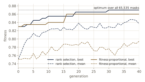
The winning mask was chosen on the validation set; the test set tells us how it generalizes.
for name, mask in [("GA winner", winner), ("features 0-3", np.r_[np.ones(4), np.zeros(12)]),
                   ("all 16 features", np.ones(d))]:
    print(f"{name:16s} test accuracy {accuracy(mask, X_te, y_te)[0]:.4f}")
GA winner        test accuracy 0.8822
features 0-3     test accuracy 0.8850
all 16 features  test accuracy 0.8665
The selected subset beats using all features, but the four informative features alone do slightly better on new data: the extra noise feature was an artifact of the validation set. The genetic algorithm did its job — it optimized the score it was given — and the lesson is about the score. Searching over many candidates with one validation set overfits that set, which is why the final evaluation needs data the search never saw (module 09).
Further heuristics
Genetic algorithms invite endless variations; a few recur.
- Adapting the rates. If \(P_{\text{co}}\) and \(P_{\text{mut}}\) are too small, the population improves slowly; if they are too large, offspring have little in common with their parents and the search degenerates into random sampling. The rates can be adjusted by monitoring the improvement per generation, or encoded in the chromosomes themselves so that evolution tunes them.
- Non-binary alphabets. Chromosomes over three or more symbols bring little algorithmic advantage but can make the mapping to a classifier more natural, for example a ternary chromosome for a tree with three-way splits.
- Variable length. When longer chromosomes describe larger classifiers (more hidden units, say), an insertion operator that splices new bits into a random position lets the size evolve. Such “messy” genetic algorithms are a step toward genetic programming.
Why do they work?
With so many interacting choices — population size, rates, representation, selection, the difficulty of the problem — there are few firm theorems about genetic algorithms. Replication plus mutation alone is essentially a parallel random local search. Crossover is what makes the method different, and the classical argument for it is Holland’s schema idea.
A schema is a template over \(\{0, 1, *\}\), where \(*\) matches either bit; for example, 1111************ describes every chromosome that uses features 0–3. Its order \(o(H)\) is the number of fixed positions (4 here) and its defining length \(\delta(H)\) is the distance between the first and last fixed positions (3 here). For fitness-proportional selection, one-point crossover, and bitwise mutation, one can bound the expected number of chromosomes matching schema \(H\) in the next generation:
where \(f(H)\) is the average fitness of the matching chromosomes and \(\bar{f}\) the population average. Selection multiplies the count by \(f(H)/\bar{f}\); crossover can destroy the schema only by cutting between its fixed positions, with probability at most \(\delta(H)/(d-1)\); mutation destroys it only by hitting one of its \(o(H)\) fixed bits. So short, low-order schemata with above-average fitness — building blocks — tend to multiply, and crossover assembles them into complete solutions. The argument is only a lower bound on an expectation, and it says nothing about whether building blocks combine well. But it makes a useful design point concrete: the representation should put bits that work together close to one another. We can watch our schema spread in the rank-selection run above.
schema = np.r_[np.ones(4, dtype=int), -np.ones(12, dtype=int)]      # 1111************
fixed = schema >= 0
for g in [0, 2, 4, 6, 8, 10, 20]:
    frac = np.mean(np.all(ga_pops[g][:, fixed] == schema[fixed], axis=1))
    print(f"generation {g:2d}: fraction of population matching 1111************ = {frac:.2f}")
generation  0: fraction of population matching 1111************ = 0.07
generation  2: fraction of population matching 1111************ = 0.20
generation  4: fraction of population matching 1111************ = 0.13
generation  6: fraction of population matching 1111************ = 0.17
generation  8: fraction of population matching 1111************ = 0.33
generation 10: fraction of population matching 1111************ = 0.53
generation 20: fraction of population matching 1111************ = 0.83
In generation 0 the schema is matched about as often as chance predicts (\(1/16 \approx 0.06\)); selection and crossover spread it to half the population by generation 10 and to most of it by generation 20. In our problem the four informative features happen to be adjacent, so this schema has a short defining length and survives crossover well; Exercise 11 asks what happens when they are scattered.
Genetic programming
Genetic programming keeps the population-and-selection loop of a genetic algorithm but changes the representation: each candidate is a small computer program, typically an arithmetic or logical expression built from operators, variables, and constants. Lisp-style prefix expressions such as (+ x 2) and (* 3 (+ y 5)) are convenient because every expression is an operator followed by its operands, which may themselves be expressions — that is, a tree with operators at the internal nodes and variables and constants at the leaves. We represent such trees in Python as nested tuples, ('*', 3.0, ('+', 'y', 5.0)).
The operators act on trees:
- Replication: copy a program unchanged.
- Crossover: choose a random node in each of two parents and swap the subtrees rooted there. Any subtree is a well-formed expression, so the offspring are well formed too.
- Mutation: give each node a small chance of being replaced by an element of the same kind — a binary operator by another binary operator, a leaf by another variable or constant — so the tree stays grammatical.
- Insertion: replace a randomly chosen leaf by a short random subtree, letting programs grow.
In a richer language, operators can still produce meaningless programs (a division that is always undefined, say), and it is customary to wrap the evaluation in a wrapper routine that detects and discards them. Our little grammar cannot produce an ill-formed tree; the wrapper we need is a depth limit that rejects offspring that have grown too deep.
BINARY_OPS = ['+', '-', '*']
TERMINALS = ['x', 1.0, 2.0, 3.0]

def evaluate(tree, x):
    """Value of an expression tree at the points x."""
    if isinstance(tree, tuple):
        op, left, right = tree
        u, v = evaluate(left, x), evaluate(right, x)
        return u + v if op == '+' else (u - v if op == '-' else u * v)
    return x if tree == 'x' else np.full_like(x, tree)

def random_tree(depth, rng):
    """Grow a random tree of depth at most `depth`."""
    if depth == 0 or (depth < 3 and rng.random() < 0.4):
        return TERMINALS[rng.integers(len(TERMINALS))]
    return (BINARY_OPS[rng.integers(3)], random_tree(depth - 1, rng), random_tree(depth - 1, rng))

def node_paths(tree, path=()):
    """Paths (tuples of child indices 1 or 2) to every node, root first."""
    yield path
    if isinstance(tree, tuple):
        yield from node_paths(tree[1], path + (1,))
        yield from node_paths(tree[2], path + (2,))

def get_subtree(tree, path):
    for k in path:
        tree = tree[k]
    return tree

def replace_subtree(tree, path, new):
    if not path:
        return new
    parts = list(tree)
    parts[path[0]] = replace_subtree(tree[path[0]], path[1:], new)
    return tuple(parts)

def tree_size(tree):
    return sum(1 for _ in node_paths(tree))

def tree_depth(tree):
    return 1 + max(tree_depth(tree[1]), tree_depth(tree[2])) if isinstance(tree, tuple) else 0

def to_lisp(tree):
    if isinstance(tree, tuple):
        return "(" + " ".join([tree[0], to_lisp(tree[1]), to_lisp(tree[2])]) + ")"
    return tree if tree == 'x' else str(int(tree))

def crossover(a, b, rng):
    pa, pb = list(node_paths(a)), list(node_paths(b))
    i, j = pa[rng.integers(len(pa))], pb[rng.integers(len(pb))]
    return replace_subtree(a, i, get_subtree(b, j)), replace_subtree(b, j, get_subtree(a, i)), i, j

def mutate(tree, p_mut, rng):
    for path in list(node_paths(tree)):
        if rng.random() < p_mut:
            node = get_subtree(tree, path)
            if isinstance(node, tuple):
                tree = replace_subtree(tree, path, (BINARY_OPS[rng.integers(3)], node[1], node[2]))
            else:
                tree = replace_subtree(tree, path, TERMINALS[rng.integers(len(TERMINALS))])
    return tree

def insert(tree, rng):
    leaves = [p for p in node_paths(tree) if not isinstance(get_subtree(tree, p), tuple)]
    return replace_subtree(tree, leaves[rng.integers(len(leaves))], random_tree(1, rng))

rng_x = np.random.default_rng(40)
parent_a, parent_b = random_tree(3, rng_x), random_tree(3, rng_x)
child_a, child_b, cut_a, cut_b = crossover(parent_a, parent_b, rng_x)
print("parent A:", to_lisp(parent_a), "  cut at", cut_a)
print("parent B:", to_lisp(parent_b), "  cut at", cut_b)
print("child A: ", to_lisp(child_a))
print("child B: ", to_lisp(child_b))
xs = np.linspace(-2, 2, 5)
print("parent A at x = -2..2:", evaluate(parent_a, xs))
parent A: (- (* (+ x 1) (* 2 1)) 2)   cut at (1, 2)
parent B: (- (* x (+ x 2)) x)   cut at (1,)
child A:  (- (* (+ x 1) (* x (+ x 2))) 2)
child B:  (- (* 2 1) x)
parent A at x = -2..2: [-4. -2.  0.  2.  4.]
A path such as (2, 1) means “second child of the root, then its first child”. The figure draws this crossover.
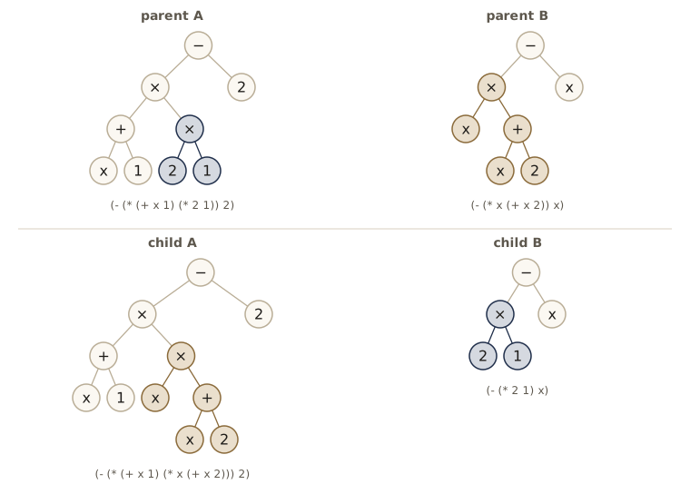
Now the evolution. The toy target is \(t(x) = 2x^2 - 3x + 1\) on 21 points in \([-2, 2]\), and the score to minimize is the mean squared error plus \(0.01\) per node, a parsimony penalty that discourages the trees from growing without bound (bloat). Parents are chosen by tournaments of three (the best of three random programs), the two best programs are copied unchanged, and each offspring comes from crossover (60%), mutation (25%), insertion (10%), or replication (5%).
xs = np.linspace(-2, 2, 21)
target = 2 * xs ** 2 - 3 * xs + 1

def gp_score(tree, alpha=0.01):
    return np.mean((evaluate(tree, xs) - target) ** 2) + alpha * tree_size(tree)

def genetic_program(L=200, generations=30, max_depth=6, seed=0, verbose=False):
    rng_gp = np.random.default_rng(seed)
    pop = [random_tree(3, rng_gp) for _ in range(L)]
    for g in range(generations):
        scores = np.array([gp_score(t) for t in pop])
        order = np.argsort(scores)
        if verbose and g % 5 == 0:
            print(f"generation {g:2d}: best score {scores[order[0]]:.4f}   {to_lisp(pop[order[0]])}")
        def tournament():
            idx = rng_gp.integers(L, size=3)
            return pop[idx[np.argmin(scores[idx])]]
        new = [pop[order[0]], pop[order[1]]]                   # replication of the two best
        while len(new) < L:
            r = rng_gp.random()
            if r < 0.60:
                kids = crossover(tournament(), tournament(), rng_gp)[:2]
            elif r < 0.85:
                kids = (mutate(tournament(), 0.15, rng_gp),)
            elif r < 0.95:
                kids = (insert(tournament(), rng_gp),)
            else:
                kids = (tournament(),)
            new += [k for k in kids if tree_depth(k) <= max_depth][: L - len(new)]   # depth wrapper
        pop = new
    scores = np.array([gp_score(t) for t in pop])
    return pop[int(np.argmin(scores))]

best_tree = genetic_program(seed=0, verbose=True)
mse = np.mean((evaluate(best_tree, xs) - target) ** 2)
print(f"final: {to_lisp(best_tree)}   size {tree_size(best_tree)}   MSE {mse:.2e}")
generation  0: best score 6.9367   (* (- (* 2 x) 1) x)
generation  5: best score 0.1500   (- (+ (+ 2 (* x (* x 2))) (- 2 (* 3 x))) 3)
generation 10: best score 0.1100   (- (- 1 x) (* x (- 2 (* x 2))))
generation 15: best score 0.1100   (- (- 1 x) (* x (- 2 (* x 2))))
generation 20: best score 0.1100   (- (- 1 x) (* x (- 2 (* x 2))))
generation 25: best score 0.1100   (- (- 1 x) (* x (- 2 (* x 2))))
final: (- (- 1 x) (* x (- 2 (* x 2))))   size 11   MSE 3.88e-31
The run finds an exact expression for the target: expanding it, \((1 - x) - x(2 - 2x) = 2x^2 - 3x + 1\). Different seeds find different programs that compute the same function, some of them with redundant pieces such as (* 2 1) that the parsimony penalty has not yet removed.
for seed in range(1, 6):
    t = genetic_program(seed=seed)
    print(f"seed {seed}: {to_lisp(t):40s} MSE {np.mean((evaluate(t, xs) - target) ** 2):.2e}")
seed 1: (* (- 1 x) (- (- 1 x) x))                MSE 3.42e-31
seed 2: (+ (- 1 (* 3 x)) (* x (* 2 x)))          MSE 9.68e-33
seed 3: (+ (* (* x (- x 1)) (* 2 1)) (- 1 x))    MSE 3.88e-31
seed 4: (- (* x x) (+ (* (- 3 x) x) (- 3 (* 2 2)))) MSE 2.13e-31
seed 5: (+ 1 (* x (- (* x 2) 3)))                MSE 2.29e-31
To use genetic programming as a classifier, evolve an expression \(g(\mathbf{x})\) of the features and assign category \(\omega_i\) when \(g(\mathbf{x}) > 0\) — a dichotomizer, one per category as with genetic algorithms — with accuracy as the fitness. Genetic programming has even less theory than genetic algorithms; experience in one domain transfers poorly to another, and it works best when the target can be expressed compactly with the chosen operators. Its appeal is that it searches over the form of the classifier, not only its parameters, and it gets more practical as computation gets cheaper.
Summary
| Method | What it searches | How randomness enters | What to watch |
|---|---|---|---|
| Greedy descent | configurations of \(\pm 1\) units | only in the start | stops in the first local minimum |
| Stochastic simulated annealing | configurations, one unit at a time | Metropolis acceptance of uphill moves at temperature \(T(k)\) | cooling rate; keep the best configuration seen |
| Deterministic (mean-field) annealing | averages \(m_i \in [-1, 1]\) | none (polling order only) | decisions happen below \(T_c = \lambda_{\max}(\mathbf{W})\); can lock into the wrong basin |
| Boltzmann learning | weights of a stochastic network | sampled correlations in clamped and free phases | cost of the two phases; hidden units for higher-order structure |
| Deterministic Boltzmann learning | weights | none; correlations \(\approx m_im_j\) | mean-field approximation of the correlations |
| Genetic algorithm | bit strings (chromosomes) | selection, crossover, mutation | selection pressure; representation; overfitting the score |
| Genetic programming | expression trees | subtree crossover, mutation, insertion | bloat; validity (wrapper); little theory |
Ideas to carry forward:
- The Boltzmann distribution \(P(\gamma) \propto e^{-E_\gamma/T}\) connects optimization and probability: at low temperature it concentrates on the minima, and a Markov chain that satisfies detailed balance samples it. Annealing is a way of sampling at a temperature too low to sample directly.
- Boltzmann learning is maximum likelihood for a network with an energy, and its gradient is always the same shape: a correlation with the data imposed minus a correlation with the network running freely. The same “clamped minus free” structure is the gradient of any exponential-family or energy-based model.
- Hidden units are what let pairwise interactions represent higher-order structure, as parity shows; without them a Boltzmann network matches only the means and pairwise correlations of the data.
- Stochastic search pays off when the space is huge and irregular, not when it is small: on our small examples brute force was cheaper. Whatever the search, if it optimizes a score measured on data, it can overfit that data.
Exercises
- Show that \(E(\mathbf{s}) = -\tfrac{1}{2}\mathbf{s}^{t}\mathbf{W}\mathbf{s}\) is unchanged when \(\mathbf{W}\) is replaced by \(\tfrac{1}{2}(\mathbf{W} + \mathbf{W}^{t})\), and that changing the diagonal of \(\mathbf{W}\) shifts every energy by the same constant. Then show that with a bias unit clamped at \(+1\), the energy of the other units is \(-\tfrac{1}{2}\mathbf{s}^{t}\mathbf{W}'\mathbf{s} - \mathbf{b}^{t}\mathbf{s}\) and identify \(\mathbf{W}'\) and \(\mathbf{b}\).
- Prove that greedy descent stops after finitely many flips, and bound the number of flips in terms of \(E_{\max} - E_{\min}\) and the smallest nonzero value of \(\lvert 2 s_i l_i \rvert\). Why does the code keep a unit’s state when its field is exactly zero?
- Show that the heat-bath update \(P(s_i = +1 \mid \text{rest}) = 1/(1 + e^{-2l_i/T})\) satisfies detailed balance with respect to the Boltzmann distribution. Then replace
metropolis_sweepby heat-bath sweeps inannealand compare the success rates on the 12-unit network for \(c = 0.9\) and \(c = 0.95\). - For a single unit in a fixed field \(l\), derive \(\mathbb{E}[s] = \tanh(l/T)\) and \(\operatorname{Var}(s) = 1 - \tanh^2(l/T)\). Use the variance to explain what the mean-field approximation throws away when it replaces \(\mathbb{E}[s_is_j]\) by \(m_im_j\).
- Show that for the parallel update \(\mathbf{m} \leftarrow \tanh(\mathbf{W}\mathbf{m}/T)\) the point \(\mathbf{m} = \mathbf{0}\) is stable for \(T > \max_k \lvert \lambda_k \rvert\). Then search over seeds for a 12-unit network (weights drawn as in the notes) on which mean-field annealing with \(c = 0.95\) finds the global minimum in fewer than 10% of runs while stochastic annealing still succeeds in more than 40%. Compare the energy of the sign pattern of the top eigenvector with the global minimum for that network.
- Derive the conditional learning rule, with inputs clamped in both phases, from the averaged conditional divergence \(\bar{D}_{\mathrm{KL}}\), writing out each log-sum-exp derivative.
- For a Boltzmann network with no hidden units, show that the Hessian of \(D_{\mathrm{KL}}\) with respect to the weights is \(1/T^2\) times the covariance matrix of the statistics \(s_is_j\) under \(P\), hence positive semidefinite. Conclude that the divergence is convex, and explain why this does not contradict the stalled divergence for parity.
- Give
train_visible_stochasticarguments for the annealing schedule and the number of collection sweeps. With annealed phases, measure the divergence floor (mean over the last 500 steps) for a longer anneal (say 14 temperatures with ratio 0.85) and for 10 collection sweeps; then run the persistent version with \(R = 50\), \(100\), and \(400\) chains. Plot the exact divergence against the total number of heat-bath sweeps used, and describe the trade-off between bias, noise, and cost. - Train the XOR classifier with four hidden units, with and without weight decay \(w_{ij} \leftarrow (1 - \epsilon)w_{ij}\) after every step. Report the final conditional divergence and the largest weight for \(\epsilon \in \{0, 10^{-3}, 10^{-2}\}\).
- For the Boltzmann chain of the notes, compute the posterior probability of every hidden path both from the HMM (path probability divided by \(P(\mathbf{V})\)) and from the Boltzmann distribution over legal configurations, and confirm they agree for two different temperatures. Why does the temperature drop out?
- Permute the columns of the feature data so that the informative features sit at positions 0, 5, 10, and 15. Rerun the comparison of 20 seeds with rank selection using one-point crossover and using uniform crossover (each bit from a random parent). Relate what you see to the defining length of the building-block schema.
- Change the genetic-programming target to \(x^3 - x\) and run ten seeds. Most runs stall at \(x^3\); compute the score of \(x^3\) and of the nearby expressions that would lead to \(x^3 - x\), and explain the failure as a deceptive landscape. Propose and test one change (to the operators, the terminal set, or the score) that helps.
- In your own words: simulated annealing, Boltzmann learning, and genetic algorithms all use randomness. For each, what exactly is random, what does the randomness buy, and what does it cost?
Going further
- R. O. Duda, P. E. Hart, and D. G. Stork, Pattern Classification, 2nd ed., chapter 7. Problems 2–8 (the energy, the Boltzmann factor, and the mean-field response), 11 (the conditional learning rule), 12–13 (Hopfield networks), 16–18 (hidden units, initial weights, and the learning rate), 19–22 (Boltzmann chains and zippers), and 24 (genetic-programming operators) pair with the sections above; Computer exercises 1–3 (search and annealing), 4–6 (Boltzmann classification and pattern completion), 8 (a genetic algorithm for tree classifiers), and 9 (genetic programming) extend the code.
- S. Kirkpatrick, C. D. Gelatt, and M. P. Vecchi, “Optimization by simulated annealing”, Science, 1983 — simulated annealing as a general optimization method. The acceptance rule comes from N. Metropolis, A. W. Rosenbluth, M. N. Rosenbluth, A. H. Teller, and E. Teller, “Equation of state calculations by fast computing machines”, Journal of Chemical Physics, 1953.
- D. H. Ackley, G. E. Hinton, and T. J. Sejnowski, “A learning algorithm for Boltzmann machines”, Cognitive Science, 1985 — the Boltzmann learning rule. J. J. Hopfield, “Neural networks and physical systems with emergent collective computational abilities”, PNAS, 1982 — the associative memory.
- D. J. C. MacKay, Information Theory, Inference, and Learning Algorithms (Cambridge, 2003; free online) — chapters on Monte Carlo methods, Hopfield networks, and Boltzmann machines, with a view complementary to this module’s.
- J. H. Holland, Adaptation in Natural and Artificial Systems (1975), and J. R. Koza, Genetic Programming (MIT Press, 1992) — the classic books on genetic algorithms (including the schema theorem) and on genetic programming.
- Intro to ML notes: module 11 for Markov chain Monte Carlo, Metropolis–Hastings, and Gibbs sampling; module 08 for Bayesian networks, Markov random fields, and the Ising model; module 13 for hidden Markov models.
These notes follow the chapters of R. O. Duda, P. E. Hart, and D. G. Stork, Pattern Classification, 2nd edition (Wiley, 2001), the course text. The explanations, code, figures, and exercises here are written for this course; the book remains the reference, with the full derivations, worked examples, and many more problems.