CSE 455/555 · Module 02 · Session 2
Bayesian Decision Theory
Risk and the Bayes decision rule, minimax and Neyman–Pearson, discriminant functions for Gaussian classes, error bounds and ROC curves, discrete and missing features, belief networks, and context.
Companion reading: Duda, Hart & Stork, Pattern Classification, chapter 2, “Bayesian Decision Theory”
By the end of this module you can
- Turn priors and class-conditional densities into posteriors with Bayes’ formula, and state and prove the rule that minimizes the probability of error.
- Set up a loss matrix, compute conditional risks, and derive the minimum-risk rule as a likelihood-ratio test, including a reject action.
- Find minimax and Neyman–Pearson decision rules numerically for a one-dimensional problem and explain what each one protects against.
- Write the discriminant functions for Gaussian classes in the three covariance cases, derive their decision boundaries, and implement a general quadratic discriminant.
- Compute a Bayes error by numerical integration and by Monte Carlo, split a non-optimal classifier’s error into Bayes and reducible parts, and evaluate the Chernoff and Bhattacharyya bounds.
- Relate the discriminability d′ to hit and false-alarm rates, draw an ROC curve, and pick an operating point from a loss matrix.
- Derive the linear discriminant for independent binary features, and classify with missing or noisy features by marginalizing.
- Compute probabilities in a small Bayesian belief network by enumeration, and explain how context between successive decisions changes the optimal rule.
Contents
- Priors, likelihoods, and posteriors
- Loss, risk, and the Bayes decision rule
- Minimum-error-rate classification
- Discriminant functions and decision surfaces
- The normal density
- Discriminant functions for the normal density
- Error probabilities and integrals
- Error bounds for normal densities
- Discrete features
- Missing and noisy features
- Bayesian belief networks
- Compound decision theory and context
- Summary
- Exercises
- Going further
In module 01 we took a pattern recognition system apart: a sensor, a segmenter, a feature extractor, a classifier, and a postprocessor. This module is about the classifier, in the idealized setting where we know everything there is to know about the probabilities involved. That sounds like a cheat, and in a sense it is: in practice the probabilities must be estimated from data, which is the business of module 03 and later modules. But the idealized setting tells us what the best possible classifier is, how often even that classifier must be wrong, and what “best” should mean when some mistakes cost more than others. Every classifier we build later is an attempt to approximate the rule derived here.
We follow chapter 2 of Duda, Hart & Stork, Pattern Classification (DHS from here on). Its angle is decision theory: actions, losses, decision regions, and the error rates they produce. The machine-learning notes cover some of the same ground from Bishop’s book, in particular the decision theory of Intro to ML, module 01 and the Gaussian identities of Intro to ML, module 02. We keep this module self-contained, but point there for longer derivations.
A word on notation. We use DHS’s conventions so that you can move between these notes and the book: categories \(\omega_1, \dots, \omega_c\), priors \(P(\omega_j)\), class-conditional densities \(p(\mathbf{x} \mid \omega_j)\), and the transpose written \(\mathbf{a}^{t}\). The ML notes write the same things as \(\mathcal{C}_k\), \(p(\mathcal{C}_k)\), and \(\mathbf{a}^{\mathrm{T}}\). Capital \(P\) is a probability, lowercase \(p\) a density.
Priors, likelihoods, and posteriors
Our running example is an inspection station on a production line. Each part that passes produces one measurement \(x\), a deviation score from a gauge. A part is either good (\(\omega_1\)) or defective (\(\omega_2\)), and which one it is we call the state of nature. Before we measure anything, we know from experience that about 80% of parts are good. These numbers, \(P(\omega_1) = 0.8\) and \(P(\omega_2) = 0.2\), are the prior probabilities (or priors): what we believe about the class before seeing the pattern. They must sum to one over the classes.
If we had to decide without measuring, the only sensible rule is to pick the class with the larger prior, here “good” every time. It is wrong exactly when the part is defective, so its probability of error is \(\min[P(\omega_1), P(\omega_2)] = 0.2\). No rule that ignores the measurement can do better.
The measurement helps because its distribution depends on the class. The class-conditional density \(p(x \mid \omega_j)\) is the density of \(x\) among parts of class \(\omega_j\). We will use
\[p(x \mid \omega_1) = \mathcal{N}(0, 1^2), \qquad p(x \mid \omega_2) = \mathcal{N}(3, 1.5^2),\]so defective parts score higher on average and vary more. Here \(\mathcal{N}(\mu, \sigma^2)\) is the normal density, which we study properly in a later section.
Once we measure \(x\), the joint density of class and measurement can be factored two ways, \(p(\omega_j, x) = P(\omega_j \mid x)\, p(x) = p(x \mid \omega_j)\, P(\omega_j)\). Solving for the first factor gives Bayes’ formula:
\[P(\omega_j \mid x) = \frac{p(x \mid \omega_j)\, P(\omega_j)}{p(x)}, \qquad p(x) = \sum_{k=1}^{c} p(x \mid \omega_k)\, P(\omega_k).\]The left side is the posterior probability of \(\omega_j\): our belief about the class after the measurement. Read as a function of \(j\) with \(x\) fixed, \(p(x \mid \omega_j)\) is called the likelihood of \(\omega_j\); a class under which the observed \(x\) is more probable has a larger likelihood. The denominator \(p(x)\) is the evidence. It does not depend on \(j\); its only job is to make the posteriors sum to one. In words: posterior = likelihood × prior / evidence.
The first code cell sets up the example. We work with log densities and normalize with log-sum-exp, a habit that will matter once we have many features.
import numpy as np
from scipy.special import logsumexp, ndtr, ndtri
from scipy.linalg import cho_factor, cho_solve, solve_triangular
from scipy import stats
from itertools import product

np.set_printoptions(precision=4, suppress=True)
rng = np.random.default_rng(455)

# running example: omega_1 = good part, omega_2 = defective part (index 0 and 1 in code)
mu = np.array([0.0, 3.0])       # class means
sd = np.array([1.0, 1.5])       # class standard deviations
prior = np.array([0.8, 0.2])    # P(omega_1), P(omega_2)

def log_normal_1d(x, m, s):
    """ln N(x; m, s^2), broadcasting over x, m, s."""
    return -0.5 * ((x - m) / s) ** 2 - np.log(s) - 0.5 * np.log(2 * np.pi)

def class_loglik(x):
    """ln p(x | omega_j) for every x (rows) and class j (columns)."""
    return log_normal_1d(np.asarray(x, dtype=float)[:, None], mu, sd)

def posteriors(x, prior=prior):
    """P(omega_j | x) by Bayes' formula, computed in log space."""
    a = class_loglik(x) + np.log(prior)
    return np.exp(a - logsumexp(a, axis=1, keepdims=True))

xs = np.array([-1.0, 1.0, 2.0, 3.0, 5.0])
post = posteriors(xs)
check = stats.norm.pdf(xs[:, None], mu, sd) * prior
check /= check.sum(axis=1, keepdims=True)
for x, p in zip(xs, post):
    print(f"x = {x:4.1f}:  P(w1|x) = {p[0]:.4f}   P(w2|x) = {p[1]:.4f}")
print(f"max difference from scipy.stats: {np.abs(post - check).max():.1e}")
x = -1.0:  P(w1|x) = 0.9922   P(w2|x) = 0.0078
x =  1.0:  P(w1|x) = 0.8985   P(w2|x) = 0.1015
x =  2.0:  P(w1|x) = 0.5035   P(w2|x) = 0.4965
x =  3.0:  P(w1|x) = 0.0625   P(w2|x) = 0.9375
x =  5.0:  P(w1|x) = 0.0001   P(w2|x) = 0.9999
max difference from scipy.stats: 1.1e-16
The posteriors sum to one at every \(x\) and move smoothly from “almost surely good” to “almost surely defective” as the score grows.
The rule that minimizes the probability of error
Having observed \(x\), suppose we decide \(\omega_1\). We are wrong with probability \(P(\omega_2 \mid x)\). If we decide \(\omega_2\), we are wrong with probability \(P(\omega_1 \mid x)\). To make the conditional probability of error \(P(\text{error} \mid x)\) as small as possible we should therefore
\[\text{decide } \omega_1 \text{ if } P(\omega_1 \mid x) > P(\omega_2 \mid x), \text{ otherwise decide } \omega_2,\]and then \(P(\text{error} \mid x) = \min[P(\omega_1 \mid x), P(\omega_2 \mid x)]\). This is the Bayes decision rule for minimum error. It also minimizes the average probability of error,
\[P(\text{error}) = \int_{-\infty}^{\infty} P(\text{error} \mid x)\, p(x)\, dx,\]because \(p(x) \ge 0\): a rule that makes the integrand as small as possible at every single \(x\) makes the integral as small as possible. That one-line argument, “minimize pointwise, and the average takes care of itself”, is the core of this whole chapter; we will reuse it with losses in place of errors.
Multiplying both posteriors by \(p(x)\) does not change which one is larger, so the rule can also be written without the evidence: decide \(\omega_1\) if \(p(x \mid \omega_1)P(\omega_1) > p(x \mid \omega_2)P(\omega_2)\). Two special cases show how the two factors share the work. Where the likelihoods are equal, the measurement is uninformative and the priors decide. Where the priors are equal, the likelihoods decide.
The minimum achievable error, the Bayes error, is the integral of the smaller of the two curves \(p(x \mid \omega_j)P(\omega_j)\). We compute it on a fine grid and compare it with the 0.2 of the rule that ignores \(x\).
x_grid = np.linspace(-12, 16, 56001)          # wide enough that the tails vanish
dx = x_grid[1] - x_grid[0]
joint = np.exp(class_loglik(x_grid)) * prior   # p(x | omega_j) P(omega_j)

bayes_error = np.minimum(joint[:, 0], joint[:, 1]).sum() * dx
print(f"error using priors only : {prior.min():.4f}")
print(f"Bayes error using x     : {bayes_error:.4f}")
print(f"integral of p(x)        : {joint.sum() * dx:.6f}")
error using priors only : 0.2000
Bayes error using x     : 0.0687
integral of p(x)        : 1.000000
Watch out. The priors belong to the situation where the classifier is used, not to the data set it was built from. If a training set was collected with equal numbers of good and defective parts but the line produces 20% defects, posteriors computed with the training proportions are wrong. The fix is cheap because the likelihoods do not change: recompute the posteriors with the deployment priors, which for two classes shifts the log odds by the log of the ratio of the new prior odds to the old ones.
Loss, risk, and the Bayes decision rule
Treating every error alike is often wrong. Shipping a defective part to a customer may cost far more than scrapping a good one. DHS generalize the setting in four directions at once: a feature vector \(\mathbf{x}\) in a \(d\)-dimensional feature space instead of a scalar, \(c\) classes instead of two, actions other than naming a class, and a cost attached to each action.
Actions, losses, and conditional risk
Let \(\alpha_1, \dots, \alpha_a\) be the possible actions. Usually \(\alpha_i\) means “decide \(\omega_i\)”, but an extra action such as “send the part to a human inspector” is allowed. The loss function \(\lambda(\alpha_i \mid \omega_j)\), written \(\lambda_{ij}\) for short, is the cost of taking action \(\alpha_i\) when the true class is \(\omega_j\). Having observed \(\mathbf{x}\), the true class is \(\omega_j\) with probability \(P(\omega_j \mid \mathbf{x})\), so the expected loss of action \(\alpha_i\) is
\[R(\alpha_i \mid \mathbf{x}) = \sum_{j=1}^{c} \lambda(\alpha_i \mid \omega_j)\, P(\omega_j \mid \mathbf{x}).\]In decision theory an expected loss is a risk, and \(R(\alpha_i \mid \mathbf{x})\) is the conditional risk of action \(\alpha_i\).
A decision rule \(\alpha(\mathbf{x})\) assigns an action to every point of feature space. Its overall risk is the conditional risk of the action it chooses, averaged over all \(\mathbf{x}\):
\[R = \int R(\alpha(\mathbf{x}) \mid \mathbf{x})\, p(\mathbf{x})\, d\mathbf{x}.\]The pointwise argument from the previous section applies unchanged. If at every \(\mathbf{x}\) we take the action with the smallest conditional risk, the integrand is as small as it can be everywhere, and so is \(R\).
Result. The Bayes decision rule: at each \(\mathbf{x}\), compute \(R(\alpha_i \mid \mathbf{x})\) for \(i = 1, \dots, a\) and take the action with the smallest value (ties may be broken any way). No other rule has smaller overall risk. The risk it achieves, \(R^{*}\), is the Bayes risk.
In code, the conditional risks for all actions are one matrix product: the loss matrix, with rows for actions and columns for classes, times the vector of posteriors.
def conditional_risk(x, Lam, prior=prior):
    """R(alpha_i | x) for every x (rows) and action i (columns).
    Lam[i, j] = lambda(alpha_i | omega_j)."""
    return posteriors(x, prior) @ Lam.T

def overall_risk(actions, Lam, prior=prior):
    """R = sum_x R(alpha(x) | x) p(x) dx on x_grid; the rule is an action index per grid point."""
    p_joint = np.exp(class_loglik(x_grid)) * prior        # p(x | omega_j) P(omega_j)
    # sum over x and j of lambda(alpha(x) | omega_j) p(x, omega_j) dx
    return (Lam[actions] * p_joint).sum() * dx

Lam_01 = np.array([[0.0, 1.0],       # decide good:      0 if good, 1 if defective
                   [1.0, 0.0]])      # decide defective: 1 if good, 0 if defective
Lam_ship = np.array([[0.0, 8.0],     # shipping a defective part costs 8
                     [1.0, 0.0]])    # scrapping a good part costs 1

for name, Lam in [("zero-one loss", Lam_01), ("shipping loss", Lam_ship)]:
    act = conditional_risk(x_grid, Lam).argmin(axis=1)     # Bayes rule on the grid
    boundary = x_grid[np.flatnonzero(np.diff(act))]       # where the chosen action switches
    print(f"{name}: switches at x = {np.round(boundary, 3)},  "
          f"Bayes risk = {overall_risk(act, Lam):.4f}")
zero-one loss: switches at x = [-6.806  2.005],  Bayes risk = 0.0687
shipping loss: switches at x = [-5.853  1.053],  Bayes risk = 0.2724
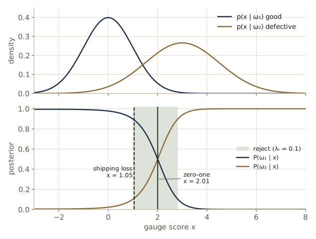
With zero-one loss the rule decides “defective” above about 2.0; with the shipping loss the threshold drops to about 1.05, because each defect we let through now costs eight times as much as a scrapped good part. The rule also switches at a second point far out on the left. We will see why in a moment.
Does the Bayes rule really beat everything else? A quick check: evaluate the overall shipping risk of many single-threshold rules, “decide defective when \(x > \tau\)”, and look for the best one.
taus = np.linspace(-1, 4, 501)
risks = [overall_risk((x_grid > tau).astype(int), Lam_ship) for tau in taus]
best = int(np.argmin(risks))
print(f"best single threshold: tau = {taus[best]:.3f}, risk = {risks[best]:.4f}")
risk_2 = overall_risk((x_grid > 2.0).astype(int), Lam_ship)
print(f"risk at the zero-one threshold tau = 2.0: {risk_2:.4f}")
best single threshold: tau = 1.050, risk = 0.2724
risk at the zero-one threshold tau = 2.0: 0.4223
The search lands on the Bayes threshold and cannot go below the Bayes risk. Using the zero-one threshold when the real costs are asymmetric is noticeably worse.
Two-category classification and the likelihood ratio
With two classes and the two actions “decide \(\omega_1\)” and “decide \(\omega_2\)”, the conditional risks are
\[\begin{aligned} R(\alpha_1 \mid \mathbf{x}) &= \lambda_{11} P(\omega_1 \mid \mathbf{x}) + \lambda_{12} P(\omega_2 \mid \mathbf{x}), \\ R(\alpha_2 \mid \mathbf{x}) &= \lambda_{21} P(\omega_1 \mid \mathbf{x}) + \lambda_{22} P(\omega_2 \mid \mathbf{x}). \end{aligned}\]We decide \(\omega_1\) when \(R(\alpha_1 \mid \mathbf{x}) < R(\alpha_2 \mid \mathbf{x})\). Collecting terms, that is when
\[(\lambda_{21} - \lambda_{11})\, P(\omega_1 \mid \mathbf{x}) > (\lambda_{12} - \lambda_{22})\, P(\omega_2 \mid \mathbf{x}).\]Normally a mistake costs more than a correct decision, so both factors in parentheses are positive. Replacing each posterior by likelihood × prior (the evidence cancels) and dividing gives the likelihood-ratio form: decide \(\omega_1\) if
\[\frac{p(\mathbf{x} \mid \omega_1)}{p(\mathbf{x} \mid \omega_2)} > \frac{\lambda_{12} - \lambda_{22}}{\lambda_{21} - \lambda_{11}} \cdot \frac{P(\omega_2)}{P(\omega_1)} .\]The left side depends only on the observation. The right side is a single number that collects everything else: the costs and the priors. So the Bayes rule for two classes is always a likelihood-ratio test: compute the ratio, compare it with a fixed threshold. Changing the costs or the priors never changes the ratio, only the threshold.
This explains the second switching point in the output above. For our two Gaussians, the log likelihood ratio \(\ln p(x \mid \omega_2) - \ln p(x \mid \omega_1)\) is a quadratic in \(x\). Because the defective class has the larger variance, the quadratic opens upward: the ratio favors “defective” at both ends of the line, and the region where we decide \(\omega_2\) is the union of two half-lines. The left piece starts near \(x = -6.8\), where almost no parts ever land, but it is part of the optimal rule. Decision regions do not have to be connected.
Writing the log likelihood ratio as \(q(x) = a x^2 + b x + c_0\), with
\[a = \frac{1}{2\sigma_1^2} - \frac{1}{2\sigma_2^2}, \qquad b = \frac{\mu_2}{\sigma_2^2} - \frac{\mu_1}{\sigma_1^2}, \qquad c_0 = \frac{\mu_1^2}{2\sigma_1^2} - \frac{\mu_2^2}{2\sigma_2^2} + \ln\frac{\sigma_1}{\sigma_2},\]the test “decide \(\omega_2\) when \(q(x) > t\)” has the region \(x < r_{-}\) or \(x > r_{+}\), where \(r_{\pm}\) are the roots of \(q(x) = t\). The probabilities of landing there under each class are differences of normal distribution functions \(\Phi\). The two that matter most get names borrowed from detection problems: the false-alarm rate \(P(\text{decide } \omega_2 \mid \omega_1)\) and the hit rate \(P(\text{decide } \omega_2 \mid \omega_2)\). The next cell computes them exactly; we will use this function for minimax, Neyman–Pearson, and ROC curves.
a_q = 1 / (2 * sd[0]**2) - 1 / (2 * sd[1]**2)
b_q = mu[1] / sd[1]**2 - mu[0] / sd[0]**2
c_q = mu[0]**2 / (2 * sd[0]**2) - mu[1]**2 / (2 * sd[1]**2) + np.log(sd[0] / sd[1])

def lr_test(t):
    """Decide omega_2 when ln p(x|w2) - ln p(x|w1) > t.
    Returns (r_minus, r_plus, false_alarm, hit)."""
    disc = b_q**2 - 4 * a_q * (c_q - t)
    if disc <= 0:            # the quadratic exceeds t everywhere: always decide omega_2
        return -np.inf, np.inf, 1.0, 1.0
    r_m, r_p = (-b_q - np.sqrt(disc)) / (2 * a_q), (-b_q + np.sqrt(disc)) / (2 * a_q)
    # P(x < r_m or x > r_p | omega_j) for both classes at once
    rate = ndtr((r_m - mu) / sd) + 1 - ndtr((r_p - mu) / sd)
    return r_m, r_p, rate[0], rate[1]

def bayes_risk_of_test(t, Lam, prior=prior):
    """Overall risk of the test: sum_ij lambda_ij P(omega_j) P(decide i | omega_j)."""
    _, _, fa, hit = lr_test(t)
    P_dec = np.array([[1 - fa, 1 - hit],      # P(decide omega_1 | omega_j)
                      [fa, hit]])             # P(decide omega_2 | omega_j)
    return (Lam * P_dec * prior).sum()

# the Bayes threshold on the log ratio for a loss matrix and priors
def bayes_log_threshold(Lam, prior=prior):
    return np.log((Lam[1, 0] - Lam[0, 0]) * prior[0] / ((Lam[0, 1] - Lam[1, 1]) * prior[1]))

for name, Lam in [("zero-one", Lam_01), ("shipping", Lam_ship)]:
    t = bayes_log_threshold(Lam)
    r_m, r_p, fa, hit = lr_test(t)
    print(f"{name:8s}: t = {t:7.4f}  region x < {r_m:.3f} or x > {r_p:.3f}  "
          f"FA = {fa:.4f}  hit = {hit:.4f}  risk = {bayes_risk_of_test(t, Lam):.4f}")
zero-one: t =  1.3863  region x < -6.806 or x > 2.006  FA = 0.0224  hit = 0.7463  risk = 0.0687
shipping: t = -0.6931  region x < -5.853 or x > 1.053  FA = 0.1461  hit = 0.9028  risk = 0.2724
The exact risks agree with the grid integrals of the previous cell to four decimals, and the boundaries agree with the switching points.
Minimum-error-rate classification
In classification the actions are usually just “decide \(\omega_i\)”, and often all errors are equally bad. The loss that expresses this is the zero–one loss,
\[\lambda(\alpha_i \mid \omega_j) = \begin{cases} 0 & i = j, \\ 1 & i \ne j, \end{cases} \qquad i, j = 1, \dots, c.\]Its conditional risk is
\[R(\alpha_i \mid \mathbf{x}) = \sum_{j \ne i} P(\omega_j \mid \mathbf{x}) = 1 - P(\omega_i \mid \mathbf{x}),\]which is exactly the probability that deciding \(\omega_i\) is wrong. So the overall risk is the error rate, and minimizing risk means choosing the class with the largest posterior:
\[\text{decide } \omega_i \text{ if } P(\omega_i \mid \mathbf{x}) > P(\omega_j \mid \mathbf{x}) \text{ for all } j \ne i.\]This is the maximum a posteriori (MAP) rule, and it is the rule we met in the first section, now justified for any number of classes. The set of points where it decides \(\omega_i\) is the decision region \(\mathcal{R}_i\).
A reject option
Sometimes it is better not to decide. Suppose that, besides the \(c\) class decisions with zero–one loss, we may reject the pattern (hand it to a human, ask for another measurement) at a fixed cost \(\lambda_r\) between 0 and 1, whatever the class. The conditional risk of rejecting is \(\lambda_r\), and the smallest risk among the class decisions is \(1 - \max_i P(\omega_i \mid \mathbf{x})\). So the Bayes rule becomes:
\[\text{decide the MAP class if } \max_i P(\omega_i \mid \mathbf{x}) \ge 1 - \lambda_r, \text{ otherwise reject.}\]A cheap reject (\(\lambda_r\) near 0) rejects almost everything; once \(\lambda_r \ge (c-1)/c\) it never rejects, since the largest posterior is always at least \(1/c\). In between we trade rejections against errors. The next cell shows this trade for the inspection problem: as rejecting gets more expensive, we reject less and accept more errors.
def reject_rule(x, lam_r, prior=prior):
    """Returns (action, P_max): action 0..c-1 for a class, c for reject."""
    post = posteriors(x, prior)
    p_max = post.max(axis=1)
    return np.where(p_max >= 1 - lam_r, post.argmax(axis=1), post.shape[1]), p_max

p_joint = np.exp(class_loglik(x_grid)) * prior
print(" lam_r   reject rate   error rate   overall risk")
for lam_r in [0.05, 0.10, 0.20, 0.30, 0.50]:
    act, _ = reject_rule(x_grid, lam_r)
    rej = (act == 2)
    # errors: decided omega_2 on a good part, or omega_1 on a defective one
    err = ((p_joint[:, 0] * (act == 1)).sum() + (p_joint[:, 1] * (act == 0)).sum()) * dx
    rej_rate = (p_joint.sum(axis=1) * rej).sum() * dx
    print(f"  {lam_r:.2f}    {rej_rate:9.4f}    {err:9.4f}     {err + lam_r * rej_rate:9.4f}")
 lam_r   reject rate   error rate   overall risk
  0.05       0.3208       0.0113        0.0274
  0.10       0.1995       0.0199        0.0399
  0.20       0.1079       0.0330        0.0545
  0.30       0.0616       0.0444        0.0628
  0.50       0.0000       0.0687        0.0687
With \(\lambda_r = 0.1\) we reject about a fifth of the parts and cut the error rate from 0.069 to 0.020. The last row, \(\lambda_r = 0.5 = (c-1)/c\), never rejects and reproduces the plain Bayes error. Notice that the overall risk increases with \(\lambda_r\): the more a rejection costs, the less the option is worth.
The figure shows the whole story for the inspection problem: the two class-conditional densities, the posteriors, the zero–one boundary, the boundary under the shipping loss, and the band of scores rejected when \(\lambda_r = 0.1\).
The minimax criterion
The Bayes rule is optimal for the priors it was designed with. Suppose the defect rate is not stable: a new supplier, a worn tool, or a second factory using the same classifier. What happens to a fixed rule when the prior moves?
Fix the decision regions \(\mathcal{R}_1\) and \(\mathcal{R}_2\) and name the two conditional error rates
\[\varepsilon_1 = \int_{\mathcal{R}_2} p(\mathbf{x} \mid \omega_1)\, d\mathbf{x}, \qquad \varepsilon_2 = \int_{\mathcal{R}_1} p(\mathbf{x} \mid \omega_2)\, d\mathbf{x},\]the probability that a pattern of class \(\omega_1\) lands in the region for \(\omega_2\), and vice versa. The overall risk is the loss of each outcome times its probability. Writing \(P(\omega_2) = 1 - P(\omega_1)\),
\[R = \big[\lambda_{22} + (\lambda_{12} - \lambda_{22})\,\varepsilon_2\big] + P(\omega_1)\Big[\lambda_{11} + (\lambda_{21} - \lambda_{11})\,\varepsilon_1 - \lambda_{22} - (\lambda_{12} - \lambda_{22})\,\varepsilon_2\Big].\]Once the regions are fixed, \(\varepsilon_1\) and \(\varepsilon_2\) are fixed, so the risk of a fixed rule is a straight line in the prior \(P(\omega_1)\). Its worst case is at one of the ends, \(P(\omega_1) = 0\) or \(1\), unless the slope is zero. The minimax rule is the rule whose worst-case risk over all priors is smallest.
Here is why it is found by making the slope vanish. Let \(R^{*}(P)\) be the Bayes risk when \(P(\omega_1) = P\). Because \(R^{*}\) is at each prior the minimum over all rules of their straight lines, it is a concave curve, and the line of the Bayes rule designed for prior \(P_0\) lies above the curve and touches it at \(P_0\). Every rule’s line lies on or above \(R^{*}\), so every rule has worst-case risk at least \(\max_P R^{*}(P)\). The Bayes rule for the prior that maximizes \(R^{*}\), the least favorable prior, has a horizontal tangent line there, so its risk equals \(\max_P R^{*}\) for every prior and attains that lower bound. The minimax risk is therefore
\[R_{mm} = \lambda_{22} + (\lambda_{12} - \lambda_{22})\,\varepsilon_2 = \lambda_{11} + (\lambda_{21} - \lambda_{11})\,\varepsilon_1 ,\]and for zero–one loss the condition is simply \(\varepsilon_1 = \varepsilon_2\): the two kinds of error are equally likely. (For densities with atoms or flat stretches a horizontal tangent may not exist, and the minimax rule has to be randomized; with our continuous densities this does not arise.)
We compute the minimax rule for the inspection problem with zero–one loss in two independent ways: by maximizing the Bayes error over a grid of priors, and by solving \(\varepsilon_1 = \varepsilon_2\) for the likelihood-ratio threshold with bisection.
def bisect(f, lo, hi, tol=1e-12):
    """Root of f on [lo, hi] by bisection; f(lo) and f(hi) must have opposite signs."""
    f_lo = f(lo)
    while hi - lo > tol:
        mid = 0.5 * (lo + hi)
        if (f(mid) > 0) == (f_lo > 0):
            lo, f_lo = mid, f(mid)
        else:
            hi = mid
    return 0.5 * (lo + hi)

def error_of_test(t, P1):
    """Error rate of the test with log threshold t when P(omega_1) = P1."""
    _, _, fa, hit = lr_test(t)
    return P1 * fa + (1 - P1) * (1 - hit)

# (1) the Bayes error curve R*(P1); its maximum is the minimax risk
P1s = np.linspace(0.001, 0.999, 999)
R_star = np.array([error_of_test(np.log(P / (1 - P)), P) for P in P1s])
i = R_star.argmax()
print(f"max Bayes error over priors : {R_star[i]:.4f} at P(w1) = {P1s[i]:.3f}")

# (2) the threshold where epsilon_1 = epsilon_2 (false alarm = miss)
t_mm = bisect(lambda t: lr_test(t)[2] - (1 - lr_test(t)[3]), -5, 5)
r_m, r_p, fa, hit = lr_test(t_mm)
print(f"minimax test: t = {t_mm:.4f}, decide w2 for x > {r_p:.4f};  "
      f"eps1 = {fa:.4f}, eps2 = {1 - hit:.4f}")
print(f"least favorable prior from t: P(w1) = {np.exp(t_mm) / (1 + np.exp(t_mm)):.4f}")

# the rule designed for P(w1) = 0.8, evaluated at the extreme priors
t08 = np.log(0.8 / 0.2)
print(f"rule designed for P(w1)=0.8: error {error_of_test(t08, 0.0):.4f} if all parts "
      f"are defective, {error_of_test(t08, 1.0):.4f} if all are good")
max Bayes error over priors : 0.1151 at P(w1) = 0.400
minimax test: t = -0.4055, decide w2 for x > 1.2000;  eps1 = 0.1151, eps2 = 0.1151
least favorable prior from t: P(w1) = 0.4000
rule designed for P(w1)=0.8: error 0.2537 if all parts are defective, 0.0224 if all are good
Both methods agree. The minimax rule puts its threshold lower than the rule designed for an 80% good rate, and its error is the same whatever the defect rate turns out to be. The price is that for the prior we actually expect, \(P(\omega_1) = 0.8\), it is worse than the Bayes rule: its error there is its constant \(R_{mm} = 0.115\), compared with the Bayes error of 0.069. The least favorable prior, \(P(\omega_1) = 0.4\), is the one that makes the classes hardest to tell apart. The rule designed for \(P(\omega_1) = 0.8\) is excellent near that prior but misses about a quarter of the defects, which is its error when every part is defective.
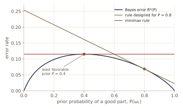
Minimax thinking comes from game theory, where an opponent picks the worst case on purpose. In pattern recognition it is a defensive choice when priors are unknown and may shift, and it is used less often than the Bayes rule.
The Neyman–Pearson criterion
A different way to handle one especially important kind of error is to put a hard limit on it. Suppose a contract says that at most 5% of good parts may be scrapped. We want the rule that catches as many defects as possible subject to \(\varepsilon_1 \le \alpha = 0.05\). This is the Neyman–Pearson criterion: maximize the hit rate subject to a bound on the false-alarm rate. Notice that it needs no priors and no losses.
The solution is again a likelihood-ratio test. Maximizing \(\int_{\mathcal{R}_2} p(\mathbf{x} \mid \omega_2)\,d\mathbf{x}\) subject to \(\int_{\mathcal{R}_2} p(\mathbf{x} \mid \omega_1)\,d\mathbf{x} = \alpha\) with a Lagrange multiplier \(\theta \ge 0\) means maximizing
\[\int_{\mathcal{R}_2} \big[p(\mathbf{x} \mid \omega_2) - \theta\, p(\mathbf{x} \mid \omega_1)\big]\, d\mathbf{x} + \theta\alpha\]over regions \(\mathcal{R}_2\). The pointwise argument once more: include \(\mathbf{x}\) in \(\mathcal{R}_2\) exactly when the bracket is positive, that is, when \(p(\mathbf{x} \mid \omega_2)/p(\mathbf{x} \mid \omega_1) > \theta\), and pick \(\theta\) so that the false-alarm rate equals \(\alpha\). This is the Neyman–Pearson lemma. Comparing with the likelihood-ratio form of the Bayes rule, a Neyman–Pearson rule is the Bayes rule for some combination of costs and priors: the constraint fixes the threshold instead of the losses doing it.
In code, the false-alarm rate of lr_test decreases as the threshold grows, so bisection finds the threshold that meets the constraint.
alpha = 0.05
t_np = bisect(lambda t: lr_test(t)[2] - alpha, -5, 10)
r_m, r_p, fa, hit = lr_test(t_np)
print(f"Neyman-Pearson test: t = {t_np:.4f} (theta = {np.exp(t_np):.4f}), "
      f"decide w2 for x > {r_p:.4f}")
print(f"false-alarm rate = {fa:.4f}, hit rate = {hit:.4f}")

# the same rule is the Bayes rule for the cost ratio
# (lambda_12 - lambda_22) / (lambda_21 - lambda_11) below
implied = prior[0] / (prior[1] * np.exp(t_np))
print(f"implied cost of a shipped defect, in scrapped good parts: {implied:.3f}")

# the multiplier theta is the slope d(hit)/d(false alarm) of the curve traced by the threshold
h = 1e-4
_, _, fa_a, hit_a = lr_test(t_np - h)
_, _, fa_b, hit_b = lr_test(t_np + h)
print(f"finite-difference slope d(hit)/d(FA) = {(hit_b - hit_a) / (fa_b - fa_a):.4f}")
Neyman-Pearson test: t = 0.5392 (theta = 1.7147), decide w2 for x > 1.6449
false-alarm rate = 0.0500, hit rate = 0.8169
implied cost of a shipped defect, in scrapped good parts: 2.333
finite-difference slope d(hit)/d(FA) = 1.7147
Capping false alarms at 5% catches about 82% of the defects. With our priors that is the same rule as the Bayes rule for a shipped defect costing about 2.3 times a scrapped good part. (The threshold 1.645 is the 95th percentile of the good-part density: the far-left piece of the region contributes almost nothing to the false alarms.) The last line anticipates the receiver operating characteristic of a later section: as the threshold varies, the pair (false alarm, hit) traces a curve, and at every point its slope equals the likelihood-ratio threshold \(\theta\) that produces that point.
Discriminant functions and decision surfaces
The multicategory case
A convenient way to describe any classifier, Bayes or not, is by a set of discriminant functions \(g_i(\mathbf{x})\), \(i = 1, \dots, c\): the classifier assigns \(\mathbf{x}\) to \(\omega_i\) if
\[g_i(\mathbf{x}) > g_j(\mathbf{x}) \quad \text{for all } j \ne i.\]Picture a machine with \(d\) inputs feeding \(c\) boxes, each computing one \(g_i\), followed by a selector that reports which box produced the largest value. The Bayes classifier fits this form with \(g_i(\mathbf{x}) = -R(\alpha_i \mid \mathbf{x})\) (largest discriminant = smallest risk), and for minimum error with \(g_i(\mathbf{x}) = P(\omega_i \mid \mathbf{x})\).
The discriminant functions are far from unique. Replacing every \(g_i\) by \(f(g_i)\), with the same monotonically increasing \(f\) for all classes, changes no decision. For minimum error this gives three equivalent choices,
\[g_i(\mathbf{x}) = P(\omega_i \mid \mathbf{x}), \qquad g_i(\mathbf{x}) = p(\mathbf{x} \mid \omega_i)\,P(\omega_i), \qquad g_i(\mathbf{x}) = \ln p(\mathbf{x} \mid \omega_i) + \ln P(\omega_i),\]and the last is the one we compute with. Any classifier divides feature space into decision regions \(\mathcal{R}_1, \dots, \mathcal{R}_c\), where \(\mathcal{R}_i\) is the set of points with \(g_i\) largest. They are separated by decision boundaries, the surfaces where the two largest discriminants tie.
The logarithm is more than a convenience. In the next cell, two classes have 1000 independent unit-variance features each. Every factor of the class-conditional density is below \(0.4\), so the product underflows to zero in floating point for both classes, and the first two forms cannot tell the classes apart. The log form has no trouble.
d_big = 1000
m_a, m_b = np.zeros(d_big), np.full(d_big, 0.1)        # two means, 1000 features
x_big = rng.normal(m_b, 1.0)                          # a pattern from the second class

# p(x | omega) as a product of 1000 densities
p_a = np.prod(np.exp(log_normal_1d(x_big, m_a, 1.0)))
p_b = np.prod(np.exp(log_normal_1d(x_big, m_b, 1.0)))
g_a = log_normal_1d(x_big, m_a, 1.0).sum() + np.log(0.5)
g_b = log_normal_1d(x_big, m_b, 1.0).sum() + np.log(0.5)
print(f"products of densities: {p_a:.3e} and {p_b:.3e}")
decision = "b" if g_b > g_a else "a"
print(f"log discriminants    : {g_a:.2f} and {g_b:.2f}  -> decide class {decision}")
print(f"posterior of class b : {np.exp(g_b - logsumexp([g_a, g_b])):.4f}")
products of densities: 0.000e+00 and 0.000e+00
log discriminants    : -1387.72 and -1385.51  -> decide class b
posterior of class b : 0.9014
The two-category case
With two classes one discriminant is enough. Define \(g(\mathbf{x}) = g_1(\mathbf{x}) - g_2(\mathbf{x})\) and decide \(\omega_1\) when \(g(\mathbf{x}) > 0\). A classifier for two classes is called a dichotomizer; it computes a single function and looks at its sign. Two forms of the minimum-error dichotomizer are especially handy:
\[g(\mathbf{x}) = P(\omega_1 \mid \mathbf{x}) - P(\omega_2 \mid \mathbf{x}), \qquad g(\mathbf{x}) = \ln \frac{p(\mathbf{x} \mid \omega_1)}{p(\mathbf{x} \mid \omega_2)} + \ln \frac{P(\omega_1)}{P(\omega_2)}.\]The second is the log likelihood ratio plus a constant, the likelihood-ratio test again. For the inspection problem it is \(g(x) = -q(x) + \ln 4\), a downward-opening quadratic in \(x\), positive on the interval between the two boundary points we found. Linear discriminants, which make \(g\) linear in \(\mathbf{x}\), are the subject of module 05; the next sections show when the Bayes dichotomizer itself is linear.
The normal density
The shape of a Bayes classifier comes from the class-conditional densities and the priors. The density studied most is the normal, or Gaussian, for two reasons: it is analytically convenient, and it is a reasonable model of a class whose patterns are a single prototype corrupted by many small, independent disturbances. (The ML notes collect the Gaussian identities with full proofs in Intro to ML, module 02.)
Recall that the expected value of a function \(f(x)\) under a density \(p(x)\) is \(\mathcal{E}[f(x)] = \int f(x)\,p(x)\,dx\), or a sum \(\sum_{x} f(x)P(x)\) over the possible values when \(x\) is discrete.
Univariate density
The univariate normal density with mean \(\mu\) and variance \(\sigma^2\) is
\[p(x) = \frac{1}{\sqrt{2\pi}\,\sigma} \exp\left[-\frac{1}{2}\left(\frac{x - \mu}{\sigma}\right)^2\right],\]written \(p(x) \sim N(\mu, \sigma^2)\), with \(\mu = \mathcal{E}[x]\) and \(\sigma^2 = \mathcal{E}[(x - \mu)^2]\). Its peak height is \(1/(\sqrt{2\pi}\sigma)\), and about 95% of its mass lies within \(2\sigma\) of the mean.
The entropy of a density,
\[H(p) = -\int p(x) \ln p(x)\, dx,\]measures how uncertain a draw from it is, in nats (in bits if the logarithm is base 2). For the normal density \(H = \tfrac12 \ln(2\pi e \sigma^2)\). Among all densities with a given variance, the normal has the largest entropy (DHS Problem 20 asks for the proof, a short calculus-of-variations argument): it assumes the least beyond the first two moments. Together with the central limit theorem, which says that a sum of many small independent effects is approximately normal, this is the usual justification for Gaussian class models. The next cell checks the moments and the entropy by numerical integration, and compares the entropy with two other densities of variance one.
x1 = np.linspace(-12, 12, 240001); h1 = x1[1] - x1[0]
p1 = np.exp(log_normal_1d(x1, 0.0, 1.0))
print(f"mean {np.sum(x1 * p1) * h1:.4f}   variance {np.sum(x1**2 * p1) * h1:.4f}   "
      f"mass within 2 sigma {np.sum(p1[np.abs(x1) < 2]) * h1:.4f}")
H_num = -np.sum(p1 * np.log(p1)) * h1
H_formula = 0.5 * np.log(2 * np.pi * np.e)
print(f"entropy of N(0,1): numerical {H_num:.4f}, formula {H_formula:.4f}")
# other densities with variance 1: uniform of width sqrt(12), Laplace with scale 1/sqrt(2)
print(f"entropy of uniform {np.log(np.sqrt(12)):.4f},  "
      f"Laplace {1 + np.log(2 / np.sqrt(2)):.4f}")
mean 0.0000   variance 1.0000   mass within 2 sigma 0.9545
entropy of N(0,1): numerical 1.4189, formula 1.4189
entropy of uniform 1.2425,  Laplace 1.3466
Multivariate density
In \(d\) dimensions the normal density with mean vector \(\boldsymbol{\mu}\) and covariance matrix \(\boldsymbol{\Sigma}\) is
\[p(\mathbf{x}) = \frac{1}{(2\pi)^{d/2} \lvert \boldsymbol{\Sigma} \rvert^{1/2}} \exp\left[-\frac{1}{2}(\mathbf{x} - \boldsymbol{\mu})^{t} \boldsymbol{\Sigma}^{-1} (\mathbf{x} - \boldsymbol{\mu})\right],\]written \(p(\mathbf{x}) \sim N(\boldsymbol{\mu}, \boldsymbol{\Sigma})\), where \(\lvert \boldsymbol{\Sigma} \rvert\) is the determinant. The parameters are the expectations
\[\boldsymbol{\mu} = \mathcal{E}[\mathbf{x}], \qquad \boldsymbol{\Sigma} = \mathcal{E}\big[(\mathbf{x} - \boldsymbol{\mu})(\mathbf{x} - \boldsymbol{\mu})^{t}\big],\]taken component by component, so \(\sigma_{ij} = \mathcal{E}[(x_i - \mu_i)(x_j - \mu_j)]\). The covariance matrix is symmetric and positive semidefinite; we always assume it is positive definite, so that \(\lvert \boldsymbol{\Sigma} \rvert > 0\). (If it is only semidefinite, the data lie in a lower-dimensional subspace, for example because one feature is a multiple of another, and the density does not exist in \(d\) dimensions.) Its diagonal entries \(\sigma_{ii} = \sigma_i^2\) are the variances of the features, and the off-diagonal entries are their covariances. If \(x_i\) and \(x_j\) are statistically independent then \(\sigma_{ij} = 0\); for a normal density the converse also holds, so a diagonal \(\boldsymbol{\Sigma}\) makes \(p(\mathbf{x})\) the product of \(d\) univariate normals. The density has \(d + d(d+1)/2\) free parameters: the mean and the upper triangle of \(\boldsymbol{\Sigma}\).
We evaluate the log density through the Cholesky factorization \(\boldsymbol{\Sigma} = \mathbf{L}\mathbf{L}^{t}\), with \(\mathbf{L}\) lower triangular. Then \((\mathbf{x} - \boldsymbol{\mu})^{t}\boldsymbol{\Sigma}^{-1}(\mathbf{x} - \boldsymbol{\mu}) = \lVert \mathbf{z} \rVert^2\) with \(\mathbf{z} = \mathbf{L}^{-1}(\mathbf{x} - \boldsymbol{\mu})\), one triangular solve, and \(\ln \lvert \boldsymbol{\Sigma} \rvert = 2\sum_i \ln L_{ii}\). No inverse is ever formed. The same factor gives a sampler: if \(\mathbf{u} \sim N(\mathbf{0}, \mathbf{I})\) then \(\boldsymbol{\mu} + \mathbf{L}\mathbf{u} \sim N(\boldsymbol{\mu}, \boldsymbol{\Sigma})\).
def mahalanobis2(X, m, S):
    """Squared Mahalanobis distance (x - m)^t S^{-1} (x - m) for each row of X."""
    L = np.linalg.cholesky(S)
    Z = solve_triangular(L, (np.atleast_2d(X) - m).T, lower=True)   # L^{-1}(x - m)
    return (Z**2).sum(axis=0)

def log_gauss(X, m, S):
    """ln N(x; m, S) for each row of X."""
    L = np.linalg.cholesky(S)
    logdet = 2 * np.log(np.diag(L)).sum()
    return -0.5 * (mahalanobis2(X, m, S) + logdet + len(m) * np.log(2 * np.pi))

def sample_gauss(n, m, S, gen):
    return m + gen.standard_normal((n, len(m))) @ np.linalg.cholesky(S).T

m3 = np.array([1.0, -1.0, 0.5])
S3 = np.array([[2.0, 0.6, 0.3],
               [0.6, 1.0, -0.2],
               [0.3, -0.2, 0.5]])
X3 = sample_gauss(5, m3, S3, rng)
print("log density :", log_gauss(X3, m3, S3))
print("scipy.stats :", stats.multivariate_normal(m3, S3).logpdf(X3))
log density : [-3.3404 -3.2213 -4.6784 -5.3172 -6.5354]
scipy.stats : [-3.3404 -3.2213 -4.6784 -5.3172 -6.5354]
Linear transformations, whitening, and Mahalanobis distance
Linear maps keep us inside the normal family. If \(\mathbf{x} \sim N(\boldsymbol{\mu}, \boldsymbol{\Sigma})\) and \(\mathbf{A}\) is a \(d \times k\) matrix, then \(\mathbf{y} = \mathbf{A}^{t}\mathbf{x}\) is normal with
\[\mathbf{y} \sim N(\mathbf{A}^{t}\boldsymbol{\mu},\; \mathbf{A}^{t}\boldsymbol{\Sigma}\mathbf{A}).\]The mean follows from linearity of expectation, and the covariance from \(\mathcal{E}[\mathbf{A}^{t}(\mathbf{x} - \boldsymbol{\mu})(\mathbf{x} - \boldsymbol{\mu})^{t}\mathbf{A}] = \mathbf{A}^{t}\boldsymbol{\Sigma}\mathbf{A}\). With \(k = 1\) and a unit vector \(\mathbf{a}\), \(y = \mathbf{a}^{t}\mathbf{x}\) is the projection of \(\mathbf{x}\) onto the direction \(\mathbf{a}\), and its variance is \(\mathbf{a}^{t}\boldsymbol{\Sigma}\mathbf{a}\): the covariance matrix tells us the spread of the data in every direction.
A particularly useful choice makes the covariance the identity. Let \(\boldsymbol{\Phi}\) hold the orthonormal eigenvectors of \(\boldsymbol{\Sigma}\) as columns and \(\boldsymbol{\Lambda}\) the corresponding eigenvalues on its diagonal, so \(\boldsymbol{\Sigma} = \boldsymbol{\Phi}\boldsymbol{\Lambda}\boldsymbol{\Phi}^{t}\). The whitening transform
\[\mathbf{A}_w = \boldsymbol{\Phi}\boldsymbol{\Lambda}^{-1/2}\]gives \(\mathbf{A}_w^{t}\boldsymbol{\Sigma}\mathbf{A}_w = \boldsymbol{\Lambda}^{-1/2}\boldsymbol{\Phi}^{t}\boldsymbol{\Phi}\boldsymbol{\Lambda}\boldsymbol{\Phi}^{t}\boldsymbol{\Phi}\boldsymbol{\Lambda}^{-1/2} = \mathbf{I}\). The name comes from signal processing: the transformed data have a flat spectrum of eigenvalues, like white noise. Any \(\mathbf{A}\) with \(\mathbf{A}^{t}\boldsymbol{\Sigma}\mathbf{A} = \mathbf{I}\) whitens; \(\mathbf{A} = \mathbf{L}^{-t}\) from the Cholesky factor is another, and the two differ by a rotation.
The contours of constant density are the surfaces where the quadratic form in the exponent is constant,
\[r^2 = (\mathbf{x} - \boldsymbol{\mu})^{t}\boldsymbol{\Sigma}^{-1}(\mathbf{x} - \boldsymbol{\mu}),\]and \(r\) is called the Mahalanobis distance from \(\mathbf{x}\) to \(\boldsymbol{\mu}\). These surfaces are hyperellipsoids whose principal axes point along the eigenvectors of \(\boldsymbol{\Sigma}\), with half-lengths \(r\sqrt{\lambda_i}\). After whitening, \(r\) is the ordinary Euclidean distance, since \(\lVert \mathbf{A}_w^{t}(\mathbf{x} - \boldsymbol{\mu}) \rVert^2 = (\mathbf{x} - \boldsymbol{\mu})^{t}\boldsymbol{\Phi}\boldsymbol{\Lambda}^{-1}\boldsymbol{\Phi}^{t}(\mathbf{x} - \boldsymbol{\mu})\). The volume of the hyperellipsoid of Mahalanobis radius \(r\) is
\[V = V_d\, \lvert \boldsymbol{\Sigma} \rvert^{1/2}\, r^d, \qquad V_d = \frac{\pi^{d/2}}{\Gamma(d/2 + 1)},\]where \(V_d\) is the volume of the unit ball in \(d\) dimensions (\(\pi\) in the plane, \(4\pi/3\) in space). Whitening explains the formula: it maps the ellipsoid to a ball of radius \(r\) and scales volumes by \(\lvert \mathbf{A}_w \rvert = \lvert \boldsymbol{\Sigma} \rvert^{-1/2}\). So for fixed dimension the scatter of a normal class grows as \(\lvert \boldsymbol{\Sigma} \rvert^{1/2}\). The cell checks each of these claims on the 3-D example.
from scipy.special import gammaln

lam, Phi = np.linalg.eigh(S3)
A_w = Phi / np.sqrt(lam)          # Phi Lambda^(-1/2): column k divided by sqrt(lambda_k)
print(f"max deviation of A_w^t S A_w from I: {np.abs(A_w.T @ S3 @ A_w - np.eye(3)).max():.1e}")

Xs = sample_gauss(20000, m3, S3, rng)
Y = (Xs - m3) @ A_w                           # rows are A_w^t (x - mu)
print("sample covariance after whitening:\n", np.cov(Y.T))
print(f"Mahalanobis vs Euclidean after whitening: max difference "
      f"{np.abs(mahalanobis2(Xs[:5], m3, S3) - (Y[:5]**2).sum(axis=1)).max():.1e}")

# a projection: y = a^t x with a unit vector a
a = np.array([1.0, 1.0, 0.0]) / np.sqrt(2)
print(f"variance along a: sample {np.var(Xs @ a):.4f}, formula a^t S a = {a @ S3 @ a:.4f}")

# volume of the ellipsoid r^2 <= 4, by Monte Carlo in a bounding box
r = 2.0
half = r * np.sqrt(np.diag(S3))               # the ellipsoid fits in this box around the mean
U = m3 + rng.uniform(-1, 1, size=(200000, 3)) * half
inside = mahalanobis2(U, m3, S3) <= r**2
V_mc = inside.mean() * np.prod(2 * half)
V_d = np.exp(1.5 * np.log(np.pi) - gammaln(2.5))
print(f"volume: Monte Carlo {V_mc:.3f}, formula {V_d * np.sqrt(np.linalg.det(S3)) * r**3:.3f}")
max deviation of A_w^t S A_w from I: 3.5e-16
sample covariance after whitening:
 [[ 1.0037  0.008  -0.0021]
 [ 0.008   0.9788 -0.0008]
 [-0.0021 -0.0008  0.9956]]
Mahalanobis vs Euclidean after whitening: max difference 2.7e-15
variance along a: sample 2.0879, formula a^t S a = 2.1000
volume: Monte Carlo 25.471, formula 25.477
The whitened sample covariance is the identity up to sampling noise, Mahalanobis distance is Euclidean distance in whitened coordinates, the variance along a direction matches \(\mathbf{a}^{t}\boldsymbol{\Sigma}\mathbf{a}\), and the Monte Carlo volume agrees with the formula to three digits.
Discriminant functions for the normal density
Now we put the two previous sections together. With minimum-error discriminants \(g_i(\mathbf{x}) = \ln p(\mathbf{x} \mid \omega_i) + \ln P(\omega_i)\) and normal classes \(p(\mathbf{x} \mid \omega_i) \sim N(\boldsymbol{\mu}_i, \boldsymbol{\Sigma}_i)\),
\[g_i(\mathbf{x}) = -\frac{1}{2}(\mathbf{x} - \boldsymbol{\mu}_i)^{t}\boldsymbol{\Sigma}_i^{-1}(\mathbf{x} - \boldsymbol{\mu}_i) - \frac{d}{2}\ln 2\pi - \frac{1}{2}\ln \lvert \boldsymbol{\Sigma}_i \rvert + \ln P(\omega_i).\]Any term that is the same for every class can be dropped without changing a decision. How much drops out depends on how much the covariance matrices have in common, and that gives three cases with three kinds of decision boundary.
Case 1: independent features with a common variance
Suppose \(\boldsymbol{\Sigma}_i = \sigma^2\mathbf{I}\) for every class: the features are independent and all have the same variance, so each class is a spherical cloud of the same size. Then \(\lvert \boldsymbol{\Sigma}_i \rvert = \sigma^{2d}\) and \(\boldsymbol{\Sigma}_i^{-1} = \mathbf{I}/\sigma^2\), and after dropping the constants
\[g_i(\mathbf{x}) = -\frac{\lVert \mathbf{x} - \boldsymbol{\mu}_i \rVert^2}{2\sigma^2} + \ln P(\omega_i).\]The squared Euclidean distance to the class mean, scaled by the variance, is traded off against the log prior. Expanding \(\lVert \mathbf{x} - \boldsymbol{\mu}_i \rVert^2 = \mathbf{x}^{t}\mathbf{x} - 2\boldsymbol{\mu}_i^{t}\mathbf{x} + \boldsymbol{\mu}_i^{t}\boldsymbol{\mu}_i\) shows that the quadratic term \(\mathbf{x}^{t}\mathbf{x}\) is common to all classes and can be dropped too. What is left is linear in \(\mathbf{x}\):
\[g_i(\mathbf{x}) = \mathbf{w}_i^{t}\mathbf{x} + w_{i0}, \qquad \mathbf{w}_i = \frac{\boldsymbol{\mu}_i}{\sigma^2}, \qquad w_{i0} = -\frac{\boldsymbol{\mu}_i^{t}\boldsymbol{\mu}_i}{2\sigma^2} + \ln P(\omega_i).\]The constant \(w_{i0}\) is called the threshold or bias of class \(i\), and a classifier built from linear discriminants is a linear machine. Its decision boundaries are pieces of hyperplanes. To find the boundary between \(\mathcal{R}_i\) and \(\mathcal{R}_j\), set \(g_i = g_j\) and multiply by \(\sigma^2\):
\[(\boldsymbol{\mu}_i - \boldsymbol{\mu}_j)^{t}\mathbf{x} - \tfrac{1}{2}\big(\lVert \boldsymbol{\mu}_i \rVert^2 - \lVert \boldsymbol{\mu}_j \rVert^2\big) + \sigma^2 \ln\frac{P(\omega_i)}{P(\omega_j)} = 0 .\]This can be written as \(\mathbf{w}^{t}(\mathbf{x} - \mathbf{x}_0) = 0\) with
\[\mathbf{w} = \boldsymbol{\mu}_i - \boldsymbol{\mu}_j, \qquad \mathbf{x}_0 = \frac{1}{2}(\boldsymbol{\mu}_i + \boldsymbol{\mu}_j) - \frac{\sigma^2}{\lVert \boldsymbol{\mu}_i - \boldsymbol{\mu}_j \rVert^2}\ln\frac{P(\omega_i)}{P(\omega_j)}\,(\boldsymbol{\mu}_i - \boldsymbol{\mu}_j),\]as you can confirm by computing \(\mathbf{w}^{t}\mathbf{x}_0\), using \((\boldsymbol{\mu}_i - \boldsymbol{\mu}_j)^{t}(\boldsymbol{\mu}_i + \boldsymbol{\mu}_j) = \lVert \boldsymbol{\mu}_i \rVert^2 - \lVert \boldsymbol{\mu}_j \rVert^2\). So the boundary is the hyperplane through \(\mathbf{x}_0\) perpendicular to the line joining the means. With equal priors \(\mathbf{x}_0\) is the midpoint and the boundary is the perpendicular bisector. Unequal priors slide it along the line of means, away from the more probable class, by a distance \(\sigma^2 \ln[P(\omega_i)/P(\omega_j)] / \lVert \boldsymbol{\mu}_i - \boldsymbol{\mu}_j \rVert\). If the variance is small compared with the squared distance between the means, the shift is small and the priors hardly matter; if the priors are lopsided enough, the boundary can even pass beyond the less likely mean.
With equal priors the rule needs no probabilities at all: measure the Euclidean distance from \(\mathbf{x}\) to each mean and pick the nearest. This minimum-distance classifier treats each mean as a template for its class, and it is the ancestor of the nearest-neighbor rules of module 04.
Case 2: a common covariance matrix
Next suppose all classes share one covariance matrix, \(\boldsymbol{\Sigma}_i = \boldsymbol{\Sigma}\), arbitrary otherwise: ellipsoidal clouds of identical size, shape, and orientation, centered at different means. Now \(\ln \lvert \boldsymbol{\Sigma} \rvert\) is common and
\[g_i(\mathbf{x}) = -\frac{1}{2}(\mathbf{x} - \boldsymbol{\mu}_i)^{t}\boldsymbol{\Sigma}^{-1}(\mathbf{x} - \boldsymbol{\mu}_i) + \ln P(\omega_i).\]With equal priors this says: assign \(\mathbf{x}\) to the class whose mean is nearest in Mahalanobis distance. Expanding the quadratic form, the term \(\mathbf{x}^{t}\boldsymbol{\Sigma}^{-1}\mathbf{x}\) is again common to all classes, and the discriminants are once more linear:
\[\mathbf{w}_i = \boldsymbol{\Sigma}^{-1}\boldsymbol{\mu}_i, \qquad w_{i0} = -\frac{1}{2}\boldsymbol{\mu}_i^{t}\boldsymbol{\Sigma}^{-1}\boldsymbol{\mu}_i + \ln P(\omega_i).\]The same algebra as in case 1 puts the boundary between adjacent regions at \(\mathbf{w}^{t}(\mathbf{x} - \mathbf{x}_0) = 0\) with
\[\mathbf{w} = \boldsymbol{\Sigma}^{-1}(\boldsymbol{\mu}_i - \boldsymbol{\mu}_j), \qquad \mathbf{x}_0 = \frac{1}{2}(\boldsymbol{\mu}_i + \boldsymbol{\mu}_j) - \frac{\ln[P(\omega_i)/P(\omega_j)]}{(\boldsymbol{\mu}_i - \boldsymbol{\mu}_j)^{t}\boldsymbol{\Sigma}^{-1}(\boldsymbol{\mu}_i - \boldsymbol{\mu}_j)}\,(\boldsymbol{\mu}_i - \boldsymbol{\mu}_j).\]The boundary is still a hyperplane, and it still crosses the line of means at \(\mathbf{x}_0\), but its normal \(\boldsymbol{\Sigma}^{-1}(\boldsymbol{\mu}_i - \boldsymbol{\mu}_j)\) is generally not along the line of means, so the hyperplane is tilted. There is a clean way to see case 2: whitening with \(\mathbf{A}_w\) turns the common covariance into \(\mathbf{I}\), and in whitened coordinates we are back in case 1. The tilt is what a perpendicular bisector looks like after the whitening is undone.
Note. In cases 1 and 2 the posterior is a logistic sigmoid of a linear function: \(P(\omega_1 \mid \mathbf{x}) = 1/(1 + e^{-g(\mathbf{x})})\) with \(g = g_1 - g_2\) linear. Fitting that linear function directly, without modeling the densities, is logistic regression. Intro to ML, module 04 develops this generative–discriminative pair in detail.
Case 3: arbitrary covariance matrices
In general each class has its own \(\boldsymbol{\Sigma}_i\). Only the \(\frac{d}{2}\ln 2\pi\) term is common, and the discriminants are quadratic:
\[g_i(\mathbf{x}) = \mathbf{x}^{t}\mathbf{W}_i\mathbf{x} + \mathbf{w}_i^{t}\mathbf{x} + w_{i0},\]with
\[\mathbf{W}_i = -\frac{1}{2}\boldsymbol{\Sigma}_i^{-1}, \qquad \mathbf{w}_i = \boldsymbol{\Sigma}_i^{-1}\boldsymbol{\mu}_i, \qquad w_{i0} = -\frac{1}{2}\boldsymbol{\mu}_i^{t}\boldsymbol{\Sigma}_i^{-1}\boldsymbol{\mu}_i - \frac{1}{2}\ln \lvert \boldsymbol{\Sigma}_i \rvert + \ln P(\omega_i).\]The boundary between two classes, \(\mathbf{x}^{t}(\mathbf{W}_i - \mathbf{W}_j)\mathbf{x} + (\mathbf{w}_i - \mathbf{w}_j)^{t}\mathbf{x} + (w_{i0} - w_{j0}) = 0\), is a hyperquadric: depending on the matrix \(\mathbf{W}_i - \mathbf{W}_j\) it can be a hyperplane, a pair of hyperplanes, a hypersphere, a hyperellipsoid, a hyperparaboloid, or a hyperboloid. In the plane, the eigenvalues of \(\mathbf{W}_i - \mathbf{W}_j\) decide the type of conic: both of one sign give an ellipse, opposite signs a hyperbola, and a zero eigenvalue a parabola (with degenerate cases such as a pair of lines). Decision regions need not be connected: a hyperbola splits the plane into three pieces, and we already met a disconnected region in one dimension, where the inspection problem’s defective region is two half-lines. With more than two classes, each piece of boundary belongs to whichever pair of classes has the two largest discriminants there, and the regions can get quite intricate.
The general quadratic discriminant contains the other two cases, so one implementation serves all three. The cell below builds \((\mathbf{W}_i, \mathbf{w}_i, w_{i0})\) from a mean, covariance, and prior, and checks that \(g_i\) equals \(\ln p(\mathbf{x} \mid \omega_i) + \ln P(\omega_i)\) up to the dropped constant \(\frac{d}{2}\ln 2\pi\). We form \(\boldsymbol{\Sigma}_i^{-1}\) explicitly here because \(\mathbf{W}_i\) is that inverse; for evaluating densities, the Cholesky route above is preferable.
def quadratic_discriminant(m, S, P):
    """(W, w, w0) of g(x) = x^t W x + w^t x + w0 for N(m, S) with prior P
    (the -d/2 ln 2pi term dropped)."""
    S_inv = np.linalg.solve(S, np.eye(len(m)))
    _, logdet = np.linalg.slogdet(S)
    return -0.5 * S_inv, S_inv @ m, -0.5 * m @ S_inv @ m - 0.5 * logdet + np.log(P)

def g_value(X, params):
    W, w, w0 = params
    X = np.atleast_2d(X)
    return np.einsum("ni,ij,nj->n", X, W, X) + X @ w + w0

def gaussian_bayes(means, covs, priors):
    """A list of quadratic discriminants, one per class."""
    return [quadratic_discriminant(m, S, P) for m, S, P in zip(means, covs, priors)]

def classify(X, discs):
    return np.column_stack([g_value(X, p) for p in discs]).argmax(axis=1)

Xt = rng.normal(size=(4, 3))
g_check = g_value(Xt, quadratic_discriminant(m3, S3, 0.3))
direct = log_gauss(Xt, m3, S3) + np.log(0.3) + 1.5 * np.log(2 * np.pi)
print(f"max |g - (ln p + ln P + d/2 ln 2pi)| = {np.abs(g_check - direct).max():.1e}")
max |g - (ln p + ln P + d/2 ln 2pi)| = 5.3e-15
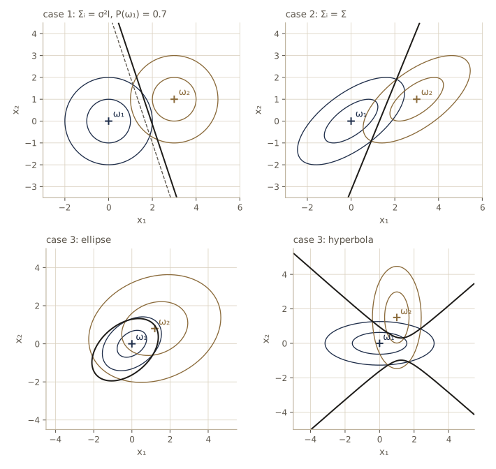
We now set up our own two-class examples in the plane, one per case. In case 1 the priors are unequal, so the boundary should be perpendicular to the line of means but shifted away from the more probable class. In case 2 the boundary should cross the line of means at \(\mathbf{x}_0\) but at a tilt.
mA, mB = np.array([0.0, 0.0]), np.array([3.0, 1.0])
case1 = dict(means=[mA, mB], covs=[np.eye(2), np.eye(2)], priors=[0.7, 0.3])
S_shared = np.array([[1.5, 0.8], [0.8, 1.0]])
case2 = dict(means=[mA, mB], covs=[S_shared, S_shared], priors=[0.5, 0.5])

Sinv_shared = np.linalg.solve(S_shared, np.eye(2))
for name, case, Sinv in [("case 1", case1, np.eye(2)), ("case 2", case2, Sinv_shared)]:
    (W1, w1, w10), (W2, w2, w20) = gaussian_bayes(**case)
    diff = mA - mB
    w = Sinv @ diff                                           # normal of the boundary
    P1, P2 = case["priors"]
    x0 = 0.5 * (mA + mB) - np.log(P1 / P2) / (diff @ Sinv @ diff) * diff
    g0 = g_value(x0, (W1, w1, w10)) - g_value(x0, (W2, w2, w20))
    cos = w @ diff / (np.linalg.norm(w) * np.linalg.norm(diff))
    print(f"{name}: W1 = W2: {np.allclose(W1, W2)};  w = {w};  x0 = {x0}")
    print(f"        g1 - g2 at x0 = {g0[0]:.1e};  "
          f"angle(w, mu1 - mu2) = {np.degrees(np.arccos(cos)):.1f} deg")
move = np.log(0.7 / 0.3) / np.linalg.norm(mA - mB)     # sigma^2 = 1
print(f"case 1: boundary moved {move:.4f} from the midpoint, toward mu_2")
case 1: W1 = W2: True;  w = [-3. -1.];  x0 = [1.7542 0.5847]
        g1 - g2 at x0 = 0.0e+00;  angle(w, mu1 - mu2) = 0.0 deg
case 2: W1 = W2: True;  w = [-2.5581  1.0465];  x0 = [1.5 0.5]
        g1 - g2 at x0 = 0.0e+00;  angle(w, mu1 - mu2) = 40.7 deg
case 1: boundary moved 0.2679 from the midpoint, toward mu_2
In case 1 the normal points along \(\boldsymbol{\mu}_1 - \boldsymbol{\mu}_2\) (angle 0) and \(\mathbf{x}_0\) has moved from the midpoint \((1.5, 0.5)\) toward the less probable class. In case 2 the normal is tilted by the angle shown, as whitening predicts.
For case 3 we build two examples. In the first, class \(\omega_1\) is a tight cloud and \(\omega_2\) a broad one; in the second, the two classes are elongated in perpendicular directions. The eigenvalues of \(\mathbf{W}_1 - \mathbf{W}_2\) tell us which conic each boundary is.
case3_ellipse = dict(means=[mA, np.array([1.2, 0.8])],
                     covs=[np.array([[0.6, 0.2], [0.2, 0.5]]),
                           np.array([[3.0, 0.5], [0.5, 2.0]])],
                     priors=[0.5, 0.5])
case3_hyper = dict(means=[mA, np.array([1.0, 1.5])],
                   covs=[np.diag([2.5, 0.4]), np.diag([0.5, 2.2])],
                   priors=[0.5, 0.5])

def conic_type(W_diff):
    ev = np.linalg.eigvalsh(W_diff)
    if np.any(np.isclose(ev, 0)):
        return "parabola (or degenerate)", ev
    return ("ellipse" if ev[0] * ev[1] > 0 else "hyperbola"), ev

angles = np.linspace(0, 2 * np.pi, 360)
far = 30 * np.column_stack([np.cos(angles), np.sin(angles)])   # a circle of radius 30
for name, case in [("ellipse example", case3_ellipse), ("hyperbola example", case3_hyper)]:
    discs = gaussian_bayes(**case)
    kind, ev = conic_type(discs[0][0] - discs[1][0])
    lab_far = classify(far, discs)
    print(f"{name}: eigenvalues of W1 - W2 = {ev} -> {kind}")
    print(f"    points of the far circle assigned to class 1: {np.sum(lab_far == 0)} of 360")
ellipse example: eigenvalues of W1 - W2 = [-1.1855 -0.4951] -> ellipse
    points of the far circle assigned to class 1: 0 of 360
hyperbola example: eigenvalues of W1 - W2 = [-1.0227  0.8   ] -> hyperbola
    points of the far circle assigned to class 1: 166 of 360
In the first example both eigenvalues are negative, so the boundary is an ellipse: \(\mathcal{R}_1\) is a bounded island, and far from the origin the broad class always wins. In the second, the eigenvalues have opposite signs, the boundary is a hyperbola, and each class wins in two opposite directions far away, so both regions are unbounded. A hyperbola divides the plane into three pieces, so one of the two decision regions consists of two separate parts. The figure shows all four examples.
Error probabilities and integrals
The Bayes rule is the best possible, but how good is it? To answer, we look at how a classifier’s errors arise. Take any dichotomizer, optimal or not, with regions \(\mathcal{R}_1\) and \(\mathcal{R}_2\). An error happens when \(\mathbf{x}\) lands in \(\mathcal{R}_2\) while the class is \(\omega_1\), or in \(\mathcal{R}_1\) while the class is \(\omega_2\). These events are disjoint, so
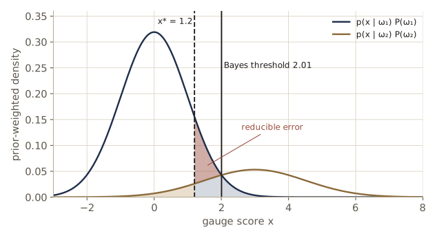
\[\begin{aligned} P(\text{error}) &= P(\mathbf{x} \in \mathcal{R}_2, \omega_1) + P(\mathbf{x} \in \mathcal{R}_1, \omega_2) \\ &= \int_{\mathcal{R}_2} p(\mathbf{x} \mid \omega_1)P(\omega_1)\, d\mathbf{x} + \int_{\mathcal{R}_1} p(\mathbf{x} \mid \omega_2)P(\omega_2)\, d\mathbf{x}. \end{aligned}\]In one dimension with a single threshold \(x^{*}\), the two integrals are the tail of the \(\omega_1\) curve beyond \(x^{*}\) and the tail of the \(\omega_2\) curve before it, both curves weighted by their priors. Moving \(x^{*}\) to the point \(x_B\) where \(p(x \mid \omega_1)P(\omega_1) = p(x \mid \omega_2)P(\omega_2)\) removes a sliver of error between \(x^{*}\) and \(x_B\). That sliver is the reducible error; what remains at \(x_B\) is the Bayes error, which no threshold can remove. In general: wherever \(p(\mathbf{x} \mid \omega_1)P(\omega_1) > p(\mathbf{x} \mid \omega_2)P(\omega_2)\), putting \(\mathbf{x}\) in \(\mathcal{R}_1\) makes the smaller of the two quantities count as the error, which is exactly what the Bayes rule does.
With \(c\) classes there are many more ways to be wrong than right, so it is easier to write the probability of being correct:
\[P(\text{correct}) = \sum_{i=1}^{c} P(\mathbf{x} \in \mathcal{R}_i, \omega_i) = \sum_{i=1}^{c} \int_{\mathcal{R}_i} p(\mathbf{x} \mid \omega_i)P(\omega_i)\, d\mathbf{x}.\]This holds for any partition into regions and any densities. The Bayes rule maximizes it by putting each \(\mathbf{x}\) in the region whose integrand is largest there.
For the inspection problem, take the threshold \(x^{*} = 1.2\) of the minimax rule and compare it with the Bayes threshold for \(P(\omega_1) = 0.8\). The cell computes each error in closed form and the reducible part as the integral of \(\lvert p(x \mid \omega_1)P(\omega_1) - p(x \mid \omega_2)P(\omega_2) \rvert\) between the two thresholds.
def threshold_error(x_star, prior=prior):
    """Error of 'decide omega_2 when x > x_star' (the far-left region is ignored)."""
    return (prior[0] * (1 - ndtr((x_star - mu[0]) / sd[0]))
            + prior[1] * ndtr((x_star - mu[1]) / sd[1]))

x_B = lr_test(np.log(prior[0] / prior[1]))[1]           # the Bayes threshold (right root)
x_star = 1.2
seg = np.linspace(x_star, x_B, 20001)
f = np.exp(class_loglik(seg)) * prior
reducible = np.abs(f[:, 0] - f[:, 1]).sum() * (seg[1] - seg[0])
print(f"x_B = {x_B:.4f}:  error {threshold_error(x_B):.4f}  "
      f"(exact Bayes error, far-left piece included: {error_of_test(np.log(4), 0.8):.4f})")
print(f"x* = {x_star:.4f}:  error {threshold_error(x_star):.4f}")
excess = threshold_error(x_star) - threshold_error(x_B)
print(f"difference {excess:.4f}   reducible-error integral {reducible:.4f}")
x_B = 2.0057:  error 0.0687  (exact Bayes error, far-left piece included: 0.0687)
x* = 1.2000:  error 0.1151
difference 0.0464   reducible-error integral 0.0464
The minimax threshold, used when 80% of parts are good, makes about 1.7 times as many errors as necessary, and the whole excess is the reducible-error sliver between the two thresholds. (The far-left piece of the Bayes region changes the Bayes error only in the eighth decimal place.)
In more than one dimension the error integral runs over curved regions, and closed forms are rare. In two dimensions we can still integrate \(\min_j p(\mathbf{x} \mid \omega_j)P(\omega_j)\) on a grid, and Monte Carlo works in any dimension: draw labeled samples, classify them with the Bayes rule, and count mistakes. The Monte Carlo estimate has standard error \(\sqrt{\hat{P}(1 - \hat{P})/n}\), which we print alongside.
def bayes_error_grid(case, lim=9.0, n=801):
    """Integral of min_j p(x | w_j) P(w_j) over a square grid (two classes, two dimensions)."""
    g = np.linspace(-lim, lim, n)
    G = np.array(np.meshgrid(g, g)).reshape(2, -1).T
    joint = np.column_stack([np.exp(log_gauss(G, m, S)) * P
                             for m, S, P in zip(case["means"], case["covs"], case["priors"])])
    return joint.min(axis=1).sum() * (g[1] - g[0]) ** 2

def bayes_error_mc(case, n, gen):
    """Sample classes from the priors, then features; return the error rate and its std. error."""
    labels = gen.choice(len(case["priors"]), size=n, p=case["priors"])
    X = np.empty((n, 2))
    for j, (m, S) in enumerate(zip(case["means"], case["covs"])):
        X[labels == j] = sample_gauss(np.sum(labels == j), m, S, gen)
    err = np.mean(classify(X, gaussian_bayes(**case)) != labels)
    return err, np.sqrt(err * (1 - err) / n)

rng_mc = np.random.default_rng(2)
for name, case in [("case 1", case1), ("case 2", case2),
                   ("case 3 ellipse", case3_ellipse), ("case 3 hyperbola", case3_hyper)]:
    e_mc, se = bayes_error_mc(case, 200000, rng_mc)
    print(f"{name:17s} grid integral {bayes_error_grid(case):.4f}   "
          f"Monte Carlo {e_mc:.4f} +/- {se:.4f}")
case 1            grid integral 0.0509   Monte Carlo 0.0507 +/- 0.0005
case 2            grid integral 0.0990   Monte Carlo 0.0991 +/- 0.0007
case 3 ellipse    grid integral 0.1894   Monte Carlo 0.1899 +/- 0.0009
case 3 hyperbola  grid integral 0.1708   Monte Carlo 0.1702 +/- 0.0008
The two estimates agree within the Monte Carlo standard error in every case.
Note. The Bayes error is a property of the features and the class distributions, not of any classifier. Adding a feature can never raise it, since the Bayes rule for the larger feature set could always ignore the new feature. In practice more features can still hurt, because the densities must be estimated from a limited number of samples; module 03 takes up this problem of dimensionality.
For cases 1 and 2 an exact answer exists: with a common covariance the discriminant \(g(\mathbf{x})\) is linear, so it is itself normal under each class, and the error is a combination of two values of \(\Phi\) (Exercise 5). With unequal covariances no such shortcut exists, which motivates the bounds of the next section.
Error bounds for normal densities
For Gaussian classes in many dimensions, the error integral over quadric regions has no closed form, and grids become impossible beyond a few dimensions. For two classes, though, we can bound the error without ever finding the decision regions.
The Chernoff bound
The bound rests on an elementary inequality: for \(a, b \ge 0\) and \(0 \le \beta \le 1\),
\[\min[a, b] \le a^{\beta} b^{1-\beta}.\]To see it, suppose \(a \ge b\) (the other case is symmetric). Then \(a^{\beta}b^{1-\beta} = b\,(a/b)^{\beta} \ge b = \min[a, b]\), because \((a/b)^{\beta} \ge 1\). Apply it inside the Bayes error integral, \(P(\text{error}) = \int \min[P(\omega_1)p(\mathbf{x} \mid \omega_1), P(\omega_2)p(\mathbf{x} \mid \omega_2)]\, d\mathbf{x}\):
\[P(\text{error}) \le P^{\beta}(\omega_1)\, P^{1-\beta}(\omega_2) \int p^{\beta}(\mathbf{x} \mid \omega_1)\, p^{1-\beta}(\mathbf{x} \mid \omega_2)\, d\mathbf{x}, \qquad 0 \le \beta \le 1.\]The integral now runs over the whole space; the decision regions have disappeared. For normal densities it can be done in closed form. The product \(p^{\beta}(\mathbf{x} \mid \omega_1)\,p^{1-\beta}(\mathbf{x} \mid \omega_2)\) is the exponential of a quadratic in \(\mathbf{x}\), an unnormalized Gaussian with inverse covariance \(\beta\boldsymbol{\Sigma}_1^{-1} + (1-\beta)\boldsymbol{\Sigma}_2^{-1}\); completing the square and integrating (DHS Problem 36 walks through the steps) gives \(e^{-k(\beta)}\) with
\[k(\beta) = \frac{\beta(1-\beta)}{2}(\boldsymbol{\mu}_2 - \boldsymbol{\mu}_1)^{t}\big[(1-\beta)\boldsymbol{\Sigma}_1 + \beta\boldsymbol{\Sigma}_2\big]^{-1}(\boldsymbol{\mu}_2 - \boldsymbol{\mu}_1) + \frac{1}{2}\ln\frac{\lvert (1-\beta)\boldsymbol{\Sigma}_1 + \beta\boldsymbol{\Sigma}_2 \rvert}{\lvert \boldsymbol{\Sigma}_1 \rvert^{1-\beta}\lvert \boldsymbol{\Sigma}_2 \rvert^{\beta}}.\]The first term measures how far apart the means are, the second how different the covariances are; both are zero when the classes coincide. The Chernoff bound is the smallest of these bounds, found by minimizing \(P^{\beta}(\omega_1)P^{1-\beta}(\omega_2)e^{-k(\beta)}\) over \(\beta\). That is a one-dimensional search however large \(d\) is. It is also well behaved: the logarithm of the bound is a convex function of \(\beta\) (the log of \(\int p_2\,(p_1/p_2)^{\beta}\) is convex, as a log of a sum of exponentials in \(\beta\)), so a golden-section search finds the minimum. At the ends, \(\beta \to 0\) and \(\beta \to 1\), the bound tends to \(P(\omega_2)\) and \(P(\omega_1)\), the error of a rule that ignores \(\mathbf{x}\); the useful values are in between.
We first check the closed form of \(e^{-k(\beta)}\) against direct numerical integration, in one dimension (the inspection problem) and in two (the case 3 ellipse example).
def chernoff_k(beta, m1, S1, m2, S2):
    """k(beta) for Gaussian classes N(m1, S1), N(m2, S2)."""
    S1, S2 = np.atleast_2d(S1), np.atleast_2d(S2)
    D = np.atleast_1d(m2 - m1)
    S_mix = (1 - beta) * S1 + beta * S2
    quad = D @ np.linalg.solve(S_mix, D)
    logdet = lambda A: np.linalg.slogdet(A)[1]
    log_ratio = logdet(S_mix) - (1 - beta) * logdet(S1) - beta * logdet(S2)
    return 0.5 * beta * (1 - beta) * quad + 0.5 * log_ratio

beta = 0.3
# one dimension: integrate p1^beta p2^(1-beta) on x_grid
lp = class_loglik(x_grid)
num_1d = np.exp(beta * lp[:, 0] + (1 - beta) * lp[:, 1]).sum() * dx
k_1d = chernoff_k(beta, mu[0], sd[0]**2, mu[1], sd[1]**2)
print(f"1-D: numerical {num_1d:.6f}   exp(-k) {np.exp(-k_1d):.6f}")
# two dimensions
g2 = np.linspace(-10, 10, 801)
G2 = np.array(np.meshgrid(g2, g2)).reshape(2, -1).T
(mE1, mE2), (SE1, SE2) = case3_ellipse["means"], case3_ellipse["covs"]
log_prod = beta * log_gauss(G2, mE1, SE1) + (1 - beta) * log_gauss(G2, mE2, SE2)
num_2d = np.exp(log_prod).sum() * (g2[1] - g2[0])**2
k_2d = chernoff_k(beta, mE1, SE1, mE2, SE2)
print(f"2-D: numerical {num_2d:.6f}   exp(-k) {np.exp(-k_2d):.6f}")
1-D: numerical 0.484392   exp(-k) 0.484392
2-D: numerical 0.646499   exp(-k) 0.646499
Now the search. The golden-section method keeps a bracket \([l, u]\) and two interior points that divide it in the golden ratio; each step discards the part of the bracket beyond the worse point and reuses the other point, shrinking the bracket by a factor of about 0.618.
def golden_min(f, lo, hi, tol=1e-8):
    """Minimize a unimodal f on [lo, hi] by golden-section search."""
    r = (np.sqrt(5) - 1) / 2
    a, b = hi - r * (hi - lo), lo + r * (hi - lo)
    fa, fb = f(a), f(b)
    while hi - lo > tol:
        if fa < fb:
            hi, b, fb = b, a, fa
            a = hi - r * (hi - lo); fa = f(a)
        else:
            lo, a, fa = a, b, fb
            b = lo + r * (hi - lo); fb = f(b)
    return 0.5 * (lo + hi)

def error_bounds(m1, S1, m2, S2, P1):
    bound = lambda b: P1**b * (1 - P1)**(1 - b) * np.exp(-chernoff_k(b, m1, S1, m2, S2))
    b_star = golden_min(lambda b: np.log(bound(b)), 1e-6, 1 - 1e-6)
    return b_star, bound(b_star), bound(0.5)

(mH1, mH2), (SH1, SH2) = case3_hyper["means"], case3_hyper["covs"]
problems = [   # name, (m1, S1, m2, S2, P1), Bayes error
    ("inspection, 1-D", (mu[0], sd[0]**2, mu[1], sd[1]**2, prior[0]),
     error_of_test(np.log(4), 0.8)),
    ("case 2 (shared cov.)", (mA, S_shared, mB, S_shared, 0.5), bayes_error_grid(case2)),
    ("case 3 ellipse", (mE1, SE1, mE2, SE2, 0.5), bayes_error_grid(case3_ellipse)),
    ("case 3 hyperbola", (mH1, SH1, mH2, SH2, 0.5), bayes_error_grid(case3_hyper)),
]
print("problem                 beta*   Chernoff   Bhattacharyya   Bayes error")
for name, args, err in problems:
    b_star, ch, bh = error_bounds(*args)
    print(f"{name:22s}  {b_star:.3f}    {ch:.4f}       {bh:.4f}        {err:.4f}")
problem                 beta*   Chernoff   Bhattacharyya   Bayes error
inspection, 1-D         0.228    0.1433       0.1923        0.0687
case 2 (shared cov.)    0.500    0.2184       0.2184        0.0990
case 3 ellipse          0.358    0.3211       0.3315        0.1894
case 3 hyperbola        0.435    0.2699       0.2717        0.1708
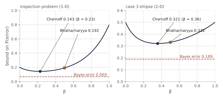
Every bound lies above the true error, as it must. For the inspection problem the unequal priors pull the best exponent far from one half, to \(\beta^{*} \approx 0.23\), and the Chernoff bound (0.143) is much tighter than the value at \(\beta = 1/2\) (0.192). With a shared covariance and equal priors, \(k(\beta)\) is symmetric about one half and \(\beta^{*} = 1/2\) exactly. In all four problems the best bound is between about 1.6 and 2.2 times the Bayes error: not tight, but available in closed form in any dimension.
The Bhattacharyya bound
Skipping the search and simply setting \(\beta = 1/2\) gives the Bhattacharyya bound,
\[P(\text{error}) \le \sqrt{P(\omega_1)P(\omega_2)} \int \sqrt{p(\mathbf{x} \mid \omega_1)\,p(\mathbf{x} \mid \omega_2)}\, d\mathbf{x} = \sqrt{P(\omega_1)P(\omega_2)}\; e^{-k(1/2)},\]where for Gaussian classes
\[k(1/2) = \frac{1}{8}(\boldsymbol{\mu}_2 - \boldsymbol{\mu}_1)^{t}\left[\frac{\boldsymbol{\Sigma}_1 + \boldsymbol{\Sigma}_2}{2}\right]^{-1}(\boldsymbol{\mu}_2 - \boldsymbol{\mu}_1) + \frac{1}{2}\ln\frac{\big\lvert \frac{\boldsymbol{\Sigma}_1 + \boldsymbol{\Sigma}_2}{2} \big\rvert}{\sqrt{\lvert \boldsymbol{\Sigma}_1 \rvert \lvert \boldsymbol{\Sigma}_2 \rvert}}.\]The quantity \(k(1/2)\) is the Bhattacharyya distance between the two densities. It is never tighter than the Chernoff bound, but it is simpler, symmetric in the two classes, and often almost as good, as the table shows for the equal-prior problems. It is widely used as a measure of how separable two classes are, for example to compare candidate feature sets. The bounds remain valid for non-Gaussian densities if the integral is computed for those densities; what is specific to Gaussians is the closed form for \(k(\beta)\), and plugging Gaussian formulas into markedly non-Gaussian data gives numbers that need not bound anything.
Signal detection theory and ROC curves
Another way of summarizing how separable two classes are comes from the study of detectors: a radar deciding whether a faint echo is present, or a listener deciding whether a faint tone was played. Inside the detector is an internal signal \(x\). Without the external signal it is \(N(\mu_1, \sigma^2)\); with it, \(N(\mu_2, \sigma^2)\), same variance, larger mean. The detector says “present” when \(x > x^{*}\) for some threshold \(x^{*}\) we cannot see. The discriminability
\[d' = \frac{\lvert \mu_2 - \mu_1 \rvert}{\sigma}\]measures how far apart the two densities are in units of their spread. It depends on the signal strength and the noise, not on where the threshold is set.
Each trial ends in one of four outcomes. With the signal present, answering “present” is a hit and “absent” a miss; with the signal absent, “present” is a false alarm and “absent” a correct rejection. From many trials we can estimate the hit rate \(H = P(x > x^{*} \mid \omega_2)\) and the false-alarm rate \(F = P(x > x^{*} \mid \omega_1)\). Remarkably, these two numbers are enough to recover \(d'\) without knowing \(\mu_1\), \(\mu_2\), \(\sigma\), or \(x^{*}\). Standardizing,
\[F = 1 - \Phi\left(\frac{x^{*} - \mu_1}{\sigma}\right), \qquad H = 1 - \Phi\left(\frac{x^{*} - \mu_2}{\sigma}\right),\]so \(\Phi^{-1}(F) = (\mu_1 - x^{*})/\sigma\) and \(\Phi^{-1}(H) = (\mu_2 - x^{*})/\sigma\). Subtracting,
\[d' = \Phi^{-1}(H) - \Phi^{-1}(F),\]and \(-\Phi^{-1}(F)\) tells us where the threshold sits, in units of \(\sigma\) above the noise mean. This separates two things that a single error rate mixes up: the discriminability of the detector, fixed by physics, and its decision bias, the threshold, which reflects the costs the observer has in mind and can change. If the Gaussian model holds, \(d'\) also gives the best achievable error: with equal priors the Bayes threshold is the midpoint, and \(P(\text{error}) = \Phi(-d'/2)\).
Let us run such an experiment. The detector’s parameters are hidden inside the simulation; the “experimenter” sees only which trials were answered “present”.
rng_sd = np.random.default_rng(7)
mu_noise, mu_signal, sig, x_thr = 0.0, 1.3, 1.0, 0.9     # hidden: d' = 1.3
n_trials = 2000
x_noise = rng_sd.normal(mu_noise, sig, n_trials)          # signal absent (omega_1)
x_signal = rng_sd.normal(mu_signal, sig, n_trials)        # signal present (omega_2)
F_hat, H_hat = np.mean(x_noise > x_thr), np.mean(x_signal > x_thr)

d_hat = ndtri(H_hat) - ndtri(F_hat)
print(f"false-alarm rate {F_hat:.4f}, hit rate {H_hat:.4f}")
print(f"estimated d' = {d_hat:.3f} (true 1.3);  threshold at {-ndtri(F_hat):.3f} "
      f"sigma above the noise mean (true 0.9)")
print(f"implied Bayes error with equal priors: {ndtr(-d_hat / 2):.4f} "
      f"(true {ndtr(-1.3 / 2):.4f})")
false-alarm rate 0.1705, hit rate 0.6550
estimated d' = 1.351 (true 1.3);  threshold at 0.952 sigma above the noise mean (true 0.9)
implied Bayes error with equal priors: 0.2497 (true 0.2578)
With 2000 trials of each kind, the recovered \(d'\) and threshold are within about 0.05 of the hidden values, and the implied Bayes error is close to the true one.
If we keep the densities fixed and slide the threshold, the pair \((F, H)\) moves along a curve from \((1, 1)\) (threshold far left: always “present”) to \((0, 0)\) (always “absent”). This curve is the receiver operating characteristic, or ROC curve. For the equal-variance model, eliminating the threshold from the two equations above gives it explicitly: \(H = \Phi\big(d' + \Phi^{-1}(F)\big)\). Every \(d'\) has its own curve; \(d' = 0\) is the diagonal \(H = F\) (a useless detector), and larger \(d'\) bows the curve toward the corner \((0, 1)\). Exactly one of these curves passes through any measured point with \(0 < F, H < 1\), which is another way of saying that \((F, H)\) determines \(d'\).
A common one-number summary is the area under the ROC curve (AUC). It has a direct meaning: the AUC is the probability that a randomly chosen signal trial produces a larger \(x\) than a randomly chosen noise trial. For the equal-variance model the difference of the two is \(N(\mu_2 - \mu_1, 2\sigma^2)\), so AUC \(= \Phi(d'/\sqrt{2})\). The cell computes it three ways: by integrating the ROC curve, from the formula, and from the simulated trials by counting correctly ordered pairs.
def roc_equal_variance(F, d_prime):
    return ndtr(d_prime + ndtri(F))

F_grid = np.linspace(0, 1, 20001)
H_grid = roc_equal_variance(F_grid, 1.3)
auc_trapz = np.sum(0.5 * (H_grid[1:] + H_grid[:-1]) * np.diff(F_grid))
# empirical: fraction of (signal, noise) pairs ordered correctly, via ranks
ranks = np.searchsorted(np.sort(x_noise), x_signal)   # noise trials below each signal trial
auc_emp = ranks.mean() / n_trials
print(f"AUC: trapezoid {auc_trapz:.4f}   formula Phi(d'/sqrt 2) {ndtr(1.3 / np.sqrt(2)):.4f}   "
      f"from the {n_trials} + {n_trials} trials {auc_emp:.4f}")
AUC: trapezoid 0.8210 formula Phi(d'/sqrt 2) 0.8210 from the 2000 + 2000 trials 0.8310
The first two agree to four digits. The estimate from the trials is about 0.01 higher, a typical sampling fluctuation for 2000 trials per class (its standard error is roughly 0.007).
The same picture works for any two-class problem, in any dimension, with any densities: fix a family of decision rules indexed by one control parameter, usually a threshold on a score, and plot hit rate against false-alarm rate as the parameter varies. The result is called an operating characteristic. The best possible family is the likelihood-ratio test with a varying threshold, since by the Neyman–Pearson lemma it gives the highest hit rate at every false-alarm rate. When the two classes have different variances the curve is no longer symmetric about the anti-diagonal, and no single \(d'\) describes it: the formula above gives a different value at different points.
The inspection problem is such a case. Its ROC comes straight from lr_test, and every rule of this module is a point on it. Once the ROC is known, choosing a rule for new costs is a one-line search: the risk is linear in \((F, H)\),
so we pick the point of the curve that minimizes it. Its lines of constant risk have slope \((\lambda_{21} - \lambda_{11})P(\omega_1)/[(\lambda_{12} - \lambda_{22})P(\omega_2)]\), and the best point is where the ROC has that slope, the likelihood-ratio threshold of the Bayes rule once more.
ts = np.linspace(-8, 12, 4001)
roc = np.array([lr_test(t)[2:] for t in ts])               # columns: false alarm, hit
FA_roc, H_roc = roc[:, 0], roc[:, 1]
order = np.argsort(FA_roc)
auc_insp = np.sum(0.5 * (H_roc[order][1:] + H_roc[order][:-1]) * np.diff(FA_roc[order]))
print(f"inspection problem: AUC = {auc_insp:.4f}")
for F0 in [0.05, 0.30]:
    H0 = np.interp(F0, FA_roc[order], H_roc[order])
    print(f"d' read off the ROC at F = {F0:.2f}: {ndtri(H0) - ndtri(F0):.3f}")

# a new loss: shipping a defect now costs 20; choose the operating point from the ROC table
Lam_20 = np.array([[0.0, 20.0], [1.0, 0.0]])
risk_roc = prior[0] * (Lam_20[0, 0] + (Lam_20[1, 0] - Lam_20[0, 0]) * FA_roc) + \
           prior[1] * (Lam_20[1, 1] + (Lam_20[0, 1] - Lam_20[1, 1]) * (1 - H_roc))
k = risk_roc.argmin()
print(f"best point on the ROC: F = {FA_roc[k]:.4f}, H = {H_roc[k]:.4f}, "
      f"risk {risk_roc[k]:.4f}, at t = {ts[k]:.3f}")
print(f"Bayes rule from the formula: t = {bayes_log_threshold(Lam_20):.3f}, "
      f"risk {bayes_risk_of_test(bayes_log_threshold(Lam_20), Lam_20):.4f}")
inspection problem: AUC = 0.9520
d' read off the ROC at F = 0.05: 2.548
d' read off the ROC at F = 0.30: 2.175
best point on the ROC: F = 0.2958, H = 0.9497, risk 0.4377, at t = -1.610
Bayes rule from the formula: t = -1.609, risk 0.4377
The two readings of \(d'\) differ, confirming that the unequal-variance ROC is not one of the equal-variance family. The search along the ROC recovers the Bayes threshold for the new costs, to the resolution of the grid of thresholds.
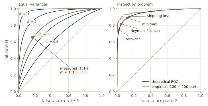
Discrete features
So far \(\mathbf{x}\) has been a point of \(\mathbb{R}^d\). In many problems the features take only a finite set of values: yes/no answers, counts, categories. Then \(\mathbf{x}\) can take only values \(\mathbf{v}_1, \dots, \mathbf{v}_m\), class-conditional densities become probabilities \(P(\mathbf{x} \mid \omega_j)\), and integrals become sums. Bayes’ formula reads
\[P(\omega_j \mid \mathbf{x}) = \frac{P(\mathbf{x} \mid \omega_j)\,P(\omega_j)}{P(\mathbf{x})}, \qquad P(\mathbf{x}) = \sum_{k=1}^{c} P(\mathbf{x} \mid \omega_k)\,P(\omega_k),\]and nothing else changes: the conditional risk is defined as before, the Bayes rule takes \(\alpha^{*} = \arg\min_i R(\alpha_i \mid \mathbf{x})\), and the minimum-error discriminants are those of the section on discriminant functions with \(P\) in place of \(p\).
Independent binary features
The most important discrete model has \(d\) binary features, \(x_i \in \{0, 1\}\), that are conditionally independent given the class. For two classes, write
\[p_i = P(x_i = 1 \mid \omega_1), \qquad q_i = P(x_i = 1 \mid \omega_2).\]For our inspection line, imagine four quick yes/no checks, each of which may raise a flag (\(x_i = 1\)). A single binary feature has probability \(p_i^{x_i}(1 - p_i)^{1 - x_i}\), which is \(p_i\) when \(x_i = 1\) and \(1 - p_i\) when \(x_i = 0\). Independence makes the class-conditional probability a product:
\[P(\mathbf{x} \mid \omega_1) = \prod_{i=1}^{d} p_i^{x_i}(1 - p_i)^{1 - x_i}, \qquad P(\mathbf{x} \mid \omega_2) = \prod_{i=1}^{d} q_i^{x_i}(1 - q_i)^{1 - x_i}.\]Take the log likelihood ratio plus the log prior ratio, the dichotomizer from before:
\[g(\mathbf{x}) = \sum_{i=1}^{d}\left[x_i \ln\frac{p_i}{q_i} + (1 - x_i)\ln\frac{1 - p_i}{1 - q_i}\right] + \ln\frac{P(\omega_1)}{P(\omega_2)}.\]Collecting the terms that multiply \(x_i\) shows that \(g\) is linear in the features:
\[g(\mathbf{x}) = \sum_{i=1}^{d} w_i x_i + w_0, \qquad w_i = \ln\frac{p_i(1 - q_i)}{q_i(1 - p_i)}, \qquad w_0 = \sum_{i=1}^{d}\ln\frac{1 - p_i}{1 - q_i} + \ln\frac{P(\omega_1)}{P(\omega_2)},\]and we decide \(\omega_1\) when \(g(\mathbf{x}) > 0\). The weights have a clear reading. If \(p_i = q_i\) the feature carries no information and \(w_i = 0\). If \(p_i > q_i\), a 1 in feature \(i\) is more common under \(\omega_1\), \(w_i > 0\), and a 1 adds \(w_i\) votes for \(\omega_1\); for fixed \(q_i\) the vote grows with \(p_i\). If \(p_i < q_i\), a 1 votes for \(\omega_2\). The priors enter only through \(w_0\). Geometrically, the \(2^d\) possible vectors are the corners of a hypercube, and \(g(\mathbf{x}) = 0\) is a hyperplane that separates the corners assigned to \(\omega_1\) from the rest.
In our checks, good parts (\(\omega_1\)) rarely raise flags 1 and 2, check 3 flags both classes equally often, and check 4 is a cosmetic check that flags good parts more often than defective ones. The cell computes the weights, compares the linear rule with brute-force posteriors on all 16 corners, and computes the exact Bayes error as a finite sum, checked by Monte Carlo.
p_flag = np.array([0.05, 0.20, 0.30, 0.40])     # P(x_i = 1 | omega_1): good parts
q_flag = np.array([0.50, 0.70, 0.30, 0.20])     # P(x_i = 1 | omega_2): defective parts

w_bin = np.log(p_flag * (1 - q_flag) / (q_flag * (1 - p_flag)))
w0_bin = np.log((1 - p_flag) / (1 - q_flag)).sum() + np.log(prior[0] / prior[1])
print("weights w_i =", w_bin, f"  w_0 = {w0_bin:.4f}")

corners = np.array(list(product([0, 1], repeat=4)))                # all 16 feature vectors
Px1 = np.prod(p_flag**corners * (1 - p_flag)**(1 - corners), axis=1)
Px2 = np.prod(q_flag**corners * (1 - q_flag)**(1 - corners), axis=1)
post_good = Px1 * prior[0] / (Px1 * prior[0] + Px2 * prior[1])      # brute-force posterior
g_bin = corners @ w_bin + w0_bin
log_odds = np.log(post_good / (1 - post_good))
print(f"g(x) equals the log posterior odds: {np.allclose(g_bin, log_odds)}")
print("corners decided 'defective':", ["".join(map(str, c)) for c in corners[g_bin < 0]])

err_exact = np.minimum(Px1 * prior[0], Px2 * prior[1]).sum()
rng_b = np.random.default_rng(11)
lab = rng_b.random(200000) < prior[1]                               # True = defective
Xb = (rng_b.random((200000, 4)) < np.where(lab[:, None], q_flag, p_flag)).astype(int)
err_mc = np.mean((Xb @ w_bin + w0_bin < 0) != lab)
print(f"Bayes error: exact sum {err_exact:.4f}   Monte Carlo {err_mc:.4f}")
weights w_i = [-2.9444 -2.2336  0.      0.9808]   w_0 = 2.7213
g(x) equals the log posterior odds: True
corners decided 'defective': ['1000', '1010', '1100', '1101', '1110', '1111']
Bayes error: exact sum 0.1332   Monte Carlo 0.1336
The linear discriminant reproduces the log posterior odds exactly, as the derivation says. The weight of check 3 is zero, and check 4 has a positive weight: a flag there is evidence of a good part. Reading the list of corners: a flag on check 1 makes the part look defective unless check 4 also flags it, flags on checks 1 and 2 together always do, and a flag on check 2 without one on check 1 never does.
The independence assumption is what made the classifier linear. With dependent binary features the log likelihood ratio contains products such as \(x_i x_j\), and the classifier becomes more complicated. Assuming conditional independence even when it is not exactly true gives the naive Bayes classifier, which often works well in practice; Intro to ML, module 04 fits it to data, and in module 03 we will estimate the \(p_i\) and \(q_i\) from samples.
Missing and noisy features
A Bayes classifier designed for complete, clean measurements may meet patterns where a feature is missing (a sensor failed, part of an object was hidden) or was measured with extra noise. If we know how the damage happened, the Bayes rule tells us what to do: work out the posterior given what we actually observed.
Missing features
Split the feature vector into the good features \(\mathbf{x}_g\), which we observed, and the bad ones \(\mathbf{x}_b\), which are missing. The posterior given only the good features follows from the sum rule, integrating the bad features out of the joint density:
\[P(\omega_i \mid \mathbf{x}_g) = \frac{p(\omega_i, \mathbf{x}_g)}{p(\mathbf{x}_g)} = \frac{\int p(\omega_i, \mathbf{x}_g, \mathbf{x}_b)\, d\mathbf{x}_b}{p(\mathbf{x}_g)} = \frac{\int g_i(\mathbf{x})\, p(\mathbf{x})\, d\mathbf{x}_b}{\int p(\mathbf{x})\, d\mathbf{x}_b},\]where \(g_i(\mathbf{x}) = P(\omega_i \mid \mathbf{x}_g, \mathbf{x}_b)\) is the full-feature posterior. The integrated density is a marginal, and we say the bad features have been marginalized out. The last form says: average the full-feature posterior over the values the missing features could have taken, weighting each by how probable it is. Equivalently, \(P(\omega_i \mid \mathbf{x}_g) \propto p(\mathbf{x}_g \mid \omega_i)P(\omega_i)\) with the marginal class-conditional density. For Gaussian classes that marginal is easy: keep the entries of \(\boldsymbol{\mu}_i\) and the rows and columns of \(\boldsymbol{\Sigma}_i\) that belong to \(\mathbf{x}_g\).
A tempting shortcut is to fill in the missing feature with its average value over all classes and classify as usual. The next example shows why that is wrong. Three equally likely classes live in the plane; class \(\omega_1\) sits far to the left and is the only class centered at \(x_2 = 1.2\). A pattern arrives with \(x_1\) missing and \(x_2 = 1.2\).
means_m = [np.array([-3.0, 1.2]), np.array([0.0, 0.0]), np.array([3.0, 0.0])]
covs_m = [np.diag([1.0, 0.5]), np.eye(2), np.eye(2)]
priors_m = np.array([1, 1, 1]) / 3
discs_m = gaussian_bayes(means_m, covs_m, priors_m)

def posterior_full(X):
    X = np.atleast_2d(X)
    a = np.column_stack([log_gauss(X, m, S) for m, S in zip(means_m, covs_m)]) + np.log(priors_m)
    return np.exp(a - logsumexp(a, axis=1, keepdims=True))

def posterior_x2_only(x2):
    """Marginalize x1: use the x2 entries of each mean and covariance."""
    a = np.array([log_normal_1d(x2, m[1], np.sqrt(S[1, 1])) for m, S in zip(means_m, covs_m)])
    a = a + np.log(priors_m)
    return np.exp(a - logsumexp(a))

x2_obs = 1.2
x1_mean = sum(P * m[0] for P, m in zip(priors_m, means_m))    # average x1 over all classes
print("mean imputation, x1 =", x1_mean, "-> posterior", posterior_full([x1_mean, x2_obs])[0])
print("marginalizing x1          -> posterior", posterior_x2_only(x2_obs))

# the same marginal by integrating the full-feature posterior against p(x1, x2) over x1
t1 = np.linspace(-12, 12, 24001)
pts = np.column_stack([t1, np.full_like(t1, x2_obs)])
p_x = sum(P * np.exp(log_gauss(pts, m, S)) for P, m, S in zip(priors_m, means_m, covs_m))
num = (posterior_full(pts) * p_x[:, None]).sum(axis=0) / p_x.sum()
print("integral of g_i(x) p(x) dx1 / integral of p(x) dx1:", num)
mean imputation, x1 = 0.0 -> posterior [0.0309 0.9584 0.0106]
marginalizing x1          -> posterior [0.5923 0.2039 0.2039]
integral of g_i(x) p(x) dx1 / integral of p(x) dx1: [0.5923 0.2039 0.2039]
Imputing the mean places the pattern at \((0, 1.2)\), right next to \(\omega_2\), and the classifier confidently says \(\omega_2\). But among the three classes only \(\omega_1\) often produces \(x_2 = 1.2\), and the marginal posterior correctly favors it. Averaging over the possible values of \(x_1\) is not the same as plugging in the average value. The integral check confirms the marginal formula.
To see what this costs on average, delete \(x_1\) from a large test set and compare the two strategies, with the full-feature Bayes rule as a reference.
rng_m = np.random.default_rng(5)
n_m = 30000
lab_m = rng_m.choice(3, size=n_m, p=priors_m)
X_m = np.empty((n_m, 2))
for j in range(3):
    X_m[lab_m == j] = sample_gauss(np.sum(lab_m == j), means_m[j], covs_m[j], rng_m)

pred_full = classify(X_m, discs_m)
pred_impute = classify(np.column_stack([np.full(n_m, x1_mean), X_m[:, 1]]), discs_m)
a_marg = np.column_stack([log_normal_1d(X_m[:, 1], m[1], np.sqrt(S[1, 1]))
                          for m, S in zip(means_m, covs_m)])
pred_marg = (a_marg + np.log(priors_m)).argmax(axis=1)
for name, pred in [("both features", pred_full), ("x1 missing, mean imputed", pred_impute),
                   ("x1 missing, marginalized", pred_marg)]:
    print(f"{name:26s} error rate {np.mean(pred != lab_m):.4f}")
both features              error rate 0.0786
x1 missing, mean imputed   error rate 0.6690
x1 missing, marginalized   error rate 0.4900
Mean imputation does no better than guessing among three classes. Losing \(x_1\) costs a lot whatever we do, since \(x_1\) is the feature that separates \(\omega_2\) from \(\omega_3\). But marginalizing is clearly better than imputing the mean, and it is the best any rule can do with \(x_2\) alone, because it is the Bayes rule for that problem. When whole training samples have missing values, the same marginalization idea leads to the EM algorithm of module 03.
Noisy features
Now suppose feature \(\mathbf{x}_b\) was measured, but through extra noise: we observe \(\mathbf{x}_b\) while the true value is \(\mathbf{x}_t\), and we know the noise model \(p(\mathbf{x}_b \mid \mathbf{x}_t)\). Assume that once the true value is known, the noisy reading adds nothing about the class or about \(\mathbf{x}_g\). We integrate over the unknown true value:
\[P(\omega_i \mid \mathbf{x}_g, \mathbf{x}_b) = \frac{\int p(\omega_i, \mathbf{x}_g, \mathbf{x}_b, \mathbf{x}_t)\, d\mathbf{x}_t}{p(\mathbf{x}_g, \mathbf{x}_b)}.\]By the chain rule, \(p(\omega_i, \mathbf{x}_g, \mathbf{x}_b, \mathbf{x}_t) = P(\omega_i \mid \mathbf{x}_g, \mathbf{x}_b, \mathbf{x}_t)\,p(\mathbf{x}_b \mid \mathbf{x}_g, \mathbf{x}_t)\,p(\mathbf{x}_g, \mathbf{x}_t)\), and the independence assumption reduces the first two factors to \(P(\omega_i \mid \mathbf{x}_g, \mathbf{x}_t)\) and \(p(\mathbf{x}_b \mid \mathbf{x}_t)\). With \(\mathbf{x} = (\mathbf{x}_g, \mathbf{x}_t)\),
\[P(\omega_i \mid \mathbf{x}_g, \mathbf{x}_b) = \frac{\int g_i(\mathbf{x})\, p(\mathbf{x})\, p(\mathbf{x}_b \mid \mathbf{x}_t)\, d\mathbf{x}_t}{\int p(\mathbf{x})\, p(\mathbf{x}_b \mid \mathbf{x}_t)\, d\mathbf{x}_t}.\]This is the missing-feature formula with the integral weighted by the noise model. If the noise is so large that \(p(\mathbf{x}_b \mid \mathbf{x}_t)\) is flat in \(\mathbf{x}_t\), it cancels and we are back to a missing feature; if the noise vanishes, it becomes a spike at \(\mathbf{x}_t = \mathbf{x}_b\) and we recover the full-feature posterior. For Gaussian classes and additive Gaussian noise \(\mathbf{x}_b = \mathbf{x}_t + \boldsymbol{\epsilon}\), \(\boldsymbol{\epsilon} \sim N(\mathbf{0}, s^2\mathbf{I})\), the observed vector is again Gaussian, with the noise variance added to the \(\mathbf{x}_b\) block of each \(\boldsymbol{\Sigma}_i\). The cell uses this to follow a pattern at \((-1, 1.2)\) as the noise on \(x_1\) grows, and checks one noise level against the integral.
x_obs = np.array([-1.0, 1.2])

def posterior_noisy(x, s):
    """x1 observed through N(0, s^2) noise: add s^2 to the (1,1) entry of each covariance."""
    a = np.array([log_gauss(x, m, S + np.diag([s**2, 0.0]))[0] for m, S in zip(means_m, covs_m)])
    a = a + np.log(priors_m)
    return np.exp(a - logsumexp(a))

print("   s     P(w1)    P(w2)    P(w3)")
for s in [0.0, 0.5, 1.0, 2.0, 5.0, 100.0]:
    print(f"{s:6.1f}  ", posterior_noisy(x_obs, s))
print("x1 missing", posterior_x2_only(x_obs[1]))

# check s = 1 against the integral over the true value x_t
s = 1.0
pts = np.column_stack([t1, np.full_like(t1, x_obs[1])])      # (x_t, x2)
p_x = sum(P * np.exp(log_gauss(pts, m, S)) for P, m, S in zip(priors_m, means_m, covs_m))
noise = np.exp(log_normal_1d(x_obs[0], t1, s))                # p(x_b | x_t)
num = (posterior_full(pts) * (p_x * noise)[:, None]).sum(axis=0) / (p_x * noise).sum()
print("integral at s = 1:", num)
   s     P(w1)    P(w2)    P(w3)
   0.0   [0.3932 0.6065 0.0003]
   0.5   [0.4661 0.5326 0.0013]
   1.0   [0.5728 0.4174 0.0098]
   2.0   [0.6376 0.2963 0.0661]
   5.0   [0.6105 0.2226 0.1668]
 100.0   [0.5923 0.2039 0.2038]
x1 missing [0.5923 0.2039 0.2039]
integral at s = 1: [0.5728 0.4174 0.0098]
With a perfect measurement (\(s = 0\)) the pattern at \((-1, 1.2)\) is closer, in the Mahalanobis sense, to \(\omega_2\). As the noise on \(x_1\) grows, the reading \(x_1 = -1\) is trusted less, the decision flips to \(\omega_1\) between \(s = 0.5\) and \(s = 1\), and for very large noise the posterior becomes the missing-feature posterior. The integral at \(s = 1\) matches the closed form.
In practice. Treat a missing value as a missing value, not as a guess. If a classifier is built from class-conditional densities, marginalizing costs nothing extra (for Gaussians, delete rows and columns). Classifiers that only produce a decision, such as most of those in modules 05 and 06, have no densities to marginalize, and then imputing values or training a separate classifier on the available features are the usual fallbacks.
Bayesian belief networks
Everything so far treated the features as one vector with a joint density, and simplifications came from assumptions such as a Gaussian form or full independence. Often we know something in between: which variables influence which. A mechanic knows that tire pressure and oil pressure have nothing to do with each other, while engine temperature and coolant temperature do. A Bayesian belief network (also called a causal network or belief net) encodes such knowledge as a directed acyclic graph. Each node is a variable, here discrete. A link from \(A\) to \(B\) means \(A\) directly influences \(B\); \(A\) is a parent of \(B\) and \(B\) a child of \(A\). Each node carries a conditional probability table giving its distribution for every combination of its parents’ values; each row of the table sums to one, and a node without parents just has a prior.
The graph says that the joint distribution factors into one term per node:
\[P(x_1, \dots, x_m) = \prod_{k=1}^{m} P\big(x_k \mid \text{parents}(x_k)\big).\]This is the chain rule of probability with each factor simplified: a variable depends on the variables before it only through its parents. The saving can be large. For binary variables, a full joint table needs \(2^m - 1\) numbers, while a node with \(r\) binary parents needs only \(2^r\).
Our example extends the inspection line. The supplier of the raw material (\(S\): supplier a or b) and the humidity in the shop (\(H\): low or high) both affect whether a part is defective (\(D\)). A vibration sensor (\(V\): normal or high) responds to defects but is also disturbed by humidity, and a visual check (\(C\): pass or fail) responds only to defects.
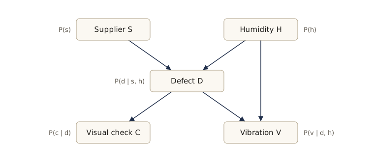
The network’s factorization is
\[P(s, h, d, v, c) = P(s)\,P(h)\,P(d \mid s, h)\,P(v \mid d, h)\,P(c \mid d).\]Every question about the network is answered from this joint. For a query variable \(X\) and observed evidence \(\mathbf{e}\), the posterior is
\[P(x \mid \mathbf{e}) = \frac{P(x, \mathbf{e})}{P(\mathbf{e})} = \alpha \sum_{\text{hidden}} P(x, \mathbf{e}, \text{hidden}),\]where we sum the joint over all variables that are neither queried nor observed, and \(\alpha\) is the constant that makes the result sum to one. This is inference by enumeration. With five binary variables the joint has only 32 entries, so we can build it as one array with einsum and answer questions by indexing and summing.
# variables in axis order s, h, d, v, c
# value 1 means: supplier b / high humidity / defective / high vibration / fail
P_S = np.array([0.7, 0.3])
P_H = np.array([0.6, 0.4])
P_D_SH = np.array([[[0.98, 0.02], [0.92, 0.08]],     # P(d | s, h), indexed [s, h, d]
                   [[0.90, 0.10], [0.75, 0.25]]])
P_V_DH = np.array([[[0.95, 0.05], [0.80, 0.20]],     # P(v | d, h), indexed [d, h, v]
                   [[0.15, 0.85], [0.10, 0.90]]])
P_C_D = np.array([[0.97, 0.03],                      # P(c | d), indexed [d, c]
                  [0.40, 0.60]])
joint_bn = np.einsum("s,h,shd,dhv,dc->shdvc", P_S, P_H, P_D_SH, P_V_DH, P_C_D)
AXES = "shdvc"

def query(target, evidence):
    """P(target | evidence) by enumeration; evidence is a dict like {'v': 1}."""
    idx = tuple(slice(evidence[a], evidence[a] + 1) if a in evidence else slice(None)
                for a in AXES)
    sub = joint_bn[idx]                        # keep only entries consistent with the evidence
    keep = AXES.index(target)
    p = sub.sum(axis=tuple(i for i in range(len(AXES)) if i != keep)).ravel()
    return p / p.sum()

print(f"joint sums to {joint_bn.sum():.6f};  numbers in the tables: "
      f"{1 + 1 + 4 + 4 + 2} versus {2**5 - 1} for a full joint table")
print(f"P(defective)                          = {query('d', {})[1]:.4f}")
print(f"P(defective | vibration high)         = {query('d', {'v': 1})[1]:.4f}")
print(f"P(defective | vibration high, humid)  = {query('d', {'v': 1, 'h': 1})[1]:.4f}")
print(f"P(defective | vibration high, fail)   = {query('d', {'v': 1, 'c': 1})[1]:.4f}")
print(f"P(supplier b)                         = {query('s', {})[1]:.4f}")
print(f"P(supplier b | visual check fails)    = {query('s', {'c': 1})[1]:.4f}")
joint sums to 1.000000;  numbers in the tables: 12 versus 31 for a full joint table
P(defective)                          = 0.0788
P(defective | vibration high)         = 0.4148
P(defective | vibration high, humid)  = 0.4042
P(defective | vibration high, fail)   = 0.9341
P(supplier b)                         = 0.3000
P(supplier b | visual check fails)    = 0.4853
The answers show three kinds of reasoning that come for free from the factorization. Evidence flows downward and upward: a high vibration reading raises the probability of a defect from under 8% to over 40%, and a failed visual check raises the probability that the material came from supplier b, even though the supplier is a cause and the check an effect. Evidence also combines: a failed visual check on top of the vibration makes a defect very likely. And evidence can explain away: learning that the shop was humid lowers the probability of a defect given high vibration slightly, from 0.415 to 0.404, even though humidity makes defects more likely. Humidity is also a second, innocent explanation for the vibration, and here the two effects nearly cancel; with a weaker link from humidity to defects the drop would be larger.
Enumeration is exponential in the number of variables, so for larger networks we exploit the factorization and push each sum as far inside the product as it will go. For the query \(P(d \mid v = \text{high})\),
\[P(d, v) = \sum_{s}\sum_{h} P(s)\,P(h)\,P(d \mid s, h)\,P(v \mid d, h)\sum_{c} P(c \mid d),\]and the innermost sum is 1, since it runs over one row of a conditional table. An unobserved node with no observed descendants drops out of the computation entirely. The cell checks this by hand.
# sum over s and h, with the C table left out entirely
P_dv = np.einsum("s,h,shd,dh->d", P_S, P_H, P_D_SH, P_V_DH[:, :, 1])
print(f"P(defective | vibration high), C summed out analytically: {P_dv[1] / P_dv.sum():.4f}")
print(f"sum over c of P(c | d) for each d: {P_C_D.sum(axis=1)}")
P(defective | vibration high), C summed out analytically: 0.4148
sum over c of P(c | d) for each d: [1. 1.]
Organizing such sums systematically gives variable elimination and, for tree-shaped graphs, message passing; networks with loops need more care. When we know nothing about the dependencies among features, the simplest assumption is that all features are conditionally independent given the class: a network with the class as the only parent of every feature. That is the naive Bayes model of the previous sections. Intro to ML, module 08 treats belief networks in full: conditional independence and d-separation, Markov random fields, and exact inference by message passing. Learning the tables from data is an estimation problem of the kind taken up in module 03.
Compound decision theory and context
Until now each pattern was classified on its own, as if the class of the next part had nothing to do with the class of the last. Often it does. Defects on a production line come in runs when a tool wears; letters in a word follow spelling; phonemes follow each other in speech. Using the dependence between neighboring states of nature is using context.
Suppose we observe \(n\) patterns \(\mathbf{X} = (\mathbf{x}_1, \dots, \mathbf{x}_n)\) and must decide the whole sequence of states \(\boldsymbol{\omega} = (\omega(1), \dots, \omega(n))\), where each \(\omega(i)\) is one of \(\omega_1, \dots, \omega_c\). If we can wait for all \(n\) observations before deciding, this is a compound decision problem; deciding each one as it arrives is the harder sequential version, which we do not treat. Bayes’ formula for the whole sequence is
\[P(\boldsymbol{\omega} \mid \mathbf{X}) = \frac{p(\mathbf{X} \mid \boldsymbol{\omega})\,P(\boldsymbol{\omega})}{\sum_{\boldsymbol{\omega}'} p(\mathbf{X} \mid \boldsymbol{\omega}')\,P(\boldsymbol{\omega}')},\]and with a zero–one loss on the whole sequence (any mistake anywhere costs 1), the Bayes rule picks the sequence with the largest posterior. Two simplifications make this workable. First, it is usually reasonable to assume that each observation depends only on its own state, so \(p(\mathbf{X} \mid \boldsymbol{\omega}) = \prod_i p(\mathbf{x}_i \mid \omega(i))\). Second, the prior \(P(\boldsymbol{\omega})\) carries the context, so we must not assume the states independent (that would throw the context away); a Markov chain, in which each state depends only on the previous one, is the usual compromise.
The difficulty is the sum over \(\boldsymbol{\omega}'\): there are \(c^n\) sequences. For a short sequence we can enumerate them. In the next cell, parts are good or defective in runs (a part has the same class as the previous one with probability 0.9), each part gives a reading from \(N(0, 1)\) or \(N(1.2, 1)\), and we decide sequences of 8 parts by enumerating all \(2^8 = 256\) possibilities. We compare three rules: classify each part on its own, ignoring context; pick the most probable sequence; and pick, at each position, the most probable state under the sequence posterior \(P(\omega(i) \mid \mathbf{X})\).
n_seq, stay = 8, 0.9
A_mc = np.array([[stay, 1 - stay], [1 - stay, stay]])      # P(omega(i) | omega(i-1))
pi0 = np.array([0.5, 0.5])                                 # also the stationary distribution
m_c, s_c = np.array([0.0, 1.2]), 1.0
seqs = np.array(list(product([0, 1], repeat=n_seq)))   # all 2^n sequences, shape (256, 8)
log_prior_seq = np.log(pi0[seqs[:, 0]]) + np.log(A_mc[seqs[:, :-1], seqs[:, 1:]]).sum(axis=1)

def simulate_runs(n_rep, gen):
    states = np.empty((n_rep, n_seq), dtype=int)
    states[:, 0] = gen.choice(2, size=n_rep, p=pi0)
    for i in range(1, n_seq):
        flip = gen.random(n_rep) >= stay
        states[:, i] = np.where(flip, 1 - states[:, i - 1], states[:, i - 1])
    return states, gen.normal(m_c[states], s_c)

def sequence_posterior(X):
    """P(omega | X) for every sequence omega (columns) and every observed row of X."""
    loglik = log_normal_1d(X[:, None, :], m_c[seqs][None, :, :], s_c).sum(axis=2)
    a = loglik + log_prior_seq
    return np.exp(a - logsumexp(a, axis=1, keepdims=True))

states, X_seq = simulate_runs(2000, np.random.default_rng(12))
post_seq = sequence_posterior(X_seq)
rules = {
    "each part alone (no context)": (X_seq > 0.6).astype(int),   # midpoint of the means
    "most probable sequence": seqs[post_seq.argmax(axis=1)],
    "most probable state per position": (post_seq @ seqs > 0.5).astype(int),
}
print("rule                               part errors   sequences with any error")
for name, dec in rules.items():
    part_err, seq_err = np.mean(dec != states), np.mean(np.any(dec != states, axis=1))
    print(f"{name:34s}  {part_err:.4f}        {seq_err:.4f}")
rule                               part errors   sequences with any error
each part alone (no context)        0.2811        0.9290
most probable sequence              0.1786        0.4895
most probable state per position    0.1691        0.5295
Context helps a great deal: both rules that use the Markov prior cut the part error rate from 0.28 to about 0.17–0.18, and the fraction of sequences with at least one error roughly in half. The comparison between them is a small lesson in loss functions. The most probable sequence is the Bayes rule for “any error in the sequence costs 1”, and it has the fewest sequences with an error. Choosing the most probable state at each position is the Bayes rule for “each wrong part costs 1”, and it has the fewest wrong parts. Neither is better in general; the loss decides.
Enumeration grows as \(c^n\) and is hopeless for long sequences. With a Markov prior, dynamic programming does the same work in time proportional to \(nc^2\): the Viterbi algorithm finds the most probable sequence, and the forward–backward algorithm gives the per-position posteriors. These are the hidden Markov model algorithms of module 03 (DHS §3.10), also derived in Intro to ML, module 13.
Summary
| Rule or model | What it needs | What it does |
|---|---|---|
| Bayes minimum-risk rule | priors, class-conditional densities, loss matrix | at each \(\mathbf{x}\), the action with smallest \(R(\alpha_i \mid \mathbf{x})\); minimizes overall risk |
| Minimum-error (MAP) rule | priors, densities; zero–one loss | largest posterior \(P(\omega_i \mid \mathbf{x})\); minimizes the error rate |
| Two-class Bayes rule | the same | likelihood-ratio test; costs and priors set only the threshold |
| Reject option | reject cost \(\lambda_r\) | reject when \(\max_i P(\omega_i \mid \mathbf{x}) < 1 - \lambda_r\) |
| Minimax | densities, losses; no priors | Bayes rule for the least favorable prior; risk independent of the prior |
| Neyman–Pearson | densities; a false-alarm limit \(\alpha\) | likelihood-ratio test with false-alarm rate \(\alpha\); most hits for that rate |
| Gaussian, \(\boldsymbol{\Sigma}_i = \sigma^2\mathbf{I}\) | means, \(\sigma^2\), priors | linear; boundary perpendicular to the line of means; nearest mean if priors are equal |
| Gaussian, \(\boldsymbol{\Sigma}_i = \boldsymbol{\Sigma}\) | means, shared \(\boldsymbol{\Sigma}\), priors | linear; nearest mean in Mahalanobis distance if priors are equal |
| Gaussian, arbitrary \(\boldsymbol{\Sigma}_i\) | means, covariances, priors | quadratic; boundaries are hyperquadrics, regions may be disconnected |
| Independent binary features | \(p_i\), \(q_i\), priors | linear in \(\mathbf{x}\), weights \(\ln[p_i(1-q_i)/(q_i(1-p_i))]\) |
| Missing or noisy features | the full model, a noise model | marginalize the unobserved values (weighted by the noise model) |
| Belief network | a graph and conditional tables | posteriors by summing the factored joint over hidden variables |
| Compound decision | a prior over sequences | most probable sequence, or most probable state per position |
Ideas to carry forward:
- The Bayes rule is found pointwise: at each \(\mathbf{x}\), take the action with the smallest conditional risk. Every criterion in this module, minimum error, minimum risk, reject, Neyman–Pearson, and the compound rules, is this one idea with a different loss or constraint.
- For two classes every sensible criterion leads to a likelihood-ratio test. Costs, priors, and constraints only move the threshold, which moves the operating point along the ROC curve.
- The Bayes error is the floor for any classifier using the same features. It can be computed by integration or Monte Carlo in low dimensions and bounded in closed form (Chernoff, Bhattacharyya) for Gaussians in any dimension.
- Everything here assumed the densities known. From module 03 on, we estimate them from samples, or skip them and train discriminant functions directly; the rules of this module are the target those methods aim at.
Exercises
- Show that with \(c\) classes, zero–one loss, and a reject action of cost \(\lambda_r\), the Bayes rule rejects exactly when \(\max_i P(\omega_i \mid \mathbf{x}) < 1 - \lambda_r\), and that it never rejects if \(\lambda_r \ge (c-1)/c\). Then extend the reject cell to plot error rate against reject rate as \(\lambda_r\) runs from 0 to 0.5 for the inspection problem, and explain why the curve is convex.
- Prove that the Bayes risk \(R^{*}(P)\) is a concave function of the prior \(P = P(\omega_1)\) in a two-class problem. Then compute the minimax rule for the inspection problem under the shipping loss (\(\lambda_{12} = 8\), \(\lambda_{21} = 1\)) with
lr_testandbisect, and report the least favorable prior and the minimax risk. - For two univariate normal classes with equal variance \(\sigma^2\) and means \(\mu_1 < \mu_2\), derive the Neyman–Pearson threshold and hit rate for a false-alarm limit \(\alpha\) in terms of \(\Phi^{-1}\) and \(d'\). Check your formula against a numerical solution for \(d' = 1.3\) and \(\alpha = 0.01\).
- In case 1 of the Gaussian discriminants, show that the boundary between two classes lies beyond the mean of the less probable class when \(\ln[P(\omega_i)/P(\omega_j)] > \lVert \boldsymbol{\mu}_i - \boldsymbol{\mu}_j \rVert^2/(2\sigma^2)\). Find a prior for the case 1 example of the notes where this happens and verify it with
classify. - For two Gaussian classes with a shared covariance, let \(\Delta^2 = (\boldsymbol{\mu}_1 - \boldsymbol{\mu}_2)^{t}\boldsymbol{\Sigma}^{-1}(\boldsymbol{\mu}_1 - \boldsymbol{\mu}_2)\). Show that the linear discriminant \(g(\mathbf{x})\) is normal under each class with variance \(\Delta^2\) and means \(\pm\Delta^2/2 + \ln[P(\omega_1)/P(\omega_2)]\), and derive a closed form for the Bayes error in terms of \(\Phi\). Check it against the grid values for cases 1 and 2 in the notes.
- Show that \(\ln \int p^{\beta}(\mathbf{x} \mid \omega_1)\,p^{1-\beta}(\mathbf{x} \mid \omega_2)\,d\mathbf{x}\) is convex in \(\beta\) (differentiate twice and recognize a variance). For two Gaussians with a shared covariance, show that \(k(\beta) = \beta(1-\beta)\Delta^2/2\) and find \(\beta^{*}\) in closed form for arbitrary priors. Compare with
golden_minfor the inspection problem made equal-variance. - For the equal-variance signal detection model, show that the slope of the ROC curve at the point produced by threshold \(x^{*}\) equals the likelihood ratio \(p(x^{*} \mid \omega_2)/p(x^{*} \mid \omega_1)\), and that the area under the curve is \(\Phi(d'/\sqrt{2})\). Then repeat the simulated experiment 500 times with different seeds and report the mean and spread of the estimated \(d'\); how does the spread change with the threshold?
- Let the binary features of the checks example be dependent: under each class, checks 1 and 2 are both flagged with an extra probability, so that \(P(x_1 = 1, x_2 = 1 \mid \omega_j)\) exceeds \(P(x_1 = 1 \mid \omega_j)P(x_2 = 1 \mid \omega_j)\). Build such a model (choose your own joint table for \((x_1, x_2)\)), compute its exact Bayes error by enumerating the 16 corners, and compare it with the error of the naive Bayes rule that assumes independence.
- In the missing-feature example, suppose instead that \(x_2\) is missing and \(x_1\) observed. Compute the marginal posterior for \(x_1 = 1.5\), compare with mean imputation, and measure both error rates on the test set. Why is the gap between the two strategies smaller here?
- In the belief network, compute \(P(h = \text{high} \mid v = \text{high})\) and \(P(h = \text{high} \mid v = \text{high}, c = \text{fail})\) and explain the change in words. Then write a function that computes \(P(d \mid \mathbf{e})\) by pushing sums inside the product for any evidence on \(\{s, h, v, c\}\), and check it against
queryfor all 81 combinations of observed and unobserved values. - Implement the Viterbi algorithm for the compound decision example (work in log space) and check that it returns the same sequence as brute-force enumeration on all 2000 simulated sequences. Then run it on sequences of length 200, where enumeration is impossible, and report the part error rate.
- In your own words: why does the Bayes rule, which is optimal, still make errors, and what would have to change about the features or the problem for its error to go down?
Going further
- R. O. Duda, P. E. Hart, and D. G. Stork, Pattern Classification, 2nd ed., chapter 2 — the source for this module. Problems 3–7 (minimax and Neyman–Pearson), 13–14 (the reject option), 23–30 (normal densities and their discriminants), 31–42 (error integrals, Chernoff and Bhattacharyya bounds, signal detection), 43–47 (discrete features), 48–49 (missing and noisy features), 50–51 (belief networks), and 52 (compound decisions) pair well with the sections above, as do computer exercises 1–9.
- J. Neyman and E. S. Pearson, “On the problem of the most efficient tests of statistical hypotheses”, Philosophical Transactions of the Royal Society A, 1933 — the lemma behind the Neyman–Pearson criterion.
- C. K. Chow, “On optimum recognition error and reject tradeoff”, IEEE Transactions on Information Theory, 1970 — the error–reject tradeoff of the reject option, in depth.
- D. M. Green and J. A. Swets, Signal Detection Theory and Psychophysics (Wiley, 1966) — the classic account of d′ and ROC analysis.
- The machine-learning notes cover the same foundations from Bishop’s angle: decision theory and the reject option in Intro to ML, module 01, Gaussian identities in module 02, generative classifiers and naive Bayes in module 04, and belief networks with exact inference in module 08.
These notes follow the chapters of R. O. Duda, P. E. Hart, and D. G. Stork, Pattern Classification, 2nd edition (Wiley, 2001), the course text. The explanations, code, figures, and exercises here are written for this course; the book remains the reference, with the full derivations, worked examples, and many more problems.