CSE 455/555 · Module 01 · Session 1
Introduction: Machine Perception and the Design Cycle
What a pattern recognition system is made of — sensing, segmentation, features, classification, postprocessing — and the design cycle from data collection to evaluation.
Companion reading: Duda, Hart & Stork, Pattern Classification, chapter 1, “Introduction”
By the end of this module you can
- Describe the stages of a pattern recognition system — sensing, segmentation and grouping, feature extraction, classification, postprocessing — and name a problem that each stage has to solve.
- Fit a one-feature threshold classifier by searching over thresholds, and explain why its training error is an optimistic estimate of its error on new data.
- Move a decision threshold to account for unequal costs of the two kinds of mistake, and compute an average cost from a loss matrix.
- Derive the linear decision boundary of the nearest-mean classifier, \(g(\mathbf{x}) = \mathbf{w}^{t}\mathbf{x} + w_0\), and use it with two standardized features.
- Show with an experiment that a rule flexible enough to classify every training sample correctly (1-nearest-neighbor) can generalize worse than a straight line.
- Walk through the design cycle — data collection, feature choice, model choice, training, evaluation — and explain why computational complexity at decision time matters.
- Distinguish supervised learning, unsupervised learning (clustering), and learning with a critic, and run a two-cluster k-means on unlabeled data.
Contents
- Machine perception
- An example: sorting lemons from limes
- Pattern recognition systems
- The design cycle
- Learning and adaptation
- Conclusion and a map of the course
- Summary
- Exercises
- Going further
Look at a lemon and a lime side by side and you know at once which is which. You did not measure anything, consult a rule, or compute a probability; the decision just arrived. Pattern recognition is the study of how to make machines do the same thing: take in raw measurements of some object or event and act on the category it belongs to. This course is about the ideas and algorithms that make that possible, from the optimal decision rule when everything about the problem is known, to rules learned from examples, to groupings found in data with no labels at all.
The course follows R. O. Duda, P. E. Hart, and D. G. Stork, Pattern Classification, 2nd edition (Wiley, 2001), which we call DHS. There is one module per chapter: this module goes with chapter 1, module 02 with chapter 2, and so on. The notes are our own rewrite, with our own examples and NumPy code; each module points to the book sections that hold the full derivations and many more problems. The code cells run top to bottom in one Python session, and the output under each cell is the real output of that run.
Chapter 1 of DHS asks many questions and answers few of them on purpose: it lays out the problems the rest of the book solves. We do the same, but we make each question concrete with a small running example you can run in a few seconds. A packing line has to sort lemons from limes using two measurements of each fruit. Along the way we will see a single-feature threshold, the gap between training and held-out error, costs that are not symmetric, a linear boundary in two dimensions, and a rule that fits its training data perfectly and still does worse on new fruit. Everything here is informal; later modules make each piece precise.
Machine perception
People recognize faces, voices, handwriting, and ripe fruit without effort, but the processes behind that ease are far from simple. Building machines that do the same is useful in its own right — speech recognition, fingerprint matching, reading handwritten addresses, identifying DNA sequences, inspecting parts on a production line, flagging fraudulent transactions — and the attempt also teaches us how hard the problems solved by natural perception are. Some designs even borrow from biology, in their algorithms or in the special-purpose hardware they run on.
Across all these applications the task has the same shape. A pattern is the description of one object or event: an image, a sound clip, a vector of measurements. The object belongs to one of \(c\) categories (or classes), which we write \(\omega_1, \dots, \omega_c\). A classifier is a rule that takes a pattern and returns a category, or better, a degree of belief in each category from which a decision can be made. Most of this course is about how to design classifiers and how to judge them.
An example: sorting lemons from limes
Suppose a produce packer wants to automate the sorting of a mixed stream of lemons and limes on a conveyor belt. A camera looks down at the belt; from each image we can measure things about each fruit: its size, its color, the texture of its skin, its shape. These candidate measurements are features. Sensor noise, uneven lighting, and natural variety all make the measured values spread out within each kind of fruit.
The general approach, which the rest of the course develops in many forms, is to posit a model for each category — a description, usually mathematical, of what patterns from that category look like — and then to assign each new pattern to the category whose model explains it best. Here a model could be as simple as “limes are shorter than lemons” or as detailed as a probability density over all measured features.
The data
We do not have a packing line, so we simulate one. Each fruit is described by two features: \(x_1\), its length in millimeters along the long axis, and \(x_2\), its hue angle in degrees (on the color wheel 60 is yellow and 120 is green, so limes sit higher). The category is \(\omega_1\) = lemon or \(\omega_2\) = lime. In code the labels are the integers 0 (lemon) and 1 (lime), and a data set is a matrix X of shape (n, d) with one row per fruit.
We draw each class from a two-dimensional Gaussian whose means and spreads we pick: lemons are longer and yellower on average, limes shorter and greener, and the two overlap. We make a training set of 60 fruit per class, which we use to design the classifier, and a separate held-out set (or test set) of 400 per class, which we use only to measure how well the finished classifier does on fruit it has not seen.
import numpy as np

np.set_printoptions(precision=4, suppress=True)
rng = np.random.default_rng(455)

# Class 0 = lemon (omega_1), class 1 = lime (omega_2). Features: length (mm), hue angle (degrees).
MEANS = np.array([[71.0, 64.0],     # lemon
                  [60.0, 74.0]])    # lime
SDS = np.array([[6.0, 6.0],
                [5.0, 6.0]])
RHO = 0.2                           # within-class correlation of length and hue

def make_citrus(n_per_class, rng):
    """n_per_class lemons, then n_per_class limes: X of shape (2n, 2) and labels y in {0, 1}."""
    X, y = [], []
    for j in range(2):
        z = rng.standard_normal((n_per_class, 2))
        z[:, 1] = RHO * z[:, 0] + np.sqrt(1 - RHO**2) * z[:, 1]   # correlate the two features
        X.append(MEANS[j] + SDS[j] * z)
        y.append(np.full(n_per_class, j))
    return np.vstack(X), np.concatenate(y)

X_tr, y_tr = make_citrus(60, rng)     # training set: 120 fruit
X_te, y_te = make_citrus(400, rng)    # held-out set: 800 fruit
for j, name in enumerate(["lemon", "lime"]):
    m = X_tr[y_tr == j].mean(axis=0)
    print(f"{name}: n = {np.sum(y_tr == j)}, mean length {m[0]:.1f} mm, mean hue {m[1]:.1f} deg")
lemon: n = 60, mean length 69.9 mm, mean hue 63.6 deg
lime: n = 60, mean length 59.6 mm, mean hue 74.0 deg
One feature and a threshold
Someone on the packing floor tells us that lemons are usually longer than limes. That suggests the simplest possible classifier: measure the length \(x_1\) and call the fruit a lime if \(x_1 < \theta\), a lemon otherwise. The number \(\theta\) is a threshold, and the point \(x_1 = \theta\) is the decision boundary of this one-dimensional rule.
How should we pick \(\theta\)? With a training set in hand, the obvious answer is to try every candidate and keep the one that makes the fewest mistakes on the training fruit. Only the ordering of the training values matters, so it is enough to try the midpoints between consecutive sorted values. The fraction of samples a rule gets wrong is its error rate. We write the search once, for either feature and either direction, because we will reuse it. The function also takes a loss matrix lam, where lam[i, j] is the cost of deciding class \(i\) when the truth is class \(j\); with zeros on the diagonal and ones off it, the average cost is the error rate.
LAM_01 = np.array([[0.0, 1.0],
                   [1.0, 0.0]])       # zero-one loss: lam[i, j] = cost of deciding i when the truth is j

def threshold_rule(x, theta, sign):
    """Decide lime (1) when sign * (x - theta) > 0, lemon (0) otherwise."""
    return (sign * (x - theta) > 0).astype(int)

def mean_cost(pred, y, lam=LAM_01):
    """Average cost per sample; with the zero-one loss this is the error rate."""
    return lam[pred, y].mean()

def fit_threshold(x, y, sign, lam=LAM_01):
    """Try every midpoint between sorted training values and keep the cheapest (first one on ties)."""
    xs = np.sort(x)
    cands = (xs[:-1] + xs[1:]) / 2
    costs = np.array([mean_cost(threshold_rule(x, c, sign), y, lam) for c in cands])
    k = int(np.argmin(costs))
    return cands[k], costs[k]

theta_len, _ = fit_threshold(X_tr[:, 0], y_tr, -1)
for f, sign, name in [(0, -1, "length"), (1, +1, "hue")]:
    theta, err_tr = fit_threshold(X_tr[:, f], y_tr, sign)
    err_te = mean_cost(threshold_rule(X_te[:, f], theta, sign), y_te)
    print(f"{name:6s}: theta = {theta:6.2f}   training error {err_tr:.3f}   held-out error {err_te:.3f}")
length: theta =  63.95   training error 0.142   held-out error 0.181
hue   : theta =  67.98   training error 0.158   held-out error 0.204
Length alone gets about one training fruit in seven wrong, and hue does slightly worse. Both rules show something we must keep in mind all course long: each threshold was chosen to do well on the training fruit, so its training error flatters it. On the held-out fruit both error rates rise by roughly four percentage points.
Training error and held-out error
The goal of a classifier is to act correctly on patterns it has never seen, a property called generalization. The error rate on the training set is a poor guide to it because the training set was used to choose the rule: whatever quirks those particular 120 fruit happen to have, the search for \(\theta\) has partly adapted to them. The error on a held-out set that played no part in the design is an honest estimate, at the price of setting data aside.
Watch out. Every choice made while looking at a data set — the threshold, the features, the kind of classifier, even how the features were scaled — is part of training. An error rate measured on data that influenced any of those choices is optimistic. Keep the held-out set out of the design until the end, and use it once.
When one mistake costs more than the other
So far both kinds of mistake count the same. That is often not true. Suppose the lemons go to a juice bar and the limes are bagged for sale. A lime that ends up with the lemons is squeezed along with them and nobody minds much; a lemon found in a bag of limes brings a complaint and a refund. Say the second mistake costs four times as much as the first. In the loss-matrix notation, deciding lime (\(\omega_2\)) when the fruit is a lemon (\(\omega_1\)) costs \(\lambda_{21} = 4\), and the opposite mistake costs \(\lambda_{12} = 1\).
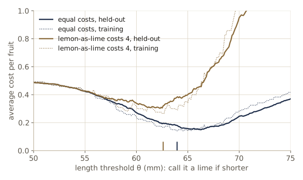
Now the goal is not the fewest errors but the smallest average cost. Because calling a fruit a lime has become the riskier decision, we should demand stronger evidence before making it: the threshold on length should move down, so that only clearly short fruit are called limes. We let the training data find the new threshold.
LAM_COST = np.array([[0.0, 1.0],
                     [4.0, 0.0]])     # a lemon sent to the lime bags (decide 1, truth 0) costs 4

for label, lam in [("equal costs", LAM_01), ("lemon-as-lime costs 4", LAM_COST)]:
    theta, _ = fit_threshold(X_tr[:, 0], y_tr, -1, lam)
    pred_te = threshold_rule(X_te[:, 0], theta, -1)
    lemons_as_limes = np.mean(pred_te[y_te == 0] == 1)
    limes_as_lemons = np.mean(pred_te[y_te == 1] == 0)
    print(f"{label:22s} theta = {theta:.2f}   lemons called lime {lemons_as_limes:.3f}   "
          f"limes called lemon {limes_as_lemons:.3f}")
    print(f"{'':22s} held-out cost under the 4:1 losses: {mean_cost(pred_te, y_te, LAM_COST):.3f}")
equal costs            theta = 63.95   lemons called lime 0.138   limes called lemon 0.225
                       held-out cost under the 4:1 losses: 0.388
lemon-as-lime costs 4  theta = 62.60   lemons called lime 0.083   limes called lemon 0.310
                       held-out cost under the 4:1 losses: 0.320
The threshold drops, far fewer lemons land in the lime bags, more limes land with the lemons, and the average cost under the 4:1 losses falls even though the total number of errors goes up. The figure below traces the held-out average cost as a function of the threshold for both loss matrices.
Choosing a decision rule to minimize an expected cost is the subject of decision theory, and it is where module 02 begins: there the average cost becomes the risk, the threshold becomes a comparison of posterior probabilities weighted by the losses, and we will be able to say exactly where the best threshold lies when the class densities are known.
A second feature
Even the best length threshold leaves many errors, and no single feature we have does much better. The next step is to use both features at once. Each fruit is now a point, the feature vector
\[\mathbf{x} = \begin{pmatrix} x_1 \\ x_2 \end{pmatrix},\]in a two-dimensional feature space, and a classifier divides that plane into two decision regions, one per class, separated by a decision boundary.
The two features are in different units, millimeters and degrees, so before comparing distances we standardize them: subtract the training mean of each feature and divide by its training standard deviation. This is a small but real design decision, a piece of preprocessing, and it uses training statistics only.
A simple rule in the standardized space is the nearest-mean classifier: compute the mean \(\mathbf{m}_1\) of the training lemons and \(\mathbf{m}_2\) of the training limes, and assign a new fruit to the class whose mean is closer. Its boundary is a straight line. To see why, write out “closer to \(\mathbf{m}_2\)” and expand the squared distances; the quadratic term \(\mathbf{x}^{t}\mathbf{x}\) appears on both sides and cancels:
\[\begin{aligned} \lVert \mathbf{x} - \mathbf{m}_2 \rVert^2 < \lVert \mathbf{x} - \mathbf{m}_1 \rVert^2 &\iff -2\mathbf{m}_2^{t}\mathbf{x} + \mathbf{m}_2^{t}\mathbf{m}_2 < -2\mathbf{m}_1^{t}\mathbf{x} + \mathbf{m}_1^{t}\mathbf{m}_1 \\ &\iff (\mathbf{m}_2 - \mathbf{m}_1)^{t}\mathbf{x} - \tfrac{1}{2}\left(\mathbf{m}_2^{t}\mathbf{m}_2 - \mathbf{m}_1^{t}\mathbf{m}_1\right) > 0 . \end{aligned}\]So the rule is “decide \(\omega_2\) when \(g(\mathbf{x}) > 0\)” for the linear discriminant function
\[g(\mathbf{x}) = \mathbf{w}^{t}\mathbf{x} + w_0, \qquad \mathbf{w} = \mathbf{m}_2 - \mathbf{m}_1, \qquad w_0 = -\tfrac{1}{2}\left(\lVert \mathbf{m}_2 \rVert^2 - \lVert \mathbf{m}_1 \rVert^2\right).\]The boundary \(g(\mathbf{x}) = 0\) is the perpendicular bisector of the segment joining the two means. The superscript \(t\) is the transpose, as in DHS; the Intro to ML notes, which follow Bishop, write \(\mathbf{w}^{\mathrm{T}}\) and name classes \(\mathcal{C}_k\) instead of \(\omega_j\).
mu_hat, sd_hat = X_tr.mean(axis=0), X_tr.std(axis=0)

def standardize(X):
    return (X - mu_hat) / sd_hat           # training statistics only

def fit_nearest_mean(Z, y):
    m1, m2 = Z[y == 0].mean(axis=0), Z[y == 1].mean(axis=0)
    w = m2 - m1                            # w = m2 - m1
    w0 = -0.5 * (m2 @ m2 - m1 @ m1)        # w0 = -(||m2||^2 - ||m1||^2) / 2
    return w, w0

def linear_rule(Z, w, w0):
    return (Z @ w + w0 > 0).astype(int)    # decide lime when g(x) > 0

Z_tr, Z_te = standardize(X_tr), standardize(X_te)
w, w0 = fit_nearest_mean(Z_tr, y_tr)
print("w =", w, f"  w0 = {w0:.1e}")
print(f"training error {mean_cost(linear_rule(Z_tr, w, w0), y_tr):.3f}   "
      f"held-out error {mean_cost(linear_rule(Z_te, w, w0), y_te):.3f}")

# check: the linear rule agrees with comparing the two distances directly
m1, m2 = Z_tr[y_tr == 0].mean(axis=0), Z_tr[y_tr == 1].mean(axis=0)
direct = (np.sum((Z_te - m2)**2, axis=1) < np.sum((Z_te - m1)**2, axis=1)).astype(int)
print("agrees with the distance comparison on all held-out fruit:",
      bool(np.all(direct == linear_rule(Z_te, w, w0))))
w = [-1.4195  1.3684]   w0 = -3.6e-15
training error 0.058   held-out error 0.066
agrees with the distance comparison on all held-out fruit: True
Two features cut the held-out error to about a third of the best single feature’s. In the scatter plot the reason is visible: along either axis alone the classes overlap heavily, but the clouds are much better separated along a diagonal direction that uses both measurements. (The bias \(w_0\) is zero up to rounding because the two classes are equally large: after standardizing, their means sit on opposite sides of the origin, so the bisector passes through it.)
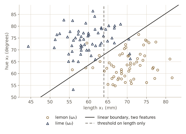
It is tempting to conclude that more features are always better. They are not free: each must be measured, some are redundant (a feature that is a near copy of another adds little), and with a fixed amount of training data, adding dimensions can make a classifier worse. That last effect, the curse of dimensionality, is taken up in module 03.
A boundary that is too flexible
The straight line still misclassifies a few training fruit. We could insist on a rule that gets every training fruit right. The 1-nearest-neighbor rule does exactly that: give a new fruit the label of the single closest training fruit. Every training point is its own nearest neighbor, so the training error is zero, and the boundary can bend around every stray point.
def nn1_rule(Zq, Z, y):
    """Label of the closest training point (1-nearest-neighbor)."""
    d2 = np.sum((Zq[:, None, :] - Z[None, :, :])**2, axis=2)   # (n_query, n_train) squared distances
    return y[np.argmin(d2, axis=1)]

print(f"1-NN:   training error {mean_cost(nn1_rule(Z_tr, Z_tr, y_tr), y_tr):.3f}   "
      f"held-out error {mean_cost(nn1_rule(Z_te, Z_tr, y_tr), y_te):.3f}")
print(f"linear: training error {mean_cost(linear_rule(Z_tr, w, w0), y_tr):.3f}   "
      f"held-out error {mean_cost(linear_rule(Z_te, w, w0), y_te):.3f}")
1-NN:   training error 0.000   held-out error 0.125
linear: training error 0.058   held-out error 0.066
Perfect on the training data, worse on new fruit. The 1-NN boundary has tuned itself to the accidents of this particular sample — a lime that happened to be long, a lemon that happened to be green — rather than to the underlying difference between lemons and limes. This is overfitting, and the figure makes it visible.
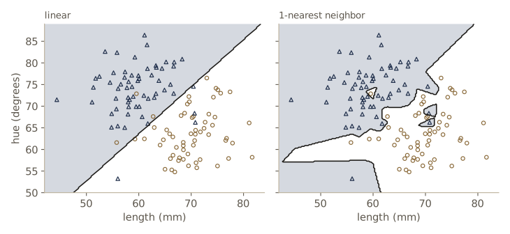
The preference for the simpler rule is a version of an old principle, usually credited to William of Occam: do not multiply entities beyond necessity. In pattern recognition the point is practical. A boundary as complicated as the 1-NN one needs far more data to be trusted, and even then a moderately smooth boundary, somewhere between the straight line and the jagged one, usually does best on new patterns. How to find that middle ground in a principled way — how to measure complexity, trade it against fit, and predict the error on new data — is one of the central questions of the course. The same phenomenon with polynomials of increasing degree is worked through in Intro to ML, module 01; nearest-neighbor rules get a full treatment, including why they are much better than this example suggests when data are plentiful, in module 04.
Note. Nothing about lemons and limes told us which classifier to use. The same features could serve a different task — separating ripe from unripe fruit, or damaged from sound — and that task would call for different decisions, different costs, and perhaps different features. Decisions are always relative to a task and its costs, which is one reason a single general-purpose recognizer is so hard to build.
Models, representations, and domain knowledge
Different kinds of model lead to different branches of the field. In statistical pattern recognition, which takes most of this course, each category is described by the probability distribution of its features, and noise is part of the model. Neural networks are sometimes treated as a separate discipline, but for our purposes they are a close relative of the statistical approach, as module 06 will show. When a category is better described by crisp rules than by a distribution — whether a string of symbols is a well-formed expression, say — we are in syntactic pattern recognition, with rules and grammars as models (module 08).
Behind every successful classifier is a good representation: a way of describing patterns so that ones calling for the same action are near each other and ones calling for different actions are far apart. Patterns may be vectors of real numbers, lists of attributes, strings, or descriptions of parts and their relations. Fewer features usually mean simpler regions and easier training; features that are robust, insensitive to noise, matter as much as features that separate the classes; and a deployed system may need to decide quickly with little memory.
When training data are scarce, knowledge of the domain matters more. An extreme form of this is analysis by synthesis: if we have a model of how patterns are produced, we classify a pattern by working out how it was generated. A speech recognizer built this way would ask which movements of the jaw, lips, and tongue could have produced a sound, since those movements are what the many acoustically different versions of the same syllable share. Recovering the generating process from the observed pattern is usually very hard, but milder versions are common: a handwriting recognizer may first recover the pen strokes and then read the character from them. Some categories are unified mainly by function: chairs come in endless shapes, and what they share is that a person can sit on them, which is a property we can only reach by reasoning about the object, well beyond pattern classification in the narrow sense.
Related fields
Pattern classification overlaps several neighboring fields, and the differences are instructive.
- Hypothesis testing in statistics decides whether the data are consistent with a null hypothesis, rejecting it when the data would be unlikely under it. It could tell us whether a batch of fruit contains one kind or two; classification has to say which kind each fruit is.
- Image processing turns an image into another image — rotating it, sharpening it, correcting its contrast — usually keeping all the information. Feature extraction deliberately throws information away.
- An associative memory takes a pattern and returns a stored, representative pattern. It reduces information somewhat; classification reduces it much further, down to a category label. A camera frame of thousands of pixels becomes a single bit, lemon or lime, and there is no way back from the label to the image.
- Regression finds a function that predicts a continuous output from inputs (for example, a fruit’s weight from its length). Interpolation fills in a function between points where it is known. Density estimation estimates the probability density of the features within a category. All three are used inside pattern recognition, density estimation above all: estimate the density of each class, then classify by comparing them. Modules 03 and 04 do exactly that.
Pattern recognition systems
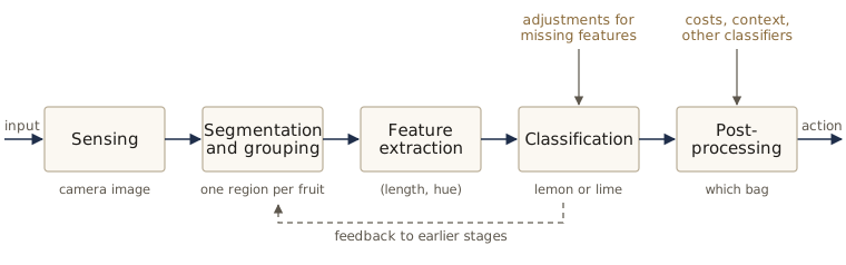
A working system is more than a classifier. The figure shows the usual stages, with our packing line as the running illustration beneath each one.
Sensing
The input comes from a transducer — a camera, a microphone, an accelerometer, a spectrometer. Its bandwidth, resolution, sensitivity, distortion, noise, and delay set limits that no later stage can undo. A camera that cannot tell yellow-green from green under the packing-house lights makes hue useless as a feature. Sensor design is its own discipline and outside this course, but it shapes everything downstream.
Segmentation and grouping
Our example quietly assumed that each fruit arrives alone. On a real belt fruit touch and overlap, and the system must decide where one ends and the next begins: this is segmentation. It is a chicken-and-egg problem: it would be easier to segment the image if we already knew what the objects were, and easier to recognize them if they were already segmented. Two touching limes look like one long fruit, and a length measured on that blob would call it a lemon. Segmentation ranks among the hardest problems in the field. In speech it is worse still, because neighboring sounds influence each other: the way a speaker shapes a vowel often starts to color the consonants before it, so there is no clean cut between them.
The companion problem is grouping: deciding which pieces belong together as one object. A lemon with its leaf still attached produces two regions in the image that should be treated as one fruit; the dot and stem of the letter i are two marks read as one symbol. A reader seeing the word THEREIN does not stop to consider THE, HERE, or REIN, even though each is a legitimate word inside it. Good recognizers seem to absorb as much of the input into one category as makes sense, and no more; doing that automatically is hard.
Feature extraction
The line between feature extraction and classification is somewhat arbitrary. A perfect feature extractor would make classification trivial (imagine a feature that simply equals the class), and an all-powerful classifier would need no feature extraction at all. We separate the two for practical reasons: feature extraction depends heavily on the domain, while classification can be studied in general.
The aim is features whose values are similar within a category and different between categories, and in particular features that are invariant to transformations of the input that do not change the category. A fruit’s position on the belt should not matter, so its features should be invariant to translation. The fruit may lie at any angle, so we measure length along its own long axis to make the feature invariant to rotation. Lighting drifts during the day, so hue should be measured against a reference white. But we do not want invariance to scale: size is one of our features, and limes are smaller. Which invariances are wanted depends on the task.
Other domains bring harder transformations. Rotating an object in three dimensions hides some parts (occlusion) and reveals others; moving it toward the camera changes its image by projective distortion. Speech varies in loudness, in timing, and in rate, and faster speech does not compress every sound uniformly. Handwriting varies with pen width and writing speed, and a hand changes shape as it grasps something (nonrigid deformation). The methods of this course cannot replace domain knowledge here, but they can make features less sensitive to noise and help choose a good subset from many candidates (feature selection, see module 03).
Classification
The classifier uses the feature vector to assign the object to a category or, more usefully, to report how probable each category is. Because feature vectors abstract away the domain, a largely domain-independent theory of classification is possible, and most of this course is about it.
How hard classification is depends on the spread of feature values within each category compared with the distance between categories. Part of the within-class spread is noise, which we define broadly as any property of the sensed pattern due to randomness in the world or the sensor rather than to the underlying model. Every interesting problem has some. What is the best classifier in the presence of noise, and what is the best error rate any classifier could achieve? Module 02 answers both when the distributions are known.
Another practical issue is missing features. If glare hides a fruit’s color, the camera returns no hue. Our two-feature rule was designed assuming both features, so what should it do? Two tempting fixes are to treat the missing hue as zero, or to plug in the average hue and carry on. The next cell tries both and compares them with the threshold we designed for length alone.
def plug_in_hue(X, hue_value):
    Xm = X.copy()
    Xm[:, 1] = hue_value       # pretend every fruit has this hue
    return standardize(Xm)

err_zero = mean_cost(linear_rule(plug_in_hue(X_te, 0.0), w, w0), y_te)
err_mean = mean_cost(linear_rule(plug_in_hue(X_te, mu_hat[1]), w, w0), y_te)
err_len_only = mean_cost(threshold_rule(X_te[:, 0], theta_len, -1), y_te)
print(f"hue plugged in as 0 degrees:   held-out error {err_zero:.3f}")
print(f"hue plugged in as its mean:    held-out error {err_mean:.3f}")
print(f"length-only threshold rule:    held-out error {err_len_only:.3f}")
# with z2 = 0 the rule g > 0 becomes z1 < -w0 / w1: a threshold on length
print(f"length threshold implied by the mean plug-in: {mu_hat[0] + sd_hat[0] * (-w0 / w[0]):.2f} mm")
hue plugged in as 0 degrees:   held-out error 0.500
hue plugged in as its mean:    held-out error 0.158
length-only threshold rule:    held-out error 0.181
length threshold implied by the mean plug-in: 64.77 mm
Treating the missing hue as zero degrees (a deep red, far from any real fruit) sends every fruit to the lemon side, which is no better than guessing. Plugging in the mean does reasonably well here, even a little better than our length threshold, which was a slightly unlucky choice from 120 fruit. But look at why: with the hue fixed, the rule becomes a threshold at the training mean length, and that happens to sit near the middle of the two classes only because our classes are equally common and similarly spread. Nothing in the method looked at how the classes are distributed along length; with unequal class sizes or unequal costs the plugged-in threshold would generally land in the wrong place. The better approach is to base the decision on the features that are present, averaging over what the missing one might have been; DHS §2.10 and module 02 show how.
Postprocessing
A classifier’s output is used to choose an action — send this fruit to the juice bar, bag that one — and each action has consequences. The postprocessor turns the classifier’s output into a recommended action. The simplest measure of performance is the error rate on new patterns, and minimizing it is common. When mistakes have different costs, as they did above, we want instead to minimize the expected cost, which is called the risk. Can we estimate the risk before deploying the system? Can we know the smallest risk any classifier could achieve, and so tell whether ours is close or the problem is simply hard?
The postprocessor can also use context, information beyond the pattern itself. If the crate being unloaded came from a lime grower, a borderline fruit is probably a lime. In reading text, a smudged character between T and E in “T?E” is almost certainly H. Context can be subtle: a mumbled phrase that means nothing in isolation is clear when you know where and when it was said.
Finally, we can combine multiple classifiers, each looking at a different aspect of the input — for fruit, one using the camera and one using a near-infrared sensor; for speech, one using the sound and one watching the lips. When they agree there is nothing to decide; when they disagree, how much weight should each get? A lone dissenter might be the only one that knows about a rare case, or it might just be wrong. Module 09 studies ways to pool classifiers.
In practice. The methods in this course mainly design the classification stage. They help with segmentation, feature extraction, and postprocessing too, where those problems are not tied to one domain. But good performance on hard real problems almost always comes from combining general methods with specific knowledge of the domain.
The design cycle
Building a pattern recognition system is iterative. We collect data, choose features, choose a model, train, and evaluate, and the evaluation usually sends us back to an earlier step. Prior knowledge about the domain — such as the invariances just discussed — feeds into the choice of features and of model. Our lemon–lime example already went around this loop several times: one feature was not good enough, so we added a second; a straight line left errors, so we tried a more flexible rule; the evaluation said that was worse.
Data collection
Collecting and labeling data is often a surprisingly large share of a project’s cost. A small set of typical examples may be enough to see whether an idea is feasible, but a deployed system needs much more. How much is enough, and how do we know the data are representative of what the system will meet? Our simulated data are representative by construction; real data are not. Fruit from a different grower, a different season, or a different camera may differ from the training set in ways that no amount of training data from the old source can reveal.
Data also limit how precisely we can evaluate. An error rate measured on \(n\) held-out samples is itself an estimate with sampling noise; treating each held-out fruit as an independent trial with error probability \(p\), its standard error is \(\sqrt{p(1-p)/n}\).
Feature choice
Choosing features depends on the domain. Example data help, but prior knowledge often matters more: the packer’s remark that lemons are longer, or the fact that ripe limes turn yellowish, which warns us that hue may drift over a season. Ideally features are cheap to compute, unaffected by transformations that do not change the category, robust to noise, and good at telling the categories apart. Combining prior knowledge with data to find such features is a large part of the craft.
Model choice
Once features are fixed, we still have to choose the form of the classifier or of the class models: a threshold, a line, a quadratic curve, a density of some parametric form, a neighbor rule, a tree. When should we reject a family of models and try another? Is trial and error the only way, or can we tell in a principled way when a model is inadequate? Modules 03 and 09 give partial answers.
Training
Training means using data to determine the classifier: searching for \(\theta\), computing the class means, storing the training set for 1-NN. Many different training procedures appear in this course. The broad lesson of several decades of work is that the most effective classifiers are learned from examples rather than written by hand.
Evaluation
Evaluation measures how well the system performs and shows where it needs to improve. Every step of our example was driven by an evaluation. It also exposed the central danger: a rule complex enough to fit the training data perfectly can do worse on new data. To make sure the 1-NN result was not bad luck with one sample, the next cell repeats the whole experiment on 20 fresh training sets and held-out sets.
rng_rep = np.random.default_rng(2026)
err_lin, err_nn = [], []
for rep in range(20):
    Xa, ya = make_citrus(60, rng_rep)          # fresh training set
    Xb, yb = make_citrus(400, rng_rep)         # fresh held-out set
    mu_a, sd_a = Xa.mean(axis=0), Xa.std(axis=0)
    Za, Zb = (Xa - mu_a) / sd_a, (Xb - mu_a) / sd_a
    wa, wa0 = fit_nearest_mean(Za, ya)
    err_lin.append(mean_cost(linear_rule(Zb, wa, wa0), yb))
    err_nn.append(mean_cost(nn1_rule(Zb, Za, ya), yb))
err_lin, err_nn = np.array(err_lin), np.array(err_nn)
print(f"linear: mean held-out error {err_lin.mean():.3f}  (min {err_lin.min():.3f}, max {err_lin.max():.3f})")
print(f"1-NN:   mean held-out error {err_nn.mean():.3f}  (min {err_nn.min():.3f}, max {err_nn.max():.3f})")
print(f"1-NN worse than linear in {np.sum(err_nn > err_lin)} of 20 repetitions")
p = err_lin.mean()
print(f"standard error of one held-out estimate near p = {p:.3f} with n = 800: {np.sqrt(p * (1 - p) / 800):.4f}")
linear: mean held-out error 0.078  (min 0.055, max 0.096)
1-NN:   mean held-out error 0.115  (min 0.074, max 0.146)
1-NN worse than linear in 20 of 20 repetitions
standard error of one held-out estimate near p = 0.078 with n = 800: 0.0095
The gap is consistent, and it is several times larger than the sampling noise of a single held-out estimate. How to set a model’s complexity — rich enough to capture the real differences between classes, not so rich that it chases noise — and how to compare two classifiers fairly are questions that run through the whole course and come together in module 09.
Computational complexity
Some problems can be “solved” by methods that are useless in practice. Consider recognizing characters drawn on a 16 × 16 grid of black-and-white pixels by building a table with the correct label for every possible image. Classification would be a table lookup and could in principle be error-free, but the table would have \(2^{256}\) entries. Less dramatically, classifiers differ in what a single decision costs. The linear rule needs \(d\) multiplications per fruit whatever the size of the training set; the 1-NN rule compares the new fruit with every stored training fruit.
n_pixels = 16 * 16
print(f"lookup table for {n_pixels}-pixel binary images: 2^{n_pixels} = about 10^{n_pixels * np.log10(2):.1f} entries")
d = X_tr.shape[1]
for n in (len(X_tr), 10_000, 1_000_000):
    print(f"n = {n:>9,d}:  linear rule {d:>3d} multiplications per decision,   1-NN {n * d:>11,d}")
lookup table for 256-pixel binary images: 2^256 = about 10^77.1 entries
n =       120:  linear rule   2 multiplications per decision,   1-NN         240
n =    10,000:  linear rule   2 multiplications per decision,   1-NN      20,000
n = 1,000,000:  linear rule   2 multiplications per decision,   1-NN   2,000,000
We usually care more about the cost of making a decision, which happens every time the fielded system runs, than about the cost of training, which happens once in the lab. How does a method scale with the number of features, samples, and categories? What accuracy can we get within a fixed budget of time and memory? Computational complexity is related to the complexity of the model, but the two are different ideas: the 1-NN rule has no parameters to fit, yet each decision is expensive.
Learning and adaptation
Any method that uses training samples to shape a classifier is learning. For almost every problem worth solving we cannot write down the best rule ahead of time, so nearly all of this course is about learning: pick a general form for the classifier, then use training data to fix its unknown parameters, usually by an algorithm that reduces some measure of error on the training set. Gradient descent, which adjusts parameters step by step to decrease an error measure, appears again and again (modules 05 and 06). There are three broad kinds of learning.
Supervised learning
In supervised learning a teacher supplies a category label (or a cost) for every training pattern, and training tries to reduce the total error or cost on those patterns. Everything in our example so far was supervised. The questions are about power, stability, and cost: can a given algorithm represent the solution at all, does it converge and in how many steps, how does it scale with the number of samples, features, and categories, and does it favor simple solutions over complicated ones?
Unsupervised learning
Unsupervised learning, also called clustering, has no labels to work with. The system looks for natural groupings in the patterns. “Natural” is always defined by the method itself, through the criterion it optimizes, and different methods can group the same data differently. As a first taste, the next cell runs k-means with \(k = 2\) on the standardized training fruit, never looking at the labels: pick two starting centers, assign each point to its nearest center, move each center to the mean of its points, and repeat.
def kmeans(Z, k, rng, n_iter=20):
    centers = Z[rng.choice(len(Z), size=k, replace=False)]      # k random training points
    for it in range(n_iter):
        d2 = np.sum((Z[:, None, :] - centers[None, :, :])**2, axis=2)
        assign = np.argmin(d2, axis=1)                          # nearest center
        centers = np.array([Z[assign == i].mean(axis=0) for i in range(k)])
    return centers, assign

centers, assign = kmeans(Z_tr, 2, np.random.default_rng(7))
agree = np.mean(assign == y_tr)
print("cluster centers in original units (length, hue):")
print(centers * sd_hat + mu_hat)
print(f"clusters match the true labels for {max(agree, 1 - agree):.3f} of the fruit (up to naming the clusters)")
cluster centers in original units (length, hue):
[[59.1226 74.2362]
 [70.2409 63.5536]]
clusters match the true labels for 0.942 of the fruit (up to naming the clusters)
Without any labels, two clusters line up well with the two kinds of fruit, because the two classes form two clouds in this feature space. That will not always happen. We told the algorithm to look for two groups; had we not known that, choosing the number of clusters would itself be a problem, and a poor representation can produce groups that mean nothing. Module 10 studies clustering criteria and algorithms.
Reinforcement learning
Supervised training shows the classifier an input, lets it produce a tentative label, and then tells it the correct label. Reinforcement learning, also called learning with a critic, gives less: the teacher says only whether the tentative answer was right or wrong, not what the right answer was, much as a critic can say a performance failed without saying how to fix it. With two categories the distinction disappears, since “wrong” identifies the other class. With many categories it matters: if a character recognizer answers “R” and hears only “wrong”, the correct letter could be any of the other 25. How can a system learn from such thin feedback? DHS returns to learning with a critic briefly in chapter 10.
Definition. Supervised learning: every training pattern comes with its category. Unsupervised learning (clustering): no categories; the system finds groups. Learning with a critic: the system is told only whether each of its answers was right.
Conclusion and a map of the course
The number of subproblems can seem overwhelming, and they interact: making a classifier simpler may make it harder to build in an invariance, and a better segmenter may need a better classifier to guide it. Still, there is reason for optimism. People and animals solve many of these problems every day, so solutions exist; mathematical theory already answers some of them; and many open questions remain for new work.
The book, and this course, moves from problems where we know almost everything about the categories toward problems where we know very little, even which training pattern belongs to which category.
| Module | Topic |
|---|---|
| 02 | The ideal case: the class distributions are known, and the Bayes decision rule minimizes the risk. |
| 03 | The form of each distribution is known but its parameters are not: maximum-likelihood and Bayesian estimation. |
| 04 | No parametric form at all: density estimates and nearest-neighbor rules built from the samples. |
| 05 | Assume the discriminant functions are linear and train them directly, with convergence guarantees. |
| 06 | Multilayer neural networks: learned nonlinear features and backpropagation. |
| 07 | Stochastic search: simulated annealing, Boltzmann learning, and genetic algorithms. |
| 08 | Nonmetric data and rules: decision trees, string matching, and grammars. |
| 09 | Results that hold for any classifier: no free lunch, bias and variance, resampling, and comparing classifiers. |
| 10 | No labels: mixture models, clustering criteria and algorithms, and learning with a critic. |
DHS singles out chapter 9 as the most important and the most difficult: its results on bias and variance, degrees of freedom, and simplicity shed light on every other chapter.
Summary
| Idea | In the example | Where it is made precise |
|---|---|---|
| Threshold on one feature | best length threshold from the training fruit | Bayes decision rule, module 02 |
| Training vs held-out error | training error of a chosen rule is optimistic | error estimation and resampling, module 09 |
| Unequal costs | 4:1 losses move the threshold toward shorter fruit | risk and loss matrices, module 02 |
| Linear boundary in two features | nearest-mean rule \(g(\mathbf{x}) = \mathbf{w}^{t}\mathbf{x} + w_0\) | Gaussian discriminants (02), linear machines (05) |
| Overfitting | 1-NN: zero training error, higher held-out error | nearest neighbors (04), bias and variance (09) |
| Missing features | plugging in zero fails; the mean works here only by symmetry | missing features, module 02 |
| Clustering | two-means finds lemons and limes without labels | module 10 |
Ideas to carry forward:
- A classifier is part of a system. Sensing, segmentation, and feature extraction decide what the classifier can possibly achieve, and postprocessing decides what its outputs are worth.
- The goal is performance on new patterns. Measure it on data that played no part in the design, and distrust any rule whose training error looks too good.
- Decisions depend on costs. Changing what a mistake costs changes the best decision, even with the same features and the same data.
- More flexibility is not better by default. The right complexity depends on how much data you have, and finding it is a problem in its own right.
Exercises
- For the threshold rule on length, the training error as a function of \(\theta\) is a step function. Explain why it is enough to try only the midpoints between consecutive sorted training values, and show that if several midpoints tie, every threshold between the smallest and the largest tying midpoint has the same training error. Does it have the same held-out error?
- Suppose the costs are \(\lambda_{21} = a\) and \(\lambda_{12} = b\) with \(a, b > 0\) and zero cost for correct decisions. Show that the threshold minimizing the average training cost depends on \(a\) and \(b\) only through the ratio \(a/b\). Then use
fit_thresholdto plot the chosen threshold against \(a/b\) for ratios from 1/8 to 8. - Show that the nearest-mean boundary \(g(\mathbf{x}) = 0\) passes through the midpoint \((\mathbf{m}_1 + \mathbf{m}_2)/2\) and is perpendicular to \(\mathbf{m}_2 - \mathbf{m}_1\). Then express the boundary in the original units (millimeters and degrees) by substituting the standardization, and check your formula numerically on a few points.
- Fit the nearest-mean rule on the raw, unstandardized features and compare its held-out error with the standardized version. Which feature dominates the raw distance, and why? Construct a rescaling of the hue feature that would make the raw rule badly wrong.
- Replace 1-NN with the \(k\)-nearest-neighbor rule (majority vote among the \(k\) closest training fruit, \(k\) odd). Plot training and held-out error against \(k\) for \(k = 1, 3, 5, \dots, 59\), averaged over 10 repetitions as in the evaluation cell. Where is the held-out error smallest, and how does the training error behave?
- Repeat the linear-versus-1-NN experiment with training sets of 10, 30, 100, 300, and 1000 fruit per class. Does the gap between the two rules shrink as the training set grows? Relate what you see to the comment that nearest-neighbor rules do much better with plentiful data.
- Test the claim that the mean plug-in works only by symmetry. Build a training set with 90 lemons and 30 limes and a held-out set with the same 3:1 mix, refit the standardization and the nearest-mean rule, and compare the held-out error of the mean plug-in (hue missing) with that of a length threshold fitted by
fit_thresholdon the new training set. Where does the plugged-in rule put its length threshold, and why? - Add a third feature that is a noisy copy of length, \(x_3 = x_1 + \varepsilon\) with \(\varepsilon\) Gaussian of standard deviation 2 mm, and refit the nearest-mean rule on all three standardized features. Did the held-out error improve? Explain in terms of the geometry of the nearest-mean boundary why a redundant feature can change the classifier at all.
- Run
kmeansfrom 20 different random starting points on the training fruit. Do all runs reach the same clusters? Then run it with \(k = 3\) and describe what the third cluster captures. - With a 1-bit critic and \(c\) categories, a learner that guesses a label and hears “wrong” can rule out one label. How many guesses does it need in the worst case to discover the label of a single pattern? Compare the information in one critic reply with the information in one supervised label, measured in bits, for \(c = 2\) and \(c = 26\).
- In your own words: why is the training error of a flexible classifier a poor estimate of its error on new data, and what exactly goes wrong if we use the held-out set to choose between several classifiers and then report the winner’s held-out error?
Going further
- R. O. Duda, P. E. Hart, and D. G. Stork, Pattern Classification, 2nd ed., Wiley, 2001, chapter 1 — the reading for this module. The chapter has no problems of its own; its summary of the later chapters and its bibliographical remarks are worth reading, and §1.3 (the system stages) and §1.4 (the design cycle) are the sections to come back to as the course fills them in.
- L. Devroye, L. Györfi, and G. Lugosi, A Probabilistic Theory of Pattern Recognition, Springer, 1996 — a rigorous treatment of error rates, nearest-neighbor rules, and consistency, for readers who want the theory behind the overfitting experiment.
- K. Fukunaga, Introduction to Statistical Pattern Recognition, 2nd ed., Academic Press, 1990 — a classical statistical treatment, strong on error estimation and feature extraction.
- Intro to ML, module 01 — polynomial curve fitting, overfitting, validation, and decision theory from Bishop’s point of view; a good companion to the evaluation and cost sections above.
- Intro to ML, module 04 — the geometry of linear discriminant functions, which our nearest-mean rule is a special case of.
These notes follow the chapters of R. O. Duda, P. E. Hart, and D. G. Stork, Pattern Classification, 2nd edition (Wiley, 2001), the course text. The explanations, code, figures, and exercises here are written for this course; the book remains the reference, with the full derivations, worked examples, and many more problems.