CSE 455/555 · Module 04 · Session 4
Nonparametric Techniques
Parzen windows and probabilistic neural networks, k-nearest-neighbor estimation, the nearest-neighbor rule and its error bounds, metrics and tangent distance, fuzzy classification, and RCE networks.
Companion reading: Duda, Hart & Stork, Pattern Classification, chapter 4, “Nonparametric Techniques”
By the end of this module you can
- Derive the basic estimate \(p_n(\mathbf{x}) = (k_n/n)/V_n\) from the binomial law and explain the three conditions on \(V_n\) and \(k_n\) under which it converges.
- Implement Parzen-window density estimates and classifiers, derive the mean and variance of the estimate, and measure its bias and variance as the window width changes.
- Build a probabilistic neural network from normalized patterns and exponential activations and show that it computes the same decisions as a Gaussian Parzen classifier.
- Estimate densities and posterior probabilities with \(k_n\) nearest neighbors, and explain how this estimate relates to a Parzen window whose width adapts to the data.
- Derive the asymptotic error of the nearest-neighbor rule and the Cover–Hart bounds \(P^* \le P \le P^*(2 - cP^*/(c-1))\), and check them by simulation on problems with known Bayes error.
- State the large-sample error bound of the \(k\)-nearest-neighbor rule and speed up nearest-neighbor search with partial distances, a k-d tree, editing, and condensing.
- Check the properties of a metric, explain how feature scaling changes a nearest-neighbor classifier, and compute a one-sided tangent distance that ignores small translations of an image.
- Describe fuzzy membership functions, train and run a reduced Coulomb energy network, and compress a Parzen estimate into a few coefficients with a series expansion.
Contents
- Density estimation
- Parzen windows
- k-nearest-neighbor estimation
- The nearest-neighbor rule
- Metrics and nearest-neighbor classification
- Fuzzy classification
- Reduced Coulomb energy networks
- Approximations by series expansions
- Summary
- Exercises
- Going further
In module 02 we built optimal classifiers from known densities \(p(\mathbf{x} \mid \omega_j)\) and priors \(P(\omega_j)\), and in module 03 we learned those densities from samples, assuming each belonged to a family we could name — a Gaussian with unknown mean and covariance, say. Everything rested on that assumption. When the true density has three bumps, a long tail, or a curved ridge, a Gaussian fit will be wrong no matter how many samples we have, and the classifier built on it inherits the error.
This module drops the assumption. Nonparametric methods make no commitment to the functional form of the density; they let the samples speak for themselves, at the price of needing many of them and of keeping them all around. There are two broad strategies. One estimates each class-conditional density \(p(\mathbf{x} \mid \omega_j)\) directly from the samples and plugs the estimates into the Bayes rule; Parzen windows and \(k_n\)-nearest-neighbor estimates do this. The other skips densities and estimates the posterior \(P(\omega_j \mid \mathbf{x})\) or even the decision itself; the nearest-neighbor rule is the famous example, and one of the most striking results in the course says that, with unlimited data, its error is never more than about twice the Bayes error.
We follow chapter 4 of Duda, Hart & Stork, Pattern Classification (DHS from here on). The Intro to ML notes treat kernel density estimation and the \(K\)-nearest-neighbor classifier briefly, from Bishop’s angle, in Intro to ML, module 02; here we go further into what DHS emphasizes: convergence conditions, the error analysis of nearest-neighbor rules, the practical machinery for making them fast and small, the choice of metric, and a few neural-network-style implementations.
Density estimation
The basic estimate
Every method in this module starts from one observation. The probability that a sample drawn from \(p(\mathbf{x})\) lands in a region \(\mathcal{R}\) is
\[P = \int_{\mathcal{R}} p(\mathbf{x}')\,d\mathbf{x}' .\]\(P\) is a smoothed version of \(p\): it averages the density over \(\mathcal{R}\). We can estimate it by counting. Draw \(n\) samples \(\mathbf{x}_1, \dots, \mathbf{x}_n\) independently from \(p\) and let \(k\) be the number that fall in \(\mathcal{R}\). Each sample lands inside with probability \(P\), independently of the others, so \(k\) has the binomial distribution
\[P(k) = \binom{n}{k} P^{k}(1 - P)^{n-k}, \qquad \mathcal{E}[k] = nP, \qquad \operatorname{Var}[k/n] = \frac{P(1-P)}{n}.\]The fraction \(k/n\) is therefore an unbiased estimate of \(P\) whose standard deviation shrinks like \(1/\sqrt{n}\). Now suppose \(\mathcal{R}\) is small enough that \(p\) hardly changes inside it, and let \(V\) be its volume. Then \(P \approx p(\mathbf{x})V\) for any \(\mathbf{x}\) in \(\mathcal{R}\), and combining the two approximations gives the estimate everything else builds on:
Result. The basic nonparametric density estimate at \(\mathbf{x}\), from \(k\) of \(n\) samples falling in a region of volume \(V\) around \(\mathbf{x}\), is
\[p(\mathbf{x}) \approx \frac{k/n}{V}.\]
There are two approximations here, and they pull in opposite directions. Treating \(k/n\) as \(P\) is accurate when many samples fall in \(\mathcal{R}\), which wants a large region. Treating \(P/V\) as \(p(\mathbf{x})\) is accurate when \(\mathcal{R}\) is small. With a fixed region, more data only makes \(k/n\) converge to \(P\), so the estimate converges to the space average \(P/V\), not to \(p(\mathbf{x})\). With a fixed amount of data and a shrinking region, eventually no sample falls inside and the estimate is zero almost everywhere (or infinite where a sample sits exactly at \(\mathbf{x}\)).
Our running one-dimensional example is a two-component mixture, \(p(x) = 0.6\,N(-1, 0.6^2) + 0.4\,N(1.5, 0.9^2)\): two bumps of different widths, which no single Gaussian can fit. The first cell sets up NumPy, the mixture, and a squared-distance helper that the whole module reuses.
import numpy as np
from scipy.special import logsumexp, gammaln, erf
from scipy import stats

np.set_printoptions(precision=4, suppress=True)
rng = np.random.default_rng(455)

# running 1-D density: 0.6 N(-1, 0.6^2) + 0.4 N(1.5, 0.9^2)
MIX_W, MIX_MU, MIX_SD = np.array([0.6, 0.4]), np.array([-1.0, 1.5]), np.array([0.6, 0.9])

def mix_pdf(x, extra_var=0.0):
    """Mixture density; extra_var > 0 gives the mixture blurred by a N(0, extra_var) kernel."""
    x = np.asarray(x, float)[..., None]
    s = np.sqrt(MIX_SD**2 + extra_var)
    return (MIX_W * np.exp(-0.5 * ((x - MIX_MU) / s)**2) / (np.sqrt(2 * np.pi) * s)).sum(-1)

def mix_cdf(x):
    x = np.asarray(x, float)[..., None]
    return (MIX_W * 0.5 * (1 + erf((x - MIX_MU) / (np.sqrt(2) * MIX_SD)))).sum(-1)

def mix_sample(n, rng):
    comp = rng.choice(2, size=n, p=MIX_W)
    return MIX_MU[comp] + MIX_SD[comp] * rng.standard_normal(n)

def sq_dists(A, B):
    """Squared Euclidean distances between the rows of A (m, d) and B (n, d)."""
    return np.maximum((A**2).sum(1)[:, None] + (B**2).sum(1)[None, :] - 2 * A @ B.T, 0.0)

xs = np.linspace(-5, 6, 2201)
print(f"mixture integrates to {np.trapezoid(mix_pdf(xs), xs):.6f}")
print(f"p(-1) = {mix_pdf(-1.0):.4f}")
mixture integrates to 1.000000
p(-1) = 0.4027
The next cell tries three ways of choosing the region around \(x_0 = -1\) as \(n\) grows, with 50 independent data sets for each \(n\): a fixed interval of length \(V = 1\); an interval that shrinks as \(V_n = 1/\sqrt{n}\); and an interval grown until it holds \(k_n = \sqrt{n}\) samples.
def basic_estimates(x0, n, rng, reps=50):
    out = np.empty((reps, 3))
    for r in range(reps):
        x = mix_sample(n, rng)
        dist = np.abs(x - x0)
        V = 1.0                                            # fixed region
        out[r, 0] = (dist <= V / 2).sum() / (n * V)
        V = 1 / np.sqrt(n)                                 # shrinking region
        out[r, 1] = (dist <= V / 2).sum() / (n * V)
        k = int(round(np.sqrt(n)))                         # region grown to hold k samples
        V = 2 * np.partition(dist, k - 1)[k - 1]
        out[r, 2] = k / (n * V)
    return out.mean(0), out.std(0)

x0 = -1.0
rng_basic = np.random.default_rng(401)
P_fixed = mix_cdf(x0 + 0.5) - mix_cdf(x0 - 0.5)
print(f"true p(x0) = {mix_pdf(x0):.4f};  fixed-V limit P/V = {P_fixed:.4f}")
print("      n     fixed V=1        V_n = 1/sqrt(n)   k_n = sqrt(n)")
for n in [100, 1000, 10000, 100000]:
    m, s = basic_estimates(x0, n, rng_basic)
    print(f"{n:7d}  " + "   ".join(f"{m[j]:.4f} ± {s[j]:.4f}" for j in range(3)))
true p(x0) = 0.4027;  fixed-V limit P/V = 0.3623
      n     fixed V=1        V_n = 1/sqrt(n)   k_n = sqrt(n)
    100  0.3584 ± 0.0449   0.4160 ± 0.1725   0.4209 ± 0.1207
   1000  0.3554 ± 0.0143   0.3801 ± 0.1269   0.4063 ± 0.0799
  10000  0.3619 ± 0.0048   0.3958 ± 0.0672   0.3982 ± 0.0356
 100000  0.3621 ± 0.0018   0.3965 ± 0.0324   0.4022 ± 0.0202
The fixed region settles quickly, but on the wrong number: it converges to the space average \(P/V\), which is below the peak value because the unit interval reaches down the sides of the bump. Both shrinking schemes creep toward the true \(p(x_0)\), and their spread falls as \(n\) grows, though more slowly than the fixed region’s. That trade — less bias for more variance — runs through the whole module.
Conditions for convergence
To get \(p(\mathbf{x})\) itself we must let the region shrink as the data grow. Form a sequence of regions \(\mathcal{R}_1, \mathcal{R}_2, \dots\) containing \(\mathbf{x}\), where \(\mathcal{R}_n\) is used with \(n\) samples, has volume \(V_n\), and captures \(k_n\) of them. The \(n\)th estimate is
\[p_n(\mathbf{x}) = \frac{k_n/n}{V_n}.\]Three conditions are needed for \(p_n(\mathbf{x}) \to p(\mathbf{x})\):
\[\lim_{n\to\infty} V_n = 0, \qquad \lim_{n\to\infty} k_n = \infty, \qquad \lim_{n\to\infty} k_n/n = 0 .\]The first makes the space average \(P/V_n\) approach \(p(\mathbf{x})\), provided \(p\) is continuous at \(\mathbf{x}\) and the regions shrink evenly around it. The second (meaningful where \(p(\mathbf{x}) > 0\)) makes the count large, so that the relative error of \(k_n/n\) as an estimate of \(P\) vanishes. The third is forced by the first: since \(k_n/n \approx p(\mathbf{x})V_n\) and \(V_n \to 0\), only a vanishing fraction of the samples may fall in the region, even though their number grows without bound.
There are two natural ways to meet the conditions, and they give the two halves of this module. Parzen windows fix the volume as a function of \(n\), for example \(V_n = 1/\sqrt{n}\), and count what falls inside. \(k_n\)-nearest-neighbor estimates fix the count, for example \(k_n = \sqrt{n}\), and grow the volume until it holds that many samples. The cell above used one of each.
Parzen windows
From a hypercube to a window function
Take the region to be a \(d\)-dimensional hypercube centered at \(\mathbf{x}\) with edge length \(h_n\), so \(V_n = h_n^d\). Define the window function
\[\varphi(\mathbf{u}) = \begin{cases} 1 & \lvert u_j \rvert \le 1/2 \text{ for } j = 1, \dots, d, \\ 0 & \text{otherwise,} \end{cases}\]the indicator of a unit hypercube centered at the origin. Then \(\varphi((\mathbf{x} - \mathbf{x}_i)/h_n)\) is 1 exactly when \(\mathbf{x}_i\) lies in the cube of edge \(h_n\) around \(\mathbf{x}\), the count is \(k_n = \sum_{i} \varphi((\mathbf{x} - \mathbf{x}_i)/h_n)\), and the basic estimate becomes
\[p_n(\mathbf{x}) = \frac{1}{n} \sum_{i=1}^{n} \frac{1}{V_n}\, \varphi\!\left(\frac{\mathbf{x} - \mathbf{x}_i}{h_n}\right).\]Read this formula the other way around: each sample contributes a small bump centered on itself, and the estimate is the average of the bumps. Nothing forces the bump to be a box. Any \(\varphi\) with
\[\varphi(\mathbf{u}) \ge 0 \qquad \text{and} \qquad \int \varphi(\mathbf{u})\,d\mathbf{u} = 1\]makes \(p_n\) nonnegative and, by the substitution \(\mathbf{u} = (\mathbf{x} - \mathbf{x}_i)/h_n\) with \(V_n = h_n^d\), integrate to one. In other words, if the window is a density then so is the estimate. The Gaussian window \(\varphi(\mathbf{u}) = (2\pi)^{-d/2} e^{-\mathbf{u}^{t}\mathbf{u}/2}\) is the usual smooth choice; each sample then contributes a Gaussian bump of standard deviation \(h_n\). This general estimator is the Parzen-window estimate, and \(h_n\) is the window width. The Intro to ML notes call the same thing a kernel density estimator with bandwidth \(h\) (Intro to ML, module 02). Those notes follow Bishop and write the transpose as \(^{\mathrm{T}}\) and the classes as \(\mathcal{C}_k\); here we keep DHS’s \(^{t}\) and \(\omega_i\).
It helps to name the scaled bump. With
\[\delta_n(\mathbf{x}) = \frac{1}{V_n}\, \varphi\!\left(\frac{\mathbf{x}}{h_n}\right), \qquad p_n(\mathbf{x}) = \frac{1}{n}\sum_{i=1}^{n} \delta_n(\mathbf{x} - \mathbf{x}_i),\]we see that \(h_n\) sets both the width and the height of \(\delta_n\), since \(\delta_n\) always has area one. A large \(h_n\) gives low, broad bumps and a smooth, out-of-focus estimate; a small \(h_n\) gives tall, narrow spikes at the samples. As \(h_n \to 0\), \(\delta_n\) approaches a Dirac delta and \(p_n\) approaches a sum of spikes.
Here is the estimator in \(d\) dimensions with both windows. The checks confirm that the hypercube version reproduces the literal count and that both estimates integrate to one.
def window_cube(U):
    """Unit hypercube window: 1 where every |u_j| <= 1/2."""
    return np.all(np.abs(U) <= 0.5, axis=-1).astype(float)

def window_gauss(U):
    d = U.shape[-1]
    return np.exp(-0.5 * (U**2).sum(-1)) / (2 * np.pi)**(d / 2)

def parzen(Xq, X, h, window=window_gauss):
    """p_n(x) = (1/n) sum_i (1/V_n) phi((x - x_i)/h),  V_n = h^d."""
    Xq, X = np.atleast_2d(Xq), np.atleast_2d(X)
    n, d = X.shape
    U = (Xq[:, None, :] - X[None, :, :]) / h
    return window(U).sum(1) / (n * h**d)

rng_p = np.random.default_rng(402)
x20 = mix_sample(20, rng_p)[:, None]                    # 20 samples, shape (n, 1)
h = 0.8
k_formula = parzen([[0.3]], x20, h, window_cube)[0] * 20 * h
k_count = np.sum(np.abs(x20[:, 0] - 0.3) <= h / 2)
print(f"cube window: k from formula = {k_formula:.0f}, direct count = {k_count}")
for name, win in [("cube", window_cube), ("gauss", window_gauss)]:
    print(f"{name:5s} window: integral of p_n = {np.trapezoid(parzen(xs[:, None], x20, h, win), xs):.5f}")

X2 = rng_p.standard_normal((30, 2))                     # a 2-D check on a grid
g = np.linspace(-6, 6, 241); G1, G2 = np.meshgrid(g, g)
pg = parzen(np.column_stack([G1.ravel(), G2.ravel()]), X2, 0.5)
print(f"2-D Gaussian window: integral of p_n = {pg.sum() * (g[1] - g[0])**2:.5f}")
cube window: k from formula = 4, direct count = 4
cube  window: integral of p_n = 1.00000
gauss window: integral of p_n = 0.99982
2-D Gaussian window: integral of p_n = 1.00000
The effect of the window width
To see what \(h_n\) does, we draw one long sequence of samples from the mixture and form estimates from its first \(n\) points, with \(h_n = h_1/\sqrt{n}\) for three values of the constant \(h_1\). The integrated squared error \(\int (p_n - p)^2\,dx\) gives each estimate one number.
rng_w = np.random.default_rng(41)
x_all = mix_sample(2048, rng_w)
p_x = mix_pdf(xs)

def ise(p_hat):
    return np.trapezoid((p_hat - p_x)**2, xs)

print("    n    h1 = 8     h1 = 2     h1 = 0.5   (integrated squared error)")
for n in [4, 32, 256, 2048]:
    row = [ise(parzen(xs[:, None], x_all[:n, None], h1 / np.sqrt(n))) for h1 in (8.0, 2.0, 0.5)]
    print(f"{n:5d}  " + "  ".join(f"{v:9.5f}" for v in row))
    n    h1 = 8     h1 = 2     h1 = 0.5   (integrated squared error)
    4    0.11264    0.03010    0.09610
   32    0.05058    0.00615    0.06248
  256    0.01014    0.00715    0.03535
 2048    0.00038    0.00205    0.01035
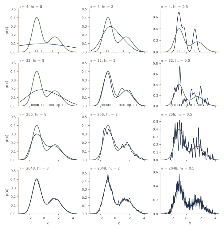
The table and the figure tell the same story. With few samples the middle constant wins: \(h_1 = 8\) blurs the two bumps into one, and \(h_1 = 0.5\) reproduces the samples rather than the density. As \(n\) grows, the widest constant catches up and, at \(n = 2048\), wins, because \(h_n = h_1/\sqrt{n}\) has shrunk it to a sensible width while the narrow window has become ragged. No single \(h_1\) is best for every \(n\), and the best value depends on the unknown density. The theory below explains why all three columns converge anyway.
Convergence of the mean
For a fixed \(\mathbf{x}\), \(p_n(\mathbf{x})\) is a random variable: it depends on which samples we happened to draw. Let \(\bar{p}_n(\mathbf{x})\) and \(\sigma_n^2(\mathbf{x})\) be its mean and variance over repeated draws of the data. We say \(p_n(\mathbf{x})\) converges to \(p(\mathbf{x})\) in mean square when
\[\lim_{n\to\infty} \bar{p}_n(\mathbf{x}) = p(\mathbf{x}) \qquad \text{and} \qquad \lim_{n\to\infty} \sigma_n^2(\mathbf{x}) = 0 .\]The mean is one line. The samples are independent draws from \(p\), and the estimate is an average of \(n\) identically distributed terms, so
\[\bar{p}_n(\mathbf{x}) = \mathcal{E}\left[\frac{1}{n}\sum_{i=1}^{n} \delta_n(\mathbf{x} - \mathbf{x}_i)\right] = \int \delta_n(\mathbf{x} - \mathbf{v})\,p(\mathbf{v})\,d\mathbf{v}.\]The expected estimate is the convolution of the true density with the window: \(p\) seen through a blur of width \(h_n\). It does not depend on \(n\) except through \(h_n\). As \(V_n \to 0\) the window \(\delta_n\) collapses to a delta function at the origin and \(\bar{p}_n(\mathbf{x}) \to p(\mathbf{x})\) wherever \(p\) is continuous. The bias \(\bar{p}_n(\mathbf{x}) - p(\mathbf{x})\) is the price of blurring: negative at peaks, which get flattened, positive in valleys, which get filled in.
For a Gaussian window and our Gaussian mixture the convolution is available in closed form: blurring \(N(\mu, \sigma^2)\) with a \(N(0, h^2)\) bump gives \(N(\mu, \sigma^2 + h^2)\), so \(\bar{p}_n\) is the same mixture with every variance increased by \(h^2\). That is what mix_pdf(x, extra_var=h**2) computes.
Convergence of the variance
The bias alone would let us take \(h_n \to 0\) for any \(n\), which we know gives a useless comb of spikes. The variance shows why. Because \(p_n(\mathbf{x})\) is a sum of \(n\) independent terms \(\delta_n(\mathbf{x} - \mathbf{x}_i)/n\), its variance is \(n\) times the variance of one term:
\[\begin{aligned} \sigma_n^2(\mathbf{x}) &= n\, \mathcal{E}\!\left[\left(\frac{1}{n}\delta_n(\mathbf{x} - \mathbf{x}_i) - \frac{1}{n}\bar{p}_n(\mathbf{x})\right)^{2}\right] \\ &= \frac{1}{n}\int \delta_n^2(\mathbf{x} - \mathbf{v})\,p(\mathbf{v})\,d\mathbf{v} - \frac{1}{n}\bar{p}_n^{\,2}(\mathbf{x}) \\ &= \frac{1}{nV_n}\int \frac{1}{V_n}\varphi^2\!\left(\frac{\mathbf{x} - \mathbf{v}}{h_n}\right) p(\mathbf{v})\,d\mathbf{v} - \frac{1}{n}\bar{p}_n^{\,2}(\mathbf{x}). \end{aligned}\]Drop the last term (it is subtracted, so dropping it gives an upper bound) and bound one factor of \(\varphi\) by its largest value; what remains is the convolution for the mean again:
\[\sigma_n^2(\mathbf{x}) \le \frac{\sup_{\mathbf{u}} \varphi(\mathbf{u})\; \bar{p}_n(\mathbf{x})}{nV_n}.\]This is the key inequality. Small variance wants a large \(V_n\) — broad windows average over many samples — but because the numerator stays bounded, the variance still goes to zero as long as \(nV_n \to \infty\). Together with the bias argument, the following conditions are sufficient for mean-square convergence at every point where \(p\) is continuous: the window is bounded, \(\sup \varphi < \infty\); it decays faster than \(\lVert \mathbf{u} \rVert^{-d}\), so \(\lim_{\lVert \mathbf{u} \rVert \to \infty} \varphi(\mathbf{u}) \prod_{j=1}^{d} u_j = 0\); and the volumes satisfy
\[\lim_{n\to\infty} V_n = 0 \qquad \text{and} \qquad \lim_{n\to\infty} nV_n = \infty .\]The volume must shrink, but more slowly than \(1/n\). Choices such as \(V_n = V_1/\sqrt{n}\) or \(V_n = V_1/\ln n\) qualify. DHS §4.3.1–4.3.2 give the argument in the same form; Problem 1 there asks for the details.
For a Gaussian window in one dimension, the variance formula can also be evaluated exactly. Squaring a \(N(0, h^2)\) bump gives \(\frac{1}{2\sqrt{\pi}\,h}\) times a \(N(0, h^2/2)\) bump, so
\[\sigma_n^2(x) = \frac{1}{n}\left[\frac{1}{2\sqrt{\pi}\,h}\, p_{h^2/2}(x) - p_{h^2}^2(x)\right],\]where \(p_{s}\) is our mixture with every component variance increased by \(s\). The next cell compares the exact bias and variance at the left peak \(x_0 = -1\) with a Monte Carlo estimate over 4000 data sets of \(n = 50\) points, and checks the upper bound (for the Gaussian window \(\sup\varphi = 1/\sqrt{2\pi}\)).
def parzen_bias_var(x, h, n):
    mean = mix_pdf(x, h**2)                                          # convolution p * delta_n
    var = (mix_pdf(x, h**2 / 2) / (2 * np.sqrt(np.pi) * h) - mean**2) / n
    return mean - mix_pdf(x), var

n, reps, x0 = 50, 4000, -1.0
rng_bv = np.random.default_rng(403)
data = np.stack([mix_sample(n, rng_bv) for _ in range(reps)])        # (reps, n)
print("   h     bias     var(exact)  var(MC)    bound      MSE")
for h in [0.05, 0.15, 0.3, 0.6, 1.0]:
    est = np.exp(-0.5 * ((x0 - data) / h)**2).sum(1) / (n * h * np.sqrt(2 * np.pi))
    bias, var = parzen_bias_var(x0, h, n)
    bound = mix_pdf(x0, h**2) / np.sqrt(2 * np.pi) / (n * h)
    print(f"{h:5.2f}  {bias:8.4f}  {var:10.5f}  {est.var():9.5f}  {bound:8.5f}  {bias**2 + var:8.5f}")
print(f"MC mean at h = 1.0: {est.mean():.4f}   exact mean: {mix_pdf(x0, 1.0):.4f}")
   h     bias     var(exact)  var(MC)    bound      MSE
 0.05   -0.0013     0.04214    0.04222   0.06405   0.04214
 0.15   -0.0116     0.01186    0.01182   0.02081   0.01200
 0.30   -0.0406     0.00454    0.00450   0.00963   0.00619
 0.60   -0.1104     0.00142    0.00140   0.00389   0.01360
 1.00   -0.1763     0.00050    0.00050   0.00181   0.03160
MC mean at h = 1.0: 0.2262   exact mean: 0.2264
The exact variance agrees with the Monte Carlo variance to within sampling noise, and the bound holds with room to spare for wide windows (where the dropped \(\bar{p}_n^2/n\) term matters). The bias column grows in magnitude with \(h\) as the peak is flattened, the variance column falls, and their sum, the mean squared error, is smallest at an intermediate width. This is the bias–variance trade-off in its plainest form; module 09 returns to it for classifiers in general.
Now let \(h\) shrink with \(n\). The next cell evaluates the exact bias and variance at \(x_0\) for \(h_n = 0.8/\sqrt{n}\), which satisfies both conditions, and for \(h_n = 8/n\), which shrinks too fast: \(nV_n\) stays at 8.
print("       n    h=0.8/sqrt(n): bias      var      |  h=8/n: bias      var")
for n in [10, 100, 1000, 10000, 100000]:
    b1, v1 = parzen_bias_var(x0, 0.8 / np.sqrt(n), n)
    b2, v2 = parzen_bias_var(x0, 8.0 / n, n)
    print(f"{n:8d}   {b1:12.5f} {v1:10.6f}   | {b2:12.5f} {v2:10.6f}")
       n    h=0.8/sqrt(n): bias      var      |  h=8/n: bias      var
      10       -0.03030   0.029238   |     -0.14796   0.004080
     100       -0.00340   0.012545   |     -0.00340   0.012545
    1000       -0.00034   0.004326   |     -0.00003   0.014037
   10000       -0.00003   0.001404   |     -0.00000   0.014183
  100000       -0.00000   0.000447   |     -0.00000   0.014198
With \(h_n \propto 1/\sqrt{n}\) both bias and variance go to zero. With \(h_n \propto 1/n\) the bias vanishes even faster, but the variance levels off at a positive constant: the estimate keeps jumping around from one data set to the next no matter how much data we collect.
Note. The convergence theorem is reassuring but says nothing about which \(h_1\) to use for the \(n\) we actually have. Without further knowledge of \(p\) beyond continuity, the theory gives no basis for optimizing finite-sample performance. In practice the width is chosen from the data, as in the section on choosing the window below.
How much data: the curse of dimensionality
The examples so far are one-dimensional. In \(d\) dimensions the same local-averaging idea needs far more data. A hypercube that captures a fraction \(f\) of points spread uniformly over the unit cube needs edge length \(f^{1/d}\), so a “local” window quickly stops being local:
print(" d    edge for 1%   edge for 10%")
for d in [1, 2, 5, 10, 50]:
    print(f"{d:2d}   {0.01**(1 / d):10.3f}   {0.1**(1 / d):10.3f}")
 d    edge for 1%   edge for 10%
 1        0.010        0.100
 2        0.100        0.316
 5        0.398        0.631
10        0.631        0.794
50        0.912        0.955
In ten dimensions a window holding 1% of the data spans more than half the range of every coordinate, so it averages over most of the space. To keep windows small and counts large at the same time, the number of samples must grow exponentially with \(d\). This is the curse of dimensionality that module 03 met for parametric models; for nonparametric methods it bites harder, because they assume nothing that could stand in for missing data. The only real remedy is correct prior knowledge — fewer features, or structure such as the smoothness or invariances we build into metrics later in this module.
Classification with Parzen windows
A Parzen classifier estimates each class-conditional density separately, from that class’s samples, and applies the Bayes rule of module 02. With \(n_i\) of the \(n\) samples in class \(\omega_i\) and the class fractions \(n_i/n\) as prior estimates, the discriminant functions are
\[g_i(\mathbf{x}) = p_n(\mathbf{x} \mid \omega_i)\,\hat{P}(\omega_i) = \frac{1}{n_i}\sum_{\mathbf{x}_j \in \omega_i} \delta_n(\mathbf{x} - \mathbf{x}_j) \cdot \frac{n_i}{n} = \frac{1}{n}\sum_{\mathbf{x}_j \in \omega_i} \delta_n(\mathbf{x} - \mathbf{x}_j),\]and we pick the class with the largest \(g_i(\mathbf{x})\). With estimated priors the rule is refreshingly direct: add up the window contributions of each class’s samples and take the biggest total. Known priors that differ from the class fractions enter as \(p_n(\mathbf{x} \mid \omega_i)P(\omega_i)\) instead.
Our running two-dimensional problem has two classes, each an equal mixture of two round Gaussian blobs placed on the corners of a square, so that the classes interleave like a checkerboard: \(\omega_1\) has blobs at \((0, 0)\) and \((2.2, 2.2)\) with standard deviations 0.55 and 0.75, \(\omega_2\) has blobs at \((2.2, 0)\) and \((0, 2.2)\), both with standard deviation 0.65, and the priors are equal. No linear or single-Gaussian model can fit it, and because we know the densities we can compute the Bayes error by numerical integration on a fine grid. In code the classes are labeled 0 and 1 for \(\omega_1\) and \(\omega_2\).
CLS_MU = [np.array([[0.0, 0.0], [2.2, 2.2]]), np.array([[2.2, 0.0], [0.0, 2.2]])]
CLS_SD = [np.array([0.55, 0.75]), np.array([0.65, 0.65])]

def class_logpdf(X, i):
    """ln p(x | w_i) for the two-blob mixture of class i."""
    mu, sd = CLS_MU[i], CLS_SD[i]
    d2 = ((X[:, None, :] - mu[None]) ** 2).sum(-1)
    return logsumexp(-d2 / (2 * sd**2) - np.log(2 * np.pi * sd**2) + np.log(0.5), axis=1)

def sample_two_class(n_per_class, rng):
    X, y = [], []
    for i in range(2):
        comp = rng.integers(0, 2, size=n_per_class)
        X.append(CLS_MU[i][comp] + CLS_SD[i][comp][:, None] * rng.standard_normal((n_per_class, 2)))
        y.append(np.full(n_per_class, i))
    return np.vstack(X), np.concatenate(y)

# Bayes error and true posteriors on a fine grid (equal priors)
gg = np.linspace(-3, 5.2, 411)
GX, GY = np.meshgrid(gg, gg)
Q = np.column_stack([GX.ravel(), GY.ravel()])
dA = (gg[1] - gg[0])**2
joint = 0.5 * np.exp(np.column_stack([class_logpdf(Q, 0), class_logpdf(Q, 1)]))   # p(x, w_i)
p_grid = joint.sum(1)
post_grid = joint / p_grid[:, None]                                              # P(w_i | x)
P_bayes = np.minimum(joint[:, 0], joint[:, 1]).sum() * dA
print(f"total mass on grid {p_grid.sum() * dA:.5f},  Bayes error P* = {P_bayes:.4f}")

X, y = sample_two_class(100, np.random.default_rng(42))        # training set: 100 per class
Xt, yt = sample_two_class(5000, np.random.default_rng(43))     # large test set
total mass on grid 0.99998, Bayes error P* = 0.0863
The classifier works in log space, so that a test point far from every sample gets a very negative score instead of an underflow to zero.
def parzen_classify(Xq, X, y, h):
    """Gaussian Parzen classifier: argmax_i ln[ p_n(x | w_i) P(w_i) ], priors = class fractions."""
    c, d = int(y.max()) + 1, X.shape[1]
    D2 = sq_dists(Xq, X)
    g = np.empty((len(Xq), c))
    for i in range(c):
        m = y == i
        g[:, i] = (logsumexp(-D2[:, m] / (2 * h**2), axis=1) - np.log(m.sum())
                   - d / 2 * np.log(2 * np.pi * h**2) + np.log(m.mean()))
    return g.argmax(1), g

print("    h    training error   test error")
for h in [0.05, 0.1, 0.2, 0.4, 0.8, 1.6]:
    tr = np.mean(parzen_classify(X, X, y, h)[0] != y)
    te = np.mean(parzen_classify(Xt, X, y, h)[0] != yt)
    print(f"{h:5.2f}   {tr:12.3f}   {te:12.4f}")
    h    training error   test error
 0.05          0.000         0.1307
 0.10          0.010         0.1292
 0.20          0.025         0.1118
 0.40          0.060         0.1007
 0.80          0.075         0.1018
 1.60          0.095         0.1111
As \(h\) shrinks, each training point is dominated by its own window and the training error falls to zero. The test error tells a different story: it is worst for the narrowest windows, best in the middle, and rises again when \(h\) is so large that the windows blur the checkerboard. A small training error is no evidence of a good classifier, a theme of module 09. With a good width, the Parzen classifier gets to within about one and a half percentage points of the Bayes error, from only 100 samples per class and without ever being told that the classes are Gaussian mixtures.
The power of the method is its generality: the same code, unchanged, would handle three blobs, a ring, or a spiral. The costs are equally clear. The classifier stores every sample and touches every one of them to classify a single point, and it needs many samples, many more than a correct parametric model would.
Probabilistic neural networks
A probabilistic neural network (PNN) is the Parzen classifier with a Gaussian window, rewritten as a three-layer network so that it can be computed in parallel. Networks are the subject of module 06; this is a preview.
The network has \(d\) input units, one per feature; \(n\) pattern units, one per training sample; and \(c\) category units, one per class. Every input unit connects to every pattern unit through a modifiable weight, and each pattern unit connects to exactly one category unit, the one for its sample’s class.
Training is a single pass. Each training pattern is first normalized to unit length, \(\mathbf{x}_k \leftarrow \mathbf{x}_k/\lVert \mathbf{x}_k \rVert\). The weight vector of pattern unit \(k\) is set equal to it, \(\mathbf{w}_k = \mathbf{x}_k\), and the unit is wired to its class’s category unit. That is all.
Classification. A test pattern \(\mathbf{x}\) is normalized and placed on the inputs. Pattern unit \(k\) forms its net activation, the inner product \(\text{net}_k = \mathbf{w}_k^{t}\mathbf{x}\), and emits \(\exp[(\text{net}_k - 1)/\sigma^2]\), where \(\sigma\) is a width chosen by the user. Each category unit adds up what its pattern units emit, and the network outputs the class with the largest sum.
Why this particular activation function? Work backward from the Gaussian window we want. For unit vectors, \(\lVert \mathbf{x} - \mathbf{w}_k \rVert^2 = \mathbf{x}^{t}\mathbf{x} + \mathbf{w}_k^{t}\mathbf{w}_k - 2\mathbf{w}_k^{t}\mathbf{x} = 2 - 2\,\text{net}_k\), so
\[\exp\!\left[-\frac{\lVert \mathbf{x} - \mathbf{w}_k \rVert^{2}}{2\sigma^{2}}\right] = \exp\!\left[-\frac{2 - 2\,\text{net}_k}{2\sigma^{2}}\right] = \exp\!\left[\frac{\text{net}_k - 1}{\sigma^{2}}\right].\]Each pattern unit therefore emits an unnormalized Gaussian window of width \(\sigma\) centered on its stored pattern, and each category unit computes, up to a constant factor shared by all classes, \(g_i(\mathbf{x})\) from the Parzen classifier above. The normalization is what lets a plain inner product stand in for a distance. (It also discards the length of \(\mathbf{x}\); if length carries information, append a constant feature before normalizing.)
The cell below builds a PNN on three classes of three-dimensional patterns, normalizes them, and checks that the category-unit outputs are the Parzen class sums \(\sum_{\mathbf{x}_j \in \omega_i}\exp(-\lVert \mathbf{x} - \mathbf{x}_j \rVert^2/2\sigma^2)\), and that the decisions agree.
def pnn_train(X, y, c):
    W = X / np.linalg.norm(X, axis=1, keepdims=True)    # w_k = normalized x_k
    A = np.eye(c)[y]                                     # a_ki = 1 if pattern k is in class i
    return W, A

def pnn_classify(Xq, W, A, sigma):
    Xq = Xq / np.linalg.norm(Xq, axis=1, keepdims=True)
    net = Xq @ W.T                                       # net_k = w_k^t x for every pattern unit
    g = np.exp((net - 1) / sigma**2) @ A                 # category units sum their pattern units
    return g.argmax(1), g

rng_pnn = np.random.default_rng(404)
centers = np.array([[1.0, 0.2, 0.3], [0.3, 1.0, 0.4], [0.4, 0.3, 1.0]])
Xp = np.vstack([m + 0.25 * rng_pnn.standard_normal((40, 3)) for m in centers])
yp = np.repeat(np.arange(3), 40)
Xq_p = np.vstack([m + 0.25 * rng_pnn.standard_normal((300, 3)) for m in centers])
yq_p = np.repeat(np.arange(3), 300)

sigma = 0.15
W, A = pnn_train(Xp, yp, 3)
lab_pnn, g_pnn = pnn_classify(Xq_p, W, A, sigma)

Xn = Xp / np.linalg.norm(Xp, axis=1, keepdims=True)      # Parzen sums on the normalized patterns
Xqn = Xq_p / np.linalg.norm(Xq_p, axis=1, keepdims=True)
K = np.exp(-sq_dists(Xqn, Xn) / (2 * sigma**2))
g_parzen = np.stack([K[:, yp == i].sum(1) for i in range(3)], axis=1)
print(f"max relative difference of category outputs: {np.max(np.abs(g_pnn - g_parzen) / g_parzen):.2e}")
print(f"decisions identical: {np.array_equal(lab_pnn, g_parzen.argmax(1))}")
print(f"PNN test error: {np.mean(lab_pnn != yq_p):.4f}")
max relative difference of category outputs: 2.01e-14
decisions identical: True
PNN test error: 0.0644
The two computations agree to rounding error. The appeal of the PNN is practical. Training is one pass with no iteration, and adding a new training pattern later means adding one pattern unit. Storage is \(O((n+1)d)\) weights, which can be large. In a parallel implementation every pattern unit works at once, so classification takes \(O(1)\) time; on a serial computer it is the same \(O(nd)\) scan as any Parzen classifier.
Choosing the window
The width, and more generally the shape and orientation of the window, remain free. The theory only says that the width should shrink slowly as \(n\) grows; the finite-sample answer depends on the unknown density, and a width that suits one part of the space may be wrong in another (our two bumps have different widths, and so would prefer different windows).
The standard answer is to let held-out data decide, the approach module 09 develops as cross-validation. For a density estimate, a natural criterion is the leave-one-out log-likelihood: estimate the density at each sample from the other \(n - 1\) samples, and add up the logs,
\[\ell(h) = \sum_{i=1}^{n} \ln p_{n-1}^{(-i)}(\mathbf{x}_i), \qquad p_{n-1}^{(-i)}(\mathbf{x}_i) = \frac{1}{n-1}\sum_{j \ne i} \delta_n(\mathbf{x}_i - \mathbf{x}_j).\]Leaving the point out matters: with it included, \(\ell(h)\) would grow without bound as \(h \to 0\). For a classifier, choose the width with the smallest error on a validation set. The next cell does both. It also shows the width given by a common rule of thumb for Gaussian windows in one dimension, \(h \approx 1.06\,\hat{\sigma}\,n^{-1/5}\), which is optimal when the data are themselves Gaussian.
def loo_loglik(x, h):
    """Leave-one-out log-likelihood of a 1-D Gaussian Parzen estimate."""
    D2 = (x[:, None] - x[None, :])**2
    np.fill_diagonal(D2, np.inf)                         # leave x_i out of its own estimate
    return np.sum(logsumexp(-D2 / (2 * h**2), axis=1) - np.log((len(x) - 1) * h * np.sqrt(2 * np.pi)))

x200 = mix_sample(200, np.random.default_rng(405))
hs = np.geomspace(0.03, 2.0, 40)
ll = np.array([loo_loglik(x200, h) for h in hs])
h_loo = hs[ll.argmax()]
h_rot = 1.06 * x200.std() * len(x200)**(-1 / 5)
for name, h in [("leave-one-out", h_loo), ("rule of thumb", h_rot)]:
    print(f"{name:14s} h = {h:.3f}   ISE = {ise(parzen(xs[:, None], x200[:, None], h)):.5f}")

Xv, yv = sample_two_class(100, np.random.default_rng(44))      # validation set for the classifier
hs_c = [0.05, 0.1, 0.2, 0.3, 0.4, 0.6, 0.8, 1.2]
val_err = [np.mean(parzen_classify(Xv, X, y, h)[0] != yv) for h in hs_c]
h_best = hs_c[int(np.argmin(val_err))]
print("validation errors:", np.round(val_err, 3))
print(f"chosen h = {h_best},  test error {np.mean(parzen_classify(Xt, X, y, h_best)[0] != yt):.4f}")
leave-one-out  h = 0.443   ISE = 0.00547
rule of thumb  h = 0.540   ISE = 0.00901
validation errors: [0.16  0.155 0.135 0.115 0.135 0.145 0.145 0.145]
chosen h = 0.3,  test error 0.1042
The rule of thumb assumes a single Gaussian, so on our two-bump density it oversmooths; leave-one-out adapts to the data and gives a clearly smaller integrated squared error. The validation set (only 200 points, so its error estimates are coarse) picks \(h = 0.3\), a little narrower than the best widths in the test-error table of the previous section, and its test error is within half a percentage point of the best there.
k-nearest-neighbor estimation
Letting the data set the volume
A fixed window width is a compromise across the whole space. The alternative is to fix the count instead and let the data choose the volume: center a cell on \(\mathbf{x}\) and grow it until it captures \(k_n\) samples, the \(k_n\) nearest neighbors of \(\mathbf{x}\). (In this context the stored samples are often called prototypes.) With \(V_n\) the volume of that cell, the estimate is again
\[p_n(\mathbf{x}) = \frac{k_n/n}{V_n}.\]Where the density is high, the cell stays small and the estimate has fine resolution; where it is low, the cell grows until it reaches enough samples. For a spherical cell of radius \(r\) in \(d\) dimensions the volume is \(V = \pi^{d/2} r^{d}/\Gamma(d/2 + 1)\).
The conditions for convergence are the ones from the start of the module, now stated for the count: \(k_n \to \infty\) makes \(k_n/n\) a reliable estimate of the probability of the cell, and \(k_n/n \to 0\) makes the cell shrink to a point. These two conditions are necessary and sufficient for \(p_n(\mathbf{x})\) to converge in probability to \(p(\mathbf{x})\) at every point where \(p\) is continuous (DHS Problem 5 asks for the proof). With \(k_n = \sqrt{n}\), and \(p_n\) close to \(p\), the volume behaves like \(V_n \approx 1/(\sqrt{n}\,p(\mathbf{x}))\): the same \(1/\sqrt{n}\) rate as the Parzen example, but with a constant set by the local density instead of by us.
def ball_volume(r, d):
    return np.exp(d / 2 * np.log(np.pi) - gammaln(d / 2 + 1)) * r**d

def knn_density(Xq, X, k):
    """k-NN density estimate (k/n) / V, V = volume of the ball reaching the k-th nearest sample."""
    D2 = sq_dists(np.atleast_2d(Xq), X)
    r = np.sqrt(np.partition(D2, k - 1, axis=1)[:, k - 1])
    return k / (len(X) * ball_volume(r, X.shape[1]))

# check in 2-D: standard normal at the origin, true density 1/(2 pi)
rng_kd2 = np.random.default_rng(406)
est = [knn_density(np.zeros((1, 2)), rng_kd2.standard_normal((20000, 2)), 400)[0] for _ in range(10)]
print(f"2-D k-NN estimate at 0 (k = 400, n = 20000), 10 data sets: {np.mean(est):.4f} ± {np.std(est):.4f}"
      f"   true {1 / (2 * np.pi):.4f}")

# the tails decay like k / (2 n |x|), so the integral grows with the range like (k/n) ln L
x16 = mix_sample(16, np.random.default_rng(417))[:, None]
for L in [10, 100, 1000, 10000]:
    tail = np.geomspace(5, L, 4000)
    grid = np.concatenate([-tail[::-1], np.linspace(-5, 5, 20001)[1:-1], tail])
    integral = np.trapezoid(knn_density(grid[:, None], x16, 4), grid)
    print(f"n = 16, k = 4: integral over [-{L}, {L}] = {integral:.3f}")
print(f"(k/n) ln 10 = {4 / 16 * np.log(10):.3f}")
2-D k-NN estimate at 0 (k = 400, n = 20000), 10 data sets: 0.1548 ± 0.0068   true 0.1592
n = 16, k = 4: integral over [-10, 10] = 1.865
n = 16, k = 4: integral over [-100, 100] = 2.474
n = 16, k = 4: integral over [-1000, 1000] = 3.053
n = 16, k = 4: integral over [-10000, 10000] = 3.629
(k/n) ln 10 = 0.576
In the two-dimensional check the average over data sets lands close to the true value, and the spread from one data set to the next is about 5%, as the relative standard deviation \(1/\sqrt{k} = 0.05\) of the count predicts. The second part shows a basic defect: the \(k_n\)-nearest-neighbor estimate is not a density. Far from the data the \(k\)th neighbor is at distance about \(\lvert x \rvert\), so in one dimension the estimate decays only like \(k/(2n\lvert x \rvert)\), and each tenfold increase in the range adds about \((k/n)\ln 10\) to the integral, without end. With \(n = 1\) and \(k = 1\) it is worse still: the estimate is \(1/(2\lvert x - x_1 \rvert)\), which is not even integrable near the sample. The compensation is that the estimate is never zero: no point is ever “empty”, however far it is from the samples. For classification, where only the relative sizes of estimates at the same \(\mathbf{x}\) matter, that can be worth more than a proper normalization.
Relation to Parzen windows
The \(k_n\)-nearest-neighbor estimate is a Parzen estimate with a uniform (ball-shaped) window whose width is not fixed but depends on \(\mathbf{x}\) through the data. Both families need a parameter tuned from data — \(h_1\) for Parzen, \(k_1\) in \(k_n = k_1\sqrt{n}\) for nearest neighbors — and neither choice can be justified in advance. The estimates also look different: the \(k_n\)-nearest-neighbor estimate is continuous, but its slope jumps, and the jumps sit at points midway between samples, where the identity of the \(k\)th neighbor changes, rather than at the samples themselves.
The cell compares the two on the running mixture, using \(k_n = \sqrt{n}\) and a Parzen width chosen by leave-one-out for each \(n\), averaged over 8 data sets. Because the \(k_n\)-nearest-neighbor estimate has infinite integral, we measure error only on \([-3, 4]\), where the density lives.
inside = (xs >= -3) & (xs <= 4)
def ise_inside(p_hat):
    return np.trapezoid((p_hat[inside] - p_x[inside])**2, xs[inside])

rng_cmp = np.random.default_rng(407)
hs_cmp = np.geomspace(0.05, 1.0, 10)
print("    n     Parzen (LOO h)   k-NN (k = sqrt n)")
for n in [16, 64, 256, 1024]:
    e = np.zeros(2)
    for rep in range(8):
        x = mix_sample(n, rng_cmp)
        h = hs_cmp[np.argmax([loo_loglik(x, h) for h in hs_cmp])]
        e += [ise_inside(parzen(xs[:, None], x[:, None], h)),
              ise_inside(knn_density(xs[:, None], x[:, None], int(round(np.sqrt(n)))))]
    print(f"{n:5d}   {e[0] / 8:12.5f}   {e[1] / 8:14.5f}")
    n     Parzen (LOO h)   k-NN (k = sqrt n)
   16        0.03061          0.27770
   64        0.01260          0.05158
  256        0.00342          0.01609
 1024        0.00204          0.00950
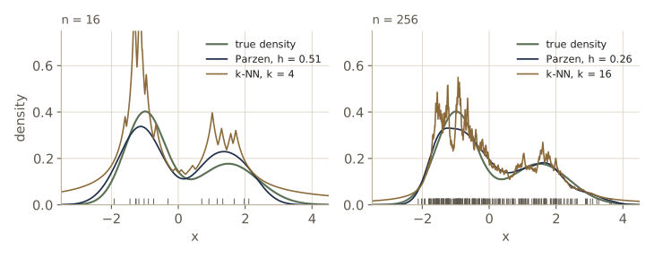
On this smooth density the tuned Parzen estimate is more accurate at every \(n\); the \(k_n\)-nearest-neighbor estimate pays for its spikes and heavy tails. Its adaptivity matters more in higher dimensions and for densities whose scale varies from place to place, where no single width fits.
Estimating posterior probabilities
For classification we do not need the densities themselves, only the posteriors. Place a cell of volume \(V\) around \(\mathbf{x}\) and suppose it captures \(k\) labeled samples, \(k_i\) of them from class \(\omega_i\). The natural estimate of the joint density is \(p_n(\mathbf{x}, \omega_i) = (k_i/n)/V\), and so
\[P_n(\omega_i \mid \mathbf{x}) = \frac{p_n(\mathbf{x}, \omega_i)}{\sum_{j=1}^{c} p_n(\mathbf{x}, \omega_j)} = \frac{k_i}{k}.\]The volume cancels. The estimated posterior is just the fraction of the samples in the cell that carry label \(\omega_i\), and the minimum-error decision is a vote: pick the class most common in the cell. The cell can be sized either way — Parzen style, with \(V_n\) fixed as a function of \(n\), or nearest-neighbor style, grown to hold \(k\) samples. As \(n \to \infty\) with \(k \to \infty\) and \(k/n \to 0\), the estimate converges to the true posterior and the decisions become Bayes-optimal.
The cell below measures how well \(k_i/k\) tracks the true posterior \(P(\omega_2 \mid \mathbf{x})\) of our running problem, as a root-mean-square error weighted by \(p(\mathbf{x})\) (a sample of test points does the weighting), for two training-set sizes. Classifying queries in blocks keeps the distance matrices small.
def knn_votes(Xq, X, y, k, c=2, block=1000):
    """Fraction of each class among the k nearest training samples: the posterior estimate k_i / k."""
    F = np.empty((len(Xq), c))
    for s in range(0, len(Xq), block):
        D2 = sq_dists(Xq[s:s + block], X)
        nn = np.argpartition(D2, k - 1, axis=1)[:, :k] if k > 1 else D2.argmin(1)[:, None]
        F[s:s + block] = np.stack([(y[nn] == i).mean(1) for i in range(c)], axis=1)
    return F

Xe = Xt[::5]                                               # 2000 evaluation points drawn from p(x)
post_e = np.exp(class_logpdf(Xe, 1)) / (np.exp(class_logpdf(Xe, 0)) + np.exp(class_logpdf(Xe, 1)))
X_big, y_big = sample_two_class(1000, np.random.default_rng(45))
print("   k    RMS error, n = 200    n = 2000")
for k in [1, 5, 15, 45, 135]:
    r_small = np.sqrt(np.mean((knn_votes(Xe, X, y, k)[:, 1] - post_e)**2))
    r_big = np.sqrt(np.mean((knn_votes(Xe, X_big, y_big, k)[:, 1] - post_e)**2))
    print(f"{k:4d}   {r_small:14.4f}   {r_big:12.4f}")
   k    RMS error, n = 200    n = 2000
   1           0.2384         0.2434
   5           0.1270         0.1109
  15           0.0927         0.0662
  45           0.1437         0.0420
 135           0.4751         0.0438
With few neighbors the estimate is a noisy fraction; with too many, the neighbors reach into regions where the posterior is different. The best \(k\) is larger for the larger training set, and the error there is smaller — the compromise that the conditions \(k \to \infty\), \(k/n \to 0\) describe. The surprise of the next section is that even the noisiest choice, \(k = 1\), gives a classifier with a provably good error rate.
The nearest-neighbor rule
The rule and its Voronoi cells
Let \(\mathcal{D}^n = \{\mathbf{x}_1, \dots, \mathbf{x}_n\}\) be a set of \(n\) labeled prototypes, and let \(\mathbf{x}' \in \mathcal{D}^n\) be the prototype closest to a test point \(\mathbf{x}\). The nearest-neighbor rule assigns \(\mathbf{x}\) the label of \(\mathbf{x}'\). It is the \(k = 1\) case of the voting rule above, and it needs no training at all beyond storing the data.
Geometrically, the rule divides the space into cells, one per prototype, each containing the points closer to that prototype than to any other. This partition is the Voronoi tessellation of the prototypes. Every point of a cell receives its prototype’s label, so the decision boundary is made of pieces of the perpendicular bisectors between neighboring prototypes of different classes. Each Voronoi cell is convex, since it is an intersection of half-spaces.
The rule is not optimal: with finite or infinite data its error is generally above the Bayes error \(P^*\). But a heuristic already suggests it is not far off. The label \(\theta'\) of the nearest neighbor is a random variable, equal to \(\omega_i\) with probability \(P(\omega_i \mid \mathbf{x}')\). With many prototypes \(\mathbf{x}'\) is very close to \(\mathbf{x}\), so that probability is nearly \(P(\omega_i \mid \mathbf{x})\), the probability that nature’s label at \(\mathbf{x}\) is \(\omega_i\). The rule matches probabilities with nature. Where one class dominates, \(P(\omega_m \mid \mathbf{x}) \approx 1\), the neighbor almost always carries that class and the rule almost always agrees with the Bayes decision. Where all classes are about equally likely, the rule and the Bayes decision often disagree, but then both err with probability close to \(1 - 1/c\) anyway.
Here \(\omega_m(\mathbf{x})\) denotes the class with the largest posterior at \(\mathbf{x}\), the one the Bayes rule picks, so the Bayes conditional error is \(P^*(e \mid \mathbf{x}) = 1 - P(\omega_m \mid \mathbf{x})\) and \(P^* = \int P^*(e \mid \mathbf{x})\,p(\mathbf{x})\,d\mathbf{x}\) (module 02).
def knn_classify(Xq, X, y, k, c=2):
    """k-nearest-neighbor rule: majority vote among the k nearest prototypes (k odd, c = 2)."""
    return knn_votes(Xq, X, y, k, c).argmax(1)

print("  k   training error   test error")
for k in [1, 3, 7, 15, 31]:
    tr, te = np.mean(knn_classify(X, X, y, k) != y), np.mean(knn_classify(Xt, X, y, k) != yt)
    print(f"{k:3d}   {tr:12.3f}   {te:10.4f}")
print(f"Bayes error P* = {P_bayes:.4f}")
  k   training error   test error
  1          0.000       0.1305
  3          0.030       0.1246
  7          0.090       0.1113
 15          0.075       0.1022
 31          0.095       0.1049
Bayes error P* = 0.0863
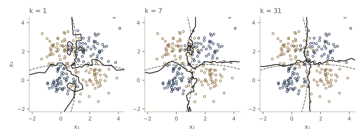
The 1-nearest-neighbor rule classifies its own training set perfectly (each point is its own nearest neighbor) and has a test error well above \(P^*\); voting over more neighbors helps. How much above \(P^*\) can the single-neighbor rule be? The answer requires a large-sample analysis.
Convergence of the nearest neighbor
The error of the rule for a particular test point depends on which prototypes happened to be drawn, through the neighbor \(\mathbf{x}'\). Averaging over the training set gives
\[P(e \mid \mathbf{x}) = \int P(e \mid \mathbf{x}, \mathbf{x}')\,p(\mathbf{x}' \mid \mathbf{x})\,d\mathbf{x}',\]and the overall error is \(P(e) = \int P(e \mid \mathbf{x})\,p(\mathbf{x})\,d\mathbf{x}\). The density \(p(\mathbf{x}' \mid \mathbf{x})\) of the nearest neighbor is hard to write down for finite \(n\), but its limit is easy. Assume \(p\) is continuous and positive at \(\mathbf{x}\). Any ball \(\mathcal{S}\) centered at \(\mathbf{x}\) then has positive probability \(P_{\mathcal{S}} = \int_{\mathcal{S}} p(\mathbf{x}')\,d\mathbf{x}'\). The chance that all \(n\) independent samples miss it is \((1 - P_{\mathcal{S}})^n \to 0\). So however small the ball, the nearest neighbor eventually lies inside it: \(\mathbf{x}'\) converges to \(\mathbf{x}\) in probability, and \(p(\mathbf{x}' \mid \mathbf{x})\) approaches a delta function at \(\mathbf{x}\).
The speed of that convergence depends on the dimension. For \(n\) points spread over a region, the nearest one is at a distance of order \(n^{-1/d}\). The cell measures the average distance from the center of the unit cube to the nearest of \(n\) uniform points:
rng_nn = np.random.default_rng(408)
print("      n     d = 2     d = 10")
for n in [10, 100, 1000, 10000]:
    r = [np.mean([np.sqrt(np.min(((rng_nn.random((n, d)) - 0.5)**2).sum(1))) for _ in range(40)])
         for d in (2, 10)]
    print(f"{n:7d}   {r[0]:.4f}   {r[1]:.4f}")
      n     d = 2     d = 10
     10   0.1761   0.6862
    100   0.0488   0.5276
   1000   0.0156   0.4287
  10000   0.0059   0.3375
In two dimensions a thousandfold increase in data brings the neighbor about thirty times closer; in ten dimensions it only halves. The asymptotic results below are real, but in high dimensions “asymptotic” can mean an astronomical number of samples.
The error rate of the nearest-neighbor rule
To be careful about what is random, write the \(n\) training pairs as \((\mathbf{x}_1, \theta_1), \dots, (\mathbf{x}_n, \theta_n)\), where each label \(\theta_j\) is drawn from the priors and each \(\mathbf{x}_j\) from \(p(\mathbf{x} \mid \theta_j)\), all independently. Nature presents a test pair \((\mathbf{x}, \theta)\); the nearest prototype is \(\mathbf{x}'_n\), with label \(\theta'_n\). The two labels were drawn independently, so given the two positions
\[P(\theta, \theta'_n \mid \mathbf{x}, \mathbf{x}'_n) = P(\theta \mid \mathbf{x})\,P(\theta'_n \mid \mathbf{x}'_n).\]The rule errs exactly when \(\theta \ne \theta'_n\), so
\[P_n(e \mid \mathbf{x}, \mathbf{x}'_n) = 1 - \sum_{i=1}^{c} P(\theta = \omega_i, \theta'_n = \omega_i \mid \mathbf{x}, \mathbf{x}'_n) = 1 - \sum_{i=1}^{c} P(\omega_i \mid \mathbf{x})\,P(\omega_i \mid \mathbf{x}'_n).\]As \(n \to \infty\) the density of \(\mathbf{x}'_n\) collapses onto \(\mathbf{x}\), and if the posteriors are continuous at \(\mathbf{x}\) the average over \(\mathbf{x}'_n\) becomes evaluation at \(\mathbf{x}\):
\[\lim_{n\to\infty} P_n(e \mid \mathbf{x}) = 1 - \sum_{i=1}^{c} P^{2}(\omega_i \mid \mathbf{x}).\]Averaging over \(\mathbf{x}\) (and assuming the limit and the integral can be exchanged) gives the asymptotic error rate:
Result. With unlimited prototypes, the error rate of the nearest-neighbor rule is
\[P = \lim_{n\to\infty} P_n(e) = \int \left[1 - \sum_{i=1}^{c} P^{2}(\omega_i \mid \mathbf{x})\right] p(\mathbf{x})\,d\mathbf{x}.\]
This is an exact formula, and for our running problem we can evaluate it on the grid. The cell compares it with the simulated error of the nearest-neighbor rule for growing training sets, averaged over five training sets each.
P_nn = np.sum((1 - (post_grid**2).sum(1)) * p_grid) * dA
print(f"Bayes P* = {P_bayes:.4f}   asymptotic NN error P = {P_nn:.4f}   (2P* = {2 * P_bayes:.4f})")
rng_sim = np.random.default_rng(409)
Xs, ys = Xt[::2], yt[::2]                                  # 5000 test points
print("  n per class   simulated NN error")
for n in [10, 40, 160, 640, 2560]:
    errs = []
    for rep in range(5):
        Xn_, yn_ = sample_two_class(n, rng_sim)
        errs.append(np.mean(knn_classify(Xs, Xn_, yn_, 1) != ys))
    print(f"{n:10d}   {np.mean(errs):12.4f} ± {np.std(errs):.4f}")
Bayes P* = 0.0863   asymptotic NN error P = 0.1259   (2P* = 0.1726)
  n per class   simulated NN error
        10         0.1578 ± 0.0285
        40         0.1437 ± 0.0050
       160         0.1374 ± 0.0053
       640         0.1349 ± 0.0065
      2560         0.1352 ± 0.0042
The finite-sample error falls toward the asymptotic value, but slowly: with 2560 samples per class it is still about one percentage point above it, because the nearest neighbor is not yet close enough for \(P(\omega_i \mid \mathbf{x}'_n)\) to equal \(P(\omega_i \mid \mathbf{x})\) near the boundary. The asymptotic error itself sits between \(P^*\) and \(2P^*\), as the next section proves it must.
Error bounds: the Cover–Hart theorem
The exact formula depends on the whole posterior function. A cleaner statement bounds \(P\) in terms of the single number \(P^*\). The lower bound is quick: at each \(\mathbf{x}\), \(\sum_i P^2(\omega_i \mid \mathbf{x}) \le P(\omega_m \mid \mathbf{x}) \sum_i P(\omega_i \mid \mathbf{x}) = P(\omega_m \mid \mathbf{x})\), so the integrand is at least \(1 - P(\omega_m \mid \mathbf{x}) = P^*(e \mid \mathbf{x})\), and \(P \ge P^*\). No rule beats Bayes.
For the upper bound, ask how small \(\sum_i P^2(\omega_i \mid \mathbf{x})\) can be when the Bayes conditional error \(P^*(e \mid \mathbf{x})\) is fixed. Split off the largest term,
\[\sum_{i=1}^{c} P^{2}(\omega_i \mid \mathbf{x}) = P^{2}(\omega_m \mid \mathbf{x}) + \sum_{i \ne m} P^{2}(\omega_i \mid \mathbf{x}),\]where the first term equals \((1 - P^*(e \mid \mathbf{x}))^2\) and the other \(c - 1\) posteriors are nonnegative with sum \(P^*(e \mid \mathbf{x})\). A sum of squares with a fixed total is smallest when the terms are equal (by the Cauchy–Schwarz inequality, \(\sum_{i \ne m} P_i^2 \ge (\sum_{i \ne m} P_i)^2/(c - 1)\)), that is, when each of the other posteriors is \(P^*(e \mid \mathbf{x})/(c - 1)\). Therefore
\[\sum_{i=1}^{c} P^{2}(\omega_i \mid \mathbf{x}) \ge (1 - P^*(e \mid \mathbf{x}))^{2} + \frac{P^{*2}(e \mid \mathbf{x})}{c - 1}, \qquad 1 - \sum_{i=1}^{c} P^{2}(\omega_i \mid \mathbf{x}) \le 2P^*(e \mid \mathbf{x}) - \frac{c}{c - 1}P^{*2}(e \mid \mathbf{x}).\]Integrating against \(p(\mathbf{x})\) and dropping the negative term already gives \(P \le 2P^*\). To keep the negative term we need a lower bound on \(\int P^{*2}(e \mid \mathbf{x})\,p(\mathbf{x})\,d\mathbf{x}\). The variance of \(P^*(e \mid \mathbf{x})\) as \(\mathbf{x}\) varies is nonnegative,
\[\int \left[P^*(e \mid \mathbf{x}) - P^*\right]^{2} p(\mathbf{x})\,d\mathbf{x} = \int P^{*2}(e \mid \mathbf{x})\,p(\mathbf{x})\,d\mathbf{x} - P^{*2} \ge 0,\]so the integral is at least \(P^{*2}\), with equality exactly when \(P^*(e \mid \mathbf{x})\) is the same at every \(\mathbf{x}\). Substituting:
Result (Cover–Hart bounds). For \(c\) classes, the asymptotic nearest-neighbor error \(P\) and the Bayes error \(P^*\) satisfy
\[P^* \le P \le P^*\left(2 - \frac{c}{c - 1}P^*\right).\]
Both bounds are tight: for every \(P^*\) between 0 and \((c-1)/c\) there are distributions that reach them. The upper bound is reached in the zero-information case, where all classes have the same density \(p(\mathbf{x} \mid \omega_i)\), so every posterior equals its prior and the conditional Bayes error is constant; choose the priors \(1 - P^*\) for one class and \(P^*/(c-1)\) for each of the others, and both inequalities in the derivation become equalities. The lower bound is reached when each \(\mathbf{x}\) has either one certain class or all classes equally likely. The two bounds meet at \(P^* = 0\) and at \(P^* = (c-1)/c\), where every rule is guessing.
The practical reading: when the Bayes error is small, \(P \le 2P^*\) almost exactly. With unlimited data, even an arbitrarily clever rule could at most halve the error of the nearest-neighbor rule. Put differently, the single nearest neighbor already carries half or more of everything an unlimited labeled sample can tell us about the class of a point.
To check the theorem, we need problems whose Bayes error we know. The cell builds two families of equal-prior problems with unit-covariance Gaussian classes in two dimensions: two classes whose means are a distance \(\Delta\) apart, and three classes at the corners of an equilateral triangle of side \(\Delta\). For each it computes \(P^*\) and the asymptotic \(P\) on a grid, and simulates the nearest-neighbor rule with 1500 prototypes per class.
def gauss_problem(means, n_train, n_test, rng, ks=(1,), half=6.0, m=361):
    """Bayes error, asymptotic NN error and simulated k-NN errors for unit-variance
    Gaussian classes with equal priors."""
    means = np.asarray(means, float)
    c = len(means)
    lo, hi = means.min(0) - half, means.max(0) + half
    u, v = np.linspace(lo[0], hi[0], m), np.linspace(lo[1], hi[1], m)
    U, V = np.meshgrid(u, v)
    G = np.column_stack([U.ravel(), V.ravel()])
    J = np.exp(-0.5 * sq_dists(G, means)) / (2 * np.pi * c)        # p(x, w_i)
    px, cell = J.sum(1), (u[1] - u[0]) * (v[1] - v[0])
    post = J / np.maximum(px, 1e-300)[:, None]
    P_star = np.sum(px - J.max(1)) * cell
    P_inf = np.sum((1 - (post**2).sum(1)) * px) * cell
    def draw(n):
        return (np.repeat(means, n, axis=0) + rng.standard_normal((c * n, 2)), np.repeat(np.arange(c), n))
    Xtr, ytr = draw(n_train)
    Xte, yte = draw(n_test)
    sims = [np.mean(knn_votes(Xte, Xtr, ytr, k, c).argmax(1) != yte) for k in ks]
    return P_star, P_inf, sims, post, px, cell

def cover_hart_upper(P_star, c):
    return P_star * (2 - c / (c - 1) * P_star)

rng_ch = np.random.default_rng(410)
tri = np.array([[0.0, 0.0], [1.0, 0.0], [0.5, np.sqrt(3) / 2]])
print(" c   Delta    P*      P (asympt.)  P (simulated)  upper bound")
for c, deltas in [(2, [0.3, 0.8, 1.5, 2.5, 3.5]), (3, [0.5, 1.2, 2.0, 3.0, 4.0])]:
    for D in deltas:
        means = [[0, 0], [D, 0]] if c == 2 else D * tri
        Ps, Pi, (Psim,), *_ = gauss_problem(means, 1500, 1500, rng_ch)
        ok = Ps <= Pi <= cover_hart_upper(Ps, c)
        print(f"{c:2d}  {D:5.1f}  {Ps:.4f}   {Pi:.4f}      {Psim:.4f}"
              f"        {cover_hart_upper(Ps, c):.4f}   {ok}")

# zero-information case: identical class densities, priors (1 - P*, P*/2, P*/2)
Pz = 0.3
priors = np.array([1 - Pz, Pz / 2, Pz / 2])
print(f"zero-information, c = 3, P* = {Pz}: P = {1 - (priors**2).sum():.4f}, "
      f"bound = {cover_hart_upper(Pz, 3):.4f}")
 c   Delta    P*      P (asympt.)  P (simulated)  upper bound
 2    0.3  0.4404   0.4890      0.4807        0.4929   True
 2    0.8  0.3446   0.4303      0.4300        0.4517   True
 2    1.5  0.2267   0.3096      0.3077        0.3506   True
 2    2.5  0.1057   0.1534      0.1573        0.1890   True
 2    3.5  0.0401   0.0599      0.0513        0.0770   True
 3    0.5  0.5623   0.6395      0.6344        0.6503   True
 3    1.2  0.4109   0.5262      0.5324        0.5686   True
 3    2.0  0.2548   0.3524      0.3562        0.4122   True
 3    3.0  0.1153   0.1678      0.1771        0.2107   True
 3    4.0  0.0415   0.0620      0.0604        0.0803   True
zero-information, c = 3, P* = 0.3: P = 0.4650, bound = 0.4650
Every problem satisfies the bounds, and the simulated errors sit close to the asymptotic values (within the noise of a few thousand test points). The Gaussian problems land well below the upper bound because their conditional Bayes error varies a lot from place to place: near the means it is almost zero, near the boundaries it is almost one half. The zero-information case, with a constant conditional error, reaches the bound exactly.
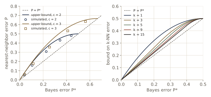
We should be honest about what the theorem does not say. It is an asymptotic statement. For finite \(n\), the only general results are negative: convergence to the limit can be arbitrarily slow, and the error need not even decrease monotonically with \(n\). Useful finite-sample statements need assumptions about the distributions (DHS Problems 13 and 14 explore two examples).
The k-nearest-neighbor rule
The \(k\)-nearest-neighbor rule classifies \(\mathbf{x}\) by a majority vote among the labels of its \(k\) nearest prototypes. We analyze two classes with \(k\) odd, so there are no ties.
Fix \(k\) and let \(n \to \infty\). All \(k\) neighbors converge to \(\mathbf{x}\), so their labels become independent draws with probabilities \(P(\omega_i \mid \mathbf{x})\). Write \(p = P^*(e \mid \mathbf{x})\) for the smaller of the two posteriors. The Bayes rule always picks the majority class \(\omega_m\); the 1-nearest-neighbor rule picks it with probability \(1 - p\); the \(k\)-nearest-neighbor rule picks it whenever at least \((k+1)/2\) of the \(k\) neighbors carry it, which happens with probability
\[\sum_{j=(k+1)/2}^{k} \binom{k}{j} (1-p)^{j} p^{k-j},\]and this grows toward 1 as \(k\) increases. The rule errs if nature’s label is \(\omega_m\) but the vote goes the other way, or nature’s label is the minority class and the vote goes to \(\omega_m\). Adding the two cases and indexing by the number \(i\) of neighbors on the losing side of the vote gives the large-sample conditional error
\[f_k(p) = \sum_{i=0}^{(k-1)/2} \binom{k}{i} \left[p^{\,i+1}(1-p)^{k-i} + p^{\,k-i}(1-p)^{i+1}\right].\]For \(k = 1\) it is \(2p(1-p)\), the two-class nearest-neighbor integrand from before. The asymptotic error is \(P_k = \int f_k(P^*(e \mid \mathbf{x}))\,p(\mathbf{x})\,d\mathbf{x}\). To bound it by a function of \(P^*\) alone, as for \(k = 1\), let \(Q_k\) be the smallest concave function that lies above \(f_k\) on \([0, 1/2]\). Then by Jensen’s inequality for concave functions,
\[P_k \le \int Q_k(P^*(e \mid \mathbf{x}))\,p(\mathbf{x})\,d\mathbf{x} \le Q_k\!\left(\int P^*(e \mid \mathbf{x})\,p(\mathbf{x})\,d\mathbf{x}\right) = Q_k(P^*).\]For \(k = 1\), \(f_1\) is already concave and \(Q_1(P^*) = 2P^*(1-P^*)\), the Cover–Hart bound with \(c = 2\). As \(k\) grows, the vote becomes a better and better estimate of the majority, \(f_k(p) \to p\), and the bounds squeeze down onto \(P^*\): in the limit of large \(k\) (with \(n\) even larger), the rule is optimal. DHS Problem 18 asks you to derive \(f_k\) with every assumption stated.
The cell computes \(f_k\), its concave majorant (the upper convex hull of its graph), and then, for the running problem, the asymptotic error \(P_k\) on the grid, the bound \(Q_k(P^*)\), and the simulated error of the \(k\)-nearest-neighbor rule with 2000 prototypes per class.
from math import comb

def f_knn(p, k):
    """Large-sample conditional error of the k-NN rule (two classes, k odd); p = min posterior."""
    return sum(comb(k, i) * (p**(i + 1) * (1 - p)**(k - i) + p**(k - i) * (1 - p)**(i + 1))
               for i in range((k - 1) // 2 + 1))

def concave_majorant(t, f):
    """Upper hull of the points (t_j, f_j): the smallest concave function above f, on the grid t."""
    hull = []
    for j in range(len(t)):
        while len(hull) >= 2:
            a, b = hull[-2], hull[-1]
            if (f[b] - f[a]) * (t[j] - t[a]) <= (f[j] - f[a]) * (t[b] - t[a]):
                hull.pop()                                  # b lies on or below the chord a-j
            else:
                break
        hull.append(j)
    return np.interp(t, t[hull], f[hull])

pp = np.linspace(0, 0.5, 2001)
Qk = {k: concave_majorant(pp, f_knn(pp, k)) for k in [1, 3, 5, 9, 15]}
print(f"k = 1: max |Q_1 - 2p(1-p)| = {np.max(np.abs(Qk[1] - 2 * pp * (1 - pp))):.2e}")

X2k, y2k = sample_two_class(2000, np.random.default_rng(46))
p_min = post_grid.min(1)                                    # P*(e | x) on the grid
print("  k   asymptotic P_k   simulated (n = 2000/class)   bound Q_k(P*)")
for k in [1, 3, 5, 9, 15]:
    P_k = np.sum(f_knn(p_min, k) * p_grid) * dA
    sim = np.mean(knn_classify(Xs, X2k, y2k, k) != ys)
    print(f"{k:3d}   {P_k:12.4f}   {sim:18.4f}   {np.interp(P_bayes, pp, Qk[k]):16.4f}")
print(f"Bayes error P* = {P_bayes:.4f}")
k = 1: max |Q_1 - 2p(1-p)| = 0.00e+00
  k   asymptotic P_k   simulated (n = 2000/class)   bound Q_k(P*)
  1         0.1259               0.1266             0.1577
  3         0.1035               0.1040             0.1135
  5         0.0971               0.1002             0.1051
  9         0.0925               0.0992             0.0990
 15         0.0901               0.0946             0.0956
Bayes error P* = 0.0863
The asymptotic error falls toward \(P^*\) as \(k\) grows and stays under the bound. The simulated errors follow the asymptotic values closely for small \(k\) but fall behind as \(k\) grows; at \(k = 9\) the finite-sample error has reached the bound itself. That is the finite-sample side of the story. A large \(k\) gives a reliable vote, but all \(k\) neighbors must be close enough to \(\mathbf{x}\) that their posteriors match \(P(\omega_i \mid \mathbf{x})\), and with 2000 samples per class the ninth neighbor is already noticeably farther away than the first. This forces \(k\) to be a small fraction of \(n\); only as \(n \to \infty\) can both demands be met at once.
Computational complexity
The nearest-neighbor rule is simple to state and expensive to run. A naive search for the nearest of \(n\) prototypes in \(d\) dimensions computes \(n\) distances at \(O(d)\) each, so \(O(dn)\) time per query, and stores all \(nd\) numbers. (A parallel circuit with one unit per Voronoi cell could answer in \(O(1)\) time using \(O(n)\) space; DHS Figure 4.17 sketches one.) Three families of tricks reduce the cost: partial distances, prestructuring the prototypes, and editing them.
Partial distance. Accumulate the squared distance one coordinate at a time,
\[D_r(\mathbf{a}, \mathbf{b}) = \left(\sum_{k=1}^{r} (a_k - b_k)^{2}\right)^{1/2}, \qquad r \le d,\]and stop as soon as it exceeds the full distance to the best prototype found so far. Because the partial sum can only grow as coordinates are added, the abandoned prototype could not have been closer, and the search remains exact. The savings depend on how quickly the partial distance becomes large, so it pays to visit high-variance coordinates first.
def nn_partial_distance(x, X):
    """Exact nearest neighbor with early termination; returns (index, number of coordinate operations)."""
    best, best_d2, ops = -1, np.inf, 0
    for j, row in enumerate(X):
        s = 0.0
        for a, b in zip(x, row):
            s += (a - b) * (a - b)
            ops += 1
            if s >= best_d2:
                break                                      # partial distance already too large
        else:
            best, best_d2 = j, s
    return best, ops

rng_pd = np.random.default_rng(411)
d, n = 16, 1000
scales = 2.0 ** (-np.arange(d) / 3)                         # coordinate spreads fall from 1 to about 0.03
Xpd = rng_pd.standard_normal((n, d)) * scales
Qpd = rng_pd.standard_normal((40, d)) * scales
for name, order in [("high variance first", np.arange(d)), ("low variance first", np.arange(d)[::-1])]:
    Xl, ops_total, correct = Xpd[:, order].tolist(), 0, 0
    for q in Qpd:
        j, ops = nn_partial_distance(q[order].tolist(), Xl)
        ops_total += ops
        correct += j == np.argmin(((Xpd - q)**2).sum(1))
    print(f"{name:20s}: {ops_total / (40 * n * d):.3f} of the full n*d operations,"
          f" exact on {correct}/40 queries")
high variance first : 0.117 of the full n*d operations, exact on 40/40 queries
low variance first  : 0.776 of the full n*d operations, exact on 40/40 queries
Prestructuring organizes the prototypes in advance into a search tree so that a query examines only some of them. The crudest version picks a few “entry” prototypes and links every other prototype to its nearest entry; a query finds the closest entry and searches only that entry’s group. For points spread over the unit square with entries at the four quarter points, a query examines about a quarter of the data. But the search is no longer exact: a query near a group boundary can have its true nearest neighbor in the next group.
rng_q = np.random.default_rng(412)
P_uni = rng_q.random((2000, 2))
entries = np.array([[0.25, 0.25], [0.75, 0.25], [0.25, 0.75], [0.75, 0.75]])
group = sq_dists(P_uni, entries).argmin(1)                  # link each prototype to its quadrant
Qu = rng_q.random((2000, 2))
q_group = sq_dists(Qu, entries).argmin(1)
exact = sq_dists(Qu, P_uni).argmin(1)
misses, examined = 0, 0
for q, gq, e in zip(Qu, q_group, exact):
    members = np.flatnonzero(group == gq)
    misses += members[np.argmin(((P_uni[members] - q)**2).sum(1))] != e
    examined += len(members)
print(f"examined {examined / (2000 * 2000):.3f} of the prototypes per query; "
      f"wrong neighbor on {misses / 2000:.1%} of queries")
examined 0.250 of the prototypes per query; wrong neighbor on 1.4% of queries
A proper search tree can keep the search exact by backtracking. The k-d tree splits the prototypes at the median of one coordinate, recursively, until each leaf holds a handful of points. A query descends to the leaf containing it, then climbs back up, visiting the far side of a split only if the splitting plane is closer than the best distance found so far — only then could a closer prototype lie beyond it.
def kd_build(idx, P, leaf_size=8, depth=0):
    if len(idx) <= leaf_size:
        return ("leaf", idx)
    dim = int(np.argmax(P[idx].max(0) - P[idx].min(0)))    # split the widest coordinate
    vals = P[idx, dim]
    cut = np.median(vals)
    left, right = idx[vals <= cut], idx[vals > cut]
    if len(left) == 0 or len(right) == 0:
        return ("leaf", idx)
    return ("node", dim, cut, kd_build(left, P, leaf_size, depth + 1),
            kd_build(right, P, leaf_size, depth + 1))

def kd_nearest(tree, P, q, best=(np.inf, -1), counter=None):
    if tree[0] == "leaf":
        idx = tree[1]
        d2 = ((P[idx] - q)**2).sum(1)
        counter[0] += len(idx)                              # distances actually computed
        j = int(np.argmin(d2))
        return (d2[j], idx[j]) if d2[j] < best[0] else best
    _, dim, cut, left, right = tree
    near, far = (left, right) if q[dim] <= cut else (right, left)
    best = kd_nearest(near, P, q, best, counter)
    if (q[dim] - cut)**2 < best[0]:                         # the other side could hold a closer point
        best = kd_nearest(far, P, q, best, counter)
    return best

rng_kd = np.random.default_rng(413)
for d in [2, 4, 8]:
    P_kd = rng_kd.random((5000, d))
    tree = kd_build(np.arange(5000), P_kd)
    Q_kd = rng_kd.random((200, d))
    counter, correct = [0], 0
    for q in Q_kd:
        _, j = kd_nearest(tree, P_kd, q, counter=counter)
        correct += j == np.argmin(((P_kd - q)**2).sum(1))
    print(f"d = {d}: {counter[0] / 200:7.1f} distances per query (of 5000), exact on {correct}/200")
d = 2:    10.4 distances per query (of 5000), exact on 200/200
d = 4:    45.8 distances per query (of 5000), exact on 200/200
d = 8:   639.7 distances per query (of 5000), exact on 200/200
In two dimensions the tree computes about ten distances instead of 5000, and it is always exact. The advantage fades as \(d\) grows, because in high dimensions nearly every splitting plane is closer than the nearest neighbor, and the search has to visit most of the leaves. This is the curse of dimensionality once more, now as a cost in time.
In practice. Measure before optimizing. For a few thousand prototypes in a few dimensions, one vectorized distance computation per block of queries, as in
knn_votes, is already fast; trees pay off when \(n\) is large and \(d\) is small; and when both are large, editing the prototype set usually helps more than any exact search structure.
Editing (also called pruning or condensing) removes prototypes that do not affect the decisions. DHS’s editing algorithm (§4.5.5, Algorithm 3) keeps exactly the prototypes that have at least one Voronoi neighbor from a different class. A prototype whose Voronoi neighbors all share its label is surrounded by its own class; deleting it hands its cell to those neighbors, which carry the same label, so the decision boundary does not move at all. In two dimensions, two prototypes are Voronoi neighbors exactly when they are joined by an edge of the Delaunay triangulation, which scipy.spatial.Delaunay computes; this is the one place we borrow a geometric routine instead of writing it. The general algorithm is expensive: building a Voronoi diagram in \(d\) dimensions costs roughly \(O(n^{\lfloor d/2 \rfloor})\), which is why cheaper editing rules are popular.
Two classic alternatives aim at different goals. Wilson editing removes every prototype that is misclassified by the \(k\)-nearest-neighbor rule applied to the other prototypes (we use \(k = 3\)). It deletes points on the wrong side of the Bayes boundary, the stray points that give the 1-nearest-neighbor boundary its islands, so it changes the boundary, usually for the better. Hart’s condensing does the opposite kind of job: it starts with a store holding one prototype, then repeatedly sweeps through the data, adding any prototype that the 1-nearest-neighbor rule on the current store misclassifies, until a full sweep adds nothing. The resulting store classifies every original prototype correctly, usually with far fewer points, though not the fewest possible. Condensing keeps noisy points (they are exactly the ones misclassified), each of which pulls a few neighbors into the store with it, so it is usually run after Wilson editing to get a smaller store.
from scipy.spatial import Delaunay

def voronoi_edit(X, y):
    """Keep prototypes with at least one Voronoi (Delaunay) neighbor of another class (2-D)."""
    indptr, nbrs = Delaunay(X).vertex_neighbor_vertices
    return np.array([np.any(y[nbrs[indptr[i]:indptr[i + 1]]] != y[i]) for i in range(len(X))])

def wilson_edit(X, y, k=3):
    """Keep the prototypes that the k-NN rule on all the other prototypes classifies correctly."""
    D2 = sq_dists(X, X)
    np.fill_diagonal(D2, np.inf)                            # a point may not vote for itself
    nn = np.argsort(D2, axis=1)[:, :k]
    votes = np.stack([(y[nn] == i).sum(1) for i in range(int(y.max()) + 1)], axis=1)
    return votes.argmax(1) == y

def hart_condense(X, y, rng):
    """Hart's condensed nearest neighbor: returns the indices of the store."""
    order = rng.permutation(len(X))
    store, changed = [order[0]], True
    while changed:
        changed = False
        for i in order:
            if i in store:
                continue
            j = store[int(np.argmin(((X[store] - X[i])**2).sum(1)))]
            if y[j] != y[i]:                                # misclassified by the store: add it
                store.append(i)
                changed = True
    return np.array(store)

keep_v = voronoi_edit(X, y)
same = np.array_equal(knn_classify(Q[::9], X, y, 1), knn_classify(Q[::9], X[keep_v], y[keep_v], 1))
keep_w = wilson_edit(X, y)
Xw, yw = X[keep_w], y[keep_w]
s_raw = hart_condense(X, y, np.random.default_rng(47))
s_w = hart_condense(Xw, yw, np.random.default_rng(47))
rows = [("all prototypes", X, y), ("Voronoi editing", X[keep_v], y[keep_v]),
        ("Wilson editing", Xw, yw), ("Hart condensing", X[s_raw], y[s_raw]),
        ("Wilson, then Hart", Xw[s_w], yw[s_w])]
for name, Xr, yr in rows:
    err = np.mean(knn_classify(Xt, Xr, yr, 1) != yt)
    print(f"{name:18s} {len(Xr):4d} prototypes   1-NN test error {err:.4f}")
print(f"Voronoi-edited set gives the same decisions on a grid of {len(Q[::9])} points: {same}")
all prototypes      200 prototypes   1-NN test error 0.1305
Voronoi editing      84 prototypes   1-NN test error 0.1305
Wilson editing      181 prototypes   1-NN test error 0.1218
Hart condensing      37 prototypes   1-NN test error 0.1367
Wilson, then Hart    20 prototypes   1-NN test error 0.1527
Voronoi-edited set gives the same decisions on a grid of 18769 points: True
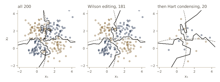
Voronoi editing drops more than half the prototypes, those deep inside each blob, and leaves the decisions exactly as they were. Wilson editing removes the few points that their neighbors outvote, and the test error drops to about that of the 3-nearest-neighbor rule. Condensing is the aggressive step: it cuts the store to a small fraction of the data, and the price is up to a few percentage points of test error. The store is guaranteed to classify the training set correctly, not to reproduce the full decision boundary, and with so few points the boundary between them is only a rough copy (compare the right panel of the figure with the middle one). Which trade is acceptable depends on how much memory and time matter. One drawback of all these methods is that they need the whole training set in advance; a new prototype cannot simply be added later. The methods also combine: edit first, build a search tree on what remains, and use partial distances within the tree’s leaves.
Metrics and nearest-neighbor classification
Everything so far measured closeness with the Euclidean distance. The nearest-neighbor rule works with any notion of distance, and choosing it well is often the most effective way to improve the classifier: the metric is where prior knowledge about the problem enters.
Properties of metrics
A metric \(D(\cdot, \cdot)\) is a function of two patterns that satisfies, for all vectors \(\mathbf{a}\), \(\mathbf{b}\), \(\mathbf{c}\):
- nonnegativity: \(D(\mathbf{a}, \mathbf{b}) \ge 0\);
- reflexivity: \(D(\mathbf{a}, \mathbf{b}) = 0\) if and only if \(\mathbf{a} = \mathbf{b}\);
- symmetry: \(D(\mathbf{a}, \mathbf{b}) = D(\mathbf{b}, \mathbf{a})\);
- triangle inequality: \(D(\mathbf{a}, \mathbf{b}) + D(\mathbf{b}, \mathbf{c}) \ge D(\mathbf{a}, \mathbf{c})\).
The Euclidean distance is the \(k = 2\) member of the Minkowski metric family, also called the \(L_k\) norm of the difference:
\[L_k(\mathbf{a}, \mathbf{b}) = \left(\sum_{j=1}^{d} \lvert a_j - b_j \rvert^{k}\right)^{1/k}.\]\(L_1\) is the Manhattan or city-block distance, the length of a path between \(\mathbf{a}\) and \(\mathbf{b}\) made of segments parallel to the axes. As \(k \to \infty\), \(L_k\) tends to \(L_\infty(\mathbf{a}, \mathbf{b}) = \max_j \lvert a_j - b_j \rvert\), the largest of the coordinate-wise differences. The set of points at distance 1 from the origin is a diamond for \(L_1\), a circle for \(L_2\), and a square for \(L_\infty\). For \(k \ge 1\) the triangle inequality is Minkowski’s inequality; for \(0 < k < 1\) it fails, and the formula is no longer a metric.
For patterns that are sets — the words in a document, the attributes an object has — the Tanimoto metric compares two sets \(\mathcal{S}_1\) and \(\mathcal{S}_2\) with \(n_1\) and \(n_2\) elements, \(n_{12}\) of them shared:
\[D_{\text{Tanimoto}}(\mathcal{S}_1, \mathcal{S}_2) = \frac{n_1 + n_2 - 2n_{12}}{n_1 + n_2 - n_{12}},\]the fraction of the elements in the union that are not in the intersection. It suits problems where two features are either the same or different, with no graded similarity.
def minkowski(a, b, k):
    diff = np.abs(np.asarray(a, float) - np.asarray(b, float))
    return diff.max(-1) if np.isinf(k) else (diff**k).sum(-1)**(1 / k)

def tanimoto(S1, S2):
    n1, n2, n12 = len(S1), len(S2), len(S1 & S2)
    return (n1 + n2 - 2 * n12) / (n1 + n2 - n12)

rng_m = np.random.default_rng(414)
Am, Bm, Cm = (rng_m.standard_normal((20000, 3)) for _ in range(3))
for k in [0.5, 1, 2, 4, np.inf]:
    bad = np.mean(minkowski(Am, Bm, k) + minkowski(Bm, Cm, k) < minkowski(Am, Cm, k) - 1e-12)
    print(f"k = {k:>4}: triangle inequality violated in {bad:.2%} of random triples")
print("k = 0.5 on (0,0), (1,0), (1,1):", minkowski([0, 0], [1, 0], 0.5) + minkowski([1, 0], [1, 1], 0.5),
      "<", minkowski([0, 0], [1, 1], 0.5))
print("Tanimoto distance of {a, b, c} and {b, c, d, e}: %.3f"
      % tanimoto({"a", "b", "c"}, {"b", "c", "d", "e"}))
k =  0.5: triangle inequality violated in 7.58% of random triples
k =    1: triangle inequality violated in 0.00% of random triples
k =    2: triangle inequality violated in 0.00% of random triples
k =    4: triangle inequality violated in 0.00% of random triples
k =  inf: triangle inequality violated in 0.00% of random triples
k = 0.5 on (0,0), (1,0), (1,1): 2.0 < 4.0
Tanimoto distance of {a, b, c} and {b, c, d, e}: 0.600
A metric can be computed on any vectors, but that does not make its answers meaningful. The most common problem is scale. Multiplying one coordinate by a constant — which is what a change of units does — changes which prototype is nearest, and with it the classifier. If one feature is measured in millimeters and another in meters, the Euclidean distance will be decided almost entirely by the first. The next cell stretches one coordinate of our running problem by a factor of 10 and then undoes the damage by standardizing each feature by its training-set standard deviation.
def nn_error(Xtr, Xte, scale):
    return np.mean(knn_classify(Xte * scale, Xtr * scale, y, 1) != yt)

stretch = np.array([10.0, 1.0])                             # x1 measured in "different units"
sd_stretched = (X * stretch).std(0)
print(f"original units:                 {nn_error(X, Xt, np.ones(2)):.4f}")
print(f"x1 multiplied by 10:            {nn_error(X, Xt, stretch):.4f}")
print(f"stretched, then standardized:   {nn_error(X, Xt, stretch / sd_stretched):.4f}")
original units:                 0.1305
x1 multiplied by 10:            0.1605
stretched, then standardized:   0.1304
Stretching one axis makes the rule ignore the other feature almost entirely, and the error jumps; standardizing restores it. Rescaling the data is the same as changing the metric in the original space, to a weighted Euclidean distance \(\sqrt{\sum_j (a_j - b_j)^2/s_j^2}\). With a full covariance matrix in place of the \(s_j^2\) it becomes the Mahalanobis distance of module 02. There is rarely a principled way to choose among metrics from the distributions alone; equalizing wildly different feature ranges is the one adjustment that is almost always wise.
Watch out. Compute the scaling (means and standard deviations) from the training prototypes only, and apply the same numbers to every test point. Rescaling the test set with its own statistics quietly changes the metric between training and testing.
Tangent distance
Some problems come with known invariances: transformations that change the pattern but not its class. A handwritten digit is still the same digit when shifted by a pixel, rotated a few degrees, or drawn with a thicker pen. The Euclidean distance knows nothing about this. Shift an image by two pixels and every stroke lands on different pixels, so the shifted image can be farther, in Euclidean distance, from its own original than from an image of a different digit.
The ideal fix would be to transform each prototype to match the test image as closely as possible before measuring distance. That is costly: we do not know the right shift or rotation in advance, so for every prototype we would search over transformation parameters, redrawing and resampling the image each time.
Tangent distance replaces the search by a linear approximation. Suppose \(r\) transformations \(\mathcal{F}_i(\mathbf{x}'; \alpha_i)\) are relevant, each with a parameter \(\alpha_i\) (a shift, an angle) and \(\mathcal{F}_i(\mathbf{x}'; 0) = \mathbf{x}'\). During training, for each prototype \(\mathbf{x}'\), we compute a tangent vector for each transformation,
\[\mathbf{TV}_i = \mathcal{F}_i(\mathbf{x}'; \alpha_i) - \mathbf{x}'\]for a small \(\alpha_i\) (or, better, the derivative with respect to \(\alpha_i\) at 0, which we approximate by a central difference). The tangent vectors form the columns of a \(d \times r\) matrix \(\mathbf{T}\). The points \(\mathbf{x}' + \mathbf{T}\mathbf{a}\), for all \(\mathbf{a} \in \mathbb{R}^r\), form the tangent space at \(\mathbf{x}'\): a flat approximation to the curved surface of all transformed versions of the prototype. The one-sided tangent distance from the prototype to a test pattern \(\mathbf{x}\) is the distance from \(\mathbf{x}\) to that space,
\[D_{\tan}(\mathbf{x}', \mathbf{x}) = \min_{\mathbf{a}} \lVert (\mathbf{x}' + \mathbf{T}\mathbf{a}) - \mathbf{x} \rVert .\]The squared distance is a quadratic function of \(\mathbf{a}\), so the minimum is a small linear least-squares problem, \(\mathbf{T}^{t}\mathbf{T}\,\mathbf{a} = \mathbf{T}^{t}(\mathbf{x} - \mathbf{x}')\), with an \(r \times r\) system. That is cheap enough to do for every prototype at classification time. The two-sided version lets both patterns move in their tangent spaces; it helps a little, at a higher cost.
The linearization is only accurate for small transformations, and it needs patterns that change smoothly with \(\alpha\). Binary images have no useful derivative, which is why images are usually blurred before tangent vectors are computed. Our demonstration draws tiny \(12 \times 12\) images of four digit-like shapes as blurred strokes, which makes an exact sub-pixel shift easy: we move the strokes and redraw. The tangent vectors are those of horizontal and vertical translation.
S_IMG = 12
SHAPES = {                                                   # strokes as (x0, y0, x1, y1) in pixel units
    "seven": [(3, 2.5, 8.5, 2.5), (8.5, 2.5, 4.5, 9.5)],
    "one":   [(6, 2.5, 6, 9.5), (6, 2.5, 4.5, 4)],
    "four":  [(4, 2.5, 3.5, 6.5), (3.5, 6.5, 8.5, 6.5), (7, 3.5, 7, 9.5)],
    "zero":  [(4, 3, 8, 3), (8, 3, 8, 9), (8, 9, 4, 9), (4, 9, 4, 3)],
}
NAMES = list(SHAPES)

def render(strokes, shift=(0.0, 0.0), width=1.2):
    """Blurred-stroke image, flattened to a vector of S_IMG * S_IMG pixels."""
    r, c = np.mgrid[0:S_IMG, 0:S_IMG].astype(float)
    P = np.column_stack([c.ravel(), r.ravel()])
    img = np.zeros(S_IMG * S_IMG)
    for x0, y0, x1, y1 in strokes:
        a = np.array([x0 + shift[0], y0 + shift[1]])
        b = np.array([x1 + shift[0], y1 + shift[1]])
        t = np.clip((P - a) @ (b - a) / ((b - a) @ (b - a)), 0, 1)
        d2 = ((P - (a + t[:, None] * (b - a)))**2).sum(1)    # squared distance to the segment
        img = np.maximum(img, np.exp(-d2 / (2 * width**2)))
    return img

def translation_tangents(strokes, eps=0.25):
    """Columns: d(image)/d(shift_x) and d(image)/d(shift_y), by central differences."""
    tx = (render(strokes, (eps, 0)) - render(strokes, (-eps, 0))) / (2 * eps)
    ty = (render(strokes, (0, eps)) - render(strokes, (0, -eps))) / (2 * eps)
    return np.column_stack([tx, ty])

def tangent_distance(xp, T, x):
    a = np.linalg.solve(T.T @ T, T.T @ (x - xp))            # best point x' + T a in the tangent space
    return np.linalg.norm(xp + T @ a - x), a

protos = np.stack([render(SHAPES[s]) for s in NAMES])
tangs = [translation_tangents(SHAPES[s]) for s in NAMES]

x_test = render(SHAPES["seven"], shift=(1.0, 1.0))          # a "seven" moved one pixel right and down
print("prototype   Euclidean   tangent")
for i, s in enumerate(NAMES):
    dt, a = tangent_distance(protos[i], tangs[i], x_test)
    print(f"{s:9s}   {np.linalg.norm(x_test - protos[i]):8.3f}   {dt:8.3f}")
print("fitted shift for 'seven':", np.round(tangent_distance(protos[0], tangs[0], x_test)[1], 3))
prototype   Euclidean   tangent
seven          3.608      2.407
one            3.551      3.338
four           3.622      3.576
zero           3.381      3.302
fitted shift for 'seven': [0.667 0.688]
The shifted seven is closer, in Euclidean distance, to the zero than to its own prototype, so a Euclidean nearest-neighbor rule would call it a zero. The tangent distance to the seven’s prototype is much smaller than to any other, and the fitted coefficients recover a shift in the right direction (somewhat less than the true one pixel in each direction, because the linear approximation underestimates large moves).
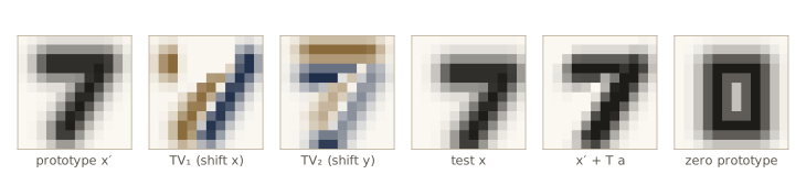
A small experiment makes the comparison systematic: 200 test images, each one of the four shapes shifted by a random amount in both directions plus a little pixel noise, classified by the 1-nearest-neighbor rule over the four prototypes.
rng_td = np.random.default_rng(415)
print("max shift   Euclidean accuracy   tangent accuracy")
for amp in [0.5, 1.0, 1.5, 2.0]:
    hits = np.zeros(2)
    for _ in range(200):
        c = rng_td.integers(4)
        shift = tuple(rng_td.uniform(-amp, amp, 2))
        x = render(SHAPES[NAMES[c]], shift) + 0.05 * rng_td.standard_normal(S_IMG**2)
        d_e = np.linalg.norm(protos - x, axis=1)
        d_t = [tangent_distance(protos[i], tangs[i], x)[0] for i in range(4)]
        hits += [d_e.argmin() == c, np.argmin(d_t) == c]
    print(f"{amp:6.1f}   {hits[0] / 200:14.3f}   {hits[1] / 200:16.3f}")
max shift   Euclidean accuracy   tangent accuracy
   0.5            1.000              1.000
   1.0            0.990              1.000
   1.5            0.945              1.000
   2.0            0.765              0.940
For shifts up to about a stroke width the two agree; as the shifts grow, Euclidean nearest neighbor degrades quickly while tangent distance holds up much longer. Eventually the linear approximation also fails. In real applications (the method was developed for handwritten characters) the tangent vectors cover several transformations at once — both translations, rotation, scaling, shear, and line thickness — and a test pattern is compared with thousands of prototypes. DHS §4.6.2 discusses the construction; the book’s Computer exercises 7 and 8 build a tangent-distance classifier.
Fuzzy classification
Sometimes a designer has informal knowledge instead of data: “a ripe fruit of this kind is yellow and oval.” Fuzzy classification turns such statements into discriminant functions. Each measurable feature is covered by a few overlapping, named ranges — for hue, say, “green”, “yellow-green”, and “yellow”. A membership function \(\mu(x)\) gives, for each range, a number in \([0, 1]\) saying how well the measured value fits the name. To avoid confusion with the classes \(\omega_i\), these named ranges are best called “categories” in quotes: they are properties of one feature, not of the pattern.
A class is then described as a logical combination of “categories”, and a conjunction rule converts the membership values into a discriminant. The most common rule is the product; for a class described as “\(x_1\) is \(A\) and \(x_2\) is \(B\)”,
\[g(\mathbf{x}) = \mu_A(x_1)\,\mu_B(x_2),\]with the obvious extension to more features. The minimum \(\min(\mu_A(x_1), \mu_B(x_2))\) is another popular choice. Both reduce to ordinary logic when the memberships are 0 or 1, and both are symmetric in their arguments, but beyond those two requirements there is little to choose between the many proposed rules. Classification picks the class with the largest discriminant.
The cell encodes two fruit descriptions with triangular membership functions: a “lemon” is yellow and oval, a “lime” is green and round. The features are a hue between 0 (green) and 1 (yellow) and an elongation between 0 (round) and 1 (long).
def tri(x, center, half_width, open_side=None):
    """Triangular membership; open_side 'left' or 'right' makes it 1 beyond the center on that side."""
    m = np.clip(1 - np.abs(x - center) / half_width, 0, 1)
    if open_side == "left":
        m = np.where(x <= center, 1.0, m)
    if open_side == "right":
        m = np.where(x >= center, 1.0, m)
    return m

hue = {"green": lambda v: tri(v, 0.25, 0.45, "left"), "yellow-green": lambda v: tri(v, 0.5, 0.3),
       "yellow": lambda v: tri(v, 0.75, 0.45, "right")}
shape = {"round": lambda v: tri(v, 0.15, 0.45, "left"), "oval": lambda v: tri(v, 0.5, 0.35),
         "long": lambda v: tri(v, 0.85, 0.35, "right")}
classes = {"lemon": ("yellow", "oval"), "lime": ("green", "round")}

fruits = np.array([[0.85, 0.50], [0.15, 0.10], [0.60, 0.30], [0.45, 0.42]])
print("  hue   shape    lemon(prod) lime(prod)   lemon(min) lime(min)")
for h_, e_ in fruits:
    prod = [hue[a](h_) * shape[b](e_) for a, b in classes.values()]
    mins = [min(hue[a](h_), shape[b](e_)) for a, b in classes.values()]
    print(f"  {h_:.2f}  {e_:.2f}   {prod[0]:10.3f} {prod[1]:10.3f}   {mins[0]:10.3f} {mins[1]:9.3f}")
  hue   shape    lemon(prod) lime(prod)   lemon(min) lime(min)
  0.85  0.50        1.000      0.000        1.000     0.000
  0.15  0.10        0.000      1.000        0.000     1.000
  0.60  0.30        0.286      0.148        0.429     0.222
  0.45  0.42        0.257      0.222        0.333     0.400
The two clear cases come out as intended under either rule, and so does the third, a yellowish, slightly round fruit. The last fruit is in between on both features: the product rule calls it a lemon and the minimum rule calls it a lime. Nothing in the designer’s description settles which rule is right — a reminder that the conjunction rule is a design choice with no data behind it.
This resemblance to Parzen windows and PNNs (bumps around typical values, combined by products) invites the question whether memberships are just probabilities. DHS §4.7 takes a clear position. Probability is not only about frequencies of repeatable events; it also quantifies degrees of belief. Cox’s axioms ask only that degrees of belief be ordered like real numbers, that the belief in “not \(a\)” be a function of the belief in \(a\), and that the belief in “\(a\) and \(b\)” be a function of the belief in \(a\) and the belief in \(b\) given \(a\). Any system that satisfies them, scaled to lie between 0 and 1, obeys the rules of probability (DHS Problem 30 outlines the argument). In that view fuzzy memberships add nothing beyond subjective probability.
The practical limitations matter more for a working engineer: fuzzy methods become unwieldy with many features; the designer’s knowledge is limited to the number, positions, and widths of the “categories”; without normalization the discriminants cannot be combined with a changing loss matrix; and pure fuzzy methods do not learn from data. Their real contribution is as a way to turn verbal knowledge into an initial discriminant when there is little or no training data.
Reduced Coulomb energy networks
Parzen windows use one width everywhere; \(k_n\) nearest neighbors adapt the width to the local density. A reduced Coulomb energy (RCE) network takes a third route: it adapts the size of each prototype’s region to the distance to the nearest prototype of a different class. (The name comes from a resemblance between some of its equations and those for the energy of a set of charged particles.)
The network has the same layout as a PNN: input units, one pattern unit per training sample, and category units. Each pattern unit \(j\) stores its prototype \(\mathbf{x}_j\) and a radius \(\lambda_j\), and responds when the input lies inside the sphere \(D(\mathbf{x}, \mathbf{x}_j) < \lambda_j\). (DHS normalizes the patterns so that the distance can be computed by an inner product, as in the PNN; in two dimensions we use Euclidean distances directly.)
Training makes each sphere as large as possible without covering a training point of another class, capped at a maximum radius \(\lambda_m\):
\[\lambda_j = \min\left[\max\left(D(\hat{\mathbf{x}}_j, \mathbf{x}_j),\ \epsilon\right),\ \lambda_m\right], \qquad \hat{\mathbf{x}}_j = \arg\min_{\mathbf{x}\ \text{not in the class of}\ \mathbf{x}_j} D(\mathbf{x}, \mathbf{x}_j),\]where \(\epsilon\) is a small positive floor. Because the sphere is open, the nearest point of another class sits exactly on its surface and is not covered. A unit whose radius comes out very small signals heavily overlapping classes; DHS calls such a unit “probabilistic” and marks it.
Classification collects the spheres containing the test point. If they all belong to one class, that is the answer. If spheres of different classes overlap there, the point is labeled ambiguous; if no sphere contains it, no decision is made. Ambiguous regions are useful information: they show where the classes overlap and where asking a teacher for more labels would help most.
def rce_train(X, y, lam_max, eps=1e-3):
    D = np.sqrt(sq_dists(X, X))
    lam = np.empty(len(X))
    for j in range(len(X)):
        nearest_other = D[j, y != y[j]].min()               # distance to x-hat_j
        lam[j] = min(max(nearest_other, eps), lam_max)
    return lam

def rce_classify(Xq, X, y, lam, c=2):
    """Class label, -1 if no sphere covers x, or -2 if spheres of different classes do."""
    inside = np.sqrt(sq_dists(Xq, X)) < lam[None, :]
    hit = np.stack([(inside & (y == i)[None, :]).any(1) for i in range(c)], axis=1)
    out = np.where(hit.sum(1) == 1, hit.argmax(1), -1)
    out[hit.sum(1) > 1] = -2
    return out

X_rce, y_rce = sample_two_class(30, np.random.default_rng(48))
print("lambda_m   covered & correct   wrong   ambiguous   uncovered   error among decided")
for lam_max in [0.5, 1.0, 2.0]:
    lam = rce_train(X_rce, y_rce, lam_max)
    out = rce_classify(Xt, X_rce, y_rce, lam)
    dec = out >= 0
    print(f"{lam_max:6.1f}   {np.mean(out == yt):14.3f}   {np.mean(dec & (out != yt)):8.3f}"
          f"   {np.mean(out == -2):8.3f}   {np.mean(out == -1):9.3f}   {np.mean(out[dec] != yt[dec]):12.3f}")
lam = rce_train(X_rce, y_rce, 1.0)
print(f"radii with lambda_m = 1.0: min {lam.min():.3f}, median {np.median(lam):.3f}, "
      f"{np.sum(lam == 1.0)} of {len(lam)} at the cap")
err_nn = np.mean(knn_classify(Xt, X_rce, y_rce, 1) != yt)
print(f"1-NN rule on the same 60 prototypes: test error {err_nn:.3f}")
lambda_m   covered & correct   wrong   ambiguous   uncovered   error among decided
   0.5            0.743      0.073      0.041       0.142          0.090
   1.0            0.757      0.058      0.170       0.015          0.071
   2.0            0.748      0.057      0.189       0.007          0.071
radii with lambda_m = 1.0: min 0.004, median 1.000, 34 of 60 at the cap
1-NN rule on the same 60 prototypes: test error 0.133
With a small cap the spheres cover only part of the space, and many test points get no decision; with a large cap almost everything is covered, but the spheres of the two classes overlap more and the ambiguous fraction grows. Among the points that do get a single label, the error is below that of the 1-nearest-neighbor rule on the same 60 points, because the ambiguous points — the hard ones near the boundary — have been set aside. The figure shows the regions.
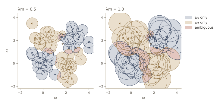
Related methods based on potential functions also place a bump around each prototype and classify by which basins a test point falls into; RCE networks belong to this broader family of relaxation methods. The radius adjustment is what makes RCE training data-driven: each unit covers as much territory as its class can safely claim.
Approximations by series expansions
All the methods of this module store every sample and touch every one of them at classification time. For Parzen windows there is a way out in some cases: expand the window in a series that separates the dependence on \(\mathbf{x}\) from the dependence on the samples. Suppose
\[\varphi\!\left(\frac{\mathbf{x} - \mathbf{x}_i}{h_n}\right) = \sum_{j=1}^{m} a_j\,\psi_j(\mathbf{x})\,\chi_j(\mathbf{x}_i)\]for some functions \(\psi_j\) and \(\chi_j\). Then the sum over samples can be done once, in advance:
\[p_n(\mathbf{x}) = \frac{1}{nV_n}\sum_{i=1}^{n} \varphi\!\left(\frac{\mathbf{x} - \mathbf{x}_i}{h_n}\right) = \sum_{j=1}^{m} b_j\,\psi_j(\mathbf{x}), \qquad b_j = \frac{a_j}{nV_n}\sum_{i=1}^{n} \chi_j(\mathbf{x}_i).\]The \(n\) samples are reduced to \(m\) coefficients, which are easy to update when new samples arrive. If the \(\psi_j\) are polynomials, \(p_n\) is a polynomial, and using \(p_n(\mathbf{x} \mid \omega_i)P(\omega_i)\) as discriminants gives polynomial discriminant functions. Natural choices of expansion include eigenfunctions of the window (viewed as a kernel \(\varphi(\mathbf{x}, \mathbf{x}_i)\), the same object that reappears in Intro to ML, module 06), a least-squares fit with functions orthogonal over the region of interest, or simply a Taylor series.
We take the Taylor series in one dimension, with the Gaussian window written as \(\sqrt{\pi}\,\varphi(u) = e^{-u^2}\). Then
\[e^{-u^{2}} \approx \sum_{j=0}^{m-1} (-1)^{j}\frac{u^{2j}}{j!},\]an alternating series whose error is less than \(u^{2m}/m!\). Substituting \(u = (x - x_i)/h\) gives a polynomial of degree \(2(m-1)\) in \(x\) whose coefficients involve only the power sums \(\sum_i x_i^q\). For \(m = 2\), \(e^{-u^2} \approx 1 - u^2\) and
\[\sqrt{\pi}\,p_n(x) \approx b_0 + b_1 x + b_2 x^{2}, \qquad b_0 = \frac{1}{h} - \frac{1}{h^{3}}\,\frac{1}{n}\sum_{i=1}^{n} x_i^{2}, \quad b_1 = \frac{2}{h^{3}}\,\frac{1}{n}\sum_{i=1}^{n} x_i, \quad b_2 = -\frac{1}{h^{3}}.\]The catch is the one every polynomial has: it grows without bound. The window should fade away from its center, but a truncated series blows up there, so samples far from \(x\) can dominate instead of vanishing. The approximation is only good when every \(\lvert x - x_i \rvert\) is small compared with \(h\). To quantify, let \(r\) be the largest \(\lvert x - x_i \rvert\) that occurs. Each window term then has error below \((r/h)^{2m}/m!\), and with Stirling’s formula \(m! \approx \sqrt{2\pi m}\,(m/e)^m\),
\[\frac{(r/h)^{2m}}{m!} \approx \frac{1}{\sqrt{2\pi m}}\left(\frac{e\,(r/h)^{2}}{m}\right)^{m},\]which becomes small only once \(m > e\,(r/h)^2\). A narrow window needs many terms.
from math import factorial

def taylor_parzen_coeffs(x_samples, h, m):
    """Coefficients b_0..b_{2(m-1)} with sqrt(pi) p_n(x) ~ sum_l b_l x^l (window exp(-u^2)/sqrt(pi))."""
    S = np.array([np.sum(x_samples**q) for q in range(2 * m - 1)])   # power sums: all we keep
    b = np.zeros(2 * m - 1)
    for j in range(m):
        c_j = (-1)**j / (factorial(j) * h**(2 * j))
        for l in range(2 * j + 1):             # (x - x_i)^(2j) = sum_l C(2j, l) x^l (-x_i)^(2j - l)
            b[l] += c_j * comb(2 * j, l) * (-1)**(2 * j - l) * S[2 * j - l]
    return b / (len(x_samples) * h)

x40 = mix_sample(40, np.random.default_rng(416))
h = 2.5
b = taylor_parzen_coeffs(x40, h, 2)
b_formula = [1 / h - np.mean(x40**2) / h**3, 2 * np.mean(x40) / h**3, -1 / h**3]
print("m = 2 coefficients:", np.round(b, 5), " formula:", np.round(b_formula, 5))

xg = np.linspace(-2.5, 3.5, 601)                            # region of interest
r_max = np.max(np.abs(xg[:, None] - x40[None, :]))
for h in [2.5, 1.5]:
    exact = np.exp(-((xg[:, None] - x40[None, :]) / h)**2).sum(1) / (len(x40) * h * np.sqrt(np.pi))
    approx = lambda m: np.polynomial.polynomial.polyval(xg, taylor_parzen_coeffs(x40, h, m)) / np.sqrt(np.pi)
    errs = [np.max(np.abs(approx(m) - exact)) for m in [2, 4, 8, 16, 24, 32, 48]]
    print(f"h = {h}: e(r/h)^2 = {np.e * (r_max / h)**2:5.1f};  max error for m = 2, 4, 8, 16, 24, 32, 48:")
    print("   ", "  ".join(f"{e_:.1e}" for e_ in errs))
m = 2 coefficients: [ 0.2945 -0.0556 -0.064 ]  formula: [ 0.2945 -0.0556 -0.064 ]
h = 2.5: e(r/h)^2 =  15.6;  max error for m = 2, 4, 8, 16, 24, 32, 48:
    4.2e-01  6.5e-01  2.0e-01  3.2e-04  1.2e-08  3.3e-14  8.3e-17
h = 1.5: e(r/h)^2 =  43.2;  max error for m = 2, 4, 8, 16, 24, 32, 48:
    2.5e+00  3.4e+01  7.0e+02  4.6e+03  6.7e+02  6.8e+00  2.6e-06
The \(m = 2\) coefficients match the closed form. With the wide window, the error collapses once \(m\) passes \(e(r/h)^2\), and 40 samples are summarized exactly by a few dozen numbers. With the narrower window the partial sums first grow enormously — the unbounded polynomials at work — and settle only near the predicted number of terms. So the method is attractive only when the window is wide relative to the spread of the data, which is exactly when a Parzen estimate has little resolution. The same tension appears in higher dimensions with more sophisticated expansions.
Summary
| Method | What it assumes | Training | Decision or estimate |
|---|---|---|---|
| Basic estimate \((k/n)/V\) | \(p\) continuous | none | converges if \(V_n \to 0\), \(k_n \to \infty\), \(k_n/n \to 0\) |
| Parzen window | window \(\varphi\) is a bounded density; width \(h_n\) | store samples; choose \(h\) (validation) | \(p_n = \frac{1}{n}\sum_i \delta_n(\mathbf{x} - \mathbf{x}_i)\); bias from blur, variance \(\le \sup\varphi\,\bar{p}_n/(nV_n)\) |
| PNN | normalized patterns, Gaussian window | one pass: \(\mathbf{w}_k = \mathbf{x}_k\) | category sums of \(e^{(\text{net}_k - 1)/\sigma^2}\) = Parzen classifier |
| \(k_n\)-NN density | \(p\) continuous | store samples; choose \(k_n\) | \((k_n/n)/V_n(\mathbf{x})\); adapts to density, not normalizable |
| \(k\)-NN posterior / rule | posteriors continuous | store samples; choose \(k\) | \(P_n(\omega_i \mid \mathbf{x}) = k_i/k\); majority vote |
| 1-NN rule | none | store samples | \(P^* \le P \le P^*(2 - cP^*/(c-1))\) as \(n \to \infty\) |
| Editing / condensing | full training set available | Voronoi, Wilson, or Hart pass | fewer prototypes, same or better decisions |
| Tangent distance | known smooth invariances | tangent vectors per prototype | distance to the prototype’s tangent space |
| Fuzzy classifier | designer’s verbal knowledge | none (hand-designed) | conjunction of membership values |
| RCE network | none | radius = distance to nearest other class, capped | label, ambiguous, or no decision |
| Series expansion | wide window | \(m\) coefficients from power sums | polynomial \(p_n\), accurate if \(m > e(r/h)^2\) |
Ideas to carry forward:
- Every nonparametric estimate trades bias (averaging over a region) against variance (few samples in the region). The theory says how the region must shrink with \(n\); data — through validation or leave-one-out — must choose it for the \(n\) we have.
- The nearest-neighbor rule’s asymptotic error is at most about twice the Bayes error, and voting over \(k\) neighbors approaches the Bayes error. These are large-sample guarantees; in high dimensions they may need impossibly large samples.
- The cost of storing and searching all prototypes is real, and so are the remedies: partial distances, search trees, editing, and condensing.
- The metric carries prior knowledge. Scaling the features, or building in invariances as tangent distance does, often matters more than anything else in a nearest-neighbor classifier. Module 05 turns to the opposite extreme: discriminants with a fixed, simple form whose parameters are learned directly.
Exercises
- For the basic estimate, show that \(\operatorname{Var}[(k/n)/V] = P(1-P)/(nV^2)\). For a region of volume \(V\) around a point where \(p\) is continuous, use \(P \approx p(\mathbf{x})V\) to show that the relative standard deviation is about \(1/\sqrt{np(\mathbf{x})V}\), and explain how this gives the condition \(nV_n \to \infty\).
- Let \(p(x)\) be \(N(\mu, \sigma^2)\) and use a Gaussian window with width \(h\). Show that \(\bar{p}_n(x)\) is the \(N(\mu, \sigma^2 + h^2)\) density and derive the exact variance formula used in the notes. Then find, to leading order in \(h\), the bias at \(x = \mu\), and choose \(h_n\) to minimize the mean squared error there. How does the optimal \(h_n\) scale with \(n\)?
- Show that if the window \(\varphi\) is a density then so is the Parzen estimate \(p_n\), and that the hypercube window gives exactly \((k_n/n)/V_n\). Is the \(k_n\)-nearest-neighbor estimate in one dimension with \(k_n = 2\) integrable? Prove your answer.
- Extend
pnn_classifyto handle unequal known priors \(P(\omega_i)\) that differ from the class fractions. Where in the network do the priors enter? Verify on the three-class data that your network matches a Parzen classifier with those priors. - Prove that every Voronoi cell of the nearest-neighbor rule is convex. Then show that Voronoi editing never changes the decision of the 1-nearest-neighbor rule anywhere in the space.
- Derive the Cover–Hart upper bound for \(c = 2\) directly: show that \(1 - P^2(\omega_1 \mid \mathbf{x}) - P^2(\omega_2 \mid \mathbf{x}) = 2P^*(e \mid \mathbf{x})(1 - P^*(e \mid \mathbf{x}))\), then use the variance argument. Construct a two-class problem in one dimension in which the asymptotic nearest-neighbor error equals \(P^*\) with \(0 < P^* < 1/2\), and check it with
gauss_problem-style grid integration. - Expand \(f_3(p)\) and show that \(f_3(p) = p + 3p^2 - 8p^3 + 4p^4\). Show that \(f_3\) is convex for \(p < (1 - 1/\sqrt{2})/2\), so that its concave majorant \(Q_3\) is a straight line from the origin up to a tangent point and then follows \(f_3\). Find the tangent point and compare with the output of
concave_majorant. - Modify
kd_nearestto return the \(k\) nearest neighbors (keep a heap of the best \(k\) withheapq) and measure how the number of distance computations grows with \(k\) and with \(d\) for uniform data. - Wilson editing uses \(k = 3\). Repeat the editing and condensing experiment for \(k = 1, 3, 7, 15\) and with 500 training points per class, and report the number of kept prototypes and the test error. Which combination comes closest to the Bayes error with the fewest prototypes?
- Add a rotation tangent vector to
translation_tangents(rotate the strokes about the image center by a small angle), add rotated test images to the experiment, and compare Euclidean distance, tangent distance with translations only, and tangent distance with translations and rotation. - For the RCE network, show that if no two training points of different classes are closer than \(\epsilon\), the trained network classifies every training point correctly. Then modify
rce_classifyto fall back to the nearest-neighbor rule for uncovered points, and compare its error with that of the plain 1-NN rule on the same 60 points. - In your own words: why is it remarkable that, with unlimited data, a rule that looks only at the single nearest neighbor has at most about twice the Bayes error, and why does this result offer little comfort when the features have fifty dimensions?
Going further
- R. O. Duda, P. E. Hart, and D. G. Stork, Pattern Classification, 2nd ed., chapter 4. Problems 1–4 (Parzen convergence and bias), 5–6 (\(k_n\)-nearest-neighbor estimates), 7–18 (the nearest-neighbor rule, editing, the zero-information case, and the \(k\)-NN bound), 19–27 (metrics and tangent distance), 28–30 (fuzzy methods and Cox’s axioms), 31 (RCE), and 32 onward (series expansions) extend the sections above; Computer exercises 1–11 follow the same sections in order.
- E. Parzen, “On estimation of a probability density function and mode”, The Annals of Mathematical Statistics, 1962 — the window method and its convergence theory.
- T. M. Cover and P. E. Hart, “Nearest neighbor pattern classification”, IEEE Transactions on Information Theory, 1967 — the asymptotic bounds proved in this module.
- P. E. Hart, “The condensed nearest neighbor rule”, IEEE Transactions on Information Theory, 1968, and D. L. Wilson, “Asymptotic properties of nearest neighbor rules using edited data”, IEEE Transactions on Systems, Man, and Cybernetics, 1972 — condensing and editing.
- D. F. Specht, “Probabilistic neural networks”, Neural Networks, 1990; and P. Y. Simard, Y. LeCun, and J. S. Denker, “Efficient pattern recognition using a new transformation distance”, Advances in Neural Information Processing Systems 5, 1993 — the PNN and tangent distance.
- In the Intro to ML notes: kernel density estimation, nearest-neighbor density estimates, and the \(K\)-nearest-neighbor classifier in Intro to ML, module 02, and kernels as similarity functions in Intro to ML, module 06.
These notes follow the chapters of R. O. Duda, P. E. Hart, and D. G. Stork, Pattern Classification, 2nd edition (Wiley, 2001), the course text. The explanations, code, figures, and exercises here are written for this course; the book remains the reference, with the full derivations, worked examples, and many more problems.