CSE 455/555 · Module 08 · Session 8
Nonmetric Methods: Trees, Strings, and Grammars
Classification without a distance — decision trees (CART, ID3, C4.5) with impurity, stopping, pruning, and missing attributes; string matching and edit distance; grammars, parsing, and grammatical inference; and learning if–then rules.
Companion reading: Duda, Hart & Stork, Pattern Classification, chapter 8, “Nonmetric Methods”
By the end of this module you can
- Grow a binary decision tree with entropy or Gini impurity, explain why any multiway tree can be made binary, and show with a concrete split why misclassification impurity is a poor splitting criterion.
- Implement CART for numeric features from scratch, stop its growth with impurity thresholds, a chi-squared test, or a description-length criterion, and prune it by cost-complexity pruning with a validation set.
- Explain the horizon effect, the instability of greedy trees, and why oblique (multivariate) splits can replace dozens of axis-parallel ones.
- Build trees that respect priors and misclassification costs, and classify patterns with missing attributes using surrogate splits or C4.5’s weighted descent.
- Compare ID3, C4.5, and CART, and show why information gain favors many-valued attributes and how the gain ratio corrects it.
- Match strings with the naive and Boyer–Moore algorithms, compute edit distance and an optimal alignment by dynamic programming, and extend it to matching with errors and with a don’t-care symbol.
- Define a grammar, place it in the Chomsky hierarchy, and decide membership of a string with the CYK parser for a grammar in Chomsky normal form.
- Describe grammatical inference from positive and negative examples, and learn a set of if–then rules by sequential covering.
Contents
- Nominal data and nonmetric patterns
- Decision trees
- CART
- Number of splits
- Query selection and node impurity
- Why misclassification impurity is a poor splitting criterion
- The twoing criterion
- Implementing CART for numeric features
- A two-dimensional test problem
- When to stop splitting
- Pruning
- Assigning leaf labels
- Instability
- Computational complexity
- Feature choice
- Multivariate decision trees
- Priors and costs
- Missing attributes
- Other tree methods
- Recognition with strings
- Grammatical methods
- Grammatical inference
- Rule-based methods
- Summary
- Exercises
- Going further
Every classifier so far has leaned on numbers. Bayes rules in module 02 needed densities over a real feature space; the nearest-neighbor rules of module 04 needed a distance; the linear machines of module 05 and the networks of module 06 needed inner products and gradients. This module drops that assumption. Its patterns are lists of attributes such as “soil = sandy, light = bright”, or strings of symbols such as a DNA fragment or a sequence of pen strokes, and there is no natural way to say how far apart two of them are.
Duda, Hart & Stork (DHS) collect three families of methods for such data in chapter 8, and we follow their order. Decision trees classify by asking a sequence of questions, each of which needs only a yes or a no; they are the largest part of the module, because they are also among the most useful classifiers for ordinary numeric data. String methods find a pattern inside a long text, measure how many edits turn one string into another, and so turn nearest-neighbor classification loose on sequences. Grammatical methods assume the strings were produced by rewrite rules, recognize a string by parsing it, and try to learn the rules from examples. A short final section learns if–then rules directly.
Nothing here needs heavy mathematics. What it needs is care with combinatorial search: most of the algorithms are greedy or dynamic-programming procedures, and we implement each of them from scratch and check it against brute force on small cases. Trees return in module 09, where resampling and combining classifiers make up for their instability; the ML notes treat trees as components of committees and mixtures in Intro to ML, module 14.
The first cell loads the tools the whole module uses.
import numpy as np
import copy, itertools
from collections import Counter
from scipy.special import erfc

np.set_printoptions(precision=4, suppress=True)
rng = np.random.default_rng(808)
Nominal data and nonmetric patterns
A nominal attribute takes values from a finite set with no order and no distance: the color of a fruit, a blood type, the suit of a card. Two common ways to describe a pattern with such values are:
- a property \(d\)-tuple, a fixed list of \(d\) attribute values, for example (light = bright, water = weekly, pot = clay, humidity = dry);
- a string, a variable-length sequence of symbols from a finite alphabet, for example the base sequence “GATTACA” or a chain of stroke types produced by an earlier classifier.
Why not code the values as numbers and use the old methods? We can, and sometimes it works, but any coding invents structure. If we write low, medium, bright as 0, 1, 2, a linear machine will assume that medium lies halfway between the other two, which may be harmless for light levels; if we code the pot materials clay, plastic, glass as 0, 1, 2, the same machine will “learn” from an ordering that does not exist. The methods of this module use only tests of equality and set membership, so they never need such a coding. DHS keep bold symbols such as \(\mathbf{x}\) for these patterns even though they cannot be added or scaled; we do the same, and follow their habit of saying attribute for a value of any kind and feature for a real-valued one.
Decision trees
A natural way to classify with nominal data is to play twenty questions: ask about one attribute, and let the answer decide what to ask next. A decision tree records such a questioning strategy. The first question sits at the root node, drawn at the top. Each possible answer is a link (or branch) to a descendent node, which asks the next question. A node with no outgoing links is a leaf and carries a category label. Any node together with everything below it is a subtree. The links leaving a node must be mutually exclusive and exhaustive, so that every pattern follows exactly one path from the root to a leaf, and the pattern is assigned the leaf’s label.
Our running nominal example is a small houseplant problem. Each plant is described by four attributes — light (low, medium, bright), water (sparse, weekly, daily), pot (clay, plastic), and humidity (dry, humid) — and the categories are \(\omega_1\) = thrives and \(\omega_2\) = struggles. The cell stores a tree for this problem as nested dictionaries: an internal node names its attribute and maps each value to a subtree, and a leaf is just a label.
ATTRS = {"light": ["low", "medium", "bright"], "water": ["sparse", "weekly", "daily"],
         "pot": ["clay", "plastic"], "humidity": ["dry", "humid"]}

plant_tree = {"attr": "water", "branches": {
    "sparse": "struggles",
    "weekly": {"attr": "light", "branches": {"low": "struggles", "medium": "thrives",
                                             "bright": "thrives"} },
    "daily":  {"attr": "humidity", "branches": {
        "dry": "struggles",
        "humid": {"attr": "light", "branches": {"low": "struggles", "medium": "struggles",
                                                "bright": "thrives"} } } } } }

def classify_nominal(tree, x):
    """Follow one path from the root to a leaf; x is a dict attribute -> value."""
    while isinstance(tree, dict):
        tree = tree["branches"][x[tree["attr"]]]
    return tree

def tree_rules(tree, path=()):
    """One conjunction (list of attribute = value tests) per leaf."""
    if not isinstance(tree, dict):
        return [(path, tree)]
    out = []
    for v, sub in tree["branches"].items():
        out += tree_rules(sub, path + ((tree["attr"], v),))
    return out

x = {"light": "bright", "water": "daily", "pot": "clay", "humidity": "humid"}
print("classified as:", classify_nominal(plant_tree, x))
for conds, label in tree_rules(plant_tree):
    if label == "thrives":
        print("thrives IF", " AND ".join(a + "=" + v for a, v in conds))
classified as: thrives
thrives IF water=weekly AND light=medium
thrives IF water=weekly AND light=bright
thrives IF water=daily AND humidity=humid AND light=bright
The printout shows the main attraction of trees, interpretability. The decision for any single pattern is the conjunction of the tests on its path, and a whole category is the disjunction (OR) of the paths that end in its leaves. Here “thrives” is the union of three conjunctions, which a person can read, check against expert knowledge, and simplify: the first two rules merge into (water = weekly AND light \(\neq\) low). Trees are also fast at classification time, since a pattern answers only the questions on one path, and they give an easy place to insert prior knowledge from a domain expert, which helps most when the problem is simple and training data are scarce.
CART
Now suppose we have a labeled training set \(\mathcal{D}\) and a list of attributes, but no tree. Every tree splits \(\mathcal{D}\) into smaller and smaller subsets as we move down from the root. If all the samples in a subset carry the same label, the subset is pure, and that branch can end in a leaf. Otherwise we must decide whether to accept an imperfect leaf or to ask another question. This suggests a recursive procedure: at a node, either declare it a leaf with some label, or choose a question, split the data, and repeat on each part.
CART (classification and regression trees) is the general framework built around this recursion. To use it we must answer six design questions, and the subsections below take them in turn:
- How many outcomes (splits) should a question have — two, or more?
- Which question should a node ask?
- When should a node become a leaf?
- If the tree grows too large, how should it be pruned back?
- If a leaf is impure, which label should it carry?
- How should missing attribute values be handled?
Number of splits
The number of links leaving a node is its branching factor \(B\). The houseplant tree has \(B = 3\) at its water node and \(B = 2\) at its humidity node. Nothing forces a single \(B\) throughout, but we never need more than two: a node with \(B\) outcomes \(v_1, \dots, v_B\) can be replaced by a chain of \(B - 1\) binary nodes asking “is the value \(v_1\)?”, then (on the no branch) “is it \(v_2\)?”, and so on. Applied recursively this turns any tree into a binary tree that implements the same classifier. The cell does exactly that and checks the claim on all \(3 \cdot 3 \cdot 2 \cdot 2 = 36\) possible plants.
def to_binary(tree):
    """Replace every B-way node by a chain of B-1 yes/no questions (yes = left)."""
    if not isinstance(tree, dict):
        return tree
    items = list(tree["branches"].items())
    node = to_binary(items[-1][1])                 # the last value needs no question
    for v, sub in reversed(items[:-1]):
        node = {"test": (tree["attr"], v), "yes": to_binary(sub), "no": node}
    return node

def classify_binary(tree, x):
    while isinstance(tree, dict):
        a, v = tree["test"]
        tree = tree["yes"] if x[a] == v else tree["no"]
    return tree

def count_nodes(tree):
    if not isinstance(tree, dict):
        return 0
    kids = tree["branches"].values() if "branches" in tree else (tree["yes"], tree["no"])
    return 1 + sum(count_nodes(k) for k in kids)

all_plants = [dict(zip(ATTRS, vals)) for vals in itertools.product(*ATTRS.values())]
bin_tree = to_binary(plant_tree)
same = all(classify_binary(bin_tree, p) == classify_nominal(plant_tree, p)
           for p in all_plants)
print(f"{len(all_plants)} plants, identical decisions: {same}")
print(f"question nodes: multiway {count_nodes(plant_tree)}, "
      f"binary {count_nodes(bin_tree)}")
36 plants, identical decisions: True
question nodes: multiway 4, binary 7
The binary tree asks more, simpler questions and implements the same function. Because every tree has a binary equivalent, and because choosing a single yes/no question is a much easier search than choosing a \(B\)-way partition, we concentrate on binary trees; by convention the yes branch goes to the left.
For real-valued features the most common question is “is \(x_i < x_{is}\)?” for one feature \(x_i\) and a threshold \(x_{is}\). A tree built only from such questions is monothetic (each question uses one attribute); its decision boundary is made of pieces of hyperplanes perpendicular to the coordinate axes, so the decision regions are unions of axis-aligned boxes. A tree whose questions combine several attributes, such as \(\mathbf{w}^{t}\mathbf{x} < w_0\) or (size = small AND color \(\neq\) red), is polythetic. With enough boxes a monothetic tree can approximate any boundary, but, as we will see, it may need a great many of them.
Query selection and node impurity
Which question should a node ask? The guiding principle is simplicity, a form of Occam’s razor: prefer questions that lead to a small tree. Greedily, that means choosing the question that makes the data reaching the two children as pure as possible. It is more convenient to measure the opposite, the impurity \(i(N)\) of a node \(N\), which should be 0 when all samples at \(N\) share one category and largest when all categories are equally represented. Write \(P(\omega_j)\) for the fraction of the samples at \(N\) that belong to \(\omega_j\) (strictly a sample frequency at that node, not a prior; DHS use the same shorthand). Three impurities are in common use.
The entropy impurity (also called information impurity) is
\[i(N) = -\sum_{j=1}^{c} P(\omega_j)\log_2 P(\omega_j),\]with \(0 \log_2 0 = 0\). It is the average number of bits needed to code the label of a sample drawn at \(N\); it is 0 for a pure node and \(\log_2 c\) when the \(c\) categories are equally frequent.
The Gini impurity is
\[i(N) = \sum_{i \neq j} P(\omega_i)P(\omega_j) = 1 - \sum_{j=1}^{c} P^2(\omega_j).\]It is the error rate we would get at \(N\) by drawing the label at random from the node’s own class frequencies. With two categories it becomes \(2P(\omega_1)P(\omega_2)\); the product \(P(\omega_1)P(\omega_2)\) alone is called the variance impurity, because it is the variance of a variable that equals 1 for \(\omega_1\) and 0 for \(\omega_2\).
The misclassification impurity is
\[i(N) = 1 - \max_j P(\omega_j),\]the training error at \(N\) if we label it with its majority category. It is the most sharply peaked of the three, and its derivative jumps where the majority changes.
When a question \(s\) sends a fraction \(P_L\) of the samples at \(N\) to the left child \(N_L\) and the rest to \(N_R\), the drop in impurity is
\[\Delta i(s) = i(N) - P_L\, i(N_L) - (1 - P_L)\, i(N_R),\]and the greedy rule picks the \(s\) that maximizes it. Because only the location of the maximum matters, adding a constant to \(i\) or scaling it by a positive factor changes nothing. With entropy impurity, \(\Delta i\) is the information gain of the question: the mutual information between the category and the answer. Since a yes/no answer carries at most one bit, a binary split can never reduce entropy impurity by more than one bit, whatever the number of categories. (Formally, mutual information is bounded by the entropy of either variable, and the answer’s entropy is at most \(\log_2 2 = 1\).)
The cell implements the three impurities so that they work on a whole array of probability vectors at once (the class index is the last axis), which the split search below relies on.
def entropy_imp(P):
    P = np.asarray(P, float)
    logs = np.log2(np.where(P > 0, P, 1.0))      # 0 log 0 = 0
    return 0.0 - (P * logs).sum(axis=-1)

def gini_imp(P):
    P = np.asarray(P, float)
    return 1.0 - (P ** 2).sum(axis=-1)

def misclass_imp(P):
    P = np.asarray(P, float)
    return 1.0 - P.max(axis=-1)

IMPURITIES = {"entropy": entropy_imp, "gini": gini_imp, "misclass": misclass_imp}
for P in ([1.0, 0.0, 0.0], [0.5, 0.5, 0.0], [1/3, 1/3, 1/3], [0.7, 0.2, 0.1]):
    vals = "  ".join(f"{k} {f(P):.4f}" for k, f in IMPURITIES.items())
    print(f"P = {np.round(P, 3)}  ->  {vals}")
P = [1. 0. 0.]  ->  entropy 0.0000  gini 0.0000  misclass 0.0000
P = [0.5 0.5 0. ]  ->  entropy 1.0000  gini 0.5000  misclass 0.5000
P = [0.333 0.333 0.333]  ->  entropy 1.5850  gini 0.6667  misclass 0.6667
P = [0.7 0.2 0.1]  ->  entropy 1.1568  gini 0.4600  misclass 0.3000
All three vanish on a pure node and peak at the uniform distribution, where entropy reaches \(\log_2 3 = 1.585\) bits and Gini reaches \(1 - 1/3\).
Why misclassification impurity is a poor splitting criterion
The three impurities usually agree on which split is best, but the misclassification impurity has a blind spot. Take a node with 60 samples of \(\omega_1\) and 15 of \(\omega_2\), and a question that sends 25 of the \(\omega_1\) samples, and nothing else, to the left:
| \(\omega_1\) | \(\omega_2\) | \(P(\omega_2)\) | |
|---|---|---|---|
| parent \(N\) | 60 | 15 | 0.2 |
| left child \(N_L\) | 25 | 0 | 0 |
| right child \(N_R\) | 35 | 15 | 0.3 |
This is a useful split: a third of the data is now settled, and the \(\omega_2\) samples are concentrated on the right, where a later question can go after them. Yet both children still have \(\omega_1\) as their majority, so the misclassification impurity says nothing has improved.
def impurity_drop(parent, left, right, imp):
    parent, left, right = (np.asarray(v, float) for v in (parent, left, right))
    P_L = left.sum() / parent.sum()
    return (imp(parent / parent.sum()) - P_L * imp(left / left.sum())
            - (1 - P_L) * imp(right / right.sum()))

for name, f in IMPURITIES.items():
    d = impurity_drop([60, 15], [25, 0], [35, 15], f)
    print(f"{name:9s} drop = {np.round(d, 12) + 0.0:.4f}")     # round away float noise
entropy   drop = 0.1344
gini      drop = 0.0400
misclass  drop = 0.0000
The reason is geometric. With two categories each impurity is a function of \(p = P(\omega_2)\), and the parent’s \(p\) is the \(P_L\)-weighted average of the children’s: \(0.2 = \tfrac{1}{3}\cdot 0 + \tfrac{2}{3}\cdot 0.3\). The weighted child impurity \(P_L i(N_L) + (1 - P_L) i(N_R)\) is therefore the height, above the parent’s \(p\), of the chord joining the two children’s points on the impurity curve, and \(\Delta i\) is the gap between the curve and that chord. For a strictly concave impurity such as entropy or Gini, the chord lies strictly below the curve unless the children have identical class frequencies, so every split that separates the classes at all earns a positive drop. The misclassification impurity is concave but piecewise linear: on each side of \(p = 0.5\) it is a straight line, and whenever both children fall on the same side, the chord lies on the curve and the drop is exactly zero.
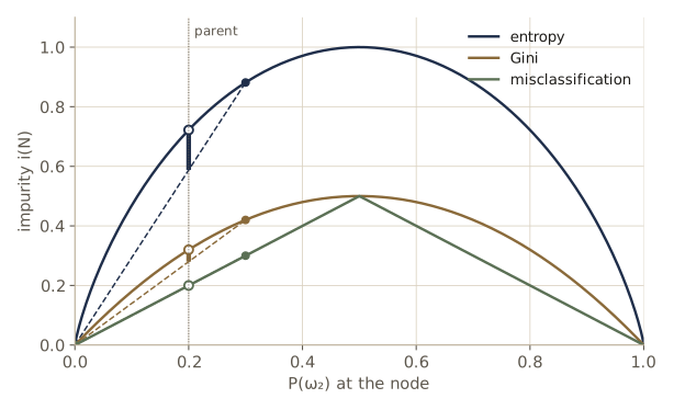
The blind spot matters in practice when no single question can create a node where the minority class wins. The next cell builds such a data set: a regular grid on the unit square whose upper-right corner, \(x_1 > 0.6\) and \(x_2 > 0.6\), belongs to \(\omega_2\). Any single threshold leaves \(\omega_1\) in the majority on both sides, so the misclassification drop is zero for every candidate question and a tree grown with it never leaves the root. (The split search best_split used here is defined in the next subsection; the runner executes the cells in order, so we show this experiment’s result after it.)
Watch out. Misclassification rate is the quantity we finally care about, which makes it tempting to split on it. Resist: an impurity that is strictly concave “anticipates” later useful splits, while the misclassification impurity sees only immediate changes of majority. It remains a reasonable criterion for pruning, where we compare whole subtrees rather than single steps.
The twoing criterion
With many categories, DHS describe a strategic variant called the twoing criterion. At each node we consider every way of grouping the \(c\) categories into two supercategories \(C_1\) and \(C_2 = \{\omega_1, \dots, \omega_c\} \setminus C_1\), treat the node as a two-class problem between \(C_1\) and \(C_2\), find the best split for that problem, and finally keep the grouping and split with the largest drop. The idea is that the first questions should separate large groups of similar categories, leaving fine distinctions for deeper nodes.
With the Gini impurity the search over groupings has a closed form. For a fixed split, let \(q_L\) and \(q_R\) be the fractions of the left and right samples that belong to \(C_1\), so that the parent’s fraction is \(q = P_L q_L + P_R q_R\) with \(P_R = 1 - P_L\). A short calculation with \(i = 2q(1-q)\) gives
\[\Delta i = 2q(1-q) - 2P_L q_L(1-q_L) - 2P_R q_R(1-q_R) = 2P_LP_R\,(q_L - q_R)^2 .\]Now \(q_L - q_R = \sum_{j \in C_1}\left[P(\omega_j \mid N_L) - P(\omega_j \mid N_R)\right]\), and the bracketed differences sum to zero over all \(j\). The absolute value of such a partial sum is largest when \(C_1\) collects exactly the categories with a positive difference, and then it equals half the sum of the absolute differences. So the best grouping for a given split achieves
Result. For two-class Gini impurity, the twoing value of a split is
\[\max_{C_1} \Delta i = \frac{P_L P_R}{2}\left(\sum_{j=1}^{c} \left\lvert P(\omega_j \mid N_L) - P(\omega_j \mid N_R) \right\rvert\right)^2 ,\]attained by putting in \(C_1\) every category that is more frequent on the left than on the right.
This is the form in which the criterion is usually quoted (up to a constant factor, which does not matter). The cell checks it against brute force over all \(2^{c-1} - 1\) groupings for a split of five categories.
def twoing_bruteforce(nL, nR, imp=gini_imp):
    """Largest two-class impurity drop over all groupings C1 / C2 of the categories."""
    c, best = len(nL), (-1.0, None)
    for r in range(1, c):
        for C1 in itertools.combinations(range(c), r):
            if 0 not in C1:              # count each grouping once: C1 holds category 0
                continue
            m = np.isin(np.arange(c), C1)
            two = lambda v: [v[m].sum(), v[~m].sum()]
            d = impurity_drop(two(nL + nR), two(nL), two(nR), imp)
            best = max(best, (d, C1))
    return best

def twoing_gini(nL, nR):
    PL = nL.sum() / (nL.sum() + nR.sum())
    diff = nL / nL.sum() - nR / nR.sum()
    return PL * (1 - PL) / 2 * np.abs(diff).sum() ** 2

nL = np.array([30.0, 4.0, 18.0, 2.0, 12.0])     # counts of the 5 categories sent left
nR = np.array([5.0, 20.0, 16.0, 25.0, 9.0])     # ... and sent right
d_bf, C1 = twoing_bruteforce(nL, nR)
print("left counts", nL, " right counts", nR)
print(f"brute force {d_bf:.6f} with C1 = {C1};  closed form {twoing_gini(nL, nR):.6f}")
print("categories more frequent on the left:",
      [int(j) for j in np.flatnonzero(nL / nL.sum() > nR / nR.sum())])
left counts [30.  4. 18.  2. 12.]  right counts [ 5. 20. 16. 25.  9.]
brute force 0.129059 with C1 = (0, 2, 4);  closed form 0.129059
categories more frequent on the left: [0, 2, 4]
The search over all fifteen groupings lands on exactly the categories that are relatively more frequent on the left (code indices 0, 2, 4, that is \(\omega_1, \omega_3, \omega_5\)), and the closed form matches. In general the search may report the complement instead, since a grouping and its complement describe the same two-class problem.
How much does the choice of impurity matter overall? Less than one might expect. In practice the resulting trees and their accuracies are usually similar; entropy is a common default, Gini is CART’s traditional choice, and the decisions about when to stop and how to prune matter far more.
Implementing CART for numeric features
We now have enough to grow a tree. For numeric features the candidate questions at a node are “is \(x_i < x_{is}\)?” for every feature \(i\) and every threshold \(x_{is}\). Only thresholds between consecutive distinct values of \(x_i\) among the node’s samples give different splits, so with \(n\) samples there are at most \(n - 1\) candidates per feature; within each gap the drop in impurity is constant, and we follow the common habit of placing the threshold at the midpoint. Sorting the samples on \(x_i\) lets us compute the class counts to the left of every candidate at once with a cumulative sum, and the vectorized impurities then give all the drops in one line.
The tree itself is a dictionary per node. Every node stores its class counts counts and its majority label; an internal node also stores the feature feat, the threshold thr, and the subtrees left (the yes answer, \(x_i < x_{is}\)) and right. Class labels in code are the integers \(0, \dots, c-1\) for \(\omega_1, \dots, \omega_c\). Optional sample weights w will be used later for priors and costs; without them every sample counts once.
def best_split(X, y, c, impurity, w=None):
    """Best single-feature question 'x_j < thr?' by drop in impurity: (drop, j, thr)."""
    n, d = X.shape
    w = np.ones(n) if w is None else w
    Y = np.eye(c)[y] * w[:, None]                # weighted one-hot labels
    total = Y.sum(axis=0)
    i_parent = impurity(total / total.sum())
    best = (0.0, None, None)
    for j in range(d):
        order = np.argsort(X[:, j], kind="stable")
        xs = X[order, j]
        CL = np.cumsum(Y[order], axis=0)[:-1]   # class totals left of each gap
        CR = total - CL
        ok = xs[1:] > xs[:-1]                   # only gaps between distinct values
        if not ok.any():
            continue
        CL, CR = CL[ok], CR[ok]
        P_L = CL.sum(axis=1) / total.sum()
        drop = (i_parent - P_L * impurity(CL / CL.sum(axis=1, keepdims=True))
                - (1 - P_L) * impurity(CR / CR.sum(axis=1, keepdims=True)))
        k = np.argmax(drop)
        if drop[k] > best[0] + 1e-12:
            thr = 0.5 * (xs[1:][ok][k] + xs[:-1][ok][k])      # midpoint of the gap
            best = (float(drop[k]), j, float(thr))
    return best

def grow(X, y, c, impurity=gini_imp, min_gain=0.0, min_leaf=1, max_depth=50,
         split_ok=None, w=None, depth=0):
    """Recursive CART growth. Stops at pure nodes, or when a stopping rule fires."""
    wv = np.ones(len(y)) if w is None else w
    counts = np.bincount(y, weights=wv, minlength=c)
    node = {"counts": counts, "label": int(np.argmax(counts)), "depth": depth}
    if np.count_nonzero(counts) <= 1 or depth >= max_depth or len(y) < 2 * min_leaf:
        return node
    gain, j, thr = best_split(X, y, c, impurity, w)
    if j is None or gain <= min_gain:
        return node
    go = X[:, j] < thr
    if min(go.sum(), (~go).sum()) < min_leaf:
        return node
    nL = np.bincount(y[go], weights=wv[go], minlength=c)
    if split_ok is not None and not split_ok(counts, nL, counts - nL, gain):
        return node
    kw = dict(impurity=impurity, min_gain=min_gain, min_leaf=min_leaf,
              max_depth=max_depth, split_ok=split_ok, depth=depth + 1)
    node.update(feat=j, thr=thr, gain=gain,
                left=grow(X[go], y[go], c, w=None if w is None else w[go], **kw),
                right=grow(X[~go], y[~go], c, w=None if w is None else w[~go], **kw))
    return node

def is_leaf(t):
    return "feat" not in t

def n_leaves(t):
    return 1 if is_leaf(t) else n_leaves(t["left"]) + n_leaves(t["right"])

def predict(t, X):
    """Send all rows of X down the tree at once, splitting index sets at each node."""
    out = np.empty(len(X), dtype=int)
    def route(t, idx):
        if is_leaf(t):
            out[idx] = t["label"]
            return
        m = X[idx, t["feat"]] < t["thr"]
        route(t["left"], idx[m])
        route(t["right"], idx[~m])
    route(t, np.arange(len(X)))
    return out

def show_tree(t, names=("x1", "x2"), indent=""):
    if is_leaf(t):
        return f"{indent}-> w{t['label'] + 1}  counts {t['counts'].astype(int)}\n"
    q = f"{names[t['feat']]} < {t['thr']:.3f} ?"
    s = f"{indent}{q}   counts {t['counts'].astype(int)}\n"
    deeper = indent + "    "
    return s + show_tree(t["left"], names, deeper) + show_tree(t["right"], names, deeper)

def error_rate(t, X, y):
    return float(np.mean(predict(t, X) != y))
A first test on a small data set we can check by hand: ten readings of two features for a pump, vibration \(x_1\) and temperature \(x_2\) (arbitrary units), with \(\omega_1\) = normal and \(\omega_2\) = worn. Before trusting the vectorized search we compare its root split with a slow loop that tries every midpoint of every feature and evaluates the drop directly from the definition.
X_pump = np.array([[1.0, 4.2], [1.6, 3.1], [2.2, 4.8], [2.9, 3.9], [3.1, 2.2],
                   [3.8, 4.4], [4.5, 3.6], [5.1, 1.8], [5.7, 4.9], [2.4, 1.3]])
y_pump = np.array([0, 0, 0, 0, 0, 1, 1, 1, 1, 1])

def best_split_slow(X, y, c, impurity):
    best = (0.0, None, None)
    for j in range(X.shape[1]):
        v = np.unique(X[:, j])
        for thr in (v[1:] + v[:-1]) / 2:
            m = X[:, j] < thr
            d = impurity_drop(np.bincount(y, minlength=c), np.bincount(y[m], minlength=c),
                              np.bincount(y[~m], minlength=c), impurity)
            if d > best[0] + 1e-12:
                best = (d, j, thr)
    return best

for name in ("entropy", "gini"):
    f = IMPURITIES[name]
    fast, slow = best_split(X_pump, y_pump, 2, f), best_split_slow(X_pump, y_pump, 2, f)
    print(f"{name:8s} fast: drop {fast[0]:.4f} on x{fast[1] + 1} < {fast[2]:.2f}   "
          f"slow: drop {slow[0]:.4f} on x{slow[1] + 1} < {slow[2]:.2f}")

pump_tree = grow(X_pump, y_pump, 2, entropy_imp)
print(show_tree(pump_tree))
print(f"training error {error_rate(pump_tree, X_pump, y_pump):.2f}")
entropy  fast: drop 0.6100 on x1 < 3.45   slow: drop 0.6100 on x1 < 3.45
gini     fast: drop 0.3333 on x1 < 3.45   slow: drop 0.3333 on x1 < 3.45
x1 < 3.450 ?   counts [5 5]
    x2 < 1.750 ?   counts [5 1]
        -> w2  counts [0 1]
        -> w1  counts [5 0]
    -> w2  counts [0 4]

training error 0.00
Both searches agree. The grown tree first separates the worn pumps with high vibration, then catches the single worn pump with low vibration by its low temperature. Every leaf is pure, so the training error is zero.
Now the experiment promised in the previous subsection: a regular \(20 \times 20\) grid whose upper-right corner is \(\omega_2\).
g = (np.arange(20) + 0.5) / 20
X_grid = np.array([(a, b) for a in g for b in g])
y_grid = ((X_grid[:, 0] > 0.6) & (X_grid[:, 1] > 0.6)).astype(int)

for name in ("misclass", "gini", "entropy"):
    t = grow(X_grid, y_grid, 2, IMPURITIES[name])
    print(f"{name:9s} leaves {n_leaves(t)}   training error "
          f"{error_rate(t, X_grid, y_grid):.3f}")
print(show_tree(grow(X_grid, y_grid, 2, gini_imp)))
misclass  leaves 1   training error 0.160
gini      leaves 3   training error 0.000
entropy   leaves 3   training error 0.000
x1 < 0.600 ?   counts [336  64]
    -> w1  counts [240   0]
    x2 < 0.600 ?   counts [96 64]
        -> w1  counts [96  0]
        -> w2  counts [ 0 64]
With the misclassification impurity every candidate drop is zero, so the tree stays a single leaf that calls everything \(\omega_1\) and misclassifies the 16% of the grid in the corner. Gini and entropy take the useful first step that does not change any majority, and the second question then isolates the corner exactly.
A two-dimensional test problem
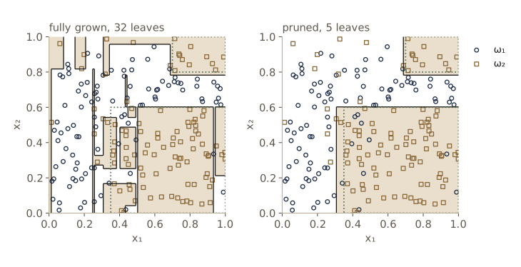
For the rest of the tree sections we use a synthetic two-category problem on the unit square. The category is \(\omega_2\) inside two axis-aligned boxes, \(\{x_1 > 0.35,\ x_2 < 0.6\}\) and \(\{x_1 > 0.7,\ x_2 > 0.8\}\), and \(\omega_1\) elsewhere; then 10% of the labels are flipped at random, so the Bayes error is 10%. We draw 200 training points, 200 validation points (for choosing how far to prune), and 5000 test points (for measuring the result). A fully grown tree fits the training data exactly.
def make_boxes(n, gen, flip=0.10):
    X = gen.random((n, 2))
    inside = ((X[:, 0] > 0.35) & (X[:, 1] < 0.6)) | ((X[:, 0] > 0.7) & (X[:, 1] > 0.8))
    y = inside.astype(int)
    noisy = gen.random(n) < flip
    return X, np.where(noisy, 1 - y, y)

gen = np.random.default_rng(8)
X_tr, y_tr = make_boxes(200, gen)
X_va, y_va = make_boxes(200, gen)
X_te, y_te = make_boxes(5000, gen)

full_tree = grow(X_tr, y_tr, 2, gini_imp)
print(f"fully grown: {n_leaves(full_tree)} leaves   "
      f"train error {error_rate(full_tree, X_tr, y_tr):.3f}   "
      f"test error {error_rate(full_tree, X_te, y_te):.3f}")
fully grown: 32 leaves train error 0.000 test error 0.215
A training error of zero with a test error roughly twice the Bayes rate is the signature of overfitting: many of the leaves exist only to isolate a single flipped label. The next two subsections are about avoiding that.
When to stop splitting
If we split until every leaf is pure, the tree becomes a lookup table for the training set and generalizes poorly whenever the classes overlap. If we stop too early, the training error stays high and so does the test error. There are several ways to decide when a node should stop.
Validation. Hold out part of the data, grow the tree on the rest, and stop growing (for example, stop adding levels) when the error on the held-out part stops falling. Cross-validation repeats this over several splits of the data (module 09). The cost is that the held-out samples are not used to grow the tree.
A threshold on the impurity drop. Stop at a node if the best split reduces impurity by less than some \(\beta\), that is, if \(\max_s \Delta i(s) \le \beta\). This uses all the data, and leaves can end up at different depths, which suits problems whose complexity varies across feature space. The difficulty is that there is rarely a simple relation between \(\beta\) and the final accuracy.
A threshold on node size. Stop when a node holds fewer than some number of samples, or some fraction of the training set. Like the \(k\)-nearest-neighbor rule, this makes cells small where data are dense and large where they are sparse.
The cell sweeps the last two thresholds and also the depth limit on our test problem.
print("impurity-drop threshold beta:")
for beta in [0.0, 0.01, 0.02, 0.05]:
    t = grow(X_tr, y_tr, 2, gini_imp, min_gain=beta)
    print(f"   beta={beta:<5} leaves {n_leaves(t):2d}   "
          f"val {error_rate(t, X_va, y_va):.3f}   test {error_rate(t, X_te, y_te):.3f}")
print("minimum samples per leaf:")
for m in [1, 5, 10, 20]:
    t = grow(X_tr, y_tr, 2, gini_imp, min_leaf=m)
    print(f"   min_leaf={m:<3} leaves {n_leaves(t):2d}   "
          f"val {error_rate(t, X_va, y_va):.3f}   test {error_rate(t, X_te, y_te):.3f}")
print("maximum depth:")
for depth in [1, 2, 3, 4, 6]:
    t = grow(X_tr, y_tr, 2, gini_imp, max_depth=depth)
    print(f"   depth={depth}   leaves {n_leaves(t):2d}   "
          f"val {error_rate(t, X_va, y_va):.3f}   test {error_rate(t, X_te, y_te):.3f}")
impurity-drop threshold beta:
   beta=0.0   leaves 32   val 0.265   test 0.215
   beta=0.01  leaves 32   val 0.265   test 0.215
   beta=0.02  leaves 21   val 0.230   test 0.193
   beta=0.05  leaves  7   val 0.180   test 0.145
minimum samples per leaf:
   min_leaf=1   leaves 32   val 0.265   test 0.215
   min_leaf=5   leaves  8   val 0.150   test 0.130
   min_leaf=10  leaves  6   val 0.150   test 0.130
   min_leaf=20  leaves  5   val 0.255   test 0.198
maximum depth:
   depth=1   leaves  2   val 0.370   test 0.298
   depth=2   leaves  4   val 0.160   test 0.173
   depth=3   leaves  8   val 0.290   test 0.232
   depth=4   leaves 14   val 0.175   test 0.152
   depth=6   leaves 25   val 0.240   test 0.198
Each knob can bring the test error well below that of the full tree, but none of them behaves smoothly: the best value differs from knob to knob, and moving one step can raise the error again (look at the depth sweep). This is the practical complaint about all stopped-splitting rules.
A description-length criterion. A more principled choice trades tree size against fit through a global criterion,
\[\alpha \cdot \text{size} + \sum_{\text{leaf nodes } N} i(N),\]where size counts nodes or leaves and \(\alpha > 0\) sets the exchange rate, much like a weight-decay penalty on a network. With entropy impurity weighted by the number of samples \(n_N\) at each leaf, \(\sum_N n_N\, i(N)\) is the number of bits needed to transmit the training labels to someone who already has the tree, and \(\alpha \cdot\)size is the number of bits needed to transmit the tree; minimizing the sum is the minimum description length (MDL) principle, which returns in module 09. Grown greedily, a split replaces one leaf by two and changes the label bits by \(-n_N\,\Delta i\), so the criterion says: split only if \(n_N\,\Delta i > \alpha\), the bits saved exceed the bits spent. A natural \(\alpha\) is the cost of naming the question, about \(\log_2(d\,n_N)\) bits for a feature and a threshold.
A significance test. Finally, we can ask whether a split separates the categories better than chance. Suppose the split sends a fraction \(P\) of the \(n\) samples at \(N\) to the left. A random split with the same \(P\) would send, on average, \(n_{ie} = P\,n_i\) of the \(n_i\) samples of \(\omega_i\) to the left. Comparing the observed counts \(n_{iL}\) with these expectations gives the chi-squared statistic. Summing over both branches (the right-branch deviations are the left ones with the sign reversed) gives Pearson’s statistic for the \(2 \times c\) contingency table,
\[\chi^2 = \sum_{i=1}^{c} \left[\frac{(n_{iL} - P n_i)^2}{P n_i} + \frac{(n_{iR} - (1-P) n_i)^2}{(1-P) n_i}\right],\]which under the null hypothesis of a random split is approximately chi-squared with \(c - 1\) degrees of freedom. (DHS’s eq. 8.9 writes only the left-branch terms; for two categories this is the same statistic scaled by \(1 - P\).) If even the best split’s \(\chi^2\) is below the critical value at the chosen level, we stop. For one degree of freedom the tail probability has the closed form \(\Pr(\chi^2_1 > x) = \operatorname{erfc}(\sqrt{x/2})\), since \(\chi^2_1\) is the square of a standard normal.
def chi2_split(n_node, nL, nR):
    P = nL.sum() / n_node.sum()
    eL, eR = P * n_node, (1 - P) * n_node
    m = n_node > 0
    return float((((nL - eL) ** 2)[m] / eL[m]).sum() + (((nR - eR) ** 2)[m] / eR[m]).sum())

def chi2_ok(level=0.05):          # two categories: 1 degree of freedom
    def ok(n_node, nL, nR, gain):
        return erfc(np.sqrt(chi2_split(n_node, nL, nR) / 2)) < level
    return ok

def mdl_ok(d):
    return lambda n_node, nL, nR, gain: n_node.sum() * gain > np.log2(d * n_node.sum())

from scipy import stats           # only to check our chi-squared tail and statistic
x = 3.2
print(f"tail at {x}: erfc {erfc(np.sqrt(x / 2)):.6f}   scipy {stats.chi2.sf(x, 1):.6f}")
table = np.array([[30.0, 10.0], [20.0, 40.0]])
print(f"statistic: ours {chi2_split(table.sum(0), table[0], table[1]):.4f}   scipy "
      f"{stats.chi2_contingency(table, correction=False)[0]:.4f}")

t_chi = grow(X_tr, y_tr, 2, gini_imp, split_ok=chi2_ok(0.05))
t_mdl = grow(X_tr, y_tr, 2, entropy_imp, split_ok=mdl_ok(2))
for name, t in [("chi-squared, 5%", t_chi), ("MDL, entropy", t_mdl)]:
    print(f"{name:16s} leaves {n_leaves(t):2d}   val {error_rate(t, X_va, y_va):.3f}"
          f"   test {error_rate(t, X_te, y_te):.3f}")
tail at 3.2: erfc 0.073638   scipy 0.073638
statistic: ours 16.6667   scipy 16.6667
chi-squared, 5%  leaves 14   val 0.210   test 0.159
MDL, entropy     leaves  9   val 0.180   test 0.145
Our statistic and tail probability agree with SciPy’s. Both rules stop at a moderate size here without any tuning against the validation set.
Watch out. The chi-squared test is applied to the best of up to \(d(n-1)\) candidate splits, and the best of many random splits looks more significant than any single random split would. The nominal level (5% here) therefore overstates how selective the test is, and the rule lets through more splits than its level suggests.
Pruning
All stopping rules share a weakness called the horizon effect. A node’s split is chosen by looking one step ahead only. A split that gains little now but enables excellent splits below it looks useless, and a stopping rule will cut it off. The textbook case is the exclusive-or pattern: two features, \(\omega_2\) in two opposite quadrants. No single threshold separates the categories much, so every root split has a tiny drop, even though two levels of questions solve the problem.
def make_xor(n, gen, flip=0.05):
    X = gen.random((n, 2))
    y = ((X[:, 0] > 0.5) ^ (X[:, 1] > 0.5)).astype(int)
    noisy = gen.random(n) < flip
    return X, np.where(noisy, 1 - y, y)

gen_x = np.random.default_rng(3)
X_xtr, y_xtr = make_xor(200, gen_x)
X_xva, y_xva = make_xor(200, gen_x)
X_xte, y_xte = make_xor(5000, gen_x)

gain, j, thr = best_split(X_xtr, y_xtr, 2, gini_imp)
print(f"best root split: x{j + 1} < {thr:.3f} with Gini drop {gain:.4f}")
t_stop = grow(X_xtr, y_xtr, 2, gini_imp, min_gain=0.02)
print(f"stopped at beta = 0.02: leaves {n_leaves(t_stop)}   test error "
      f"{error_rate(t_stop, X_xte, y_xte):.3f}")
best root split: x1 < 0.929 with Gini drop 0.0140
stopped at beta = 0.02: leaves 1   test error 0.501
The best root question has a drop of only about 0.014, and it cuts off a thin sliver near the edge rather than halving the square; a threshold of \(\beta = 0.02\), which worked well on the box problem, refuses to split at all and leaves a coin-flipping classifier.
Pruning avoids the horizon by growing the tree fully first, until the leaves are pure, and then removing splits that do not pay for themselves. (Stopped splitting and pruning are also called prepruning and postpruning.) DHS describe the basic step as merging a pair of sibling leaves back into their parent when the merge increases impurity only a little. The most widely used form of this idea is CART’s cost-complexity pruning (also called weakest-link pruning), which we now derive and implement.
Let \(R(t)\) be the training error that node \(t\) would contribute if it were a leaf labeled with its majority category, counted as a fraction of all \(n\) training samples, and let \(T_t\) be the subtree rooted at \(t\), with \(R(T_t)\) the sum of \(R\) over its leaves and \(\lvert T_t \rvert\) its number of leaves. For a penalty \(\alpha \ge 0\) per leaf, the cost-complexity of a tree \(T\) is
\[R_\alpha(T) = R(T) + \alpha \lvert T \rvert ,\]the same form as the description-length criterion with misclassification counts in place of entropy bits. Collapsing \(T_t\) into the single leaf \(t\) changes \(R_\alpha\) by \(\left[R(t) - R(T_t)\right] - \alpha\left(\lvert T_t \rvert - 1\right)\). This is negative, so the collapse pays, as soon as \(\alpha\) exceeds
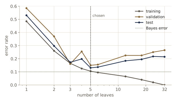
\[g(t) = \frac{R(t) - R(T_t)}{\lvert T_t \rvert - 1},\]the increase in training error per leaf removed. Weakest-link pruning computes \(g(t)\) for every internal node, collapses the node (or nodes) with the smallest value, and repeats on the smaller tree until only the root remains. As \(\alpha\) grows from zero this gives a nested sequence of trees, and one can show that each tree in the sequence minimizes \(R_\alpha\) over all subtrees for a whole interval of \(\alpha\) values. We then choose one tree from the short sequence by its validation error.
def resub_errors(t):
    """(misclassified training samples at the leaves of t, number of leaves)."""
    if is_leaf(t):
        return t["counts"].sum() - t["counts"].max(), 1
    eL, lL = resub_errors(t["left"])
    eR, lR = resub_errors(t["right"])
    return eL + eR, lL + lR

def g_value(t, n):
    R_t = (t["counts"].sum() - t["counts"].max()) / n
    R_sub, leaves = resub_errors(t)
    return (R_t - R_sub / n) / (leaves - 1)

def weakest_link(t, n):
    if is_leaf(t):
        return np.inf
    return min(g_value(t, n), weakest_link(t["left"], n), weakest_link(t["right"], n))

def as_leaf(t):
    return {"counts": t["counts"], "label": t["label"], "depth": t["depth"]}

def collapse(t, n, g_min):
    """Copy of t with every node whose g equals the minimum turned into a leaf."""
    if is_leaf(t):
        return t
    if g_value(t, n) <= g_min + 1e-12:
        return as_leaf(t)
    return {**t, "left": collapse(t["left"], n, g_min),
            "right": collapse(t["right"], n, g_min)}

def prune_sequence(tree):
    """[(alpha, tree), ...] from the full tree down to the root alone."""
    n = tree["counts"].sum()
    seq = [(0.0, tree)]
    while not is_leaf(seq[-1][1]):
        g_min = weakest_link(seq[-1][1], n)
        seq.append((g_min, collapse(seq[-1][1], n, g_min)))
    return seq

seq = prune_sequence(full_tree)
print("  alpha   leaves   train    val    test")
for alpha, t in seq:
    print(f"{alpha:7.4f}   {n_leaves(t):4d}   {error_rate(t, X_tr, y_tr):.3f}  "
          f"{error_rate(t, X_va, y_va):.3f}  {error_rate(t, X_te, y_te):.3f}")
val_key = lambda at: (error_rate(at[1], X_va, y_va), n_leaves(at[1]))  # ties: fewer leaves
alpha_best, pruned_tree = min(seq, key=val_key)
print(f"chosen by validation: alpha {alpha_best:.4f}, {n_leaves(pruned_tree)} leaves")
print(show_tree(pruned_tree))
  alpha   leaves   train    val    test
 0.0000     32   0.000  0.265  0.215
 0.0025     24   0.020  0.250  0.217
 0.0033     18   0.040  0.225  0.195
 0.0042     12   0.065  0.225  0.184
 0.0050      6   0.095  0.155  0.136
 0.0100      5   0.105  0.150  0.130
 0.0200      4   0.125  0.255  0.198
 0.0400      3   0.165  0.160  0.173
 0.0950      2   0.260  0.370  0.298
 0.2250      1   0.485  0.585  0.531
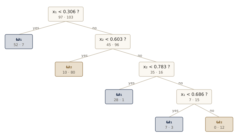
chosen by validation: alpha 0.0100, 5 leaves
x1 < 0.306 ?   counts [ 97 103]
    -> w1  counts [52  7]
    x2 < 0.603 ?   counts [45 96]
        -> w2  counts [10 80]
        x2 < 0.783 ?   counts [35 16]
            -> w1  counts [28  1]
            x1 < 0.686 ?   counts [ 7 15]
                -> w1  counts [7 3]
                -> w2  counts [ 0 12]
The sequence has only ten trees, so choosing among them is cheap. Validation picks the five-leaf tree, whose test error of 13% is close to the 10% Bayes error and far below the full tree’s. Its questions recover the true structure: the left strip \(x_1 < 0.31\) is \(\omega_1\), the lower box \(x_2 < 0.60\) is \(\omega_2\), and the upper-right corner is found by \(x_2 \ge 0.78\) and \(x_1 \ge 0.69\), all close to the true thresholds 0.35, 0.6, 0.8, and 0.7.
Pruning also rescues the exclusive-or problem, where stopping failed:
seq_x = prune_sequence(grow(X_xtr, y_xtr, 2, gini_imp))
xor_key = lambda at: (error_rate(at[1], X_xva, y_xva), n_leaves(at[1]))
_, xor_pruned = min(seq_x, key=xor_key)
for name, t in [("full tree", seq_x[0][1]), ("pruned", xor_pruned)]:
    print(f"{name:9s} {n_leaves(t):2d} leaves, "
          f"test error {error_rate(t, X_xte, y_xte):.3f}")
full tree 18 leaves, test error 0.138
pruned     8 leaves, test error 0.103
The pruned tree’s test error of about 10% compares with 50% for the stopped tree and 14% for the full one (the 5% label noise alone puts a floor at 5%). Its root question is still the odd edge split, which pruning cannot undo, but the splits below it find the quadrants.
In practice. Pruning costs more computation than stopping, since we grow the whole tree first, but for small and medium problems the cost is negligible and pruning is usually the better choice. It uses all the training data to grow the tree and avoids the horizon effect. A validation set (or cross-validation) is still needed to choose \(\alpha\); the sequence of candidate trees is short, so the choice is cheap.
A related method, reduced-error pruning, skips the \(\alpha\) sequence: working bottom-up, it collapses any internal node whose collapse does not increase the error on the validation set. It is simpler, but it uses the validation set both to shape the tree and to judge it. A third family prunes the rules read off a tree rather than its nodes; we meet it with C4.5 below.
Assigning leaf labels
When leaves are pure, each takes its category. After stopping or pruning, leaves are usually impure, and a leaf should take the category with the most training samples at that leaf, which minimizes the training error there. (With priors that differ between training and use, or with unequal costs, we will replace “most samples” by “smallest risk”.) A very small leaf impurity is not a virtue in itself; on noisy data it usually means the tree has memorized the noise.
Instability
Trees have a less pleasant property: they can change drastically when the training data change a little. Each split is a discrete, greedy choice, and every later choice depends on it, so a tiny change that flips which question wins at the root changes everything below. The cell builds a small 16-point set, moves one point by 0.05 in \(x_1\), and compares the two fully grown trees.
def tree_depths(t):
    return [t["depth"]] if is_leaf(t) else tree_depths(t["left"]) + tree_depths(t["right"])

gen_s = np.random.default_rng(21)
X_s = gen_s.random((16, 2))
X_s[8:] += 0.25                                   # second category shifted up and right
X_s = np.round(X_s, 2)
y_s = np.repeat([0, 1], 8)
X_s2 = X_s.copy()
X_s2[4, 0] += 0.05                                # move one point slightly

t_a, t_b = grow(X_s, y_s, 2, entropy_imp), grow(X_s2, y_s, 2, entropy_imp)
print(f"moved point {X_s[4]} -> {X_s2[4]}")
for name, t in [("original", t_a), ("moved", t_b)]:
    print(f"{name:8s} root question x{t['feat'] + 1} < {t['thr']:.3f}, "
          f"{n_leaves(t)} leaves, depth {max(tree_depths(t))}")
gg = np.linspace(0, 1.25, 126)
G = np.array([(a, b) for a in gg for b in gg])
print(f"fraction of the square [0, 1.25]^2 where the two trees disagree: "
      f"{np.mean(predict(t_a, G) != predict(t_b, G)):.3f}")
moved point [0.96 0.68] -> [1.01 0.68]
original root question x1 < 1.000, 5 leaves, depth 4
moved    root question x2 < 0.230, 5 leaves, depth 4
fraction of the square [0, 1.25]^2 where the two trees disagree: 0.448
Moving one point by 0.05 changed the root question from one feature to the other and relabeled 45% of the square. A nearest-neighbor rule trained on the same two sets would change only near the moved point. This instability is the price of greedy, discrete decisions. It is also the reason that averaging many trees grown on resampled data (bagging and its relatives, module 09 and Intro to ML, module 14) helps trees so much: the average of many unstable classifiers is much more stable than any one of them.
Computational complexity
Consider \(n\) training samples in \(d\) dimensions, two categories, axis-parallel splits, and entropy impurity. At the root we sort the samples on each feature, \(O(n \log n)\) per feature, and evaluate \(n - 1\) candidate thresholds per feature; with cumulative counts each evaluation costs \(O(1)\) for a fixed number of categories, so the root costs \(O(dn\log n)\). In the average case each split divides the samples roughly in half. Level 1 then has two nodes of \(n/2\) samples, costing \(O(dn\log(n/2))\) in total; level 2 costs \(O(dn\log(n/4))\); and there are \(O(\log n)\) levels, so growing the whole tree costs
\[\sum_{k=0}^{\log_2 n} O\left(dn\log\frac{n}{2^k}\right) = O\left(dn(\log n)^2\right)\]on average. Classifying a pattern costs one comparison per level, \(O(\log n)\), and a tree with one training sample per leaf has about \(1 + 2 + 4 + \dots + n/2 \approx n\) internal nodes, so storage is \(O(n)\). In the worst case, when each split peels off a single sample, depth becomes \(O(n)\) and growth becomes \(O(dn^2\log n)\), which is the safer rule of thumb; either way, training is far more expensive than classification. Two cheap speedups are common: only thresholds between neighboring samples of different categories can be optimal, so the others need not be evaluated, and sorting once at the root and passing sorted index lists down the tree removes the repeated sorts. With nominal attributes the search is over subsets of values instead, and the number of subsets grows exponentially with the number of values, so insight into the attributes matters more than clever code.
Feature choice
Like every classifier, a tree works best with the right features, and a monothetic tree is especially sensitive to the choice because it can only cut parallel to the axes. The usual preprocessing of numeric data applies. Principal components, for example, rotate the data onto its directions of largest variance, which often lines those axes up with the structure that matters. If the good directions differ from one part of feature space to another, no single rotation will do, and we need questions that can take any direction.
Multivariate decision trees
A multivariate (or oblique) tree asks linear questions, “is \(\mathbf{w}^{t}\mathbf{x} < w_0\)?”, at its nodes. Any method for training a linear discriminant from module 05 can supply \(\mathbf{w}\). The node data are almost never linearly separable, so a least-squares (LMS) fit is more robust here than the perceptron family, even though it does not minimize the error rate. We use the minimum-squared-error solution: augment each sample to \(\mathbf{y} = (1, \mathbf{x})\), set a target of \(+1\) for one category and \(-1\) for the other, solve \(\mathbf{Y}\mathbf{a} \approx \mathbf{b}\) by least squares, and keep the weight part of \(\mathbf{a}\) as the direction. The threshold along that direction is then chosen by impurity, reusing best_split on the one-dimensional projections \(z = \mathbf{w}^{t}\mathbf{x}\). Training such a node is slower than an axis-parallel search near the root, where there are many samples, but classification stays fast: one inner product per level.
Note. DHS write the transpose with a superscript \(t\), as in \(\mathbf{w}^{t}\mathbf{x}\), and name categories \(\omega_1, \dots, \omega_c\). The ML notes follow Bishop and write \(\mathbf{w}^{\mathrm{T}}\mathbf{x}\) and \(\mathcal{C}_1, \dots, \mathcal{C}_K\) for the same things.
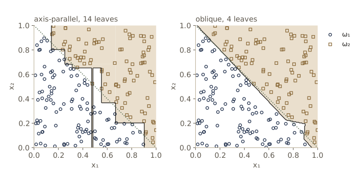
Our test is the simplest case where axis-parallel splits struggle: two categories separated by the diagonal \(x_1 + x_2 = 1\), with no label noise.
def make_diag(n, gen):
    X = gen.random((n, 2))
    return X, (X[:, 0] + X[:, 1] > 1).astype(int)

gen_d = np.random.default_rng(11)
X_dtr, y_dtr = make_diag(200, gen_d)
X_dte, y_dte = make_diag(5000, gen_d)

def lms_direction(X, y):
    """Weight part of the least-squares solution of Y a = b, b = +1 / -1 (module 05)."""
    Y = np.column_stack([np.ones(len(X)), X])
    b = np.where(y == 1, 1.0, -1.0)
    a, *_ = np.linalg.lstsq(Y, b, rcond=None)
    return a[1:]

def grow_oblique(X, y, c, impurity=gini_imp, depth=0, max_depth=20):
    """Two-category oblique tree: LMS direction at each node, threshold by impurity."""
    counts = np.bincount(y, minlength=c)
    node = {"counts": counts, "label": int(np.argmax(counts)), "depth": depth}
    if np.count_nonzero(counts) <= 1 or depth >= max_depth:
        return node
    w = lms_direction(X, y)
    z = (X @ w)[:, None]                      # project onto w, then a 1-D search
    gain, _, thr = best_split(z, y, c, impurity)
    if thr is None:
        return node
    go = z[:, 0] < thr
    node.update(w=w, thr=thr,
                left=grow_oblique(X[go], y[go], c, impurity, depth + 1, max_depth),
                right=grow_oblique(X[~go], y[~go], c, impurity, depth + 1, max_depth))
    return node

def predict_oblique(t, X):
    out = np.empty(len(X), dtype=int)
    def route(t, idx):
        if "w" not in t:
            out[idx] = t["label"]
            return
        m = X[idx] @ t["w"] < t["thr"]
        route(t["left"], idx[m])
        route(t["right"], idx[~m])
    route(t, np.arange(len(X)))
    return out

def n_leaves_oblique(t):
    if "w" not in t:
        return 1
    return n_leaves_oblique(t["left"]) + n_leaves_oblique(t["right"])

t_axis = grow(X_dtr, y_dtr, 2, gini_imp)
t_obl = grow_oblique(X_dtr, y_dtr, 2)
print(f"axis-parallel: {n_leaves(t_axis):2d} leaves, test error "
      f"{error_rate(t_axis, X_dte, y_dte):.4f}")
print(f"oblique:       {n_leaves_oblique(t_obl):2d} leaves, test error "
      f"{np.mean(predict_oblique(t_obl, X_dte) != y_dte):.4f}")
w, thr = t_obl["w"], t_obl["thr"]
print(f"root question: {w[0]:.3f} x1 + {w[1]:.3f} x2 < {thr:.3f}"
      f"   (i.e. x1 + {w[1] / w[0]:.3f} x2 < {thr / w[0]:.3f})")

R45 = np.array([[1.0, 1.0], [-1.0, 1.0]]) / np.sqrt(2)     # rotate the axes by 45 degrees
t_rot = grow(X_dtr @ R45.T, y_dtr, 2, gini_imp)
print(f"axis-parallel after rotating the features: {n_leaves(t_rot)} leaves")
axis-parallel: 14 leaves, test error 0.0666
oblique:        4 leaves, test error 0.0224
root question: 2.047 x1 + 1.927 x2 < 1.952   (i.e. x1 + 0.941 x2 < 0.953)
axis-parallel after rotating the features: 2 leaves
The axis-parallel tree approximates the diagonal with a staircase of fourteen leaves and still makes about three times as many test errors as the oblique tree. The oblique root question is almost exactly the true boundary; the few extra leaves below it only clean up the small misfit of the least-squares direction. Rotating the features by 45 degrees, the “proper feature” fix, reduces the axis-parallel tree to a single question.
Priors and costs
So far each training sample has counted once, which quietly assumes that the category frequencies in the training set are the ones the classifier will meet in use, and that all errors cost the same. Neither need be true. Following the decision theory of module 02, let \(P'(\omega_j)\) be the priors in use and \(\lambda_{ij} = \lambda(\alpha_i \mid \omega_j)\) the cost of deciding \(\omega_i\) when the truth is \(\omega_j\).
Priors. If the training set has category frequencies \(\hat{P}(\omega_j)\), giving each sample of \(\omega_j\) the weight \(P'(\omega_j)/\hat{P}(\omega_j)\) makes every weighted class count, and hence every impurity and every leaf’s class frequencies, what they would have been under the priors in use. This is why best_split and grow accept sample weights.
Costs at the leaves. With class frequencies \(P(\omega_j \mid N)\) at a leaf, the label should minimize the conditional risk rather than the error,
\[\text{label}(N) = \arg\min_i \sum_{j=1}^{c} \lambda_{ij}\, P(\omega_j \mid N).\]Costs in the impurity. DHS suggest the weighted Gini impurity \(i(N) = \sum_{i,j} \lambda_{ij} P(\omega_i)P(\omega_j)\) for growing the tree. Be aware of what it does with two categories: the sum is \((\lambda_{12} + \lambda_{21})P(\omega_1)P(\omega_2)\), a constant multiple of the ordinary Gini impurity, so it selects exactly the same splits. For two categories a more effective way to bring the costs into the growth is to fold them into the sample weights as well, weighting each sample of \(\omega_j\) by \(\lambda_{ij}\), \(i \neq j\), the cost of misclassifying it. The weighted majority at a leaf is then exactly the minimum-risk label. This device is often called altered priors.
The cell tests these ideas on two overlapping Gaussian categories. The training set is balanced, but in use \(P'(\omega_1) = 0.8\) and \(P'(\omega_2) = 0.2\), and missing an \(\omega_2\) pattern costs six times as much as a false alarm. All trees stop at 10 samples per leaf.
def make_gauss(n1, n2, gen):
    X = np.vstack([gen.normal(0.0, 1.0, (n1, 2)), gen.normal(1.5, 1.0, (n2, 2))])
    return X, np.repeat([0, 1], [n1, n2])

gen_p = np.random.default_rng(5)
X_btr, y_btr = make_gauss(300, 300, gen_p)         # balanced training set
X_bte, y_bte = make_gauss(8000, 2000, gen_p)       # data in use: P'(w1) = 0.8
P_use = np.array([0.8, 0.2])
P_hat = np.bincount(y_btr) / len(y_btr)
Lam = np.array([[0.0, 6.0],                        # lambda_ij: decide w_i, truth w_j
                [1.0, 0.0]])

def weighted_gini(Lam):
    return lambda P: np.einsum("...i,ij,...j->...", P, Lam, P)

P = np.array([0.3, 0.7])
print(f"weighted Gini / Gini = {weighted_gini(Lam)(P) / gini_imp(P):.2f} "
      f"(= (lambda12 + lambda21) / 2)")

def min_risk_labels(t, Lam):
    lab = int(np.argmin(Lam @ (t["counts"] / t["counts"].sum())))
    if is_leaf(t):
        return {**t, "label": lab}
    return {**t, "label": lab, "left": min_risk_labels(t["left"], Lam),
            "right": min_risk_labels(t["right"], Lam)}

def avg_cost(pred, y):
    return float(Lam[pred, y].mean())

w_prior = (P_use / P_hat)[y_btr]
w_altered = w_prior * Lam.sum(axis=0)[y_btr]    # column sum = cost of misclassifying w_j
trees = {"plain": grow(X_btr, y_btr, 2, gini_imp, min_leaf=10),
         "prior weights": grow(X_btr, y_btr, 2, gini_imp, min_leaf=10, w=w_prior)}
trees["prior weights + min-risk labels"] = min_risk_labels(trees["prior weights"], Lam)
trees["altered priors"] = grow(X_btr, y_btr, 2, gini_imp, min_leaf=10, w=w_altered)
for name, t in trees.items():
    pred = predict(t, X_bte)
    print(f"{name:32s} error {np.mean(pred != y_bte):.3f}   "
          f"average cost {avg_cost(pred, y_bte):.3f}")

def gauss_logpdf(X, mu):                 # unit-covariance Gaussian, for the Bayes rule
    return -0.5 * ((X - mu) ** 2).sum(axis=1) - np.log(2 * np.pi)
r1 = np.log(0.8) + gauss_logpdf(X_bte, 0.0)
r2 = np.log(0.2) + gauss_logpdf(X_bte, 1.5)
risk_rule = (np.log(6) + r2 > r1).astype(int)     # decide w2 if 6 P(w2|x) > P(w1|x)
print(f"Bayes rule: error {np.mean((r2 > r1) != y_bte):.3f}   "
      f"minimum-risk rule: average cost {avg_cost(risk_rule, y_bte):.3f}")
weighted Gini / Gini = 3.50 (= (lambda12 + lambda21) / 2)
plain                            error 0.151   average cost 0.353
prior weights                    error 0.115   average cost 0.529
prior weights + min-risk labels  error 0.171   average cost 0.331
altered priors                   error 0.210   average cost 0.323
Bayes rule: error 0.107   minimum-risk rule: average cost 0.285
Weighting by the priors in use cuts the error from 15% to 11.5%, close to the Bayes error of 10.7%. But it raises the average cost, because the rarer \(\omega_2\) is now predicted less often and each miss costs 6. Labeling the leaves by minimum risk reverses this: the error goes up (borderline leaves are called \(\omega_2\) on purpose) and the average cost goes down. Folding the costs into the weights, so that the splits themselves are chosen with the costs in mind, gives the lowest cost of the tree variants, though still above the minimum-risk rule computed from the true densities.
Missing attributes
Real data often have gaps. During training, the simplest remedy, discarding every deficient pattern (one with a missing value), wastes data. A better one keeps the tree-growing procedure unchanged but computes each candidate’s impurity drop using only the samples for which that attribute is present, so that different features are judged on slightly different sample sets; the best drop still wins.
Classification with a missing value is harder: if a test pattern lacks \(x_i\), the question “is \(x_i < x_{is}\)?” cannot be answered. CART’s answer is to store, at each internal node, an ordered list of surrogate splits. A surrogate is a question on a different attribute chosen to imitate the primary split as closely as possible. Its quality is its predictive association with the primary split: the number of training samples at the node that both splits send left, plus the number that both send right. The first surrogate is the question with the highest association, the second the best one on yet another attribute, and so on. At classification time a pattern that lacks the primary attribute uses the first surrogate whose attribute it has. In effect this imputes the missing value from the attribute most strongly associated with it, locally at each node.
Finding the best surrogate on attribute \(x_k\) is a one-dimensional search like best_split: sort the node’s samples on \(x_k\), and for every cut position count how many of the primary split’s left-goers fall below the cut and how many right-goers fall above it.
def surrogate_splits(X, go_left, j_primary):
    """[(agreement, k, thr), ...] best 'x_k < thr' for each other attribute, best first."""
    out = []
    for k in range(X.shape[1]):
        if k == j_primary:
            continue
        order = np.argsort(X[:, k], kind="stable")
        xs, gl = X[order, k], go_left[order]
        # cut after the first m samples (m = 0..n): agreements on the left and on the right
        left_hits = np.concatenate([[0], np.cumsum(gl)])
        right_hits = (~gl).sum() - np.concatenate([[0], np.cumsum(~gl)])
        agree = left_hits + right_hits
        valid = np.concatenate([[True], xs[1:] > xs[:-1], [True]])
        m = int(np.argmax(np.where(valid, agree, -1)))
        thr = -np.inf if m == 0 else np.inf if m == len(xs) else 0.5 * (xs[m - 1] + xs[m])
        out.append((int(agree[m]), k, float(thr)))
    return sorted(out, reverse=True)

def add_surrogates(t, X):
    """Store surrogates and branch sizes at every internal node (X: the node's samples)."""
    if is_leaf(t):
        return
    go = X[:, t["feat"]] < t["thr"]
    t["surrogates"] = surrogate_splits(X, go, t["feat"])
    t["n_left"], t["n_right"] = int(go.sum()), int((~go).sum())
    add_surrogates(t["left"], X[go])
    add_surrogates(t["right"], X[~go])

def predict_missing(t, X, use_surrogates=True):
    """NaN marks a missing value. Without surrogates, go to the larger branch."""
    out = np.empty(len(X), dtype=int)
    for r, x in enumerate(X):
        node = t
        while not is_leaf(node):
            if not np.isnan(x[node["feat"]]):
                left = x[node["feat"]] < node["thr"]
            else:
                usable = [(k, s) for _, k, s in node["surrogates"]
                          if use_surrogates and not np.isnan(x[k])]
                if usable:
                    left = x[usable[0][0]] < usable[0][1]         # first usable surrogate
                else:
                    left = node["n_left"] >= node["n_right"]     # larger branch
            node = node["left"] if left else node["right"]
        out[r] = node["label"]
    return out
The test data have three features: the category depends on \(x_1\) alone (with 5% label noise), \(x_2\) is \(x_1\) plus a little noise, and \(x_3\) is only half \(x_1\). We grow a tree on complete training data, compute surrogates, and then delete \(x_1\) from every test pattern.
def make_corr(n, gen, flip=0.05):
    x1 = gen.random(n)
    x2 = x1 + gen.normal(0.0, 0.1, n)
    x3 = 0.5 * x1 + 0.5 * gen.random(n)
    y = (x1 > 0.5).astype(int)
    noisy = gen.random(n) < flip
    return np.column_stack([x1, x2, x3]), np.where(noisy, 1 - y, y)

gen_m = np.random.default_rng(14)
X_mtr, y_mtr = make_corr(300, gen_m)
X_mte, y_mte = make_corr(3000, gen_m)
t_m = grow(X_mtr, y_mtr, 2, entropy_imp, split_ok=mdl_ok(3))       # MDL stopping rule
add_surrogates(t_m, X_mtr)
print(show_tree(t_m, names=("x1", "x2", "x3")), end="")
print("root surrogates (agreement out of 300, feature, threshold):")
for a, k, s in t_m["surrogates"]:
    print(f"   {a:3d}   x{k + 1} < {s:.3f}")

X_no1 = X_mte.copy(); X_no1[:, 0] = np.nan
X_no12 = X_no1.copy(); X_no12[:, 1] = np.nan
err = lambda pred: np.mean(pred != y_mte)
print(f"test error, complete patterns:   {error_rate(t_m, X_mte, y_mte):.3f}")
print(f"x1 missing, surrogates:          {err(predict_missing(t_m, X_no1)):.3f}")
print(f"x1 and x2 missing, surrogates:   {err(predict_missing(t_m, X_no12)):.3f}")
print(f"x1 missing, larger branch:       {err(predict_missing(t_m, X_no1, False)):.3f}")
x1 < 0.496 ?   counts [139 161]
    -> w1  counts [134   8]
    -> w2  counts [  5 153]
root surrogates (agreement out of 300, feature, threshold):
   273   x2 < 0.462
   218   x3 < 0.634
test error, complete patterns:   0.060
x1 missing, surrogates:          0.128
x1 and x2 missing, surrogates:   0.322
x1 missing, larger branch:       0.490
The description-length rule stops after one question, the primary split on \(x_1\) near 0.5, which is the true boundary. Its first surrogate, on the close copy \(x_2\), sends 273 of the 300 training samples the same way as the primary split; the second, on \(x_3\), agrees on 218. With \(x_1\) gone, the surrogates keep the error far below the roughly 50% we get by sending every pattern down the larger branch, and even with two of the three features gone the weakly associated \(x_3\) still helps. Note that the surrogate thresholds are chosen to imitate the primary split, not to reduce impurity: the best \(x_3\) question for mimicking the primary split need not be the best \(x_3\) question for separating the categories.
Two related ideas deserve a mention. Virtual values replace a missing attribute by its most likely value (for example, the most common value among training samples at the node). And sometimes the absence itself is informative: a lab test that was never ordered may say something about what the physician suspected. Then “missing” can be treated as one more attribute value, or an indicator of missingness can be added as a feature.
Other tree methods
The components above — impurity, stopping, pruning, leaf labels, missing values — can be combined freely, and most tree algorithms are particular combinations. Two classic ones come from Quinlan’s work.
ID3
ID3 is designed for nominal attributes. Real-valued attributes must first be binned into intervals, each treated as an unordered value. A node that splits on attribute \(j\) gets one branch per value, a branching factor \(B_j\) equal to the number of values, and an attribute once used is not used again below that node, so the depth is at most the number of attributes. Growth continues until the nodes are pure or no attributes remain; the original algorithm does not prune, though any of the pruning methods above can be added.
For a \(B\)-way split that sends fractions \(P_1, \dots, P_B\) of the samples to children \(N_1, \dots, N_B\), the natural generalization of the impurity drop is the information gain
\[\Delta i(s) = i(N) - \sum_{k=1}^{B} P_k\, i(N_k).\]It has a bias: splits with more branches reduce impurity more, even on random data, because small children are purer by chance. The extreme case is an attribute that is different for every sample, such as a serial number; splitting on it makes every child pure and achieves the largest possible gain, and it is useless for new patterns. The gain ratio corrects for this by dividing by the entropy of the split proportions themselves, the information in the split regardless of the classes:
\[\Delta i_B(s) = \frac{\Delta i(s)}{-\sum_{k=1}^{B} P_k \log_2 P_k}.\]We apply both criteria to 24 of the 36 possible houseplants, labeled by the rule tree from the start of the module. To show the bias we also give every plant a unique tag.
gen_n = np.random.default_rng(36)
train_idx = gen_n.choice(len(all_plants), 24, replace=False)
plants = [dict(all_plants[i], tag=f"p{r:02d}") for r, i in enumerate(train_idx)]
plant_labels = [classify_nominal(plant_tree, p) for p in plants]

def label_entropy(labels):
    cnt = np.array(list(Counter(labels).values()), float)
    return float(entropy_imp(cnt / cnt.sum()))

def gain_and_split_info(samples, labels, a):
    groups = {}
    for s, lab in zip(samples, labels):
        groups.setdefault(s[a], []).append(lab)
    Pk = np.array([len(g) for g in groups.values()], float) / len(labels)
    children = sum(p * label_entropy(g) for p, g in zip(Pk, groups.values()))
    gain = label_entropy(labels) - children
    return gain, float(entropy_imp(Pk))

print(Counter(plant_labels), f"  root entropy {label_entropy(plant_labels):.4f} bits")
print("attribute   B   gain    split info   gain ratio")
for a in ["light", "water", "pot", "humidity", "tag"]:
    g, si = gain_and_split_info(plants, plant_labels, a)
    B = len(set(p[a] for p in plants))
    print(f"{a:9s} {B:3d}   {g:.4f}   {si:.4f}       {g / si:.4f}")
Counter({'struggles': 17, 'thrives': 7})   root entropy 0.8709 bits
attribute   B   gain    split info   gain ratio
light       3   0.2391   1.5774       0.1516
water       3   0.4374   1.5343       0.2851
pot         2   0.0061   1.0000       0.0061
humidity    2   0.0290   0.9799       0.0296
tag        24   0.8709   4.5850       0.1899
Information gain prefers the tag, which reaches the maximum possible value, the full root entropy. The gain ratio divides it by the large entropy of a 24-way split and correctly prefers water. The ID3 recursion itself is short:
def id3(samples, labels, attrs, criterion="ratio"):
    majority = Counter(labels).most_common(1)[0][0]
    if len(set(labels)) == 1 or not attrs:
        return majority
    def score(a):
        g, si = gain_and_split_info(samples, labels, a)
        return g / si if (criterion == "ratio" and si > 0) else g
    best = max(attrs, key=score)
    node = {"attr": best, "branches": {}, "majority": majority}
    for v in sorted(set(s[best] for s in samples)):
        keep = [r for r, s in enumerate(samples) if s[best] == v]
        node["branches"][v] = id3([samples[r] for r in keep], [labels[r] for r in keep],
                                  [b for b in attrs if b != best], criterion)
    return node

def classify_id3(tree, x):
    while isinstance(tree, dict):
        if x[tree["attr"]] not in tree["branches"]:      # value never seen at this node
            return tree["majority"]
        tree = tree["branches"][x[tree["attr"]]]
    return tree

for crit in ["gain", "ratio"]:
    t = id3(plants, plant_labels, ["light", "water", "pot", "humidity", "tag"], crit)
    print(f"root attribute by {crit}: {t['attr']}")
t_id3 = id3(plants, plant_labels, ["light", "water", "pot", "humidity"], "ratio")
for conds, lab in tree_rules(t_id3):
    print(f"   {lab:9s} IF", " AND ".join(a + "=" + v for a, v in conds))
unseen = [p for r, p in enumerate(all_plants) if r not in set(train_idx)]
acc = np.mean([classify_id3(t_id3, p) == classify_nominal(plant_tree, p) for p in unseen])
print(f"agreement with the true rule on the {len(unseen)} unseen plants: {acc:.3f}")
root attribute by gain: tag
root attribute by ratio: water
   struggles IF water=daily
   struggles IF water=sparse
   thrives   IF water=weekly AND light=bright
   struggles IF water=weekly AND light=low
   thrives   IF water=weekly AND light=medium
agreement with the true rule on the 12 unseen plants: 0.833
With the gain ratio, ID3 finds the water node and, under weekly watering, the light node of the true rule, and it ignores the irrelevant pot. It misses the rare third path (daily watering, humid air, bright light) because no such plant is in the 24 training samples, so it gets two of the twelve unseen plants wrong. tree_rules from the start of the module reads the ID3 tree as well, since both use the same nested-dictionary format.
C4.5
C4.5, ID3’s successor, is probably the most widely used of Quinlan’s tree algorithms. It handles real-valued attributes with binary threshold questions, as CART does, keeps multiway splits with the gain ratio for nominal attributes, and prunes with heuristics based on the statistical significance of splits. Two further features distinguish it.
Missing values by weighted descent. C4.5 stores no surrogates. When a test pattern reaches a node whose attribute it lacks, it follows all the branches, weighting each by the fraction of training samples at the node that went that way, and combines the class distributions of all the leaves reached with those weights. This is cheaper in storage than surrogates, but it ignores the correlations between attributes that surrogates exploit. On the missing-\(x_1\) problem above it cannot recover:
def predict_fractional(t, x):
    """Class distribution for one pattern; a missing value sends it down both branches."""
    if is_leaf(t):
        return t["counts"] / t["counts"].sum()
    if np.isnan(x[t["feat"]]):
        pL = t["n_left"] / (t["n_left"] + t["n_right"])
        return (pL * predict_fractional(t["left"], x)
                + (1 - pL) * predict_fractional(t["right"], x))
    return predict_fractional(t["left"] if x[t["feat"]] < t["thr"] else t["right"], x)

pred_frac = np.array([np.argmax(predict_fractional(t_m, x)) for x in X_no1])
print(f"x1 missing, weighted descent: test error {np.mean(pred_frac != y_mte):.3f}")
x1 missing, weighted descent: test error 0.490
With the root attribute missing, the weighted descent can do no better than the training class proportions, which is a coin flip here. It shines instead when the missing attribute is one of many weak ones deep in the tree.
Rule post-pruning. C4.5 can convert a tree into rules, one per leaf, each the conjunction of the tests on the path to that leaf, and prune the rules instead of the tree. Some antecedents are logically redundant (a path that asks \(x_2 \ge 0.60\) and later \(x_2 \ge 0.78\) needs only the second), and removing them changes nothing. Others are statistically unnecessary, and dropping them may even improve accuracy. Because each rule is pruned on its own, a test near the root can be dropped from one rule while it stays in another, which node pruning cannot do: a node is either kept for all the patterns that pass through it or removed for all of them.
The next cell implements a simple version. It tightens each rule logically, then repeatedly drops the antecedent whose removal most improves the rule’s estimated accuracy on the validation set (a Laplace-corrected fraction of covered validation samples with the rule’s label), stopping when every removal would lower it. The rules are then applied in order of estimated accuracy, and a pattern no rule covers gets the training majority. We start from the twelve-leaf tree of the pruning sequence, which still has some overfitting to remove.
def rules_from_tree(t, conds=()):
    if is_leaf(t):
        return [(list(conds), t["label"])]
    j, thr = t["feat"], t["thr"]
    return (rules_from_tree(t["left"], conds + ((j, "<", thr),)) +
            rules_from_tree(t["right"], conds + ((j, ">=", thr),)))

def tighten(conds):
    """Keep the tightest bound per feature and direction: logically equivalent."""
    best = {}
    for j, op, thr in conds:
        old = best.get((j, op))
        if old is None or (thr < old if op == "<" else thr > old):
            best[(j, op)] = thr
    return [(j, op, thr) for (j, op), thr in sorted(best.items())]

def covers(conds, X):
    m = np.ones(len(X), dtype=bool)
    for j, op, thr in conds:
        m &= (X[:, j] < thr) if op == "<" else (X[:, j] >= thr)
    return m

def rule_accuracy(conds, label, X, y):
    m = covers(conds, X)
    return (np.sum(y[m] == label) + 1) / (m.sum() + 2)      # Laplace correction

def prune_rule(conds, label, X, y):
    conds = list(conds)
    while conds:
        acc, k = max((rule_accuracy(conds[:k] + conds[k + 1:], label, X, y), k)
                     for k in range(len(conds)))
        if acc < rule_accuracy(conds, label, X, y):
            break
        conds.pop(k)
    return conds

def classify_rules(rules, X, default, Xv, yv):
    ordered = sorted(rules, key=lambda r: -rule_accuracy(r[0], r[1], Xv, yv))
    out, done = np.full(len(X), default), np.zeros(len(X), dtype=bool)
    for conds, lab in ordered:
        m = covers(conds, X) & ~done
        out[m], done = lab, done | m
    return out

def fmt(conds):
    return " AND ".join(f"x{j + 1} {op} {thr:.3f}" for j, op, thr in conds) or "(always)"

tree12 = seq[3][1]
rules = rules_from_tree(tree12)
pruned_rules = [(prune_rule(tighten(c), lab, X_va, y_va), lab) for c, lab in rules]
n_ante = lambda rs: sum(len(c) for c, _ in rs)
print(f"{len(rules)} rules; antecedents: {n_ante(rules)} as read off the tree, "
      f"{n_ante([(tighten(c), lab) for c, lab in rules])} after tightening, "
      f"{n_ante(pruned_rules)} after pruning")
for r in (7, 8, 11):
    print(f"w{rules[r][1] + 1} IF {fmt(rules[r][0])}")
    print(f"     -> IF {fmt(pruned_rules[r][0])}")
default = int(np.argmax(np.bincount(y_tr)))
pred_rules = classify_rules(pruned_rules, X_te, default, X_va, y_va)
print(f"test error: 12-leaf tree {error_rate(tree12, X_te, y_te):.3f},  "
      f"its pruned rules {np.mean(pred_rules != y_te):.3f}")
12 rules; antecedents: 49 as read off the tree, 33 after tightening, 23 after pruning
w1 IF x1 >= 0.306 AND x2 >= 0.603 AND x2 < 0.783
     -> IF x2 < 0.783 AND x2 >= 0.603
w2 IF x1 >= 0.306 AND x2 >= 0.603 AND x2 >= 0.783 AND x1 < 0.686 AND x1 < 0.340
     -> IF x1 < 0.340 AND x1 >= 0.306 AND x2 >= 0.783
w2 IF x1 >= 0.306 AND x2 >= 0.603 AND x2 >= 0.783 AND x1 >= 0.686
     -> IF x1 >= 0.686
test error: 12-leaf tree 0.184,  its pruned rules 0.136
Tightening removes about a third of the antecedents without changing anything; pruning then removes more. The first rule shown loses the root test \(x_1 \ge 0.306\) altogether: the band \(0.603 \le x_2 < 0.783\) is \(\omega_1\) across the whole square, and the rule now says so. The rule set generalizes better than the tree it came from.
Which tree classifier is best?
Rather than ranking CART, ID3, and C4.5 as packages, it is more useful to compare their components, since any reasonable choice of impurity, stopping rule, pruning method, and missing-value strategy can be combined with any other. A few rules of thumb:
- Use what you know about the features. Binning real values, as early versions of ID3 did, discards their order and should be a last resort.
- Entropy impurity is a sensible default; Gini behaves almost the same. Misclassification impurity should not be used for growing.
- Pruning generally beats stopped splitting, because it uses all the training data and avoids the horizon effect, at a computational cost that matters only for large data sets.
- Rule pruning helps most when the data really were generated by crisp rules, and less on noisy, statistical problems.
- Some simple concepts are awkward for trees. “More than half of the \(d\) binary attributes are 1” needs a tree that enumerates combinations, while a single linear threshold unit represents it exactly.
No tree algorithm dominates the others on all problems, which is an instance of the no-free-lunch theorem of module 09. On many problems trees reach accuracy comparable to neural networks and nearest-neighbor rules, and they are the natural choice when the data are nominal or mixed, or when the classifier must be read and checked by people.
Recognition with strings
Many patterns are sequences: the letters of a word, the bases of a gene, the phoneme labels a speech front end assigns to successive 10-ms frames, or the stroke types an earlier classifier finds in handwriting. The elements are called characters (or letters, or symbols) and come from a finite alphabet \(\mathcal{A}\), such as \(\{\mathrm{A}, \mathrm{C}, \mathrm{G}, \mathrm{T}\}\) or the 26 English letters. A string (or word) is a finite sequence of characters, a particularly long string is called a text, and a contiguous piece of a string is a factor (substring): “ATT” is a factor of “GATTACA”. Strings are nominal twice over: their characters have no metric, and two strings need not have the same length, so they are not vectors at all. Four problems matter most in pattern recognition:
- String matching: is \(\mathbf{x}\) a factor of the text, and where?
- Edit distance: what is the smallest number of character insertions, deletions, and substitutions that turns \(\mathbf{x}\) into \(\mathbf{y}\)?
- String matching with errors: where in the text is there a factor closest to \(\mathbf{x}\) in edit distance?
- String matching with a don’t-care symbol: string matching where a special symbol matches any character.
Exact matching is template matching in its purest form: counting occurrences of keywords, for instance, is a crude but real way to sort documents by topic. Edit distance turns the nearest-neighbor rule of module 04 into a classifier for strings: store labeled prototype strings and give a new string the label of the nearest one. Matching with errors searches for misspelled or mutated versions of a target, and the don’t-care symbol expresses known gaps, such as an inert stretch between two important motifs of a DNA sequence. The ideas are simple; the work is in making them fast enough for texts of millions or billions of characters.
String matching
Let the text have \(n\) characters and the pattern \(\mathbf{x}\) have \(m \le n\). A shift \(s\) aligns the first character of \(\mathbf{x}\) with character \(s + 1\) of the text (with 0-based indexing in code, character \(s\)). A shift is valid if every character of \(\mathbf{x}\) equals the text character aligned with it, and in string matching we want every valid shift.
The naive algorithm tries every shift \(s = 0, 1, \dots, n - m\) and compares characters left to right until a mismatch. In the worst case (think of \(\mathbf{x}\) = “aaab” in a text of a’s) it makes \(m\) comparisons at each of \(n - m + 1\) shifts, \(O((n - m + 1)m)\) in all. On random text it is much better, since most shifts fail at the first or second character. Its real weakness is that it forgets everything it learned at one shift when it moves to the next.
The Boyer–Moore algorithm keeps that information. It compares characters of \(\mathbf{x}\) from right to left, and when a mismatch occurs it moves the shift forward by the larger of two safe amounts, each computed from tables built once from \(\mathbf{x}\):
- The bad-character heuristic looks at the text character that caused the mismatch, the bad character. If it does not occur in \(\mathbf{x}\) at all, no alignment that covers it can succeed, and the pattern can jump past it entirely. Otherwise the shift moves so that the rightmost occurrence of that character in \(\mathbf{x}\) lines up with it. The table is the last-occurrence function \(F(c)\), the position of the rightmost \(c\) in \(\mathbf{x}\) (0 if absent, in 1-based positions). A mismatch at pattern position \(j\) proposes a shift increment of \(j - F(c)\).
- The good-suffix heuristic looks at the characters that did match, the good suffix (a suffix of \(\mathbf{x}\) is a factor containing its last character, a prefix one containing its first). The shift moves so that the next occurrence of that suffix inside \(\mathbf{x}\) (or the longest prefix of \(\mathbf{x}\) that matches the end of it) lines up with the matched text. The table \(G(j)\) stores the resulting increment for a mismatch at each position \(j\), and \(G(0)\) gives the increment after a complete match.
Each proposal is safe on its own, since neither can skip a valid shift, so their maximum is too. The bad-character increment can be zero or negative (when the rightmost occurrence of the bad character lies to the right of the mismatch); the good-suffix increment is always at least 1, so the maximum always makes progress. We build \(G\) by brute force directly from its definition, which is fine for short patterns (efficient \(O(m)\) constructions exist but are harder to read). The version below uses the stronger form of the rule, which also requires the character before the re-aligned suffix to differ from the one that just mismatched.
def naive_match(x, text):
    shifts, comps = [], 0
    for s in range(len(text) - len(x) + 1):
        j = 0
        while j < len(x):
            comps += 1
            if x[j] != text[s + j]:
                break
            j += 1
        if j == len(x):
            shifts.append(s)
    return shifts, comps

def last_occurrence(x):
    """F(c) = rightmost 1-based position of c in x (characters not in x: 0)."""
    return {c: j + 1 for j, c in enumerate(x)}

def good_suffix(x):
    """G[j]: smallest safe increment after a mismatch at 1-based j (j = 0: full match)."""
    m = len(x)
    G = [0] * (m + 1)
    for j in range(m + 1):                       # x[j+1..m] (1-based) has matched
        for k in range(1, m + 1):
            suffix_ok = all(i - k < 1 or x[i - k - 1] == x[i - 1]
                            for i in range(j + 1, m + 1))
            differs = j == 0 or j - k < 1 or x[j - k - 1] != x[j - 1]
            if suffix_ok and differs:
                G[j] = k
                break
    return G

def boyer_moore(x, text, use_good_suffix=True):
    m, n = len(x), len(text)
    F, G = last_occurrence(x), good_suffix(x)
    shifts, comps, s = [], 0, 0
    while s <= n - m:
        j = m                                    # compare right to left, 1-based j
        while j > 0:
            comps += 1
            if x[j - 1] != text[s + j - 1]:
                break
            j -= 1
        if j == 0:
            shifts.append(s)
            s += G[0]
        else:
            bad_char = j - F.get(text[s + j - 1], 0)
            s += max(G[j] if use_good_suffix else 1, bad_char)
    return shifts, comps

print("F for 'tandem':", last_occurrence("tandem"))
print("G for 'abcab': ", good_suffix("abcab"))
F for 'tandem': {'t': 1, 'a': 2, 'n': 3, 'd': 4, 'e': 5, 'm': 6}
G for 'abcab':  [3, 3, 3, 3, 5, 1]
For “abcab”, a mismatch at the last position (\(j = 5\), nothing matched yet) allows an increment of 1, while after a full match (\(G(0)\)) the pattern can move by 3, because the suffix “ab” reappears as its prefix. We test the algorithm on two kinds of text: random DNA, and text made of words drawn from a small vocabulary full of near-misses for the pattern.
gen_t = np.random.default_rng(55)
dna = "".join(gen_t.choice(list("ACGT"), 20000))
vocab = ["class", "classes", "classify", "classifying", "classifier", "clause",
         "glass", "cross", "tree", "split", "node", "leaf", "impurity", "prune",
         "string", "grammar"]
words = "_".join(gen_t.choice(vocab, 3000))

cases = [("GATTACA", dna), ("ACGTACGTAC", dna), ("classifier", words), ("impurity", words)]
for x, text in cases:
    s_naive, c_naive = naive_match(x, text)
    s_bc, c_bc = boyer_moore(x, text, use_good_suffix=False)
    s_bm, c_bm = boyer_moore(x, text)
    assert s_naive == s_bc == s_bm
    print(f"{x:10s} n={len(text):5d} matches {len(s_bm):3d}  comparisons: "
          f"naive {c_naive:5d}  bad-char only {c_bc:5d}  Boyer-Moore {c_bm:5d}")

for trial in range(300):                  # agreement with naive on small random cases
    alpha = "ab" if trial % 2 else "abc"
    t = "".join(gen_t.choice(list(alpha), 40))
    x = "".join(gen_t.choice(list(alpha), int(gen_t.integers(1, 6))))
    assert naive_match(x, t)[0] == boyer_moore(x, t)[0]
print("Boyer-Moore agrees with the naive algorithm on 300 random small cases")
GATTACA    n=20000 matches   0  comparisons: naive 26600  bad-char only  9443  Boyer-Moore  7669
ACGTACGTAC n=20000 matches   0  comparisons: naive 26651  bad-char only 15526  Boyer-Moore  7506
classifier n=21694 matches 203  comparisons: naive 28548  bad-char only  4858  Boyer-Moore  4832
impurity   n=21694 matches 178  comparisons: naive 24410  bad-char only  4579  Boyer-Moore  4573
Boyer-Moore agrees with the naive algorithm on 300 random small cases
All three methods find the same shifts, and the random small cases (with tiny alphabets, where repeated suffixes make the good-suffix rule work hard) agree too. On English-like text with a long pattern, Boyer–Moore examines only a fraction of the characters, because most bad characters do not occur in the pattern at all and allow jumps of nearly \(m\). On DNA the alphabet has only four letters, every character occurs in the pattern, and the bad-character jumps are short; the good-suffix rule then carries more of the load. The longer the pattern and the larger the alphabet, the bigger the gain.
A practical wrinkle arises when searching for several keywords at once and some keywords are factors of others. Searching for “class” and “classifier”, we would usually want to report the long match and not the short one hidden inside it. Resolving this subset–superset problem is bookkeeping: find all matches, then discard any match whose span lies inside the span of a longer one. In the text “a_classifier_at_a_leaf”, the keywords “class”, “classifier”, “if”, and “leaf” all occur, but only “classifier” and “leaf” should be reported.
Edit distance
To classify strings by their nearest neighbors we need a measure of how different two strings are. Is “abbccc” closer to “aabbcc” or to “abbcccb”? The edit distance (also called Levenshtein distance) answers by counting operations. To transform \(\mathbf{x}\) into \(\mathbf{y}\) we may use
- substitution: replace a character of \(\mathbf{x}\) by a character of \(\mathbf{y}\);
- insertion: insert a character of \(\mathbf{y}\) into \(\mathbf{x}\);
- deletion: delete a character of \(\mathbf{x}\);
each at a cost of 1, and the edit distance is the smallest total cost. A fourth operation, the interchange (or transposition) of two neighboring characters, is sometimes added; it can always be replaced by two substitutions, so we leave it out.
The distance is computed by dynamic programming. Let \(C[i, j]\) be the edit distance between the first \(i\) characters of \(\mathbf{x}\) and the first \(j\) characters of \(\mathbf{y}\). Turning a prefix into the empty string takes \(i\) deletions and the reverse takes \(j\) insertions, so \(C[i, 0] = i\) and \(C[0, j] = j\). Now consider an optimal way to turn \(x_1 \dots x_i\) into \(y_1 \dots y_j\) and look at what happens to the last characters. Either \(x_i\) is deleted, or \(y_j\) is inserted at the end, or \(x_i\) ends up as \(y_j\) (at cost 0 if they are equal and 1 otherwise). In each case the rest of the work is an optimal edit of shorter prefixes, so
\[C[i, j] = \min\left\{\; C[i-1, j] + 1,\;\; C[i, j-1] + 1,\;\; C[i-1, j-1] + 1 - \delta(x_i, y_j) \;\right\},\]where \(\delta(a, b)\) is 1 when the characters are equal and 0 otherwise. Filling the table row by row (or column by column, as DHS do) gives the distance \(C[m, n]\) in the corner. Recording which term achieved each minimum and walking back from the corner recovers an optimal alignment, the sequence of operations. The cell allows general costs for the three operations, which we use shortly.
def edit_table(x, y, c_ins=1, c_del=1, c_sub=1):
    m, n = len(x), len(y)
    C = np.zeros((m + 1, n + 1))
    C[:, 0] = np.arange(m + 1) * c_del
    C[0, :] = np.arange(n + 1) * c_ins
    for i in range(1, m + 1):
        for j in range(1, n + 1):
            C[i, j] = min(C[i - 1, j] + c_del,                                # delete x_i
                          C[i, j - 1] + c_ins,                                # insert y_j
                          C[i - 1, j - 1] + (0 if x[i - 1] == y[j - 1] else c_sub))
    return C

def edit_distance(x, y, **costs):
    return float(edit_table(x, y, **costs)[-1, -1])

def alignment(x, y, c_ins=1, c_del=1, c_sub=1):
    """Walk back from C[m, n]; return the list of operations from start to end."""
    C = edit_table(x, y, c_ins, c_del, c_sub)
    i, j, ops = len(x), len(y), []
    while i > 0 or j > 0:
        diag = 0 if (i > 0 and j > 0 and x[i - 1] == y[j - 1]) else c_sub
        if i > 0 and j > 0 and C[i, j] == C[i - 1, j - 1] + diag:
            ops.append(("keep" if x[i - 1] == y[j - 1] else "sub", x[i - 1], y[j - 1]))
            i, j = i - 1, j - 1
        elif i > 0 and C[i, j] == C[i - 1, j] + c_del:
            ops.append(("del", x[i - 1], "-"))
            i -= 1
        else:
            ops.append(("ins", "-", y[j - 1]))
            j -= 1
    return ops[::-1]

x, y = "strings", "sorting"
C = edit_table(x, y)
print("     " + "  ".join(" " + y))
for i in range(len(x) + 1):
    print(f"  {(' ' + x)[i]}  " + "  ".join(f"{int(v)}" for v in C[i]))
ops = alignment(x, y)
print("x:  " + " ".join(a for _, a, _ in ops))
print("y:  " + " ".join(b for _, _, b in ops))
code = {"keep": ".", "sub": "S", "del": "D", "ins": "I"}
print("op: " + " ".join(code[o] for o, _, _ in ops))
print(f"edit distance {edit_distance(x, y):.0f}")
        s  o  r  t  i  n  g
     0  1  2  3  4  5  6  7
  s  1  0  1  2  3  4  5  6
  t  2  1  1  2  2  3  4  5
  r  3  2  2  1  2  3  4  5
  i  4  3  3  2  2  2  3  4
  n  5  4  4  3  3  3  2  3
  g  6  5  5  4  4  4  3  2
  s  7  6  6  5  5  5  4  3
x:  s t r - i n g s
y:  s o r t i n g -
op: . S . I . . . D
edit distance 3
The table’s corner holds the distance 3, and the backtrace explains it: keep “s”, substitute “t” by “o”, keep “r”, insert “t”, keep “ing”, delete the final “s”. The same distance can often be achieved by several alignments; the backtrace returns one of them, preferring substitutions, then deletions, then insertions.
![An 8 by 8 table with the letters of 'strings' down the left side and 'sorting' across the top, each cell holding C[i, j]. The top row counts 0 to 7 and the left column 0 to 7. A highlighted path of cells runs from the top-left 0 to the bottom-right 3, moving diagonally for matches and substitutions, horizontally for the insertion of t, and vertically for the deletion of the final s; a small letter in the corner of each path cell names the step that entered it.](/assets/img/courses/pattern/08-edit-distance-table.svg)
Is the dynamic program right? For short strings we can check it against a completely different computation: a breadth-first search over all strings reachable by single edits, which finds the smallest number of edits by brute force.
def bfs_distances(x, alphabet, max_len):
    """Fewest single edits from x to every string of length <= max_len (brute force)."""
    dist, frontier = {x: 0}, [x]
    while frontier:
        nxt = []
        for s in frontier:
            K = range(len(s))
            nbrs = [s[:k] + s[k + 1:] for k in K]                             # deletions
            nbrs += [s[:k] + a + s[k + 1:] for k in K for a in alphabet]      # substitute
            if len(s) < max_len:                                             # insertions
                nbrs += [s[:k] + a + s[k:] for k in range(len(s) + 1) for a in alphabet]
            for t in nbrs:
                if t not in dist:
                    dist[t] = dist[s] + 1
                    nxt.append(t)
        frontier = nxt
    return dist

short = ["".join(p) for L in range(5) for p in itertools.product("ab", repeat=L)]
mismatches = 0
for s in short:
    bfs = bfs_distances(s, "ab", max_len=6)
    mismatches += sum(bfs[t] != edit_distance(s, t) for t in short)
print(f"{len(short) ** 2} pairs of strings over the letters a, b of length <= 4; "
      f"disagreements with brute force: {mismatches}")
961 pairs of strings over the letters a, b of length <= 4; disagreements with brute force: 0
(Allowing intermediate strings up to length 6 is enough here: an optimal edit sequence between strings of length at most 4 never needs to pass through a longer string.)
With unit costs the edit distance is a true metric: it is zero only for identical strings, symmetric because every insertion reverses a deletion and every substitution reverses a substitution, and it satisfies the triangle inequality because an edit sequence from \(\mathbf{x}\) to \(\mathbf{y}\) followed by one from \(\mathbf{y}\) to \(\mathbf{z}\) is an edit sequence from \(\mathbf{x}\) to \(\mathbf{z}\). With unequal costs, which are often sensible (in speech, some phoneme confusions are much more likely than others), symmetry can fail, and then edit distance is no longer a metric. The nearest-neighbor rule does not care.
d_xy = edit_distance("abba", "ab", c_ins=2, c_del=1)
d_yx = edit_distance("ab", "abba", c_ins=2, c_del=1)
print(f"insertions cost 2, deletions 1:  "
      f"d(abba, ab) = {d_xy:.0f},  d(ab, abba) = {d_yx:.0f}")

rand_str = lambda: "".join(gen_t.choice(list("abc"), gen_t.integers(0, 7)))
trip = [(rand_str(), rand_str(), rand_str()) for _ in range(500)]
ok = all(edit_distance(a, c) <= edit_distance(a, b) + edit_distance(b, c)
         for a, b, c in trip)
print(f"unit costs: triangle inequality holds on 500 random triples: {ok}")
insertions cost 2, deletions 1:  d(abba, ab) = 2,  d(ab, abba) = 4
unit costs: triangle inequality holds on 500 random triples: True
Finally, the classifier this section was building toward. Two categories of strings are generated from two prototypes by applying three random edits each; a new string is labeled by its nearest training string.
def random_edits(s, k, alphabet, gen):
    s = list(s)
    for _ in range(k):
        op, pos = gen.integers(3), int(gen.integers(len(s) + 1))
        if op == 0 and pos < len(s):
            s[pos] = gen.choice(list(alphabet))                   # substitution
        elif op == 1 and pos < len(s):
            del s[pos]                                           # deletion
        else:
            s.insert(pos, gen.choice(list(alphabet)))           # insertion
    return "".join(s)

protos = ["ACGGTACCTG", "ACGTTCCAGG"]
gen_e = np.random.default_rng(12)
train = [(random_edits(protos[k], 3, "ACGT", gen_e), k) for k in (0, 1) for _ in range(15)]
test = [(random_edits(protos[k], 3, "ACGT", gen_e), k) for k in (0, 1) for _ in range(100)]

def nn_label(s, train):
    return min(train, key=lambda tk: edit_distance(s, tk[0]))[1]

acc = np.mean([nn_label(s, train) == k for s, k in test])
print(f"prototypes at edit distance {edit_distance(*protos):.0f}; "
      f"1-NN accuracy with edit distance on {len(test)} test strings: {acc:.3f}")
prototypes at edit distance 4; 1-NN accuracy with edit distance on 200 test strings: 0.895
The rule labels about 90% of the test strings correctly, although every string is up to three edits away from its prototype and the two prototypes are only four edits apart.
In practice. Nearest-neighbor search with edit distance costs one \(O(mn)\) table per stored prototype, which adds up quickly. Two savings are easy. Every step of the recurrence adds a nonnegative cost, so the smallest entry in a row of the table never decreases from one row to the next, and a comparison can be abandoned as soon as that row minimum exceeds the best distance found so far. And the prototype set itself can be thinned by the editing and condensing methods of module 04.
Computational complexity
Filling the table takes \(O(mn)\) time. The distance alone needs far less memory than the full table: each row depends only on the one above it, so two rows of length \(n + 1\) suffice (the previous row and the one being filled), which is \(O(\min(m, n))\) space if we let the shorter string index the columns. (The alignment needs more care; there are divide-and-conquer methods that recover it in linear space too.) Much faster algorithms exist for special cases, and exact string matching can be done in \(O(m + n)\) time in the worst case, but for general edit distance the quadratic dynamic program remains the standard tool.
String matching with errors
Now combine the two problems: given a pattern \(\mathbf{x}\) and a text, find the factor of the text with the smallest edit distance to \(\mathbf{x}\), and where it is. Define \(E[i, j]\) as the smallest edit distance between \(x_1 \dots x_i\) and any factor of the text that ends at character \(j\). The recurrence is exactly the one for \(C\), and only the first row changes: \(E[0, j] = 0\) for every \(j\), because the empty prefix of \(\mathbf{x}\) matches the empty factor ending anywhere at no cost, so a match may start anywhere in the text for free. The best matches end where the last row \(E[m, j]\) is smallest, and a backtrace from there finds where they start.
def match_with_errors(x, text):
    m, n = len(x), len(text)
    E = np.zeros((m + 1, n + 1))
    E[:, 0] = np.arange(m + 1)               # E[0, j] = 0: a match may start anywhere
    for i in range(1, m + 1):
        for j in range(1, n + 1):
            E[i, j] = min(E[i - 1, j] + 1, E[i, j - 1] + 1,
                          E[i - 1, j - 1] + (x[i - 1] != text[j - 1]))
    best = E[m].min()
    hits = []
    for j_end in np.flatnonzero(E[m] == best):
        i, j = m, j_end                      # walk back to where the factor starts
        while i > 0:
            if j > 0 and E[i, j] == E[i - 1, j - 1] + (x[i - 1] != text[j - 1]):
                i, j = i - 1, j - 1
            elif E[i, j] == E[i - 1, j] + 1:
                i -= 1
            else:
                j -= 1
        hits.append((int(j), text[j:j_end]))
    return int(best), hits

text = "the_classifer_labels_each_patern_by_its_nearest_neighbor"
for x in ["classifier", "pattern", "neighbour"]:
    d, hits = match_with_errors(x, text)
    print(f"{x:10s} best edit distance {d}; shift and factor: {hits}")
classifier best edit distance 1; shift and factor: [(4, 'classifer')]
pattern    best edit distance 1; shift and factor: [(26, 'patern')]
neighbour  best edit distance 1; shift and factor: [(48, 'neighbor')]
Each word is found at distance 1, where the text has dropped one of its letters, even though exact matching would find nothing. Two simple speedups are common: the factors worth considering have length close to \(m\), and the computation at a shift can be abandoned as soon as its cost exceeds the best found so far.
String matching with the don’t-care symbol
Suppose some positions of the pattern (or the text) are unknown or irrelevant, and we mark them with a don’t-care symbol, written here as “?”, that matches any character. For instance, the pattern “GAT???CA” asks for “GAT”, any three bases, and “CA”. The naive algorithm handles this with one extra condition in the comparison. Boyer–Moore is awkward to extend, since a don’t-care in the pattern matches every bad character and defeats the jump tables.
The most efficient methods turn matching into arithmetic. Code each character as a positive integer and the don’t-care as 0. At shift \(s\), the sum
\[D(s) = \sum_{j=1}^{m} p_j\, t_{s+j}\,(p_j - t_{s+j})^2\]is a sum of nonnegative terms, and each term is zero exactly when the two characters are equal or either one is a don’t-care. So \(s\) is a valid shift if and only if \(D(s) = 0\). Expanding the square writes \(D(s)\) as three sums of the form \(\sum_j a_j b_{s+j}\), that is, three correlations of the coded pattern with the coded text, and the fast Fourier transform computes a correlation at all \(n - m + 1\) shifts at once in \(O(n \log n)\) time, however many don’t-cares there are.
def naive_match_dontcare(x, text, wild="?"):
    return [s for s in range(len(text) - len(x) + 1)
            if all(a == wild or b == wild or a == b
                   for a, b in zip(x, text[s:s + len(x)]))]

def correlate_fft(a, b):
    """out[s] = sum_j a[j] * b[s + j] for s = 0 .. len(b) - len(a)."""
    L = len(a) + len(b)
    full = np.fft.irfft(np.fft.rfft(a[::-1], L) * np.fft.rfft(b, L), L)
    return full[len(a) - 1:len(b)]

def fft_match_dontcare(x, text, wild="?"):
    code = {c: k + 1 for k, c in enumerate(sorted(set(x + text) - {wild}))}
    p = np.array([code.get(c, 0) for c in x], float)
    t = np.array([code.get(c, 0) for c in text], float)
    D = (correlate_fft(p ** 3, t) - 2 * correlate_fft(p ** 2, t ** 2)
         + correlate_fft(p, t ** 3))                       # D(s) for every shift s
    return [int(s) for s in np.flatnonzero(np.abs(D) < 0.5)]   # D is an integer (rounding)

text_dc = "".join(gen_t.choice(list("ACGT"), 3000))
text_dc = text_dc[:500] + "GATTTACA" + text_dc[508:2000] + "GATCGGCA" + text_dc[2008:]
text_dc = text_dc[:1200] + "?" + text_dc[1201:]          # an unreadable base in the text
for x in ["GAT???CA", "ACG?T"]:
    a, b = naive_match_dontcare(x, text_dc), fft_match_dontcare(x, text_dc)
    print(f"{x}: {len(a)} valid shifts, first few {a[:5]};  FFT method agrees: {a == b}")
GAT???CA: 2 valid shifts, first few [500, 2000];  FFT method agrees: True
ACG?T: 20 valid shifts, first few [122, 133, 569, 601, 627];  FFT method agrees: True
Both methods find the same shifts, including the two planted motifs at shifts 500 and 2000. Matching strings is rarely where learning enters a recognizer: the designer usually knows which strings to look for. Learning enters in the stages that use the matches, and in the grammatical methods of the next section.
Grammatical methods
String matching treats a string as a flat sequence. Often, though, strings have structure at several levels, because they were produced by rules. A sentence is a noun phrase followed by a verb phrase, each of which expands further until we reach words. A telephone number either has a country code or it does not, and the digits that may follow depend on which. A printed formula has an integral sign whose limits can hold only certain kinds of expression. When such structure exists, knowing the rules helps recognition: a speech recognizer that has spotted the words “four” and “hundred” can use the grammar of spoken numbers to rule out impossible readings, and an optical formula reader can restrict what may appear in each slot of a symbol, which improves the accuracy of the statistical recognizer underneath.
The set of rules is a grammar, and any string it produces is called a sentence (with no suggestion of natural language). Recognition asks whether a given sentence could have been generated by a given grammar.
Grammars
A grammar \(G = (\mathcal{A}, \mathcal{I}, S, \mathcal{P})\) has four parts:
- an alphabet \(\mathcal{A}\) of terminal symbols (primitive symbols, the characters of the finished sentences), together with the empty string \(\epsilon\) of length zero;
- a set \(\mathcal{I}\) of variables (nonterminal or intermediate symbols), which never appear in a finished sentence;
- a root symbol (start symbol) \(S \in \mathcal{I}\), from which every derivation begins;
- a set \(\mathcal{P}\) of productions (rewrite rules) \(\alpha \to \beta\), each allowing a segment \(\alpha\) to be replaced by \(\beta\) wherever it occurs.
A derivation starts from \(S\) and applies productions until only terminals remain. The set of all sentences that can be derived is the language \(\mathcal{L}(G)\), which may be infinite. We abbreviate several productions with the same left side using “or”.
Our example grammar describes ridge profiles. A profile is traced by a pen that moves up one step (u), down one step (d), or flat (f), and we want exactly the profiles that start and end at ground level and never dip below it: a mountain range, possibly with plateaus. The grammar \(G_R\) has \(\mathcal{A} = \{\mathrm{u}, \mathrm{d}, \mathrm{f}\}\), a single variable \(S\), and
\[S \to \mathrm{u}\,S\,\mathrm{d} \;\text{ or }\; \mathrm{u}\,\mathrm{d} \;\text{ or }\; S\,S \;\text{ or }\; \mathrm{f}.\]The first rule wraps any valid profile in a climb and a descent, the second is the smallest peak, the third puts two profiles side by side, and the fourth is a flat step. The cell stores grammars as dictionaries from a variable to a list of right-hand sides, prints a derivation step by step (always rewriting the leftmost variable), and generates a few random sentences.
G_R = {"S": [("u", "S", "d"), ("u", "d"), ("S", "S"), ("f",)]}

def derive(G, choices, root="S"):
    """Leftmost derivation: choices[k] picks the production for the k-th step."""
    form = [root]
    steps = ["".join(form)]
    for c in choices:
        k = next(i for i, sym in enumerate(form) if sym in G)     # leftmost variable
        form = form[:k] + list(G[form[k]][c]) + form[k + 1:]
        steps.append("".join(form))
    return steps

print(" => ".join(derive(G_R, [2, 0, 2, 3, 1, 3])))

def generate(G, gen, sym="S", depth=0, max_depth=5):
    if sym not in G:
        return sym
    options = G[sym]
    if depth >= max_depth:                          # finish with a rule free of S
        options = [r for r in options if not any(s in G for s in r)]
    rhs = options[gen.integers(len(options))]
    return "".join(generate(G, gen, s, depth + 1, max_depth) for s in rhs)

gen_g = np.random.default_rng(8)
print("random sentences:", [generate(G_R, gen_g) for _ in range(6)])
S => SS => uSdS => uSSdS => ufSdS => ufuddS => ufuddf
random sentences: ['udufd', 'uudd', 'ffuudd', 'udud', 'ud', 'uuudfdd']
A derivation is best drawn as a derivation tree (parse tree): the root symbol at the top, each rewritten variable connected to the symbols that replaced it, and the terminals along the bottom, read left to right to give the sentence. The CYK figure below shows one.
Types of string grammars
Restricting the form of the productions gives four nested classes of grammars, the Chomsky hierarchy. Write \(\alpha, \beta\) for strings of terminals and variables, \(I\) for a single variable, \(\gamma\) for a nonempty string, and \(z\) for a terminal.
- Type 0, unrestricted (free): any productions \(\alpha \to \beta\). These grammars can describe anything a computer program can enumerate, and for the same reason they impose no usable structure; whether a string belongs to such a language cannot be decided in general. They are rarely useful in pattern recognition.
- Type 1, context-sensitive: productions \(\alpha I \beta \to \alpha \gamma \beta\). The variable \(I\) may be rewritten as \(\gamma\), but only in the context of \(\alpha\) on its left and \(\beta\) on its right.
- Type 2, context-free: productions \(I \to \gamma\). A variable is rewritten regardless of its surroundings. \(G_R\) is of this type.
- Type 3, regular (finite-state): productions \(\alpha \to z\beta\) or \(\alpha \to z\) with \(\alpha, \beta\) single variables. Each step emits one terminal and moves to at most one new variable, so the derivation is a walk through a finite-state machine.
The languages that type \(i\) grammars generate are called type \(i\) languages. Every type 3 grammar is a type 2 grammar, every type 2 grammar (without \(\epsilon\)-rules) is type 1, and every type 1 grammar is type 0, and the inclusions between the language classes are strict. Our ridge language shows the step from 3 to 2. It contains \(\mathrm{u}^k\mathrm{d}^k\) for every \(k\). A finite-state machine with \(K\) states that reads \(\mathrm{u}^{K+1}\) must visit some state twice, say after \(i\) and after \(j > i\) u’s; from then on it cannot tell the two histories apart, so it accepts \(\mathrm{u}^j\mathrm{d}^i\) whenever it accepts \(\mathrm{u}^i\mathrm{d}^i\), and the former is not a ridge. No regular grammar can count arbitrarily deep, but a context-free one can. The standard example one level up is \(\{\mathrm{a}^k\mathrm{b}^k\mathrm{c}^k : k \ge 1\}\), which needs context-sensitive rules because it must keep three counts in step.
The type also sets the cost of recognition: linear in the length of the string for regular grammars, polynomial (cubic for the general method below) for context-free ones, and far more expensive in general for context-sensitive ones.
Regular grammars correspond directly to finite-state machines: one state per variable, a transition \(A \xrightarrow{z} B\) for each production \(A \to zB\), and a transition into an accepting state for each \(A \to z\). The cell recognizes the regular language of profiles made of one or more single bumps, each preceded by any number of flat steps, by tracking the set of states the machine could be in.
G_bumps = {"S": [("f", "S"), ("u", "A")], "A": [("d",), ("d", "S")]}      # type 3

def fsm_accepts(G, x, root="S"):
    states = {root}
    for ch in x:
        nxt = set()
        for A in states - {"ACCEPT"}:
            for rhs in G[A]:
                if rhs[0] == ch:
                    nxt.add(rhs[1] if len(rhs) == 2 else "ACCEPT")
        states = nxt
    return "ACCEPT" in states

for s in ["ud", "fud", "ffudfud", "uudd", "fu", "udf"]:
    print(f"{s:8s} {fsm_accepts(G_bumps, s)}")
ud       True
fud      True
ffudfud  True
uudd     False
fu       False
udf      False
The machine rejects “uudd”, a perfectly good ridge, because a bump of height 2 would require it to count.
For parsing it helps to put a context-free grammar in a standard form. A grammar is in Chomsky normal form (CNF) if every production is either \(A \to BC\) (two variables) or \(A \to z\) (one terminal). Every context-free language without the empty string has a CNF grammar: long right-hand sides are broken into chains of new variables, and terminals inside longer rules are replaced by new variables that produce them. For \(G_R\) we introduce \(U \to \mathrm{u}\), \(D \to \mathrm{d}\), and \(T \to SD\) (so that \(\mathrm{u}S\mathrm{d}\) becomes \(UT\)):
\[S \to SS \;\text{ or }\; UD \;\text{ or }\; UT \;\text{ or }\; \mathrm{f}, \qquad T \to SD, \qquad U \to \mathrm{u}, \qquad D \to \mathrm{d}.\]Recognition using grammars
Grammars classify in the obvious way: if a sentence may have come from one of several grammars \(G_1, \dots, G_c\), one per category, we assign it to the category whose language contains it. Deriving sentences from a grammar is easy; the inverse problem, finding a derivation for a given sentence, is called parsing and is harder, because at each step many productions could apply.
Bottom-up parsing starts from the sentence and works toward the root, replacing segments by variables that could have produced them. The Cocke–Younger–Kasami (CYK) algorithm organizes this for a grammar in CNF with a triangular parse table. Entry \(V_{ij}\) holds every variable that can derive the factor of length \(j\) starting at position \(i\). The bottom row (\(j = 1\)) holds the variables \(A\) with a production \(A \to x_i\). For longer factors we try every split point \(k\): the factor is a length-\(k\) piece followed by a length-\((j - k)\) piece, and \(A\) belongs in \(V_{ij}\) if some production \(A \to BC\) has \(B \in V_{ik}\) and \(C \in V_{i+k,\,j-k}\). The sentence is in the language if the root symbol appears in the top entry \(V_{1n}\). Storing, for each entry, which split and production put a variable there lets us read off a parse tree.
G_R_cnf = {"S": [("S", "S"), ("U", "D"), ("U", "T"), ("f",)],
           "T": [("S", "D")], "U": [("u",)], "D": [("d",)]}

def cyk(G, x):
    """V[i][j]: variables deriving x[i : i + j] (0-based start i, length j)."""
    n = len(x)
    V = [[set() for _ in range(n + 1)] for _ in range(n)]
    back = {}
    for i, ch in enumerate(x):
        for A, rhss in G.items():
            if (ch,) in rhss:
                V[i][1].add(A)
                back[(i, 1, A)] = ch
    for j in range(2, n + 1):                  # factor length
        for i in range(n - j + 1):             # start
            for k in range(1, j):              # length of the left piece
                for A, rhss in G.items():
                    for rhs in rhss:
                        if (len(rhs) == 2 and rhs[0] in V[i][k]
                                and rhs[1] in V[i + k][j - k] and A not in V[i][j]):
                            V[i][j].add(A)
                            back[(i, j, A)] = (k, rhs)
    return V, back

def parse_tree(back, i, j, A):
    b = back[(i, j, A)]
    if j == 1:
        return (A, b)
    k, (B, C) = b
    return (A, parse_tree(back, i, k, B), parse_tree(back, i + k, j - k, C))

def bracket(t):
    if isinstance(t[1], str):
        return f"[{t[0]} {t[1]}]"
    return f"[{t[0]} " + " ".join(bracket(s) for s in t[1:]) + "]"

x = "uufddf"
V, back = cyk(G_R_cnf, x)
for j in range(len(x), 0, -1):                 # print the table top row first
    cells = [",".join(sorted(V[i][j])) or "-" for i in range(len(x) - j + 1)]
    print(f"length {j}: " + "  ".join(f"{c:5s}" for c in cells))
print("          " + "  ".join(f"{c:5s}" for c in x))
if "S" in V[0][len(x)]:
    print("parse:", bracket(parse_tree(back, 0, len(x), "S")))
length 6: S
length 5: S      -
length 4: -      T      -
length 3: -      S      -      -
length 2: -      -      T      -      -
length 1: U      U      S      D      D      S
          u      u      f      d      d      f
parse: [S [S [U u] [T [S [U u] [T [S f] [D d]]] [D d]]] [S f]]
The root symbol \(S\) sits in the top cell, so “uufddf” is a ridge, and the back-pointers give its parse tree: a ridge “uufdd” (a climb, a ridge “ufd” inside, and a descent) followed by a flat step.
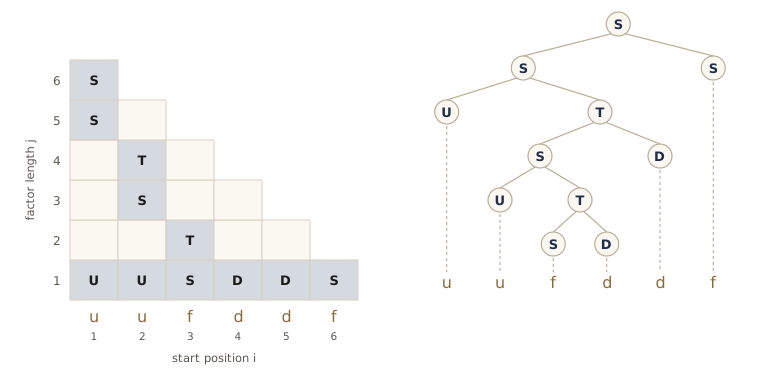
Two checks. First, the CNF grammar should generate exactly the ridges, which we can test against a direct definition (never below ground, ending at ground, not empty) on every string of length up to 7. Second, the random sentences of the original grammar should all parse. Then we classify strings with two grammars: ridges, and valleys (the same grammar with u and d exchanged).
def is_ridge(s):
    h = 0
    for ch in s:
        h += {"u": 1, "d": -1, "f": 0}[ch]
        if h < 0:
            return False
    return len(s) > 0 and h == 0

every = ["".join(p) for L in range(1, 8) for p in itertools.product("udf", repeat=L)]
agree = all(("S" in cyk(G_R_cnf, s)[0][0][len(s)]) == is_ridge(s) for s in every)
print(f"CYK membership equals the direct definition on all {len(every)} strings "
      f"up to length 7: {agree}")
sample = [generate(G_R, gen_g) for _ in range(200)]
print("all 200 random sentences of G_R parse:",
      all("S" in cyk(G_R_cnf, s)[0][0][len(s)] for s in sample))

swap = {"u": "d", "d": "u"}
G_V_cnf = {A: [tuple(swap.get(s, s) if len(r) == 1 else s for s in r) for r in rhss]
           for A, rhss in G_R_cnf.items()}
def grammar_class(s):
    return [name for name, G in (("ridge", G_R_cnf), ("valley", G_V_cnf))
            if "S" in cyk(G, s)[0][0][len(s)]] or ["neither"]
for s in ["uudfd", "ddffuu", "fff", "udduud"]:
    print(f"{s:7s} -> {grammar_class(s)}")
CYK membership equals the direct definition on all 3279 strings up to length 7: True
all 200 random sentences of G_R parse: True
uudfd   -> ['ridge']
ddffuu  -> ['valley']
fff     -> ['ridge', 'valley']
udduud  -> ['neither']
A flat string belongs to both languages, as it should, and a string that dips below ground and then climbs above it belongs to neither.
CYK’s cost is easy to read off the loops: \(O(n^2)\) table entries, each combining \(O(n)\) split points, so \(O(n^3)\) time for a fixed grammar (times the number of productions), and \(O(n^2)\) space. That is fine for short sentences and expensive for long ones.
Top-down parsing goes the other way: start from the root and choose productions, guided by the sentence, until the sentence is derived. A common strategy expands the leftmost variable and tries the productions that could produce the next unread character, backing up when a choice fails. Top-down parsers are often faster in practice but need care: with a left-recursive production such as \(S \to SS\), a naive top-down parser rewrites \(S\) as \(SS\) forever without reading a character, so such rules must first be rewritten away. Many practical parsers exploit a special structure of the grammar, finite-state machines for regular grammars being the simplest case.
Grammatical inference
So far the grammar was given. Can we learn it from example sentences? Grammatical inference differs from the statistical learning of earlier modules in an important way. A finite set of sentences is consistent with infinitely many grammars, among them the grammar that generates exactly those sentences and nothing else, and the grammar that generates every string. Positive examples alone cannot choose between these. Two devices make the problem tractable:
- Use negative examples too: a set \(\mathcal{D}^+\) of sentences known to be in the language and a set \(\mathcal{D}^-\) known not to be. With several categories, the positive examples of one category serve as negative examples for the others.
- Impose constraints and a simplicity bias: allow only the terminals seen in \(\mathcal{D}^+\), require every production to be used, restrict the type of grammar, and prefer the grammar with the fewest or shortest productions, Occam’s razor once more.
The general scheme starts from a minimal grammar and reads the positive examples one at a time. When a sentence cannot be parsed, it proposes new productions, simpler ones first, and accepts a proposal only if the sentence then parses and no negative example does. At the end, productions that no positive example needs are removed.
The cell implements this for regular grammars with a single variable \(S\), where every production has the form \(S \to w\) or \(S \to wS\) for a short terminal string \(w\). The target is the language of profiles made of flat steps and small bumps “ud”, with at least one flat step before each bump.
def parses(P, s):
    """Can S derive s with productions S -> w or S -> w S (w a terminal string)?"""
    for rhs in P:
        w = rhs.rstrip("S")
        if rhs.endswith("S"):
            if s.startswith(w) and len(s) > len(w) and parses(P, s[len(w):]):
                return True
        elif s == w:
            return True
    return False

def infer_grammar(D_pos, D_neg, alphabet="dfu", max_w=3):
    candidates = ["".join(p) + tail for L in range(1, max_w + 1)
                  for p in itertools.product(alphabet, repeat=L) for tail in ("", "S")]
    candidates.sort(key=len)                                   # simpler proposals first
    P = []
    for s in D_pos:
        if parses(P, s):
            print(f"  {s:10s} already parsed")
            continue
        for rhs in candidates:
            trial = P + [rhs]
            rejects_neg = not any(parses(trial, z) for z in D_neg)
            if rhs not in P and parses(trial, s) and rejects_neg:
                P.append(rhs)
                print(f"  {s:10s} add S -> {rhs}")
                break
    for rhs in list(P):                          # drop productions no example needs
        if all(parses([r for r in P if r != rhs], s) for s in D_pos):
            P.remove(rhs)
            print(f"  remove redundant S -> {rhs}")
    return P

D_pos = ["fud", "ffud", "fudfud", "ffudfudf", "fudf"]
D_neg = ["ud", "fu", "fdu", "udfud", "fudd", "fuud"]
P_learned = infer_grammar(D_pos, D_neg)
print("learned productions:", ["S -> " + r for r in P_learned])
for s in ["fffud", "fudffud", "ffff", "fudud", "uffd"]:
    print(f"   {s:8s} {'accepted' if parses(P_learned, s) else 'rejected'}")
  fud        add S -> fud
  ffud       add S -> fS
  fudfud     add S -> fudS
  ffudfudf   add S -> f
  fudf       already parsed
learned productions: ['S -> fud', 'S -> fS', 'S -> fudS', 'S -> f']
   fffud    accepted
   fudffud  accepted
   ffff     accepted
   fudud    rejected
   uffd     rejected
The learned grammar parses all the positive and none of the negative examples, uses only four short productions, and generalizes to longer strings such as “fffud”. It is not the only grammar consistent with the data, and it need not be the one we had in mind: every judgment it makes on new strings, such as accepting a string of flats alone, reflects the simplicity bias and the particular negative examples we happened to supply. More negative examples, or a different order of proposals, would change the answer. Practical grammatical inference relies on stronger constraints of this kind: for regular languages, learning can be phrased as adding states and transitions to a finite-state machine; for context-free languages there are specialized algorithms; and when a teacher can answer membership queries, learning becomes much faster.
Rule-based methods
When categories are best described by relationships among parts rather than by feature values, it is natural to write classifiers as if–then rules, for example
\[\text{IF } \mathrm{Round}(x) \text{ AND } \mathrm{HasStem}(x) \text{ AND } \mathrm{Red}(x) \text{ THEN } \mathrm{Cherry}(x).\]Rules are easy for people to read and check, and they fit data stored as relations in a database. Their weakness is the absence of any natural notion of probability, which makes them awkward when classes overlap heavily and the Bayes error is large. Rule systems are the core of expert systems in artificial intelligence but have had a more modest role in pattern recognition, so we keep this section short.
The building blocks are predicates, tests that return true or false, such as \(\mathrm{Red}(\cdot)\) or \(\mathrm{Adjacent}(\cdot, \cdot)\). The predicates can test numeric features, nominal attributes, strings, or relations between objects, and designing reliable detectors for them is usually much harder than learning the rules that combine them. Deciding \(\mathrm{Adjacent}(x, y)\) for two regions of a noisy camera image is a vision problem in its own right.
Rules come in two kinds.
- Propositional rules mention particular objects, constants, such as IF \(\mathrm{Round}(\mathit{Obj12})\) AND \(\mathrm{Red}(\mathit{Obj12})\) THEN \(\mathrm{Cherry}(\mathit{Obj12})\). Such a rule says nothing about \(\mathit{Obj13}\), however similar it is.
- First-order rules contain variables and so state general relations, for example IF \(\mathrm{Adjacent}(x, y)\) AND \(\mathrm{SameColor}(x, y)\) THEN \(\mathrm{SameRegion}(x, y)\), and IF \(\mathrm{SameRegion}(x, y)\) AND \(\mathrm{SameRegion}(y, z)\) THEN \(\mathrm{SameRegion}(x, z)\). The second rule is recursive, and it describes arbitrarily large regions with one line.
First-order rules can also contain functions, which return values, and terms built from them, such as IF \(\mathrm{Length}(x) > 2\,\mathrm{Width}(x)\) THEN \(\mathrm{Elongated}(x)\). This rule is exact and short. An axis-parallel tree on the features Length and Width could only approximate it with a staircase, as we saw for the diagonal problem, and would need more steps the more data it saw.
Classifying with a rule set is direct: evaluate the predicates on the new object and see which rules fire.
Learning rules
We have already met two ways to obtain rules: read them off a decision tree and prune them (C4.5), or infer a grammar. A third family learns rules directly by sequential covering: learn one rule that covers many positive examples and few negative ones, remove the positive examples it covers, and repeat until every positive example is covered. The result is a disjunction of conjunctive rules. Each single rule is grown greedily from general to specific: start with the rule that has no conditions (it covers everything), and repeatedly add the condition that makes it most accurate, until it covers no negative examples or no condition helps. For first-order rules, the candidate conditions include predicates with new variables, which is what systems for inductive logic programming search over; the propositional version below shows the covering loop on the houseplant data, with conditions of the form attribute = value and the Laplace-corrected accuracy \((p + 1)/(p + q + 2)\) of a rule that covers \(p\) positive and \(q\) negative examples as the score.
def learn_one_rule(samples, labels, target):
    conds, cov = [], list(range(len(samples)))
    score = lambda rows: (sum(labels[r] == target for r in rows) + 1) / (len(rows) + 2)
    while any(labels[r] != target for r in cov):
        options = [(score(sub), a, v, sub) for a in ATTRS if a not in dict(conds)
                   for v in ATTRS[a] for sub in [[r for r in cov if samples[r][a] == v]]
                   if any(labels[r] == target for r in sub)]
        if not options:
            break
        best = max(options, key=lambda o: o[0])
        if best[0] <= score(cov):
            break
        conds.append((best[1], best[2]))
        cov = best[3]
    return conds, cov

def sequential_covering(samples, labels, target):
    rules, remaining = [], list(range(len(samples)))
    while any(labels[r] == target for r in remaining):
        sub_s, sub_l = [samples[r] for r in remaining], [labels[r] for r in remaining]
        conds, cov = learn_one_rule(sub_s, sub_l, target)
        pos = [remaining[r] for r in cov if sub_l[r] == target]
        if not conds or not pos:
            break
        rules.append(conds)
        print(f"rule {len(rules)}: IF " + " AND ".join(f"{a}={v}" for a, v in conds)
              + f"   covers {len(pos)} positive, {len(cov) - len(pos)} negative")
        remaining = [r for r in remaining if r not in pos]
    return rules

learned = sequential_covering(plants, plant_labels, "thrives")
fires = lambda p: any(all(p[a] == v for a, v in conds) for conds in learned)
acc = np.mean([("thrives" if fires(p) else "struggles") == classify_nominal(plant_tree, p)
               for p in all_plants])
print(f"agreement with the true rule on all 36 plants: {acc:.3f}")
rule 1: IF water=weekly AND light=bright   covers 4 positive, 0 negative
rule 2: IF water=weekly AND light=medium   covers 3 positive, 0 negative
agreement with the true rule on all 36 plants: 0.944
The covering algorithm recovers the “weekly water and enough light” part of the true rule as two conjunctions, the same knowledge ID3 found, now stated directly as rules. Like ID3, it cannot discover the daily-humid-bright path, since no training plant shows it. The search is greedy, so the rule set need not be the most compact one; the usual final step is to simplify the disjunction with ordinary logic, here merging the two rules into (water = weekly AND light \(\neq\) low).
Summary
| Method | Data | How it is built | How it decides |
|---|---|---|---|
| CART | numeric or nominal attributes | greedy binary splits maximizing the impurity drop (Gini, entropy); grow fully, then cost-complexity pruning chosen by validation | follow one path; leaf majority or minimum-risk label; surrogate splits for missing values |
| Oblique (multivariate) tree | numeric features | a linear discriminant (e.g. LMS) at each node, threshold by impurity | one inner product per level |
| ID3 | nominal attributes (real values binned) | multiway splits, one branch per value, gain ratio; attributes not reused on a path | follow one path |
| C4.5 | mixed | thresholds for numeric, multiway for nominal, gain ratio; rule post-pruning | first matching rule, or weighted descent over branches for missing values |
| Naive / Boyer–Moore matching | strings | none (Boyer–Moore precomputes last-occurrence and good-suffix tables) | valid shifts; Boyer–Moore skips most of the text |
| Edit distance + nearest neighbor | strings | stored labeled prototypes | \(O(mn)\) dynamic program per comparison; label of the nearest string |
| Matching with errors / don’t-cares | strings | none | \(E[0, j] = 0\) dynamic program / correlations via the FFT |
| Grammar + CYK parser | strings with rule structure | grammar written by hand or inferred from \(\mathcal{D}^+, \mathcal{D}^-\) | membership in \(\mathcal{L}(G_i)\), \(O(n^3)\) for CNF |
| Sequential covering | attributes or relations | learn one greedy conjunction, remove covered positives, repeat | disjunction of if–then rules |
Ideas to carry forward:
- A tree is grown by repeatedly choosing the question with the largest drop in a strictly concave impurity. The choice among such impurities matters little; the choice of how large to let the tree grow matters a great deal, and growing fully then pruning with a validation set avoids the horizon effect of stopping rules.
- Trees are interpretable, handle nominal and mixed data, costs, and missing values gracefully, but they are unstable and can only cut parallel to the axes. The instability is what the resampling and combining methods of module 09 and Intro to ML, module 14 exploit.
- Without a metric we can still build one from operations: edit distance counts insertions, deletions, and substitutions, and dynamic programming computes it exactly. Nearest-neighbor classification then works on strings as it did on vectors.
- Grammars model strings produced by rules. The type of grammar sets both what can be expressed and what recognition costs, and learning a grammar needs negative examples and a bias toward simplicity, because finite data never pin one down.
Exercises
- Let \(i\) be a strictly concave function of the class-frequency vector. Show that for any binary split \(\Delta i \ge 0\), with equality exactly when both children have the same class frequencies as the parent. Then show that for entropy impurity \(\Delta i\) equals the mutual information between the category and the answer to the question, and conclude that a binary split can never reduce entropy impurity by more than one bit. What is the bound for a \(B\)-way split?
- With two categories, show that the variance impurity \(P(\omega_1)P(\omega_2)\) is the variance of a random variable equal to 1 for \(\omega_1\) and 0 for \(\omega_2\), and that the Gini impurity is the error rate of a classifier that labels each sample at the node by drawing a label at random from the node’s class frequencies. Then verify the twoing identity \(\Delta i = 2P_LP_R(q_L - q_R)^2\) step by step.
- Construct your own example, different from the one in the notes, of a parent node with three categories and a split for which the misclassification impurity does not decrease while the entropy does. Then find, with
grow, a data set on which a tree grown with misclassification impurity stops at the root although a two-level tree would classify perfectly. - Implement reduced-error pruning: working from the leaves upward, collapse any internal node whose collapse does not increase the validation error. Apply it to the fully grown tree of the box problem and compare the number of leaves and the test error with cost-complexity pruning. Why might the result be optimistic about its own accuracy?
- Show that the cost-weighted Gini impurity \(\sum_{i,j}\lambda_{ij}P(\omega_i)P(\omega_j)\) depends on \(\lambda_{ij}\) only through the symmetric part \((\lambda_{ij} + \lambda_{ji})/2\), and that for two categories it is a multiple of the Gini impurity. Then build a three-category example (counts and a cost matrix) for which the weighted Gini and the ordinary Gini prefer different splits, and check it with
impurity_drop. - Extend
best_splitso that training samples may have missing values (NaN): for each feature, compute the candidate drops using only the samples where that feature is present, as described in the notes. Test it on the correlated data of the missing-attributes subsection with 20% of the training values deleted at random. - CART also allows surrogate splits that go the other way (“is \(x_k \ge\) threshold?” sending samples left). Modify
surrogate_splitsto consider both directions, and construct data in which the best surrogate needs the reversed direction (for example \(x_2 = 1 - x_1\) plus noise). How much does the test error with \(x_1\) missing change? - Prove that the bad-character increment of Boyer–Moore never skips a valid shift. Then find a pattern and text over a two-letter alphabet for which the bad-character rule alone makes \(\Theta(nm)\) comparisons, and measure with
boyer_moore(..., use_good_suffix=False)and with the good-suffix rule switched on. - Add the interchange (transposition) of two adjacent characters as a fourth operation of cost 1 to
edit_table, derive the extra term of the recurrence, and verify your implementation against a version ofbfs_distancesthat also generates transpositions. - The ridge grammar is ambiguous: the string of \(k\) flat steps has many parse trees, because \(S \to SS\) can group the steps in different ways. Modify
cykto count parse trees instead of recording one, and show that the number of parses of \(\mathrm{f}^k\) is the Catalan number \(\frac{1}{k}\binom{2k-2}{k-1}\). Then write an unambiguous grammar for the same language. - Rerun
infer_grammarafter adding “ffff” to \(\mathcal{D}^-\), and then after changing the order in which the positive examples are read. Report the learned productions each time and explain the differences in terms of the simplicity bias. - In your own words: why does it make sense to call trees, string distances, and grammars “nonmetric” methods, and what does each of them use in place of a distance between feature vectors? Give one pattern recognition problem where you would reach for each.
Going further
- R. O. Duda, P. E. Hart, and D. G. Stork, Pattern Classification, 2nd ed., chapter 8. Problems 5–6 and 10 (impurity functions), 11 and 16 (costs and priors), 14–15 (missing attributes and the chi-squared test), 17 (gain ratio), 18–22 (string matching and Boyer–Moore), 26–29 (edit distance and don’t-care matching), 36–38 (Chomsky normal form and grammars), and 40 (grammatical inference) pair with the sections above. Computer exercises 1–5 build and prune trees, 6–8 cover string matching, 9–10 parsing, and 11 grammatical inference.
- L. Breiman, J. H. Friedman, R. A. Olshen, and C. J. Stone, Classification and Regression Trees (Wadsworth, 1984) — the CART book: impurity, twoing, surrogate splits, and cost-complexity pruning in full.
- J. R. Quinlan, “Induction of decision trees”, Machine Learning, 1986 — ID3 and the gain ratio; his book C4.5: Programs for Machine Learning (Morgan Kaufmann, 1993) describes C4.5 and its rule post-pruning.
- R. S. Boyer and J S. Moore, “A fast string searching algorithm”, Communications of the ACM, 1977; and R. A. Wagner and M. J. Fischer, “The string-to-string correction problem”, Journal of the ACM, 1974 — the original papers behind the two string algorithms of this module.
- J. E. Hopcroft, R. Motwani, and J. D. Ullman, Introduction to Automata Theory, Languages, and Computation — the Chomsky hierarchy, normal forms, the pumping lemmas, and CYK parsing with proofs.
- Related modules: nearest-neighbor rules in module 04, resampling, MDL, and combining classifiers in module 09, and trees as building blocks of committees and mixtures of experts in Intro to ML, module 14.
These notes follow the chapters of R. O. Duda, P. E. Hart, and D. G. Stork, Pattern Classification, 2nd edition (Wiley, 2001), the course text. The explanations, code, figures, and exercises here are written for this course; the book remains the reference, with the full derivations, worked examples, and many more problems.